data-driven traffic impact assessment tool for work … of education, research, and technology...

Data-Driven Traffic Impact Assessment Tool for Work ZonesFinal ReportMarch 2017

Sponsored bySmart Work Zone Deployment InitiativeFederal Highway Administration(TPF-5(295) and InTrans Project 15-535)Midwest Transportation CenterU.S. Department of Transportation Office of the Assistant Secretary for Research and Technology

About SWZDI Iowa, Kansas, Missouri, and Nebraska created the Midwest States Smart Work Zone Deployment Initiative (SWZDI) in 1999 and Wisconsin joined in 2001. Through this pooled-fund study, researchers investigate better ways of controlling traffic through work zones. Their goal is to improve the safety and efficiency of traffic operations and highway work.

About MTCThe Midwest Transportation Center (MTC) is a regional University Transportation Center (UTC) sponsored by the U.S. Department of Transportation Office of the Assistant Secretary for Research and Technology (USDOT/OST-R). The mission of the UTC program is to advance U.S. technology and expertise in the many disciplines comprising transportation through the mechanisms of education, research, and technology transfer at university-based centers of excellence. Iowa State University, through its Institute for Transportation (InTrans), is the MTC lead institution.

About InTransThe mission of the Institute for Transportation (InTrans) at Iowa State University is to develop and implement innovative methods, materials, and technologies for improving transportation efficiency, safety, reliability, and sustainability while improving the learning environment of students, faculty, and staff in transportation-related fields.

ISU Non-Discrimination Statement Iowa State University does not discriminate on the basis of race, color, age, ethnicity, religion, national origin, pregnancy, sexual orientation, gender identity, genetic information, sex, marital status, disability, or status as a U.S. veteran. Inquiries regarding non-discrimination policies may be directed to Office of Equal Opportunity, 3410 Beardshear Hall, 515 Morrill Road, Ames, Iowa 50011, Tel. 515-294-7612, Hotline: 515-294-1222, email [email protected].

NoticeThe contents of this report reflect the views of the authors, who are responsible for the facts and the accuracy of the information presented herein. The opinions, findings and conclusions expressed in this publication are those of the authors and not necessarily those of the sponsors.

This document is disseminated under the sponsorship of the U.S. DOT UTC program in the interest of information exchange. The U.S. Government assumes no liability for the use of the information contained in this document. This report does not constitute a standard, specification, or regulation.

The U.S. Government does not endorse products or manufacturers. If trademarks or manufacturers’ names appear in this report, it is only because they are considered essential to the objective of the document.

Quality Assurance StatementThe Federal Highway Administration (FHWA) provides high-quality information to serve Government, industry, and the public in a manner that promotes public understanding. Standards and policies are used to ensure and maximize the quality, objectivity, utility, and integrity of its information. The FHWA periodically reviews quality issues and adjusts its programs and processes to ensure continuous quality improvement.

Technical Report Documentation Page

1. Report No. 2. Government Accession No. 3. Recipient’s Catalog No.

4. Title 5. Report DateData-Driven Traffic Impact Assessment Tool for Work Zones March 2017

6. Performing Organization Code

7. Author(s) 8. Performing Organization Report No.Praveen Edara, Yohan Chang, Carlos Sun, and Henry Brown9. Performing Organization Name and Address 10. Work Unit No. (TRAIS)Department of Civil and Environmental Engineering University of Missouri-Columbia E2509 Lafferre Hall Columbia, MO 65211

11. Contract or Grant No.

Part of USDOT DTRT13-G-UTC3712. Sponsoring Organization Name and Address 13. Type of Report and Period CoveredSmart Work Zone Deployment Initiative Iowa Department of Transportation 800 Lincoln Way Ames, Iowa 50010 Midwest Transportation Center 2711 S. Loop Drive, Suite 4700 Ames, IA 50010-8664

Federal Highway Administration and Office of the Assistant Secretary for Research and Technology U.S. Department of Transportation 1200 New Jersey Avenue SE Washington, DC 20590

Final Report14. Sponsoring Agency CodePart of TPF-5(295) and Part of InTrans Project 15-535

15. Supplementary NotesVisit www.intrans.iastate.edu/smartwz/ for color pdfs of this and other Smart Work Zone Deployment Initiative research reports and www.intrans.iastate.edu for color pdfs of this and other research reports from InTrans. 16. AbstractTraditionally, traffic impacts of work zones have been assessed using planning software such as Quick Zone, custom spreadsheets, and others. These software programs generate delay, queuing, and other mobility measures but are difficult to validate due to the lack of field data necessary for validation. One alternative approach for assessing the travel time impacts of a work zone is through data mining. Historical data of travel times observed during work zones and normal conditions can be used for work zone planning and scheduling.

This project developed a prototype tool using historical data for work zones in the St. Louis region in Missouri. Data from 782 work zones on I-70, I-270, and MO 141 that occurred between January 2014 and October 2015 were used. Several data sources were utilized in this project. These included electronic alerts of work zone information such as start and end times, location, lane closure information, and travel times. Spatially, the data included the work zone segment, two upstream segments, and all segments within a 2-mile radius of the work zone. Two delay measures were used for quantifying impact of work zones on freeway segments: travel time delay based on historical average travel times for the segment and travel time delay based on historical 15th percentile travel time values.

A model was developed to estimate travel times for planned work zones at sites that may not have sufficient historical work zone data. The Random Forests technique was used to develop the model. Separate models were developed for interstate and arterial work zones using historical travel times and speed profiles, work zone and upstream segment lengths, lane closure information, and work zone schedule. The predicted travel times were then utilized to compute delays. A prototype of the data-driven traffic assessment tool was developed. The predicted travel times for both interstate and arterial work zones were within 5% error.

For demonstration purposes, the scope of the prototype was limited to two interstate corridors and one arterial corridor. The tool uses four types of input information: work zone location, roadway direction, work zone duration, and work zone type and lane closure information. The tool then uses this information to mine the historical data to identify any work zones that occurred at the same location in the past. If a match is found, the historical data is utilized to generate the expected delay measures. If a match is not found, the Random Forests prediction model is used to generate the expected delay measures.

17. Key Words 18. Distribution Statementhighway mobility models—historical data mining—Random Forests predictions—traffic assessment tool—travel time impacts—work-zone delays—work-zone planning

No restrictions.

19. Security Classification (of thisreport)

20. Security Classification (of thispage)

21. No. of Pages 22. Price

Unclassified. Unclassified. 56 NA Form DOT F 1700.7 (8-72) Reproduction of completed page authorized

DATA-DRIVEN TRAFFIC IMPACT ASSESSMENTTOOL FOR WORK ZONES

Final Report March 2017

Principal Investigator Praveen Edara, Associate Professor University of Missouri-Columbia

Co-Principal Investigators Carlos Sun, Associate Director

Henry Brown, Research Engineer Transportation Infrastructure Center, University of Missouri-Columbia

Research Assistant Yohan Chang

Authors Praveen Edara, Carlos Sun, Yohan Chang, and Henry Brown

Sponsored by Midwest Transportation Center, U.S. DOT Office of the Assistant Secretary for Research and Technology, and

FHWA Smart Work Zone Deployment Initiative Pooled Fund Study (TPF-5(295))

Preparation of this report was financed in part through funds provided by the Iowa Department of Transportation

through its Research Management Agreement with the Institute for Transportation

(InTrans Project 15-535)

A report from Institute for Transportation

Iowa State University 2711 South Loop Drive, Suite 4700

Ames, IA 50010-8664 Phone: 515-294-8103 / Fax: 515-294-0467

www.intrans.iastate.edu

v

TABLE OF CONTENTS

ACKNOWLEGMENTS ................................................................................................................ ix

EXECUTIVE SUMMARY ........................................................................................................... xi

INTRODUCTION ...........................................................................................................................1

DATA ACQUISITION AND ANALYSIS .....................................................................................3

1. Work Zone Information from Traffic Management Center Electronic Alerts ................3 2. Work Zone Duration, Length, and Lane Closure ............................................................4 3. Identifying Segments Affected by the Work Zone ..........................................................6 4. Travel Time Data .............................................................................................................7 5. Work Zone Travel Time Delay Measures .....................................................................10 6. Delays Computed Using Historical Data .......................................................................11 7. Delays on Adjacent Road Segments ..............................................................................15

TRAVEL DELAY PREDICTION MODEL .................................................................................17

1. Random Forests .............................................................................................................17 2. Building a Travel Time Prediction Model .....................................................................19

DEVELOPMENT OF PROTOTYPE TOOL ................................................................................25

1. Prototype Architecture ...................................................................................................25 2. System Requirements.....................................................................................................26 3. Installation......................................................................................................................26 4. Running the Prototype after Installation ........................................................................27 5. Prototype Features .........................................................................................................28 6. Output Features ..............................................................................................................29

CONCLUSIONS............................................................................................................................32

REFERENCES ..............................................................................................................................33

APPENDIX A: HISTOGRAMS OF TRAVEL TIME DELAYS .................................................35

APPENDIX B: STANDARD DEVIATIONS OF THE PREDICTION MODEL OUTPUT .......37

Less than One-Day Duration Work Zones.........................................................................37 More than One-Day Work Zones ......................................................................................38 Arterial Work Zones ..........................................................................................................39

vi

LIST OF FIGURES

Figure ES1. Work zone locations obtained from electronic alerts ............................................... xii Figure ES2. Framework of the travel time prediction model ...................................................... xiii Figure ES3. Screenshot for DDT_WZ software .......................................................................... xiv Figure ES4. Screenshot for output graphical user interface ........................................................ xiv Figure 1. Example of MoDOT’s electronic alert .............................................................................3 Figure 2. Work zone locations obtained from electronic alerts .......................................................4 Figure 3. Distribution of work zone durations .................................................................................5 Figure 4. Distribution of I-70 and I-270 work zones by lane closures ............................................5 Figure 5. Distribution of MO 141 work zones by lane closures ......................................................6 Figure 6. Comparison of work zone lengths ....................................................................................6 Figure 7. Work zone and upstream travel time segments ................................................................7 Figure 8. RITIS data query interface and detector deployment in St. Louis area ............................8 Figure 9. Mobility measures (top) and TMC codes (bottom) ..........................................................9 Figure 10. Data description of RITIS database ..............................................................................10 Figure 11. Histogram for HATT and reference TT for I-70 (less than one day) ...........................12 Figure 12. Histogram for HATT and reference TT for I-270 (less than one day) .........................13 Figure 13. Histogram for HATT and reference TT for I-70 (more than one day) .........................13 Figure 14. Histogram for HATT and reference TT for I-270 (more than one day) .......................14 Figure 15. Histograms for MO 141 travel times (less than one day) .............................................14 Figure 16. Histograms for MO 141 travel times (more than one day) ..........................................15 Figure 17. Identifying road segments within a certain radius of the work zone segment

(example of I-270 route) ...............................................................................................16 Figure 18. Overview of Random Forests .......................................................................................18 Figure 19. Overall framework of the travel time prediction model ...............................................19 Figure 20. Random Forests and Baseline predictions for less than one day work zones

(interstates) ....................................................................................................................21 Figure 21. Importance of variables in the prediction model for less than one day work

zones (interstates) ..........................................................................................................22 Figure 22. Random Forests and Baseline predictions for more than one day work zones

(interstates) ....................................................................................................................22 Figure 23. Importance of variables in the prediction model for more than one day work

zones (interstates) ..........................................................................................................23 Figure 24. Random Forests and Baseline predictions (arterial) .....................................................24 Figure 25. Importance of variables in the prediction model (arterial) ...........................................24 Figure 26. Architecture for the proposed prototype tool ...............................................................25 Figure 27. Folder for installing ......................................................................................................26 Figure 28. Screenshot of prototype installation .............................................................................27 Figure 29. Screenshot for 2_Run_after_Install folder ...................................................................27 Figure 30. Screenshot for DDT_WZ software ...............................................................................28 Figure 31. Screenshot for DDT_WZ graphical user interface .......................................................28 Figure 32. Screenshot for output graphical user interface .............................................................29 Figure 33. Successful initiation of the Random Forests prediction module ..................................30 Figure 34. Predicted travel times in R ...........................................................................................30 Figure 35. Spatial visualization of delays in Google Earth ...........................................................31

vii

Figure A1. One-mile HATT delay by each WZ event ID of the two interstates (less than one day duration for I-270 and I-70) .............................................................................35

Figure A2. Two-mile HATT delay by each WZ event ID of the two interstates (less than one day duration for I-270 and I-70) .............................................................................35

Figure A3. One-mile HATT delay by each WZ event ID of the two interstates (more than one day duration for I-270 and I-70) .............................................................................35

Figure A4. Two-mile HATT delay by each WZ event ID of the two interstates (more than one day duration for I-270 and I-70) .............................................................................36

Figure A5. One-mile HATT delay by each WZ event ID (MO 141 arterial) ................................36 Figure A6. Two-mile HATT delay by each WZ event ID (MO 141 arterial) ...............................36 Figure B1. Standard deviation and variance for SE results ...........................................................37 Figure B2. Standard deviation and variance for AE results ...........................................................38 Figure B3. Standard deviation and variance for SE results ...........................................................38 Figure B4. Standard deviation and variance for AE results ...........................................................39 Figure B5. Standard deviation and variance for SE results ...........................................................39 Figure B6. Standard deviation and variance for AE results ...........................................................40

LIST OF TABLES

Table 1. Studies pertaining to work zone traffic impact assessment ...............................................1 Table 2. AADT statistics for the study routes in 2015 ....................................................................4 Table 3. General statistics for work zone lengths ............................................................................6 Table 4. Travel time delay for the study corridors.........................................................................12 Table 5. Delays for segments within 1-mile and 2-mile radius of the work zones ........................16 Table 6. Variables used in the prediction model............................................................................20 Table 7. Results for travel time prediction (interstates) .................................................................21 Table 8. Results for travel time prediction (arterial) ......................................................................23 Table B1. Results for STDEV and variance for SE and AE results from TT prediction ..............37 Table B2. Results for STDEV and variance for SE and AE results from TT prediction ..............38 Table B3. Results for STDEV and variance for SE and AE results from TT prediction ..............39

ix

ACKNOWLEGMENTS

This project was funded by the Midwest Transportation Center, the U.S. Department of Transportation (DOT) Office of the Assistant Secretary for Research and Technology, and the Smart Work Zone Deployment Initiative (SWZDI) and Federal Highway Administration (FHWA) Pooled Fund Study TPF-5(295), involving the following state departments of transportation:

• Iowa (lead state) • Kansas • Missouri • Nebraska • Wisconsin

The authors would like to thank all of the sponsors for their financial support and technical assistance. The authors also express their gratitude to the following individuals who served on the technical advisory committee of the project: Dan Smith, Jon Nelson, and Jerica Holtsclaw of the Missouri DOT (MoDOT). Roozbeh Rahmani of the University of Missouri assisted with the analysis of MO 141 work zones.

xi

EXECUTIVE SUMMARY

Effective scheduling of roadwork requires accurate estimation of their traffic impacts. A variety of software tools have been developed to estimate work zone mobility impacts, including Quick Zone, custom spreadsheets, and QUEWZ. Microscopic simulation tools such as VISSIM and CORSIM have also been utilized.

These software tools generate mobility measures such as delay and queuing and can be used for scheduling work zones to minimize their impacts. Calibration and validation of these tools has been a challenge due to the lack of necessary field data. The underlying assumptions and the parameters of the queuing models do not allow for an accurate calibration for all performance measures such as queue length, delay, etc. In contrast to the previous approaches that used deterministic queuing methods (e.g., Quick Zone) to predict the traffic impacts of a planned work zone, this study developed a data-driven method that uses historical data to derive the performance measures. The proposed method helps to quantify the effect of a work zone by comparing performance measures such as speeds and travel times (or delay) with and without the presence of the work zone.

The proposed method was applied for a sample of work zones in the St. Louis region in Missouri. Gateway Guide, the Missouri Department of Transportation’s (MoDOT’s) traffic management center (TMC) in St. Louis, generates electronic alerts for various events, including work zones. These alerts provide real-time updates of the schedule, duration, and characteristics of work zones. The alert has several attributes of a work zone: current status (new, update, or cleared), type of work, route name, work zone location, and lane closure information. A procedure was then developed to automate the extraction of relevant work zone information from electronic alerts. The procedure involved first converting the alert into a text file and then splitting the message into the various work zone attributes described earlier. The location extracted from the alert was mapped onto Google Maps to identify the exact latitude and longitude. There were 801 work zone-related alerts (more than one alert for each work zone) from January 2014 to September 2015: 387 for I-70, 398 for I-270, and 16 for MO 141. Figure ES1 maps all the locations extracted from the electronic alerts.

xii

Map data ©2015 Google

Figure ES1. Work zone locations obtained from electronic alerts

The travel time data used in this project were obtained from the Regional Integrated Transportation Information System (RITIS). Queries were executed to obtain data for the work zone and two immediately upstream segments. Queried data from the RITIS database consist of several types: travel time and speed for segments and information on TMC codes identifying the segments. The impact of a specific freeway work zone in its vicinity was assessed using delay measures. Travel time delay was computed in several ways: using historical average travel time, using historical maximum travel time, and using historical 15th percentile travel time. The historical values include data for the same day of the week and time of day from previous three weeks.

In addition to the work zone and upstream segments, all adjacent road segments within a certain radius of the work zone are also analyzed to identify if the work zone had any impact on their travel times. Radius values of 1 mile and 2 miles from the work zone segment’s beginning location were examined. A prediction model was developed to predict travel times for planned work zones. The model development framework is shown in Figure ES2.

xiii

Figure ES2. Framework of the travel time prediction model

Data describing the work zone is inputted and used in conjunction with historical data. The Random Forests model then produces estimates of the future travel time delay (based on predicted travel times). A total of 27 variables are used in model development.

A prototype of the proposed data-driven traffic assessment tool was developed using the sample work zone data from the St. Louis region. Four types of input information are entered as input by a user: work zone coordinates, roadway direction, work zone duration, and lane closure information. The tool uses this information to mine the historical data to identify any work zones that occurred at the same location in the past. If a match is found, the data is utilized to generate the expected delay measures. If a match is not found, the travel time prediction model is used to generate the expected delay measures. The predicted travel times for both interstate and arterial work zones were within 5% error. A screenshot of the prototype’s input window is shown in Figure ES3.

xiv


Figure ES3. Screenshot for DDT_WZ software

A screenshot of the output window is shown in Figure ES4.


Figure ES4. Screenshot for output graphical user interface

The left side of the output window shows the work zone location on a map and the right side plots the travel time measures for a work zone segment. The table below the plot reports the delays (in minutes) for the work zone segment, upstream segments, and adjacent segments

xv

impacted by the work zone. On the left side of the output window, the red circle shows the 1-mile boundary around work zone and the yellow circle shows the 2-mile boundary. A summary of the input data entered by the user is printed at the bottom left of the screen.

The prototype can be enhanced in the future by including additional road segments from Smart Work Zone Deployment Initiative (SWZDI) pooled fund states. Other roadway types such as two-lane roads and minor arterials could also be added to the tool to help quantify the traffic impacts from work zones.

1

INTRODUCTION

State departments of transportation (DOTs) use several approaches to enhance safety and mobility in work zones. These approaches include better scheduling of work activity, improved traffic management plans, and use of innovative technology (e.g., queue warnings). Accurate assessment of traffic impacts are critical to work zone scheduling.

Research on the development of traffic impact assessment tools for work zones dates back to the late 1990s. State of the practice studies documenting these research efforts can be found in Edara (2006, 2009), Edara and Cottrell (2007), Edara et al. (2013), and Savolainen et al. (2015). Existing tools can be broadly categorized into four areas: impact assessment guidelines, traffic simulation applications, parametric approaches, and non-parametric approaches. Table 1 categorizes existing studies into these four areas.

Table 1. Studies pertaining to work zone traffic impact assessment

Emphasis area Literature Work zone impact assessment guidelines

Sankar et al. 2006, Ullman et al. 2011, Bourne et al. 2011, Mallela and Sadasivam 2011

Traffic simulation applications Chien et al. 2002, Meng and Weng 2010, Astarita et al. 2014, Edara 2006, Edara et al. 2013

Parametric approaches Jiang 2001, Schroeder and Rouphail 2010, Edara 2009, Edara et al. 2013, Dixon et al. 1996, Savolainen et al. 2015

Non-parametric approaches Ghosh-Dastidar and Adeli 2006, Weng and Meng 2012

A variety of software tools have been developed to estimate work zone mobility impacts, including Quick Zone, custom spreadsheets, and QUEWZ. Microscopic simulation tools such as VISSIM and CORSIM have also been utilized to quantify traffic impacts of work zones. These software tools generate mobility measures such as delay and queuing and can be used for scheduling work zones to minimize their impacts. However, calibration of these software tools and validation of their results has been a challenge, due to the lack of necessary field data (Edara et al. 2013). The underlying assumptions and parameters of the queuing models do not allow for an accurate calibration for all performance measures, such as queue length or delay.

In contrast to the previous approaches that used deterministic queuing methods (e.g., Quick Zone) to predict the traffic impacts of a planned work zone, this study developed a data-driven method that uses historical data to derive the performance measures. A statistical data mining approach uses historical data from work zones in a region to develop the relationships between the performance measures and the explanatory variables. The data-mining method helps to quantify the effect of work zones by comparing performance measures such as speeds, travel times (or delay), and queue length, with and without the presence of the work zone.

This data-driven approach relies on travel-time data continuously collected over the study

2

segments. Travel time data (e.g., probe-based) has recently become available over large coverage areas from third party sources such as the Regional Integrated Transportation Information System (RITIS), INRIX, and HERE. The quality of data obtained from these sources has been examined by Edwards and Fontaine (2012) for work zone applications and by Rakha et al. (2013) and Chen et al. (2015) for generic transportation applications.

A prototype of the data-driven approach was developed using historical data of work zones in the St. Louis region in Missouri. The prototype tool computes three travel time measures: 15th percentile travel time, historical average travel time, and historical maximum travel time. The historical values include data for the same day of the week and time of day from the previous three weeks. These measures are used to estimate work zone delays for both the work zone segment and all adjacent roadway segments within a radius of 1.0 mile and 2.0 miles around the work zone.

3

DATA ACQUISITION AND ANALYSIS

1. Work Zone Information from Traffic Management Center Electronic Alerts

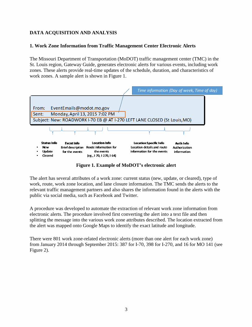
The Missouri Department of Transportation (MoDOT) traffic management center (TMC) in the St. Louis region, Gateway Guide, generates electronic alerts for various events, including work zones. These alerts provide real-time updates of the schedule, duration, and characteristics of work zones. A sample alert is shown in Figure 1.

Figure 1. Example of MoDOT’s electronic alert

The alert has several attributes of a work zone: current status (new, update, or cleared), type of work, route, work zone location, and lane closure information. The TMC sends the alerts to the relevant traffic management partners and also shares the information found in the alerts with the public via social media, such as Facebook and Twitter.

A procedure was developed to automate the extraction of relevant work zone information from electronic alerts. The procedure involved first converting the alert into a text file and then splitting the message into the various work zone attributes described. The location extracted from the alert was mapped onto Google Maps to identify the exact latitude and longitude.

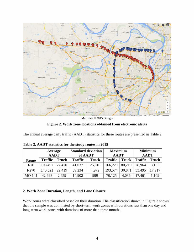
There were 801 work zone-related electronic alerts (more than one alert for each work zone) from January 2014 through September 2015: 387 for I-70, 398 for I-270, and 16 for MO 141 (see Figure 2).

4


Figure 2. Work zone locations obtained from electronic alerts

The annual average daily traffic (AADT) statistics for these routes are presented in Table 2.

Table 2. AADT statistics for the study routes in 2015

Route

Average AADT

Standard deviation of AADT

Maximum AADT

Minimum AADT

Traffic Truck Traffic Truck Traffic Truck Traffic Truck I-70 108,497 22,470 41,037 26,016 166,229 80,219 28,964 3,133 I-270 140,521 22,419 39,234 4,972 193,574 30,871 53,495 17,917

MO 141 42,698 2,459 14,902 999 70,125 4,036 17,461 1,109

2. Work Zone Duration, Length, and Lane Closure

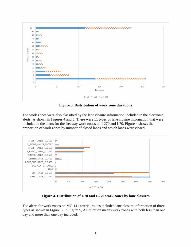
Work zones were classified based on their duration. The classification shown in Figure 3 shows that the sample was dominated by short-term work zones with durations less than one day and long-term work zones with durations of more than three months.

5

Figure 3. Distribution of work zone durations

The work zones were also classified by the lane closure information included in the electronic alerts, as shown in Figures 4 and 5. There were 11 types of lane closure information that were included in the alerts for the freeway work zones on I-270 and I-70. Figure 4 shows the proportion of work zones by number of closed lanes and which lanes were closed.

Figure 4. Distribution of I-70 and I-270 work zones by lane closures

The alerts for work zones on MO 141 arterial routes included lane closure information of three types as shown in Figure 5. In Figure 5, All duration means work zones with both less than one day and more than one day included.

0 50 100 150 200 250 300

0

1

5

10

15

20

25

30

35

40

50

60

70

80

90

90 +

Frequency

Wor

k Zo

ne d

ays

I-70 I-270 MO-141

0% 5% 10% 15% 20% 25% 30% 35% 40%

RIGHT_LANE_CLOSEDLEFT_LANE_CLOSED

STOPUSE_CENTER_LANES

RIGHT_SHOULDER_CLOSEDCENTER_LANE_CLOSED

CENTER_LANES_CLOSED2_RIGHT_LANES_CLOSED

2_LEFT_LANES_CLOSED3_RIGHT_LANES_CLOSED

3_LEFT_LANES_CLOSED

I270 I70

6

Figure 5. Distribution of MO 141 work zones by lane closures

Table 3 and Figure 6 show general statistics for less than one day and more than one day duration work zones.

Table 3. General statistics for work zone lengths

Length (miles)

Less than One Day More than One Day I-70 I-270 MO 141 I-70 I-270 MO 141

Mean 1.704 0.729 0.469 2.606 1.972 0.480 STDEV 4.231 0.381 0.389 5.240 1.812 0.313 Median 0.750 0.825 0.361 0.741 1.225 0.361

Figure 6. Comparison of work zone lengths

3. Identifying Segments Affected by the Work Zone

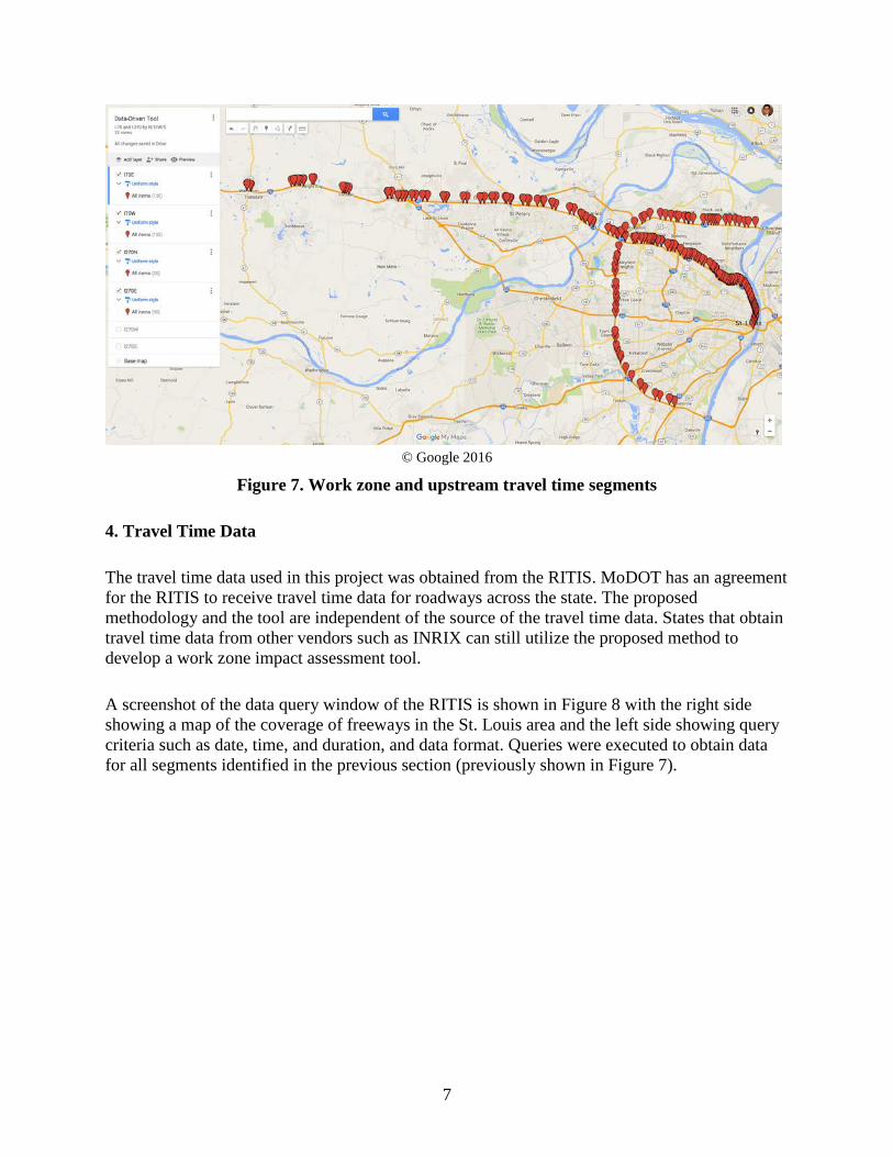
The electronic alerts contained information on the work zone locations. This information was used to determine three travel time segments: 1) the work zone segment, 2) the segment immediately upstream of work zone segment (1st upstream), and 3) the segment immediately upstream of the 1st upstream segment (2nd upstream). The identified upstream and work zone travel time segments for all work zones on I-70 and I-270 are shown in Figure 7.

0% 10% 20% 30% 40% 50% 60% 70% 80% 90%

LEFT_LANE_CLOSED

RIGHT_LANE_CLOSED

2_RIGHT_LANES_CLOSED

more-than one-day

less than one-day

All duration

0

1

2

3

4

5

6

I-70 I-270 MO-141 I-70 I-270 MO-141

Less than One-day More than One-days

Wor

k zo

ne L

engt

h (m

ile)

Mean STDEV Median

7

© Google 2016

Figure 7. Work zone and upstream travel time segments

4. Travel Time Data

The travel time data used in this project was obtained from the RITIS. MoDOT has an agreement for the RITIS to receive travel time data for roadways across the state. The proposed methodology and the tool are independent of the source of the travel time data. States that obtain travel time data from other vendors such as INRIX can still utilize the proposed method to develop a work zone impact assessment tool.

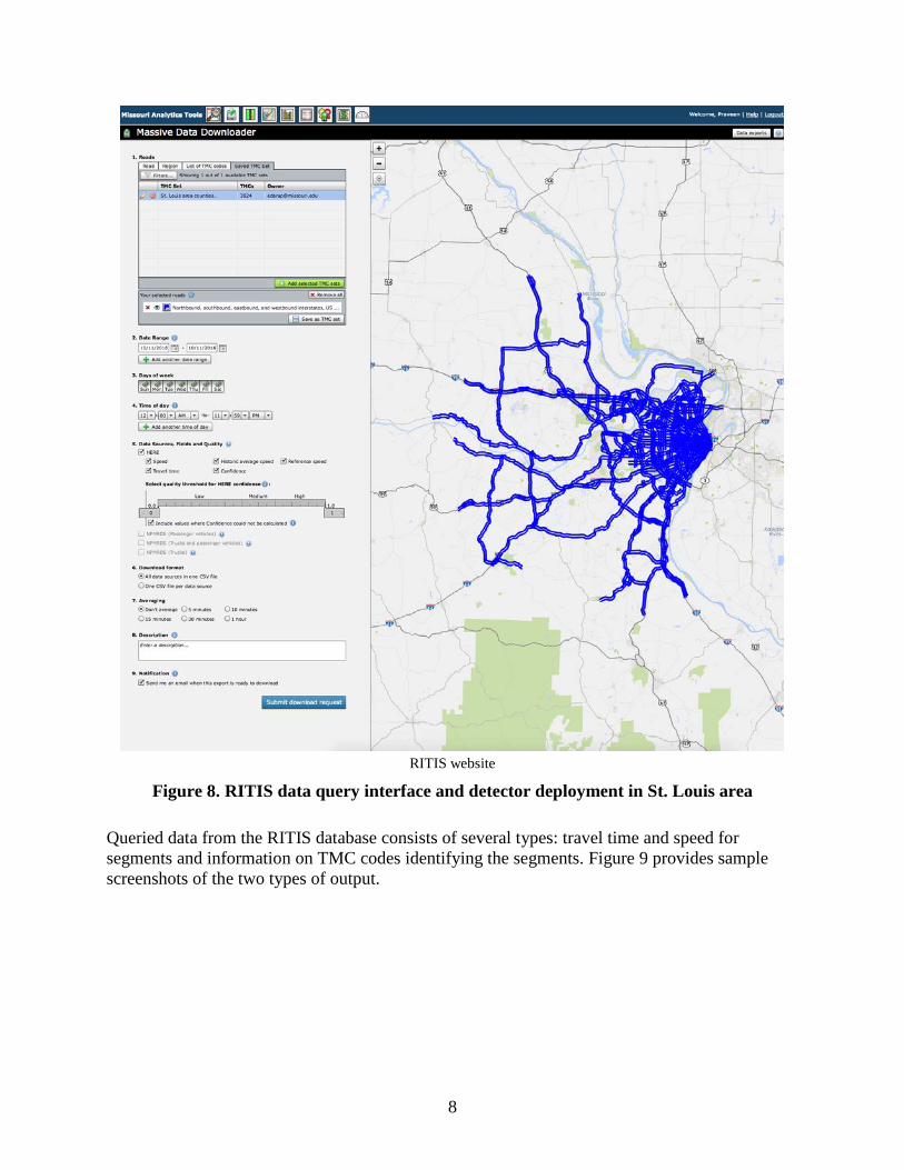
A screenshot of the data query window of the RITIS is shown in Figure 8 with the right side showing a map of the coverage of freeways in the St. Louis area and the left side showing query criteria such as date, time, and duration, and data format. Queries were executed to obtain data for all segments identified in the previous section (previously shown in Figure 7).

8

RITIS website

Figure 8. RITIS data query interface and detector deployment in St. Louis area

Queried data from the RITIS database consists of several types: travel time and speed for segments and information on TMC codes identifying the segments. Figure 9 provides sample screenshots of the two types of output.

9

Figure 9. Mobility measures (top) and TMC codes (bottom)

The travel time and speed information (top part of Figure 9) consists of seven fields: TMC code, time stamp, speed, average speed, reference speed, travel time, and confidence level. The bottom part of Figure 9 shows descriptive information of unique TMC codes that identify RITIS segments; this information includes road, direction, intersection, state, county, zip, start and end latitude/longitude, segment miles, and road order.

The time stamp includes information about time, i.e., date (month, day, and year) and time of day (hour, minute, and second). Three types of speeds (all in miles per hour) are reported for each segment in RITIS: prevailing speed, historical average speed, and reference speed (free flow speed). These speed measures, travel time, and confidence levels are defined in Figure 10.

10

RITIS data help

Figure 10. Data description of RITIS database

5. Work Zone Travel Time Delay Measures

The impact of a specific freeway work zone and its vicinity is assessed using delay measures. Three segments on freeways were analyzed for impact: work zone segment, 1st upstream segment, and 2nd upstream segment. While these segments capture the greatest impact of the work zone, other road segments adjacent to the freeway may also be impacted by the work zone. To this end, all adjacent road segments within a certain radius of the work zone were also analyzed to identify if the work zone had any impact on their travel times.

Freeway Segments

Two delay measures were adopted for quantifying the impact of work zones on freeway segments: travel time (TT) delay based on historical average travel times for the segment and TT delay based on historical 15th percentile travel time values.

Travel Time Delay Using Historical Average Travel Time

Travel time delay was calculated using the following equation:

�∑ �WZ TT𝑡𝑡 – HATT𝑡𝑡𝑆𝑆

�𝑇𝑇𝑡𝑡=1 � /𝑛𝑛𝑇𝑇 (1)

11

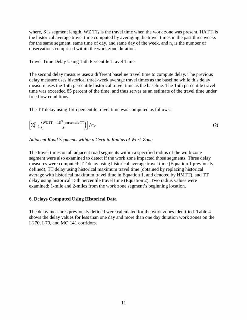
where, S is segment length, WZ TTt is the travel time when the work zone was present, HATTt is the historical average travel time computed by averaging the travel times in the past three weeks for the same segment, same time of day, and same day of the week, and nᵧ is the number of observations comprised within the work zone duration.

Travel Time Delay Using 15th Percentile Travel Time

The second delay measure uses a different baseline travel time to compute delay. The previous delay measure uses historical three-week average travel times as the baseline while this delay measure uses the 15th percentile historical travel time as the baseline. The 15th percentile travel time was exceeded 85 percent of the time, and thus serves as an estimate of the travel time under free flow conditions.

The TT delay using 15th percentile travel time was computed as follows:

�∑ �WZ TT𝑡𝑡 – 15𝑡𝑡ℎ percentile TT𝑆𝑆 �𝑇𝑇

𝑡𝑡=1 � /𝑛𝑛𝑇𝑇 (2)

Adjacent Road Segments within a Certain Radius of Work Zone

The travel times on all adjacent road segments within a specified radius of the work zone segment were also examined to detect if the work zone impacted those segments. Three delay measures were computed: TT delay using historical average travel time (Equation 1 previously defined), TT delay using historical maximum travel time (obtained by replacing historical average with historical maximum travel time in Equation 1, and denoted by HMTT), and TT delay using historical 15th percentile travel time (Equation 2). Two radius values were examined: 1-mile and 2-miles from the work zone segment’s beginning location.

6. Delays Computed Using Historical Data

The delay measures previously defined were calculated for the work zones identified. Table 4 shows the delay values for less than one day and more than one day duration work zones on the I-270, I-70, and MO 141 corridors.

12

Table 4. Travel time delay for the study corridors

Route Duration

Average TT delay using historical

average travel time (min/mile/WZ)

Average TT delay using 15th percentile

travel time (min/mile/WZ)

WZ 1UPS 2UPS WZ 1UPS 2UPS I-270 ≤ 1 day 0.72 0.15 0.03 0.54 0.19 0.03 I-70 ≤ 1 day 0.11 0.13 0.08 0.12 0.14 0.11

MO 141 ≤ 1 day 0.19 0.44 0.34 0.08 0.28 0.29 I-270 ≤ 1 day 0.15 0.15 0.91 0.25 0.26 0.22 I-70 ≤ 1 day 0.13 0.11 0.25 0.12 0.14 0.14

MO 141 ≤ 1 day 0.42 0.44 0.35 0.59 0.74 0.60

Delay values are reported using both historical average travel times (HATTs) and 15th percentile travel times. Table 4 shows that historical and 15th percentile delays differ in practice. Table 4 also shows that the delays across the three segments (WZ, 1UPS, 2UPS) do not have a set pattern.

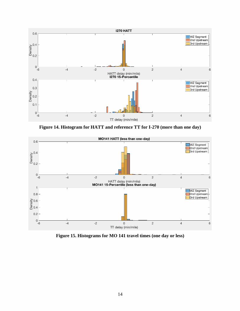
In addition to the average delays shown earlier in Table 3, histograms showing the delay distributions were also plotted as shown in Figures 11 through Figure 16.

Figure 11. Histogram for HATT and reference TT for I-70 (one day or less)

13

Figure 12. Histogram for HATT and reference TT for I-270 (one day or less)

Figure 13. Histogram for HATT and reference TT for I-70 (more than one day)

14

Figure 14. Histogram for HATT and reference TT for I-270 (more than one day)

Figure 15. Histograms for MO 141 travel times (one day or less)

15

Figure 16. Histograms for MO 141 travel times (more than one day)

7. Delays on Adjacent Road Segments

For every work zone included in the sample discussed earlier (2014 and 2015 work zones on I-270, I-70, and MO 141), all road segments (for which travel times were measured) within a 1-mile and 2-mile radius of the work zone were identified. The spherical law of cosines that computes distance between two points using their latitude and longitude, as shown in Equation 3, was adopted to accomplish this.

Spherical law of cosines

𝑑𝑑𝑑𝑑𝑑𝑑𝑡𝑡𝑑𝑑𝑛𝑛𝑑𝑑𝑑𝑑 = acos (𝑑𝑑𝑑𝑑𝑛𝑛𝜑𝜑1 × 𝑑𝑑𝑑𝑑𝑛𝑛𝜑𝜑2 + 𝑑𝑑𝑐𝑐𝑑𝑑𝜑𝜑1 × 𝑑𝑑𝑐𝑐𝑑𝑑𝜑𝜑2 × 𝑑𝑑𝑐𝑐𝑑𝑑∆𝜆𝜆) × 𝑅𝑅 (3)

Where, φ1 = latitude of work zone location φ2 = latitude of segment i Δλ = longitude of segment i - longitude of work zone location R = desired distance

Figure 17 shows an example involving a 2-mile radius around a work zone on I-270.

16


Figure 17. Identifying road segments within a certain radius of the work zone segment (example of I-270 route)

Table 5 shows the resulting delays using a 1-mile and 2-mile radii. One expected pattern was that delays were shorter for the 2-mile radius compared to the 1-mile radius, as congestion was farther away from the work zone.

Table 5. Delays for segments within 1-mile and 2-mile radius of the work zones Radius around

work zone segment Duration

Average TT delay with HATT

(min/mile/WZ)

Average TT delay with HMTT

(min/mile/WZ)

MAX TT delay with HATT

(min/mile/WZ)

MAX TT delay with HMTT

(min/mile/WZ) 1mile - all ≤ 1 day 0.10 0.11

0.63 0.64 2miles - all ≤ 1 day 0.09 0.10

1mile - I-270 ≤ 1 day 0.095 0.101 0.635 0.642 2miles - I-270 ≤ 1 day 0.080 0.084 0.249 0.265 1mile - I-70 ≤ 1 day 0.104 0.122 0.410 0.555 2miles - I-70 ≤ 1 day 0.097 0.109 0.322 0.374

1mile - all > 1 day 0.42 0.17 2.58 0.61

2miles - all > 1 day 0.21 0.16 1mile - I-270 > 1 day 0.378 0.220 0.988 0.403 2miles - I-270 > 1 day 0.188 0.205 0.371 0.327 1mile - I-70 > 1 day 0.462 0.109 2.584 0.612 2miles - I-70 > 1 day 0.226 0.102 2.584 0.229

1mile - all All 0.60 0.74 2.85 3.38

2miles - all All 0.22 0.27

17

TRAVEL DELAY PREDICTION MODEL

A travel time prediction model can be used to estimate travel times for planned work zones at sites that may not have sufficient historical work zone data. This chapter explains the procedure used to develop a travel time prediction model based on data from work zone sites on I-70, I-270, and MO 141 including travel times (up to 3 weeks), speed profiles (up to 3 weeks), work zone and upstream segment lengths, lane closure information, and work zone schedule. The predicted travel times were then utilized to compute delays.

1. Random Forests

The Random Forests statistical technique is commonly used for performing regression and classification (Breiman 2001). A single decision tree maps the input data (e.g., location, time, type of work zone) to a prediction, such as travel time. A forest refers to many decision trees that are developed and analyzed. By averaging the prediction from several trees instead of one tree, the problem of a single tree being sensitive to training set noise is mitigated.

In recent research conducted by Hou et al. (2015), Random Forests were shown to be a good technique to predict traffic conditions in work zones. Random Forests outperformed three other machine learning methods (multilayer feedforward neural networks, regression tree, and nonparametric regression) in predicting traffic flow and speed for planned work zone events. Consequently, this project employed the Random Forests technique to predict travel times for work zones. An introduction to regression trees and Random Forests can be found in Hou et al. (2015).

Figure 18 shows the general process of developing a Random Forests model and includes the following steps: initialization, sampling, tree growing, criteria checking, and ensemble generation (i.e., combining multiple trees).

18

Figure 18. Overview of Random Forests

The developed model can then be used for prediction. To predict a test data case, data are pushed down all the regression trees. Each tree produces a predicted traffic flow. The end result is the average of the predicted traffic flows of all trees. Random Forests constructs a measure of variable importance to help the user understand the mechanism of the prediction process and to eliminate less important variables (Hastie et al. 2009).

Some Random Forests parameters include the total number of predictors, p, the selected predictors, m, and the node size, i.e., tree complexity. Breiman (2001) recommends using m = p/3 and a minimum node size of five for regression applications.

19

2. Building a Travel Time Prediction Model

The model development framework is shown in Figure 19.

Figure 19. Overall framework of the travel time prediction model

Data describing the work zone is inputted and used in conjunction with historical data. The Random Forests model then produces estimates of the future travel time delay. A total of 27 variables were used in model development. Table 6 shows that these variables included general information, segment-specific information for three segments, and work zone characteristics. The input data were divided randomly into training (75%) and testing (25%) data, as is typical in modeling.

20

Table 6. Variables used in the prediction model

Categories Variable Name Descriptions

General Information

LOCATION Location ID at RITIS DATE Prediction date to be predicted StartTIME WZ start time to be predicted SegLen_UP2 Segment length for 2nd Upstream segment (mile) SegLen_UP1 Segment length for 1st Upstream segment (mile) SegLen_WZ Segment length where WZ presented (mile)

WZ Segment

TT_1WEEKAGO_WZ 1 week ago travel time at WZ segment location TT_2WEEKAGO_WZ 2 week ago travel time at WZ segment location TT_3WEEKAGO_WZ 3 week ago travel time at WZ segment location SPD_1WEEKAGO_WZ 1 week ago speed at WZ segment location SPD_2WEEKGO_WZ 2 week ago speed at WZ segment location SPD_3WEEKAGO_WZ 3 week ago speed at WZ segment location

1st Upstream from WZ Segment

TT_1WEEKAGO_2UP 1 week ago travel time at 1st Upstream location TT_2WEEKGO_2UP 2 week ago travel time at 1st Upstream location TT_3WEEKAGO_2UP 3 week ago travel time at 1st Upstream location SPD_1WEEKAGO_2UP 1 week ago speed at 1st Upstream location SPD_2WEEKGO_2UP 2 week ago speed at 1st Upstream location SPD_3WEEKAGO_2UP 3 week ago speed at 1st Upstream location

2nd Upstream from WZ Segment

TT_1WEEKAGO_3UP 1 week ago travel time at 2nd Upstream location TT_2WEEKGO_3UP 2 week ago travel time at 2nd Upstream location TT_3WEEKAGO_3UP 3 week ago travel time at 2nd Upstream location SPD_1WEEKAGO_3UP 1 week ago speed at 2nd Upstream location SPD_2WEEKGO_3UP 2 week ago speed at 2nd Upstream location SPD_3WEEKAGO_3UP 3 week ago speed at 2nd Upstream location

WZ Characteristics

Closed Lanes Closed lane type (i.e., right/left/center lane close) Total Number of lanes Total number of lanes for the segment Number of Closed Lanes Total number of closed lanes for the segment

For work zones on interstates, two Random Forests models were developed: one model for work zones with durations equal to or shorter than one day and one model for work zones with durations longer than one day. Two models were used instead of one because shorter duration work zones are fundamentally different than other work zones.

These models were developed using data from 253 work zones (≤1 day duration) and 513 work zones (>1 day duration) that occurred on I-70 and I-270 over a period of 22 months, from January 2014 through October 2015. The data were divided into training and testing sets as previously discussed. Random Forests models and baseline models were developed using these data.

The researchers developed two baseline models. The first baseline model used the average of

21

travel time at the same location and time in the prior three weeks (same as HATT previously discussed) as an estimate for the travel time with the work zone present. The second baseline model used travel time from one previous week instead of three weeks.

The prediction accuracies, root mean square error (RMSE), mean average error (MAE), and mean average percent error (MAPE), of the three models are shown in Table 7.

Table 7. Results for travel time prediction (interstates)

Travel Time prediction

(min) Duration Random Forests

Baseline (3 weeks average)

Baseline (1 week only)

WZS 1UPS 2UPS WZS 1UPS 2UPS WZS 1UPS 2UPS RMSE ≤ 1 day 0.23 0.17 0.08 0.45 0.33 0.11 0.46 0.25 0.13 MAE ≤ 1 day 0.06 0.05 0.02 0.11 0.08 0.04 0.12 0.07 0.04

MAPE ≤ 1 day 4.85% 4.56% 4.04% 7.41% 6.81% 6.29% 8.89% 9.24% 8.09% RMSE > 1 day 0.08 0.13 0.12 0.14 0.21 0.21 0.18 0.25 0.26 MAE > 1 day 0.02 0.03 0.04 0.04 0.06 0.06 0.05 0.06 0.07

MAPE > 1 day 3.95% 4.15% 4.18% 6.93% 6.97% 7.16% 7.97% 8.04% 8.31%

Across all measures and for both work zone and upstream segments, the Random Forests model outperformed the two baseline approaches. A graphical comparison is shown in Figure 20 for one day or less work zones and in Figure 22 for more than one day work zones. The importance of different variables in the prediction model are also plotted in Figures 21 and 23. The historical travel times (i.e., from one, two, and three weeks prior) exhibited the greatest impacts on the prediction accuracy.

Figure 20. Random Forests and baseline predictions for one day or less work zones

(interstates)

0%

1%

2%

3%

4%

5%

6%

7%

8%

9%

10%

WZS 1UPS 2UPS WZS 1UPS 2UPS WZS 1UPS 2UPS

RandomForests Baseline (3 weeks average) Baseline (1 week only)

MA

PE e

rror

22

Figure 21. Importance of variables in the prediction model for one day or less work zones

(interstates)

Figure 22. Random Forests and baseline predictions for more than one day work zones

(interstates)

0%

5%

10%

15%

20%

25%

30%

35%Im

port

ance

(%)

0%

1%

2%

3%

4%

5%

6%

7%

8%

9%



MA

PE e

rror

s

23

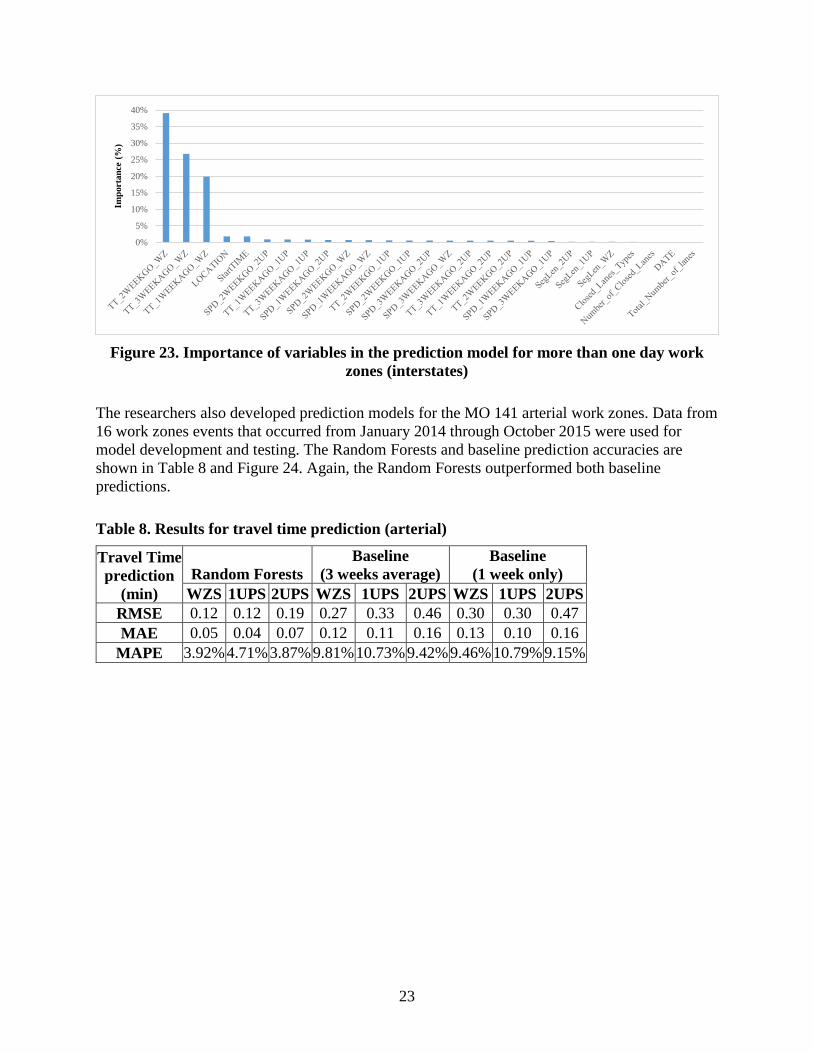
Figure 23. Importance of variables in the prediction model for more than one day work

zones (interstates)

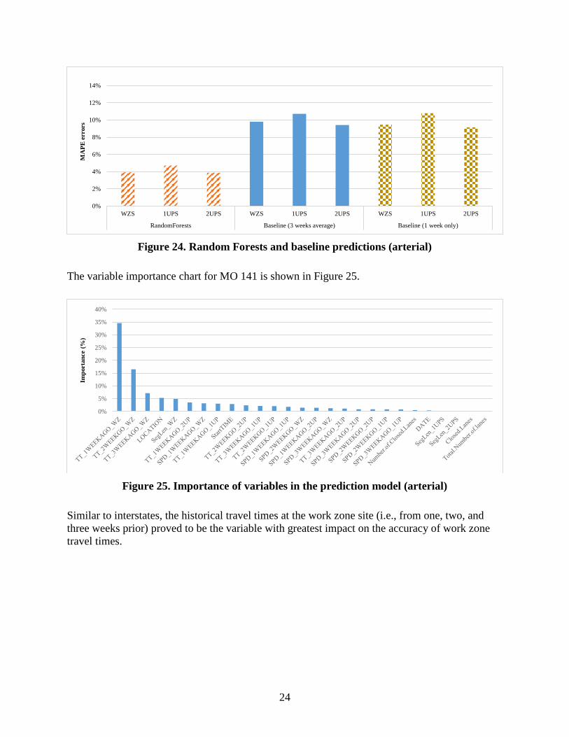
The researchers also developed prediction models for the MO 141 arterial work zones. Data from 16 work zones events that occurred from January 2014 through October 2015 were used for model development and testing. The Random Forests and baseline prediction accuracies are shown in Table 8 and Figure 24. Again, the Random Forests outperformed both baseline predictions.

Table 8. Results for travel time prediction (arterial)

Travel Time prediction

(min) Random Forests



WZS 1UPS 2UPS WZS 1UPS 2UPS WZS 1UPS 2UPS RMSE 0.12 0.12 0.19 0.27 0.33 0.46 0.30 0.30 0.47 MAE 0.05 0.04 0.07 0.12 0.11 0.16 0.13 0.10 0.16

MAPE 3.92% 4.71% 3.87% 9.81% 10.73% 9.42% 9.46% 10.79% 9.15%

0%

5%

10%

15%

20%

25%

30%

35%

40%Im

port

ance

(%)

24

Figure 24. Random Forests and baseline predictions (arterial)

The variable importance chart for MO 141 is shown in Figure 25.

Figure 25. Importance of variables in the prediction model (arterial)

Similar to interstates, the historical travel times at the work zone site (i.e., from one, two, and three weeks prior) proved to be the variable with greatest impact on the accuracy of work zone travel times.

0%

2%

4%

6%

8%

10%

12%

14%



MA

PE e

rror

s

0%

5%

10%

15%

20%

25%

30%

35%

40%

Impo

rtan

ce (%

)

25

DEVELOPMENT OF PROTOTYPE TOOL

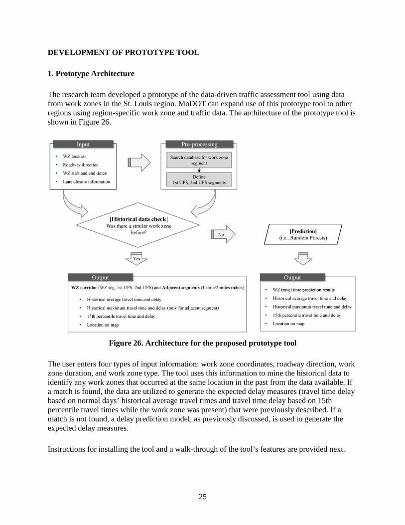
1. Prototype Architecture

The research team developed a prototype of the data-driven traffic assessment tool using data from work zones in the St. Louis region. MoDOT can expand use of this prototype tool to other regions using region-specific work zone and traffic data. The architecture of the prototype tool is shown in Figure 26.

Figure 26. Architecture for the proposed prototype tool

The user enters four types of input information: work zone coordinates, roadway direction, work zone duration, and work zone type. The tool uses this information to mine the historical data to identify any work zones that occurred at the same location in the past from the data available. If a match is found, the data are utilized to generate the expected delay measures (travel time delay based on normal days’ historical average travel times and travel time delay based on 15th percentile travel times while the work zone was present) that were previously described. If a match is not found, a delay prediction model, as previously discussed, is used to generate the expected delay measures.

Instructions for installing the tool and a walk-through of the tool’s features are provided next.

26

2. System Requirements

For best performance, the following minimum computational requirements are recommended for use of the prototype.

• RAM: 2 gigabytes or more • HDD empty space: 2.5 gigabyte or more • Recommended monitor resolution: 1,920 × 1,080 pixels per inch or higher • MATLAB Runtime (included in installation file) • Windows operating systems (Windows 7, 8, or 10) • Internet connection • Microsoft Excel • Google Earth (only to visualize delay plots spatially)

3. Installation

There are two folders: 1_Install and 2_Run_after_Install (see Figure 27).

Figure 27. Folder for installing

The first folder, 1_Install, is for installing the prototype tool and MATLAB Runtime environment

The installation file for this software tool, DDT_Install.exe file under 1_Install folder, and the MATLAB Runtime are installed together (see Figure 28).

27

Figure 28. Screenshot of prototype installation

4. Running the Prototype after Installation

Once the installation is complete, a user can run the prototype tool by double clicking the DDT_WZ.exe file located inside the 2_Run_after_Install folder, as shown in Figure 29.

Figure 29. Screenshot for 2_Run_after_Install folder

A screenshot of the tool after it’s launched is shown in Figure 30.

28


Figure 30. Screenshot for DDT_WZ software

5. Prototype Features

The user inputs coordinates, direction, duration, and type for a planned work zone as indicated by the callouts on the input window shown in Figure 31.


Figure 31. Screenshot for DDT_WZ graphical user interface

29

The location of the work zone is entered as latitude and longitude on the Coordinates tab. A dropdown menu was created from which a user can select the route and its direction. Work zone lane closure information and activity types can also be selected from drop-down menus.

6. Output Features

After entering all inputs, the user then clicks the OK button to run the tool. A screenshot of the output window is shown in Figure 32.


Figure 32. Screenshot for output graphical user interface

The left side of Figure 32 shows the work zone location on a map and the right side plots the travel time measures for the work zone segment. The table below the plot reports the delays (in minutes) for work zone segment, upstream segments, and adjacent segments impacted by the work zone. On the left side of the output window, the red circle shows the 1-mile boundary around work zone and the yellow circle shows the 2-mile boundary. A summary of the input data entered by the user is shown in a table at the bottom left of the screen.

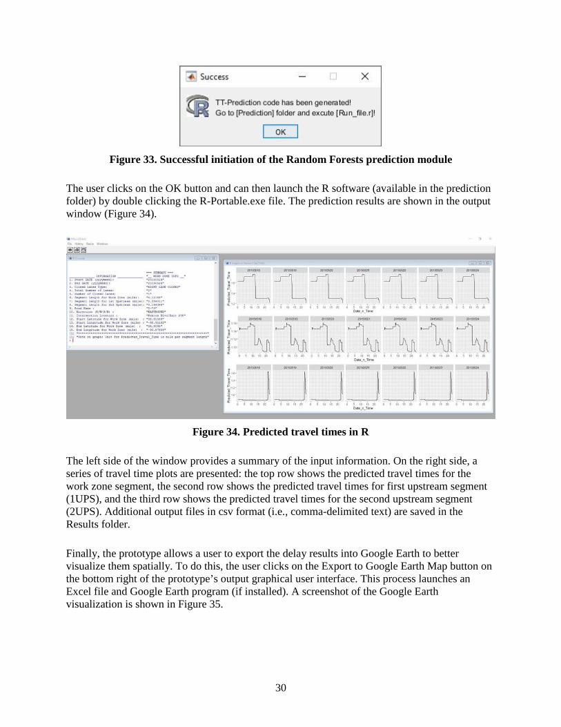
The Predict WZ-Travel Time button enables a user to predict the travel time for a planned work zone when there is no historical data for that location. The prediction is made using a trained Random Forests model discussed previously. Once a user clicks the Predict WZ-Travel Time button, the prototype runs additional scripts in the R program to predict travel times. The successful initiation window of the additional scripts in R is shown in Figure 33.

30

Figure 33. Successful initiation of the Random Forests prediction module

The user clicks on the OK button and can then launch the R software (available in the prediction folder) by double clicking the R-Portable.exe file. The prediction results are shown in the output window (Figure 34).

Figure 34. Predicted travel times in R

The left side of the window provides a summary of the input information. On the right side, a series of travel time plots are presented: the top row shows the predicted travel times for the work zone segment, the second row shows the predicted travel times for first upstream segment (1UPS), and the third row shows the predicted travel times for the second upstream segment (2UPS). Additional output files in csv format (i.e., comma-delimited text) are saved in the Results folder.

Finally, the prototype allows a user to export the delay results into Google Earth to better visualize them spatially. To do this, the user clicks on the Export to Google Earth Map button on the bottom right of the prototype’s output graphical user interface. This process launches an Excel file and Google Earth program (if installed). A screenshot of the Google Earth visualization is shown in Figure 35.

31

©2016 Google

Figure 35. Spatial visualization of delays in Google Earth

In Figure 35, three consecutive mainstream segments, work zone segment, 1st upstream, and 2nd upstream, are shown in different colors with work zone location outlined in red, 1st upstream outlined in yellow, and 2nd upstream outlined in orange. In addition, adjacent segments within 2 miles are outlined and highlighted in blue. The height of each polygon indicates the travel time delay for that segment; the taller the highlighted polygon, the greater the delay.

32

CONCLUSIONS

The researchers examined the feasibility of using historical data to develop a data-driven tool for assessing traffic impacts of work zones in this project. The research team used data from 766 freeway work zones (253 work zones with durations up to one day and 513 work zones with durations more than one day) and 16 arterial work zones over a period of 22 months, from January 2014 through October 2015.

A travel time prediction model, using Random Forests, was developed to estimate travel times for work zones at locations that may not have sufficient historical work zone data. The project culminated with the development of a prototype tool that incorporates historical data and prediction models for assessing traffic impacts at work zones.

The metropolitan St. Louis, Missouri region was used as the initial location for demonstrating the feasibility of the tool. When a planned work zone site has historical data available, the tool presents the historical data as the best estimate of the travel time. When historical data is not available for a location, the Random Forests prediction model produces estimates of the travel times.

The accuracies observed for both interstate and arterial work zones were acceptable, under 5% error in the predicted travel times. The scope of the prototype was limited to two interstate corridors and one arterial corridor.

The tool requires four types of input information: work zone location, roadway direction, work zone duration, and work zone type and lane closure information. The tool then makes predictions of travel times with and without work zone to compute the delays.

In the future, the tool can be enhanced in a few ways. First, additional routes from Smart Work Zone Deployment Initiative (SWZDI) states should be included. As shown in this project, travel time and work zone information are the key historical information required to add a corridor to use of the tool. The variability of this historical information among different SWZDI states also needs to be addressed. Second, while this study included work zones that occurred on an arterial, the sample size was smaller than the freeway work zones.

In the future, additional arterial work zones should be added to the tool. Similarly, work zones occurring on other types of roadways such as two lane roads and local roads should also be explored in future research.

33

REFERENCES

Astarita, V., V. P. Giofrè, G. Guido, and D. C. Festa. 2014. Traffic Delays Estimation in Two-Lane Highway Reconstruction. Procedia Computer Science, Vol. 32, pp. 331–338.

Bourne, J. S., C. Eng, G. L. Ullman, D. Gomez, B. Zimmerman, T. A. Scriba, R. D. Lipps, D. L. Markow, K. C. Matthews, D. L. Holstein, and R. Stargell. 2011. Scan 08-04: Best Practices in Work Zone Assessment, Data Collection, and Performance Evaluation. Arora and Associates, PC, Lawrenceville, NJ. onlinepubs.trb.org/onlinepubs/nchrp/docs/NCHRP20-68A_08-04.pdf.

Breiman, L. 2001. Random Forests. Machine Learning, Vol. 45, No. 1, pp. 5–32. Chen, M., X. Zhang, and E Green. 2015. Analysis of Historical Traffic Time Data. Kentucky

Transportation Center, University of Kentucky, Lexington, KY. www.ktc.uky.edu/files/2015/10/KTC_15_12_SPR12_444_1F.pdf.

Chien, S. I-J., D. G. Goulias, S. Yahalom, and S. M. Chowdhury. 2002. Simulation-Based Estimates of Delays at Freeway Work Zones. Journal of Advanced Transportation. Vol. 36, No. 2, pp. 131–156.

Dixon, K. K., J. E. Hummer, and A. R. Lorscheider. 1996. Capacity for North Carolina Freeway Work Zones. Transportation Research Record: Journal of the Transportation Research Board, No. 1529, pp. 27–34.

Edara, P. 2006. Estimation of Traffic Impacts at Work Zones: State of the Practice. Virginia Transportation Research Council, Charlottesville, VA. www.virginiadot.org/vtrc/main/online%5Freports/pdf/06-r25.pdf.

Edara, P. 2009. Evaluation of Work Zone Enhancement Software. Missouri Department of Transportation, Jefferson City, MO. library.modot.mo.gov/RDT/reports/Ri07062/or10006.pdf.

Edara, P. and B. H. J. Cottrell, Jr. 2007. Estimation of Traffic Mobility Impacts at Work Zones: State of the Practice. 86th Annual Meeting of the Transportation Research Board, January 21–25, 2007, Washington, DC. www.workzonesafety.org/files/documents/database_documents/07-0255.pdf.

Edara, P., C. Sun, and Z. Zhu. 2013. Calibration of Work Zone Impact Analysis Software for Missouri. Missouri Department of Transportation, Jefferson City, MO, and Mid-America Transportation Center, University of Nebraska-Lincoln, NE. library.modot.mo.gov/RDT/reports/TRyy1306/cmr14-004.pdf.

Edwards, M. B. and M. D. Fontaine. 2012. Investigation of Travel Time Reliability in Work Zones with Private-Sector Data. Transportation Research Record: Journal of the Transportation Research Board, No. 2272, pp. 9–18.

Ghosh-Dastidar, S. and H. Adeli. 2006. Neural Network-Wavelet Microsimulation Model for Delay and Queue Length Estimation at Freeway Work Zones. Journal of Transportation Engineering, Vol. 132, No. 4, pp. 331–341.

Hastie, T., R. Tibshirani, and J. Friedman. 2009. The Element of Statistical Learning: Data Mining, Inference, and Prediction. Second Edition. Springer-Verlag New York, NY.

Hou, Y., P. Edara, and C. Sun. 2015. Traffic flow forecasting for urban work zones, IEEE Transactions on Intelligent Transportation Systems, Vol. 16, No. 4, pp. 1761–1771.

Jiang, Y. Estimation of Traffic Delays and Vehicle Queues at Freeway Work Zones. 2001. 80th Annual Meeting of the Transportation Research Board, January 7–11, 2001, Washington, DC. www.workzonesafety.org/files/documents/database_documents/00346.pdf.

34

Mallela J. and S. Sadasivam, 2011. Work Zone Road User Costs: Concepts and Applications. Federal Highway Administration, Office of Operations, Washington, DC. ops.fhwa.dot.gov/wz/resources/publications/fhwahop12005/fhwahop12005.pdf.

Meng, Q. and J. Weng. 2010. Cellular Automata Model for Work Zone Traffic. Transportation Research Record: Journal of the Transportation Research Board, No. 2188, pp. 131–139.

Rakha, H., H. Chen, A. Haghani, and K. F. Sadabadi. 2013. Assessment of Data Quality Needs for Use in Transportation Applications. Mid-Atlantic Universities Transportation Center, Larson Transportation Institute, Pennsylvania State University, University Park, PA.

Sankar P., K. Jeannotte, J. P. Arch, M. Romero, and J. E. Bryden. 2006. Work Zone Impacts Assessment: An Approach to Assess and Manage Work Zone Safety and Mobility Impacts of Road Projects. Federal Highway Administration, Office of Transportation Operations, Washington, DC. ops.fhwa.dot.gov/wz/resources/final_rule/wzi_guide/wzi_guide.pdf.

Savolainen, P. T., T. J. Gates, T. Barrette, E. Rista, T. K. Datta, and S. E. Ranft. 2015. Balancing the Costs of Mobility Investments in Work Zones – Phase 1 Final Report. Michigan Department of Transportation, Lansing, MI. www.michigan.gov/documents/mdot/RC1630_491364_7.pdf.

Schroeder, B. J. and N. M. Rouphail. 2010. Estimating Operational Impacts of Freeway Work Zones on Extended Facilities. Transportation Research Record: Journal of the Transportation Research Board, No. 2169, pp. 70–80.

Ullman G. L., T. J. Lomax, and T Scriba. 2011. A Primer on Work Zone Safety and Mobility Performance Measurement. Federal Highway Administration, Office of Operations, Washington, DC. ops.fhwa.dot.gov/wz/resources/publications/fhwahop11033/fhwahop11033.pdf.

Weng, J. and Q. Meng. 2012. Ensemble Tree Approach to Estimating Work Zone Capacity. Transportation Research Record: Journal of the Transportation Research Board, No. 2286, pp. 56–67.

35

APPENDIX A: HISTOGRAMS OF TRAVEL TIME DELAYS

Figure A1. One-mile HATT delay by each WZ event ID of the two interstates (one day or

less duration for I-270 and I-70)

Figure A2. Two-mile HATT delay by each WZ event ID of the two interstates (one day or

less duration for I-270 and I-70)

Figure A3. One-mile HATT delay by each WZ event ID of the two interstates (more than

one day duration for I-270 and I-70)

-

0.1

0.2

0.3

0.4

0.5

0.61 6 11 16 21 26 31 36 41 46 51 56 61 66 71 76 81 86 91 96 101

106

111

116

121

126

131

136

141

146

151

156

161

166

171

176

181

186

191

196

201

206

211

216

221

226

231

236

241

246

251

TT d

elay

(min

/mile

)

WZ Event ID

-

0.1

0.2

0.3

0.4

0.5

0.6

1 6 11 16 21 26 31 36 41 46 51 56 61 66 71 76 81 86 91 96 101

106

111

116

121

126

131

136

141

146

151

156

161

166

171

176

181

186

191

196

201

206

211

216

221

226

231

236

241

246

251

TT d

elay

(min

/mile

)

WZ Event ID

-

0.5

1.0

1.5

2.0

2.5

3.0

1 11 21 31 41 51 61 71 81 91 101

111

121

131

141

151

161

171

181

191

201

211

221

231

241

251

261

271

281

291

301

311

321

331

341

351

361

371

381

391

401

411

421

431

441

451

461

471

481

491

501

511

TT d

elay

(min

/mile

)

WZ Event ID

36

Figure A4. Two-mile HATT delay by each WZ event ID of the two interstates (more than

one day duration for I-270 and I-70)

Figure A5. One-mile HATT delay by each WZ event ID (MO 141 arterial)

Figure A6. Two-mile HATT delay by each WZ event ID (MO 141 arterial)

-

0.1

0.1

0.2

0.2

0.3

0.3

0.4

0.4

1 11 21 31 41 51 61 71 81 91 101

111

121

131

141

151

161

171

181

191

201

211

221

231

241

251

261

271

281

291

301

311

321

331

341

351

361

371

381

391

401

411

421

431

441

451

461

471

481

491

501

511

TT d

elay

(min

/mile

)

WZ Event ID

0.0

0.1

0.2

0.3

0.4

0.5

0.6

0.7

1458 1366 1184 1703 665 1032 283 1533 967 1605 578 954 155 1540 1357 1937

TT D

elay

(min

/mile

)

WZ Event ID

0.0

0.1

0.2

0.3

0.4

0.5

0.6

0.7

1458 1366 1184 1703 665 1032 283 1533 967 1605 578 954 155 1540 1357 1937

TT D

elay

(min

/mile

)

WZ Event ID

37

APPENDIX B: STANDARD DEVIATIONS OF THE PREDICTION MODEL OUTPUT

Standard deviation (STDEV) and variance for squared errors (SE) and absolute errors (AE) are shown in Table B1, Figure B1, and Figure B2 for each predictor and each segment.

One Day or Less Duration Work Zones

Table B1. Results for STDEV and variance for SE and AE results from TT prediction

Random Forests



WZS 1UPS 2UPS WZS 1UPS 2UPS WZS 1UPS 2UPS STDEV for SE 0.665 0.730 0.192 1.979 1.992 0.216 2.013 0.764 0.240

Variance for SE 0.442 0.533 0.037 3.915 3.967 0.047 4.051 0.583 0.057 STDEV for AE 0.228 0.201 0.084 0.465 0.337 0.108 0.470 0.223 0.121

Variance for AE 0.052 0.040 0.007 0.216 0.114 0.012 0.221 0.050 0.015

Figure B1. Standard deviation and variance for SE results

0.0

0.5

1.0

1.5

2.0

2.5

3.0

3.5

4.0

4.5



STDEV for SE

Variance for SE

38

Figure B2. Standard deviation and variance for AE results

More than One Day Duration Work Zones


Random Forests





Variance for AE 0.006 0.016 0.014 0.019 0.040 0.042 0.031 0.060 0.0633


0.0

0.1

0.2

0.3

0.4

0.5

0.6

0.7

0.8

0.9

1.0



0

1

2

3

4

5

6



STDEV for SE Variance for SE

39


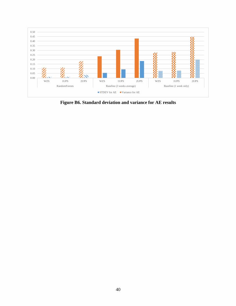
Arterial Work Zones


Random Forests





Variance for AE 0.013 0.013 0.034 0.056 0.094 0.184 0.076 0.080 0.200


0.0

0.1

0.1

0.2

0.2

0.3

0.3



STDEV for AE Variance for AE

0.0

0.5

1.0

1.5

2.0

2.5

3.0



STDEV for SE Variance for SE

40


0.00

0.05

0.10

0.15

0.20

0.25

0.30

0.35

0.40

0.45

0.50



STDEV for AE Variance for AE

data-driven traffic impact assessment tool for work … of education, research, and technology...

Documents