data driven rna structure determination - school of informatics
TRANSCRIPT
Data Driven RNA Structure
Determination
Wolfgang Lehrach
Master of Science
School of Informatics
University of Edinburgh
2003
(Graduation date: December 2003)

Abstract
This project presents a novel unsupervised learning approach to learning to de-
termine the structure of RNA molecules with little prior explicit knowledge of
RNA and only a database of sequences and their structures. The approach is
based upon adapting the parameters to maximise the probability of the correct
real life structure given the sequence. This was done with the aim of generalising
to novel sequences. A simple form of motif recognition is incorporated to improve
the ability to use the data within the database.
Rosetta style MCMC simulated annealing and conjugate gradient descent are
implemented to determine the structure with the highest probability given a
sequence and energy function.
Overall it was found that while the novel learning algorithm performed very
well, performance was limited by the choice of a simplest energy function with
few parameters which could only express how to fold molecules of low complexity
and which had to approximate more complex molecules.
i

Declaration
I declare that this thesis was composed by myself, that the work contained herein
is my own except where explicitly stated otherwise in the text, and that this work
has not been submitted for any other degree or professional qualification except
as specified.
(Wolfgang Lehrach)
ii

Table of Contents
1 Introduction 2
1.1 Overview . . . . . . . . . . . . . . . . . . . . . . . . . . . . . . . . 2
1.2 What is RNA and Why Determine its Structure . . . . . . . . . . 3
1.2.1 What RNA is made of . . . . . . . . . . . . . . . . . . . . 3
1.2.2 What is DNA . . . . . . . . . . . . . . . . . . . . . . . . . 7
1.2.3 What are Proteins . . . . . . . . . . . . . . . . . . . . . . 7
1.2.4 Different levels of structure . . . . . . . . . . . . . . . . . . 8
1.3 Mathematical Background . . . . . . . . . . . . . . . . . . . . . . 8
1.3.1 Probability and Sampling theory . . . . . . . . . . . . . . 8
1.3.2 The Metropolis Method . . . . . . . . . . . . . . . . . . . 10
1.4 Other approaches considered . . . . . . . . . . . . . . . . . . . . . 11
1.5 Temporal issues . . . . . . . . . . . . . . . . . . . . . . . . . . . . 11
1.6 Synopsis of the Rest of the Dissertation . . . . . . . . . . . . . . . 11
2 Literature review 13
2.1 Problem Feasibility of Structure Determination of RNA and Proteins 13
2.2 MFold . . . . . . . . . . . . . . . . . . . . . . . . . . . . . . . . . 14
2.2.1 Relative advantages and disadvantages . . . . . . . . . . . 14
2.3 Rosetta . . . . . . . . . . . . . . . . . . . . . . . . . . . . . . . . 17
2.3.1 Scoring function . . . . . . . . . . . . . . . . . . . . . . . . 17
2.3.2 Sampling of the Protein Space . . . . . . . . . . . . . . . . 19
2.3.3 Result processing . . . . . . . . . . . . . . . . . . . . . . . 19
2.3.4 Relative Advantages and Disadvantages . . . . . . . . . . . 20
iii

3 Methodology 21
3.1 Techniques used . . . . . . . . . . . . . . . . . . . . . . . . . . . . 21
3.1.1 Why use Probability Theory . . . . . . . . . . . . . . . . . 21
3.1.2 Defining P (C | Ψ, seq) . . . . . . . . . . . . . . . . . . . . 21
3.1.3 Increasing the Probability of a Structure for a Given Sequence 22
3.1.4 Finding the Structure given the Sequence of an RNAMolecule 24
3.1.5 Rossetta-style Simulated Annealing to find all Minima . . 25
3.2 Modelling the Structure of the RNA Molecule . . . . . . . . . . . 25
3.2.1 Why use a High Level Molecule Representation . . . . . . 25
3.2.2 Cartesian ’xyz’ Molecule Representation . . . . . . . . . . 26
3.2.3 Chain Spherical ’rtp’ Molecule Representation . . . . . . . 27
3.2.4 Bond and Torsion angle based . . . . . . . . . . . . . . . . 28
3.2.5 Data preprocessing . . . . . . . . . . . . . . . . . . . . . . 29
3.3 Defining the Energy function . . . . . . . . . . . . . . . . . . . . . 30
3.3.1 Requirements . . . . . . . . . . . . . . . . . . . . . . . . . 30
3.3.2 Scoring the bonds between neighbours . . . . . . . . . . . 30
3.3.3 Incorporating Base to Base interactions . . . . . . . . . . . 32
3.3.4 Initial Parameter Settings . . . . . . . . . . . . . . . . . . 34
3.4 Incorporating common motif recognition . . . . . . . . . . . . . . 34
3.4.1 Choosing motifs . . . . . . . . . . . . . . . . . . . . . . . . 34
3.4.2 Comparing structures . . . . . . . . . . . . . . . . . . . . . 35
3.5 Implementation Issues . . . . . . . . . . . . . . . . . . . . . . . . 36
3.5.1 Development Environment and Language . . . . . . . . . . 36
3.5.2 Regression checking . . . . . . . . . . . . . . . . . . . . . . 37
3.5.3 Vectorization, Optimisation and Benchmarking . . . . . . 37
3.5.4 Parallelizing the code . . . . . . . . . . . . . . . . . . . . . 37
3.6 Evaluating the Learning of the Parameters Ψ . . . . . . . . . . . . 38
3.6.1 Initial Teething Problems . . . . . . . . . . . . . . . . . . 38
3.6.2 Learning an Artifical Hairpin Structure . . . . . . . . . . . 39
3.6.3 Random folding . . . . . . . . . . . . . . . . . . . . . . . . 39
3.6.4 Real data . . . . . . . . . . . . . . . . . . . . . . . . . . . 40
iv

4 Results 41
4.1 Effects of Different Structural Repressentions on Structure Deter-
mination . . . . . . . . . . . . . . . . . . . . . . . . . . . . . . . . 41
4.2 Hairpin results . . . . . . . . . . . . . . . . . . . . . . . . . . . . 41
4.2.1 Adapting the Initial Parameter Settings . . . . . . . . . . 41
4.2.2 Adapting Difficult Parameter Settings . . . . . . . . . . . 43
4.3 Rederiving the Parameters of Random Folded Data . . . . . . . . 47
4.4 Real RNA data results . . . . . . . . . . . . . . . . . . . . . . . . 47
5 Conclusion 49
5.1 Concluding Remarks and Observations . . . . . . . . . . . . . . . 49
5.2 Unsolved Problems . . . . . . . . . . . . . . . . . . . . . . . . . . 50
5.3 Suggestions For Further Work . . . . . . . . . . . . . . . . . . . . 51
5.3.1 Integrating Temporal Information . . . . . . . . . . . . . . 51
5.3.2 Expanding upon Motif Recognition . . . . . . . . . . . . . 51
5.3.3 Improving the energy function: . . . . . . . . . . . . . . . 51
5.3.4 Implementation in a Different Language . . . . . . . . . . 52
5.3.5 A Fully Cross Validated Run . . . . . . . . . . . . . . . . . 52
A Structure produced by Real RNA Molecules without Motifs 53
B Structure produced by Real RNA Molecules with Motifs 58
Bibliography 62
v

List of Figures
1.1 Structural determination given an RNA sequence . . . . . . . . . 2
1.2 Chemical structure of DNA . . . . . . . . . . . . . . . . . . . . . 4
1.3 Central dogma of biology - should I include this? should I cite it
from CBD notes? . . . . . . . . . . . . . . . . . . . . . . . . . . . 5
2.1 Buried vs non-buried Penv terms in Rosetta . . . . . . . . . . . . . 18
3.1 Chain Spherical co-ordinate system . . . . . . . . . . . . . . . . . 28
3.2 Updates required in Cartesian Representation vs Chain Spherical 29
3.3 Expressing bond preferences of sequential bases in terms of distance 31
3.4 Artificial hairpin based on loop of Transfer RNA . . . . . . . . . . 40
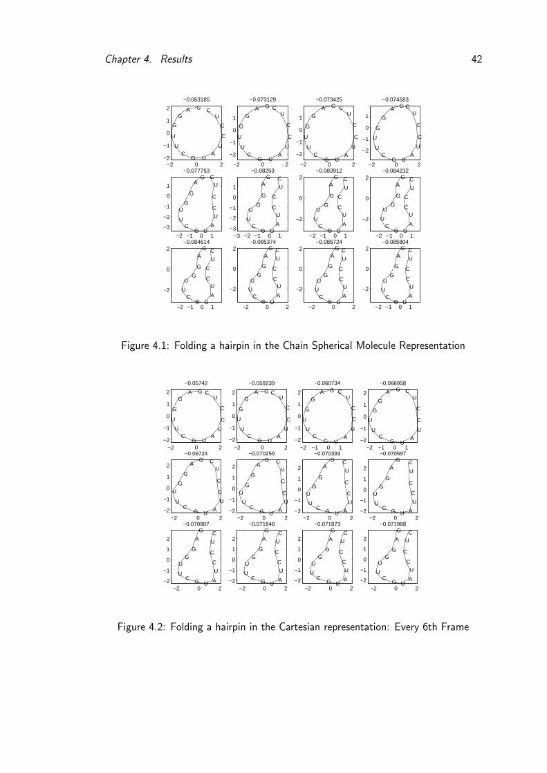
4.1 Folding a hairpin in the Chain Spherical Molecule Representation 42
4.2 Folding a hairpin in the Cartesian representation: Every 6th Frame 42
4.3 Adjusting parameters of almost correct hairpin . . . . . . . . . . . 43
4.4 Comparing structure under initial parameter settings and learnt
parameters . . . . . . . . . . . . . . . . . . . . . . . . . . . . . . . 44
4.5 Comparing the Energy of a Line against the Hairpin . . . . . . . . 44
4.6 Comparing the hairpin under intitial perturbed parameters and
learnt parameters . . . . . . . . . . . . . . . . . . . . . . . . . . . 45
4.7 Adjusting parameters for the hairpin from initially perburbed pa-
rameters . . . . . . . . . . . . . . . . . . . . . . . . . . . . . . . . 46
4.8 Adjusting Parameters of a Hairpin starting from perturbed param-
eters . . . . . . . . . . . . . . . . . . . . . . . . . . . . . . . . . . 47
4.9 Individually folding a molecule from the main sample . . . . . . . 47
vi

List of Tables
1.1 Different Types of RNA . . . . . . . . . . . . . . . . . . . . . . . 6
1.2 Classifying the different levels of RNA structure . . . . . . . . . . 9
2.1 RNA Secondary Structures considered by MFold . . . . . . . . . . 15
3.1 Modelled base to base interactions . . . . . . . . . . . . . . . . . . 33
3.2 Starting values . . . . . . . . . . . . . . . . . . . . . . . . . . . . 34
A.1 Structure produced and learnt parameters . . . . . . . . . . . . . 57
B.1 Structure produced with motifs and learnt parameters . . . . . . . 61
vii

LIST OF TABLES 1
1280 10138 64063
Chapter 1
Introduction
1.1 Overview
The aim of this project is to determine the structure of an RNA molecule given
its sequence by using the knowledge gained from a database of sequences and
their real life structures.
ACCACGGUUCACAA
Figure 1.1: Structural determination given an RNA sequence
RNA is involved in many of the fundamental processes in life and there are
many scientific and medical reasons why determining RNA’s functions would be
very useful, where its function is determined almost exclusively by its structure.
Due to this, there has been lots of prior work in structural determination of which
little has come from a basis in inference and graphical models instead mostly using
ad-hoc methods.
To determine the correct structure, there needs to be a scoring function which
2

Chapter 1. Introduction 3
rates how well a structure fits a given sequence. It is then reasonably simple -
if computationally expensive - to find a structure which maximizes this scoring
function. This is a common optimization problem for which there exist lots of
techniques to tackle it.
The fundamental problem is how to design or create a scoring function that
is able to differentiate between what structures fit a sequence and so could occur
within a cell and what simply maximises the score but couldn’t exist in real.
Manually creating and tuning a scoring function which can tell between good
and bad structures is actually a very difficult problem. As the point is to get
structure which would actually occur within a cell, there are many interactions
which have to be taken into account which are hard to explicitly model, like the
effect of the surrounding water molecules.
This project on the other hand tries to make the real world structure for some
given sequence more likely. The scoring function is modelled as P (C | Ψ, seq),
the probability of the structure given the parameters Ψ and the sequence. Using
MCMC and gradient ascent, it is then possible to increase the likelihood of the
structure by adapting the parameters, which is done for all real world examples.
The hope is then that there a set of parameters which will correct score structure
for lots of sequences and will generalise to novel sequences.
The main results from this project are that it works well on trivial example
cases like a single hairpin or a simple 3d structure. However, it does not generalise
so well to optimising for multiple types of molecules at the same time.
1.2 What is RNA and Why Determine its Structure
1.2.1 What RNA is made of
RNA and DNA are both nucleic acids and consist of bases hanging off a sugar
phosphate backbone. RNA is the evolutionary older molecule, and it is thought
that it used to used to perform all tasks in the cell[10] which tend to be done
by proteins in modern cells, while DNA is a much more stable molecule used for
long term information storage. This means RNA has the potential to form lots

Chapter 1. Introduction 4
Images from http://www.ch.cam.ac.uk/SGTL/Structures/nucleic/backbone.html and http://www.tulane.edu/~biochem/nolan/lectures/rna/
images/rnaimage2.gif
Figure 1.2: Chemical structure of DNA
of useful structures with catalytic properties.
If the structure of RNA could easily be determined for an arbitrary sequence,
it should be possible to attempt to design RNA that carry out tasks in the cell
for which Proteins would be normally used. This would open up new avenues
of attack on lots of existing medical problems as it might be easier to use RNA
molecules than attempting to use proteins. Also it would be easier to work out
structure for existing RNA molecules within the cell and from that their function
within the cell.
The structure of the sugar phosphate backbone as well as the possible bases
can be seen in 1.2. y
According to the central dogma of molecular biology, a large part of what RNA
generally do within modern cells is to act as a disposable information distribution
system, unlike DNA which is used for long term storage and proteins that are
used as functional agents. Information only every travels one direction in modern
cells, with a few exception like virii. This can be seen in 1.3.
Even in modern cells, RNA is a very versatile molecule that performs many
different functions within the cell. For instance, here are the some of the main
types of RNA as can be seen in 1.1

Chapter 1. Introduction 5
Figure 1.3: Central dogma of biology - should I include this? should I cite it from
CBD notes?

Chapter 1. Introduction 6
RNA type Description
Transfer RNA
Small 80 base sequences of RNA that connect
to a amino acid and contain the anti-codon
of the triplet that code for that amino acid.
In effect it is a translation device from the
RNA sequence to a protein amino acid. These
are matched up during protein synthesis to
convert the sequence to a protein.
Image from http://www.cgl.ucsf.edu/home/glasfeld/tutorial/trna/trna.html
Messenger RNA
Generally a copy of the sequence of some DNA
that will be synthesised to a protein. Can also
fulfil the same actions as DNA, as it would
probably have to have done in proto-cells.
Ribosomal RNA
This form of RNA forms a complex with var-
ious proteins to form the ribosomes. These
are vital for translating mRNA to proteins.
Image from http://www.zib.de/MDGroup/rnalab/firstpageDateien/rRNA.html
Table 1.1: Different Types of RNA

Chapter 1. Introduction 7
This project should be able to determine the structure of all of them, as this is
a functional classification not based upon any differences in the RNAs underlying
structure.
1.2.2 What is DNA
The main difference between RNA and DNA is an OH instead of a H in the 3’
position on the sugar ring which means that the structure of DNA is a lot more
stable. There is also a different base T instead of U. This means that the project
should also be able to fold DNA molecules with only retraining and changing
internally the U base to a T base.
DNA have only relatively recently been found to have catalytic properties as
well[13] which means that this project might be able to find interesting structure
that DNA can form.
1.2.3 What are Proteins
Proteins are the modern work horses of the cell. They perform almost all of
the physical interaction to the outside of the cell and almost all of its internal
maintainance. Due to their shape and interaction with other molecules, they can
make and break bonds on other molecules overcoming the activation energy that
would be required. This makes them extremely powerful and a lot of work has
been done on attempting to determine their structure.
There are lots of similarities between structure determination in proteins and
RNA molecules. This means if the technique on RNA works very well, it should
also be applicable to folding proteins. This also means that there is a very large
base of literature on protein folding which can be referred back to as proteins
play a central role in modern cells and is also very important to medical science.
Protein structure determination has the advantage that it is that there exist
a lot more proteins with their structure determined than with RNA. This should
lead to less data scarcity problems but as proteins have more base units(20 amino
acids vs 4 different base types) this leads to 380 point to point interactions com-

Chapter 1. Introduction 8
pared to 12 point to point interactions in RNA to get data for.
1.2.4 Different levels of structure
The structure of RNA can be defined on different levels. Not all approaches to
finding the structure of RNA work on the same structural level, so it is important
to be clear which level of structure is being talked about.
This project only deals with Quaternary structure, which reduces to being
equivilant to Tertiary structure in the case of there being only one RNA molecule.
Proteins have analogous structure level classifications.
1.3 Mathematical Background
1.3.1 Probability and Sampling theory
Starting with the discrete case. There is a set of events, X and a mapping
P (x ∈ X) which tells us the probability of event x ∈ X occuring.
Given a probability distribution P(X), it should be possible to calculate prop-
erties of X, like its mean. The mean can be calculated by
mean(X) = E(X) =∑
x∈X
xE(X)
or in the general case:
E(f(X)) =∑
x∈X
f(x)E(X)
This is extended to the continuous case:
E(f(X)) =∫ X
f(x)E(X)dx
This can be approximated by taking sampling from P(X) and averaging their
results. In the limit, this should give the correct answer. If x1, ..., xn are inde-
pendent samples from P(X), then:
∫ X
f(x)E(X)dx = 〈f(x)〉P (X) ≈1
n
∑
xi
f(xi)P (xi)

Chapter 1. Introduction 9
Structure level Description
Primary A C C A G
The sequence of the RNA molecule - this is co-
valent bonding between the backbone units.
Secondary
C C C G
G G G C
U
A
Covalent Bond
Hydrogen Bond
Deals with “local” ordered structure via hy-
drogen bonding: strands + helices in proteins,
short helical regions in RNA. Equivalently the
list of base pairs that occur in the three dimen-
sional RNA structure.
Tertiary
The global structure of protein/RNA, mainly
driven by other bonds than hydrogen-bonds. As
can be seen above in the interactions between
different strands
Quaternary
The interaction of multiple RNA molecules.
Table 1.2: Classifying the different levels of RNA structure
Chapter 1. Introduction 10
This is a sampling approximation. This will converge to the correct answer
given enough independent samples.
1.3.2 The Metropolis Method
Metropolis sampling allows one to sample from a distribution where the partition
function is not known, i.e. a function which is proportional to the required
distribution is known. This often occurs in Bayesian statistics when applying
Bayes Theorem. Given P (evidence | model) ∝ P (model | evidence)P (evidence),
it is possible to sample from P (model | evidence)P (evidence), without having
to know anything about P (model). With these samples, it is then possible to
approximate E(f(X)).
This technique will be needed to approximate an essential and otherwise in-
tractable integral within a derivative to make the sequence given the structure
more likely which is the central part of this project.
How to perform metropolis sampling is outlined below:
1. Pick a starting point x
2. Add x to list of points
3. Pick y from P (y | x). This is generally a Gaussian centred on x with a
small variance.
4. if P (y) > P (x) or if U(0, 1) < P (y)P (x)
accept the point else reject it.
5. If point was accepted set update x to contain y otherwise leave x unchanged.
6. Add point x to list of samples
7. Go to Step 2.
The list of points can be used as a list of independent samples in equation ??
and will give the correct answer given enough samples. This can be shown by
using Markov Chains[14].

Chapter 1. Introduction 11
1.4 Other approaches considered
Originally, this project was going to be based on a graphical models approach
to folding RNA molecules, for instance as it was applied in [15] to determine
the amino acid alignemnt when the backbone was known. However - assuming
pairwise interactions - it is extremely difficult to find any structural indepedencies
within the tree.
If it is assumed that the folding start from a straight line, one can assume
that the end start to fold independently. However, this quickly start to break
down and is equivilant to a well know optimization(keeping neighbours list and
cutting off interaction).
1.5 Temporal issues
What is the difference between folding RNA and determining its structure? It
is how much can be said about the evolution of the structure of the RNA as it
progresses towards its final shape. This project can not say anything about the
folding process of the molecule like for instance whether there are any plateaus
that would need to be crossed with a helper molecule. All that it can do is
determine the final structure.
While this project can model a complex that multiple RNA molecules could
form, it can’t for instance take into account how each RNA molecule would change
over the evolution of the interaction. An example of what this project can’t cope
with is an RNA molecule that cuts certain other RNA molecule in a specific place.
When this project refers to “folding”, it should be taken to mean the progres-
sion over time of deteremining the structure, not the actual states that an RNA
molecule would be expected to go through if it was actually folding in vivo.
1.6 Synopsis of the Rest of the Dissertation
Chapter two deals with previous approaches to this problem, their relative ad-
vantages and disadvantages and how they relate to this project while chapter

Chapter 1. Introduction 12
three details the methods that are used within this project and the implemen-
tation issues that were found. Chapter four goes into detail about how well the
algorithm performed and the results that were found an chapter five summarises
the achievements of this project and possible future extensions to this project.

Chapter 2
Literature review
2.1 Problem Feasibility of Structure Determination
of RNA and Proteins
What make this problem feasible to try and solve? There are a few conflicting
factors:
For:
• Some sucesses by Existing Techniques: Existing techniques in the field
lile Rosseta and MFold have been used for some time to sucessful help to
determine structures.
Against:
• Computational requirements: Despite the great advances in computa-
tional speed over the last few decades, simulating a small RNA molecule
with 2000 atoms and their interactions is still extremely computationally
difficult due to the scaling of the problem. The hope is that more intelligent
methods will get around this requirement.
• Helper proteins: Most proteins encounter energy plateaus during their
folding. This is where they are stuck in a sub-optimal folding that is a
local minima. Other proteins bind to the almost complete protein or RNA
13

Chapter 2. Literature review 14
molecule(?) and give it the required activation energy to complete its fold-
ing.
2.2 MFold
The traditional method that has been used when folding RNA is MFold that
only deals with secondary structure(see 1.2) in the hope that this provides a
significant step toward working out the actual Tertiary structure of the resulting
molecule. The scoring metric it uses is the amount of free energy available with
that structure using real life values worked out from experiments(?)
MFold works with the different types of loops of RNA, as can be seen in 2.1,
with tables of the reduction in free energy of having a loop of each type of each
size.
In this project these secondary structure are not modelled explicitly as the
energy function can encourage them to exist without explicitly knowing about
them. These will hopefully be reproduced in the results when real RNA is folded
and should be relatively easy to identify. It will prove interesting to compare the
results that MFold and this project return for the same molecule by looking for
overlap in the structure that they predict.
This prediction of the secondary structure can provide a starting point for
determining the full Tiertary structure of a given RNA molecule. The initial
shape can be resonably close to the real shape of the RNA molecule with only
the tiertary interaction wrong. However, this project is more interested in being
able to determine the structure of RNA where mfold fails and so starting from the
mfold starting position will lead to the wrong minima which might be difficult to
get out of. In effect, it could hinder more than it helps so it is not implemented.
2.2.1 Relative advantages and disadvantages
MFold has various advantages and disadvantages relative to this project:
• Bounds on folding time: As MFold uses dynamic programming methods,

Chapter 2. Literature review 15
Loop type Diagram Description
Bulges Bulges result form
small insertions or
deletions in a series of
base pair matches.
Hairpin Hairpins allow the
structure to flip back
on itself. They gener-
ally have a minimum
size of around 4-5.
Interior Very much like a
bulge except that a
mismatch occurs on
both sides.
Multi-loop Generally a central
feature in RNA.
Images from http://www.daimi.au.dk/~schauser/genome_analysis_F03/lectures_F03/RNA-struct-prediction.pdf
Table 2.1: RNA Secondary Structures considered by MFold
Chapter 2. Literature review 16
it can give low order polynomial bounds of time and space needed to fold
the RNA molecule.
• Gives solutions under constraints: Certain base pairings can be pre-
specified to occur in the solutions. If for instance it is known from exper-
imental data that a certain pairing must occur, MFold can ensure that all
solutions contain that pairing.
• Produces multiple solutions Unlike for instance a recursive approach
which would only give a single solution, MFold can produce multiple low
energy solutions to a problem [7]. This is useful as one of the other minima
may be the actual real life solution instead of the global minima. This
project should also be able to do this, but not in such a controlled manner.
• Gives estimates of real-life energy values: MFold actually takes into
account the measured energy of these configurations, while this project just
uses relative values which have little real life relevance.
Its main disadvantages compare to this project are:
• Only second order: As MFold only deals with secondary structure, it
can be almost completely wrong about the resulting shape of the molecule.
This project should be able to deal with this.
• Can’t deal with exception: Everything in biology has exceptions, and
base pairs are themselves not always immutable. For instance: Base triples
can form and pseudo-knots can form which are ignored, which are unpre-
dictable in how much energy they contribute to the final structure [9]
• Can’t deal with multi-stranded RNA: This is also related to the sec-
ondary structure constraint. This project should be able to deal with de-
termining the final shape that the multi-stranded RNA folds to.

Chapter 2. Literature review 17
2.3 Rosetta
Rosetta is the current hot topic in protein structure determination as it performed
extremely well on unseen data(CASP4 + CASP5). Part of this project is to look
into see how applicable its techniques are to determining RNAs structure.
The best possible situation for this project would be to be able to say that this
project is simply a more disciplined version of Rosetta, as there are similarities
in the approaches taken but with Rosetta should need more hand tuning.
The basis of Rosetta is the fact that the local structure influences but doesn’t
totally determine the final structure [3]. This can be seen by clustering together
fragments of sequences based on the similarity of their resulting structure.
There are three novels items in Rosetta: its scoring function, its searching
algorithm and its processing of its results.
2.3.1 Scoring function
The Rosetta scoring function is based on the decomposition: P (structure |
sequence) proportional to P (sequence | structure)P (structure), where P (structure |
sequence) represents sequence dependent features and P (structure) represents
universal sequence-independent features like β-strands assembling into β-sheets[1].
This decomposition can easily be seen to hold by use of Bayes Theorem:
P (Hypothesis | Evidence) = P (Evidence|Hypothesis)P (Hypothesis)P (Evidence)
. Bayes Theorem of-
fers a concrete way to establish probabilities which can otherwise be very difficult
to measure and plays a central role when applying probably theory to any statis-
tical problem.
P (Sequence | Structure) is approximated to two first order terms:
P (aa1aa2...aan | X) =∏
i
P (aai | X)
︸ ︷︷ ︸
∏
i<j
P (aai, aaj | X)
P (aai | X)P (aaj | X)︸ ︷︷ ︸
...
Penv Ppair
where Penv is the per amino acid environment term and Ppair is a pairwise
interaction term. Higher order terms were found to have little discriminative
power and so were not used.

Chapter 2. Literature review 18
XH20
H20
H20
H20
H20
H20
H20
H20
H20
H20H20H20H20H20
H20
H20
H20
H20
H20
H20
H20
H20
H20
H20H20H20H20H20
X
Example of a buried base Example of an unburied base
Figure 2.1: Buried vs non-buried Penv terms in Rosetta
Penv looks at each amino acid individually based on whether it is surrounded
by lots of other bases. This insures that hydrophobic terms tend to move to
the middle of structure whereas polar, hydrophilic terms to outside. This is very
important in protein structure determination, but not as relevant in RNA folding.
Ppair accounts for specific pair interactions between protein bases. It tends to
decay to 0 at 12A and thus can be ignored for long distances.
Penv and Ppair are set from looking at existing proteins and seeing what the
posterior distribution is. This project could attempt to derive these parameters
automatically.
This leaves the P (Structure) term. This is evaluated in terms of the secondary
structure, independent of the sequence and is chosen to give the maximum dis-
criminating power between real proteins and proteins that appear good under
normal scoring functions and P (Structure | Sequence) criteria but turn out to
be implausible. This was looked into by generating large numbers of non-native
proteins that scored very highly and plotting native vs non-native for each term
of interest.
Rosetta sets part of this term by representing every two residue segment in
the secondary structures by a vector and whether it is a helix or a strand. The
distances and orientations are then mapped onto spherical co-ordinates and were
examined manually looking for good classification performance between native
and compact but non-native structures, where a near native structure would still
score well. This approach resembles boosting[6], in that it allows focusing on the

Chapter 2. Literature review 19
mis-classified elements(the hard cases) and then combining various weak classifies
at the end.
Various other scoring methods were also used to score the proteins, whereupon
linear regression to find weights which produce the best classification performance
in predicted whether a protein is native. This weights are roughly equivilant to
the parameters Ψ used in this project and should be automatically be determined.
2.3.2 Sampling of the Protein Space
The basis of the sampling is the observation that the local sequence influences
the local structure, even if it doesn’t completely determine it. Rosetta stores the
proteins in a torsional space representation[4] to minimize the degrees of freedom
which are irrelevant to this problem.
Rosetta looks up all possible 3 and 9 residue segments are looked up for what
local structure they correspond to in a protein sequence database using sequence
profile comparison method which is nearest neighbours [2].
Nearest neighbour is used to find the 25 best sequences from the database,
where best is computed as distance between frequency of amino acids in each
sequence position.
A move then consists of substituting the torsional angles of a randomly chosen
neighbour at a random position for those of the current configuration.
This space is then searched using MC methods with energy functions that
favour compact structures with paired β-strands and buried hydrophobic residues,
see the scoring function.
2.3.3 Result processing
Each query repeated lots and lots of different times from different places. Results
are again clustered, and the centres of largest clusters taken as highest confidence
models, with the spread of the cluster being an indication of how reliable the
results are.
Another important point is that they used clustering on the resulting struc-

Chapter 2. Literature review 20
tures from the folding. The biggest clusters with the highest energy where then
submitted to the competitions as the possible folding of the protein as multiple
entries are allowed.
2.3.4 Relative Advantages and Disadvantages
Rosetta’s main advantages relative to this project are:
• Known to work well: Rosetta is known to perform very well on unseen
data, while this projects performance is very much unknown.
• Can work with constraints: Rossetta not only does ab initio predicition
of RNA folding but can also use experimental evidence that constrains the
final structure like Residual Dipolar Coupling [5]. This project can not
incorporate constraints like this although this could be incorporated into
the energy function.
Its disadvantages are:
• Manual tuning: It can’t automatically tune its parameters to fit the
data. Manual intervention is required. This project should be able to do
this automatically.
• Ad hoc: It is rather based on ad-hoc methods in places, like for instance
using linear regression to combine together lots of different
Its similarities
• Unit-less values: Both projects use non-real world values for energy
• Not physical modelling: Both projects do not explicitly model the un-
derlying physical processes but attempt to determine the structure using
other methods.
• Temporal issues: Both project determine the structure but can not de-
termine it progression over time as it reaches the final state.
Chapter 3
Methodology
3.1 Techniques used
3.1.1 Why use Probability Theory
Using an energy function to score the different structure available for a sequence
is not very powerful, as none of the machinery of probability theory can be bought
to bear upon it.
For instance, there is a sequence seq and structure C. The problem is to
make the structure C more likely for the sequence seq: Even the statement of
the problem uses probability theory. Simply increasing the score of the structure
by changing the scoring function isn’t good enough, as there is no guarantee that
all other structure aren’t increasing in some way, etc. While this could be done
in an ad-hoc way, it is better to use the natural and intuitive machinery that is
already there.
3.1.2 Defining P (C | Ψ, seq)
The probability function is defined in terms of the energy function. The energy
function must have continuous, differentiable parameters Ψ which will be adapted
to make the energy function prefer real structures for a sequence. Given that there
is an energy function H(C,Ψ, seq) where C is the structure, Ψ is the parameters
21
Chapter 3. Methodology 22
of the energy function and seq is the sequence of the RNA molecule, there is a
standard way to define a probability distribution:
P (C | Ψ, seq) =e−H(C,Ψ,seq)
Z
where Z is the partition function which turns it into a probability distribution.
This is needed so that P (C | Ψ, seq) satisfies the basic axioms of probability,
namely the continuous equivilant of that events must have a probability that
sums to one. It is defined as follows:
Z =∫
e−H(C,Ψ,seq)dC
Z is set of by the values of the parameters Ψ but is intractable to compute
in all apart from the most simply cases. However, using Markov Chain Monte
Carlo methods, it is still possible to increase the probability of a structure given
a sequence.
The energy function that is used in this project is defined in 3.3.1
3.1.3 Increasing the Probability of a Structure for a Given
Sequence
This is the central idea used within this project. As log is a monotonic function,
increasing log(f) is equivalent to increasing f. If this insight is applied to P (C |
Ψ, seq):
∂
∂Ψln (P (C | Ψ , seq)) =
∂
∂Ψln
(
e−H(C,Ψ ,seq)∫
e−H(C,Ψ ,seq)dC
)
= −
(
∂
∂ΨH (C,Ψ , seq)
)
+
∫(
∂
∂ΨH (C,Ψ , seq)
)(
e−H(C,Ψ ,seq)∫
e−H(C,Ψ ,seq)dC
)
dC
= −
(
∂
∂ΨH (C,Ψ , seq)
)
+
⟨
∂
∂PH (C,Ψ , seq)
⟩
P (C,Ψ ,seq)
Markov-chain Monte Carlo is used to approximate⟨
∂∂PH (C,Ψ , seq)
⟩
P (C,Ψ ,seq).
As it is not possible to evaluate P (C | Ψ, seq), simple gradient ascent is used
to try to find the local maxima:

Chapter 3. Methodology 23
Ψn+1 = Ψn + stepsize ∗∂ lnP (C,Ψn, seq)
∂Ψ
If stepsize is small enough and this equation is iterated often enough it should
increases P (C | Ψ, seq) by changing Ψ until it is a local maximum. Now if an
attempt was made to find the structure of seq by maximizing P (C2 | Ψ, seq), it
should hopefully find that C = C2, i.e. the structure that was earlier made likely.
This has a nice side effect of having an semi-intuitive explanation - if(
∂∂ΨH (C,Ψ , seq)
)
=⟨
∂∂PH (C,Ψ , seq)
⟩
P (C,Ψ ,seq)
then it has converged. If they are not equal, Ψ is adjusted so that ...
A simple approach is taken to try and optimise for multiple molecules at the
same time: This equation is iterated for each molecule in turn. This is repeated.
There are no guarantees of convergence without arbitarily small step size
and infinite precesion or of being able to find parameter setting that satisfy the
requirements for multiple molecules at the same time.
3.1.3.1 Reducing the Burn-in period for MCMC
One important consideration is what structure is used to start the MCMC sam-
pling from. Just starting from a straight chain can bias the sampling as it is in a
area of very low probability and the MCMC will take a long time to find an area
of higher probability, which it would normally be present in. This time is called
the burn in period and sample point from this time are generally discarded or
this bias can be avoided by either having very long sampling periods.
The approach taken in this project is to start with the shape that which
should be made more likely, then maximise its probability for a sufficiently long
period until a local minima is reached. Then after every time the parameteres
Ψ are updated perform a few more cycles of minimising the energy to ensure
that the starting position tracks the changing local minima. This was found to
significantly reduce the numbers of cycles of MCMC sampling that had to be
performed.
Another consideration is whether to use all sample or just to record a sample
from this stream occasionally in the hope of getting overall independent samples.
Chapter 3. Methodology 24
The advantage of getting independent samples is that it allows estimates of the
number of samples required, but when and how often to record to ensure this [14]
3.1.3.2 Other possible kinds of sampling
Gibbs sampling could also have been implemented. Gibbs sampling works by
sampling first variable given all the others, then the second variable given all the
others etc. Its main advantage over MCMC is that every sample is accepted and
no samples are lost due to rejection.
A continuous solution would be intractable but by discritizing each variable
in turn and evaluating it in every position, it is then simple to normalise these
and turn them into a valid distribution but this is going to be a lot more work
than simply throwing away the samples in Metropolis sampling.
Hybrid Monte Carlo sampling was also looked at, but it was decided that it
was too slow. For a more complete survey of other available sampling methods,
look at [14].
3.1.4 Finding the Structure given the Sequence of an RNA
Molecule
As the mapping from the energy to the probability is anti-monotonic, maximising
the probability is equivalent to minimising the energy function. All the deriva-
tives of the energy function with respect to the structure can be calculated, so a
standard function minimisation routine namely conjugate gradient descent from
netlab[?] is used to optimise the structure with the given sequence and parameter
settings.
So, given a sequence seq an initial shape is chosen for the structure C like a
circle or a random structure. The parameters settings Ψ are known from either
setting them manually or from being adapted for a certain shape as done in the
last section.
Convergence is not explicitly detected as sometimes it can appear to have
converge but then “break through” to another local minima and start improving

Chapter 3. Methodology 25
the structure again. This project takes a simple approach and just attempts to
optimise the energy function for a long time, making up for the slowness of this
approach by simply using more computers.
3.1.5 Rossetta-style Simulated Annealing to find all Minima
The main problem with just using the technique outlined above it is a naıve
hill climbing algorithm so it will never find more than one minima. The energy
function can easily have multiple minima of which one is the RNA molecules.
Starting from random positions is one approach to this problem but one which
is unlikely to find all the different minima and there are many highly twisted
minima when the molecule is overlapping a lot. Instead a simulated annealing
style approach modelled on MCMC simulated annealing as in Rosetta [2] is used
to try and find all of the minima.
Each update is to select a random position on the RNA molecule. Then
copy three sets of bond lengths, bond angles and torsion angles from a randomly
selected fragment with the same sequence.
The probability of a structure given a sequence is updated in this context to
take into account the temperature:
P (C | Ψ, seq) =e−H(C,Ψ,seq)
Z ∗ T
This means that the higher the temperature, the more likely it is that a jump
which decreases the probability will suceeed. When the temperature decrease,
it becomes harder and harder to do big jumps, at which point the conjugate
gradient descent method is used to find the final maxima.
3.2 Modelling the Structure of the RNA Molecule
3.2.1 Why use a High Level Molecule Representation
The RNA molecule is stored at a high level representation; only the position of
base is stored, not the positions of all of the atoms that make up that base. This
is done for many reasons:

Chapter 3. Methodology 26
• In order to make the problem more tractable in the short time frame avail-
able.
• To very significantly the reduce the computational complexity of trying to
fold the molecule. As there are about 20 atoms per base at least point to
point interactions between all molecule have to be taken to account makes
the problem run a few orders of magnitude quicker
• It is a more elegant solution to the problem that is more likely to be applied
to other problems as it requires less prior knowledge. For instance to adapt
this project to DNA folding, all that would be required is changing all U
bases to T bases and retraining, while with a atom based system the actual
structure would have to change. While this might be minor, adapting to
prxotein folding would certainly require almost a complete rewrite, while
with a higher level representation it would only require adding more bases.
The speed and result of the structural determination depends on how the that
is found can be folding specific, various different representations of the positions
of the RNA bases can be used. The current implementation supports 3 different
kinds of representations where the main difference is how many irrelevant degrees
of freedom can be explicitly ignored in the representation and how long it takes
to calculate the derivatives.
It would be expected that the time taken to determine how long it takes to fold
a structure would be a trade off between converging faster in representation where
it can ignore irrelevant degrees of freedom versus the trade off of the derivatives
being slower to calculate.
3.2.2 Cartesian ’xyz’ Molecule Representation
The representation is simply Cartesian co-ordinates of each base.
C = (x1, y1, z1), (x2, y2, z2), ..., (xn, yn, zn)
The main advantage of this representation is the speed with which it can be

Chapter 3. Methodology 27
moved with as when calculating the derivatives it requires only an update to 2
different sets of parameters, unlike with say chain spherical.
∆1,5 =√
(x1 − x5)2 + (y1 − y5)2 + (z1 − z5)2
Then for example:
d∆1,5
dx1=
x1 − x5
Delta1,5
All points individually effect the structure. However translating or rotating
all points will not affect the structure or its probability so there are 6 degrees of
redundancy within the representation.
3.2.3 Chain Spherical ’rtp’ Molecule Representation
Each base is described in spherical co-ordinates relative to the last base as can be
seen in Figure 3.1 without any rotation. Each base then uses normal non-rotated
Cartesian co-ordinates to determine the relative distance to the next base. r1, θ1
and φ1 specify the location of the first base relative to the origin. This means
that the chain spherical representation can represent any Cartesian molecule in
any position, which is useful for debugging.
So the structure is defined as follows:
C = (r1, θ1, φ1), (r2, θ2, φ2), ..., (rn, θn, φn)
To convert to Cartesian:
x1 = r1 cos(θ1) sin(φ1) y1 = r1 sin(θ1) sin(φ1) z1 = r1 cos(φ1)
x2 = x1 + r2 cos(θ2) sin(φ2) y2 = y1 + r2 sin(θ2) sin(φ2) z2 = z1 + r2 cos(φ2)
x3 = x2 + r3 cos(θ3) sin(φ3) y3 = y2 + r3 sin(θ3) sin(φ3) z3 = z2 + r3 cos(φ3)
... ... ...
and to convert back:
r1 =√
x21 + y21 + z21 θ1 = arctan y1, x1 φ1 = arccos z1r1
r2 =√
(x2 − x1)2 + (y2 − y1)2 + (z2 − z1)2 θ2 = arctan y2−y1x2−x1
φ2 = arccos z2−z3r2
... ... ...

Chapter 3. Methodology 28
y
x
z
θ1
r 1
r 2
z
y
x
φ1
r
φ
θ
2
2
2
3
x
y
z
Figure 3.1: Chain Spherical co-ordinate system
In this representation, r1, θ1 and φ1 do not in any way affect the actual struc-
ture of the molecule or its probability, so these can be ignored when attempting
to find the local minima. The final structure can still be rotated in 3 different
ways, so there are still 3 implicit degrees of redundancy with the representation.
As r1, θ1 and φ1 can be ignored when folding the molecule, it should converge
faster than the Cartesian representation. However, it is more expensive to calcu-
late the derivative of a point to point interaction. It requires updating on average
n/2 other bases, instead of just 2.
3.2.4 Bond and Torsion angle based
This representation stored the bond lengths, bond angles and torsion angles of
the chain. This is a very natural representation for the molecule as this relates
closely to the constraints that a real chemical model has to satisfy.
The derivatives for this are more complex and were not computed. Instead,
for completeness they were simulated with numerical approximations to check if
the resulting folding was any more complete, but no noticeable difference was
found.

Chapter 3. Methodology 29
G
A
A A
A
C G
A
A A
A
C1
2
3 4
5
6
Updates to bring GC bases closer to-
gether in Cartesian representation
Updates to bring GC bases closer to-
gether in Chain Spherical representa-
tion
Figure 3.2: Updates required in Cartesian Representation vs Chain Spherical
In this representation,
r1
bondangle1 bondangle2
torsionangle1 torsionangle2 torsionangle3are all the parameters that don’t affect the probability of the structure. After
removing these from consideration, there are no implicit redundant degrees of
freedom left, i.e. there is no simply way to change all the points that don’t affect
the energy function.
However, this comes at a high computational cost, as calculating each deriva-
tive of a point to point interaction is made considerably more expensive and
complicated.
3.2.5 Data preprocessing
The data that this project uses is pulled from various internet databases of RNA
structure files. This project uses [16] and then processes the data which is re-
trieved with various perl scripts.
When loading a RNA molecule in which RNA is stored as atom positions, the

Chapter 3. Methodology 30
mean of all atoms belonging to a single base are averaged to get a final position
for the whole molecule instead of for instance picking the same position on the
backbone every cycle.
In order not to bias the results, no sequence is allowed to have more than
one structure. If there are more than one structure for a sequence, the structure
is picked randomly from the options available. This is because there are often
duplicate entries in the database or entries done in very slightly different condi-
tions. However these don’t pose very a interesting challenge for this project as
first the rather larger question of whether it can get the general structure of the
RNA molecule should be answered.
3.3 Defining the Energy function
3.3.1 Requirements
As already mentioned, the parameters Ψ of the energy function must be continous
and differentiable in order that the technique that is used to make structure more
likely actually works. If for instance the parameters Ψ were discrete, another
technique like genetic algorithms would have to be applied.
The energy function is based only upon distances between different bases is
due to the multiple ways to represent the RNA molecules, as can be seen in the
last section. It is not clear that having non-distance terms would increase the
expressive power of the energy function but if there was any terms that would be
more useful not expressed in terms of distance, it would be very easy to implement
them.
3.3.2 Scoring the bonds between neighbours
The energy function needs to constrain bonds between neighbours in the chain
as bases can only be a certain distances apart and can only be at certain angles
to each other due to the underlying chemical structure. These constraints on the
bonds are generally expressed in terms of their length, bond angle and torsion

Chapter 3. Methodology 31
ACCACGGUUCACAA
Figure 3.3: Expressing bond preferences of sequential bases in terms of distance
angle. This project maps these constraints to distance based constraints. The
mapping from length, bond angle and torsion angle to distances can be seen in
3.3.
As each base has a difference chemical structure, it can be assumed that there
is a base specific term to the distributions of bonds, so the local structure is
constrained by the local sequence.
This leads to the beginning of an energy function:
H(C,Ψ, seq) =∑
i
αBL
n
(∆i,i+1 − pbsmeanseq(i,i+1))
2
pbsσseq(i,i+1)+αBA
n
(∆i,i+2 − pbsmeanseq(i,i+1,i+2))
2
pbsσseq(i,i+1,i+2)+
αBT
n
(∆i,i+3 − pbsmeanseq(i,i+1,i+2,i+3))
2
pbsσseq(i,i+1,i+2,i+3)
∆i,j is the Euclidean distance between bases i and j. There is no need to
normalise the gaussian distrbution used as this is the energy function. This
normalising occurs when converting to P (C | seq,Ψ) and the relative strength
learned from the real data and this means that energy function is more simple
which is an advantage as it will be evaluated a lot.
pbsmeanseq(i,i+1) is the mean of the bonds lengths that occur and pbsσseq(i,i+1) is
the standard deviation of that bond. These are simply set by looking at every
sequence fragment which the sequence seq(i,i+1) occurs and taking the mean and
standard deviation of ∆(i, i+ 1) through all the data that is available.
The parameters Ψ that are as defined as yet are αBL, αBA and αBT . αBL
models how important it is that the bond length being close to the mean for
those pair of basis seq(i, i+1), taking into account how much variance is naturally
within the bases. αBA and αBT do the same for bond angles and bond torsionl.
As there are so many pbs values, these are set directly from the database

Chapter 3. Methodology 32
instead of trying to learn them from the examples. These are very unlikely to
change much and it reduces the complexity of the learning problem.
In order to model multiple RNA molecules, this project models a single long
molecule but discounts the local bond constraints over the boundary to a different
actual RNA molecule which in essence allows modelling of multiple strands for
free. This means that the final energy function is:
H(C,Ψ, seq) =∑
i
αBL
n
(∆i,i+1 − pbsmeanseq(i,i+1))
2
pbsσseq(i,i+1)+αBA
n
(∆i,i+2 − pbsmeanseq(i,i+1,i+2)
2
pbsσseq(i,i+1,i+2)+
αBT
n
(∆i,i+3 − pbsmeanseq(i,i+1,i+2,i+3)
2
pbsσseq(i,i+1,i+2,i+3)
where Si,j is 1 if base i is on the same molecule as base j and 0 if not.
3.3.3 Incorporating Base to Base interactions
There are various interactions between bases that should be modelled as can be
seen in Table 3.1.
The α and C values are all in Ψ, the parameters of the energy function. The α
values are to be able to adjust the relative importance of each of the interactions,
while the C values allow adjusting how close the bases have to be. For instance,
it would be expected that CKD would be low as this it is always important that
base pairs do not overlap.
This give the complete energy function:
H(C,Ψ, seq) =∑
i
αBL
n
(∆i,i+1 − pbsmeanseq(i,i+1))
2
pbsσseq(i,i+1)+αBA
n
(∆i,i+2 − pbsmeanseq(i,i+1,i+2)
2
pbsσseq(i,i+1,i+2)+
αBT
n
(∆i,i+3 − pbsmeanseq(i,i+1,i+2,i+3)
2
pbsσseq(i,i+1,i+2,i+3)+
∑
i,j
−α2GCn2
MGCij
∆i,j + C2GC−α2AUn2
MAUij
∆i,j + C2AU−α2GUn2
MGUij
∆i,j + C2GU
−α2UMn2
MUMij
∆i,j + C2UM−α2LSn2
MLSij
∆i,j + C2LS−α2KD
n2MKD
ij
∆i,j + C2KD
where S are the parameters of the chain, and P are the parameters of the
energy function.

Chapter 3. Methodology 33
Energy Term Description
−α2GC
n2
MGCij
∆i,j+C2GC
G and C bases form strong triple hydrogen bonds and so
should be encouraged to come closer together. This is
done by subtracting this term from the energy function
which means that the closer each pair of G and C bases
are, the lower energy the final molecule is. MGCi,j = 1
everywhere that base i is G and base j is C or visa versa.
−α2AU
n2
MACij
∆i,j+C2AU
A and C bases form double hydrogen bonds and so should
also encouraged to come close together. MAUi,j is 1 every-
where that base i is A and base j is U or visa versa.
−α2GU
n2
MGUij
∆i,j+C2GU
G and U bases form a hydrogen bonds and so should also
be encouraged to come close together. MGUi,j is 1 every-
where that base i is G and base j is U or visa versa.
+α2UM
n2
MUMij
∆i,j+C2UM
UM stands for unmatched. Bases which are not comple-
mentary should be kept apart as no base pairs can form.
MUMi,j is 1 everywhere that base i is not complementary to
base j.
−α2LS
n2
MLSij
∆i,j+C2LS
LS stands for long stem matches is designed to encourage
long sequence of matching base pairs to come together.
This is explained in more detail below.a
z+α2KD
n2
MKDij
∆i,j+C2KD
KD stands for the Keep Distance. This is designed simply
to stop bases getting too close together or even overlap-
ping. All entries of MKD apart from the diagonal are set
to 1.
Table 3.1: Modelled base to base interactions

Chapter 3. Methodology 34
Parameter αBL αBA αBT αGC αAU αGU αUM αLS αKD CGC CAU CGU CUM CLS CKD
Initial Setting 1 1 1 3 2 2 2 1 2 .2 2 3 2 1 0.15
Table 3.2: Starting values
The conversion from energy function to a probability distribution is done:...
Thermodynamics tell us that the folding is a probability distribution proportional
to the exponent of the energy function[8].
The reason that point-wise interactions are divided by n2 while the sequential
constraints are only divided by n is to ensure that the interactions strengths are
relevant to molecule of different lengths.
3.3.4 Initial Parameter Settings
Starting values were set to αGC = 3αGU and αAU = 2αGU to account for the
number of hydrogen bonds that form when the base pairs match up and thus
their relative desirability. The other values were initally guess at, with the hope
that it would be close enough to the real answer so it could learn the rest. The
full set of starting values used can be seen in Table 3.2.
3.4 Incorporating common motif recognition
While the basic folding worked well enough, a second approach was tried to make
more use of the data available. [3] found the existance of recurring sequence
patterns that cross over protein family groups. Simple motif recognition is in-
corporated into this project in order to try and improve the performance of the
structure determination algorithm and to test if the equivilant observation holds
about recurring RNA bases.
3.4.1 Choosing motifs
Given the length of motifs n that should be searched for:

Chapter 3. Methodology 35
1. List all fragments of length n on every molecule within the database.
2. Group all fragments with the same sequence, discarding sequences with only
one fragment.
3. Pick out the fragements with the highest simularity between their structures
(See Section3.4.2)
4. Add the best motifs to the energy function with an extra parameter to
indicate their relative importance.
3.4.2 Comparing structures
Originally the structure were compared by converting to the distance, bond angle
and torsion angle representation then taking a simple distance measure between
the structure to be compared. This was highly unsatisfactory for many rea-
sons like the complexity of ensuring that the angle measurement correctly looped
around, the fact that it doesn’t generalise well to comparing more then two dif-
ferent motifs etc. It also provided misleading results about how well the project
was working that lead to lots of time being wasted.
The second approach that was taken was to measure the mean of the standard
deviation of each element of ∆ for each sequence. ∆ for molecule k is defined as:
∆ki,j =| C
ki − Ck
j |
The structure simulatity measure is then:
1
n4
n∑
i,j
(m∑
k
(∆ki,j − ( 1
m
∑mk ∆k
i,j))2
m− 1
While this takes O(n2) to evaluate, its simplicity means that it less likely to
be mis-implemented and more likely to give a correct answer.
Chapter 3. Methodology 36
3.5 Implementation Issues
3.5.1 Development Environment and Language
Initially development started in octave[17], however due to various annoyances
with this language development was moved onto matlab. Matlab was used for
speed of development which is important in a project with a short timescale. It
deals very well with numerical exceptions like dividing by 0, has good debug-
ging facilities, generally highly numerically accurate due to good libraries and
performance is good if the code is properly vectorized and/or compiled.
Netlab[12] is a very useful library of matlab functions to perform various nu-
merical tasks which proved invaluable. This project especially used the conjugate
gradient descent implementation and the gradient sanity checking code with some
minor modifications.
Matlab had in relation to this project serious problems with the number of
licenses running out when attempting to cluster the software. If given more time,
a port to a licence free language would be a very good idea. As the matlab
compiler can produce C code, it shouldn’t be too hard to integrate the resulting
compiled to C code into a Beowulf cluster using MPI.
Some of the glue code needed was built using the computer equivalent of duct
tape: Perl. This was mainly used to parse the databases of sequences online due
to its strength in text processing and to process equations outputted from Maple.
Revision tracking control was provided by CVS. This was used to insure that
the same code-base on multiple computers was matched up as a personal com-
puter was used to process the database and to be able to tag releases to keep
track of milestones achieved.
The development environment used was Emacs running in octave mode, with
the text mode version of matlab. This was found to be the most productive
method due to the occasionally instability of the Java interface to Matlab.

Chapter 3. Methodology 37
3.5.2 Regression checking
With any project it is important to be able to trust the results that it gives back.
This project has regression checking built in as various sanity checking function
that make sure the routines are giving back correct answers.
For instance, all derivatives that are computed within this project can be
rechecked numerically to check for any bugs in either the derivation or the im-
plementation. This proved to be highly useful when building the project.
3.5.3 Vectorization, Optimisation and Benchmarking
Most of the coding was initially written unvectorized for simplicity. It was then
vectorised for simplicity and extra speed. This provided most of the speed up.
The other main optimisation used (which was considerably less effort) was to
use the builtin matlab compiler. Overall the code ran twice as fast.
A specific folding case was used everytime to give fair comparisions of the
speed at this project could fold the RNA molecule.
3.5.4 Parallelizing the code
Various possible clustering methods were looked into, including plab[11] NetSolve
and hand-coding to Beowulf with MPI. Plab was used for speed of development
and the fact that almost all of the problem are ’embarrassingly parralizable’.
A brief attempt was made to port plab to octave as it would solve the problem
of only limited number of licenses being available for matlab within the Univer-
sity of Edinburgh. However lack of non-blocking I/O routines and bugs within
the blocking IO routines within the octave libraries meant that this had to be
abandoned.
There are many parts of the code that were parallelizable:
• Independently folding the same molecule to see if different local minima are
found with simulated annealing.
• Many small runs of MCMC instead of one big one run.

Chapter 3. Methodology 38
• When adjusting parameters, each molecule in the database can be consid-
ered separately, then the sum of their adjustments applied. This limits to
parralellism to a computer per molecule, but it is still a significant speed
up.
• When analysing the results, analysing each parameter setting is indepen-
dent, so it simply break up into work units which can be spread out.
3.6 Evaluating the Learning of the Parameters Ψ
Evaluating how well the parameters are adapted is not as trivial as it may at first
seem. For instance if we make some random sequences and folding them using
one set of parameters and then try to derive those parameters, there could be
many possible different settings which equate to the same set of local minima in
the energy function. A trivial example is double all the α parameters which will
result in a “colder” more extreme energy function gradient.
Three main evaluations were carried out: trying to fold an artificial example,
trying to derive the parameters of a random folding and attempting to fold real
data.
3.6.1 Initial Teething Problems
The computational expense of trying to repeatedly fold a complex model from
scratch for a sucession of slightly different parameter settings is prohibitively
expensive (compounded by the lack of matlab licenses) as many attempts may
have to be found to find the correct minima of the energy function, assuming that
it even exists. An efficient way to approach this problem is to start the folding
from the target structure as this ensures that the correct minima is always found.
As long as enough cycles of function minimisation is allowed to ensure convergence
to the true shape, the divergence from the initial this should acuratley reflect the
true performance of the algorithm.
However, in practice this turned out to be a very bad idea. As the folding

Chapter 3. Methodology 39
progresses, not only does the energy minima get closer to the shape that the
algorithm should be learning but also there is the equivilant of the temperature
decreasing in simulated annealing. 1. This is where the minimum of the energy
function get more and more extreme and the energy of these gets arbitiarily low
and the probability approachs one.
This would not normally be a problem but the netlab conjugate gradient
descent implemention that is used by this project uses a line search with a default
absolute accuracy of 10e-4. As the temperatre decreases, so does the ability of
the line search algorithm to progress around the energy landscape.
This means that the longer a run has been going on, the better it appears to
perform, indepedently of its actual performance. Needless to say, this was a bit
misleading and the sanity checking of running the folding for a very long time
didn’t help as each iteration was limited by the line accuracy.
All results that are present in the project have been folded from a circle to
ensure that there can be no bias due to this temperature change. This problem
was discovered late on in the project which combinded with the lack of matlab
licesnes is why there are less results than would be wanted for a perfect evaluation.
3.6.2 Learning an Artifical Hairpin Structure
A artificial hairpin was constructed, first in a very undisciplined manner. However
it was found that this hairpin was very unrealistic as the hairpin turn contained
to few bases. A more realistic model was made based on one of the loops of
Transfer RNA as can be seen in 3.4.
3.6.3 Random folding
A number of random sequences and random structures are generated, and then
“folded” with known random parameters setting. Using only the determined
structure of these sequences with all parameters reset to 1, test if the parameter
1The same things happens in the EM algorithm with a mixture of guassians where if a
Gaussian becomes centred on a single point, its variance gets arbitarily small, which is generally
a very bad model of the underlying data

Chapter 3. Methodology 40
−3 −2 −1 0 1 2 3
−0.5
0
0.5
1
1.5
2
2.5
3
3.5
4
4.5
C
U
C
C
U
A
U
G
C
U
U
G
G
A
G
Figure 3.4: Artificial hairpin based on loop of Transfer RNA
adaption routine can derive the correct parameter setting.
As the derived parameters may not necessarily be the same as the initial
paramteres but still be correct in being able to determine the correct structure,
we also have to test how close the determined structure for the random data is
to the initial folded structures.
3.6.4 Real data
Due to computational reasons, only a small subset of the complete dataset can
folded.
This will determine if the project would ever actually be useful for real worl
tasks in its present state and to highlight any specific problem with example
which it can not deal with.
This real data is folded both with and without motifs to investigate if they
help the molecule fold correctly.

Chapter 4
Results
4.1 Effects of Different Structural Repressentions
on Structure Determination
As predicted in Section 3.2.1, convergence is faster in the more advanced represen-
tations. Comparing the Cartesian molecule representation in Figure 4.1 against
the Chain spherical representation in Figure 4.2, there is an interesting qualita-
tive difference in how the molecule folds. It tends to curl around each bond more
which makes the straight lines more bendy, while the Cartesian tends to travel
more directly to the final shape, but take a lot longer.
The chain spherical representation works a lot faster even with its longer per
cycle evaluation time, as its about half as fast to evaluate but takes roughly 6
times as long to converge. Because of the speed difference, the Chain Spherical
RNA structure representation is used throughout the rest of this project.
4.2 Hairpin results
4.2.1 Adapting the Initial Parameter Settings
The first test of this project is to learn the structure of the artifical hairpin in
Section 3.4 for its sequence. Initially the parameters in 3.2 were used. Parameters
41
Chapter 4. Results 42
−2 0 2−2
−1
0
1
2 CU
C
C
UA
UGC
U
U
G
GA G
−0.063185
−2 0 2
−2
−1
0
1
CU
C
C
U
AUG
CU
U
G
GA G
−0.073129
−2 0 2
−2
−1
0
1
CU
C
C
U
AUG
CU
U
G
GA G
−0.073425
−2 0 2
−2
−1
0
1
CU
C
C
U
AUG
CU
U
G
G
A G−0.074583
−2 −1 0 1
−3
−2
−1
0
1
CU
C
C
U
AUG
CU
UG
G
AG
−0.077753
−3 −2 −1 0 1−3
−2
−1
0
1
C
U
C
CU
AUG
CU
UG
G
AG
−0.08253
−2 −1 0 1
−2
0
2 C
U
C
CU
AUG
CU
UG
G
AG
−0.083912
−2 −1 0 1
−2
0
2 C
U
C
CU
AUG
CU
UG
G
AG
−0.084232
−2 −1 0 1
−2
0
2 C
U
C
CU
AUG
CU
UG
G
AG
−0.084614
−2 0 2
−2
0
2 C
U
C
CU
AUG
CU
UG
G
AG
−0.085374
−2 0 2
−2
0
2 C
U
C
CU
AUG
CU
UG
G
AG
−0.085724
−2 −1 0 1
−2
0
2 C
U
C
CU
AUG
CU
UG
G
AG
−0.085804
Figure 4.1: Folding a hairpin in the Chain Spherical Molecule Representation
−2 0 2−2
−1
0
1
2 CU
C
C
UA
UGC
U
U
G
GA G
−0.05742
−2 0 2−2
−1
0
1
2 CU
C
C
UA
UGC
U
U
G
GA G
−0.059239
−2 −1 0 1−2
−1
0
1
2 CU
C
C
UA
UGC
U
U
G
GA G
−0.060734
−2 −1 0 1−2
−1
0
1
2 CU
C
C
U
AUG
CU
U
G
G
A G−0.066958
−2 0 2−2
−1
0
1
2C
U
C
C
U
AUG
CU
UG
G
AG
−0.06724
−2 0 2−2
−1
0
1
2C
U
C
C
U
AUGC
U
UG
G
AG
−0.070259
−2 0 2−2
−1
0
1
2C
U
C
C
U
AUGC
U
UG
G
AG
−0.070393
−2 0 2−2
−1
0
1
2C
U
C
C
U
AUGC
U
UG
G
AG
−0.070597
−2 0 2−2
−1
0
1
2C
U
C
C
U
AUGCU
UG
G
A
G−0.070907
−2 0 2−2
−1
0
1
2C
U
C
C
U
AUGC
U
UG
G
A
G−0.071848
−2 0 2−2
−1
0
1
2C
U
C
C
U
AUG
CU
UG
G
A
G−0.071873
−2 0 2
−2
−1
0
1
2C
U
C
CU
AUG
CU
UG
G
A
G−0.071988
Figure 4.2: Folding a hairpin in the Cartesian representation: Every 6th Frame

Chapter 4. Results 43
0 2000 4000 6000 8000 10000 12000 14000 160000
2
4
6
8
10
12
14
16
18ABTMGCcGCMAUcAUMGUcGUUMcUMLScLSKDcKD
Parameter αBL αBA αBT αGC αAU αGU αUM αLS αKD CGC CAU CGU CUM CLS CKD
Initial Setting 1 0 0 3 2 2 2 1 2 .2 2 3 2 1 0.15
Final Settings 16.3991 0 0 2.9135 2.1358 2.0676 1.9150 1.0056 1.9947 0.1842 2.0023 3.0283 2.0284 0.8794 0.0011
Figure 4.3: Adjusting parameters of almost correct hairpin
were adjusted as can be seen in Figure 4.3, but there was disappointingly little
imporvement as can be seen in Figure 4.4.
Overall the simularity matrix dropped from 0.0170 to 0.0134 which is a 24
Comparing the energy of the straight line with the energy of the hairpin can
be seen in Figure 4.5.
4.2.2 Adapting Difficult Parameter Settings
While adapting those parameters was reassuring, it isn’t an impressive demon-
stration of the power of the technique. Adjusting the parameters to make the
initial shape a lot more distant from gives us a more difficult example case. The
adaption of the parameters can be seen in Figure 4.7 and the initial and final
folded shape can be seen in 4.6. The scoring matric improves from 0.0564 to
0.0192, which confirms that the hairpin is a lot closer to being correct.

Chapter 4. Results 44
−1 0 1−1
0
1
2
3
4
5
C
U
C
C
U
A
U
G
C
U
U
G
G
A
G
Initial Structure
0 1 2−1
0
1
2
3
4
5
6
C
U
C
C
U
A
UG
C
U
U
G
G
A
G
Best structure with initial parameters
0 1 2
0
1
2
3
4
5
6
C
U
C
C
U
A
UG
C
U
U
G
G
A
G
Best structure with final parameters
Figure 4.4: Comparing structure under initial parameter settings and learnt parameters
0 200 400 600 800 1000 1200 1400 1600−5
0
5
10
15
20
25
30Line energyHairpin energy
Figure 4.5: Comparing the Energy of a Line against the Hairpin

Chapter 4. Results 45
−1 0 1
−1
0
1
2
3
4
5
C
U
C
C
U
A
U
G
C
U
U
G
G
A
G
Initial Structure
0 1 2 3
−2
0
2
4
6
8
10
CU
C
C
U
AUG
C
U
U
G
GA G
Best structure with perturbed parameters
0 1 2−2
−1
0
1
2
3
4
5
6
7
8
C
U
C
C
U
A
UGC
U
U
G
G
A
G
Best structure with final parameters
Figure 4.6: Comparing the hairpin under intitial perturbed parameters and learnt
parameters

Chapter 4. Results 46
0 0.5 1 1.5 2 2.5
x 104
0
2
4
6
8
10
12
14
16
18ABTMGCcGCMAUcAUMGUcGUUMcUMLScLSKDcKD
Parameter αBL αBA αBT αGC αAU αGU αUM αLS αKD CGC CAU CGU CUM CLS CKD
Perturbed Settings 1 0 0 3 2 2 2 1 2 1 1 1 1 1 1
Final Settings 16.5157 0 0 2.9456 2.2201 2.1206 1.8610 1.0127 1.9933 0.6667 1.1152 1.9606 2.0692 0.7860 0.6031
Figure 4.7: Adjusting parameters for the hairpin from initially perburbed parameters

Chapter 4. Results 47
Parameter αBL αBA αBT αGC αAU αGU αUM αLS αKD CGC CAU CGU CUM CLS CKD
Hidden Parameters 0.5 1 4 1.5 1.6 1.2 0.8 2 1.3 3 1.5 0.5 1 2 0.5
Derived Settings 0.0001 20.2819 252.6689 0.9944 1.0004 1.0028 0.9951 0.9973 1.0004 1.0163 1.0145 0.9950 1.0003 1.0193 1.0185
Figure 4.8: Adjusting Parameters of a Hairpin starting from perturbed parameters
−15−10−5 0 5
1015
2025
0
5
10
15
GG
C
C
CG
G
CC
GG
Initial hairpin shape
GC
C
C
G
GCC
G
−100
10
1520
25
0
10
20GG
CG
C
G
C
Folding of hairpin with initial parameters
C
C
GC
C
G
G
C
G
GG
CC
−15−10
−50
5
16182022242628
5
10
15
20
C
GG
C
G
CG
C
C
G
Folding of hairpin with best parameters
G
C
GG
CG
C
GC
C
Figure 4.9: Individually folding a molecule from the main sample
4.3 Rederiving the Parameters of Random Folded
Data
As can be seen in Figure 4.8, the learning algorithm did not managed to
4.4 Real RNA data results
This structure determination was attempted on real small molecules of RNA. The
results of this are shown in Appendix A without motifs and in Appendix B with
motifs. The results are a bit disappointing, probably partially due to having to
try and adapt to many molecules at the same time. The motifs do not appear
to make any large difference to the results which is quite suprising as one would
expect that are would be an essential part of increasing the probability.
Looking at the first model in detail, there is not much difference when param-
eters are modelled for it on its own as can be seen in figure 4.9.
There does not appear to be any big difference. Its error score is 0.3295
initially which reduces to 0.2148 which is a bit better but visually the structure

Chapter 4. Results 48
does not appear any different.
Lots of other interesting comparsions were done like testing the generalisation
performance. Due to late discoverery of the bad combination of the default line
accurary search parameters for conjugate gradient, with the “decreasing temper-
ature” phenomeon and the sudden severe instability of the plab library meant
that they had to be left out. However, they should hopefully be ready in time
for the demonstration.

Chapter 5
Conclusion
5.1 Concluding Remarks and Observations
Using motifs and with unsupervised learning on known RNA molecules this
project managed to fold novel RNA molecules of low complexity and approxi-
mate the structure of high complexity models with very little prior knowledge
of the problem. It also managed to learn to fold closer to the correct answer all
examples it was introduced to. While this demonstrates the power of applying
probability theory to this problem, it also highlights that the energy function has
too few parameters to capture all the necessary interactions to fully determine the
structure of RNA molecules. However just adding huge amounts of parameters
could lead to the opposite problem of over-fitting, which shows that designing
the energy function is far from trivial.
This project has produced a framework that allows easy exploration and ex-
perimentation of RNA structure determination in a distributed and very visual
manner. In particular all folding, MCMC sampling etc can be watched in real
time, even if it is clustered(each clustered computer opens a window for real-time
display of what it is doing). Seeing this temporal element helps understanding
what is actually happening, how the project is functioning and what if anything
is going against expectations. The existing code base of the project means that it
is very easy to substitute in a new energy function which would should succeed at
49

Chapter 5. Conclusion 50
the problem better, but this project has demonstrated the feasibility of learning
the energy parameters.
This problem had many annoying technical problems to deal with that weren’t
directly related to the project. The main problem was the lack of matlab licenses
available to get the requisite amount of computer power(as the licenses were
shared with lots of other people) which combined with the late discovery of the
temperature decreasing phenomenon lead to a not as full as evaluation as would
be wanted. The chronic shortage of matlab compiler licenses also meant that often
the matlab code would be running at less than optimal speed which resulted in
lots of time wasted. The stability of plab was also highly questionable at times,
often resulting in losing the results of long runs of analysing the result when it
was finishing.
5.2 Unsolved Problems
In the results section it was clear that the energy function does not seem to be
adaptable enough to learn complex RNA molecule shapes, like the ’S’ shape which
had such problems in the big runs. An extra term to explicitly cope with these
type of structure would have to be added.
This project can use quite ridiculous amounts of computing power, with up
to 25 computers harnessed for analysing a single instance for 20 hours. This is
partially due to the limitations of implementing it in matlab but it is also an
intrinsic characteristic of the problem and the approach taken.
No convergence testing is done as it very difficult to detect as can often be
seen when matching the molecule folding. This results in extra computation time
being needed as all molecules must be folded for a long enough period that they
will almost always have fully convereged.

Chapter 5. Conclusion 51
5.3 Suggestions For Further Work
5.3.1 Integrating Temporal Information
As outlined in 1.5, this project can not collect any temporal information about
the RNA molecule. A possible solution to this problem would be modelling the
project as Markov Chains, with the transition matrix being a discritized version
of P (xi+1|xi), where the equilibrium distribution should then provide the correct
structure which we are looking for. It should then be possible to integrate out
any time specific elements.
5.3.2 Expanding upon Motif Recognition
With a lot of the non high scoring motifs, there were distinct clusters of possible
local structure as can be seen in ??. These were generally ignored by this project
as there were example available where all motifs were in the same cluster. It would
be worth investigating the link between the surrounding sequence and which motif
is choosen, as is often done in Protein Structural Determination. These extra
motifs can then be incorporated in real energy functions for sequences that fit
that cluster.
Also the length of all motifs is currently preset. It would prove fruitful to try
and identify a method where the most promising motifs within a range of length
could be found as if the motif size is too small, lots of motifs are redundent and
cover the same area while if they are too big the motifs will be missed.
5.3.3 Improving the energy function:
The energy function used within this project has be more adaptable because while
this project sucessfully maximised the parameters to give the best approximation
by the structure, the approximations were generally not that close to the real
structure.

Chapter 5. Conclusion 52
5.3.4 Implementation in a Different Language
Matlab was very useful in the short timeframe for this project as a prototyping
language. However, an implementation in a language which doesn’t require li-
censes would be needed to look at any really interesting amounts of data as one
of the main problem this project faced was the University of Edinburgh running
out of matlab licenses.
Also the vectorization approach that matlab takes is not ideal with some of the
optimisations that would be wanted in this project. For instance neighbour lists
would allow discarding interactions that are too far apart to have any significant
influence upon each other and would allow the folding of longer RNA molecules.
5.3.5 A Fully Cross Validated Run
In order to fully evaluate this project, a true cross validation run is need that
maintains a strict barrier between the data that is learnt from the data that is
being folded. While this project did manage to minimise the contamination, the
lack of matlab licenses prohibited doing a fully cross validated sample.

Appendix A
Structure produced by Real RNA
Molecules without Motifs
Table ?? shows how the folding of each molecule changed from how it was folded
under the initial settings.
Best folding under Initial Best folding under final
Parameters Parameters
10
2010
20
20
25
30
35
40
45
50
55
60
65
C
C
C
A
A
GG
G
A
A
C
Target
U
G
C
A
G
A
U
G
C
G
G
A
G
CC
CUG
510
1520
−50
5
−5
0
5
10
A
C
AG
C
C
UG
A
GG
A
CA
G
GGC
U
0.38222
A
CAU
GCGC
GC
20
40
−100
10
−20
−10
0
10
A
GAG
AGG
C
A
AU
C
UC
GA
C
C
G
G
0.3987
C
U
A
GC
GC
GC
53

Appendix A. Structure produced by Real RNA Molecules without Motifs 54
Best folding under Initial Best folding under final
Parameters Parameters
−20−10
040
5060
−18−16−14−12−10−8−6
AG
G
A
C
G
AUGG
AAUC
Target
C
C
C
GG
U
A
CGGU
U
G
510
155
1015
−15
−10
−5
0
G
U
A
CU
CG
C
G
A
A
A
0.46079
UC
GU
A
CGGGGG
G
CU
A
1020
30
010
20
−10
0
10
20
GA
U
U
A
C
C
C
GGAG
A
G
A
C
G
C
G
A
UG
G
U
0.37914
CGU
010
20
1015
2025
510152025
GG
C
A
U
G
C
U
G
G
U
A
C
C
AA
C
C
U
Target
U
G
GG
UA
GA
1020
−10−5
05
−5
0
5CG
AU
GCA
GAU
0.41585
GAUGCUA
UG
GC
CC
GA
GU
−100
1020
−20−10
0
−20
−10
0
GUA
G
CA
U
0.37418
G
G
UCA
U
CUAC
G
A
GU
G
G
G
C
AC
4050
60
3040
50
50
60
70
80
UCACG
UAA
U
Target
GA
A
CC
GGG
A
U
A
CG
C
AAG
−8−6−4−205
1015
2025
−10
−5
0
5
A
AU
A
GCG
A
A
AC
U
G
0.61945
CG
G
GCA
U
AG
U
CA
C
23510
1520
25
−30
−20
−10
0
10
20
G
A
A
A
C
U
C
A
A
A
U
G
G
G
U
0.4156
G
C
U
G
G
A
C
C
C
A
A

Appendix A. Structure produced by Real RNA Molecules without Motifs 55
Best folding under Initial Best folding under final
Parameters Parameters
−50
525
3035
15
20
25
30
35 C
C
C
C
G
G
G
C
Target
G
G 24
6
68
−4
−2
0
2
C
G
CG
C
1.1524
G
G
C
C
G
10
20
−50
510
−10
−5
0
G
C
G
G
C
0.30863
C
C
CG
G
−50
525
3035
15
20
25
30
CG
G
G
C
G
C
C
C
Target
G4
6
34
56
7
1
2
3
4
5
6
C
G
CG
1.1462
C
G
C
G
G
C
−10−5
05
−20246
−20
−15
−10
−5
0
G
G
C
G
G
C
0.28175
CC
C
G
−50
510
15
−50
5
−10
−5
0
5
10
15
C
UCG
Target
U
G
AGG
CUCU
0 2 4 6−5
0
5
2468
G
C
UU
G
CU
C
C
1.016
GG
AU
−20−10
0
246
5
10
15
20
25
30 C
GU
A
UG
UC
0.45517
GGCUC

Appendix A. Structure produced by Real RNA Molecules without Motifs 56
Best folding under Initial Best folding under final
Parameters Parameters
1520
25−5
05
−30
−25
−20
−15
−10
−5
0
5
10
15
20
A
G
G
G
C
A
C
A
A
Target
G
U
U
UG
CC
C
CC
05
10
24
68
−10
−5
0
5 C
GC
G
C
C
U
0.91667
A
A
CG
U
C
C
G
GA
AU 0
1020
30
681012
0
10
20
GC
UC
G
C
A
G
G
U
C
0.62657
A
A
U
A
C
G
CC
510
1520
2530
35
5
10
15
20
25U
C
G
C
GC
Target
UU
G
C
G
A
2.533.5−2
02
4
0
5
10
15
20
C
G
U
0.8874
CG
UA
U
CG
GC
05
10
−50
510
0
5
10
15
G
G
U
C
C
C
U
0.53291
G
G
A
UC

Appendix A. Structure produced by Real RNA Molecules without Motifs 57
Best folding under Initial Best folding under final
Parameters Parameters
Table A.1: Structure produced and learnt parameters.
Number above each graph indicates the error in the re-
production

Appendix B
Structure produced by Real RNA
Molecules with Motifs
RNA molecule Best folding under Initial Best folding under final
Parameters Parameters
10
2010
20
20
25
30
35
40
45
50
55
60
65
C
C
C
A
A
GG
G
A
A
C
Target
U
G
C
A
G
A
U
G
C
G
G
A
G
CC
CUG
0 2 45
10
15
−10
−5
0
5
10
AG
U
C
CG
A
C
G
G
CG
A
0.50746
C
C
G
CG
GGC
G
U
A
C
AUA
A
010
2020
40
−20
−10
0
10
ACCGGGUCGU
GU
A
C
0.34341
C
C
G
AAC
GA
CGC
AG
A
G
58

Appendix B. Structure produced by Real RNA Molecules with Motifs 59
RNA molecule Best folding under Initial Best folding under final
Parameters Parameters
−20−10
040
5060
−18−16−14−12−10−8−6
AG
G
A
C
G
AUGG
AAUC
Target
C
C
C
GG
U
A
CGGU
U
G
510
1520
25
510
15
−10
−5
0
GA
UG
CA
U
CGAUC
GGC
CGUC
0.40749
G
A
A
G
GGA
U
−100
10
−50
510
−20
−10
0
10
GU
GA
G
C
C
U
GGCU
U
A
0.30399
A
C
CU
C
GG
AG
AG
GA
010
20
1015
2025
510152025
GG
C
A
U
G
C
U
G
G
U
A
C
C
AA
C
C
U
Target
U
G
GG
UA
GA
−15−10
−50
5
1015
2025
−8−6−4−2
02 U
UA
GAU
C
GC
G
CG
UG
AG
U
CC
0.35378
CAG
UGAG
A
−50 5 1015
−100
1020
30
−505
UCA
UA
C
GC
U
G
C
U
G
A
0.31095
U
A
A
GG
GG
GU
A
CCG
4050
60
3040
50
50
60
70
80
UCACG
UAA
U
Target
GA
A
CC
GGG
A
U
A
CG
C
AAG
−20 2 4 6 8
−5
0
5
−15
−10
−5
0
5
A
G
A
C
G
G
A
U
C
A
CCU
G
G
U
0.67754
A
C
G
AA
CG
A
UA
−100
1020
−100
10
−10
0
10
CAGA
U
C
GA
GG
A
0.40911
G
GC
CCAUUAC
GAUAA
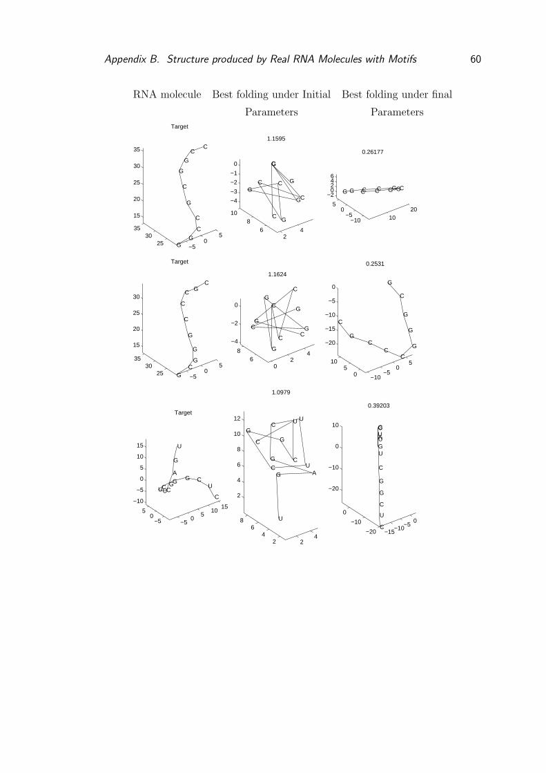
Appendix B. Structure produced by Real RNA Molecules with Motifs 60
RNA molecule Best folding under Initial Best folding under final
Parameters Parameters
−50
525
3035
15
20
25
30
35 C
C
C
C
G
G
G
C
Target
G
G2
468
10
−4
−3
−2
−1
0
CG
G
G
C
1.1595
C
GC
CG
1020
−10−5
05
−20246
CGGGCC
0.26177
CCGG
−50
525
3035
15
20
25
30
CG
G
G
C
G
C
C
C
Target
G
02
46
8
−4
−2
0
GC
G
C
C
1.1624
G
CG
GC
−10−5
05
05
10
−20
−15
−10
−5
0
G
G
G
C
C
G
C
0.2531
CG
C
−50
510
15
−50
5
−10
−5
0
5
10
15
C
UCG
Target
U
G
AGG
CUCU
24
24
68
2
4
6
8
10
12
AU
U
C
U
1.0979
G
U
G
C
C
G
C
G
−15−10
−50
−20
−10
0
−20
−10
0
10
C
U
C
G
G
0.39203
C
U
UG
C
A
GU

Appendix B. Structure produced by Real RNA Molecules with Motifs 61
RNA molecule Best folding under Initial Best folding under final
Parameters Parameters
1520
25−5
05
−30
−25
−20
−15
−10
−5
0
5
10
15
20
A
G
G
G
C
A
C
A
A
Target
G
U
U
UG
CC
C
CC
24
68
46
8
−12
−10
−8
−6
−4
−2
0
2
4
A
C
G
U
CGCCG
A
UA
U
0.94021
GC
C
C
G
A
−30−20
−100
010
20
−505
AA
G
UG
C
C
CC
C
U
0.45836
U
A
G
CGACG
510
1520
2530
35
5
10
15
20
25U
C
G
C
GC
Target
UU
G
C
G
A
24
68
10
12345
0
2
4
6
8
UU
A
1.1172
U
CGC
G
G
C
CG
510
150
510
−10
−5
0
5
10
CGU
U
G
A
C
0.43994
U
GG
CC
Table B.1: Structure produced with motifs and learnt
parameters. Number above each graph indicates the er-
ror

Bibliography
[1] Kim T. Simons Ingo Ruczinski Charles Kooperberg Brian A. Fox Chris
Bystroff and David Baker Improved Recognition of Native-Like Protein
Structures Using a Combination of Sequence-Dependent and Sequence-
Independent Features of Proteins PROTEINS: Structure, Function, and Ge-
netics 34:82-95 (1999)
[2] Kim T. Simons, Charles Kooperberg, Enoch Huang and David Baker As-
sembly of Protein Tertiary Structure from Framents with Similar Local Se-
quences using Simulated Annealing and Bayesian Scoring Functions J. Mol.
Biol. (1997) 268, 209-225
[3] Karen F.Han Christopher Bystroff and Davd Baker Three-dimensional struc-
tures and contexts associated with recurrent amino acid sequence patterns
Protein Science (1997) 6 1587-1590, Cambridge University Press
[4] Christopher Bystroff An Alternative Derivation of the Equations of Motion
in Torsion Space for a Branched Linear Chain Protein Engineering vol.14
no.11 pp.825-828, 2001
[5] Carol A. Rohl and David Baker De Novo Determination of Protein Backbone
Structure from Residual Dipolar Couplings Using Rosetta J. Am. Chem. Soc.
Vol 124, No 11, pp.2723-2729, 2002
[6] R. E. Shapire. The boosting approach to machine learning: An overview
MSRI Workshop on Nonlinear Estimation and Classification, 2002.
http://www.cs.princeton.edu/ schapire/papers/msri.ps.gz
62

Bibliography 63
[7] Micheal Zuker On Finding All Suboptimal Foldings of an RNA Molecule
Science, New Series, Volume 244, Issue 4900 (Apr 7, 1989), 48-52
[8] Rune B. Lyngs, Michael Zuker and Christian N. S. Pedersen An Improved
Algorithm for RNA Secondary Structure Prediction BRICS RS-99-15 May
1999
[9] A. Zuker, B. Mathews and C. Turner Algorithms and Thermodynamics for
RNA Secondary Structure Prediction: A Practical Guide MFold manual
http://www.bioinfo.rpi.edu/ zukerm/export/mfold-3.0-manual.pdf
[10] DNA, RNA, PNA; stepping backwards in time http://exobio.ucsd.edu/
Space_Sciences/rna-dna.htm A summary of an unavailable in time paper
Gerald Joyce Nature, Vol. 338 (1989) pp. 217-224
[11] Ulrik Kjems Parallel Matlab http://bond.imm.dtu.dk/plab/about.html
[12] Ian Nabney and Christopher M. Bishop Netlab neural network software
http://www.ncrg.aston.ac.uk/netlab/index.html
[13] F. Eckstein RNA and DNA as Catalysts Unpublished, available at
http://www.mpibpc.gwdg.de/inform/MpiNews/cientif/jahrg5/9.99/scta.html
[14] David J.C. MacKay Information Theory, Inference and Learning Algorithms
360-381
[15] Chen Yanover and Yair Weiss Approximate Inference
and Protein Folding NIPS*2002 Paper AP08 (2002)
http://www.cs.huji.ac.il/ cheny/sidechain/sc.pdf
[16] H. M. Berman, W. K. Olson, D. L. Beveridge, J. Westbrook, A. Gel-
bin, T. Demeny, S.-H. Hsieh, A. R. Srinivasan, and B. Schneider. The
Nucleic Acid Database: A Comprehensive Relational Database of Three-
Dimensional Structures of Nucleic Acids. Biophys. J., 63, 751-759. (1992)
http://beta-ndb.rutgers.edu/
[17] John W. Eaton Octave http://www.octave.org/