data-driven kernels for support vector machines · data-driven kernels for support vector machines...

Data-driven Kernels for SupportVector Machines

by

Xin Yao

A research paperpresented to the University of Waterloo

in partial fulfillment of therequirement for the degree of

Master of Mathematicsin

Computational Mathematics

Supervisor: Prof. Yuying Li

Waterloo, Ontario, Canada, 2013

c© Xin Yao 2013

I hereby declare that I am the sole author of this report. This is a true copy of the report,including any required final revisions, as accepted by my examiners.

I understand that my report may be made electronically available to the public.

ii

Abstract

Kernel functions can map data points to a non-linear feature space implicitly, andthus significantly enhance the effectiveness of some linear models like SVMs. However, incurrent literature, there is a lack of a proper kernel that can deal with categorical featuresnaturally.

In this paper, we present a novel kernel for SVM classification based on data-drivensimilarity measures to compute the similarity between two samples. It then followed bythe ensemble selection method to combine all similarity measures. Our kernels can makefull use of information from both labeled and unlabeled data, which leads to a semi-supervised approach. Experiment results show that our approaches largely improve theperformance of SVMs on all metrics we used. Especially, in the unbalanced class case,keeping other performance measures on an excellent level, two methods can enhance theprediction accuracy on the minority class significantly.

iii

Acknowledgements

I would like to thank all the people who have made this work possible.

iv

Table of Contents

List of Tables vii

List of Figures viii

1 Introduction 1

2 Support Vector Machines 3

2.1 Support Vector Machine Formulations . . . . . . . . . . . . . . . . . . . . 3

2.1.1 Hard-Margin Support Vector Machines . . . . . . . . . . . . . . . . 3

2.1.2 Soft-Margin Support Vector Machines . . . . . . . . . . . . . . . . . 7

2.2 Kernel Trick . . . . . . . . . . . . . . . . . . . . . . . . . . . . . . . . . . . 11

3 Methodology 14

3.1 Similarity Measures . . . . . . . . . . . . . . . . . . . . . . . . . . . . . . . 14

3.2 Ensemble Selection Method . . . . . . . . . . . . . . . . . . . . . . . . . . 17

3.3 Approach . . . . . . . . . . . . . . . . . . . . . . . . . . . . . . . . . . . . 20

4 Numerical Results 21

4.1 Data Preprocessing and Cleaning . . . . . . . . . . . . . . . . . . . . . . . 22

4.2 Feature Selection . . . . . . . . . . . . . . . . . . . . . . . . . . . . . . . . 23

4.3 Results of SVMs with the RBF kernel . . . . . . . . . . . . . . . . . . . . . 24

4.4 Results of SVMs with the Lin Similarity Measure . . . . . . . . . . . . . . 25

v

4.5 Results of the Ensemble Selection Method . . . . . . . . . . . . . . . . . . 27

4.6 Comparison of Three Methods . . . . . . . . . . . . . . . . . . . . . . . . . 29

5 Conclusion 32

References 32

vi

List of Tables

3.1 Similarity Measure for Categorical Features . . . . . . . . . . . . . . . . . 16

4.1 Frequency of labels of churn, appetency and up-selling . . . . . . . . . . . 22

4.2 Top 5 feature importance scorse from random forests . . . . . . . . . . . . 24

4.3 Performance of RBF kernel SVMs. . . . . . . . . . . . . . . . . . . . . . . 26

4.4 Performance of SVMs with Lin similarity measure. . . . . . . . . . . . . . 27

4.5 Performance of the Ensemble Selection Method. . . . . . . . . . . . . . . . 29

4.6 Best performance of each method . . . . . . . . . . . . . . . . . . . . . . . 31

vii

List of Figures

2.1 Two separating hyperplane with different margins. . . . . . . . . . . . . . . 5

2.2 Inseparable case in a two-dimensional space . . . . . . . . . . . . . . . . . 8

2.3 The idea of non-linear SVM. . . . . . . . . . . . . . . . . . . . . . . . . . . 12

4.1 ROC and Precision-Recall Curves of SVMs with Lin Similarity Measure . . 25

4.2 ROC and Precision-Recall Curves of Ensemble Selection Method . . . . . . 28

4.3 ROC and Precision-Recall Curves of the Ensemble Selection Method . . . 30

viii

Chapter 1

Introduction

Over the past decade, Support Vector Machine (SVM) has become a significant tool forsolving classification problems in statistical learning and data mining. A natural wayof solving classification problems is seeking a hyperplane to separate the classes. Withperfectly separable classes, there exists infinite possible separating hyperplanes. SVM isbased on the principle of finding the “best” hyperplane which is the one that is farthestaway from the classes. This principle is called maximal margin principle. The hyperplanecan be obtained by solving a convex quadratic optimization problem. However, in thereal world, most problems are not perfectly separable. Hence, a nonlinear transformationneeds to be done to separate classes effectively in another high dimensional space. Throughkernel functions, we can map the input features to this nonlinear feature space, withoutcomputing the mapping explicitly. In this space, SVM finds a linear separating hyperplanewith the maximal margin. An important advantage of the kernel-based SVM is that themapping can be done using the “kernel trick”. The trick computes this transformationimplicitly and efficiently. Another advantage is that using `2 penalty, SVM successfullystabilizes the solution and overcomes over-fitting especially in high-dimensional problems.Consequently, choosing a proper kernel function is central for the effectiveness of a SVMmodel.

In previous studies, many kernel functions have been proposed to capture properties ofdata. Radial basis function (RBF) kernels are the most common choice and has been usedextensively in the machine learning field. Using RBF kernels means choosing radial basisfunction networks [9] as the prior hypothesis. Diffusion kernels [17] are widely used toanalyze the network data. They can be used to unfold correlated structures between nodesof networks in an Euclidean space. As natural language text mining becomes increasingly

1

important, by assigning to each pair of elements (strings) an “inner product” in a featurespace, string kernels [19] are employed especially for text classification tasks.

Although many kernel functions have been developed for different types of data, thereis a lack of a proper kernel to deal with categorical data naturally. Categorical data isone kind of data that each value can take one of a limited and usually fixed number ofpossible values. Categorical data widely exists in many data mining problems, for exam-ple, customer behavior data mining tasks, when predicting customer loyalty or managingcustomer relationship in modern marketing strategies. Problems, containing categoricalfeatures with many different possible values, a large number of missing values, and unbal-anced class proportions, attract more and more attention in data mining field these days[2, 13].

In this research project, we explore a novel kernel based on data-driven similaritymeasures which are used to compute the similarity between categorical data instances. Ourmotivation comes from two facts: kernel functions can be viewed as a similarity measurebetween two input vectors, and using information of both labeled and unlabeled sets maysignificantly improve performance. The latter approach usually is called semi-supervisedlearning in the literature. Moreover, in order to combine different similarity measures,the ensemble selection [7] approach is used to optimize the overall performance of diversesimilarity kernel-based SVMs. Under the SVM framework, we compare the performanceof our kernel with the standard RBF kernel and other leading classification models on acustomer loyalty prediction problem.

The rest of the paper is organized as follows: Chapter 2 provides some backgroundknowledge on SVM and kernel trick. Chapter 3 describes our novel kernel with similaritymeasures and the ensemble selection method. Chapter 4 compares performance of ourapproach with common used RBF kernels on customer loyalty data. Chapter 5 summarizesthe paper with further discussion.

2

Chapter 2

Support Vector Machines

In this chapter, we discuss SVM for the two-class classification problem. Firstly, we discusshard-margin SVMs, which assumes that the training data points are linearly separable inthe input space. Although it cannot be used in many real world situations, it is the easiestmodel to understand and it forms the foundation of more complex SVMs. Secondly, weextend hard-margin SVMs to the soft-margin SVMs which is for the case when training datapoints are not linearly separable. Then we introduce the “kernel trick” to do classificationin the nonlinear feature space to enhance separability.

2.1 Support Vector Machine Formulations

2.1.1 Hard-Margin Support Vector Machines

The discussion follows the formulation of [22] and [24]. In a two-class classification problem,we have M m-dimensional training data points xi (i = 1, . . . ,M) and the associated classlabels be yi ∈ {−1, +1}. SVMs seek an optimal hyperplane to separate the two classes.

A hyperplane in Rm can be described with a linear equation with the following formfor some nonzero vector w ∈ Rm and b ∈ R

w>x + b = 0. (2.1)

The hyperplane

yi(w>xi + b

)≥ c, for i = 1, . . . ,M, and c > 0, (2.2)

3

forms a separating hyperplane that separates {xi : yi = 1} and {xi : yi = −1}.

A hyperplane can be arbitrarily rescaled, for example,

w>x + b = 0 is equaivalent to s(w>x + b

)= 0, ∀s 6= 0. (2.3)

In particular, the hyperplane (2.2) can be reparameterized as

yi(w>xi + b

)≥ 1, for i = 1, . . . ,M. (2.4)

A separating hyperplane satisfying condition (2.4) is called a canonical separating hy-perplane.

This way, we can have a decision function

w>xi + b

{> 0 for yi = 1,

< 0 for yi = −1.(2.5)

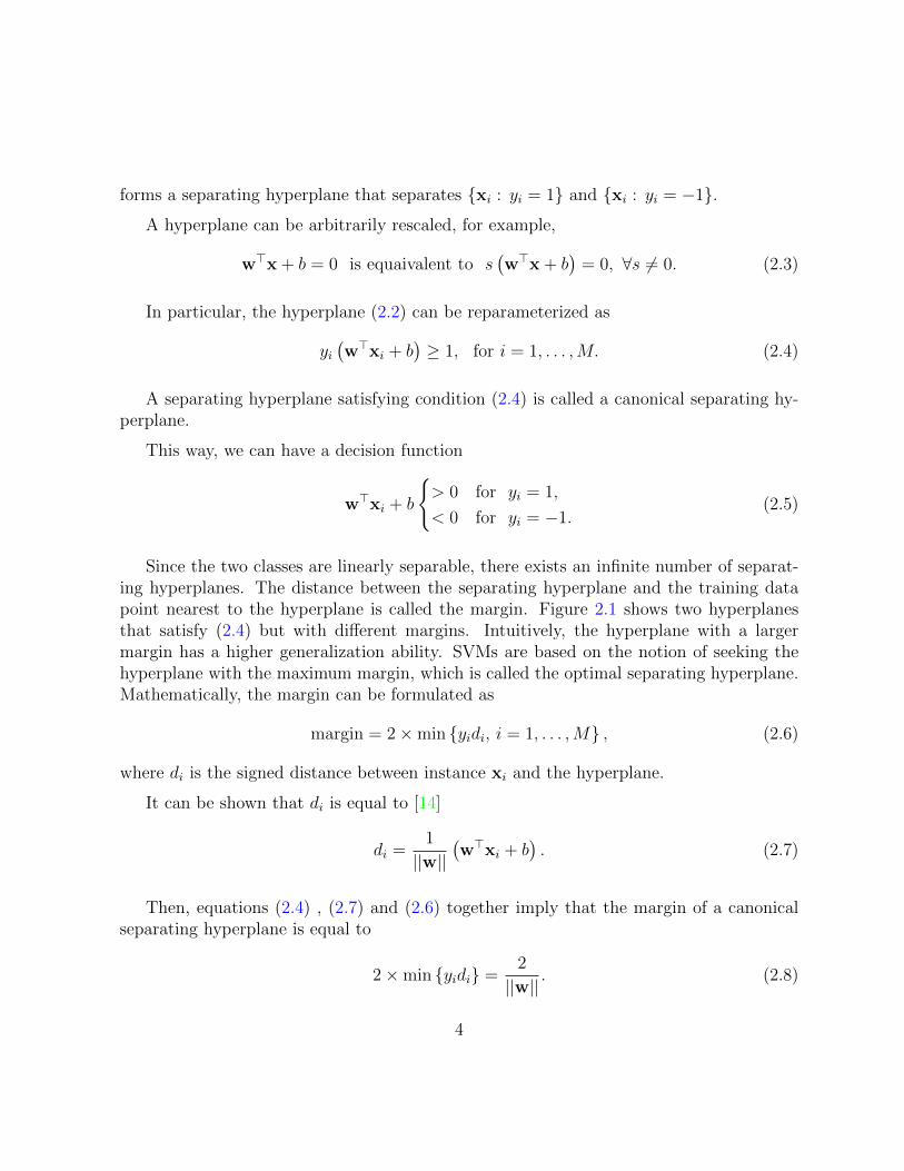
Since the two classes are linearly separable, there exists an infinite number of separat-ing hyperplanes. The distance between the separating hyperplane and the training datapoint nearest to the hyperplane is called the margin. Figure 2.1 shows two hyperplanesthat satisfy (2.4) but with different margins. Intuitively, the hyperplane with a largermargin has a higher generalization ability. SVMs are based on the notion of seeking thehyperplane with the maximum margin, which is called the optimal separating hyperplane.Mathematically, the margin can be formulated as

margin = 2×min {yidi, i = 1, . . . ,M} , (2.6)

where di is the signed distance between instance xi and the hyperplane.

It can be shown that di is equal to [14]

di =1

||w||(w>xi + b

). (2.7)

Then, equations (2.4) , (2.7) and (2.6) together imply that the margin of a canonicalseparating hyperplane is equal to

2×min {yidi} =2

||w||. (2.8)

4

Margin (Better)

Margin (Worse)

Support Vector

Support Vector

Figure 2.1: Two separating hyperplane with different margins. Adapted from [24]

Therefore, the optimal separating hyperplane can be obtained by solving the followingoptimization problem for w and b:

min1

2||w||2 (2.9)

s.t. yi(w>xi + b

)≥ 1, for i = 1, . . . ,M. (2.10)

Problem (2.9) is a convex quadratic programming problem. The assumption of linearseparability means that there exist w and b that satisfy (2.10). Because the optimizationproblem has a convex quadratic objective function with linear inequality constraints, evenif the solutions are not unique, a local minimizer is always a global minimizer. This is oneof the advantages of support vector machines.

This constrained optimization problem can be solved by introducing Lagrange multi-pliers αi ≥ 0 and a Lagrangian

L(w, b, α) =1

2w>w −

M∑i=1

αi(yi(w>xi + b

)− 1), (2.11)

5

where α = (α1, . . . , αM)>. The Lagrangian L has to be minimized with respect to theprimal variables w and b, and maximized with respect to the dual variables αi, i.e. asaddle point has to be found.

The solution satisfies the following Karush-Kuhn-Tucker (KKT) conditions:

∂

∂wL(w, b, α) = 0, (2.12)

∂

∂bL (w, b, α) = 0, (2.13)

yi(w>xi + b

)≥ 1 for i = 1, . . . ,M, (2.14)

αi(yi(w>xi + b

)− 1)

= 0 for i = 1, . . . ,M, (2.15)

αi ≥ 0 for i = 1, . . . ,M. (2.16)

Specifically, equations (2.15) which link inequality constraints and their associated La-grange multipliers are called KKT complementarity conditions.

Equation (2.15) implies that either αi = 0, or αi 6= 0 and yi(w>xi + b

)= 1, must be

satisfied. The training data points, whose αi 6= 0, are called Support Vectors. Supportvectors lie on the margin (Figure 2.1). All remaining samples do not show up in the finaldecision function: their constraints are inactive at the solution. This nicely captures theintuition of the problem that the hyperplane is determined by the points closest to it.

Using (2.11), (2.12) and (2.13) are reduced to

w =M∑i=1

αiyixi (2.17)

andM∑i=1

αiyi = 0. (2.18)

By substituting (2.17) and (2.18) into (2.11), one eliminates the primal variables andarrives at the dual problem:

maxM∑i=1

αi −1

2

M∑i, j=1

αiαjyiyjx>i xj (2.19)

s.t.M∑i=1

αiyi = 0, and αi ≥ 0, i = 1, . . . ,M. (2.20)

6

The formulated support vector machine is called the hard-margin support vector ma-chine. Because

1

2

M∑i, j=1

αiαjyiyjx>i xj =

1

2

(M∑i=1

αiyixi

)>( M∑i=1

αiyixi

)≥ 0, ∀αi (2.21)

maximizing (2.19) under the constraints (2.20) is a concave quadratic programming prob-lem. If a solution exists, specially, if the classification problem is linearly separable, theglobal optimal solution αi (i = 1, . . . ,M) exists. For convex quadratic programming, thevalues of the primal and dual objective functions coincide at the optimal solutions if theyexist, which is called zero duality gap.

Data that are associated with αi 6= 0 are support vectors for class with 1 or −1. Thenfrom (2.5) and (2.17) the decision function is given by

D(x) =∑i∈S

αiyix>i x + b, (2.22)

where S is the set of support vectors, and from the KKT conditions, b is given by

b = yi −w>xi, for i ∈ S. (2.23)

Then unknown data sample x is classified into{y = +1 if D(x) > 0,

y = −1 if D(x) < 0.(2.24)

If D(x) = 0, x is on the boundary and thus is unclassifiable. When the training data areseparable, the region {x | − 1 < D(x) < 1} is the generalization region.

2.1.2 Soft-Margin Support Vector Machines

In the hard-margin SVM, we assume that the training data are linearly separable. But inpractice, a separating hyperplane may not exist, e.g. if a high noise level causes a largeoverlap of the classes. As a result, there is no feasible solution to the hard-margin SVM sothat it becomes unsolvable. Here we extend the hard-margin SVM so that it is applicableto an inseparable case.

To allow for the possibility of data points violating (2.10), we introduce slack variables

ξi ≥ 0, i = 1, . . . ,M (2.25)

7

ξ𝑗

ξ𝑖

Figure 2.2: Inseparable case in a two-dimensional space

along with relaxed constraints

yi(w>xi + b

)≥ 1− ξi, i = 1, . . . ,M. (2.26)

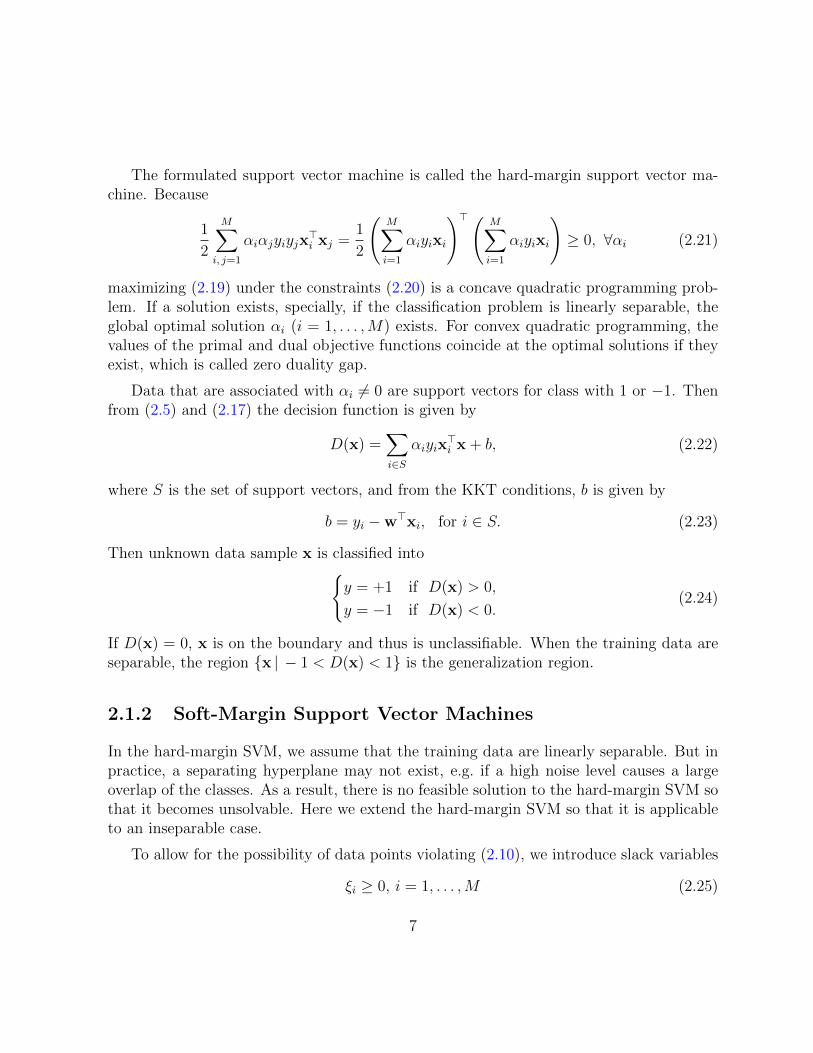
With the slack variable ξi, feasible solutions always exist. For the training data xi, if0 < ξi < 1 (ξi in Figure 2.2), the data does not have the maximum margin but are stillcorrectly classified. But if ξi ≥ 1 (ξj in Figure 2.2) the data is misclassified by the optimalhyperplane.

In order to find the hyperplane which generalizes well, both the margin and the numberof training errors need to be controlled. Thus, we consider the following optimizationproblem:

min1

2||w||2 + C

M∑i=1

ξi (2.27)

s.t. yi(w>xi + b

)≥ 1− ξi, i = 1, . . . ,M, (2.28)

ξi ≥ 0, i = 1, . . . ,M.

8

where C is the margin parameter that determines the trade-off between the maximizationof the margin and the minimization of the classification error. A larger C penalizes moreon classification errors, consequently, leading to a lower classification error but a smallermargin. As C decreases, we will have a larger margin but a higher classification error.Because of slack variables, we call the SVM the soft-margin-SVM.

Similar to the linearly separable case, introducing the nonnegative Lagrange multipliersαi and βi, we obtain

L (w, b, ξ, α, β) =1

2||w||2 + C

M∑i=1

ξi −M∑i=1

βiξi

−M∑i=1

αi(yi(w>xi + b

)− 1 + ξi

), (2.29)

where α = (α1, . . . , αM)>, ξ = (ξ1, . . . , ξM)>, and β = (β1, . . . , βM)> .

For the optimal solution, the following KKT conditions are satisfied:

∂L (w, b, ξ, α, β)

∂w= 0, (2.30)

∂L (w, b, ξ, α, β)

∂b= 0, (2.31)

∂L (w, b, ξ, α, β)

∂ξ= 0. (2.32)

αi(yi(w>xi + b

)− 1 + ξi

)= 0 for i = 1, . . . ,M, (2.33)

yi(w>xi + b

)≥ 1− ξi for i = 1, . . . ,M, (2.34)

βiξi = 0 for i = 1, . . . ,M, (2.35)

αi ≥ 0, βi ≥ 0, ξi ≥ 0 for i = 1, . . . ,M. (2.36)

Using (2.29), we reduce (2.30) to (2.32), respectively, to

w =M∑i=1

αiyixi, (2.37)

M∑i=1

αiyi = 0, (2.38)

αi + βi = C for i = 1, . . . ,M. (2.39)

9

Thus substituting (2.37) to (2.39) into (2.29), we obtain the following dual problem:

minM∑i=1

αi −1

2

M∑i, j=1

αiαjyiyjx>i xj (2.40)

s.t.M∑i=1

αiyi = 0 for i = 1, . . . ,M, (2.41)

C ≥ αi ≥ 0 for i = 1, . . . ,M. (2.42)

The only difference between soft-margin SVMs and hard-margin SVMs is the upper boundC on the Lagrange multiplies αi. The inequality constraints in (2.42) are called boxconstraints.

Especially, (2.33) and (2.35) are called KKT complementarity conditions. From these,there are three cases for αi:

1. αi = 0. Then ξi = 0. Thus, xi is correctly classified.

2. 0 < αi < C. Then yi(w>xi + b

)−1+ξi = 0 and ξi = 0. Therefore, yi

(w>xi + b

)= 1

and xi is a support vector. Especially, we call the support vector with C > αi > 0an unbounded support vector.

3. αi = C. Then yi(w>xi + b

)− 1 + ξi = 0 and ξi ≥ 0. Thus xi is a support vector.

We call the support vector with αi = C a bounded support vector. If 0 ≤ ξi ≤ 1, xiis correctly classified, and if ξi ≥ 1, xi is misclassified.

The decision function is the same as that of the hard-margin SVM and is given by

D(x) =∑i∈S

αiyix>i x + b, (2.43)

where S is the set of support vectors.

Then unknown data sample is classified into{y = +1 if D(x) > 0,

y = −1 if D(x) < 0.(2.44)

If D(x) = 0, x is on the boundary and thus is unclassifiable. When there is no boundedsupport vector, the region {x | − 1 < D(x) < 1} is the generalization region, which is thesame as the hard-margin SVM.

10

2.2 Kernel Trick

SVMs construct an optimal hyperplane with the largest margin in the input space. Thelimited classification power of linear models was highlighted in the 1960s by Minsky andPapert [20]. Using a linear model means having a hypothesis that data points are linearlyor almost linearly separable. However, many real-world applications require more complexhypotheses than that of linear models. On the other hand, the optimal hyperplane isa linear combination of the input features. But labels usually cannot be separated bya simple linear combination of the input features. Consequently, more complex featuremappings are required to be exploited.

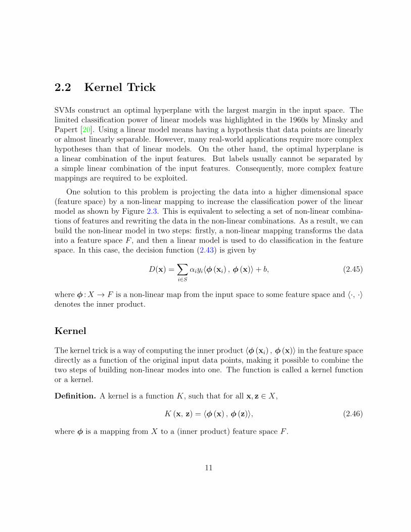
One solution to this problem is projecting the data into a higher dimensional space(feature space) by a non-linear mapping to increase the classification power of the linearmodel as shown by Figure 2.3. This is equivalent to selecting a set of non-linear combina-tions of features and rewriting the data in the non-linear combinations. As a result, we canbuild the non-linear model in two steps: firstly, a non-linear mapping transforms the datainto a feature space F , and then a linear model is used to do classification in the featurespace. In this case, the decision function (2.43) is given by

D(x) =∑i∈S

αiyi〈φ (xi) , φ (x)〉+ b, (2.45)

where φ :X → F is a non-linear map from the input space to some feature space and 〈·, ·〉denotes the inner product.

Kernel

The kernel trick is a way of computing the inner product 〈φ (xi) , φ (x)〉 in the feature spacedirectly as a function of the original input data points, making it possible to combine thetwo steps of building non-linear modes into one. The function is called a kernel functionor a kernel.

Definition. A kernel is a function K, such that for all x, z ∈ X,

K (x, z) = 〈φ (x) , φ (z)〉, (2.46)

where φ is a mapping from X to a (inner product) feature space F .

11

O

O

O

O

X

X X

X

Φ(O)

Φ(O)

Φ(O)

Φ(O)

Φ(X)

Φ(X)

Φ(X)

Φ(X)

X F

Φ

Input Space Feature Space

Figure 2.3: The idea of non-linear SVM: map the data points into a higher dimensionalspace via function Φ, then construct a hyperplane in feature space. This results in anonlinear decision boundary in the input space. Adapted from [21].

Example. Radial basis function (RBF) kernel can be written as

K(x, z) = e−γ||x−z||2

, (2.47)

where γ is known as the width scalar. In [23], Steinwart et al. argue that RBF kernel mapsdata points into a infinite-dimensional space. But when computing the inner product inthis infinite-dimensional space by the RBF kernel, we don’t need to know the informationof the corresponding feature mapping φ.

Using the kernel function, the decision function (2.43) can be rewritten as

D(x) =∑i∈S

αiyiK (xi, x) + b. (2.48)

Functions of Kernel

One important fact of the kernelized dual form (equation (2.48)) is that the dimension offeature space does not effect the computation. Because kernel functions make it possible

12

to map the data implicitly into a feature and train the linear model in that space, one doesnot represent the feature vectors explicitly. The number of operations required to computethe inner product by evaluating kernel functions is not proportional to the number ofdimensions of the feature space. For example, although the RBF kernel maps data pointsinto a infinite-dimensional space, the number of operations required to evaluate the kernelfunction is not infinity. In this way, without knowing the underlying feature mapping, wecan still compute inner product in the feature space by kernel functions and be able tolearn the linear model in the feature space.

In addition to being regarded as a shortcut of computing inner product in the featurespace, kernels can also be viewed as a function to measure similarity between two vectors.

Provided that two vectors x and x′ are normalized to length 1, the inner product of twovectors can be interpreted as computing the cosine of the angle between these two vectors.The resulting cosine ranges from −1 to 1. A value of −1 means that two vectors are exactlyopposite and 1 means that they are exactly the same. The zero value usually indicatesindependence of the two vectors and in-between values indicates intermediate similarity.Thus, the inner product of two normalized vectors can be viewed as a similarity of thesetwo vectors.

Embedding data into a feature space provides the freedom to choose the mapping φ.The inner product (similarity) is not restricted to the input space, but also can be usedin the feature space. Kernel functions offer the possibility of computing the mapping andinner product implicitly. At the same time, kernel functions can be viewed as a similarityof two vectors. Moreover, it enable us to design a large variety of similarity measuresinstead of figuring out an interpretable geometric space.

13

Chapter 3

Methodology

Now, we discuss two methodologies to improve the performance of SVMs on categoricaldata. Firstly, different data-driven similarity measures are used to capture the relationshipbetween two samples, and used as the kernel matrix in SVMs. Unlike standard kernelslike the RBF kernel that does not depend on test data, these data-driven similarities canuse the information in both the training and test data. As a result, they can extract moreinformation from the underlying distribution of the dataset. Then, in order to combinebenefits of each similarity measure, an ensemble selection method is used to construct anensemble from a library of SVM models with different similarity measures. The ensem-ble selection method allows models to be optimized to different performance evaluationmethods.

3.1 Similarity Measures

The use of kernels is an attractive computational shortcut. Although it is possible to createa feature space and work out an inner product in that space, in practice, the approachtaken is to define a kernel function directly. Consequently, both the computation of innerproduct and design of a feature space can be avoided.

There are several ways to design a kernel by defining the kernel function directly. In[21], Schlkopf et el. show that one can make a kernel by taking linear combination ofother kernels. Another way of making a kernel comes from designing an inner product.However, all these methods share the same problem that the information from the test datais ignored. As a consequence, if the training data is biased, i.e. training samples cannot

14

represent the population well, for example, when labels are unbalanced or training set issmall, the prediction error can be large.

To solve this problem, we can design a new kind of kernels which can make full useof information in the whole dataset. Since a kernel function can be viewed as a similaritybetween two vectors, a more intuitive way of designing a kernel may be using a data-driven similarity measure. Such data-driven similarity measures take into account thefrequency distribution of different feature values in a dataset to define a similarity measurebetween two categorical feature values. As a result, even though the training set may beunbalanced or small, when computing the frequency, these data-driven similarity basedkernels can reduce the bias by involving information in both training and test data. In theliterature, the notion of using information of both labeled (training) and unlabeled (test)data is called semi-supervised learning.

The following discussion follows the formulation of [3]. For the sake of notation, considera categorical dataset D containing N samples and d features. Define Ak as the kth featureand it takes nk values in the dataset. Then we can define the following notation:

• fk(x): The number of times feature Ak takes the value x in the dataset D.

• pk(x): The sample probability of feature Ak to take the value x in the dataset D.The sample probability is given by

pk(x) =fk(x)

N. (3.1)

• p2k(x): Another probability estimation [12] of feature Ak to take the value x in thegiven dataset D is given by

p2k(x) =fk(x) (fk(x)− 1)

N(N − 1). (3.2)

Usually, the similarity measure assigns a similarity value between two samples X and Ybelonging to the dataset D as follows:

S(X, Y ) =d∑

k=1

wkSk(Xk, Yk), (3.3)

where Sk(Xk, Yk) is the feature similarity between two values for one categorical featureAk and Xk and Yk are the kth values of sample X and Y respectively. The quantity wkdenotes the weight assigned to the feature Ak.

Table 3.1 summarizes the mathematical formulas for the similarities used in this paper.Adapted from Table 2 in [3], Table 3.1 only lists similarity measures used in this work.

15

Measure Sk (Xk, Yk) wk, k = 1, . . . , d

Overlap =

{1 if Xk = Yk

0 otherwise1d

IOF =

{1 if Xk = Yk

11+log fk(Xk) log fk(Yk)

otherwise1d

OF =

{1 if Xk = Yk

11+log N

fk(Xk)log N

fk(Yk)

otherwise1d

Lin =

{2 log pk(Xk) if Xk = Yk

2 log(pk(Xk) + pk(Yk)) otherwise1∑d

i=1 log pi(Xi)+log pi(Yi)

Goodall1 =

1−∑p2k(q)q∈Q

if Xk = Yk

0 otherwise

1d

Goodall2 =

1−∑p2k(q)q∈Q

if Xk = Yk

0 otherwise

1d

Goodall3 =

{1− p2k(Xk) if Xk = Yk

0 otherwise1d

Goodall4 =

{p2k(Xk) if Xk = Yk

0 otherwise1d

Table 3.1: Similarity Measure for Categorical Features. For mea-sure Goodall1, {Q ⊆ Ak : ∀q ∈ Q, pk(q) ≤ pk(Xk)} . For measure Goodall2,{Q ⊆ Ak : ∀q ∈ Q, pk(q) ≥ pk(Xk)} . Adapted from [3].

16

Characteristics of similarity measures

According to the quantities being used, similarity measures listed in Table 3.1 may beclassified into four groups.

Overlap is the simplest measure listed in the table. It is developed based on the ideaof computing proportion of matching features in two samples. Sk is assigned to a value of1 if the kth feature of two samples are the same and a value of 0 if they are different. Inaddition, it equally weights matches and mismatches.

Originally used for the information retrieval in documents, OF and IOF involve thefrequency of values in a feature. The main difference of these two measures is giving differ-ent similarities to mismatches. The IOF measure assigns lower similarity to mismatcheson more frequent values and higher similarity to mismatches on less frequent values, whilethe IF measure assigns the opposite weights.

Lin is a special measure because it not only uses the probability estimation pk, butalso follows the information-theoretic framework proposed by Lin in [18]. In terms ofweights, Lin measure gives more weights to matches on frequent values and low weightsto mismatches on infrequent values. Moreover, results in [18] show that Lin measure hasan excellent performance on measuring similarity of categorical samples. As a result, inthe experiments, the Lin measure will be used as the example of data-driven similaritymeasures.

Because of using another probability estimation p2k(x), Goodall1, Goodall2, Goodall3,and Goodall4 are clustered into one group. The first difference among these four measuresis that Goodall1 and Goodall2 use the cumulative probability of other values in the featureeither more or less frequent than than the current showing up one. Regardless of othervalues, Goodall3 and Goodall4 just involve the probability of the common values that twosamples share. Secondly, in terms of weighting, Goodall1 and Goodall3 assigns highersimilarity if the matching values are infrequent. While Goodall2 and Goodall4 assign theopposite similarity.

3.2 Ensemble Selection Method

An ensemble constructs a collection of models (base models) whose predictions are com-bined by weighted average or majority vote. Mathematically, it can be formulated as

F (y|x) =∑m∈M

wmfm(y|x), (3.4)

17

where M is the index set of base models which are chosen, wm are the weights for thecorresponding base models fm and F is the final ensemble. A large number of research hasshown that compared with the single model, ensemble methods can increases performancesignificantly (e.g. [5, 6, 11]). However, these usual ensemble methods either simply averageall the base models without any selection, or collect a single kind of base model like treemodel.

Ensemble selection [7] was proposed as an approach of building ensembles by selectingfrom large collection of diverse models. Compared with other ensemble methods, theensemble selection method benefits from the ability of using many more base models andincludes a selection process. Especially, ensemble selection’s ability to optimize to anyperformance metric is an attractive capability of the method that is useful in domainswhich use non-traditional performance evaluation measures like AUC and AP [10].

The ensemble selection method as shown in Algorithm 3.1 is a two-step procedure.Before the procedure, the whole dataset is equally divided into three subsets. One subsetis used for training base models; another one is for validation and the other one is fortesting the ensemble performance. The two-step procedure begins by training modelsusing as many type of models and tuning parameters as can be applied to the problem.Little attempt is made to optimize the performance of single models in the first step; allmodels no matter what their performance, are candidates in the model library for furtherselection. It is then followed by selecting a subset of models from the model library thatyield the best performance on the performance metric. The selecting step can be doneby using a forward stepwise model selection, i.e., at each step selecting the base model inthe library that maximizes the performance of the ensemble if added. The performanceof adding a potential model to the ensemble is evaluated by combining the prediction ofselected base models and the potential model on the validation set.

Preventing overfitting

The forward stepwise selection may encounter a problem that the ensemble performs muchbetter on the training set than on the test set, namely overfitting, in the selection procedure.The reason of overfitting in the ensemble selection is that by greedily selecting the best basemodel at each step, the ensemble yields a extremely good performance on the validationset. Under this circumstance, the selection stops when the ensemble is small.

Caruana et al. suggest the sorted ensemble initialization approach [7] to address theoverfitting problem. Specifically, instead of starting with an empty ensemble, sort themodels in the library by their performance on the validation set, and put the best N

18

Algorithm 3.1 Ensemble Selection Algorithm

1. Start with the empty ensemble.

2. Repeat, until no model can improve the ensemble’s performance:

(a) Choose the model i in the library that maximizes the ensemble performance tothe metric after being added.

(b) Set

M ← M ∪ i,

F (y|x) =∑m∈M

1

|M |fm(y|x).

Break

3. Output an ensemble selection model

F (y|x) =∑m∈M

1

|M |fm(y|x). (3.5)

19

models in the ensemble. N is chosen by the size of model library. As a result, the ensemblewill not contain only those models that overfit the training set.

3.3 Approach

Based on the discussion of similarity measures and ensemble selection method, we proposetwo approaches to improve the performance SVM model on the categorical data.

Firstly, in order to deal with categorical data naturally, we use the data-driven similaritymeasures listed in Table 3.1 as the kernel function in SVM models. Since data-drivensimilarity measures use information from both training and test set, this approach cangive a better estimation of the similarity between samples.

Secondly, in order to combine benefits of those similarity measures, we use ensembleselection technique to build up an ensemble of SVM models with different similarity mea-sures. In doing so, we take advantage of data-driven similarity measures and the ensemblemethod.

20

Chapter 4

Numerical Results

In this chapter, we present numerical results of the two approaches discussed in Chapter 3.These two methods are applied to the dataset from KDD Cup 20091, provided by a FrenchTelecom company. The task of the competition is to predict the customer behavior from thecustomer data. The competition has two datasets and each contains three labels — churn(switch providers), appetency (buy new products or services) and up-selling (buy upgradesor add-ons), which indicate three different behavior of customers. In our experiments, wefocus on the small dataset with the label up-selling, which is also called slow challenge inthe competition.

The small dataset consists of 50000 samples and 230 features, out of which 40 are cat-egorical. Almost all the features, including 190 continuous features have missing values.There is no description of what each feature means. Table 4.1 presents the frequency ofthree labels, from which we can observe that the label is highly unbalanced. In our ex-periments, the model performance evaluation is scored based on Accuracy, Area Underthe ROC curve (AUC), and Average Precision (AP) [10] by a 3-fold cross-validation ap-proach. In n-fold cross-validation, first the training set is divided into n subsets of equalsize. Sequentially, one set is tested using the model trained on the remaining n − 1 sub-sets. As a result, each sample of the whole dataset is trained and predicted once and thecross-validation performance measure is the average performance on the n subsets.

1http://www.kdd.org/kdd-cup-2009-customer-relationship-prediction

21

Label Frequency of -1 : 1 Ratiochurn 46328 : 3672 12 : 1

appetency 49110 : 899 55 : 1up-selling 46318 : 3682 12 : 1

Table 4.1: Frequency of labels of churn, appetency and up-selling

4.1 Data Preprocessing and Cleaning

Since the raw dataset posts several challenges, e.g., many missing values, a mixture ofcategorical and continuous features and categorical features with a large number of possiblevalues, before experiments, we need to preprocess the raw data.

Missing Values

There are about 66% values missing in the whole dataset, which is a problem for SVMmodels. After two empty categorical features are deleted, missing categorical values are lessof a problem since they can be treated as a standalone value in each feature. But missingvalues for continuous data are more concerning. In terms of the high missing rate, first wedelete features with a missing rate above 95%, which contains very little information forprediction. After this step, 43 out of 190 continuous features remain and the missing rateis reduced to 15%. Then we follow a standard approach of imputing missing values by itsmedian of the corresponding feature.

Discretization

During data cleaning process, one important observation is that many continuous featuresare more like “categorical” features since they contain only a limited number of discretevalues. In addition, similarity measures are suitable only for categorical features. Inspiredby the observation, we encode the 20 most common values for each continuous feature andrecord all other values as a separate value. After this step, all the continuous featuresbecome categorical features. Another benefit is that outliners are smoothed out implicitlyduring the process. Note that since the RBF kernel for SVMs can deal with continuousfeatures, the process is only done for similarity measure based kernel SVMs.

Another problem for SVMs with the RBF kernel is that it cannot handle categoricalfeatures directly. Moreover, there are a large amount of possible values for some categorical

22

features and many values just appear once in some features. The way of encoding acategorical feature for RBF kernels is generating indicator variables for each different valuesthat the feature can take. In order to avoid an explosion in the number of features in SVMswith the RBF kernel and better estimate the frequency of each possible value for similaritymeasures, rather than all the values, we limit the encoded number of possible values to 20most common values in each feature.

4.2 Feature Selection

After preprocessing and cleaning, we are left with 121 features which is still a large number.Among these features, there may be some features which contain very little informationfor prediction. This kind of features which are irrelevant for prediction usually are calledredundant features. Moreover, these redundant features may not only cost computationaltime but also increase prediction error. Before training SVM models, it is necessary toremove redundant features by feature selection.

A naturally way of feature selection is giving each feature a score to indicate its impor-tance. In the literature, tree method [4] is proposed for this usage. But [14] points out thattree method is unstable: small variations in the training set can result in large differenttrees and predictions for the same text set.

In [6], Breiman proposed the random forests approach to solve the classification problemand also measure the importance of features. Random forests are a collection of tree modelssuch that each tree depends on the values of random vectors sampled independently fromdataset. For each tree in the forests, random forests adopt a bootstrap sample from the setof samples and a random subset of features from the feature set. By adding the randomness,random forests reduce the correlation between individual trees and thus reduce the varianceof prediction. At the same time, the tree construction process can be considered as a typeof variable selection and the information measure [4] (usually accuracy or Gini index)reduction due to the fact that a split on a specific feature could indicate the relativeimportance of the variable in the tree model. By averaging trees in the forests, randomforests stabilize the feature importance of a single tree, which leads to a better predictionperformance and feature importance score. In this paper, we will use the feature importancescore generated by random forests to select features and compare the performance of ourSVM models with this leading approach.

In order to compute the feature importance scores, the random forest is trained onthe whole dataset. To save space, Table 4.2 lists the top 5 scores of features under two

23

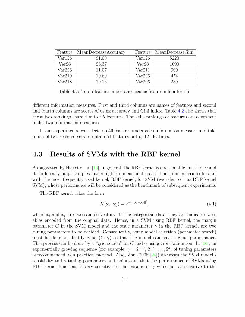
Feature MeanDecreaseAccuracy Feature MeanDecreaseGiniVar126 91.00 Var126 5220Var28 26.37 Var28 1090Var226 11.07 Var211 900Var210 10.60 Var226 474Var218 10.18 Var206 239

Table 4.2: Top 5 feature importance scorse from random forests

different information measures. First and third columns are names of features and secondand fourth columns are scores of using accuracy and Gini index. Table 4.2 also shows thatthese two rankings share 4 out of 5 features. Thus the rankings of features are consistentunder two information measures.

In our experiments, we select top 40 features under each information measure and takeunion of two selected sets to obtain 51 features out of 121 features.

4.3 Results of SVMs with the RBF kernel

As suggested by Hsu et el. in [16], in general, the RBF kernel is a reasonable first choice andit nonlinearly maps samples into a higher dimensional space. Thus, our experiments startwith the most frequently used kernel, RBF kernel, for SVM (we refer to it as RBF kernelSVM), whose performance will be considered as the benchmark of subsequent experiments.

The RBF kernel takes the form

K(xi, xj) = e−γ||xi−xj ||2 , (4.1)

where xi and xj are two sample vectors. In the categorical data, they are indicator vari-ables encoded from the original data. Hence, in a SVM using RBF kernel, the marginparameter C in the SVM model and the scale parameter γ in the RBF kernel, are twotuning parameters to be decided. Consequently, some model selection (parameter search)must be done to identify good (C, γ) so that the model can have a good performance.This process can be done by a “grid-search” on C and γ using cross-validation. In [16], anexponentially growing sequence (for example, γ = 2−10, 2−8, . . . , 23) of tuning parametersis recommended as a practical method. Also, Zhu (2008 [24]) discusses the SVM model’ssensitivity to its tuning parameters and points out that the performance of SVMs usingRBF kernel functions is very sensitive to the parameter γ while not as sensitive to the

24

ROC Curve 0.8180

False positive rate

True

pos

itive

rat

e

0.0 0.2 0.4 0.6 0.8 1.0

0.0

0.2

0.4

0.6

0.8

1.0

Precision−Recall 0.4169

Recall

Pre

cisi

on

0.0 0.2 0.4 0.6 0.8 1.0

0.2

0.4

0.6

0.8

1.0

ROC Curve 0.8174

False positive rateTr

ue p

ositi

ve r

ate

0.0 0.2 0.4 0.6 0.8 1.0

0.0

0.2

0.4

0.6

0.8

1.0


Recall

Pre

cisi

on

0.0 0.2 0.4 0.6 0.8 1.0

0.2

0.4

0.6

0.8

1.0

ROC Curve 0.8152

False positive rate

True

pos

itive

rat

e

0.0 0.2 0.4 0.6 0.8 1.0

0.0

0.2

0.4

0.6

0.8

1.0


RecallP

reci

sion

0.0 0.2 0.4 0.6 0.8 1.0

0.2

0.4

0.6

0.8

1.0

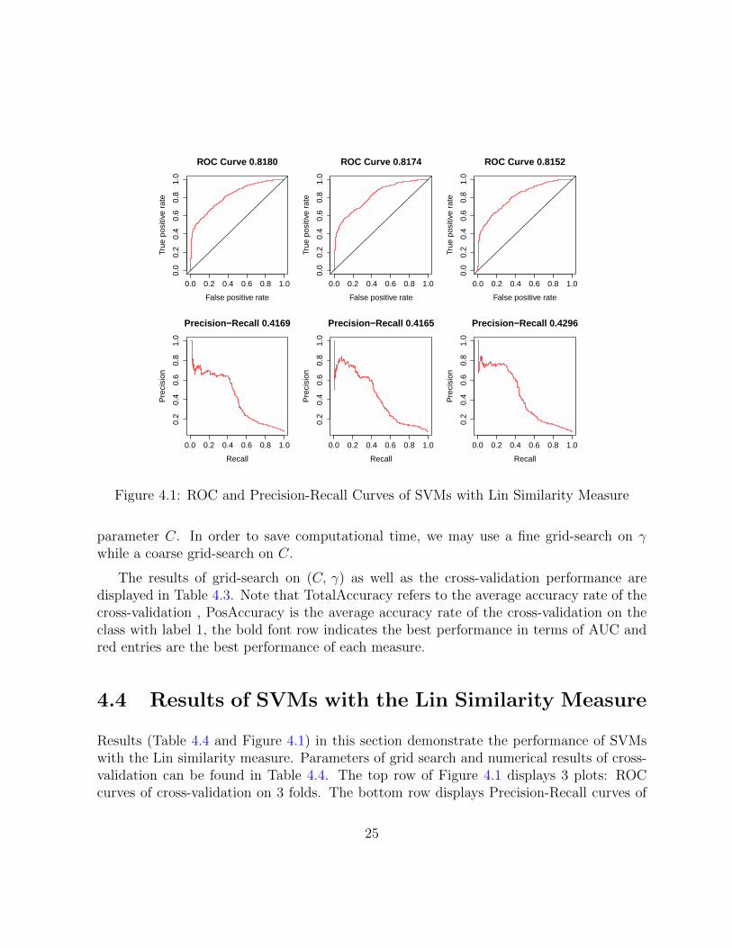
Figure 4.1: ROC and Precision-Recall Curves of SVMs with Lin Similarity Measure

parameter C. In order to save computational time, we may use a fine grid-search on γwhile a coarse grid-search on C.

The results of grid-search on (C, γ) as well as the cross-validation performance aredisplayed in Table 4.3. Note that TotalAccuracy refers to the average accuracy rate of thecross-validation , PosAccuracy is the average accuracy rate of the cross-validation on theclass with label 1, the bold font row indicates the best performance in terms of AUC andred entries are the best performance of each measure.

4.4 Results of SVMs with the Lin Similarity Measure

Results (Table 4.4 and Figure 4.1) in this section demonstrate the performance of SVMswith the Lin similarity measure. Parameters of grid search and numerical results of cross-validation can be found in Table 4.4. The top row of Figure 4.1 displays 3 plots: ROCcurves of cross-validation on 3 folds. The bottom row displays Precision-Recall curves of

25

AUC TotalAccuracy PosAccuracy AP C γ0.6646 0.9262 0.0022 0.1425 1 20

0.7223 0.9301 0.1022 0.2590 1 2−2

0.7552 0.9338 0.2011 0.3457 1 2−4

0.7737 0.9344 0.2293 0.3571 1 2−6

0.7772 0.9268 0.0838 0.3008 1 2−8

0.7782 0.9230 0.0098 0.2959 1 2−9

0.7793 0.9247 0.0054 0.2889 1 2−10

0.7751 0.9257 0.0011 0.2823 1 2−11

0.6640 0.9262 0.0022 0.1423 0.1 20

0.7221 0.9298 0.0935 0.2579 0.1 2−2

0.7549 0.9334 0.2011 0.3443 0.1 2−4

0.7737 0.9344 0.2250 0.3572 0.1 2−6

0.7741 0.9254 0.0577 0.2956 0.1 2−8

0.7759 0.9234 0.0218 0.2853 0.1 2−9

0.7709 0.9250 0.0044 0.2562 0.1 2−10

0.7668 0.9256 0.0022 0.2227 0.1 2−11

0.6583 0.9262 0.0022 0.1379 0.01 20

0.7207 0.9299 0.0924 0.2552 0.01 2−2

0.7550 0.9338 0.2087 0.3449 0.01 2−4

0.7726 0.9340 0.2283 0.3577 0.01 2−6

0.7705 0.9250 0.0294 0.2747 0.01 2−8

0.7624 0.9249 0.0011 0.2310 0.01 2−9

0.7584 0.9256 0.0000 0.2018 0.01 2−10

0.7497 0.9261 0.0000 0.2050 0.01 2−11

Table 4.3: Performance of RBF kernel SVMs. The bold font row indicates the best per-formance in terms of AUC and red entries are the best performance under each measure.

26

AUC TotalAccuracy PosAccuracy AP C0.4999 0.9264 0 - 2−7

0.5000 0.9264 0 - 2−7.5

0.8057 0.9405 0.4011 0.4213 2−8

0.8042 0.9405 0.3924 0.4181 2−8.5

0.8067 0.9397 0.3772 0.4155 2−9

0.8079 0.9398 0.3609 0.4223 2−9.5

0.8119 0.9393 0.3370 0.4180 2−10

0.8169 0.9370 0.2848 0.4210 2−10.5

0.8141 0.9357 0.2468 0.4139 2−11

0.8124 0.9350 0.2152 0.4109 2−11.5

0.8039 0.9310 0.1121 0.3944 2−12

Table 4.4: Performance of SVMs with Lin similarity measure. The bold font row indicatesthe best performance in terms of AUC and red entries are the best performance under eachmeasure.

3 folds. And the title of each plot gives information of AUC or AP based on the curve.

In the table, AUC is the area under the ROC curve shown in Figure 4.1. Since it isa portion of the area of the unit square, its value is always between 0 and 1. A randomguessing produces the diagonal line between (0, 0) and (1, 1) on the ROC curve, whichgives 0.5, the worst AUC. A value of 1 gives the perfect AUC. AP is the area under theprecision-recall curve shown in the second row of Figure 4.1. Although the best AP is 1and the worst is 0, in practice, it takes value between 0.2 to 0.5.

In an ROC curve, the Y axis is the true positive rate which can be viewed as the benefitand X axis is the false positive rate which can be viewed as the cost of a classification model.We prefer a higher benefit with lower cost, which means a higher ROC curve when thefalse positive rate is low. For the precision-recall curve, we expect the curve dropping from1 to 0 as slow as possible to cover a larger area bounded by the X axis and the curve.

4.5 Results of the Ensemble Selection Method

Unlike single SVM models, which can only be optimized to one performance evaluationmeasure, the ensemble selection method is allowed to be optimized to arbitrary performancemetrics. Similarity measures listed in Table 3.1 with parameters in Table 4.4 are usedto train the base SVM models of the model library. Then the ensemble is built via the

27

ROC Curve 0.8255

False positive rate

True

pos

itive

rat

e

0.0 0.2 0.4 0.6 0.8 1.0

0.0

0.2

0.4

0.6

0.8

1.0

ROC Curve 0.8293

False positive rate

True

pos

itive

rat

e

0.0 0.2 0.4 0.6 0.8 1.0

0.0

0.2

0.4

0.6

0.8

1.0

ROC Curve 0.8294


ue p

ositi

ve r

ate

0.0 0.2 0.4 0.6 0.8 1.0

0.0

0.2

0.4

0.6

0.8

1.0


Recall

Pre

cisi

on

0.0 0.2 0.4 0.6 0.8 1.0

0.2

0.4

0.6

0.8

1.0


Recall

Pre

cisi

on

0.0 0.2 0.4 0.6 0.8 1.0

0.2

0.4

0.6

0.8

1.0


Recall

Pre

cisi

on

0.0 0.2 0.4 0.6 0.8 1.0

0.2

0.4

0.6

0.8

1.0

Figure 4.2: ROC and Precision-Recall Curves of Ensemble Selection Method

28

Ensemble Selection on AUCAUC TotalAccuracy PosAccuracy Precision #model

Fold1 0.82552 0.8977 0.5229 0.4132 5

Fold2 0.8293 0.7798 0.6895 0.4186 8

Fold3 0.8294 0.7186 0.7565 0.4388 7

Avg 0.8281 0.7987 0.6563 0.4235 6.7

Ensemble Selection on PrecisionAUC TotalAccuracy PosAccuracy Precision #model

Fold1 0.8185 0.9013 0.5098 0.4407 5

Fold2 0.8229 0.5460 0.8954 0.4302 10

Fold3 0.8241 0.6380 0.8247 0.4613 7

Avg 0.8218 0.6951 0.7433 0.4440 7.3

Table 4.5: Performance of the Ensemble Selection Method. The bold font row indicatesthe best performance in terms of AUC.

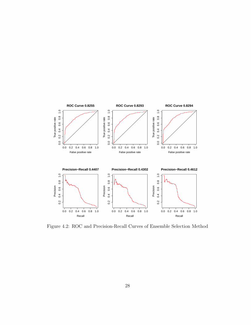
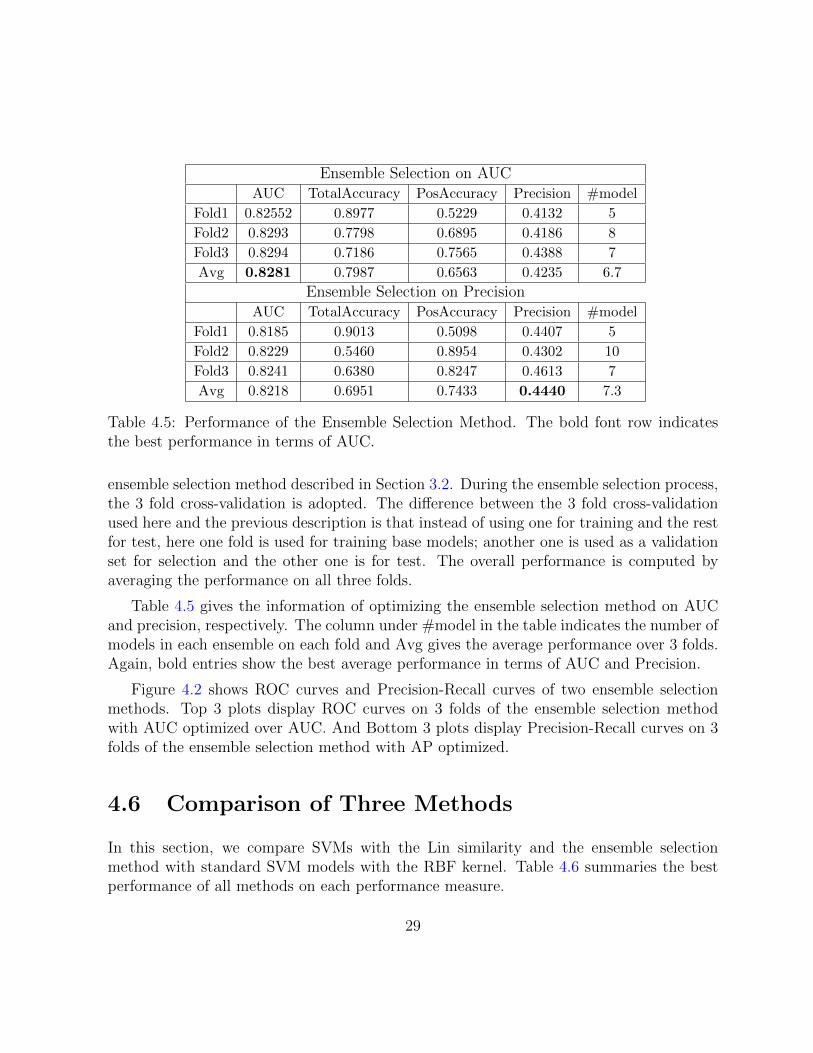
ensemble selection method described in Section 3.2. During the ensemble selection process,the 3 fold cross-validation is adopted. The difference between the 3 fold cross-validationused here and the previous description is that instead of using one for training and the restfor test, here one fold is used for training base models; another one is used as a validationset for selection and the other one is for test. The overall performance is computed byaveraging the performance on all three folds.

Table 4.5 gives the information of optimizing the ensemble selection method on AUCand precision, respectively. The column under #model in the table indicates the number ofmodels in each ensemble on each fold and Avg gives the average performance over 3 folds.Again, bold entries show the best average performance in terms of AUC and Precision.

Figure 4.2 shows ROC curves and Precision-Recall curves of two ensemble selectionmethods. Top 3 plots display ROC curves on 3 folds of the ensemble selection methodwith AUC optimized over AUC. And Bottom 3 plots display Precision-Recall curves on 3folds of the ensemble selection method with AP optimized.

4.6 Comparison of Three Methods

In this section, we compare SVMs with the Lin similarity and the ensemble selectionmethod with standard SVM models with the RBF kernel. Table 4.6 summaries the bestperformance of all methods on each performance measure.

29

ROC Curve 0.8255

False positive rate

True

pos

itive

rat

e

0.0 0.2 0.4 0.6 0.8 1.0

0.0

0.2

0.4

0.6

0.8

1.0

ROC Curve 0.8293

False positive rate

True

pos

itive

rat

e

0.0 0.2 0.4 0.6 0.8 1.0

0.0

0.2

0.4

0.6

0.8

1.0

ROC Curve 0.8294


ue p

ositi

ve r

ate

0.0 0.2 0.4 0.6 0.8 1.0

0.0

0.2

0.4

0.6

0.8

1.0


Recall

Pre

cisi

on

0.0 0.2 0.4 0.6 0.8 1.0

0.2

0.4

0.6

0.8

1.0


Recall

Pre

cisi

on

0.0 0.2 0.4 0.6 0.8 1.0

0.2

0.4

0.6

0.8

1.0


Recall

Pre

cisi

on

0.0 0.2 0.4 0.6 0.8 1.0

0.2

0.4

0.6

0.8

1.0

Figure 4.3: ROC and Precision-Recall Curves of the Ensemble Selection Method

30

Method AUC TotalAccuracy PosAccuracy APRBF kernel 0.7793 0.9338 0.2293 0.3571Lin kernel 0.8169 0.9405 0.4021 0.4222

EnsembleAUC 0.8281 0.7987 0.6563 0.4235EnsembleAP 0.8218 0.6951 0.7433 0.44402

RandomForest 0.8380 0.8272 0.6022 0.4303

Table 4.6: Best performance of RBF kernel, Lin similarity measure kernel SVMs, ensembleselection method and random forest

As mentioned before, the performance of the RBF kernel may be considered as bench-mark of the performance of kernels. Compared with the RBF kernel, the kernel with Linsimilarity measure yields a better performance on all performance measures listed in Table4.3 – 4.6. Especially, keeping the same total accuracy level, the kernel with Lin similaritymeasure dramatically improves accuracy (75%) on the minority class and thus performswell on both AUC and AP.

With the benefit of optimizing performance to arbitrary performance metric, ensemblemethods not only consistently outperform the SVM with RBF kernel on AUC and AP,but also significantly improve accuracy on the minority class even compared with the Linsimilarity kernel SVM. In addition, because of a diverse collection of similarity measures,the ensemble selection approach performs slightly better than random forests in terms ofaccuracy of the minority class.

31

Chapter 5

Conclusion

This paper has presented a novel use of kernels based on data-driven similarity measuresto dealing with categorical features for SVMs. In order to combine benefits of similaritymeasures, we have applied the ensemble selection method to build up an ensemble tooptimize over several performance metrics.

Unlike standard kernels like RBF, when computing similarity measure between samples,our kernel is more closed to a semi-supervised approach that involves the information fromboth labeled and unlabeled data. The ensemble selection method uses the forward stepwiseapproach to select base models for the metrics that we wish to optimize.

Compared with the benchmark — RBF kernel, the results have shown that our ap-proaches are able to improve the performance on all the metrics we used. Especially,keeping other performance measures at the same high level, ensemble selection methodcan significantly increase prediction accuracy on the minority class which is much moredifficult to be predicted when classes are unbalanced.

Possible extension includes developing new similarity measures and introducing differ-ent weight to each selected feature.

32

References

[1] Shigeo Abe. Support vector machines for pattern classification. Springer, 2010.

[2] Michael J Berry and Gordon S Linoff. Data mining techniques: for marketing, sales,and customer relationship management. Wiley. com, 2004.

[3] Shyam Boriah, Varun Chandola, and Vipin Kumar. Similarity measures for categoricaldata: A comparative evaluation. red, 30(2):3, 2008.

[4] Leo Breiman. Classification and regression trees. CRC press, 1993.

[5] Leo Breiman. Bagging predictors. Machine learning, 24(2):123–140, 1996.

[6] Leo Breiman. Random forests. Machine learning, 45(1):5–32, 2001.

[7] Rich Caruana, Alexandru Niculescu-Mizil, Geoff Crew, and Alex Ksikes. Ensembleselection from libraries of models. In Proceedings of the twenty-first internationalconference on Machine learning, page 18. ACM, 2004.

[8] Chih-Chung Chang and Chih-Jen Lin. Libsvm: a library for support vector machines.ACM Transactions on Intelligent Systems and Technology (TIST), 2(3):27, 2011.

[9] Sheng Chen, CFN Cowan, and PM Grant. Orthogonal least squares learning algorithmfor radial basis function networks. Neural Networks, IEEE Transactions on, 2(2):302–309, 1991.

[10] Tom Fawcett. An introduction to roc analysis. Pattern recognition letters, 27(8):861–874, 2006.

[11] Jerome Friedman, Trevor Hastie, and Robert Tibshirani. Additive logistic regression:a statistical view of boosting (with discussion and a rejoinder by the authors). Theannals of statistics, 28(2):337–407, 2000.

33

[12] David W Goodall. A new similarity index based on probability. Biometrics, pages882–907, 1966.

[13] Jiawei Han, Micheline Kamber, and Jian Pei. Data mining: concepts and techniques.Morgan kaufmann, 2006.

[14] Trevor Hastie, Robert Tibshirani, Jerome Friedman, and James Franklin. The ele-ments of statistical learning: data mining, inference and prediction. The MathematicalIntelligencer, 27(2):83–85, 2005.

[15] Douglas M Hawkins. The problem of overfitting. Journal of chemical information andcomputer sciences, 44(1):1–12, 2004.

[16] Chih-Wei Hsu, Chih-Chung Chang, Chih-Jen Lin, et al. A practical guide to supportvector classification, 2003.

[17] Risi Imre Kondor and John Lafferty. Diffusion kernels on graphs and other discreteinput spaces. In ICML, volume 2, pages 315–322, 2002.

[18] Dekang Lin. An information-theoretic definition of similarity. In ICML, volume 98,pages 296–304, 1998.

[19] Huma Lodhi, Craig Saunders, John Shawe-Taylor, Nello Cristianini, and ChrisWatkins. Text classification using string kernels. The Journal of Machine Learn-ing Research, 2:419–444, 2002.

[20] Marvin Minsky and Papert Seymour. Perceptrons. 1969.

[21] Bernhard Schlkopf and Alexander J Smola. Learning with kernels: support vectormachines, regularization, optimization, and beyond. Cambridge: TheMITPress, 2002.

[22] Bernhard Scholkopf, Christopher JC Burges, and Alexander J Smola. Advances inkernel methods: support vector learning. The MIT press, 1999.

[23] Ingo Steinwart, Don Hush, and Clint Scovel. An explicit description of the reproducingkernel hilbert spaces of gaussian rbf kernels. Information Theory, IEEE Transactionson, 52(10):4635–4643, 2006.

[24] Mu Zhu. Kernels and ensembles. The American Statistician, 62(2), 2008.

34

data-driven kernels for support vector machines · data-driven kernels for support vector machines...

Documents