Data Detection, Channel Equalisation &

Estimation

EIT 140, tom<AT>eit.lth.se

Coherent and noncoherent detection

absolute modulation −→ coherent detection

differential modulation −→ noncoherent detection

symbol i − 1

symbol i

channel

channel i − 1

channel i

equalizer

i is an index in time (multicarrier symbol No.) or frequency (subcarrier No.)

Coherent and noncoherent detection, cont’d

absolute modulation −→ coherent detection

information lies in the choice of symbol from constellationrequires channel equalisation and estimationperformance depends on channel estimation (which itself depends oncorrelation between channel coefficients)

differential modulation −→ noncoherent detection

information lies in the difference between two consecutive symbolsno need for channel equalisation and estimation (fewer pilots)depending on channel’s coherence properties, differential modulationin

time (compare to same subcarrier in previous multicarrier-symbol)frequency (compare to adjacent subcarrier in samemulticarrier-symbol)

performance depends on correlation between channel coefficientshigher BER compared to coherent demodulation but less overhead(fewer pilots)

OFDM: differential modulation in time

multicarrier symbol No. n −→

←−

subcarrierNo.k

diff. modulation in time

→→→→→→→→→→→→→→→→→

diff. phase modulation: xk,n=e jϕk,nH [k,n]=ck,ne

jφk,n

−→ yk,n

=ck,nej(ϕk,n+φk,n)+wk,n

noncoherent detection in time: x̂ k,n = yk,n

y ∗k,n−1

x̂ k,n=ck,nck,n−1e j(ϕk,n−ϕk,n−1+φk,n−φk,n−1)+wk,nw∗k,n−1+wk,ny

∗k,n−1+w∗k,n−1yk,n

Grey subcarriers are pilots providing an initial phase reference

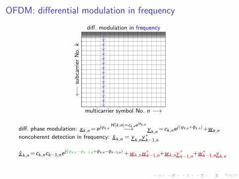
OFDM: differential modulation in frequency

multicarrier symbol No. n −→

←−

subcarrierNo.k

diff. modulation in frequency

↓↓↓↓↓↓↓↓↓↓↓↓↓↓↓

diff. phase modulation: xk,n=e jϕk,nH [k,n]=ck,ne

jφk,n

−→ yk,n

=ck,nej(ϕk,n+φk,n)+wk,n

noncoherent detection in frequency: x̂ k,n = yk,n

y ∗k−1,n

x̂ k,n=ck,nck−1,nej(ϕk,n−ϕk−1,n+φk,n−φk−1,n)+wk,nw

∗k−1,n+wk,ny

∗k−1,n+w∗k−1,nyk,n

Least squares (LS) approach

Consider the modely = Ax, (1)

where A ∈ Rm×n is a strictly skinny (m > n) deterministic and known

coefficient matrix, y is a deterministic and known vector and x is unknown.

for most y, there is no x that solves (1) (by solves we mean exactly)

An approach to find a “good” approximation x that approximately solves (1) isthe following

define the error e = Ax− y

find xLS that minimises the Euclidean norm ‖e‖2=√eTe of the error, i.e.,

xLS = argminx‖e‖2 (2)

The approximate “solution” xLS is called least squares solution. Note:

minimising ‖e‖2 corresponds to minimising the energy of the error

parameter x and error e are deterministic—least squares is a deterministicapproach

LS geometric interpretation

The least squares solution xLS minimises the Euclidean distance between AxLSand y

R(A) is the n-dimensional subspace spanned by the columns of A

Ax is a projection of the point y onto R(A) (and thus lies in R(A))among all projections, the orthogonal projection AxLS minimises ‖e‖2

R(A)

y

e

AxLS

LS solution

assume that A is full rank (rank{A} = n)

xLS minimises both ‖e‖2 and ‖e‖22‖e‖22= eTe = xTATAx− xTATy− yTAx+ yTy = xTATAx− 2xTATy+ yTy

to minimise ‖e‖22, we set the gradient ∇x ‖e‖22 to zero

∇x ‖e‖22= 2ATAx− 2ATy!= 0

this yields the so-called normal equations ATAx = ATy

since A is full rank, ATA is nonsingular n× n matrix

the least squares solution is thus

xLS =(

ATA)−1

ATy

similarly, in the complex-valued case we obtain: xLS =(

AHA)−1

AHy

Minimum mean square error (MMSE) estimation

Consider a length-n parameter vector x to be estimated from a length-mobservation vector y

assumption: parameters are realisation of a random vector x withcovariance matrix Cxx = E

{xxT

}

An approach to find a “good” linear estimate x̂ = Gy of x is the following

define the error e = x− x̂ = x−Gy

find xMMSE that minimises the mean of the squared error, i.e.,

xMMSE = argminx̂

E{

‖e‖22}

(3)

xMMSE is called minimum mean square error (MMSE) estimate. Note:

parameter x and error e are stochastic—MMSE is a Bayesian estimationapproach

Assumption: all random variables/vector have mean zero (correlation and covarianceare identical)

MMSE geometric interpretation

Scalar case (n = 1): the MMSE estimate xMMSE minimises the Euclideandistance between xMMSE and x

components of y span an m-dimensional subspace YgTy is a projection of x onto Y (and thus lies in Y)among all projections, the orthogonal projection xMMSE = gMMSE

Ty of xonto Y minimises the mean of ‖e‖2x − gMMSE

Ty is orthogonal to Y , which implies E{(x − gMMSE

Ty)y}= 0

Y

x

xMMSE

MMSE solution

xMMSE has to fulfil E{(x − gMMSE

Ty)y}= 0

consequently, E {yx} − E{gMMSE

Tyy}= E {yx}

︸ ︷︷ ︸

cyx

−E{

yyT}

︸ ︷︷ ︸

Cyy

gMMSE = 0

this yields the so-called Wiener-Hopf equations CyygMMSE = cyx

whose solution is gMMSE = C−1yycyx

the MMSE solution is thus

xMMSE = cyxTC−1

yyy

similarly, in the complex-valued vector-case we obtain: xMMSE = CHyxC

−1yyy

Applications for LS and MMSE

data estimation (equalisation)

channel estimation

channel shortening

Linear equalisation

x

w

x̂y

RH RZadd ZremH G

transmitter channel receiver

y = RZrem

(

HZaddRHx+w

)

= RZremHZaddRH

︸ ︷︷ ︸

A

x+RZremw︸ ︷︷ ︸

w′

for L ≥ M: ZremHZadd is circulant and RZremHZaddRH is diagonal

linear equalisation: x̂ = Gy

depending on the design of G, we distinguish

least-squares design −→ zero-forcing equaliser xZF = GZFy

MMSE design −→ MMSE equaliser xMMSE = GMMSEy

Least squares design: zero-forcing equaliser

xLS = (AHA)−1AH

︸ ︷︷ ︸

GLS

y

if A is diagonal, GLS is diagonal

zero-forcing equaliser GLS for a given channel H, is the inverse A−1 (ifthis inverse exists, i.e., if A has no zeros on its diagonal)

if the channel exhibits spectral nulls on the FFT grid (A has zeros on itsdiagonal), a pseudo inverse can be constructed

Note:

LS design does not consider the noise in the model −→ xLS can bearbitrarily off (noise amplification)

the zero-forcing equaliser tries to force the interference to be zeroregardless of the consequences caused by the noise

MMSE design: MMSE equaliser

xMMSE = CxxAH(

ACxxAH +Cw′w′

)−1

︸ ︷︷ ︸

GMMSE

y

Cxx = E{xxH

}is the covariance matrix of the transmit data

Cw′w′ = E{w′w′H

}is covariance matrix of the received noise

if A, Cxx and Cw′w′ are diagonal, GMMSE is diagonal

Cw′w′ “stabilises” the inverse (even if A has zeros on its diagonal)

Note:

instead of fighting exclusively the interference, the MMSE equaliser aimsat minimising the mean of the (total) squared error

prior information (covariance matrices of transmit signal and noise,respectively) is required

Multicarrier equalisation

probably the biggest advantage of OFDM: equalisation is trivial

channel partitioning leads to parallel narrow-band frequency-flatsubchannels

multiplication of each subchannel by a scalar does not change thesub-channel SNR

still, equalisation of the complex-valued multiplication factors caused byeach subchannel is necessary before detection

example: Maximum-likelihood symbol detection for QAM

nevertheless, in order to do this per-subchannel equalisation (thecorresponding device is often referred to as frequency-domain equaliser(FEQ)), we need to know these complex-valued coefficients: → channelestimation (is not trivial)

Frequency-domain equalisation (FEQ)

As long as L ≥ M holds, multicarrier equalisation reduces to multiplication witha complex scalar per subchannel.The ZF equaliser written in DFT-domain is

HZF[k ] =1

H [k ]=

H∗[k ]|H [k ]|2 , k = 0, . . . ,N − 1,

where k denotes the subcarrier (subchannel) index.The MMSE equaliser in DFT-domain is given by

HMMSE[k ] =H∗[k ]

|H [k ]|2 +Cw′w′ [k , k ], k = 0, . . . ,N − 1,

where Cw′w′ [k , k ] describes the noise power (or equivalently, the noise variance

for zero-mean noise) of the kth subchannel.

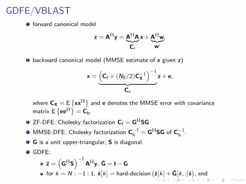
GDFE/VBLAST

forward canonical model

z = AHy = AHA︸ ︷︷ ︸

Cf

x+AHw︸ ︷︷ ︸

w′

,

backward canonical model (MMSE estimate of x given z)

x =(

Cf + (N0/2)C−1x

)−1

︸ ︷︷ ︸

Cb

z+ e,

where Cx = E{xxH

}and e denotes the MMSE error with covariance

matrix E{eeH

}= Cb.

ZF-DFE: Cholesky factorization Cf = GHSG

MMSE-DFE: Cholesky factorization C−1b = GHSG of C−1

b .

G is a unit upper-triangular, S is diagonal.

GDFE:

z̃ =(

GHS)−1

AHy, G̃ = I−G

for k = N : −1 : 1, x̂[k ] = hard-decision(z̃[k ] + G̃[k , :]x̂

), end

Scalar precoding: principle of Tomlinson/Harashima

transmit modM (x + q) instead of x + q

perform modulo-operation modM (y)

q

q

+1

+3

+5

+7

+9

+11

−1−3−5−7−9−11

channel modM

Vector precoding

1 Factorize P = QR. (Q is unitary. R is unit upper-triangular)

ttP R Q

p

pQH

2 Recursive substitution. Example:

1 −1 2 10 1 3 20 0 1 20 0 0 1

︸ ︷︷ ︸

R

+1−3+1+3

︸ ︷︷ ︸

t

=

9673

−→

1 −1 2 10 1 3 20 0 1 20 0 0 1

︸ ︷︷ ︸

R

+25+13−7+3

︸ ︷︷ ︸

t

=

1−2−13

3 An additive component p can be easily included

Channel estimation

pilot-based (time-frequency grid)

pilot allocation must fulfil Nyquist theorem in time and frequency:

pilot-spacing in time ∆t must fulfil ∆t < Tcoh = 1/Bdop

pilot-spacing in frequency ∆f must fulfil ∆f < Bcoh = 1/τmax

one-/two-dimensional estimation techniquesdifferent pilot allocation for continuous (broadcast) and packettransmission

decision-directed

uses only a few known symbols at the beginning of transmissionfurther channel estimation is based on (hopefully) correct datadecisions which allows channel estimation using all causal subcarriersperformance depends again on coherence properties of the channel

Examples for pilot allocation

continuous transmission

multicarrier symbol No. −→

←−

subcarrierNo.

packet transmission

multicarrier symbol No. −→←−

subcarrierNo.

Light-grey subcarriers are used for synchronisation

Time-domain equalisation (TEQ)

whole multicarrier concept falls apart if L < M (intersymbol interference(ISI) and inter-carrier interference (ICI))

100 L/(N + L)% of the achievable rate (or equivalently, of the transmitpower) are inherently wasted −→ the smaller L = M, the better

goal of time-domain “equalisation”: shorten the channel dispersion M toM1 < M

s(n)

channel receiver

TEQ

DFThTEQ(n)R ′[k ]

h(n)

w(n)

r(n) r ′(n)

TEQ design

The desired result of the linear convolution of the transversal filterhEQ(n), n = 0, . . . ,K of length K + 1 and the channel can be described usingconvolution matrix notation:

0...0

r ′(0)r ′(1)...

r ′(M1)0...0

=

h(0) 0 . . . 0

h(1) h(0)...

h(1). . . 0

.... . . h(0)

h(1)h(M)

h(M)...

.... . .

0 . . . 0 h(M)

hEQ(0)hEQ(1)

...hEQ(K )

omit the rows that yield r ′(n), 1 ≤ n ≤ M1 (“don’t care”)

keep the row yielding r ′(0) and fix that coefficient

TEQ design: least-squares problem

Least-squares problem formulation:

0...010...0

︸︷︷︸

r′

=

h(0) 0 . . . 0

h(1) h(0)...

.... . . h(0)

h(M ′) h(1)h(M)

h(M)...

.... . .

0 . . . 0 h(M)

︸ ︷︷ ︸

H′

hEQ(0)hEQ(1)

...hEQ(K )

︸ ︷︷ ︸

hEQ

+e,

We are looking for a solution hEQ that makes the error e as small as possibleThis operation has to be repeated for all possible positions of the 1 in r′.

TEQ design: solution of the least-squares problem

Least-squares problem formulation:

r′ = H′hEQ + e

Find the hEQ that minimises the squared Euclidean norm ||e||22 of the error e.The impulse response that yields this minimum is denoted

hTEQ = argminhEQ

||e||22. (4)

Equation (4) formulates the least squares problem

the parameter hEQ is deterministic

we did not invoke any statistics

there is no expectation in (4)

The solution to (4) is given by

hTEQ =(

H′HH′)−1

H′Hr′.

Summary

1 Coherent and noncoherent detection

absolute modulation −→ channel equalisation, coherent detectiondifferential modulation −→ noncoherent detection

2 Estimation principles

least squaresMMSE

3 Data estimation

least-squares design −→ zero-forcing equaliserMMSE design −→ MMSE equaliserequalisation in OFDM: one multiplication per subcarrierGDFE, THP, TEQ