data-derived pointwise consistency - upmcplc/data2015/anantharam2015.pdf · outline insurance...
TRANSCRIPT

Outline Insurance Compression Learning
Data-derived pointwise consistency
Venkat AnantharamUniversity of California, Berkeley
Challenges for Optimization in Data ScienceUniversite Pierre et Marie Curie – Paris 6
July 1 -2, 2015
joint work with Narayana Prasad SanthanamUniversity of Hawaii, Manoa

Outline Insurance Compression Learning
Outline
1 Insurance
2 Compression
3 Learning

Outline Insurance Compression Learning
Outline
1 Insurance
2 Compression
3 Learning
Outline Insurance Compression Learning
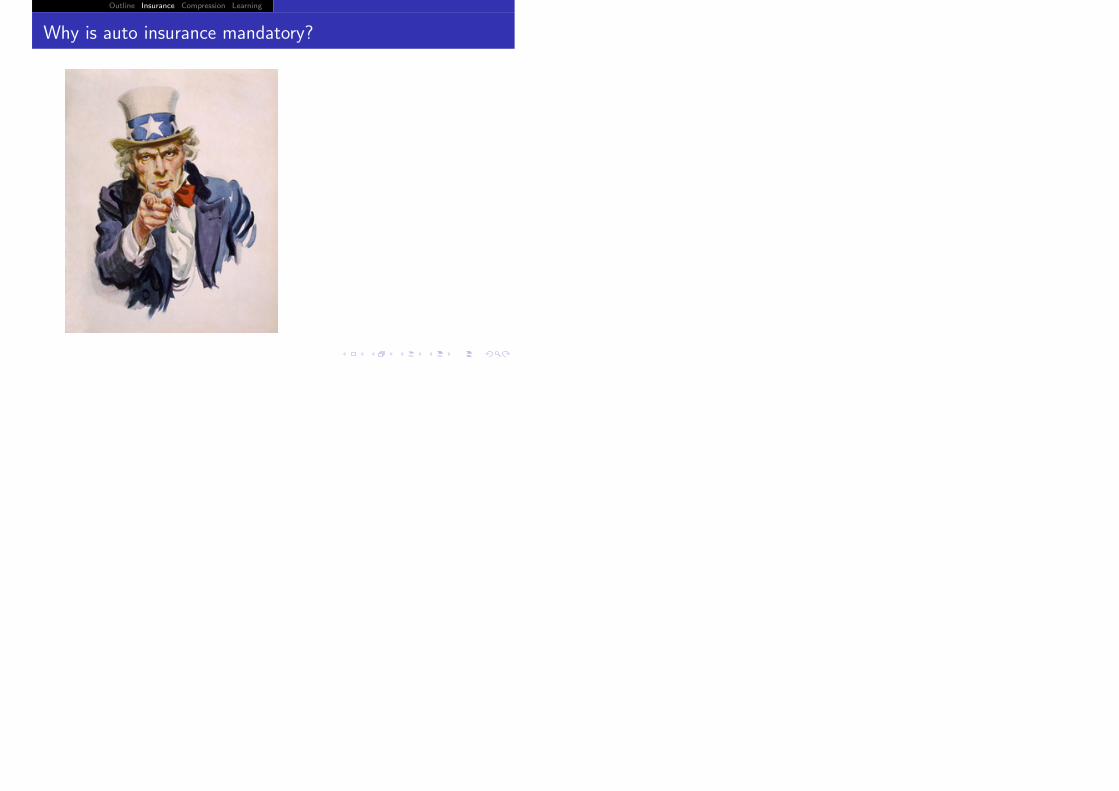
Why is auto insurance mandatory?

Outline Insurance Compression Learning
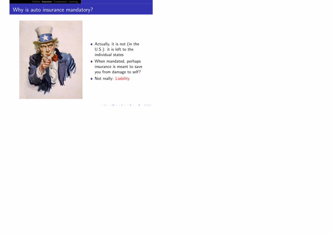
Why is auto insurance mandatory?
Actually, it is not (in theU.S.): it is left to theindividual states

Outline Insurance Compression Learning
Why is auto insurance mandatory?
Actually, it is not (in theU.S.): it is left to theindividual states
When mandated, perhapsinsurance is meant to saveyou from damage to self?
Outline Insurance Compression Learning
Why is auto insurance mandatory?
Actually, it is not (in theU.S.): it is left to theindividual states
When mandated, perhapsinsurance is meant to saveyou from damage to self?
Not really: Liability

Outline Insurance Compression Learning
What makes the insurance industry tick?
Outline Insurance Compression Learning
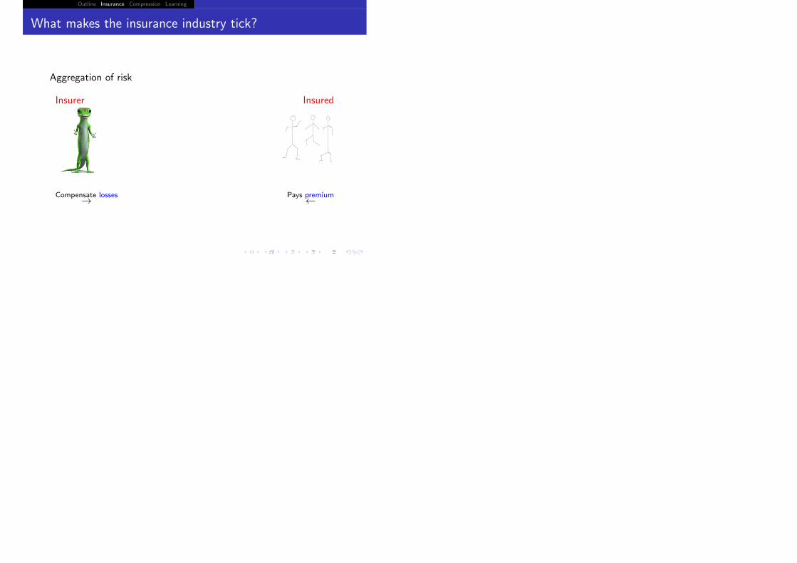
What makes the insurance industry tick?
Aggregation of risk
Insurer Insured
Compensate losses→ Pays premium←

Outline Insurance Compression Learning
How to set the premiums?

Outline Insurance Compression Learning
How to set the premiums?
Probabilistic approaches [Lundberg, Cramer, .. ]
Outline Insurance Compression Learning
How to set the premiums?
Probabilistic approaches [Lundberg, Cramer, .. ]Parametric: assume there is enough data to build a realisticmodel for the distribution of losses
Outline Insurance Compression Learning
How to set the premiums?
Probabilistic approaches [Lundberg, Cramer, .. ]Parametric: assume there is enough data to build a realisticmodel for the distribution of lossesThe insurer starts with some initial capital, losses with theknown distribution occur at the times of some point process,premiums are set based on the model, avoiding bankruptcy iscertainly the most basic goal.

Outline Insurance Compression Learning
How we got started on this work

Outline Insurance Compression Learning
How we got started on this work
The availability of insurance enables risk taking and so is adriver of innovation
Outline Insurance Compression Learning
How we got started on this work
The availability of insurance enables risk taking and so is adriver of innovation
So one should encourage the emergence of an insuranceindustry
Outline Insurance Compression Learning
How we got started on this work
The availability of insurance enables risk taking and so is adriver of innovation
So one should encourage the emergence of an insuranceindustry
But there are markets where not enough data to build areliable loss model, e.g. cyberinsurance.

Outline Insurance Compression Learning
Cyberinsurance
Outline Insurance Compression Learning
Cyberinsurance
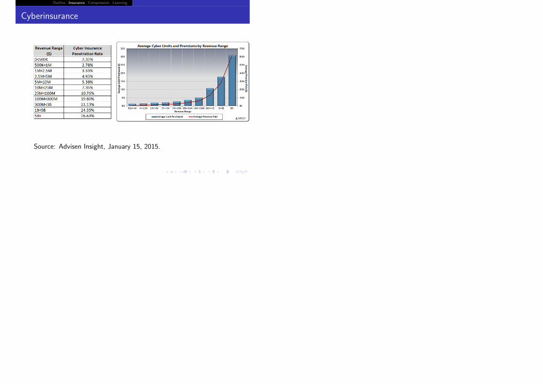
Source: Advisen Insight, January 15, 2015.

Outline Insurance Compression Learning
Our approach to the problem

Outline Insurance Compression Learning
Our approach to the problem
Insurer
The insurer adopts anonparametric model forlosses

Outline Insurance Compression Learning
Our approach to the problem
Insurer
The insurer adopts anonparametric model forlosses
The loss distribution isonly assumed to be amember of a class P ofloss distributions

Outline Insurance Compression Learning
Our approach to the problem
Insurer
The insurer adopts anonparametric model forlosses
The loss distribution isonly assumed to be amember of a class P ofloss distributions
The premium settingstrategy should workuniversally over lossdistributions in this class

Outline Insurance Compression Learning
Our approach to the problem
Insurer
The insurer adopts anonparametric model forlosses
The loss distribution isonly assumed to be amember of a class P ofloss distributions
The premium settingstrategy should workuniversally over lossdistributions in this class
We ask: which classes Pare insurable?

Outline Insurance Compression Learning
Nonparametric Approach to Insurance
Insurer Insured
Compensate losses→Pays premium←
• Charges premiums such thatbuilt up reserves Φt+1,Φt+2, . . . Incurs loss X1,X2, . . .

Outline Insurance Compression Learning
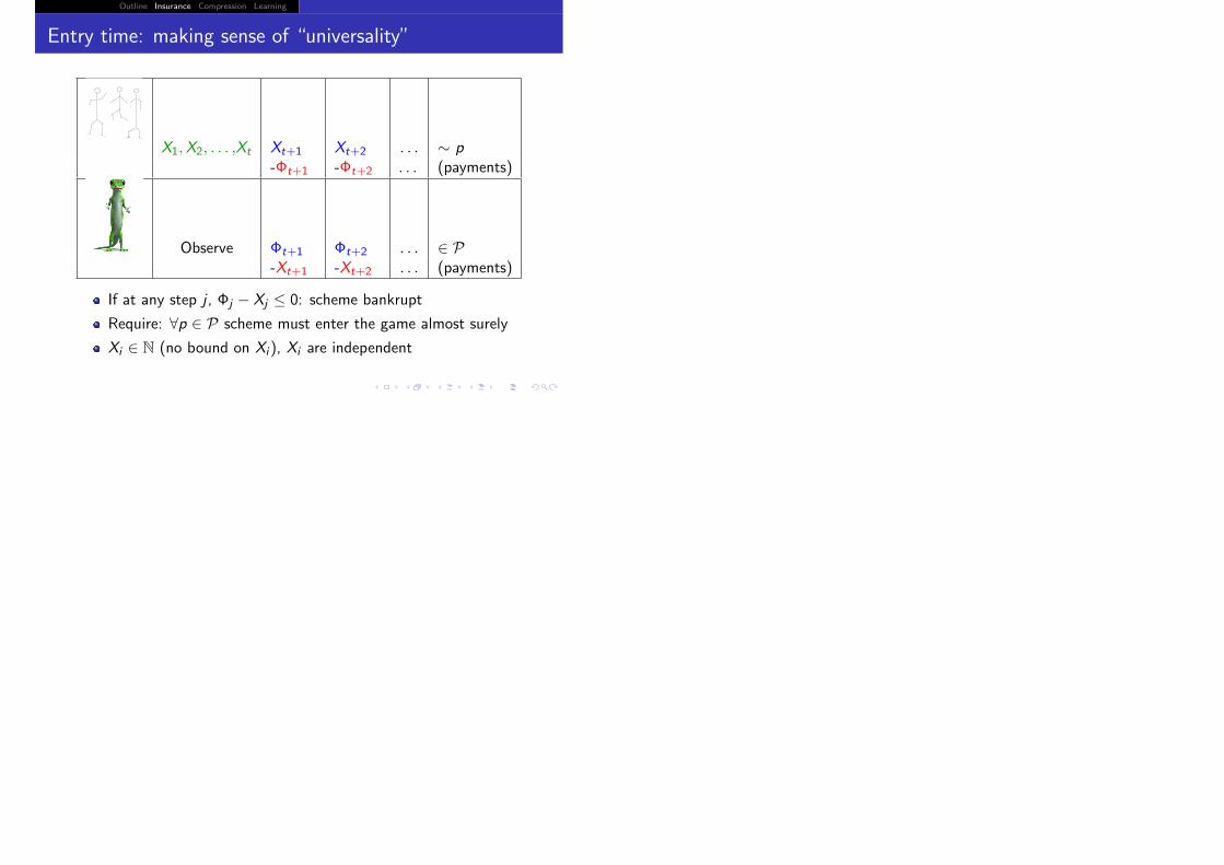
Entry time: making sense of “universality”
X1,X2, . . . ,Xt Xt+1 Xt+2 . . . ∼ p-Φt+1 -Φt+2 . . . (payments)
Observe Φt+1 Φt+2 . . . ∈ P-Xt+1 -Xt+2 . . . (payments)

Outline Insurance Compression Learning
Entry time: making sense of “universality”
X1,X2, . . . ,Xt Xt+1 Xt+2 . . . ∼ p-Φt+1 -Φt+2 . . . (payments)
Observe Φt+1 Φt+2 . . . ∈ P-Xt+1 -Xt+2 . . . (payments)
If at any step j , Φj − Xj ≤ 0: scheme bankrupt

Outline Insurance Compression Learning
Entry time: making sense of “universality”
X1,X2, . . . ,Xt Xt+1 Xt+2 . . . ∼ p-Φt+1 -Φt+2 . . . (payments)
Observe Φt+1 Φt+2 . . . ∈ P-Xt+1 -Xt+2 . . . (payments)
If at any step j , Φj − Xj ≤ 0: scheme bankrupt
Require: ∀p ∈ P scheme must enter the game almost surely
Xi ∈ N (no bound on Xi ), Xi are independent

Outline Insurance Compression Learning
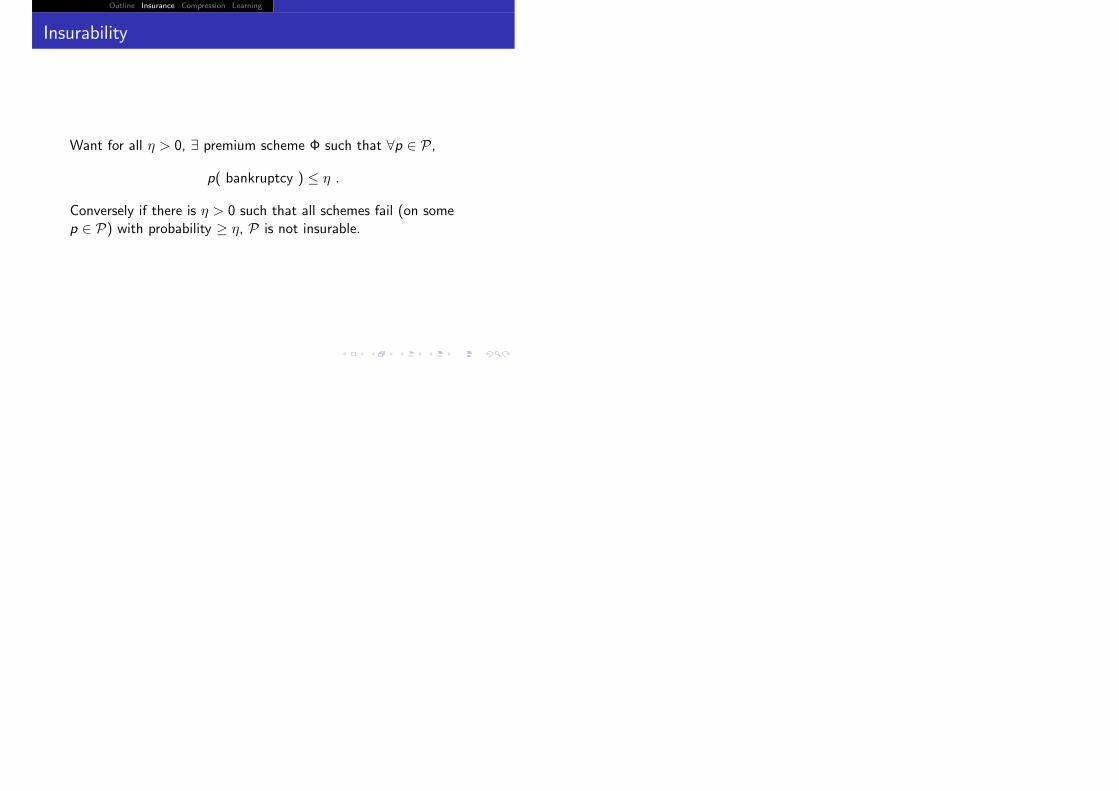
Insurability
Want for all η > 0, ∃ premium scheme Φ such that ∀p ∈ P,
p( bankruptcy ) ≤ η .
Outline Insurance Compression Learning
Insurability
Want for all η > 0, ∃ premium scheme Φ such that ∀p ∈ P,
p( bankruptcy ) ≤ η .
Conversely if there is η > 0 such that all schemes fail (on somep ∈ P) with probability ≥ η, P is not insurable.
Outline Insurance Compression Learning
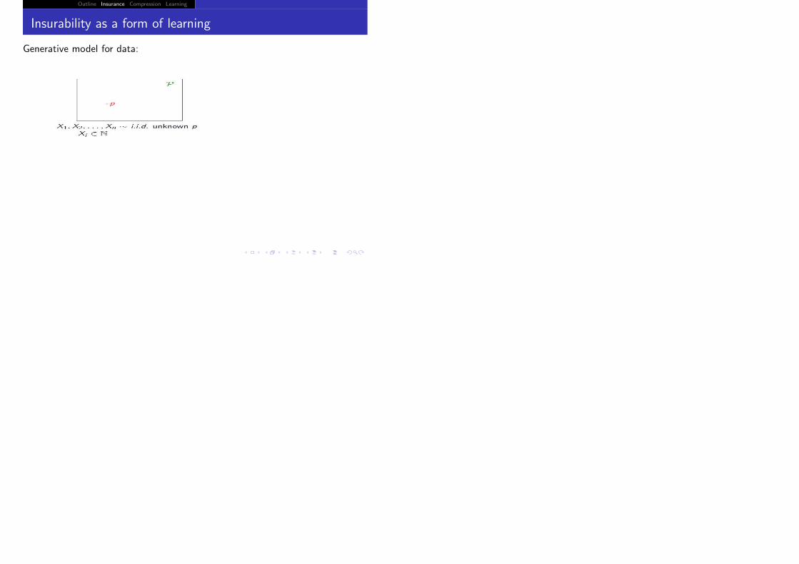
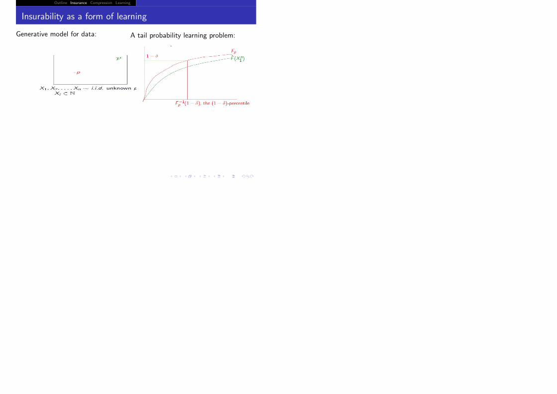
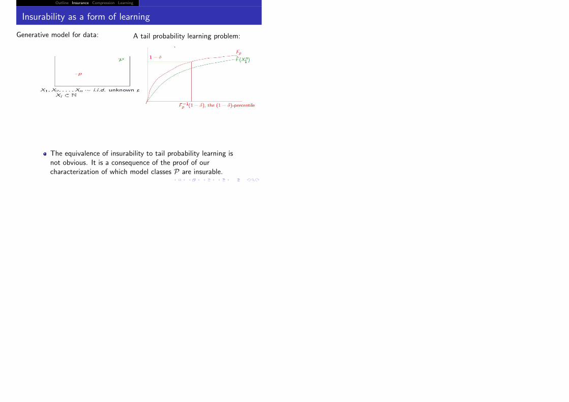
Insurability as a form of learning
Generative model for data:
Outline Insurance Compression Learning
Insurability as a form of learning
Generative model for data: A tail probability learning problem:
Outline Insurance Compression Learning
Insurability as a form of learning
Generative model for data: A tail probability learning problem:
The equivalence of insurability to tail probability learning isnot obvious. It is a consequence of the proof of ourcharacterization of which model classes P are insurable.

Outline Insurance Compression Learning
Deceptive distributions

Outline Insurance Compression Learning
Deceptive distributions
Let
J(p, q) := D(p�p + q
2) + D(q�p + q
2) .
where
D(p�q) :=�
i
p(i) logp(i)
q(i).
Outline Insurance Compression Learning
Deceptive distributions
Let
J(p, q) := D(p�p + q
2) + D(q�p + q
2) .
where
D(p�q) :=�
i
p(i) logp(i)
q(i).
A probability distribution p ∈ P is called deceptive (for tails) if:
For all � > 0, there exists δ > 0 such that for all x ∈ R, thereexists q ∈ P with
J(p, q) ≤ � ,
andF−1q (1− δ) > x .

Outline Insurance Compression Learning
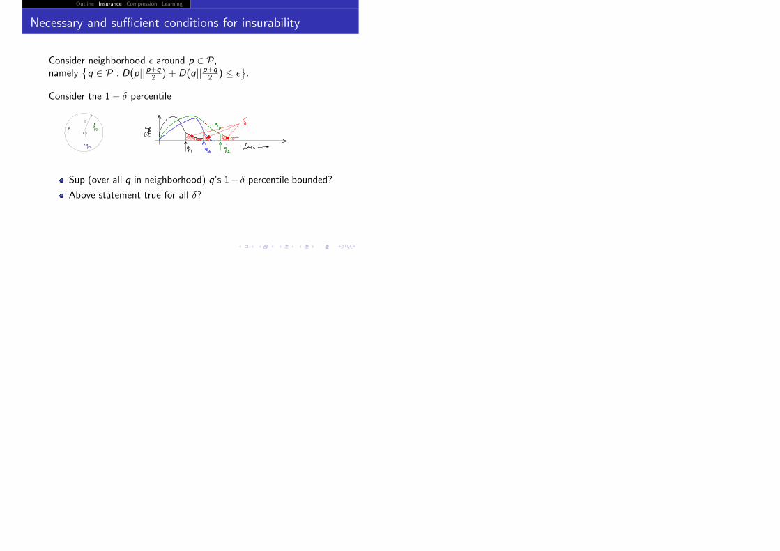
Necessary and sufficient conditions for insurability
Consider neighborhood � around p ∈ P,namely
�q ∈ P : D(p||p+q
2 ) + D(q||p+q2 ) ≤ �
�.

Outline Insurance Compression Learning
Necessary and sufficient conditions for insurability
Consider neighborhood � around p ∈ P,namely
�q ∈ P : D(p||p+q
2 ) + D(q||p+q2 ) ≤ �
�.
Consider the 1− δ percentile

Outline Insurance Compression Learning
Necessary and sufficient conditions for insurability
Consider neighborhood � around p ∈ P,namely
�q ∈ P : D(p||p+q
2 ) + D(q||p+q2 ) ≤ �
�.
Consider the 1− δ percentile
Sup (over all q in neighborhood) q’s 1− δ percentile bounded?
Outline Insurance Compression Learning
Necessary and sufficient conditions for insurability
Consider neighborhood � around p ∈ P,namely
�q ∈ P : D(p||p+q
2 ) + D(q||p+q2 ) ≤ �
�.
Consider the 1− δ percentile
Sup (over all q in neighborhood) q’s 1− δ percentile bounded?
Above statement true for all δ?
Theorem: P is insurable iff ∃ neighborhood around all p ∈ P suchthat the above two conditions are true.

Outline Insurance Compression Learning
Data derived pointwise consistency
Pointwise consistency has two flavors(i) where we cannot tell from data if we are doing well(ii) where we can.

Outline Insurance Compression Learning
Data derived pointwise consistency
Pointwise consistency has two flavors(i) where we cannot tell from data if we are doing well(ii) where we can.
Data derived pointwise consistency
In addition to pointwise consistent estimator, for any givenconfidence 1− η there is a stopping rule that stops universally forall p ∈ P after the estimator starts doing well with confidence> 1− η.

Outline Insurance Compression Learning
Examples
If P is:
The set of all finite support distributions, then it is notinsurable
The set of all uniform distributions, then it is insurable
The set of all monotone distributions (with finite entropy),then it is not insurable
The set of all distributions with a uniformly bounded mean,then it is insurable
The set of all distributions with a finite mean, then it is notinsurable

Outline Insurance Compression Learning
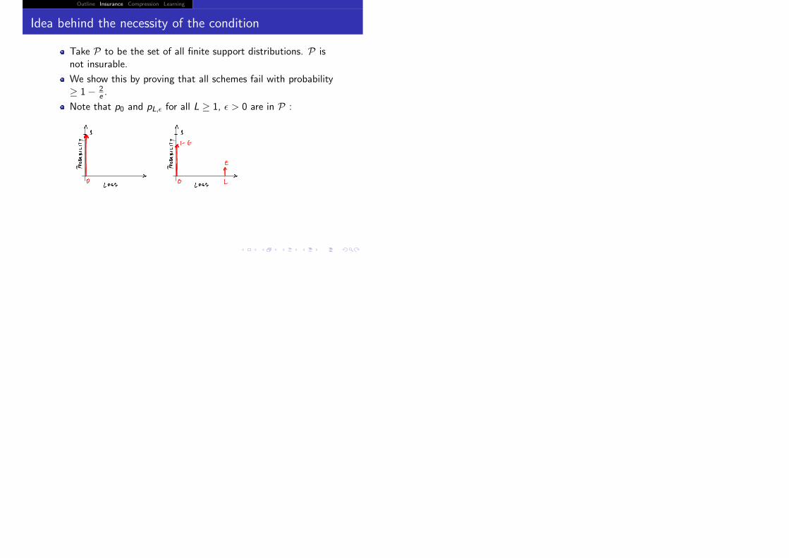
Idea behind the necessity of the condition

Outline Insurance Compression Learning
Idea behind the necessity of the condition
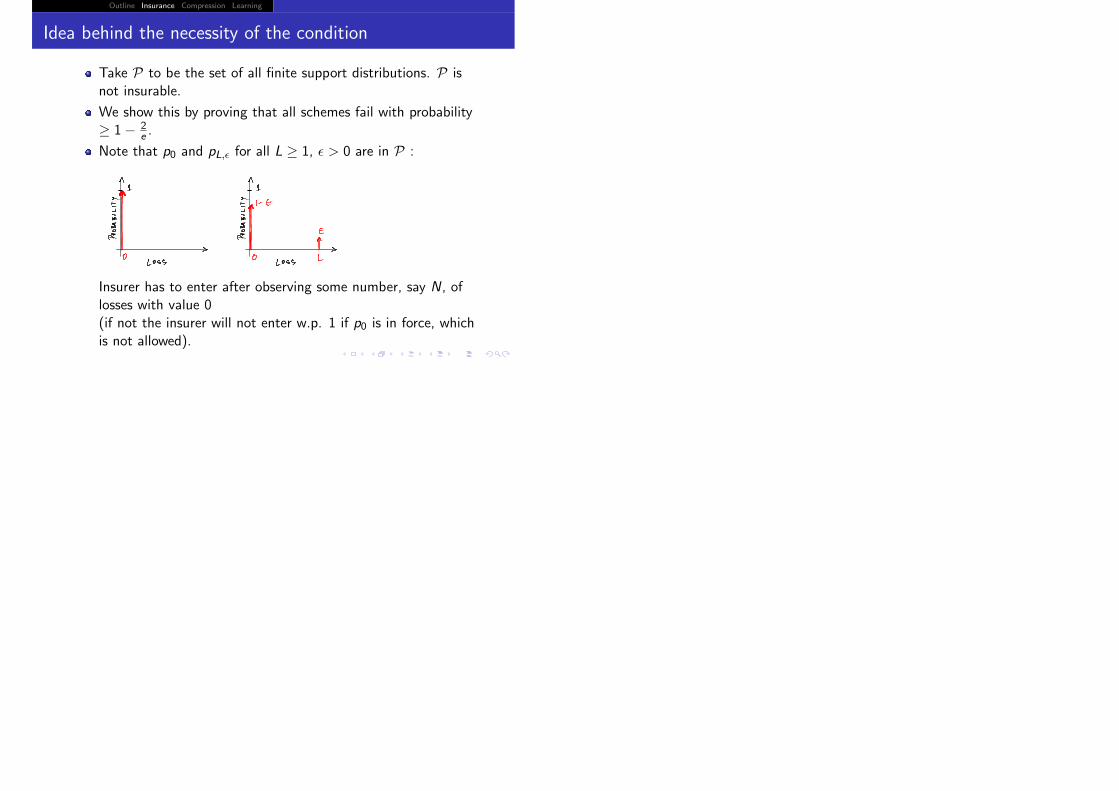
Take P to be the set of all finite support distributions. P isnot insurable.

Outline Insurance Compression Learning
Idea behind the necessity of the condition
Take P to be the set of all finite support distributions. P isnot insurable.
We show this by proving that all schemes fail with probability≥ 1− 2
e .
Outline Insurance Compression Learning
Idea behind the necessity of the condition
Take P to be the set of all finite support distributions. P isnot insurable.
We show this by proving that all schemes fail with probability≥ 1− 2
e .
Note that p0 and pL,� for all L ≥ 1, � > 0 are in P :
Outline Insurance Compression Learning
Idea behind the necessity of the condition
Take P to be the set of all finite support distributions. P isnot insurable.
We show this by proving that all schemes fail with probability≥ 1− 2
e .
Note that p0 and pL,� for all L ≥ 1, � > 0 are in P :
Insurer has to enter after observing some number, say N, oflosses with value 0(if not the insurer will not enter w.p. 1 if p0 is in force, whichis not allowed).

Outline Insurance Compression Learning
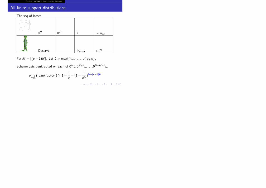
All finite support distributions
The seq of losses
0N 0m ? ∼ pL,�
Observe ΦN+m ∈ P
Fix M = �(e − 1)N�. Let L > max{ΦN+1, . . . ,ΦN+M}.
Scheme gets bankrupted on each of 0NL, 0N+1L, . . . ,0N+M−1L.
pL, 1Ne( bankruptcy ) ≥ (1− 1
Ne)N − (1− 1
Ne)N+M

Outline Insurance Compression Learning
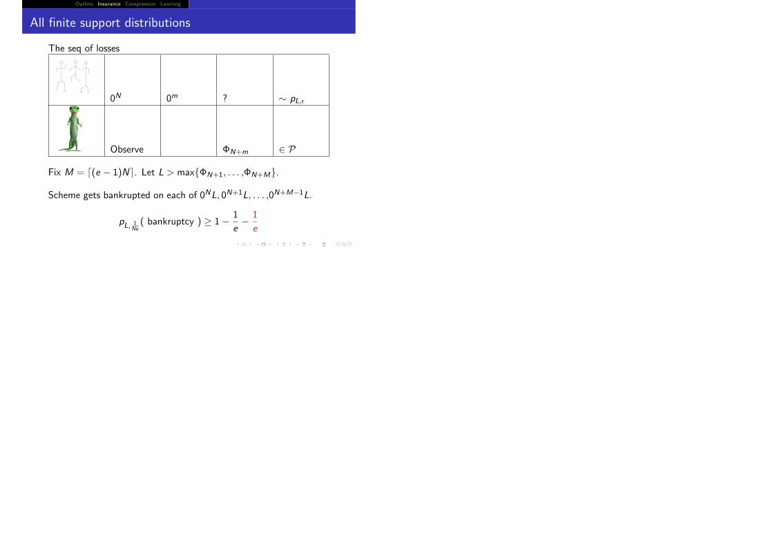
All finite support distributions
The seq of losses
0N 0m ? ∼ pL,�
Observe ΦN+m ∈ P
Fix M = �(e − 1)N�. Let L > max{ΦN+1, . . . ,ΦN+M}.
Scheme gets bankrupted on each of 0NL, 0N+1L, . . . ,0N+M−1L.
pL, 1Ne( bankruptcy ) ≥ 1− N
Ne− (1− 1
Ne)N+M
Outline Insurance Compression Learning
All finite support distributions
The seq of losses
0N 0m ? ∼ pL,�
Observe ΦN+m ∈ P
Fix M = �(e − 1)N�. Let L > max{ΦN+1, . . . ,ΦN+M}.
Scheme gets bankrupted on each of 0NL, 0N+1L, . . . ,0N+M−1L.
pL, 1Ne( bankruptcy ) ≥ 1− 1
e− (1− 1
Ne)N+(e−1)N

Outline Insurance Compression Learning
All finite support distributions
The seq of losses
0N 0m ? ∼ pL,�
Observe ΦN+m ∈ P
Fix M = �(e − 1)N�. Let L > max{ΦN+1, . . . ,ΦN+M}.
Scheme gets bankrupted on each of 0NL, 0N+1L, . . . ,0N+M−1L.
pL, 1Ne( bankruptcy ) ≥ 1− 1
e− (1− 1
Ne)Ne
Outline Insurance Compression Learning
All finite support distributions
The seq of losses
0N 0m ? ∼ pL,�
Observe ΦN+m ∈ P
Fix M = �(e − 1)N�. Let L > max{ΦN+1, . . . ,ΦN+M}.
Scheme gets bankrupted on each of 0NL, 0N+1L, . . . ,0N+M−1L.
pL, 1Ne( bankruptcy ) ≥ 1− 1
e− 1
e

Outline Insurance Compression Learning
Sketch of proof of sufficiency
Outline Insurance Compression Learning
Sketch of proof of sufficiency
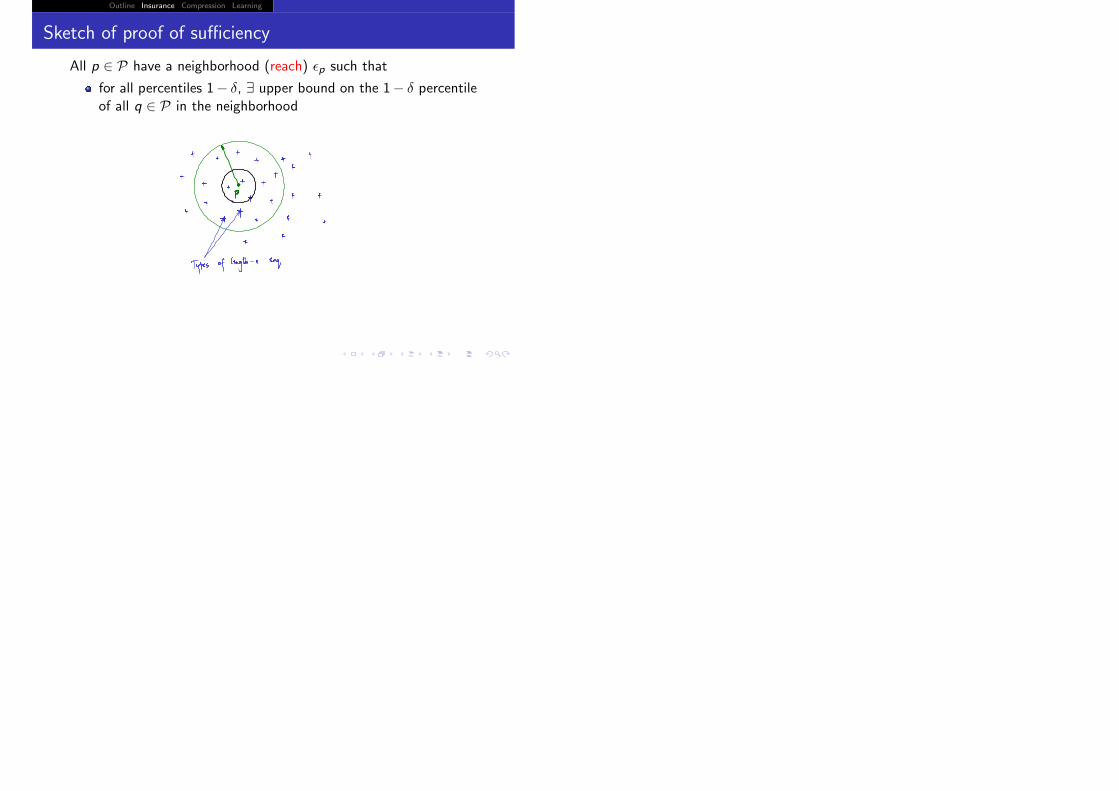
All p ∈ P have a neighborhood (reach) �p such that
for all percentiles 1− δ, ∃ upper bound on the 1− δ percentileof all q ∈ P in the neighborhood

Outline Insurance Compression Learning
Sketch of proof of sufficiency
All p ∈ P have a neighborhood (reach) �p such that
for all percentiles 1− δ, ∃ upper bound on the 1− δ percentileof all q ∈ P in the neighborhood
When p ∈ P is in effect, the insurer observes the type (empiricaldistribution) of the losses to decide what to do.
Outline Insurance Compression Learning
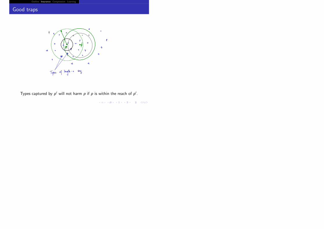
Good traps
Types captured by p� will not harm p if p is within the reach of p�.

Outline Insurance Compression Learning
Bad traps
p generates types captured by hostile p� —but such types have lowprobabilityPutting these together gives a constructive proof for the sufficiencycondition
Outline Insurance Compression Learning
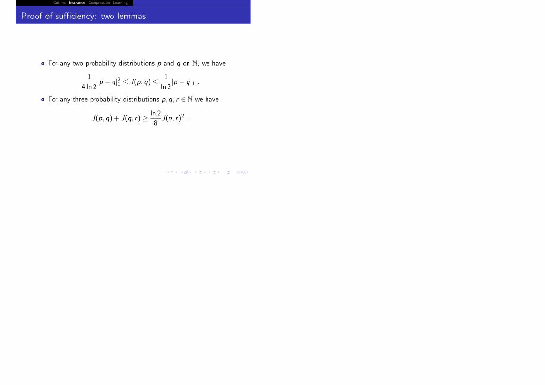
Proof of sufficiency: two lemmas
For any two probability distributions p and q on N, we have
1
4 ln 2|p − q|21 ≤ J(p, q) ≤ 1
ln 2|p − q|1 .
For any three probability distributions p, q, r ∈ N we have
J(p, q) + J(q, r) ≥ ln 2
8J(p, r)2 .

Outline Insurance Compression Learning
Outline
1 Insurance
2 Compression
3 Learning

Outline Insurance Compression Learning
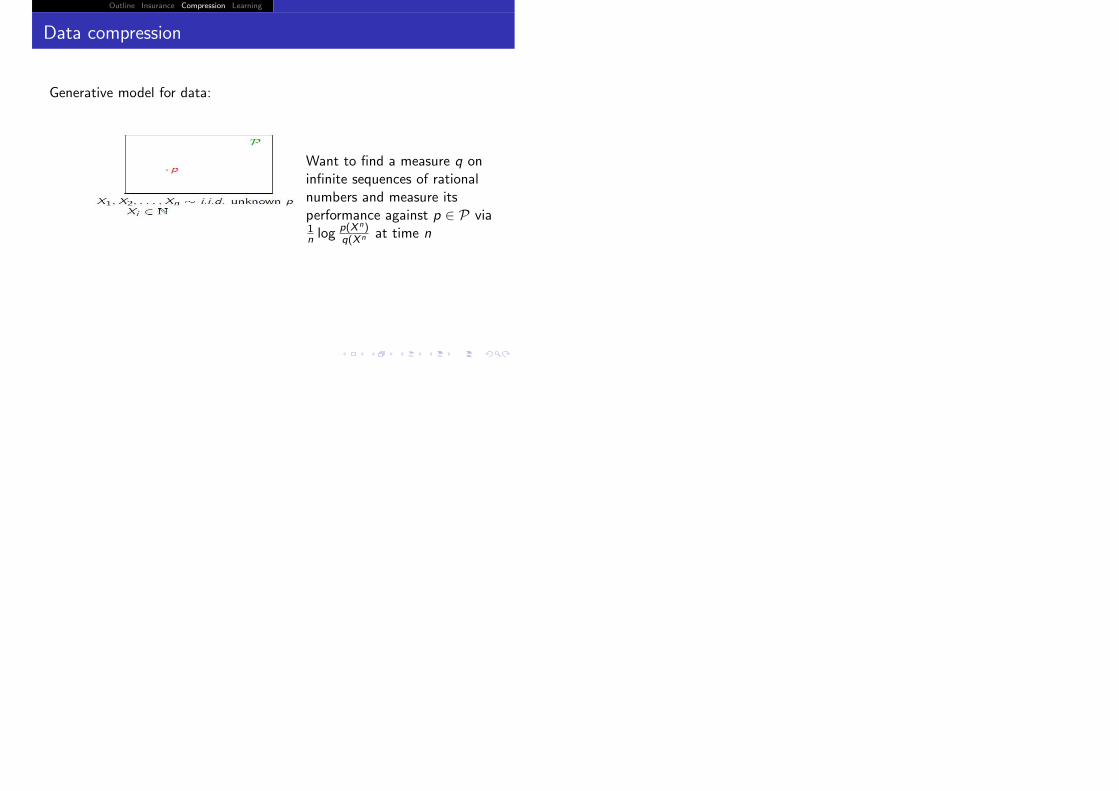
Data compression
Generative model for data:
Outline Insurance Compression Learning
Data compression
Generative model for data:
Want to find a measure q oninfinite sequences of rationalnumbers and measure itsperformance against p ∈ P via1n log
p(Xn)q(Xn at time n

Outline Insurance Compression Learning
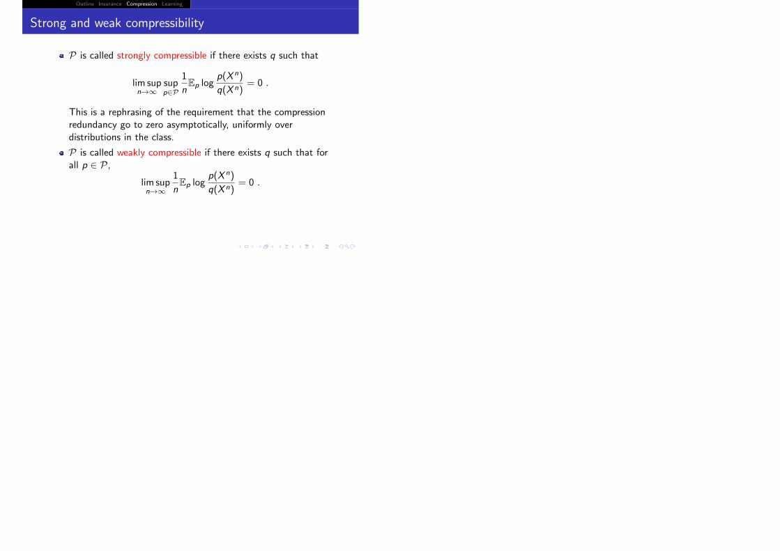
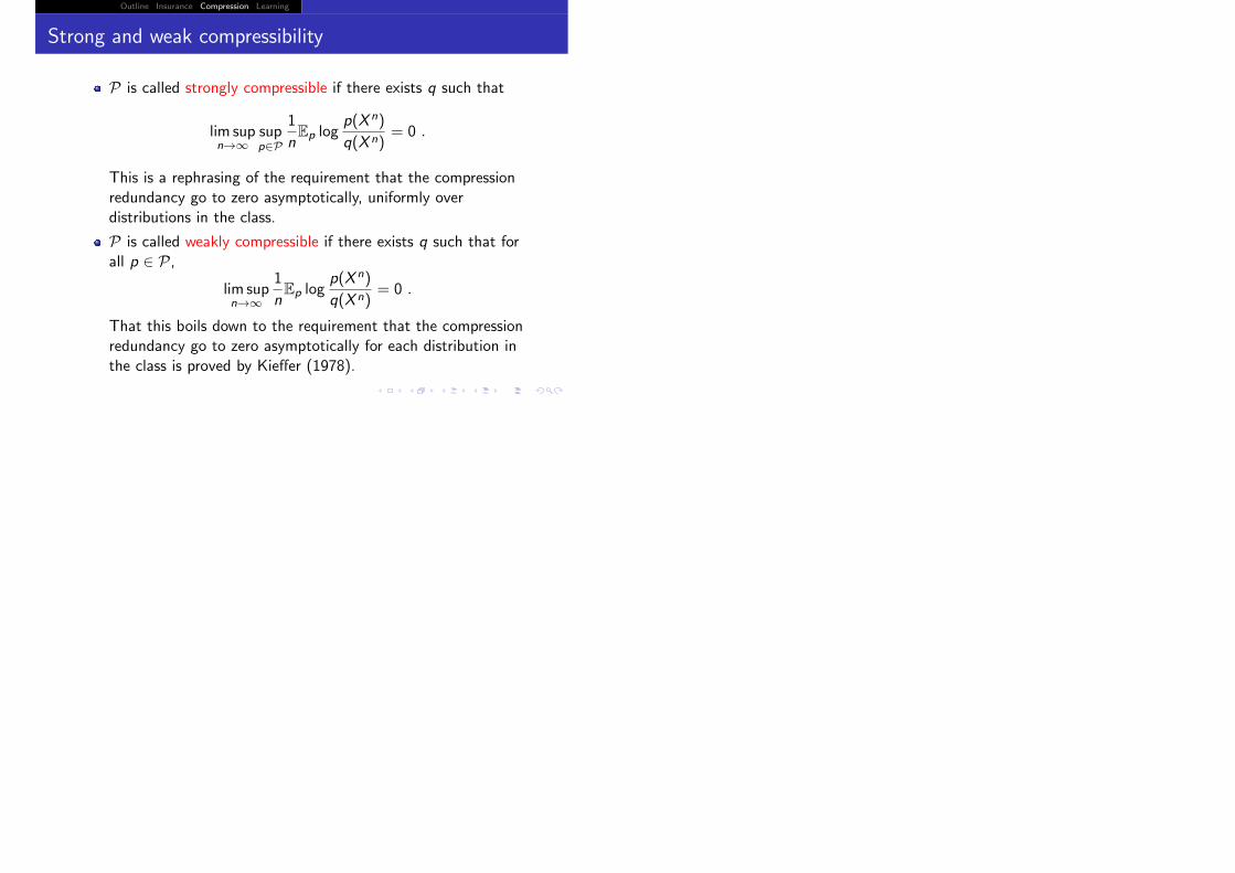
Strong and weak compressibility

Outline Insurance Compression Learning
Strong and weak compressibility
P is called strongly compressible if there exists q such that
lim supn→∞
supp∈P
1
nEp log
p(X n)
q(X n)= 0 .
Outline Insurance Compression Learning
Strong and weak compressibility
P is called strongly compressible if there exists q such that
lim supn→∞
supp∈P
1
nEp log
p(X n)
q(X n)= 0 .
This is a rephrasing of the requirement that the compressionredundancy go to zero asymptotically, uniformly overdistributions in the class.
P is called weakly compressible if there exists q such that forall p ∈ P,
lim supn→∞
1
nEp log
p(X n)
q(X n)= 0 .
That this boils down to the requirement that the compressionredundancy go to zero asymptotically for each distribution inthe class is proved by Kieffer (1978).

Outline Insurance Compression Learning
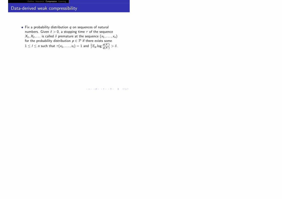
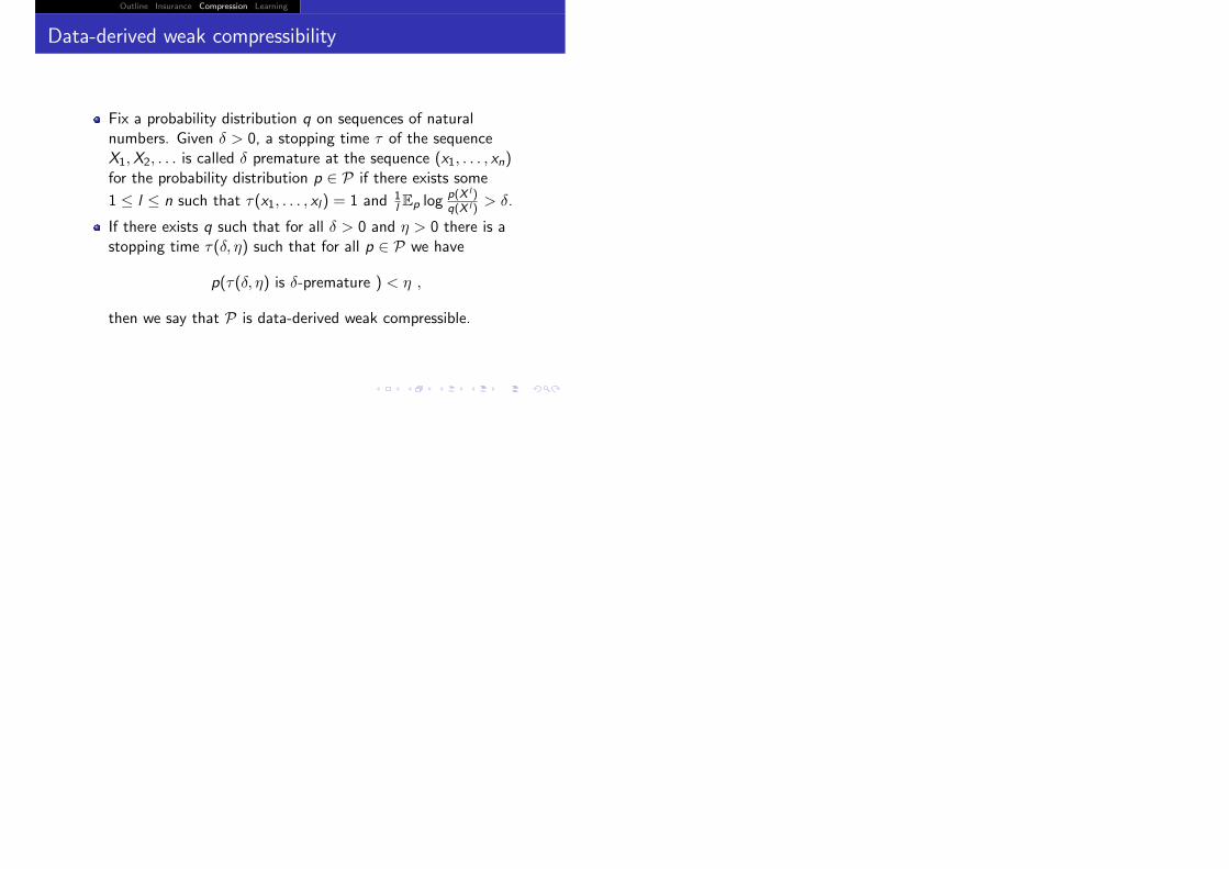
Data-derived weak compressibility
Outline Insurance Compression Learning
Data-derived weak compressibility
Fix a probability distribution q on sequences of naturalnumbers. Given δ > 0, a stopping time τ of the sequenceX1,X2, . . . is called δ premature at the sequence (x1, . . . , xn)for the probability distribution p ∈ P if there exists some
1 ≤ l ≤ n such that τ(x1, . . . , xl) = 1 and 1l Ep log
p(Xl )q(Xl )
> δ.
If there exists q such that for all δ > 0 and η > 0 there is astopping time τ(δ, η) such that for all p ∈ P we have
p(τ(δ, η) is δ-premature ) < η ,
then we say that P is data-derived weak compressible.

Outline Insurance Compression Learning
Reiterating the value of the data derived notion

Outline Insurance Compression Learning
Reiterating the value of the data derived notion
Pointwise consistency has two flavors(i) where we cannot tell from data if we are doing well(ii) where we can.

Outline Insurance Compression Learning
Reiterating the value of the data derived notion
Pointwise consistency has two flavors(i) where we cannot tell from data if we are doing well(ii) where we can.
Data derived pointwise consistency
In addition to pointwise consistent estimator, for any givenconfidence 1− η there is a stopping rule that stops universally forall p ∈ P after the estimator starts doing well with confidence> 1− η.

Outline Insurance Compression Learning
Characterizing data-derived weak compressibility

Outline Insurance Compression Learning
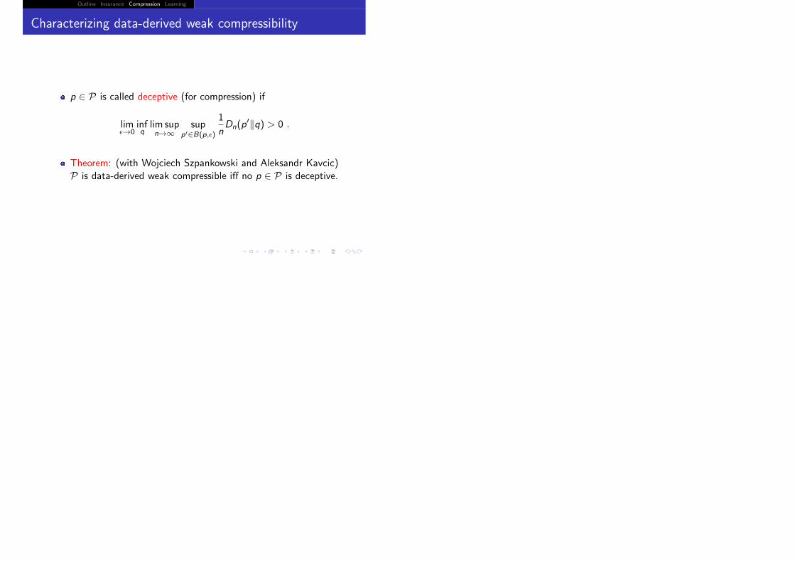
Characterizing data-derived weak compressibility
p ∈ P is called deceptive (for compression) if
lim�→0
infqlim supn→∞
supp�∈B(p,�)
1
nDn(p
��q) > 0 .
Outline Insurance Compression Learning
Characterizing data-derived weak compressibility
p ∈ P is called deceptive (for compression) if
lim�→0
infqlim supn→∞
supp�∈B(p,�)
1
nDn(p
��q) > 0 .
Theorem: (with Wojciech Szpankowski and Aleksandr Kavcic)P is data-derived weak compressible iff no p ∈ P is deceptive.

Outline Insurance Compression Learning
Examples
Outline Insurance Compression Learning
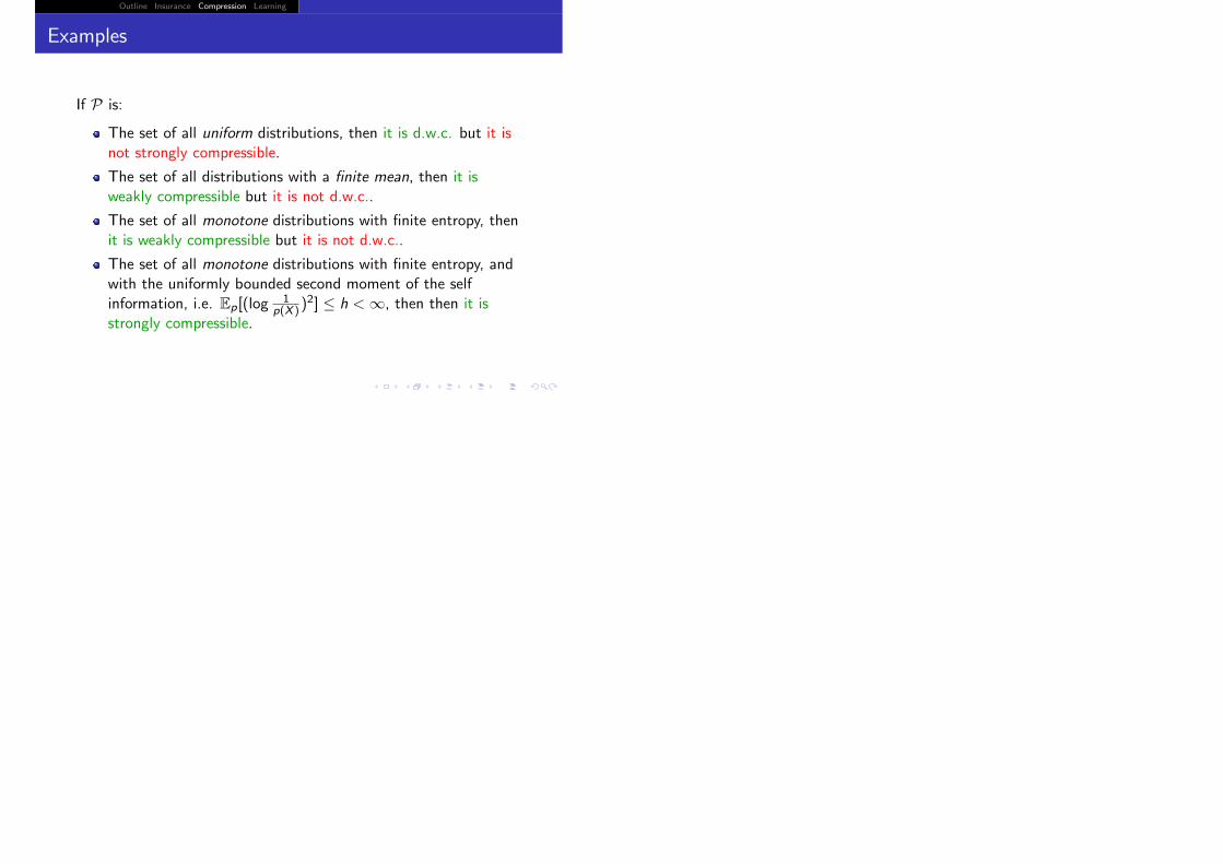
Examples
If P is:
The set of all uniform distributions, then it is d.w.c. but it isnot strongly compressible.
The set of all distributions with a finite mean, then it isweakly compressible but it is not d.w.c..
The set of all monotone distributions with finite entropy, thenit is weakly compressible but it is not d.w.c..
The set of all monotone distributions with finite entropy, andwith the uniformly bounded second moment of the selfinformation, i.e. Ep[(log
1p(X ))
2] ≤ h < ∞, then then it isstrongly compressible.
Outline Insurance Compression Learning
Proofs
Different from, but of the same flavor, as the proofs for theinsurability theorem.

Outline Insurance Compression Learning
Insurability does not imply strong compressibility
The class of all finitely supported uniform distributions, isinsurable but is not strong compressible.

Outline Insurance Compression Learning
Strong compressibility implies insurability
R := infqsupn∈N
supp∈P
log(p(n)
q(n)) < ∞ ,
is achieved by the Shtarkov distribution

Outline Insurance Compression Learning
Strong compressibility implies insurability
R := infqsupn∈N
supp∈P
log(p(n)
q(n)) < ∞ ,
is achieved by the Shtarkov distribution
q∗(n) :=supp∈P p(n)�
n�≥0 supp∈P p(n�).
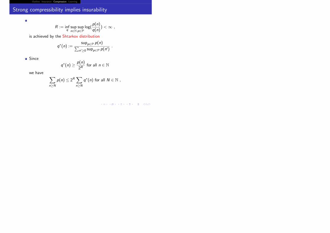
Outline Insurance Compression Learning
Strong compressibility implies insurability
R := infqsupn∈N
supp∈P
log(p(n)
q(n)) < ∞ ,
is achieved by the Shtarkov distribution
q∗(n) :=supp∈P p(n)�
n�≥0 supp∈P p(n�).
Since
q∗(n) ≥ p(n)
2Rfor all n ∈ N
we have �
n≥N
p(n) ≤ 2R�
n≥N
q∗(n) for all N ∈ N ,
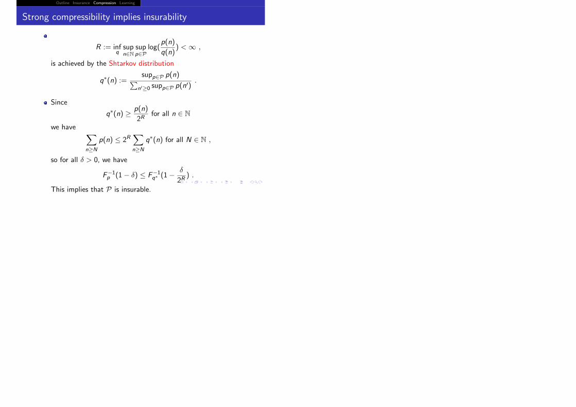
Outline Insurance Compression Learning
Strong compressibility implies insurability
R := infqsupn∈N
supp∈P
log(p(n)
q(n)) < ∞ ,
is achieved by the Shtarkov distribution
q∗(n) :=supp∈P p(n)�
n�≥0 supp∈P p(n�).
Since
q∗(n) ≥ p(n)
2Rfor all n ∈ N
we have �
n≥N
p(n) ≤ 2R�
n≥N
q∗(n) for all N ∈ N ,
so for all δ > 0, we have
F−1p (1− δ) ≤ F−1
q∗ (1− δ
2R) .
This implies that P is insurable.
Outline Insurance Compression Learning
Weak compressibility does not imply insurability
The class of all finite mean distributions, is not insurable butis weakly compressible.

Outline Insurance Compression Learning
Insurability does not imply weak compressibility
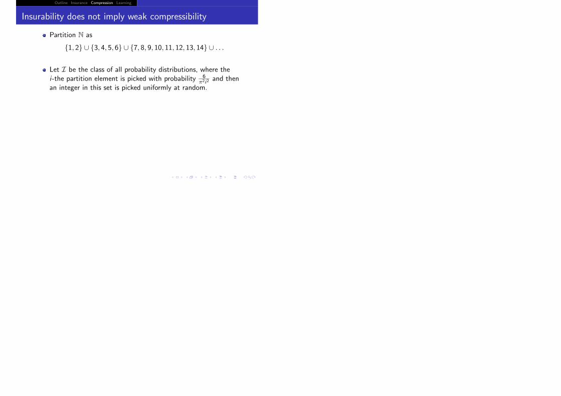
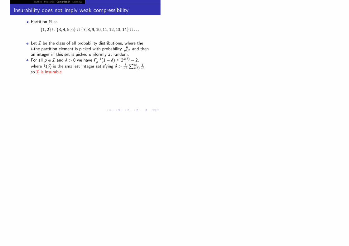
Partition N as
{1, 2} ∪ {3, 4, 5, 6} ∪ {7, 8, 9, 10, 11, 12, 13, 14} ∪ . . .
Outline Insurance Compression Learning
Insurability does not imply weak compressibility
Partition N as
{1, 2} ∪ {3, 4, 5, 6} ∪ {7, 8, 9, 10, 11, 12, 13, 14} ∪ . . .
Let I be the class of all probability distributions, where thei-the partition element is picked with probability 6
π2i2and then
an integer in this set is picked uniformly at random.
For all p ∈ I and δ > 0 we have F−1p (1− δ) ≤ 2k(δ) − 2,
where k(δ) is the smallest integer satisfying δ > 6π2
�∞k(δ)
1i2,
so I is insurable.
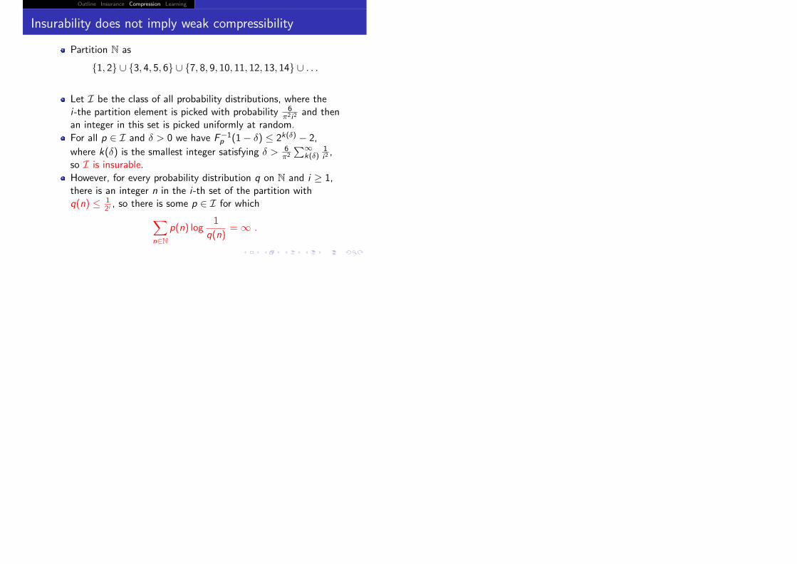
However, for every probability distribution q on N and i ≥ 1,there is an integer n in the i-th set of the partition withq(n) ≤ 1
2i, so there is some p ∈ I for which
�
n∈Np(n) log
1
q(n)= ∞ .
Outline Insurance Compression Learning
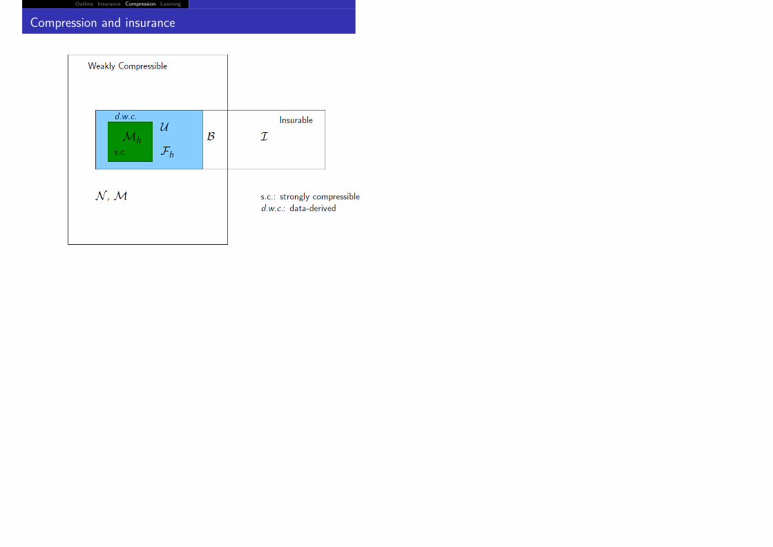
Compression and insurance
Outline Insurance Compression Learning
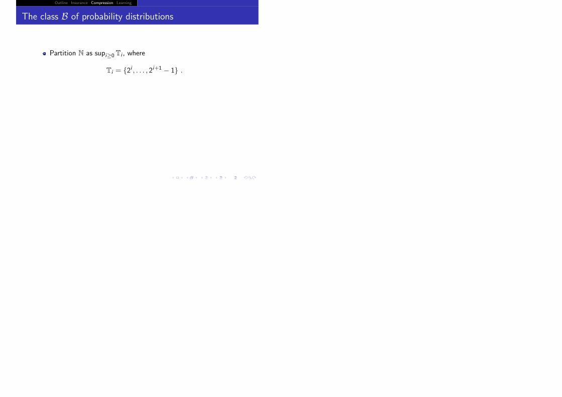
The class B of probability distributions
Partition N as supi≥0 Ti , where
Ti = {2i , . . . , 2i+1 − 1} .

Outline Insurance Compression Learning
The class B of probability distributions
Partition N as supi≥0 Ti , where
Ti = {2i , . . . , 2i+1 − 1} .
Given � > 0, let n� := �1� �, and for each 1 ≤ j ≤ 2n� , let p�,jbe the probability distribution assigning probability 1− � to T0
and � to the j-th smallest element of Tn� .
B is comprised of the p�,j and the distribution p0, whichassigns probability 1 to T0.
Then B is insurable, weakly compressible, but not d.w.c.

Outline Insurance Compression Learning
Outline
1 Insurance
2 Compression
3 Learning

Outline Insurance Compression Learning
PAC learning model

Outline Insurance Compression Learning
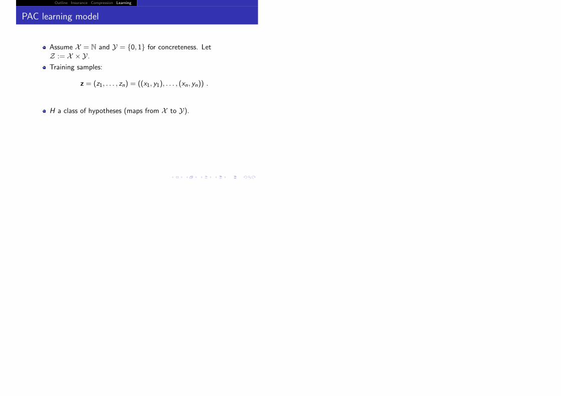
PAC learning model
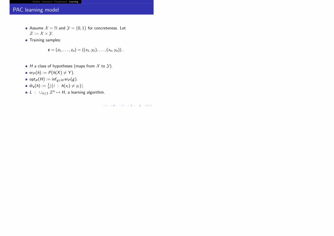
Assume X = N and Y = {0, 1} for concreteness. LetZ := X × Y.

Outline Insurance Compression Learning
PAC learning model
Assume X = N and Y = {0, 1} for concreteness. LetZ := X × Y.Training samples:
z = (z1, . . . , zn) = ((x1, y1), . . . , (xn, yn)) .
Outline Insurance Compression Learning
PAC learning model
Assume X = N and Y = {0, 1} for concreteness. LetZ := X × Y.Training samples:
z = (z1, . . . , zn) = ((x1, y1), . . . , (xn, yn)) .
H a class of hypotheses (maps from X to Y).

Outline Insurance Compression Learning
PAC learning model
Assume X = N and Y = {0, 1} for concreteness. LetZ := X × Y.Training samples:
z = (z1, . . . , zn) = ((x1, y1), . . . , (xn, yn)) .
H a class of hypotheses (maps from X to Y).erP(h) := P(h(X ) �= Y ).

Outline Insurance Compression Learning
PAC learning model
Assume X = N and Y = {0, 1} for concreteness. LetZ := X × Y.Training samples:
z = (z1, . . . , zn) = ((x1, y1), . . . , (xn, yn)) .
H a class of hypotheses (maps from X to Y).erP(h) := P(h(X ) �= Y ).
optP(H) := infg∈H erP(g).

Outline Insurance Compression Learning
PAC learning model
Assume X = N and Y = {0, 1} for concreteness. LetZ := X × Y.Training samples:
z = (z1, . . . , zn) = ((x1, y1), . . . , (xn, yn)) .
H a class of hypotheses (maps from X to Y).erP(h) := P(h(X ) �= Y ).
optP(H) := infg∈H erP(g).
erz(h) :=1n |{i : h(xi ) �= yi}|.
L : ∪n≥1 Zn �→ H, a learning algorithm.

Outline Insurance Compression Learning
PAC learning

Outline Insurance Compression Learning
PAC learning
Suppose that for all 0 < � < 1 and all 0 < δ < 1, there isn0(�, δ) ≥ 1, such that, for all n ≥ n0(�, δ) and all P we have
P(erP(L(Zn)) < optP(H) + �) ≥ 1− δ .
Then we say that the learning algorithm L PAC learns thehypothesis class H.

Outline Insurance Compression Learning
PAC learning
Suppose that for all 0 < � < 1 and all 0 < δ < 1, there isn0(�, δ) ≥ 1, such that, for all n ≥ n0(�, δ) and all P we have
P(erP(L(Zn)) < optP(H) + �) ≥ 1− δ .
Then we say that the learning algorithm L PAC learns thehypothesis class H.
Note the requirement for uniformity over the (i.i.d.)probability distribution driving the data.

Outline Insurance Compression Learning
VC dimension

Outline Insurance Compression Learning
VC dimension
The VC dimension of H is the supremum of the sizes ofsubsets of X shattered by H.

Outline Insurance Compression Learning
VC dimension
The VC dimension of H is the supremum of the sizes ofsubsets of X shattered by H.
There is a learning algorithm that learns H iff it has finite VCdimension. In fact, sample error minimization algorithms willthen learn H.

Outline Insurance Compression Learning
Data-derived pointwise PAC learning
Outline Insurance Compression Learning
Data-derived pointwise PAC learning
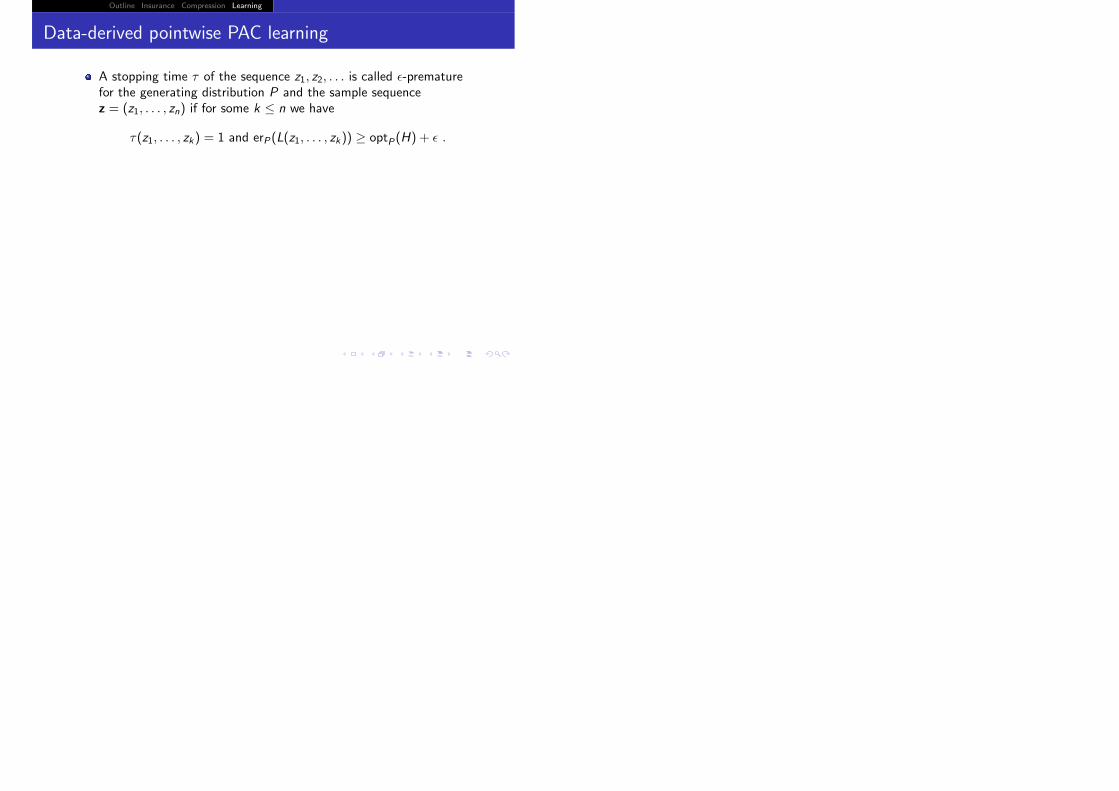
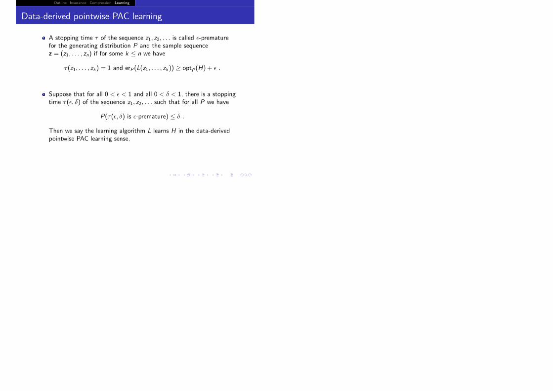
A stopping time τ of the sequence z1, z2, . . . is called �-prematurefor the generating distribution P and the sample sequencez = (z1, . . . , zn) if for some k ≤ n we have
τ(z1, . . . , zk) = 1 and erP(L(z1, . . . , zk)) ≥ optP(H) + � .
Outline Insurance Compression Learning
Data-derived pointwise PAC learning
A stopping time τ of the sequence z1, z2, . . . is called �-prematurefor the generating distribution P and the sample sequencez = (z1, . . . , zn) if for some k ≤ n we have
τ(z1, . . . , zk) = 1 and erP(L(z1, . . . , zk)) ≥ optP(H) + � .
Suppose that for all 0 < � < 1 and all 0 < δ < 1, there is a stoppingtime τ(�, δ) of the sequence z1, z2, . . . such that for all P we have
P(τ(�, δ) is �-premature) ≤ δ .
Then we say the learning algorithm L learns H in the data-derivedpointwise PAC learning sense.
Note that we have given the learning algorithm the opportunity todeclare that learning has taken place at a time that can depend onthe generating distribution (through the data itself).

Outline Insurance Compression Learning
The question of interest for PAC learning

Outline Insurance Compression Learning
The question of interest for PAC learning
For X = N and Y = {0, 1} as above, in fact the set of allhypotheses is data-derived pointwise PAC learnable.

Outline Insurance Compression Learning
The question of interest for PAC learning
For X = N and Y = {0, 1} as above, in fact the set of allhypotheses is data-derived pointwise PAC learnable.
This can be (vaguely) understood as coming from the“essential finiteness” of the support of each probabilitydistribution on N.

Outline Insurance Compression Learning
The question of interest for PAC learning
For X = N and Y = {0, 1} as above, in fact the set of allhypotheses is data-derived pointwise PAC learnable.
This can be (vaguely) understood as coming from the“essential finiteness” of the support of each probabilitydistribution on N.Question: Is data-derived pointwise PAC learnability of ahypothesis class characterized by finiteness of “local”complexity notions such as “local VC-dimension”, “localRademacher complexity”, “local Gaussian complexity”, etc.?

Outline Insurance Compression Learning
The End
Thank you!

Outline Insurance Compression Learning
Proof of sufficiency: preliminaries
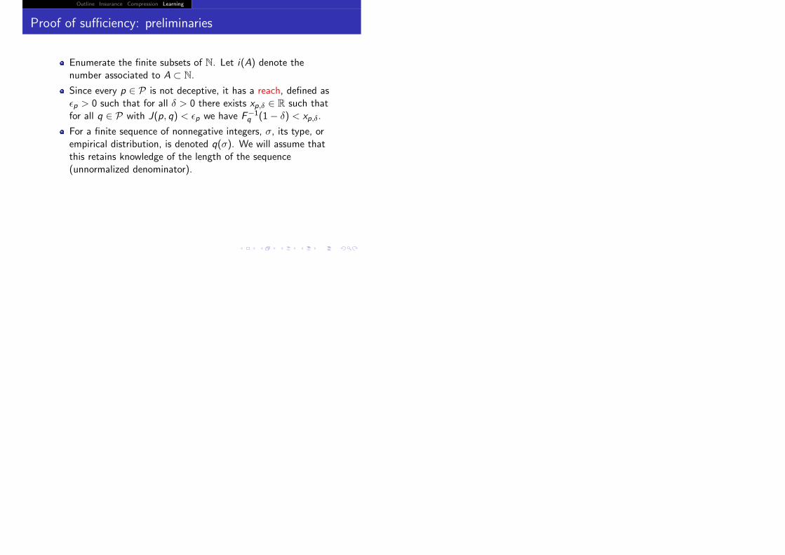
Enumerate the finite subsets of N. Let i(A) denote thenumber associated to A ⊂ N.

Outline Insurance Compression Learning
Proof of sufficiency: preliminaries
Enumerate the finite subsets of N. Let i(A) denote thenumber associated to A ⊂ N.Since every p ∈ P is not deceptive, it has a reach, defined as�p > 0 such that for all δ > 0 there exists xp,δ ∈ R such thatfor all q ∈ P with J(p, q) < �p we have F−1
q (1− δ) < xp,δ.
For a finite sequence of nonnegative integers, σ, its type, orempirical distribution, is denoted q(σ). We will assume thatthis retains knowledge of the length of the sequence(unnormalized denominator).
Given p, let
Ip := {q : |p − q|1 < �2p(ln 2)2
16} .

Outline Insurance Compression Learning
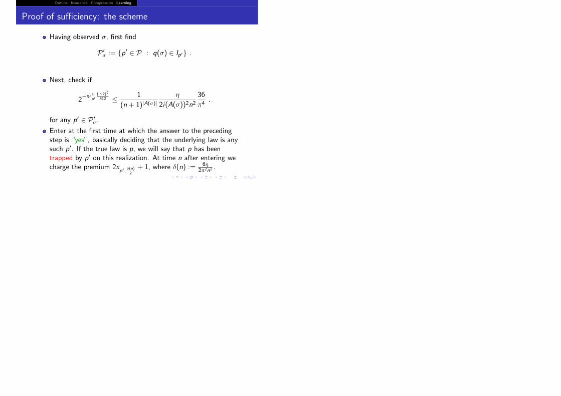
Proof of sufficiency: the scheme
Having observed σ, first find
P �σ := {p� ∈ P : q(σ) ∈ Ip�} .

Outline Insurance Compression Learning
Proof of sufficiency: the scheme
Having observed σ, first find
P �σ := {p� ∈ P : q(σ) ∈ Ip�} .
Next, check if
2−n�4
p�(ln 2)3
512 ≤ 1
(n + 1)|A(σ)|η
2i(A(σ))2n236
π4.
for any p� ∈ P �σ.
Outline Insurance Compression Learning
Proof of sufficiency: the scheme
Having observed σ, first find
P �σ := {p� ∈ P : q(σ) ∈ Ip�} .
Next, check if
2−n�4
p�(ln 2)3
512 ≤ 1
(n + 1)|A(σ)|η
2i(A(σ))2n236
π4.
for any p� ∈ P �σ.
Enter at the first time at which the answer to the precedingstep is “yes”, basically deciding that the underlying law is anysuch p�. If the true law is p, we will say that p has beentrapped by p� on this realization. At time n after entering wecharge the premium 2x
p�, δ(n)2
+ 1, where δ(n) := 6η2π2n2
.
Outline Insurance Compression Learning
Proof of sufficiency: entering with probability 1
Suppose the true loss distribution is p.
We will eventually have p ∈ P �σ (eventually in σ).
Since p is assumed to have finite alphabet, the empirical alphabeteventually stabilizes. Hence i(A(σ)) is eventually a constant. Thismeans the second criterion is also eventually met, so eventually theobserved sequence is trapped by some probability distribution in P.
Note: The only reason we need to assume finiteness of the range ofeach p ∈ P is because we need the empirical alphabet to stabilize.

Outline Insurance Compression Learning
Proof of sufficiency: Good traps
If the trapping p� is good, then at time n after being trapped, thepremium charged is 2x
p�, δ(n)2
+ 1, where δ(n) := 6η2π2n2
.
This is at least as big as 2F−1p (1− δ(n)
2 ) + 1.
So at time n after entering the loss bankrupts the scheme withprobability at most δ(n) := 6η
2π2n2.
Sum over n ≥ 1. The overall probability of going bankrupt overobserved loss sequences that get trapped in a good trap is at mostη2 ,
Outline Insurance Compression Learning
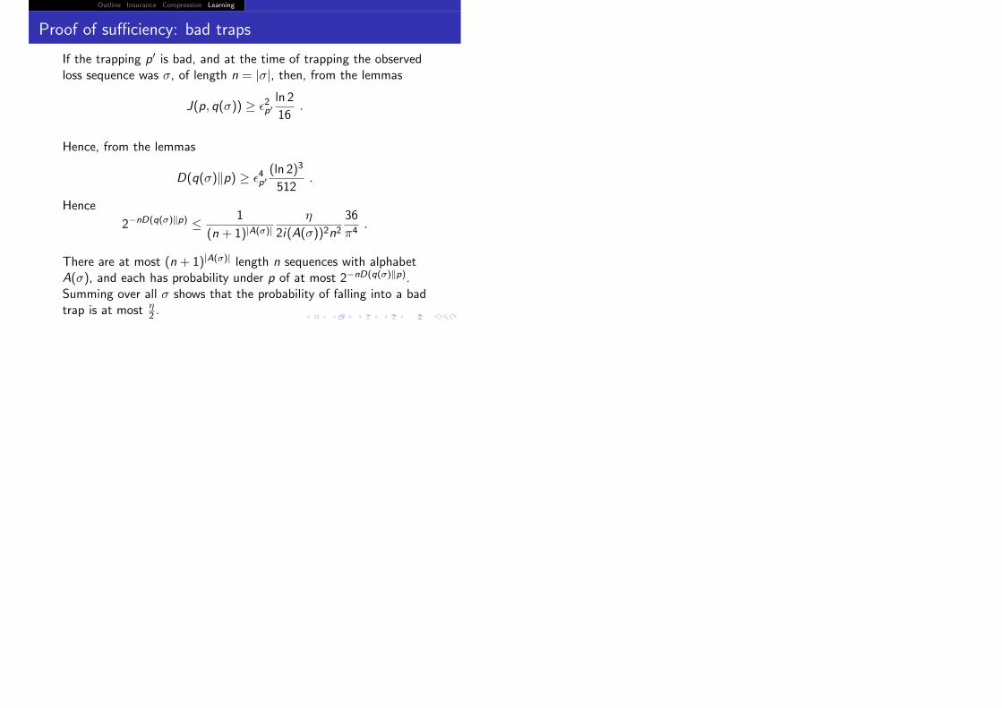
Proof of sufficiency: bad traps
If the trapping p� is bad, and at the time of trapping the observedloss sequence was σ, of length n = |σ|, then, from the lemmas
J(p, q(σ)) ≥ �2p�ln 2
16.
Hence, from the lemmas
D(q(σ)�p) ≥ �4p�(ln 2)3
512.
Hence
2−nD(q(σ)�p) ≤ 1
(n + 1)|A(σ)|η
2i(A(σ))2n236
π4.
There are at most (n + 1)|A(σ)| length n sequences with alphabetA(σ), and each has probability under p of at most 2−nD(q(σ)�p).Summing over all σ shows that the probability of falling into a badtrap is at most η
2 .

Outline Insurance Compression Learning
Proof of sufficiency without finite support assumption
The main observation is that P is Lindelof in the l1-topology,so the open covering of P by the sets
{Ip, p ∈ P}has a countable subcovering.
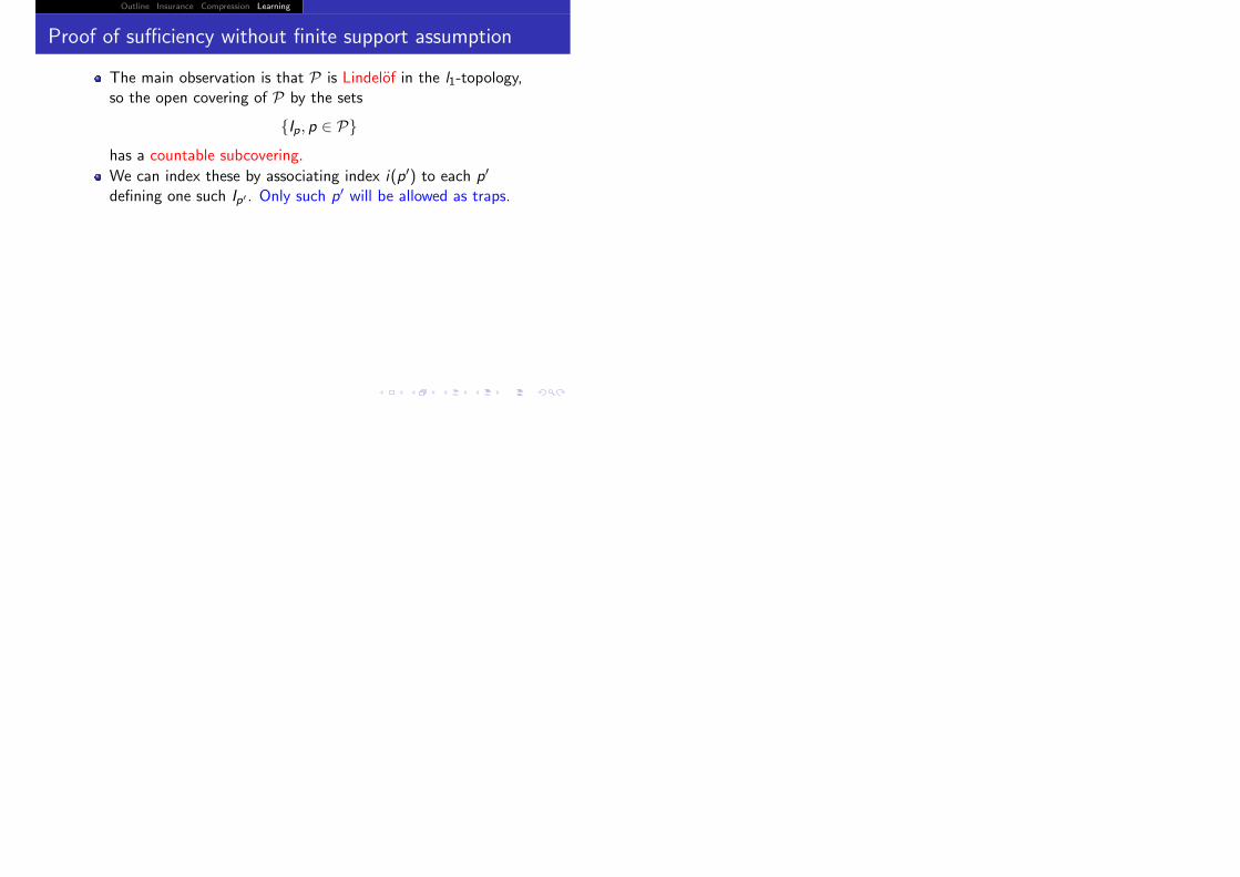
Outline Insurance Compression Learning
Proof of sufficiency without finite support assumption
The main observation is that P is Lindelof in the l1-topology,so the open covering of P by the sets
{Ip, p ∈ P}has a countable subcovering.
We can index these by associating index i(p�) to each p�
defining one such Ip� . Only such p� will be allowed as traps.
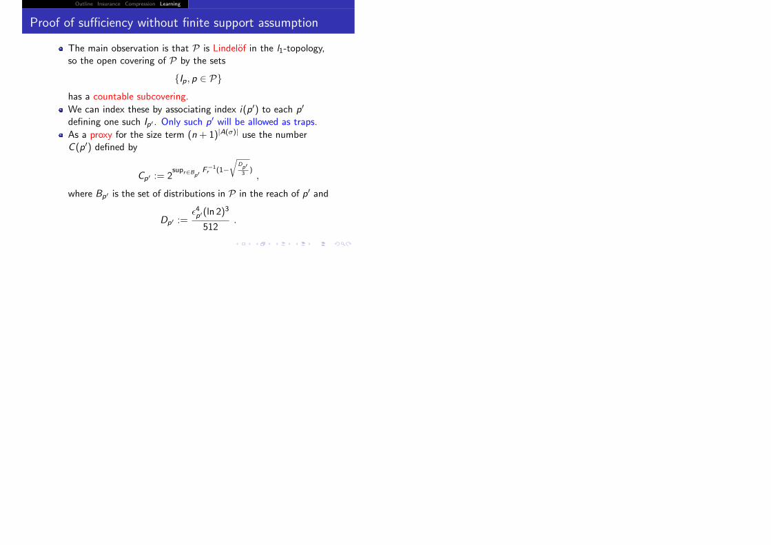
As a proxy for the size term (n + 1)|A(σ)| use the numberC (p�) defined by
Cp� := 2supr∈Bp�
F−1r (1−
�Dp�3
),
where Bp� is the set of distributions in P in the reach of p� and
Dp� :=�4p�(ln 2)
3
512.
The rest of the proof is the same.

Outline Insurance Compression Learning
Proof of necessity without finite support assumption
Hp,γ := {y ∈ Ap : y ≤ F−1p (1− γ
2)} ,
where Ap denotes the support of p, is called the head of p at levelγ.

Outline Insurance Compression Learning
Proof of necessity without finite support assumption
Hp,γ := {y ∈ Ap : y ≤ F−1p (1− γ
2)} ,
where Ap denotes the support of p, is called the head of p at levelγ.Let p ∈ P be deceptive. Given � > 0 and scheme Φ, for eachn ≥ 1 let:
Rn := {xn : Φ(xn) < ∞} ,
as before.

Outline Insurance Compression Learning
Proof of necessity without finite support assumption
Hp,γ := {y ∈ Ap : y ≤ F−1p (1− γ
2)} ,
where Ap denotes the support of p, is called the head of p at levelγ.Let p ∈ P be deceptive. Given � > 0 and scheme Φ, for eachn ≥ 1 let:
Rn := {xn : Φ(xn) < ∞} ,
as before.Now, pick N ≥ 1 such that
p(RN) > 1− α
2,
where α < 1− ln 2 as in the lemma. Later N → ∞.

Outline Insurance Compression Learning
Proof of necessity without finite support assumption
Hp,γ := {y ∈ Ap : y ≤ F−1p (1− γ
2)} ,
where Ap denotes the support of p, is called the head of p at levelγ.Let p ∈ P be deceptive. Given � > 0 and scheme Φ, for eachn ≥ 1 let:
Rn := {xn : Φ(xn) < ∞} ,
as before.Now, pick N ≥ 1 such that
p(RN) > 1− α
2,
where α < 1− ln 2 as in the lemma. Later N → ∞.Let
Rp,γ,i := {x i ∈ Ri : A(x i ) ⊆ Hp,γ , entered by N} ,
where A(xn) denotes the set of values showing up in xn.

Outline Insurance Compression Learning
Proof of necessity without finite support assumption
Pick k ≥ 2 (depending on δ) such that
(1− 1
Nk)N+� 1
δ� ≥ 1− α
2.
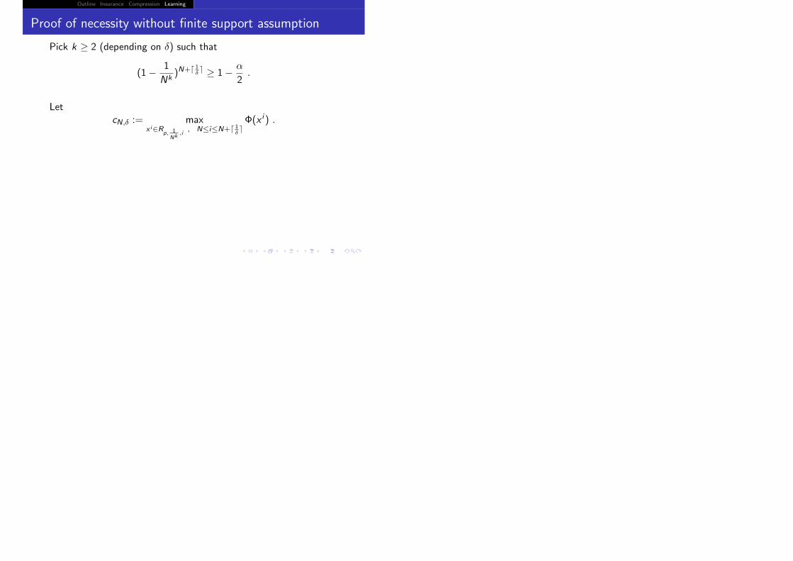
Outline Insurance Compression Learning
Proof of necessity without finite support assumption
Pick k ≥ 2 (depending on δ) such that
(1− 1
Nk)N+� 1
δ� ≥ 1− α
2.
LetcN,δ := max
xi∈Rp, 1
Nk,i
, N≤i≤N+� 1δ�Φ(x i ) .
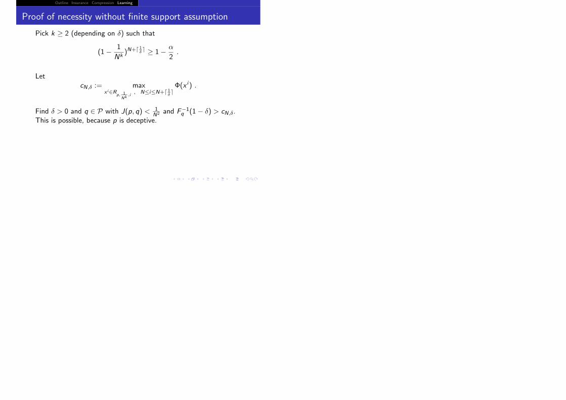
Outline Insurance Compression Learning
Proof of necessity without finite support assumption
Pick k ≥ 2 (depending on δ) such that
(1− 1
Nk)N+� 1
δ� ≥ 1− α
2.
LetcN,δ := max
xi∈Rp, 1
Nk,i
, N≤i≤N+� 1δ�Φ(x i ) .
Find δ > 0 and q ∈ P with J(p, q) < 1N2 and F−1
q (1− δ) > cN,δ.This is possible, because p is deceptive.

Outline Insurance Compression Learning
Proof of necessity without finite support assumption
Pick k ≥ 2 (depending on δ) such that
(1− 1
Nk)N+� 1
δ� ≥ 1− α
2.
LetcN,δ := max
xi∈Rp, 1
Nk,i
, N≤i≤N+� 1δ�Φ(x i ) .
Find δ > 0 and q ∈ P with J(p, q) < 1N2 and F−1
q (1− δ) > cN,δ.This is possible, because p is deceptive.Then, for all N ≤ i ≤ N + �1δ �, we have
q(Rp, 1
Nk ,i) ≥ 1− 2
N− 2h(α) ,
for all N ≤ i ≤ N + �1δ �, by the lemma.
Outline Insurance Compression Learning
Proof of necessity without finite support assumption
Pick k ≥ 2 (depending on δ) such that
(1− 1
Nk)N+� 1
δ� ≥ 1− α
2.
LetcN,δ := max
xi∈Rp, 1
Nk,i
, N≤i≤N+� 1δ�Φ(x i ) .
Find δ > 0 and q ∈ P with J(p, q) < 1N2 and F−1
q (1− δ) > cN,δ.This is possible, because p is deceptive.Then, for all N ≤ i ≤ N + �1δ �, we have
q(Rp, 1
Nk ,i) ≥ 1− 2
N− 2h(α) ,
for all N ≤ i ≤ N + �1δ �, by the lemma.The rest of the proof is as before.