data communication and computer networking (dccn)

DEPARTMENT OF

ELECTRONICS AND COMMUNICATION ENGINEERING

LECTURE NOTES

ON

DATA COMMUNICATION AND COMPUTERNETWORKING (DCCN)

B.E VI Semester (PE672 EC)

Mr. I. SRIKANTH,Associate ProfessorDepartment of ECE

2019-2020

UNIT-1

Specific Instructional Objective

On Completion of this lesson, the students will be able to:

• Define Computer Networks • State the evolution of Computer Networks • Categorize different types of Computer Networks • Specify some of the application of Computer Networks

1.1.1 Introduction

The concept of Network is not new. In simple terms it means an interconnected set of some objects. For decades we are familiar with the Radio, Television, railway, Highway, Bank and other types of networks. In recent years, the network that is making significant impact in our day-to-day life is the Computer network. By computer network we mean an interconnected set of autonomous computers. The term autonomous implies that the computers can function independent of others. However, these computers can exchange information with each other through the communication network system. Computer networks have emerged as a result of the convergence of two technologies of this century- Computer and Communication as shown in Fig. 1.1.1. The consequence of this revolutionary merger is the emergence of a integrated system that transmit all types of data and information. There is no fundamental difference between data communications and data processing and there are no fundamental differences among data, voice and video communications. After a brief historical background in Section 1.1.2, Section 1.1.2 introduces different network categories. A brief overview of the applications of computer networks is presented in Section 1.1.3. Finally an outline of the entire course is given in Section 1.1.4.

Figure 1.1.1 Evolution of computer networks

Version 2 CSE IIT, Kharagpur

1.1.2 Historical Background The history of electronic computers is not very old. It came into existence in the early 1950s and during the first two decades of its existence it remained as a centralized system housed in a single large room. In those days the computers were large in size and were operated by trained personnel. To the users it was a remote and mysterious object having no direct communication with the users. Jobs were submitted in the form of punched cards or paper tape and outputs were collected in the form of computer printouts. The submitted jobs were executed by the computer one after the other, which is referred to as batch mode of data processing. In this scenario, there was long delay between the submission of jobs and receipt of the results. In the 1960s, computer systems were still centralize, but users provided with direct access through interactive terminals connected by point-to-point low-speed data links with the computer. In this situation, a large number of users, some of them located in remote locations could simultaneously access the centralized computer in time-division multiplexed mode. The users could now get immediate interactive feedback from the computer and correct errors immediately. Following the introduction of on-line terminals and time-sharing operating systems, remote terminals were used to use the central computer. With the advancement of VLSI technology, and particularly, after the invention of microprocessors in the early 1970s, the computers became smaller in size and less expensive, but with significant increase in processing power. New breed of low-cost computers known as mini and personal computers were introduced. Instead of having a single central computer, an organization could now afford to own a number of computers located in different departments and sections. Side-by-side, riding on the same VLSI technology the communication technology also advanced leading to the worldwide deployment of telephone network, developed primarily for voice communication. An organization having computers located geographically dispersed locations wanted to have data communications for diverse applications. Communication was required among the machines of the same kind for collaboration, for the use of common software or data or for sharing of some costly resources. This led to the development of computer networks by successful integration and cross-fertilization of communications and geographically dispersed computing facilities. One significant development was the APPANET (Advanced Research Projects Agency Network). Starting with four-node experimental network in 1969, it has subsequently grown into a network several thousand computers spanning half of the globe, from Hawaii to Sweden. Most of the present-day concepts such as packet switching evolved from the ARPANET project. The low bandwidth (3KHz on a voice grade line) telephone network was the only generally available communication system available for this type of network.


The bandwidth was clearly a problem, and in the late 1970s and early 80s another new communication technique known as Local Area Networks (LANs) evolved, which helped computers to communicate at high speed over a small geographical area. In the later years use of optical fiber and satellite communication allowed high-speed data communications over long distances. 1.1.3 Network Technologies

There is no generally accepted taxonomy into which all computer networks fit, but two dimensions stand out as important: Transmission Technology and Scale. The classifications based on these two basic approaches are considered in this section.

1.1.3.1 Classification Based on Transmission Technology

Computer networks can be broadly categorized into two types based on transmission technologies:

• Broadcast networks • Point-to-point networks

1.2.3.1.1 Broadcast Networks

Broadcast network have a single communication channel that is shared by all the machines on the network as shown in Figs.1.1.2 and 1.1.3. All the machines on the network receive short messages, called packets in certain contexts, sent by any machine. An address field within the packet specifies the intended recipient. Upon receiving a packet, machine checks the address field. If packet is intended for itself, it processes the packet; if packet is not intended for itself it is simply ignored.

Figure 1.1.2 Example of a broadcast network based on shared bus


Figure 1.1.3 Example of a broadcast network based on satellite communication

This system generally also allows possibility of addressing the packet to all destinations (all nodes on the network). When such a packet is transmitted and received by all the machines on the network. This mode of operation is known as Broadcast Mode. Some Broadcast systems also supports transmission to a sub-set of machines, something known as Multicasting.

1.2.3.1.2 Point-to-Point Networks

A network based on point-to-point communication is shown in Fig. 1.1.4. The end devices that wish to communicate are called stations. The switching devices are called nodes. Some Nodes connect to other nodes and some to attached stations. It uses FDM or TDM for node-to-node communication. There may exist multiple paths between a source-destination pair for better network reliability. The switching nodes are not concerned with the contents of data. Their purpose is to provide a switching facility that will move data from node to node until they reach the destination.


Figure 1.1.4 Communication network based on point-to-point communication

As a general rule (although there are many exceptions), smaller, geographically localized networks tend to use broadcasting, whereas larger networks normally use are point-to-point communication.

1.1.3.2 Classification based on Scale

Alternative criteria for classifying networks are their scale. They are divided into Local Area (LAN), Metropolitan Area Network (MAN) and Wide Area Networks (WAN).

1.1.3.2.1 Local Area Network (LAN)

LAN is usually privately owned and links the devices in a single office, building or campus of up to few kilometers in size. These are used to share resources (may be hardware or software resources) and to exchange information. LANs are distinguished from other kinds of networks by three categories: their size, transmission technology and topology.

LANs are restricted in size, which means that their worst-case transmission time is bounded and known in advance. Hence this is more reliable as compared to MAN and WAN. Knowing this bound makes it possible to use certain kinds of design that would not otherwise be possible. It also simplifies network management.


Figure 1.1.5 Local Area Network

LAN typically used transmission technology consisting of single cable to which all machines are connected. Traditional LANs run at speeds of 10 to 100 Mbps (but now much higher speeds can be achieved). The most common LAN topologies are bus, ring and star. A typical LAN is shown in Fig. 1.1.5.


1.1.3.2.2 Metropolitan Area Networks (MAN)

MAN is designed to extend over the entire city. It may be a single network as a cable TV network or it may be means of connecting a number of LANs into a larger network so that resources may be shared as shown in Fig. 1.1.6. For example, a company can use a MAN to connect the LANs in all its offices in a city. MAN is wholly owned and operated by a private company or may be a service provided by a public company.

Figure 1.1.6 Metropolitan Area Networks (MAN)

The main reason for distinguishing MANs as a special category is that a standard has been adopted for them. It is DQDB (Distributed Queue Dual Bus) or IEEE 802.6.

1.1.3.2.3 Wide Area Network (WAN)

WAN provides long-distance transmission of data, voice, image and information over large geographical areas that may comprise a country, continent or even the whole world. In contrast to LANs, WANs may utilize public, leased or private communication devices, usually in combinations, and can therefore span an unlimited number of miles as shown


in Fig. 1.1.7. A WAN that is wholly owned and used by a single company is often referred to as enterprise network.

Figure 1.1.7 Wide Area Network

1.1.3.2.4 The Internet

Internet is a collection of networks or network of networks. Various networks such as LAN and WAN connected through suitable hardware and software to work in a seamless manner. Schematic diagram of the Internet is shown in Fig. 1.1.8. It allows various applications such as e-mail, file transfer, remote log-in, World Wide Web, Multimedia, etc run across the internet. The basic difference between WAN and Internet is that WAN is owned by a single organization while internet is not so. But with the time the line between WAN and Internet is shrinking, and these terms are sometimes used interchangeably.


Figure 1.1.8 Internet – network of networks

1.1.4 Applications

In a short period of time computer networks have become an indispensable part of business, industry, entertainment as well as a common-man's life. These applications have changed tremendously from time and the motivation for building these networks are all essentially economic and technological.

Initially, computer network was developed for defense purpose, to have a secure communication network that can even withstand a nuclear attack. After a decade or so, companies, in various fields, started using computer networks for keeping track of inventories, monitor productivity, communication between their different branch offices located at different locations. For example, Railways started using computer networks by connecting their nationwide reservation counters to provide the facility of reservation and enquiry from any where across the country.

And now after almost two decades, computer networks have entered a new dimension; they are now an integral part of the society and people. In 1990s, computer network started delivering services to private individuals at home. These services and motivation for using them are quite different. Some of the services are access to remote information, person-person communication, and interactive entertainment. So, some of the applications of computer networks that we can see around us today are as follows:

Marketing and sales: Computer networks are used extensively in both marketing and sales organizations. Marketing professionals use them to collect, exchange, and analyze data related to customer needs and product development cycles. Sales application


includes teleshopping, which uses order-entry computers or telephones connected to order processing network, and online-reservation services for hotels, airlines and so on.

Financial services: Today's financial services are totally depended on computer networks. Application includes credit history searches, foreign exchange and investment services, and electronic fund transfer, which allow user to transfer money without going into a bank (an automated teller machine is an example of electronic fund transfer, automatic pay-check is another).

Manufacturing: Computer networks are used in many aspects of manufacturing including manufacturing process itself. Two of them that use network to provide essential services are computer-aided design (CAD) and computer-assisted manufacturing (CAM), both of which allow multiple users to work on a project simultaneously.

Directory services: Directory services allow list of files to be stored in central location to speed worldwide search operations.

Information services: A Network information service includes bulletin boards and data banks. A World Wide Web site offering technical specification for a new product is an information service.

Electronic data interchange (EDI): EDI allows business information, including documents such as purchase orders and invoices, to be transferred without using paper.

Electronic mail: probably it's the most widely used computer network application.

Teleconferencing: Teleconferencing allows conference to occur without the participants being in the same place. Applications include simple text conferencing (where participants communicate through their normal keyboards and monitor) and video conferencing where participants can even see as well as talk to other fellow participants. Different types of equipments are used for video conferencing depending on what quality of the motion you want to capture (whether you want just to see the face of other fellow participants or do you want to see the exact facial expression).

Voice over IP: Computer networks are also used to provide voice communication. This kind of voice communication is pretty cheap as compared to the normal telephonic conversation.

Video on demand: Future services provided by the cable television networks may include video on request where a person can request for a particular movie or any clip at anytime he wish to see.

Summary: The main area of applications can be broadly classified into following categories:


Specific Functional Objectives On Completion of this lesson, the students will be able to:

• State the requirement for layered approach • Explain the basic concept of layering in the network model • Define entities protocols in networking context • Describe ISO’s OSI Reference Model • Explain information flow in OSI references Model. • Explain functions of the seven layers of OSI Model

1.2.1 Basic concept of layering

Network architectures define the standards and techniques for designing and building communication systems for computers and other devices. In the past, vendors developed their own architectures and required that other vendors conform to this architecture if they wanted to develop compatible hardware and software. There are proprietary network architectures such as IBM's SNA (Systems Network Architecture) and there are open architectures like the OSI (Open Systems Interconnection) model defined by the International Organization for Standardization. The previous strategy, where the computer network is designed with the hardware as the main concern and software is afterthought, no longer works. Network software is now highly structured.

To reduce the design complexity, most of the networks are organized as a series of layers or levels, each one build upon one below it. The basic idea of a layered architecture is to divide the design into small pieces. Each layer adds to the services provided by the lower layers in such a manner that the highest layer is provided a full set of services to manage communications and run the applications. The benefits of the layered models are modularity and clear interfaces, i.e. open architecture and comparability between the different providers' components.

A basic principle is to ensure independence of layers by defining services provided by each layer to the next higher layer without defining how the services are to be performed. This permits changes in a layer without affecting other layers. Prior to the use of layered protocol architectures, simple changes such as adding one terminal type to the list of those supported by an architecture often required changes to essentially all communications software at a site. The number of layers, functions and contents of each layer differ from network to network. However in all networks, the purpose of each layer is to offer certain services to higher layers, shielding those layers from the details of how the services are actually implemented.

The basic elements of a layered model are services, protocols and interfaces. A service is a set of actions that a layer offers to another (higher) layer. Protocol is a set of rules that a layer uses to exchange information with a peer entity. These rules concern both the contents and the order of the messages used. Between the layers service interfaces are defined. The messages from one layer to another are sent through those interfaces.


In an n-layer architecture, layer n on one machine carries on conversation with the layer n on other machine. The rules and conventions used in this conversation are collectively known as the layer-n protocol. Basically, a protocol is an agreement between the communicating parties on how communication is to proceed. Violating the protocol will make communication more difficult, if not impossible. A five-layer architecture is shown in Fig. 1.2.1, the entities comprising the corresponding layers on different machines are called peers. In other words, it is the peers that communicate using protocols. In reality, no data is transferred from layer n on one machine to layer n of another machine. Instead, each layer passes data and control information to the layer immediately below it, until the lowest layer is reached. Below layer-1 is the physical layer through which actual communication occurs. The peer process abstraction is crucial to all network design. Using it, the un-manageable tasks of designing the complete network can be broken into several smaller, manageable, design problems, namely design of individual layers.

Figure 1.2.1 Basic five layer architecture

Between each pair of adjacent layers there is an interface. The interface defines which primitives operations and services the lower layer offers to the upper layer adjacent to it. When network designer decides how many layers to include in the network and what each layer should do, one of the main considerations is defining clean interfaces between adjacent layers. Doing so, in turns requires that each layer should perform well-defined functions. In addition to minimize the amount of information passed between layers, clean-cut interface also makes it simpler to replace the implementation of one layer with a completely different implementation, because all what is required of new implementation is that it offers same set of services to its upstairs neighbor as the old implementation (that is what a layer provides and how to use that service from it is more important than knowing how exactly it implements it).


A set of layers and protocols is known as network architecture. The specification of architecture must contain enough information to allow an implementation to write the program or build the hardware for each layer so that it will correctly obey the appropriate protocol. Neither the details of implementation nor the specification of interface is a part of network architecture because these are hidden away inside machines and not visible from outside. It is not even necessary that the interface on all machines in a network be same, provided that each machine can correctly use all protocols. A list of protocols used by a certain system, one protocol per layer, is called protocol stack.

Summary: Why Layered architecture?

1. To make the design process easy by breaking unmanageable tasks into several smaller and manageable tasks (by divide-and-conquer approach).

2. Modularity and clear interfaces, so as to provide comparability between the different providers' components.

3. Ensure independence of layers, so that implementation of each layer can be changed or modified without affecting other layers.

4. Each layer can be analyzed and tested independently of all other layers.

1.2.2 Open System Interconnection Reference Model The Open System Interconnection (OSI) reference model describes how information from a software application in one computer moves through a network medium to a software application in another computer. The OSI reference model is a conceptual model composed of seven layers, each specifying particular network functions. The model was developed by the International Organization for Standardization (ISO) in 1984, and it is now considered the primary architectural model for inter-computer communications. The OSI model divides the tasks involved with moving information between networked computers into seven smaller, more manageable task groups. A task or group of tasks is then assigned to each of the seven OSI layers. Each layer is reasonably self-contained so that the tasks assigned to each layer can be implemented independently. This enables the solutions offered by one layer to be updated without adversely affecting the other layers.

The OSI Reference Model includes seven layers:

7. Application Layer: Provides Applications with access to network services.

6. Presentation Layer: Determines the format used to exchange data among networked computers.


5. Session Layer: Allows two applications to establish, use and disconnect a connection between them called a session. Provides for name recognition and additional functions like security, which are needed to allow applications to communicate over the network.

4. Transport Layer: Ensures that data is delivered error free, in sequence and with no loss, duplications or corruption. This layer also repackages data by assembling long messages into lots of smaller messages for sending, and repackaging the smaller messages into the original larger message at the receiving end.

3. Network Layer: This is responsible for addressing messages and data so they are sent to the correct destination, and for translating logical addresses and names (like a machine name FLAME) into physical addresses. This layer is also responsible for finding a path through the network to the destination computer.

2. Data-Link Layer: This layer takes the data frames or messages from the Network Layer and provides for their actual transmission. At the receiving computer, this layer receives the incoming data and sends it to the network layer for handling. The Data-Link Layer also provides error-free delivery of data between the two computers by using the physical layer. It does this by packaging the data from the Network Layer into a frame, which includes error detection information. At the receiving computer, the Data-Link Layer reads the incoming frame, and generates its own error detection information based on the received frames data. After receiving the entire frame, it then compares its error detection value with that of the incoming frames, and if they match, the frame has been received correctly.

1. Physical Layer: Controls the transmission of the actual data onto the network cable. It defines the electrical signals, line states and encoding of the data and the connector types used. An example is 10BaseT.

1.2.2.1Characteristics of the OSI Layers

The seven layers of the OSI reference model can be divided into two categories: upper layers and lower layers as shown in Fig. 1.2.2.

The upper layers of the OSI model deal with application issues and generally are implemented only in software. The highest layer, the application layer, is closest to the end user. Both users and application layer processes interact with software applications that contain a communications component. The term upper layer is sometimes used to refer to any layer above another layer in the OSI model.

The lower layers of the OSI model handle data transport issues. The physical layer and the data link layer are implemented in hardware and software. The lowest layer, the physical layer, is closest to the physical network medium (the network cabling, for example) and is responsible for actually placing information on the medium .


Figure 1.2.2 Two sets of layers make up the OSI layers

1.2.2.2 Protocols

The OSI model provides a conceptual framework for communication between computers, but the model itself is not a method of communication. Actual communication is made possible by using communication protocols. In the context of data networking, a protocol is a formal set of rules and conventions that governs how computers exchange information over a network medium. A protocol implements the functions of one or more of the OSI layers.

A wide variety of communication protocols exist. Some of these protocols include LAN protocols, WAN protocols, network protocols, and routing protocols. LAN protocols operate at the physical and data link layers of the OSI model and define communication over various LAN media. WAN protocols operate at the lowest three layers of the OSI model and define communication over the various wide-area media. Routing protocols are network layer protocols that are responsible for exchanging information between routers so that the routers can select the proper path for network traffic. Finally, network protocols are the various upper-layer protocols that exist in a given protocol suite. Many protocols rely on others for operation. For example, many routing protocols use network


protocols to exchange information between routers. This concept of building upon the layers already in existence is the foundation of the OSI model.

1.2.2.3 OSI Model and Communication between Systems

Information being transferred from a software application in one computer system to a software application in another must pass through the OSI layers. For example, if a software application in System A has information to transmit to a software application in System B, the application program in System A will pass its information to the application layer (Layer 7) of System A. The application layer then passes the information to the presentation layer (Layer 6), which relays the data to the session layer (Layer 5), and so on down to the physical layer (Layer 1). At the physical layer, the information is placed on the physical network medium and is sent across the medium to System B. The physical layer of System B removes the information from the physical medium, and then its physical layer passes the information up to the data link layer (Layer 2), which passes it to the network layer (Layer 3), and so on, until it reaches the application layer (Layer 7) of System B. Finally, the application layer of System B passes the information to the recipient application program to complete the communication process.

1.2.2.4 Interaction between OSI Model Layers

A given layer in the OSI model generally communicates with three other OSI layers: the layer directly above it, the layer directly below it, and its peer layer in other networked computer systems. The data link layer in System A, for example, communicates with the network layer of System A, the physical layer of System A, and the data link layer in System B. Figure1.2.3 illustrates this example.

Figure 1.2.3 OSI Model Layers Communicate with Other Layers


1.2.3 Services and service access points

One OSI layer communicates with another layer to make use of the services provided by the second layer. The services provided by adjacent layers help a given OSI layer communicate with its peer layer in other computer systems. Three basic elements are involved in layer services: the service user, the service provider, and the service access point (SAP).

In this context, the service user is the OSI layer that requests services from an adjacent OSI layer. The service provider is the OSI layer that provides services to service users. OSI layers can provide services to multiple service users. The SAP is a conceptual location at which one OSI layer can request the services of another OSI layer.

Figure 1.2.4 Service Users, Providers, and SAPs interact at the Network and Data Link Layers

1.2.3.1 OSI Model Layers and Information Exchange

The seven OSI layers use various forms of control information to communicate with their peer layers in other computer systems. This control information consists of specific requests and instructions that are exchanged between peer OSI layers.

Control information typically takes one of two forms: headers and trailers. Headers are prepended to data that has been passed down from upper layers. Trailers are appended to data that has been passed down from upper layers. An OSI layer is not required to attach a header or a trailer to data from upper layers.

Headers, trailers, and data are relative concepts, depending on the layer that analyzes the information unit. At the network layer, for example, an information unit consists of a


Layer 3 header and data. At the data link layer, however, all the information passed down by the network layer (the Layer 3 header and the data) is treated as data.

In other words, the data portion of an information unit at a given OSI layer potentially can contain headers, trailers, and data from all the higher layers. This is known as encapsulation. Figure 1-6 shows how the header and data from one layer are encapsulated into the header of the next lowest layer.

Figure 1.2.6 Headers and Data can be encapsulated during Information exchange

1.2.3.2 Information Exchange Process

The information exchange process occurs between peer OSI layers. Each layer in the source system adds control information to data, and each layer in the destination system analyzes and removes the control information from that data.

If system A has data from software application to send to System B, the data is passed to the application layer. The application layer in System A then communicates any control information required by the application layer in System B by pre-pending a header to the data. The resulting information unit (a header and the data) is passed to the presentation layer, which pre-pends its own header containing control information intended for the presentation layer in System B. The information unit grows in size as each layer pre-pends its own header (and, in some cases, a trailer) that contains control information to be


used by its peer layer in System B. At the physical layer, the entire information unit is placed onto the network medium.

The physical layer in System B receives the information unit and passes it to the data link layer. The data link layer in System B then reads the control information contained in the header pre-pended by the data link layer in System A. The header is then removed, and the remainder of the information unit is passed to the network layer. Each layer performs the same actions: The layer reads the header from its peer layer, strips it off, and passes the remaining information unit to the next highest layer. After the application layer performs these actions, the data is passed to the recipient software application in System B, in exactly the form in which it was transmitted by the application in System A.

1.2.4 Functions of the OSI Layers

Functions of different layers of the OSI model are presented in this section.

1.2.4.1 Physical Layer

The physical layer is concerned with transmission of raw bits over a communication channel. It specifies the mechanical, electrical and procedural network interface specifications and the physical transmission of bit streams over a transmission medium connecting two pieces of communication equipment. In simple terns, the physical layer decides the following:

• Number of pins and functions of each pin of the network connector (Mechanical) • Signal Level, Data rate (Electrical) • Whether simultaneous transmission in both directions • Establishing and breaking of connection • Deals with physical transmission

There exist a variety of physical layer protocols such as RS-232C, Rs-449 standards developed by Electronics Industries Association (EIA).

1.2.4.2 Data Link Layer

The goal of the data link layer is to provide reliable, efficient communication between adjacent machines connected by a single communication channel. Specifically:

1. Group the physical layer bit stream into units called frames. Note that frames are nothing more than ``packets'' or ``messages''. By convention, we shall use the term ``frames'' when discussing DLL packets.

2. Sender calculates the checksum and sends checksum together with data. The checksum allows the receiver to determine when a frame has been damaged in transit or received correctly.


3. Receiver recomputes the checksum and compares it with the received value. If they differ, an error has occurred and the frame is discarded.

4. Error control protocol returns a positive or negative acknowledgment to the sender. A positive acknowledgment indicates the frame was received without errors, while a negative acknowledgment indicates the opposite.

5. Flow control prevents a fast sender from overwhelming a slower receiver. For example, a supercomputer can easily generate data faster than a PC can consume it.

6. In general, data link layer provides service to the network layer. The network layer wants to be able to send packets to its neighbors without worrying about the details of getting it there in one piece.

1.2.4.2.1 Design Issues Below are the some of the important design issues of the data link layer:

a). Reliable Delivery:

Frames are delivered to the receiver reliably and in the same order as generated by the sender. Connection state keeps track of sending order and which frames require retransmission. For example, receiver state includes which frames have been received, which ones have not, etc.

b). Best Effort: The receiver does not return acknowledgments to the sender, so the sender has no way of knowing if a frame has been successfully delivered.

When would such a service be appropriate?

1. When higher layers can recover from errors with little loss in performance. That is, when errors are so infrequent that there is little to be gained by the data link layer performing the recovery. It is just as easy to have higher layers deal with occasional loss of packet.

2. For real-time applications requiring ``better never than late'' semantics. Old data may be worse than no data.

c). Acknowledged Delivery The receiver returns an acknowledgment frame to the sender indicating that a data frame was properly received. This sits somewhere between the other two in that the sender keeps connection state, but may not necessarily retransmit unacknowledged frames. Likewise, the receiver may hand over received packets to higher layer in the order in


which they arrive, regardless of the original sending order. Typically, each frame is assigned a unique sequence number, which the receiver returns in an acknowledgment frame to indicate which frame the ACK refers to. The sender must retransmit unacknowledged (e.g., lost or damaged) frames.

d). Framing

The DLL translates the physical layer's raw bit stream into discrete units (messages) called frames. How can the receiver detect frame boundaries? Various techniques are used for this: Length Count, Bit Stuffing, and Character stuffing.

e). Error Control

Error control is concerned with insuring that all frames are eventually delivered (possibly in order) to a destination. To achieve this, three items are required: Acknowledgements, Timers, and Sequence Numbers.

f). Flow Control

Flow control deals with throttling the speed of the sender to match that of the receiver. Usually, this is a dynamic process, as the receiving speed depends on such changing factors as the load, and availability of buffer space.

1.2.4.2.2 Link Management In some cases, the data link layer service must be ``opened'' before use:

• The data link layer uses open operations for allocating buffer space, control blocks, agreeing on the maximum message size, etc.

• Synchronize and initialize send and receive sequence numbers with its peer at the other end of the communications channel.

1.2.4.2.3 Error Detection and Correction

In data communication, error may occur because of various reasons including attenuation, noise. Moreover, error usually occurs as bursts rather than independent, single bit errors. For example, a burst of lightning will affect a set of bits for a short time after the lightning strike. Detecting and correcting errors requires redundancy (i.e., sending additional information along with the data).

There are two types of attacks against errors:

• Error Detecting Codes: Include enough redundancy bits to detect errors and use ACKs and retransmissions to recover from the errors. Example: parity encoding.

• Error Correcting Codes: Include enough redundancy to detect and correct errors. Examples: CRC checksum, MD5.


1.2.4.3 Network Layer

The basic purpose of the network layer is to provide an end-to-end communication capability in contrast to machine-to-machine communication provided by the data link layer. This end-to-end is performed using two basic approaches known as connection-oriented or connectionless network-layer services.

1.2.4.3.1 Four issues:

1. Interface between the host and the network (the network layer is typically the boundary between the host and subnet)

2. Routing

3. Congestion and deadlock

4. Internetworking (A path may traverse different network technologies (e.g., Ethernet, point-to-point links, etc.)

1.2.4.3.2 Network Layer Interface

There are two basic approaches used for sending packets, which is a group of bits that includes data plus source and destination addresses, from node to node called virtual circuit and datagram methods. These are also referred to as connection-oriented and connectionless network-layer services. In virtual circuit approach, a route, which consists of logical connection, is first established between two users. During this establishment phase, the two users not only agree to set up a connection between them but also decide upon the quality of service to be associated with the connection. The well-known virtual-circuit protocol is the ISO and CCITT X.25 specification. The datagram is a self-contained message unit, which contains sufficient information for routing from the source node to the destination node without dependence on previous message interchanges between them. In contrast to the virtual-circuit method, where a fixed path is explicitly set up before message transmission, sequentially transmitted messages can follow completely different paths. The datagram method is analogous to the postal system and the virtual-circuit method is analogous to the telephone system.

1.2.4.3.3 Overview of Other Network Layer Issues:

The network layer is responsible for routing packets from the source to destination. The routing algorithm is the piece of software that decides where a packet goes next (e.g., which output line, or which node on a broadcast channel).

For connectionless networks, the routing decision is made for each datagram. For connection-oriented networks, the decision is made once, at circuit setup time.


1.2.4.3.4 Routing Issues:

The routing algorithm must deal with the following issues:

• Correctness and simplicity: networks are never taken down; individual parts (e.g., links, routers) may fail, but the whole network should not.

• Stability: if a link or router fails, how much time elapses before the remaining routers recognize the topology change? (Some never do.)

• Fairness and optimality: an inherently intractable problem. Definition of optimality usually doesn't consider fairness. Do we want to maximize channel usage? Minimize average delay?

When we look at routing in detail, we'll consider both adaptive--those that take current traffic and topology into consideration--and non-adaptive algorithms.

1.2.4.3.4 Congestion The network layer also must deal with congestion:

• When more packets enter an area than can be processed, delays increase and performance decreases. If the situation continues, the subnet may have no alternative but to discard packets.

• If the delay increases, the sender may (incorrectly) retransmit, making a bad situation even worse.

• Overall, performance degrades because the network is using (wasting) resources processing packets that eventually get discarded.

1.2.4.3.5 Internetworking

Finally, when we consider internetworking -- connecting different network technologies

together -- one finds the same problems, only worse:

• Packets may travel through many different networks • Each network may have a different frame format • Some networks may be connectionless, other connection oriented

1.2.4.3.6 Routing

Routing is concerned with the question: Which line should router J use when forwarding a packet to router K?


There are two types of algorithms:

• Adaptive algorithms use such dynamic information as current topology, load, delay, etc. to select routes.

• In non-adaptive algorithms, routes never change once initial routes have been selected. Also called static routing.

Obviously, adaptive algorithms are more interesting, as non-adaptive algorithms don't even make an attempt to handle failed links.

1.2.4.4 Transport Layer

The transport level provides end-to-end communication between processes executing on different machines. Although the services provided by a transport protocol are similar to those provided by a data link layer protocol, there are several important differences between the transport and lower layers:

1. User Oriented. Application programmers interact directly with the transport layer, and from the programmers perspective, the transport layer is the ``network''. Thus, the transport layer should be oriented more towards user services than simply reflect what the underlying layers happen to provide. (Similar to the beautification principle in operating systems.)

2. Negotiation of Quality and Type of Services. The user and transport protocol may need to negotiate as to the quality or type of service to be provided. Examples? A user may want to negotiate such options as: throughput, delay, protection, priority, reliability, etc.

3. Guarantee Service. The transport layer may have to overcome service deficiencies of the lower layers (e.g. providing reliable service over an unreliable network layer).

4. Addressing becomes a significant issue. That is, now the user must deal with it; before it was buried in lower levels.

Two solutions:

• Use well-known addresses that rarely if ever change, allowing programs to ``wire in'' addresses. For what types of service does this work? While this works for services that are well established (e.g., mail, or telnet), it doesn't allow a user to easily experiment with new services.

• Use a name server. Servers register services with the name server, which clients contact to find the transport address of a given service.

In both cases, we need a mechanism for mapping high-level service names into low-level encoding that can be used within packet headers of the network protocols. In its general


form, the problem is quite complex. One simplification is to break the problem into two parts: have transport addresses be a combination of machine address and local process on that machine.

5. Storage capacity of the subnet. Assumptions valid at the data link layer do not necessarily hold at the transport Layer. Specifically, the subnet may buffer messages for a potentially long time, and an ``old'' packet may arrive at a destination at unexpected times.

6. We need a dynamic flow control mechanism. The data link layer solution of reallocating buffers is inappropriate because a machine may have hundreds of connections sharing a single physical link. In addition, appropriate settings for the flow control parameters depend on the communicating end points (e.g., Cray supercomputers vs. PCs), not on the protocol used.

Don't send data unless there is room. Also, the network layer/data link layer solution of simply not acknowledging frames for which the receiver has no space is unacceptable. Why? In the data link case, the line is not being used for anything else; thus retransmissions are inexpensive. At the transport level, end-to-end retransmissions are needed, which wastes resources by sending the same packet over the same links multiple times. If the receiver has no buffer space, the sender should be prevented from sending data.

7. Deal with congestion control. In connectionless Internets, transport protocols must exercise congestion control. When the network becomes congested, they must reduce rate at which they insert packets into the subnet, because the subnet has no way to prevent itself from becoming overloaded.

8. Connection establishment. Transport level protocols go through three phases: establishing, using, and terminating a connection. For data gram-oriented protocols, opening a connection simply allocates and initializes data structures in the operating system kernel.

Connection oriented protocols often exchanges messages that negotiate options with the remote peer at the time a connection are opened. Establishing a connection may be tricky because of the possibility of old or duplicate packets.

Finally, although not as difficult as establishing a connection, terminating a connection presents subtleties too. For instance, both ends of the connection must be sure that all the data in their queues have been delivered to the remote application.

1.2.4.5 Session Layer

This layer allows users on different machines to establish session between them. A session allows ordinary data transport but it also provides enhanced services useful in some applications. A session may be used to allow a user to log into a remote time-


sharing machine or to transfer a file between two machines. Some of the session related services are:

1. This layer manages Dialogue Control. Session can allow traffic to go in both direction at the same time, or in only one direction at one time.

2. Token management. For some protocols, it is required that both sides don't attempt same operation at the same time. To manage these activities, the session layer provides tokens that can be exchanged. Only one side that is holding token can perform the critical operation. This concept can be seen as entering into a critical section in operating system using semaphores.

3. Synchronization. Consider the problem that might occur when trying to transfer a 4-hour file transfer with a 2-hour mean time between crashes. After each transfer was aborted, the whole transfer has to start again and again would probably fail. To Eliminate this problem, Session layer provides a way to insert checkpoints into data streams, so that after a crash, only the data transferred after the last checkpoint have to be repeated.

1.2.4.6 Presentation Layer

This layer is concerned with Syntax and Semantics of the information transmitted, unlike other layers, which are interested in moving data reliably from one machine to other. Few of the services that Presentation layer provides are:

1. Encoding data in a standard agreed upon way.

2. It manages the abstract data structures and converts from representation used inside computer to network standard representation and back.

1.2.4.7 Application Layer

The application layer consists of what most users think of as programs. The application does the actual work at hand. Although each application is different, some applications are so useful that they have become standardized. The Internet has defined standards for:

• File transfer (FTP): Connect to a remote machine and send or fetch an arbitrary file. FTP deals with authentication, listing a directory contents, ASCII or binary files, etc.

• Remote login (telnet): A remote terminal protocol that allows a user at one site to establish a TCP connection to another site, and then pass keystrokes from the local host to the remote host.

• Mail (SMTP): Allow a mail delivery agent on a local machine to connect to a mail delivery agent on a remote machine and deliver mail.

• News (NNTP): Allows communication between a news server and a news client. • Web (HTTP): Base protocol for communication on the World Wide Web.


Review questions Q-1. Why it is necessary to have layering in a network? Ans: A computer network is a very complex system. It becomes very difficult to implement as a single entity. The layered approach divides a very complex task into small pieces each of which is independent of others and it allow a structured approach in implementing a network. The basic idea of a layered architecture is to divide the design into small pieces. Each layer adds to the services provided by the lower layers in such a manner that the highest layer is provided a full set of services to manage communications and run the applications. Q-2. What are the key benefits of layered network? Ans: Main benefits of layered network are given below: i) Complex systems can be broken down into understandable subsystems. ii) Any facility implemented in one layer can be made visible to all other layers. iii) Services offered at a particular level may share the services of lower level. iv) Each layer may be analyzed and tested independently. v) Layers can be simplified, extended or deleted at any time. vi) Increase the interoperability and compatibility of various components build by

different vendors. Q-3. What do you mean by OSI? Ans: The Open System Interconnection (OSI) reference model describes how information from a software application in one computer moves through a network medium to a software application in another computer. The OSI reference model is a conceptual model composed of seven layers, each specifying particular network functions. The model was developed by the International Standardization Organization (ISO) in 1984, and it is now considered the primary architectural model for inter-computer communications. Q-4. What are the seven layers of ISO’s OSI model? Ans:- The seven layers are: Application Layer Presentation Layer Session Layer Transport Layer Network Layer Data Link Layer Physical Layer


Q-5. Briefly write functionalities of different OSI layers?

Ans: The OSI Reference Model includes seven layers. Basic functionality of each of them is as follows:

7. Application Layer: Provides Applications with access to network services.

6. Presentation Layer: Determines the format used to exchange data among networked computers.

5. Session Layer: Allows two applications to establish, use and disconnect a connection between them called a session. Provides for name recognition and additional functions like security, which are needed to allow applications to communicate over the network.

4. Transport Layer: Ensures that data is delivered error free, in sequence and with no loss, duplications or corruption. This layer also repackages data by assembling long messages into lots of smaller messages for sending, and repackaging the smaller messages into the original larger message at the receiving end.

3. Network Layer: This is responsible for addressing messages and data so they are sent to the correct destination, and for translating logical addresses and names (like a machine name FLAME) into physical addresses. This layer is also responsible for finding a path through the network to the destination computer.

2. Data-Link Layer: This layer takes the data frames or messages from the Network Layer and provides for their actual transmission. At the receiving computer, this layer receives the incoming data and sends it to the network layer for handling. The Data-Link Layer also provides error-free delivery of data between the two computers by using the physical layer. It does this by packaging the data from the Network Layer into a frame, which includes error detection information. At the receiving computer, the Data-Link Layer reads the incoming frame, and generates its own error detection information based on the received frames data. After receiving the entire frame, it then compares its error detection value with that of the incoming frames, and if they match, the frame has been received correctly.

1. Physical Layer: Controls the transmission of the actual data onto the network cable. It defines the electrical signals, line states and encoding of the data and the connector types used. An example is 10BaseT.

Q-6. How two adjacent layers communicate in a layered network? (or What do you mean by Service Access Point?) Ans: In layered network, each layer has various entities and entities of layer i provide service to the entities of layer i+1. The services can be accessed through service access


point (SAP), which has some address through which the layer i+1 will access the services provided by layer i. Q-7. What are the key functions of data link layer? Ans: Data link layer transfers data in a structured and reliable manner so that the service provided by the physical layer is utilized by data link layer. Main function of data link layer is framing and media access control. Q8. What do you mean by Protocol? Ans: In the context of data networking, a protocol is a formal set of rules and conventions that governs how computers exchange information over a network medium. A protocol implements the functions of one or more of the OSI layers.


Specific Instructional Objectives At the end of this lesson, the students will be able to:

• Specify what is meant by network topology • Classify different Network topologies • Categorize various Network topologies • Explain the characteristics of the following topologies:

o Mesh o Bus o Star o Ring o Tree o Unconstrained

5.1.1 Introduction

Topology refers to the way in which the network of computers is connected. Each topology is suited to specific tasks and has its own advantages and disadvantages. The choice of topology is dependent upon type and number of equipment being used, planned applications and rate of data transfer required, response time, and cost. Topology can also be defined as the geometrically interconnection pattern by which the stations (nodes/computers) are connected using suitable transmission media (which can be point-to-point and broadcast). Various commonly used topologies are discussed in the following sections. 5.1.2 Mesh Topology In this topology each node or station is connected to every other station as shown in Fig. 5.1.1. The key characteristics of this topology are as follows: Key Characteristics:

o Fully connected o Robust – Highly reliable o Not flexible o Poor expandability

Figure 5.1.1 Mesh Topology

Two nodes are connected by dedicated point-point links between them. So the total number of links to connect n nodes = n(n-1)/2; which is proportional to n2 . Media used for the connection (links) can be twisted pair, co-axial cable or optical fiber. With this topology there is no need to provide any additional information, that is from where the packet is coming, along with the packet because two nodes have a point-point dedicated


link between them. And each node knows which link is connected to which node on the other end. Mesh Topology is not flexible and has a poor expandability as to add a new node n links have to be laid because that new node has to be connected to each of the existing nodes via dedicated link as shown in Fig. 5.1.2. For the same reason the cost of cabling will be very high for a larger area. And due to these reasons this topology is rarely used in practice.

New Node

Figure 5.1.2 Adding a new node in Mesh Topology

5.1.3 Bus Topology In Bus Topology, all stations attach through appropriate hardware interfacing known as a tap, directly to a linear transmission medium, or bus as shown in Fig. 5.1.3. Full-duplex operation between the station and the tap allows data to be transmitted onto the bus and received from the bus. A transmission from any station propagates the length of the medium in both directions and can be received by all other stations. At each end of the bus there is a terminator, which absorbs any signal, preventing reflection of signal from the endpoints. If the terminator is not present, the endpoint acts like a mirror and reflects the signal back causing interference and other problems.

Shared Media

Terminator Tap

Stations

Figure 5.1.3 Bus Topology Key Characteristics of this topology are:

o Flexible o Expandable o Moderate Reliability o Moderate performance A shared link is used between different stations. Hence it is very cost effective. One

can easily add any new node or delete any node without affecting other nodes; this makes this topology easily expandable. Because of the shared medium, it is necessary to provide


some extra information about the desired destination, i.e. to explicitly specify the destination in the packet, as compared to mesh topology. This is because the same medium is shared among many nodes. As each station has a unique address in the network, a station copies a packet only when the destination address of the packet matches with the self-address. This is how data communications take place among the stations on the bus.

As there are dedicated links in the mess topology, there is a possibility of

transferring data in parallel. But in bus topology, only one station is allowed to send data at a time and all other stations listen to it, as it works in a broadcast mode. Hence, only one station can transfer the data at any given time. Suitable medium access control technique should be used so as to provide some way to decide “who” will go next to send data? Usually a distributed medium access control technique, as discussed in the next lesson, is used for this purpose.

As the distance through which signal traverses increases, the attenuation increases. If the sender sends data (signal) with a small strength signal, the farthest station will not be able to receive the signal properly. While on the other hand if the transmitter sends the signal with a larger strength (more power) then the farthest station will get the signal properly but the station near to it may face over-drive. Hence, delay and signal unbalancing will force a maximum length of shared medium, which can be used in bus topology. 5.1.4 STAR Topology In the star topology, each station is directly connected to a common central node as shown in Fig. 5.1.4. Typically, each station attaches to a central node, referred to as the star coupler, via two point-to-point links, one for transmission and one for reception.

Key features:

o High Speed o Very Flexible o High Reliability o High Maintainability

Figure 5.1.4 Star Topology

In general, there are two alternatives for the operation of the central node.

o One approach is for the central node to operate in a broadcast fashion. A transmission of a frame from one station to the node is retransmitted on all of the


outgoing links. In this case, although the arrangement is physically a star, it is logically a bus; a transmission from any station is received by all other stations, and only one station at a time may successfully transmit. In this case the central node acts as a repeater.

o Another approach is for the central node to act as a frame-switching device. An incoming frame is buffered in the node and then retransmitted on an outgoing link to the destination station. In this approach, the central node acts as a switch and performs the switching or routing function. This mode of operation can be compared with the working of a telephone exchange, where the caller party is connected to a single called party and each pair of subscriber who needs to talk have a different connection.

Very High speeds of data transfer can be achieved by using star topology, particularly

when the star coupler is used in the switch mode. This topology is the easiest to maintain, among the other topologies. As the number of links is proportional to n, this topology is very flexible and is the most preferred topology.

5.1.5 Ring topology In the ring topology, the network consists of a set of repeaters joined by point-to-point links in a closed loop as shown in Fig. 5.1.5. The repeater is a comparatively simple device, capable of receiving data on one link and transmitting them, bit by bit, on the other link as fast as they are received, with no buffering at the repeater. The links are unidirectional; that is data are transmitted in one direction only and all are oriented in the same way. Thus, data circulate around the ring in one direction (clockwise or counterclockwise).

Figure 5.1.5 Ring Topology

Each station attaches to the network at a repeater and can transmit data onto the network through that repeater. As with the bus and tree, data are transmitted in frames.


As a frame circulates past all the other stations, the destination station recognizes its address and copies the frame into a local buffer as it goes by. The frame continues to circulate until it returns to the source station, where it is removed. Because multiple stations share the ring, medium access control is needed to determine at what time each station may insert frames.

How the source knows whether it has to transmit a new packet and whether the previous packet has been received properly by the destination or not. For this, the destination change a particular bit (bits) in the packet and when the receiver sees that packet with the changed bit, it comes to know that the receiver has received the packet.

This topology is not very reliable, because when a link fails the entire ring connection is broken. But reliability can be improved by using wiring concentrator, which helps in bypassing a faulty node and somewhat is similar to star topology. Repeater works in the following three modes:

• Listen mode: In this mode, the station listens to the communication going over the shared medium as shown in Fig.5.1.6.

Incoming packets Outgoing packets To the station

Figure 5.1.6 Repeater in Listen Mode

• Transmit mode: In this mode the station transmit the data over the network as shown in Fig. 5.1.7.

Outgoing packetsIncoming packets

To the station

Figure 5.1.7 Repeater in Transmit Mode

• By-Pass mode: When the node is faulty then it can be bypassed using the repeater in bypass mode, i.e. the station doesn’t care about what data is transmitted through the network, as shown in Fig. 5.1.8. In this mode there is no delay introduced because of this repeater.


The station is bypassed

Outgoing packets Incoming packets

Figure 5.1.8 Repeater in Bypass Mode

5.1.6 Tree Topology This topology can be considered as an extension to bus topology. It is commonly used in cascading equipments. For example, you have a repeater box with 8-port, as far as you have eight stations, this can be used in a normal fashion. But if you need to add more stations then you can connect two or more repeaters in a hierarchical format (tree format) and can add more stations. In the Fig. 5.1.9, R1 refers to repeater one and so on and each repeater is considered to have 8-ports.

R1

Figure 5.1.9 Tree Topology

This tree topology is very good in an organization as incremental expansion can

be done in this way. Main features of this topology are scalability and flexibility. This is because, when the need arises for more stations that can be accomplished easily without affecting the already established network.

5.1.7 Unconstrained Topology All the topologies discussed so far are symmetric and constrained by well-defined interconnection pattern. However, sometimes no definite pattern is followed and nodes are interconnected in an arbitrary manner using point-to-point links as shown in Fig 5.1.10. Unconstrained topology allows a lot of configuration flexibility but suffers from the complex routing problem. Complex routing involves unwanted overhead and delay.

R3R2


Figure 5.1.10 Unconstrained Topology 5.1.8 Combination of topology and transmission media Topology and transmission media are interrelated. For example, all the important criteria of a network such as reliability, expandability and performance depend on both the topology and the transmission media used in the network. As a consequence, these two aspects are interrelated. Let us have a look at the various transmission media, which are used for different topologies.

• Twisted pair is suitable for use in star and ring topologies – Cat 3: voice grade UTP, data rate up to 10 Mbps – Cat 5: data grade UTP, data rate up to 100 Mbps

• Coaxial cable is suitable for use in bus topology – Baseband coaxial cable supports data rates of 20 Mbps at distances up to 2

Km. • Fiber optics is suitable for use in ring and star topology

– Gigabit data rates and longer distances. • Unguided media are suitable for star topology

Fill In The Blanks.

1. Number of links to connect n nodes in a mesh topology is = _______. 2. Mesh Topology is _______ flexible and has a ________ expandability 3. In BUS topology, at each end of the bus is a ____________, which absorbs any

signal, removing it from the bus. 4. In BUS topology, One can easily add any new node or delete any node with-out

affecting other nodes; this makes this topology easily _____________. 5. _________ and ______________ will force a maximum length of shared medium

which can be used in BUS topology. 6. The two alternatives for the operation of the central node in STAR topology are:

__________ and ___________. 7. In Ring Topology, the links are _____________; that is, data are transmitted in

__________ direction only and all are oriented in the same way


8. In Ring Topology, Repeater works in 3 modes: ____________, _____________ and ______________.

9. ___________ topology can be considered as an extension to BUS topology. 10. ______________ is suitable for use in star and ring topologies 11. Coaxial cable is suitable for use in __________ topology.

Solutions.

1. n(n-1)/2 2. not, poor 3. terminator 4. expandable. 5. Delay, signal unbalancing 6. repeater, switch 7. unidirectional, one 8. Listen, Transmit, By-Pass 9. Tree 10. Twisted pair 11. BUS

Short Answer Questions: Q-1. List out the advantages and drawbacks of bus topology. Ans: Advantages:

i) Easy to implement ii) It is very cost effective because only a single segment required iii) It is very flexible iv) Moderate reliability. v) Can add new station or delete any station easily (scalable)

Disadvantages: i) Required suitable medium access control technique. ii) Maximum cable length restriction imposed due to delay and signal

unbalancing problem. Q-2. List out the advantages and drawbacks of ring topology. Ans: Advantages:

i) Data insertion, data reception and data removal can be provided by repeater

ii) It can provide multicast addressing. iii) Point-to-point links to its adjacent nodes (moderate cost)

Disadvantages:


i) The repeater introduces a delay ii) The topology fails if any link disconnects or a node fails. iii) Direct link not provided iv) It provides complex management

Q-3. Why star topology is commonly preferred? Ans: It gives high reliability, more flexible and higher bandwidth. Since there is a central control point, the control of network is easy and priority can be given to selected nodes. Q-4. Is there any relationship between transmission media and topology? Ans: Yes, medium should be selected based on the topology. For example, for bus topology coaxial cable medium is suitable, and for ring/star topology twisted-pair or optical fiber can be used.


Specific Instructional Objectives At the end of this lesson the student will be able to: • Understand the need for circuit switching • Specify the components of a switched communication network • Explain how circuit switching takes place • Explain how switching takes place using space-division and time-division switching • Explain how routing is performed • Explain how signalling in performed

4.1.1 Introduction When there are many devices, it is necessary to develop suitable mechanism for communication between any two devices. One alternative is to establish point-to-point communication between each pair of devices using mesh topology. However, mesh topology is impractical for large number of devices, because the number of links increases exponentially (n(n-1)/2, where n is the number of devices) with the number of devices. A better alternative is to use switching techniques leading to switched communication network. In the switched network methodology, the network consists of a set of interconnected nodes, among which information is transmitted from source to destination via different routes, which is controlled by the switching mechanism. A basic model of a switched communication is shown in Fig. 4.1.1. The end devices that wish to communicate with each other are called stations. The switching devices are called nodes. Some nodes connect to other nodes and some are to connected to some stations. Key features of a switched communication network are given below: • Network Topology is not regular. • Uses FDM or TDM for node-to-node communication. • There exist multiple paths between a source-destination pair for better network

reliability. • The switching nodes are not concerned with the contents of data. • Their purpose is to provide a switching facility that will move data from node to node

until they reach the destination. The switching performed by different nodes can be categorized into the following three types:

• Circuit Switching • Packet Switching • Message Switching

Version 2, CSE IIT Kharagpur

Figure 4.1.1 Basic model of a switched communication network

In this lesson we shall discuss various aspects of circuit switching and discuss how the Public Switched Telephone Network (PSTN), which is based on circuit switching, works. 4.1.2 Circuit switching Technique

Communication via circuit switching implies that there is a dedicated communication path between the two stations. The path is a connected through a sequence of links between network nodes. On each physical link, a logical channel is dedicated to the connection. Circuit switching is commonly used technique in telephony, where the caller sends a special message with the address of the callee (i.e. by dialling a number) to state its destination. It involved the following three distinct steps, as shown in Fig. 4.1.2. Circuit Establishment: To establish an end-to-end connection before any transfer of data. Some segments of the circuit may be a dedicated link, while some other segments may be shared. Data transfer:

• Transfer data is from the source to the destination. • The data may be analog or digital, depending on the nature of the network. • The connection is generally full-duplex.


Circuit disconnect:

• Terminate connection at the end of data transfer. • Signals must be propagated to deallocate the dedicated resources.

Acknowledgement signal

Node 1

Node 2

Node 3 Message

Node 4

TimeCall-request Signal

Call-accept Signal

Figure 4.1.2 Circuit Switching technique Thus the actual physical electrical path or circuit between the source and destination host must be established before the message is transmitted. This connection, once established, remains exclusive and continuous for the complete duration of information exchange and the circuit becomes disconnected only when the source wants to do so. 4.1.3 Switching Node

Let us consider the operation of a single circuit switched node comprising a collection of stations attached to a central switching unit, which establishes a dedicated path between any two devices that wish to communicate. Major elements of a single-node network are summarized below:

• Digital switch: That provides a transparent (full-duplex) signal path between any

pair of attached devices. • Network interface: That represents the functions and hardware needed to connect

digital devices to the network (like telephones). • Control unit: That establishes, maintains, and tears down a connection.

The simplified schematic diagram of a switching node is shown in Fig. 4.1.3. An

important characteristic of a circuit-switch node is whether it is blocking or non-blocking. A blocking network is one, which may be unable to connect two stations because all possible paths between them are already in use. A non-blocking network permits all stations to be connected (in pairs) at once and grants all possible connection requests as long as the called party is free. For a network that supports only voice traffic, a blocking configuration may be acceptable, since most phone calls are of short duration. For data applications, where a connection may remain active for hours, non-blocking configuration is desirable.


Figure 4.1.3 Schematic diagram of a switching node.

Circuit switching uses any of the three technologies: Space-division switches,

Time-division switches or a combination of both. In Space-division switching, the paths in the circuit are separated with each other spatially, i.e. different ongoing connections, at a same instant of time, uses different switching paths, which are separated spatially. This was originally developed for the analog environment, and has been carried over to the digital domain. Some of the space switches are crossbar switches, Multi-stage switches (e.g. Omega Switches). A crossbar switch is shown in Fig. 4.1.4. Basic building block of the switch is a metallic crosspoint or semiconductor gate that can be enabled or disabled by a control unit.

Figure 4.1.4 Schematic diagram of a crossbar switch


Example: Xilinx crossbar switch using FPGAs. It is based on reconfigurable routing infrastructure. It is a high-speed high capacity nonblocking type switch with sizes varying from 64X64 to 1024X1024 and data rate of 200 Mbps. Limitations of crossbar switches are as follows:

• The number of crosspoints grows with the square of the number of attached stations.

• Costly for a large switch. • The failure of a crosspoint prevents connection between the two devices whose

lines intersect at that crosspoint. • The crosspoints are inefficiently utilized. • Only a small fraction of crosspoints are engaged even if all of the attached devices

are active.

Some of the above problems can be overcome with the help of multistage space division switches. By splitting the crossbar switch into smaller units and interconnecting them, it is possible to build multistage switches with fewer crosspoints.

Figure 4.1.5 A three-stage space division switch


Figure 4.1.6 Block nature of the switch

Figure 4.1.5 shows a three-stage space division switch. In this case the number of crosspoints needed goes down from 64 to 40. There is more than one path through the network to connect two endpoints, thereby increasing reliability. Multistage switches may lead to blocking. The problem may be tackled by increasing the number or size of the intermediate switches, which also increases the cost. The blocking feature is illustrated in Fig. 4.1.6. As shown in Fig. 4.1.6, after setting up connections for 1-to-3 and 2-to-4, the switch cannot establish connections for 3-to-6 and 4-to-5.

Time Division Switching Both voice and data can be transmitted using digital signals through the same switches. All modern circuit switches use digital time-division multiplexing (TDM) technique for establishing and maintaining circuits. Synchronous TDM allows multiple low-speed bit streams to share a high-speed line. A set of inputs is sampled in a round robin manner. The samples are organized serially into slots (channels) to form a recurring frame of slots. During successive time slots, different I/O pairings are enabled, allowing a number of connections to be carried over the shared bus. To keep up with the input lines, the data rate on the bus must be high enough so that the slots recur sufficiently frequently. For 100 full-duplex lines at 19.200 Kbps, the data rate on the bus must be greater than 1.92 Mbps. The source-destination pairs corresponding to all active connections are stored in the control memory. Thus the slots need not specify the source and destination addresses. Schematic diagram of time division switching is shown in Fig. 4.1.7.


Figure 4.1.7 Schematic diagram of a time division multiplexing system

Figure 4.1.8 TDM with Switching using TSI

Time-division switching uses time-division multiplexing to achieve switching, i.e. different ongoing connections can use same switching path but at different interleaved time intervals. There are two popular methods of time-division switching namely, Time-Slot Interchange (TSI) and the TDM bus. TSI changes the ordering of the slots based on desired connection and it has a random-access memory to store data and flip the time slots as shown in Fig. 4.1.8. The operation of a TSI is depicted in Fig. 4.1.9. As shown in the figure, writing can be performed in the memory sequentially, but data is read selectively. In TDM bus there are several input and outputs connected to a high-speed bus. During a time slot only one particular output switch is closed, so only one connection at a particular instant of time as shown in Fig. 4.1.10.


Figure 4.1.9 Operation of a TSI

Figure 4.1.10 TDM bus switching

4.1.4 Public Switched Telephone Networks Public switched telephone network (PSTN) is an example of circuit-switched network. It’s also known as Plain Old Telephone Service (POTS). The switching centres used for the switching are organised in different levels, namely: Regional offices (class 1), Section offices (class 2), primary offices (class 3), Toll offices (class 4) and finally End offices


(class 5) as shown in Fig. 4.1.11. Level 1 is at the highest level and Level 5 is the lowest level. Subscribers or the customers are directly connected to these end offices. And each office is connected directly to a number of offices at a level below and mostly a single office at higher level. Subscriber Telephones are connected, through Local Loops to end offices (or central offices). A small town may have only one end office, but large cities have several end offices. Many end offices are connected to one Toll office, which are connected to primary offices. Several primary offices are connected to a section office, which normally serves more than one state. All regional offices are connected using mesh topology. Accessing the switching station at the end offices is accomplished through dialling. In the past, telephone featured rotary or pulse dialling, in which digital signals were sent to the end office for each dialled digit. This type of dialling was prone to errors due to inconsistency in humans during dialling. Presently, dialling is accomplished by Touch-Tone technique. In this method the user sends a small burst of frequency called dual tone, because it is a combination of two frequencies. This combination of frequencies sent depends on the row and column of the pressed pad.

End Office

Sectional Office

Primary Office

Toll Office

Local Loops

Regional Office

Figure 4.1.11 Basic organization of a Public Switched Telephone Network (PSTN) The connections are multiplexed when have to send to a switching office, which is one level up. For example, Different connections will be multiplexed when they are to be forwarded from an end-office to Toll office. Figure 4.1.12 shows a typical medium distance telephone circuit.


Figure 4.1.12 Typical medium distance telephone circuit

Fill In the Blanks:

1. ________ uses the entire capacity of the link. 2. In ________ switching, each packet of a message need not follow the same path

from sender to receiver. 3. In ________ switching all the datagrams of a message follows the same channel of

a path. 4. PSTN is an example of _______________ network. 5. PSTN is also known as ____________.

Ans:

1. Circuit switching 2. Datagram packet 3. virtual circuit 4. circuit switching 5. plain old telephone service (POTS)

Short Answer Questions Q-1. What are the three basic steps involved in data communication through circuit switching? Ans: The steps are:

i) Circuit establishment (before data transfer) ii) Circuit maintenance (When data transfer is going on) iii) Circuit disconnect (When data transfer is over)

Q-2. Mention the key advantages and disadvantages of circuit switching technique. Ans: Advantages:

i) After path is established, data communication without delay. ii) Very suitable for continuous traffic. iii) It establishes a dedicated path. iv) No overhead after call setup. v) It is transparent and data passes in order.


Disadvantages: i) Provide initial delay for setting up the call. ii) Inefficient for bursty traffic. iii) Data rate should be same because of fixed bandwidth. iv) When load increases, some calls may be blocked.

Q-3. Why data communication through circuit switching is not efficient? Ans: In data communication, traffic between terminal and server are not continuous. Sometimes more data may come or sometimes there is no data at all. Circuit switching is not efficient because of its fixed bandwidth. Q-4. Compare the performance of space-division single-stage switch with multi-stage switch. Ans: Space-division single-stage switch requires more number of crosspoints, nonblocking in nature but provides no redundant path. On the other hand multi-stage switches require lesser number of crosspoints, blocking in nature but provides redundant paths.


4.2.0 Specific Instructional Objectives At the end of this lesson the student will be able to:

• Explain the need for packet switching • Explain how packet switching takes place • Explain different types of packet switching techniques • Distinguish between virtual-circuit and datagram type packet switching • Compare circuit switching with packet switching

4.2.1 Introduction In the preceding lesson we have discussed about circuit switching. In circuit switching, network resources are dedicated to a particular connection. Although this satisfies the requirement of voice communication, it suffers from the following two shortcomings for data communication:

o In a typical user/host data connection, line utilization is very low. o Provides facility for data transmission at a constant rate.

However, for information transmission applications, the circuit switching method is very slow, relatively expensive and inefficient. First of all, the need to establish a dedicated connection before sending the message itself inserts a delay time, which might become significant for the total message transfer time. Moreover, the total channel remains idle and unavailable to the other users once a connection is made. On the other hand once a connection is established, it is guaranteed and orderly delivery of message is ensured. Unfortunately, the data transmission pattern may not ensure this, because data transmission is bursty in nature. As a consequence, it limits the utility of the method. The problem may be overcome by using an approach known as message switching, which is discussed in Sec. 4.2.2. However, message switching suffers from various problems as discussed in Sec. 4.2.3. To overcome the limitations of message switching, another switching technique, known as packet switching was invented. Various aspects of packet switching have been discussed in Sec. 4.2.4. 4.2.2 Message Switching In this switching method, a different strategy is used, where instead of establishing a dedicated physical line between the sender and the receiver, the message is sent to the nearest directly connected switching node. This node stores the message, checks for errors, selects the best available route and forwards the message to the next intermediate node.


Node 1

Message

Message

Message

Node 2 Node 3

Node 4

Figure 4.2.1 Message Switching Technique

The line becomes free again for other messages, while the process is being continued in some other nodes. Due to the mode of action, this method is also known as store-and-forward technology where the message hops from node to node to its final destination. Each node stores the full message, checks for errors and forwards it.

In this switching technique, more devices can share the network bandwidth, as

compared with circuit switching technique. Temporary storage of message reduces traffic congestion to some extent. Higher priority can be given to urgent messages, so that the low priority messages are delayed while the urgent ones are forwarded faster. Through broadcast addresses one message can be sent to several users. Last of all, since the destination host need not be active when the message is sent, message switching techniques improve global communications.

However, since the message blocks may be quite large in size, considerable

amount of storage space is required at each node to buffer the messages. A message might occupy the buffers for minutes, thus blocking the internodal traffic.

Basic idea: • Each network node receives and stores the message • Determines the next leg of the route, and • Queues the message to go out on that link. Advantages: • Line efficiency is greater (sharing of links). • Data rate conversion is possible. • Even under heavy traffic, packets are accepted, possibly with a greater delay in

delivery. • Message priorities can be used, to satisfy the requirements, if any. Disadvantages: Message of large size monopolizes the link and storage

4.2.3 Packet Switching The basic approach is not much different from message switching. It is also based on the same ‘store-and-forward’ approach. However, to overcome the limitations of message switching, messages are divided into subsets of equal length called packets. This approach was developed for long-distance data communication (1970) and it has evolved


over time. In packet switching approach, data are transmitted in short packets (few Kbytes). A long message is broken up into a series of packets as shown in Fig. 4.2.2. Every packet contains some control information in its header, which is required for routing and other purposes.

Figure 4.2.2 A message is divided into a number of equal length short packets

Main difference between Packet switching and Circuit Switching is that the communication lines are not dedicated to passing messages from the source to the destination. In Packet Switching, different messages (and even different packets) can pass through different routes, and when there is a "dead time" in the communication between the source and the destination, the lines can be used by other sources.

There are two basic approaches commonly used to packet Switching: virtual-

circuit packet switching and datagram packet switching. In virtual-circuit packet switching a virtual circuit is made before actual data is transmitted, but it is different from circuit switching in a sense that in circuit switching the call accept signal comes only from the final destination to the source while in case of virtual-packet switching this call accept signal is transmitted between each adjacent intermediate node as shown in Fig. 4.2.3. Other features of virtual circuit packet switching are discussed in the following subsection.

4.2.3.1 Virtual Circuit Packet Switching Networks An initial setup phase is used to set up a route between the intermediate nodes for all the packets passed during the session between the two end nodes. In each intermediate node, an entry is registered in a table to indicate the route for the connection that has been set up. Thus, packets passed through this route, can have short headers, containing only a virtual circuit identifier (VCI), and not their destination. Each intermediate node passes the packets according to the information that was stored in it, in the setup phase. In this way, packets arrive at the destination in the correct sequence, and it is guaranteed that essentially there will not be errors. This approach is slower than Circuit Switching, since different virtual circuits may compete over the same resources, and an initial setup phase is needed to initiate the circuit. As in Circuit Switching, if an intermediate node fails, all virtual circuits that pass through it are lost. The most common forms of Virtual Circuit


networks are X.25 and Frame Relay, which are commonly used for public data networks (PDN).

Request Packet

Node 1

Node 2

Node 3

Node 4

Packets

Call-

Call-acknowledgement p

acket

3 2 1

3 2 1

3 1 Call-accept packet

Figure 4.2.3 Virtual circuit packet switching technique

4.2.3.2 Datagram Packet Switching Networks This approach uses a different, more dynamic scheme, to determine the route through the network links. Each packet is treated as an independent entity, and its header contains full information about the destination of the packet. The intermediate nodes examine the header of the packet, and decide to which node to send the packet so that it will reach its destination. In the decision two factors are taken into account:

• The shortest ways to pass the packet to its destination - protocols such as RIP/OSPF are used to determine the shortest path to the destination.

• Finding a free node to pass the packet to - in this way, bottlenecks are eliminated, since packets can reach the destination in alternate routes.

Thus, in this method, the packets don't follow a pre-established route, and the intermediate nodes (the routers) don't have pre-defined knowledge of the routes that the packets should be passed through.

Packets Node 1

2 3 1 Node 2

1 2 3 Node 3

1 2 3 Node 4

Figure 4.2.4 Datagram Packet switching

Packets can follow different routes to the destination, and delivery is not guaranteed (although packets usually do follow the same route, and are reliably sent). Due to the nature of this method, the packets can reach the destination in a different order


than they were sent, thus they must be sorted at the destination to form the original message. This approach is time consuming since every router has to decide where to send each packet. The main implementation of Datagram Switching network is the Internet, which uses the IP network protocol.

Advantages: • Call setup phase is avoided (for transmission of a few packets, datagram will be

faster). • Because it is more primitive, it is more flexible. • Congestion/failed link can be avoided (more reliable). Problems: • Packets may be delivered out of order. • If a node crashes momentarily, all of its queued packets are lost.

4.2.3.3 Packet Size In spite of increase in overhead, the transmission time may decreases in packet switching technique because of parallelism in transmission as shown in Fig. 4.2.5.

Figure 4.2.5 Reduction of transmission time because of parallelism in transmission in packet switching technique


However, question arises about the optimal size of size of a packet. As packet size is decreased, the transmission time reduces until it is comparable to the size of control information. There is a close relationship between packet size and transmission time as shown in Fig. 4.2.6. In this case it is assumed that there is a virtual circuit from station X to Y through nodes a and b. Times required for transmission decreases as each message is divided into 2 and 5 packets. However, the transmission time increases if each message is divided into 10 packets.

Figure 4.2.6 Variation of transmission time with packet size

4.2.3.4 Virtual Circuit Versus Datagram Packet Switching Key features of the virtual circuit packet switching approach is as follows:

• Node need not decide route • More difficult to adopt to congestion • Maintains sequence order • All packets are sent through the same predetermined route

On the other hand, the key features of the datagram packet switching are as follows: • Each packet is treated independently • Call set up phase is avoided • Inherently more flexible and reliable


4.2.3.5 External and Internal Operations There are two dimensions to the problem of whether to use virtual circuit or datagram in a particular situation:

• At the interface between a station and a network node, we may have connection-oriented or connectionless service.

• Internally, the network may use virtual circuits or datagrams. This leads us to four different scenarios using different VC/DG combinations, which are discussed below. Scenario 1: External virtual circuit, Internal virtual circuit In this case a user requests a virtual circuit and a dedicated route through the network is constructed. All packets follow the same route as shown in Fig. 4.2.7.

Figure 4.2.7 External virtual circuit and internal virtual circuit

Scenario 2: External virtual circuit, Internal datagram In this case, the network handles each packet separately. Different packets for the same external virtual circuit may take different routes as shown in Fig. 4.2.8. The network buffers packets, if necessary, so that they are delivered to the destination in the proper order. Scenario 3: External datagram, Internal datagram In this case each packet is treated independently from both the user’s end and the network’s point of view as shown in Fig. 4.2.9. Scenario 4: External datagram, Internal virtual circuit In this case, an external user does not see any connections - it simply sends packets one at a time as shown in Fig. 4.2.10. The network sets up a logical connection between stations for packet delivery. May leave such connections in place for an extended period, so as to satisfy anticipated future needs.

A comparison of different switching techniques is given in Table 4.2.1


Figure 4.2.8 External virtual circuit and internal datagram

Figure 4.2.9 External datagram and internal datagram

Figure 4.2.10 External datagram and internal virtual circuit


Table 4.2.1 Comparison of the three switching techniques

Fill In the Blanks: 1. A switched virtual circuit involves _____________. 2. A permanent virtual circuit involves ____________. 3. Two basic approaches are common to Packet Switching are _____________

packet switching and _________ packet switching. 4. X.25 is a standard for _________ communications.

Ans:

1. creation of link as and when needed 2. permanent link 3. virtual circuit … datagram 4. packet switched communication


Short Answer Questions Q-1. How the drawback of circuit switching is overcome in message switching? Ans: Message switching is based on store and forward technique. Instead of establishing a dedicated path, the message is sent to the nearest directly connected node. Each node stores the message, checks for error and forwards it. It allows more devices to share the network bandwidth and one message can be sent to several users. Destination host need not be on at the time of sending message. Q-2. What is the drawback of message switching? How is it overcome in packet switching? Ans.: In message switching, large storage space is required at each node to buffer the complete message blocks. On the other hand, in packet switching, messages are divided into subset of equal length, which are generated in the source node and reassembled to get back the initial complete message in destination node. Moreover, to transmit a message of large size, link is kept busy for a long time leading to increase in delay for other messages. Q-3. What are the key differences between datagram and virtual-circuit packet switching? Ans: In datagram, the packets are routed independently and it might follow different routes to reach the destination in different order. In virtual-circuit packet switching, first a virtual connection is being established, and all the packets are sent serially through the same path. In this case, packets are received in order. Q-4. Distinguish between circuit switching and virtual-circuit packet switching. Ans: - In circuit switching, a dedicated path is established. Data transmission is fast and interactive. Nodes need not have storage facility. However, there is a call setup delay. In overload condition, it may block the call setup. It has fixed bandwidth from source to destination and no overhead after the call setup. In virtual-circuit packet switching, there is no dedicated path. It requires storage facility and involves packet transmission delay. It can use different speed of transmission and encoding techniques at different segments of the route. Q-5. How packet size affects the transmission time in a packet switching network? Ans: Initially, transmission time decreases as packet size is reduced. But, as packet size is reduced and the payload part of a packet becomes comparable to the control part, transmission time increases.


Special Instructional Objective On completion of this lesson, the student will be able to:

• State the key features of X.25 • Explain the frame format of X.25 • Specify the function of the Packet layer of X.25 • State the limitations of X.25

4.4.1 Introduction In the early 1970's there were many data communication networks (also known as Public Networks), which were owned by private companies, organizations and governments agencies. Since those public networks were quite different internally, and the interconnection of networks was growing very fast, there was a need for a common network interface protocol.

In 1976 X.25 was recommended as the desired protocol by the International Consultative Committee for Telegraphy and Telephony (CCITT) called the International Telecommunication Union (ITU) since 1993.

X.25 is a standard for WAN communications that defines how connections between user devices and network devices are established and maintained. X.25 is designed to operate effectively regardless of the type of systems connected to the network. It is typically used in the packet-switched networks (PSNs) of common carriers, such as the telephone companies. Subscribers are charged based on their use of the network.

4.4.2 X.25 Devices and Protocol Operation

X.25 network devices fall into three general categories: data terminal equipment (DTE), data circuit-terminating equipment (DCE), and packet-switching exchange (PSE) as shown in Fig. 4.4.1. Data terminal equipment (DTE) devices are end systems that communicate across the X.25 network. They are usually terminals, personal computers, or network hosts, and are located on the premises of individual subscribers. Data communication Equipments (DCEs) are communications devices, such as modems and packet switches that provide the interface between DTE devices and a PSE, and are generally located in the carrier's facilities.

Figure 4.4.1 X.25 network


PSEs are switches that compose the bulk of the carrier's network. They transfer data from one DTE device to another through the X.25 PSN. Figure 4.4.1 illustrates the relationships among the three types of X.25 network devices

Packet Assembler/Disassembler The packet assembler/disassembler (PAD) is a device commonly found in X.25 networks. PADs are used when a DTE device, such as a character-mode terminal, is too simple to implement the full X.25 functionality. The PAD is located between a DTE device and a DCE device, and it performs three primary functions: buffering (storing data until a device is ready to process it), packet assembly, and packet disassembly. The PAD buffers data sent to or from the DTE device. It also assembles outgoing data into packets and forwards them to the DCE device.

(This includes adding an X.25 header.) Finally, the PAD disassembles incoming packets before forwarding the data to the DTE. (This includes removing the X.25 header) Figure 4.4.2 illustrates the basic operation of the PAD when receiving packets from the X.25 WAN.

Figure 4.4.2 PADs

4.4.3 X.25 session establishment and virtual circuits

Session Establishment

X.25 sessions are established when one DTE device contacts another to request a communication session. It’s up to the receiving DTE whether to accept or refuse the connection. If the request is accepted, the two systems begin full-duplex communication. Either DTE device can terminate the connection. After the session is terminated, any further communication requires the establishment of a new session.

Virtual Circuits

The X.25 is a packet-switched virtual circuit network. A virtual circuit is a logical connection created to ensure reliable communication between two network devices. A virtual circuit denotes the existence of a logical, bidirectional path from one DTE device to another across an X.25 network. Physically, the connection can pass through any number of intermediate nodes, such as DCE devices and PSEs. Virtual circuits in X.25 are created at the network layer such that multiple virtual circuits (logical connections) can be multiplexed onto a single physical circuit (a physical connection). Virtual circuits are demultiplexed at the remote end, and data is sent to the appropriate destinations.


Multiplexing

Destination

Virtual Circuits

Physical Circuits

Source

Demultiplexing

Figure 4.4.3 illustrates separate virtual circuits being multiplexed onto a single physical circuit.

Figure 4.4.3 Physical Circuits and Virtual Circuit

Two types of X.25 virtual circuits exist: switched and permanent. Switched virtual circuits (SVCs) are temporary connections used for sporadic data transfers. They require that two DTE devices to establish, maintain, and terminate a session each time the devices need to communicate. Permanent virtual circuits (PVCs) are permanently established connections used for frequent and consistent data transfers. PVCs do not require that sessions be established and terminated. Therefore, DTEs can begin transferring data whenever necessary because the session is always active.

The basic operation of an X.25 virtual circuit begins when the source DTE device specifies the virtual circuit to be used (in the packet headers) and then sends the packets to a locally connected DCE device. At this point, the local DCE device examines the packet headers to determine which virtual circuit to use and then sends the packets to the closest PSE in the path of that virtual circuit. PSEs (switches) pass the traffic to the next intermediate node in the path, which may be another switch or the remote DCE device.

When the traffic arrives at the remote DCE device, the packet headers are examined and the destination address is determined. The packets are then sent to the destination DTE device. If communication occurs over an SVC and neither device has additional data to transfer, the virtual circuit is terminated.

4.4.4 X.25 Protocol Suite

The X.25 protocol suite maps to the lowest three layers of the OSI reference model as shown in Figure 4.4.4. The layers are:


• Physical layer: Deals with the physical interface between an attached station and the link that attaches that station to the packet-switching node.

o X.21 is the most commonly used physical layer standard. • Frame layer: Facilitates reliable transfer of data across the physical link by

transmitting the data as a sequence of frames. Uses a subset of HDLC known as Link Access Protocol Balanced (LAPB), bit oriented protocol.

• Packet layer: Responsible for end-to-end connection between two DTEs. Functions performed are:

o Establishing connection o Transferring data o Terminating a connection o Error and flow control o With the help of X.25 packet layer, data are transmitted in packets over

external virtual circuits.

Figure 4.4.4 X.25 Layer mapping with OSI model

Physical Layer

At the physical layer X.21 is specifically defined for X.25 by ITU-T. The X.21 interface operates over eight interchange circuits (i.e., signal ground, DTE common return, transmit, receive, control, indication, signal element timing and byte timing) their functions is defined in recommendation of X.24 and their electrical characteristics in recommendation of X.27. The recommendation specifies how the DTE can setup and clear calls by exchanging signals with the DCE.

The physical connector has 15 pins, but not all of them are used. The DTE uses the T and C circuits to transmit data and control information. The DCE uses the R and I circuits for data and control. The S circuit contains a signal stream emitted by the DCE to provide timing information so the DTE knows when each bit interval starts and stops. The B circuit may also provide to group the bits into byte frames. If this option is not provided the DCE and DTE must begin every control


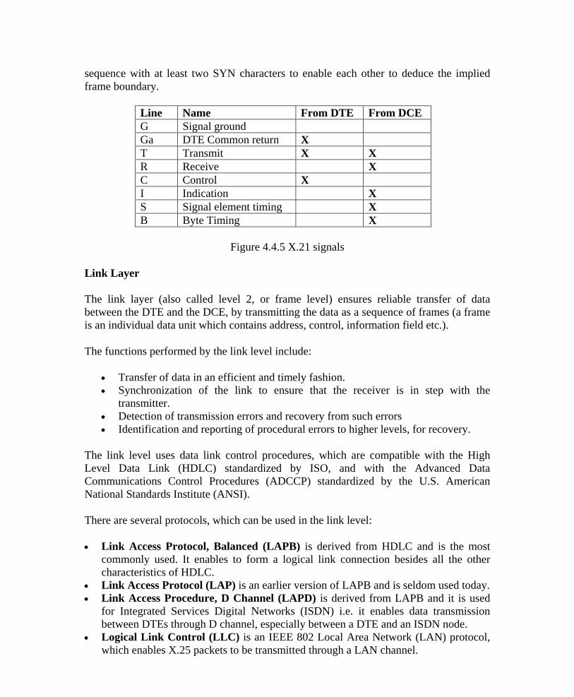
sequence with at least two SYN characters to enable each other to deduce the implied frame boundary.

Line Name From DTE From DCE G Signal ground Ga DTE Common return X T Transmit X X R Receive X C Control X I Indication X S Signal element timing X B Byte Timing X

Figure 4.4.5 X.21 signals

Link Layer

The link layer (also called level 2, or frame level) ensures reliable transfer of data between the DTE and the DCE, by transmitting the data as a sequence of frames (a frame is an individual data unit which contains address, control, information field etc.).

The functions performed by the link level include:

• Transfer of data in an efficient and timely fashion. • Synchronization of the link to ensure that the receiver is in step with the

transmitter. • Detection of transmission errors and recovery from such errors • Identification and reporting of procedural errors to higher levels, for recovery.

The link level uses data link control procedures, which are compatible with the High Level Data Link (HDLC) standardized by ISO, and with the Advanced Data Communications Control Procedures (ADCCP) standardized by the U.S. American National Standards Institute (ANSI).

There are several protocols, which can be used in the link level:

• Link Access Protocol, Balanced (LAPB) is derived from HDLC and is the most commonly used. It enables to form a logical link connection besides all the other characteristics of HDLC.

• Link Access Protocol (LAP) is an earlier version of LAPB and is seldom used today. • Link Access Procedure, D Channel (LAPD) is derived from LAPB and it is used

for Integrated Services Digital Networks (ISDN) i.e. it enables data transmission between DTEs through D channel, especially between a DTE and an ISDN node.

• Logical Link Control (LLC) is an IEEE 802 Local Area Network (LAN) protocol, which enables X.25 packets to be transmitted through a LAN channel.


Now let us discuss the most commonly used link layer protocol, i.e. LAPB. LAPB is a bit-oriented protocol that ensures that frames are correctly ordered and error-free. There are three kinds of frames:

1. Information: This kind of frame contains the actual information being transferred and some control information. The control field in these frames contains the frame sequence number. I-frame functions include sequencing, flow control, and error detection and recovery. I-frames carry send- and receive-sequence numbers.

2. Supervisory: The supervisory frame (S-frame) carries control information. S-frame functions include requesting and suspending transmissions, reporting on status, and acknowledging the receipt of I-frames. S-frames carry only receive-sequence numbers. There are various types of supervisory frames.

o RECEIVE READY-Acknowledgment frame indicating the next frame expected.

o REJECT-Negative acknowledgment frame used to indicate transmission error detection.

o RECEIVE NOT READY (RNR)-Just as RECEIVE READY but tells the sender to stop sending due to temporary problems.

3. Unnumbered: This kind of frames is used only for control purposes. U-frame functions include link setup and disconnection, as well as error reporting. U frames carry no sequence numbers.

Packet Level

This level governs the end-to-end communications between the different DTE devices. Layer 3 is concerned with connection set-up and teardown and flow control between the DTE devices, as well as network routing functions and the multiplexing of simultaneous logical connections over a single physical connection. PLP is the network layer protocol of X.25.

Call setup mode is used to establish SVCs between DTE devices. A PLP uses the X.121 addressing scheme to set up the virtual circuit. The call setup mode is executed on a per-virtual-circuit basis, which means that one virtual circuit can be in call setup mode while another is in data transfer mode. This mode is used only with SVCs, not with PVCs. To establish a connection on an SVC, the calling DTE sends a Call Request Packet, which includes the address of the remote DTE to be contacted. The destination DTE decides whether or not to accept the call (the Call Request packet includes the sender's DTE address, as well as other information that the called DTE can use to decide whether or not to accept the call). A call is accepted by issuing a Call Accepted packet, or cleared by issuing a Clear Request packet. Once the originating DTE receives the Call Accepted packet, the virtual circuit is established and data transfer may take place.


DCE DCE

DTE DTE

Figure 4.4.6 Different Modes of PLP

Different phases of call set-up, data transfer, call release has been shown in Fig. 4.4.6. The PLP operates in five distinct modes: call setup, data transfer, idle, call clearing, and restarting.

• Data transfer mode is used for transferring data between two DTE devices across a virtual circuit. In this mode, PLP handles segmentation and reassembly, bit padding, and error and flow control. This mode is executed on a per-virtual-circuit basis and is used with both PVCs and SVCs.

• Idle mode is used when a virtual circuit is established but data transfer is not occurring. It is executed on a per-virtual-circuit basis and is used only with SVCs.

• Call clearing mode is used to end communication sessions between DTE devices and to terminate SVCs. This mode is executed on a per-virtual-circuit basis and is used only with SVCs. When either DTE wishes to terminate the call, a Clear Request packet is sent to the remote DTE, which responds with a Clear Confirmation packet.

• Restarting mode is used to synchronize transmission between a DTE device and a locally connected DCE device. This mode is not executed on a per-virtual-circuit basis. It affects all the DTE device's established virtual circuits.

Four types of PLP packet fields exist:

• General Format Identifier (GFI)—Identifies packet parameters, such as whether the packet carries user data or control information, what kind of windowing is being used, and whether delivery confirmation is required.

• Logical Channel Identifier (LCI)—identifies the virtual circuit across the local DTE/DCE interface.

• Packet Type Identifier (PTI)—identifies the packet as one of 17 different PLP packet types.

Clear Indication

Clear Response Clear Confirm

Clear Request

Data Data

Data

Data

Call Connected

Call request

Incoming Call

Call accepted


• User Data—Contains encapsulated upper-layer information. This field is present only in data packets. Otherwise, additional fields containing control information are added.

Fill in the Blank: 1. X.25 is a standard for ________communications. 2. X.25 protocol uses _________ for end-to-end transmission. 3. X.25 operates in ___________ layer of OSI. 4. ____________________ devices are end systems that communicate across the

X.25 network. 5. Two types of X.25 virtual circuits exist: _________ and ______________. 6. At the physical layer _______ is specifically defined for X.25 by ITU-T. 7. The link level ensures reliable transfer of data between the _____ and the ____. 8. The ____________ frame carries control information. 9. ______________frame contains the actual information being transferred 10. The PLP Packet is a product of ________ layer in X.25 standard. 11. The PLP ___________ is used to transport data from the upper layers in X.25

standard.

Short Answers Questions:

1. In what layers X.25 operates? Ans: X.25 operates in the network layer. 2. What are the key functions of X.25 protocol? Ans: Key functions of X.25 protocol are:

i) Call control packets are used for call set-up. ii) Multiplexing of virtual circuits take place in packet layer. iii) Both link layer and packet layer performs flow control and error control.

3. What limitation of X.25 is overcome in Frame Relay Protocol? Ans: In X.25, overhead on the user equipment and the networking equipment is very high and it is also slower (can go up to 64 kbps only), which are overcome in Frame Control Protocol. 4. Explain the functionalities of DTE, DCE, PSE. Ans: Data terminal equipment devices are end systems that communicate across the X.25 network. They are usually terminals, personal computers, or network hosts, and are located on the premises of individual subscribers. DCE devices are communications devices, such as modems and packet switches that provide the interface between DTE devices and a PSE, and are generally located in the carrier's facilities. PSEs are switches that compose the bulk of the carrier's network. They transfer data from one DTE device to another through the X.25 PSN


5. Describe the functionalities of Link Level. Ans: The functions performed by the link level include:

• Transfer of data in an efficient and timely fashion. • Synchronization of the link to ensure that the receiver is in step with the

transmitter. • Detection of transmission errors and recovery from such errors • Identification and reporting of procedural errors to higher levels, for recovery.

6. What protocols can be used in Link Level?

Ans: There are several protocols which can be used in the link level:

• Link Access Protocol, Balanced (LAPB) is derived from HDLC and is the most commonly used. It enables to form a logical link connection besides all the other characteristics of HDLC.

• Link Access Protocol (LAP) is an earlier version of LAPB and is seldom used today. • Link Access Procedure, D Channel (LAPD) is derived from LAPB and it is used

for Integrated Services Digital Networks (ISDN) i.e. it enables data transmission between DTEs through D channel, especially between a DTE and an ISDN node.

• Logical Link Control (LLC) is an IEEE 802 Local Area Network (LAN) protocol which enables X.25 packets to be transmitted through a LAN channel.

7. Explain the different level of operation of PLP.

Ans: The PLP operates in five distinct modes: call setup, data transfer, idle, call clearing, and restarting.

• Call setup mode is used to establish SVCs between DTE devices. A PLP uses the X.121 addressing scheme to set up the virtual circuit. The call setup mode is executed on a per-virtual-circuit basis.

• Data transfer mode is used for transferring data between two DTE devices across a virtual circuit. In this mode, PLP handles segmentation and reassembly, bit padding, and error and flow control.

• Idle mode is used when a virtual circuit is established but data transfer is not occurring

• Call clearing mode is used to end communication sessions between DTE devices and to terminate SVCs. This mode is executed on a per-virtual-circuit basis and is used only with SVCs.

• Restarting mode is used to synchronize transmission between a DTE device and a locally connected DCE device. This mode is not executed on a per-virtual-circuit basis. It affects all the DTE device's established virtual circuits.


Special Instructional Objective • On completion of this lesson, the student will be able to: • State the limitations of X.25 • Explain the key features of Frame Relay • Specify the Frame relay frame format • Explain how congestion control is performed in Frame relay network

4.5.1 Introduction Frame Relay is a high-performance WAN protocol that operates at the physical and data link layers of the OSI reference model. Frame Relay originally was designed for use across Integrated Services Digital Network (ISDN) interfaces. Today, it is used over a variety of other network interfaces as well. Frame Relay is a simplified form of Packet Switching, similar in principle to X.25, in which synchronous frames of data are routed to different destinations depending on header information. The biggest difference between Frame Relay and X.25 is that X.25 guarantees data integrity and network managed flow control at the cost of some network delays. Frame Relay switches packets end to end much faster, but there is no guarantee of data integrity at all. As line speeds have increased from speeds below 64kbps to T1/E1 and beyond, the delays inherent in the store-and-forward mechanisms of X.25 become intolerable. At the same time, improvements in digital transmission techniques have reduced line errors to the extent that node-to-node error correction throughout the network is no longer necessary. The vast majority of Frame Relay traffic consists of TCP/IP or other protocols that provide their own flow control and error correction mechanisms. Much of this traffic is fed into the Internet, another packet switched network without any built-in error control. Because Frame Relay does not 'care' whether the frame it is switching is error-free or not, a Frame Relay node can start switching traffic out onto a new line as soon as it has read the first two bytes of addressing information at the beginning of the frame. Thus a frame of data can travel end-to-end, passing through several switches, and still arrive at its destination with only a few bytes' delay. These delays are small enough that network latency under Frame Relay is not noticeably different from direct leased line connections. As a result, the performance of a Frame Relay network is virtually identical to that of a leased line, but because most of the network is shared, costs are lower. Frame Relay is an example of a packet-switched technology. Packet-switched networks enable end stations to dynamically share the network medium and the available bandwidth. The following two techniques are used in packet-switching technology:

• Variable-length packets • Statistical multiplexing

Variable-length packets are used for more efficient and flexible data transfers. These packets are switched between the various segments in the network until the destination is reached.


Statistical multiplexing techniques control network access in a packet-switched network. The advantage of this technique is that it accommodates more flexibility and more efficient use of bandwidth. Most of today's popular LANs, such as Ethernet and Token Ring, are packet-switched networks. 4.5.2 Frame Relay Devices

Devices attached to a Frame Relay WAN fall into the following two general categories:

• Data terminal equipment (DTE) • Data circuit-terminating equipment (DCE)

DTEs generally are considered to be terminating equipment for a specific network and typically are located on the premises of a customer. In fact, they may be owned by the customer. Examples of DTE devices are terminals, personal computers, routers, and bridges.

DCEs are carrier-owned internetworking devices. The purpose of DCE equipment is to provide clocking and switching services in a network, which are the devices that actually transmit data through the WAN. In most cases, these are packet switches.

The connection between a DTE device and a DCE device consists of both a physical layer component and a link layer component. The physical component defines the mechanical, electrical, functional, and procedural specifications for the connection between the devices. One of the most commonly used physical layer interface specifications is the recommended standard (RS)-232 specification. The link layer component defines the protocol that establishes the connection between the DTE device, such as a router, and the DCE device, such as a switch.

4.5.3 Virtual Circuits

Frame Relay is a virtual circuit network, so it doesn’t use physical addresses to define the DTEs connected to the network. Frame Relay provides connection-oriented data link layer communication. This means that a defined communication exists between each pair of devices and that these connections are associated with a connection identifier. However, virtual circuit identifiers in Frame relay operate at the data link layer, in contrast with X.25, where they operate at the network layer. This service is implemented by using a Frame Relay virtual circuit, which is a logical connection created between two data terminal equipment (DTE) devices across a Frame Relay packet-switched network (PSN).

Virtual circuits provide a bidirectional communication path from one DTE device to another and are uniquely identified by a data-link connection identifier (DLCI). A


number of virtual circuits can be multiplexed into a single physical circuit for transmission across the network. This capability often can reduce the equipment and network complexity required to connect multiple DTE devices.

A virtual circuit can pass through any number of intermediate DCE devices (switches) located within the Frame Relay PSN. Before going into the details of DLCI let us first have a look at the two types of Frame Relay Circuits, namely: switched virtual circuits (SVCs) and permanent virtual circuits (PVCs).

4.5.3.1 Switched Virtual Circuits

Switched virtual circuits (SVCs) are temporary connections used in situations requiring only sporadic data transfer between DTE devices across the Frame Relay network. A communication session across an SVC consists of the following four operational states:

• Call setup—The virtual circuit between two Frame Relay DTE devices is established.

• Data transfer—Data is transmitted between the DTE devices over the virtual circuit. • Idle—The connection between DTE devices is still active, but no data is transferred.

If an SVC remains in an idle state for a defined period of time, the call can be terminated.

• Call termination—The virtual circuit between DTE devices is terminated.

After the virtual circuit is terminated, the DTE devices must establish a new SVC if there is additional data to be exchanged. It is expected that SVCs will be established, maintained, and terminated using the same signaling protocols used in ISDN.

4.5.3.2 Permanent Virtual Circuits

Permanent virtual circuits (PVCs) are permanently established connections that are used for frequent and consistent data transfers between DTE devices across the Frame Relay network. Communication across PVC does not require the call setup and termination states that are used with SVCs. PVCs always operate in one of the following two operational states:

Data transfer: Data is transmitted between the DTE devices over the virtual circuit. Idle: The connection between DTE devices is active, but no data is transferred.

Unlike SVCs, PVCs will not be terminated under any circumstances when in an idle state. DTE devices can begin transferring data whenever they are ready because the circuit is permanently established.

4.5.3.3 Data-Link Connection Identifier (DLCI)

Frame Relay virtual circuits are identified by data-link connection identifiers (DLCIs). DLCI values typically are assigned by the Frame Relay service provider (for example, the


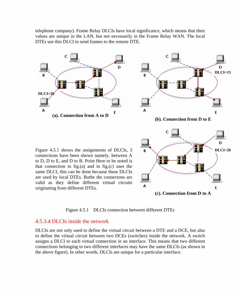
telephone company). Frame Relay DLCIs have local significance, which means that their values are unique in the LAN, but not necessarily in the Frame Relay WAN. The local DTEs use this DLCI to send frames to the remote DTE.

Figure 4.5.1 shows the assignments of DLCIs, 3 connections have been shown namely, between A to D, D to E, and D to B. Point Here to be noted is that connection in fig.(a) and in fig.(c) uses the same DLCI, this can be done because these DLCIs are used by local DTEs. Bothe the connectons are valid as they define different virtual circuits originating from different DTEs.

DLCI=15

Figure 4.5.1 DLCIs connection between different DTEs

4.5.3.4 DLCIs inside the network DLCIs are not only used to define the virtual circuit between a DTE and a DCE, but also to define the virtual circuit between two DCEs (switches) inside the network. A switch assigns a DLCI to each virtual connection in an interface. This means that two different connections belonging to two different interfaces may have the same DLCIs (as shown in the above figure). In other words, DLCIs are unique for a particular interface.

DLCI=26

(a). Connection from A to D (b). Connection from D to E

DLCI=26

(c). Connection from D to A


A connection between DTE A and DTE D has been shown in this figure, DLCI assigned inside the Frame Relay network is also shown in the network. DCEs inside the network use incoming interface – DLCI combination to decide the outgoing interface – DLCI combination to switch out the frame, from that DCE.

DLCI =122

Figure 4.5.2 DLCIs inside Frame relay network

Each switch in a Frame relay network has a table to route frames The table matches the incoming interface- DLCI combination with an outgoing interface-DLCI combination. Figure 4.5.3 shows two frames arriving at the switch on interface2, one with DLCI=11 and other with DLCI= 213.

Incoming Outgoing Interface DLCI Interface DLCI 1 122 1 41 2 213 1 158 2 11 2 111 1 151 2 210

Figure 4.5.3 Frame Relay switch table

4.5.4 Frame Relay Layers Frame Relay has only 2 layers, namely Physical layer and Data Link layer. And as compared to other layer of packet switching network such as X.25, frame relay has only 1.5 layers whereas X.25 has 2 layers. Frame Relay eliminates all network layer functions and a portion of conventional data-link layer functions.

9 77

DLCI=26

1

22

1DLCI=213

DLCI= 213 DLCI= 11 DLCI=111


Physical Layer No specific protocol is defined for physical layer in frame relay. Frame relay supports any one of the protocols recognized by ANSI, and thus the choice of physical layer protocol is up to the implementer. Data Link Layer At Data-link Layer Frame employs a simpler version of HDLC. Simpler version is used because HDLC provides extensive error and flow control fields that are not needed in frame relay.

To understand much of the functionality of Frame Relay, it is helpful to understand the structure of the Frame Relay frame. Figure 4.5.4 depicts the basic format of the Frame Relay frame. Flags indicate the beginning and end of the frame. Three primary components make up the Frame Relay frame: the header and address area, the user-data portion, and the frame check sequence (FCS). The address area, which is 2 bytes in length, is comprised of 10 bits representing the actual circuit identifier and 6 bits of fields related to congestion management. This identifier commonly is referred to as the data-link connection identifier (DLCI).

Figure 4.5.4 Frame Relay frame format

• Flags—Delimits the beginning and end of the frame. The value of this field is always the same and is represented either as the hexadecimal number 7E or as the binary number 01111110.

• Address—Contains the following information:

DLCI—The 10-bit DLCI is the essence of the Frame Relay header. This value represents the virtual connection between the DTE device and the switch. Each virtual connection


that is multiplexed onto the physical channel will be represented by a unique DLCI. The DLCI values have local significance only, which means that they are unique only to the physical channel on which they reside. Therefore, devices at opposite ends of a connection can use different DLCI values to refer to the same virtual connection. The first 6-bits of the first byte make up part 1 of the DLCI, and second part of DLCI uses the first 4-bits of second byte.

Extended Address (EA)—The EA is used to indicate whether the byte in which the EA value is 1 is the last addressing field. If the value is 1, then the current byte is determined to be the last DLCI octet. Although current Frame Relay implementations all use a two-octet DLCI, this capability does allow longer DLCIs to be used in the future. The eighth bit of each byte of the Address field is used to indicate the EA.

C/R—The C/R is the bit that follows the most significant DLCI byte in the Address field. The C/R bit is not currently defined.

Congestion Control—This consists of the 3 bits that control the Frame Relay congestion-notification mechanisms. These are the FECN, BECN, and DE bits, which are the last 3 bits in the Address field.

Forward-explicit congestion notification (FECN) is a single-bit field that can be set to a value of 1 by a switch to indicate to an end DTE device, such as a router, that congestion was experienced in the direction of the frame transmission from source to destination as shown in Fig. 4.5.5. The primary benefit of the use of the FECN and BECN fields is the capability of higher-layer protocols to react intelligently to these congestion indicators. Today, DECnet and OSI are the only higher-layer protocols that implement these capabilities.

Figure 4.5.5 Forward-explicit congestion notification

Backward-explicit congestion notification (BECN) is a single-bit field that, when set to a value of 1 by a switch, indicates that congestion was experienced in the network in the direction opposite of the frame transmission from source to destination.

Discard eligibility (DE) is set by the DTE device, such as a router, to indicate that the marked frame is of lesser importance relative to other frames being transmitted. Frames


that are marked as "discard eligible" should be discarded before other frames in a congested network. This allows for a basic prioritization mechanism in Frame Relay networks.

Figure 4.5.6 Backward-explicit congestion notification

•Data—Contains encapsulated upper-layer data. Each frame in this variable-length field includes a user data or payload field that will vary in length up to 16,000 octets. This field serves to transport the higher-layer protocol packet (PDU) through a Frame Relay network.

• Frame Check Sequence—Ensures the integrity of transmitted data. This value is computed by the source device and verified by the receiver to ensure integrity of transmission.

4.5.5 Summary

• Frame relay operates only in data link and physical layer. • Frame Relay allows bursty traffic. • It allows frame size of 9000 bytes, which can accommodate all local area network

frames. • Frame relay is less expensive then other traditional WANs. • Frame relay provides both Permanent and switched connections. • Frame relay allow variable-length frames, this may create varying delays for

different users. Due to variable delay it is not suitable for real-time communication


Fill in the blanks: 1. Frame Relay is a high-performance ______ protocol. 2. Frame Relay operates at the __________ and _____________ layers of the OSI

reference model. 3. Frame Relay requires Error Checking at the _________ layer. 4. Frame Relay is a simplified form of ______________ switching, similar in

principle to _______. 5. Frame Relay is a ___________________ network. 6. Frame Relay virtual circuits are identified by ___________. 7. ______ bit in address field in frame relay is set to one to signify the last address

bit. 8. Routing and switching in Frame Relay is performed by ________ layer. 9. ________ data are allowed on a Frame Relay Network. 10. Frame relay is not suited well for ______ due to the delay resulting from varying

sizes of Frame. Answers fill in the blanks 1. WAN 2. Physical, data link 3. Data link 4. Circuit, X.25 5. Virtual switched 6. DLCIs. 7. Extended Address (EA) 8. Data link layer 9. Encapsulated upper layer 10. Real time traffic

Short Answer Questions: 1. Explain few devices used in Frame relay. Ans: Devices attached to a Frame Relay WAN fall into the following two general categories: • Data terminal equipment (DTE) : DTEs generally are considered to be terminating

equipment for a specific network and typically are located on the premises of a customer

• Data circuit-terminating equipment (DCE): DCEs are carrier-owned internetworking devices. The purpose of DCE equipment is to provide clocking and switching services in a network, which are the devices that actually transmit data through the WAN. In most cases, these are packet switches.


2. Distinguish between permanent virtual and switched virtual connections used in Frame relay protocol. Ans: In permanent virtual connection, the path is fixed and data transfer occurs as with virtual calls, but no call setup or termination is required. On the other hand, in switched virtual connection, the path is a dynamically established virtual circuit using a call set up and call clearing procedure. Many other circuits can share the same path. 3. What are the various states in a Switched virtual circuit connection in Frame Relay? Ans: A communication session across an SVC consists of the following four operational states:

• Call setup—The virtual circuit between two Frame Relay DTE devices is established.

• Data transfer—Data is transmitted between the DTE devices over the virtual circuit. • Idle—The connection between DTE devices is still active, but no data is transferred.

If an SVC remains in an idle state for a defined period of time, the call can be terminated.

• Call termination—The virtual circuit between DTE devices is terminated.

4. Describe Permanent Virtual switched connection in Frame Relay. Ans: Permanent virtual circuits (PVCs) are permanently established connections that are used for frequent and consistent data transfers between DTE devices across the Frame Relay network. Communication across PVC does not require the call setup and termination states that are used with SVCs. PVCs always operate in one of the following two operational states:

• Data transfer—Data is transmitted between the DTE devices over the virtual circuit.

• Idle—The connection between DTE devices is active, but no data is transferred.

Unlike SVCs, PVCs will not be terminated under any circumstances when in an idle state. DTE devices can begin transferring data whenever they are ready because the circuit is permanently established.

5. Write a short Note on Data-Link Connection Identifier (DLCI).

Ans: Frame Relay virtual circuits are identified by data-link connection identifiers (DLCIs). DLCI values typically are assigned by the Frame Relay service provider (for example, the telephone company). Frame Relay DLCIs have local significance, which means that their values are unique in the LAN, but not necessarily in the Frame Relay WAN. The local DTEs use this DLCI to send frames to the remote DTE.


DLCIs are not only used to define the virtual circuit between a DTE and a DCE, but also to define the virtual circuit between two DCEs (switches) inside the network. A switch assigns a DLCI to each virtual connection in an interface. This means that two different connections belonging to two different interfaces may have the same DLCIs. In other words, DLCIs are unique for a particular interface.

6. What does extended address field in Frame Relay frame Format specifies?

Ans: Extended Address (EA) is used to indicate whether the byte in which the EA value is 1 is the last addressing field. If the value is 1, then the current byte is determined to be the last DLCI octet. Although current Frame Relay implementations all use a two-octet DLCI, this capability does allow longer DLCIs to be used in the future. The eighth bit of each byte of the Address field is used to indicate the EA.


UNIT-2

Special Instructional Objectives:

On completion, the student will be able to: • State the need for flow and error control • Explain how Stop-and-wait flow control works • Explain how Sliding-window protocol is used for flow control • Explain how Stop-and-wait ARQ works • Explain how Go-back-N ARQ works • Explain how Selective-repeat ARQ works

3.3.1 Introduction

As we have mentioned earlier, for reliable and efficient data communication a great deal of coordination is necessary between at least two machines. Some of these are necessary because of the following constraints:

• Both sender and receiver have limited speed • Both sender and receiver have limited memory

It is necessary to satisfy the following requirements: • A fast sender should not overwhelm a slow receiver, which must perform a

certain amount of processing before passing the data on to the higher-level software.

• If error occur during transmission, it is necessary to devise mechanism to correct it

The most important functions of Data Link layer to satisfy the above requirements are error control and flow control. Collectively, these functions are known as data link control, as discussed in this lesson.

Flow Control is a technique so that transmitter and receiver with different speed characteristics can communicate with each other. Flow control ensures that a transmitting station, such as a server with higher processing capability, does not overwhelm a receiving station, such as a desktop system, with lesser processing capability. This is where there is an orderly flow of transmitted data between the source and the destination.

Error Control involves both error detection and error correction. It is necessary because errors are inevitable in data communication, in spite of the use of better equipment and reliable transmission media based on the current technology. In the preceding lesson we have already discussed how errors can be detected. In this lesson we shall discuss how error control is performed based on retransmission of the corrupted data. When an error is detected, the receiver can have the specified frame retransmitted by the sender. This process is commonly known as Automatic Repeat Request (ARQ). For example, Internet's Unreliable Delivery Model allows packets to be discarded if network resources are not available, and demands that ARQ protocols make provisions for retransmission.


3.3.2 Flow Control

Modern data networks are designed to support a diverse range of hosts and communication mediums. Consider a 933 MHz Pentium-based host transmitting data to a 90 MHz 80486/SX. Obviously, the Pentium will be able to drown the slower processor with data. Likewise, consider two hosts, each using an Ethernet LAN, but with the two Ethernets connected by a 56 Kbps modem link. If one host begins transmitting to the other at Ethernet speeds, the modem link will quickly become overwhelmed. In both cases, flow control is needed to pace the data transfer at an acceptable speed.

Flow Control is a set of procedures that tells the sender how much data it can transmit before it must wait for an acknowledgment from the receiver. The flow of data should not be allowed to overwhelm the receiver. Receiver should also be able to inform the transmitter before its limits (this limit may be amount of memory used to store the incoming data or the processing power at the receiver end) are reached and the sender must send fewer frames. Hence, Flow control refers to the set of procedures used to restrict the amount of data the transmitter can send before waiting for acknowledgment.

There are two methods developed for flow control namely Stop-and-wait and Sliding-window. Stop-and-wait is also known as Request/reply sometimes. Request/reply (Stop-and-wait) flow control requires each data packet to be acknowledged by the remote host before the next packet is sent. This is discussed in detail in the following subsection. Sliding window algorithms, used by TCP, permit multiple data packets to be in simultaneous transit, making more efficient use of network bandwidth as discussed in subsection 3.3.2.2.

3.3.2.1 Stop-and-Wait

This is the simplest form of flow control where a sender transmits a data frame. After receiving the frame, the receiver indicates its willingness to accept another frame by sending back an ACK frame acknowledging the frame just received. The sender must wait until it receives the ACK frame before sending the next data frame.This is sometimes referred to as ping-pong behavior, request/reply is simple to understand and easy to implement, but not very efficient. In LAN environment with fast links, this isn't much of a concern, but WAN links will spend most of their time idle, especially if several hops are required.

Figure 3.3.1 illustrates the operation of the stop-and-wait protocol. The blue arrows show the sequence of data frames being sent across the link from the sender (top to the receiver (bottom). The protocol relies on two-way transmission (full duplex or half duplex) to allow the receiver at the remote node to return frames acknowledging the successful transmission. The acknowledgements are shown in green in the diagram, and flow back to the original sender. A small processing delay may be introduced between reception of the last byte of a Data PDU and generation of the corresponding ACK.


Major drawback of Stop-and-Wait Flow Control is that only one frame can be in transmission at a time, this leads to inefficiency if propagation delay is much longer than the transmission delay.

Figure 3. 3.1 Stop-and Wait protocol

Some protocols pretty much require stop-and-wait behavior. For example, Internet's Remote Procedure Call (RPC) Protocol is used to implement subroutine calls from a program on one machine to library routines on another machine. Since most programs are single threaded, the sender has little choice but to wait for a reply before continuing the program and possibly sending another request.

Link Utilization in Stop-and-Wait Let us assume the following: Transmission time: The time it takes for a station to transmit a frame (normalized to a value of 1). Propagation delay: The time it takes for a bit to travel from sender to receiver (expressed as a).

– a < 1 :The frame is sufficiently long such that the first bits of the frame arrive at the destination before the source has completed transmission of the frame.

– a > 1: Sender completes transmission of the entire frame before the leading bits of the frame arrive at the receiver.

– The link utilization U = 1/(1+2a), a = Propagation time / transmission time

It is evident from the above equation that the link utilization is strongly dependent on the ratio of the propagation time to the transmission time. When the propagation time is small, as in case of LAN environment, the link utilization is good. But, in case of long propagation delays, as in case of satellite communication, the utilization can be very poor. To improve the link utilization, we can use the following (sliding-window) protocol instead of using stop-and-wait protocol.

3.3.2.2 Sliding Window

With the use of multiple frames for a single message, the stop-and-wait protocol does not perform well. Only one frame at a time can be in transit. In stop-and-wait flow control, if a > 1, serious inefficiencies result. Efficiency can be greatly improved by allowing multiple frames to be in transit at the same time. Efficiency can also be improved by making use of the full-duplex line. To keep track of the frames, sender station sends sequentially numbered frames. Since the sequence number to be used occupies a field in the frame, it should be of limited size. If the header of the frame allows k bits, the


sequence numbers range from 0 to 2k – 1. Sender maintains a list of sequence numbers that it is allowed to send (sender window). The size of the sender’s window is at most 2k

– 1. The sender is provided with a buffer equal to the window size. Receiver also maintains a window of size 2k – 1. The receiver acknowledges a frame by sending an ACK frame that includes the sequence number of the next frame expected. This also explicitly announces that it is prepared to receive the next N frames, beginning with the number specified. This scheme can be used to acknowledge multiple frames. It could receive frames 2, 3, 4 but withhold ACK until frame 4 has arrived. By returning an ACK with sequence number 5, it acknowledges frames 2, 3, 4 in one go. The receiver needs a buffer of size 1.

Sliding window algorithm is a method of flow control for network data transfers. TCP, the Internet's stream transfer protocol, uses a sliding window algorithm.

A sliding window algorithm places a buffer between the application program and the network data flow. For TCP, the buffer is typically in the operating system kernel, but this is more of an implementation detail than a hard-and-fast requirement.

Figure 3.3.2 Buffer in sliding window

Data received from the network is stored in the buffer, from where the application can read at its own pace. As the application reads data, buffer space is freed up to accept more input from the network. The window is the amount of data that can be "read ahead" - the size of the buffer, less the amount of valid data stored in it. Window announcements are used to inform the remote host of the current window size.

Sender sliding Window: At any instant, the sender is permitted to send frames with sequence numbers in a certain range (the sending window) as shown in Fig. 3.3.3.

Figure 3.3.3 Sender’s window


Receiver sliding Window: The receiver always maintains a window of size 1 as shown in Fig. 3.3.4. It looks for a specific frame (frame 4 as shown in the figure) to arrive in a specific order. If it receives any other frame (out of order), it is discarded and it needs to be resent. However, the receiver window also slides by one as the specific frame is received and accepted as shown in the figure. The receiver acknowledges a frame by sending an ACK frame that includes the sequence number of the next frame expected. This also explicitly announces that it is prepared to receive the next N frames, beginning with the number specified. This scheme can be used to acknowledge multiple frames. It could receive frames 2, 3, 4 but withhold ACK until frame 4 has arrived. By returning an ACK with sequence number 5, it acknowledges frames 2, 3, 4 at one time. The receiver needs a buffer of size 1.

Figure 3.3.4 Receiver sliding window

On the other hand, if the local application can process data at the rate it's being transferred; sliding window still gives us an advantage. If the window size is larger than the packet size, then multiple packets can be outstanding in the network, since the sender knows that buffer space is available on the receiver to hold all of them. Ideally, a steady-state condition can be reached where a series of packets (in the forward direction) and window announcements (in the reverse direction) are constantly in transit. As each new window announcement is received by the sender, more data packets are transmitted. As the application reads data from the buffer (remember, we're assuming the application can keep up with the network), more window announcements are generated. Keeping a series of data packets in transit ensures the efficient use of network resources.

Hence, Sliding Window Flow Control o Allows transmission of multiple frames o Assigns each frame a k-bit sequence number o Range of sequence number is [0…2k-1], i.e., frames are counted modulo 2k.

The link utilization in case of Sliding Window Protocol U = 1, for N > 2a + 1 N/(1+2a), for N < 2a + 1 Where N = the window size, and a = Propagation time / transmission time


3.3.3 Error Control Techniques

When an error is detected in a message, the receiver sends a request to the transmitter to retransmit the ill-fated message or packet. The most popular retransmission scheme is known as Automatic-Repeat-Request (ARQ). Such schemes, where receiver asks transmitter to re-transmit if it detects an error, are known as reverse error correction techniques. There exist three popular ARQ techniques, as shown in Fig. 3.3.5.

Figure 3.3.5 Error control techniques

3.3.3.1 Stop-and-Wait ARQ

F1A0

Time

In Stop-and-Wait ARQ, which is simplest among all protocols, the sender (say station A) transmits a frame and then waits till it receives positive acknowledgement (ACK) or negative acknowledgement (NACK) from the receiver (say station B). Station B sends an ACK if the frame is received correctly, otherwise it sends NACK. Station A sends a new frame after receiving ACK; otherwise it retransmits the old frame, if it receives a NACK. This is illustrated in Fig 3.3.6.

Frame F0 Station A

Station B

Processing delay tproc

Propagation delay tprop

F0 F2 Frame A0 A1

Figure 3.3.6 Stop-And-Wait ARQ technique

To tackle the problem of a lost or damaged frame, the sender is equipped with a timer. In case of a lost ACK, the sender transmits the old frame. In the Fig. 3.3.7, the second PDU of Data is lost during transmission. The sender is unaware of this loss, but starts a timer after sending each PDU. Normally an ACK PDU is received before the


timer expires. In this case no ACK is received, and the timer counts down to zero and triggers retransmission of the same PDU by the sender. The sender always starts a timer following transmission, but in the second transmission receives an ACK PDU before the timer expires, finally indicating that the data has now been received by the remote node.

Figure 3.3.7 Retransmission due to lost frame

The receiver now can identify that it has received a duplicate frame from the label of the frame and it is discarded

To tackle the problem of damaged frames, say a frame that has been corrupted during the transmission due to noise, there is a concept of NACK frames, i.e. Negative Acknowledge frames. Receiver transmits a NACK frame to the sender if it founds the received frame to be corrupted. When a NACK is received by a transmitter before the time-out, the old frame is sent again as shown in Fig. 3.3.8.

Figure 3.3.8 Retransmission due to damaged frame

No error detected

F0NA0Frame F0 Time

Station A

Retransmission due to receive of NACK frame

Station B

Processing delay tproc

Propagation delay tprop

F0 F0 A0 Frame NA0

ACK send for frame0

Error found in Frame 0


The main advantage of stop-and-wait ARQ is its simplicity. It also requires minimum buffer size. However, it makes highly inefficient use of communication links, particularly when ‘a’ is large.

3.3.3.2 Go-back-N ARQ

The most popular ARQ protocol is the go-back-N ARQ, where the sender sends the frames continuously without waiting for acknowledgement. That is why it is also called as continuous ARQ. As the receiver receives the frames, it keeps on sending ACKs or a NACK, in case a frame is incorrectly received. When the sender receives a NACK, it retransmits the frame in error plus all the succeeding frames as shown in Fig.3.3.9. Hence, the name of the protocol is go-back-N ARQ. If a frame is lost, the receiver sends NAK after receiving the next frame as shown in Fig. 3.3.10. In case there is long delay before sending the NAK, the sender will resend the lost frame after its timer times out. If the ACK frame sent by the receiver is lost, the sender resends the frames after its timer times out as shown in Fig. 3.3.11.

Assuming full-duplex transmission, the receiving end sends piggybacked acknowledgement by using some number in the ACK field of its data frame. Let us assume that a 3-bit sequence number is used and suppose that a station sends frame 0 and gets back an RR1, and then sends frames 1, 2, 3, 4, 5, 6, 7, 0 and gets another RR1.This might either mean that RR1 is a cumulative ACK or all 8 frames were damaged. This ambiguity can be overcome if the maximum window size is limited to 7, i.e. for a k-bit sequence number field it is limited to 2k-1. The number N (=2k-1) specifies how many frames can be sent without receiving acknowledgement.

Figure 3.3.9 Frames in error in go-Back-N ARQ


Figure 3.3.10 Lost Frames in Go-Back-N ARQ

Figure 3.3.11 Lost ACK in Go-Back-N ARQ

If no acknowledgement is received after sending N frames, the sender takes the help of a timer. After the time-out, it resumes retransmission. The go-back-N protocol


also takes care of damaged frames and damaged ACKs. This scheme is little more complex than the previous one but gives much higher throughput.

Assuming full-duplex transmission, the receiving end sends piggybacked acknowledgement by using some number in the ACK field of its data frame. Let us assume that a 3-bit sequence number is used and suppose that a station sends frame 0 and gets back an RR1, and then sends frames 1, 2, 3, 4, 5, 6, 7, 0 and gets another RR1.This might either mean that RR1 is a cumulative ACK or all 8 frames were damaged. This ambiguity can be overcome if the maximum window size is limited to 7, i.e. for a k-bit sequence number field it is limited to 2k-1. The number N (=2k-1) specifies how many frames can be sent without receiving acknowledgement. If no acknowledgement is received after sending N frames, the sender takes the help of a timer. After the time-out, it resumes retransmission. The go-back-N protocol also takes care of damaged frames and damaged ACKs. This scheme is little more complex than the previous one but gives much higher throughput.

3.3.3.3 Selective-Repeat ARQ

The selective-repetitive ARQ scheme retransmits only those for which NAKs are received or for which timer has expired, this is shown in the Fig.3.3.12. This is the most efficient among the ARQ schemes, but the sender must be more complex so that it can send out-of-order frames. The receiver also must have storage space to store the post-NAK frames and processing power to reinsert frames in proper sequence.

Figure 3.3.12 Selective-repeat Reject

F3F7 F6 F9 F5 F8 F4 F3 F2F1

Time

Station A

Station B ACK A3

NAK NA3

ACKA2

ACKA1

Retransmission of damaged frame only


Fill In The Blanks

1. _________Control is a technique for speed-matching of transmitter and receiver. 2. ________ Control provides for the addition of binary digits (redundant bits) that

can be used to identify if there has been an error in the transmission of one or more bits.

3. There are two methods developed for flow control namely _____________ and ____________.

4. Stop-And-Wait is also known as ____________. 5. Sliding Window Flow Control allows transmission of ____________ frames. 6. Sliding Window Flow Control assigns each frame a _____-bit sequence number. 7. Sliding window ARQ can be of two types namely, ____________ and

____________. Short Answer Questions 1. What are the key functions of error control techniques? Ans: There are basically two types of errors, namely, (a) Damaged Frame (b) Lost Frame. The key functions for error control techniques are as follows:

• Error detection • Sending of positive acknowledgement (ACK) by the receiver for no error • Sending of negative acknowledgement (NAK) by the receiver for error • Setting of timer for lost frame • Numbering of frames

2. Why is flow control needed? Ans: In case of data communication between a sender and a receiver, it may so happen that the rate at which data is transmitted by a fast sender is not acceptable by a slow receiver. IN such a situation, there is a need of flow control so that a fast transmitter does not overwhelm a slow receiver.

3. Mention key advantages and disadvantages of stop-and-wait ARQ

technique? Ans: Advantages of stop-and-wait ARQ are:

a. Simple to implement b. Frame numbering is modulo-2, i.e. only 1 bit is required.

The main disadvantage of stop-and-wait ARQ is that when the propagation delay is long, it is extremely inefficient.

4. Consider the use of 10 K-bit size frames on a 10 Mbps satellite channel with

270 ms delay. What is the link utilization for stop-and-wait ARQ technique assuming P = 10-3?


Ans: Link utilization = (1-P) / (1+2a) Where a = (Propagation Time) / (Transmission Time)

Propagation time = 270 msec Transmission time = (frame length) / (data rate) = (10 K-bit) / (10 Mbps) = 1 msec Hence, a = 270/1 = 270 Link utilization = 0.999/(1+2*270) ≈0.0018 =0.18%

5. What is the channel utilization for the go-back-N protocol with window size of 7 for the problem 3?

Ans: Channel utilization for go-back-N = N(1 – P) / (1 + 2a)(1-P+NP) P = probability of single frame error ≈ 10-3 Channel utilization ≈ 0.01285 = 1.285% 6. In what way selective-repeat is better than go-back-N ARQ technique? Ans : In selective-repeat scheme only the frame in error is retransmitted rather than transmitting all the subsequent frames. Hence it is more efficient than go-back-N ARQ technique.

7. In what situation Stop-and-Wait protocol works efficiently? Ans: In case of Stop-and-Wait protocol, the transmitter after sending a frame waits for the acknowledgement from the receiver before sending the next frame. This protocol works efficiently for long frames, where propagation time is small compared to the transmission time of the frame. 8. How the inefficiency of Stop-and-Wait protocol is overcome in sliding

window protocol? Ans: The Stop-and-Wait protocol is inefficient when large numbers of small packets are send by the transmitter since the transmitter has to wait for the acknowledgement of each individual packet before sending the next one. This problem can be overcome by sliding window protocol. In sliding window protocol multiple frames (up to a fixed number of frames) are send before receiving an acknowledgement from the receiver. 9. What is piggybacking? What is its advantage? Ans: In practice, the link between receiver and transmitter is full duplex and usually both transmitter and receiver stations send data to each over. So, instead of sending separate acknowledgement packets, a portion (few bits) of the data frames can be used for acknowledgement. This phenomenon is known as piggybacking. The piggybacking helps in better channel utilization. Further, multi-frame acknowledgement can be done.


10. For a k-bit numbering scheme, what is the range of sequence numbers used in sliding window protocol?

Ans: For k-bit numbering scheme, the total number of frames, N, in the sliding window can be given as follows (using modulo-k). N = 2k – 1 Hence the range of sequence numbers is: 0, 1, 2, and 3 … 2k – 1


Specific Instructional Objectives At the end of this lesson, the student will be able to:

• Explain the goals and requirements of Medium Access Control (MAC) techniques • Identify the key issues related to MAC techniques. • Give an outline of possible MAC techniques. • Distinguish between Centralized and Distributed MAC techniques. • Classify various contention based techniques such as ALHOA, CSMA,

CSMA/CD and CSMA/CA • Compare performance of contention based techniques • Explain round robin based MAC techniques.

o Polling o Token passing

5.2.1 Introduction A network of computers based on multi-access medium requires a protocol for effective sharing of the media. As only one node can send or transmit signal at a time using the broadcast mode, the main problem here is how different nodes get control of the medium to send data, that is “who goes next?”. The protocols used for this purpose are known as Medium Access Control (MAC) techniques. The key issues involved here are - Where and How the control is exercised.

‘Where’ refers to whether the control is exercised in a centralised or distributed manner. In a centralised system a master node grants access of the medium to other nodes. A centralized scheme has a number of advantages as mentioned below:

o Greater control to provide features like priority, overrides, and guaranteed

bandwidth. o Simpler logic at each node. o Easy coordination. Although this approach is easier to implement, it is vulnerable to the failure of the

master node and reduces efficiency. On the other hand, in a distributed approach all the nodes collectively perform a medium access control function and dynamically decide which node to be granted access. This approach is more reliable than the former one.

‘How’ refers to in what manner the control is exercised. It is constrained by the

topology and trade off between cost-performance and complexity. Various approaches for medium access control are shown in Fig. 5.2.1. The MAC techniques can be broadly divided into four categories; Contention-based, Round-Robin, Reservation-based and. Channelization-based. Under these four broad categories there are specific techniques, as shown in Fig. 5.2.1. In this lesson we shall concentrate of the MACs of the first two categories, which have been used in the legacy LANs of the IEEE standard. The CSMA/CA, a collision-free protocol used in wireless LAN, will be presented in Lesson 5.5. Channalization-based MACs, which are used in cellular telephone networks, will be


covered in Lesson 5.6. And the reservation-based MACs, which are used in satellite networks, will be discussed in Lesson 5.7.

Figure 5.2.1 Possible MAC techniques

5.2.2 Goals of MACs Medium Access Control techniques are designed with the following goals in mind.

• Initialisation: The technique enables network stations, upon power-up, to enter the state required for operation.

• Fairness: The technique should treat each station fairly in terms of the time it is made to wait until it gains entry to the network, access time and the time it is allowed to spend for transmission.

• Priority: In managing access and communications time, the technique should be able to give priority to some stations over other stations to facilitate different type of services needed.

• Limitations to one station: The techniques should allow transmission by one station at a time.

• Receipt: The technique should ensure that message packets are actually received (no lost packets) and delivered only once (no duplicate packets), and are received in the proper order.

• Error Limitation: The method should be capable of encompassing an appropriate error detection scheme.

• Recovery: If two packets collide (are present on the network at the same time), or if notice of a collision appears, the method should be able to recover, i.e. be able to halt all the transmissions and select one station to retransmit.


• Reconfigurability: The technique should enable a network to accommodate the addition or deletion of a station with no more than a noise transient from which the network station can recover.

• Compatibility: The technique should accommodate equipment from all vendors who build to its specification.

• Reliability: The technique should enable a network to confine operating inspite of a failure of one or several stations.

5.2.3 Round Robin Techniques In Round Robin techniques, each and every node is given the chance to send or transmit by rotation. When a node gets its turn to send, it may either decline to send, if it has no data or may send if it has got data to send. After getting the opportunity to send, it must relinquish its turn after some maximum period of time. The right to send then passes to the next node based on a predetermined logical sequence. The right to send may be controlled in a centralised or distributed manner. Polling is an example of centralised control and token passing is an example of distributed control as discussed below. 5.2.3.1 Polling The mechanism of polling is similar to the roll-call performed in a classroom. Just like the teacher, a controller sends a message to each node in turn. The message contains the address of the node being selected for granting access. Although all nodes receive the message, only the addressed node responds and then it sends data, if any. If there is no data, usually a “poll reject” message is sent back. In this way, each node is interrogated in a round-robin fashion, one after the other, for granting access to the medium. The first node is again polled when the controller finishes with the remaining codes.

The polling scheme has the flexibility of either giving equal access to all the nodes, or some nodes may be given higher priority than others. In other words, priority of access can be easily implemented.

Figure 5.2.2 Polling using a central controller


Polling can be done using a central controller, which may use a frequency band to send outbound messages as shown in Fig. 5.2.2. Other stations share a different frequency to send inbound messages. The technique is called frequency-division duplex approach (FDD). Main drawbacks of the polling scheme are high overhead of the polling messages and high dependence on the reliability of the controller.

Polling can also be accomplished without a central controller. Here, all stations receive signals from other stations as shown in Fig. 5.2.3. Stations develop a polling order list, using some protocol.

Figure 5.2.2 Polling in a distributed manner 5.2.3.2 Token Passing In token passing scheme, all stations are logically connected in the form of a ring and control of the access to the medium is performed using a token. A token is a special bit pattern or a small packet, usually several bits in length, which circulate from node to node. Token passing can be used with both broadcast (token bus) and sequentially connected (token ring) type of networks with some variation in the details as considered in the next lesson.

In case of token ring, token is passed from a node to the physically adjacent node. On the other hand, in the token bus, token is passed with the help of the address of the nodes, which form a logical ring. In either case a node currently holding the token has the ‘right to transmit’. When it has got data to send, it removes the token and transmits the data and then forwards the token to the next logical or physical node in the ring. If a node currently holding the token has no data to send, it simply forwards the token to the next node. The token passing scheme is efficient compared to the polling technique, but it relies on the correct and reliable operation of all the nodes. There exists a number of potential problems, such as lost token, duplicate token, and insertion of a node, removal of a node, which must be tackled for correct and reliable operation of this scheme.


Figure 5.2.3 A token ring network

Figure 5.2.4 Token passing mechanism

Performance: Performance of a token ring network can be represented by two parameters; throughput, which is a measure of the successful traffic, and delay, which is a measure of time between when a packet is ready and when it is delivered. A station


starts sending a packet at t = t0, completes transmission at t = t0 + a, receives the tail at t0 + 1 + a. So, the average time (delay) required to send a token to the next station = a/N. and throughput, S = 1/(1 + a/N) for a<1 and S = 1/a(1 + 1/N) for a>1. 5.2.4 Contention-based Approaches Round-Robin techniques work efficiently when majority of the stations have data to send most of the time. But, in situations where only a few nodes have data to send for brief periods of time, Round-Robin techniques are unsuitable. Contention techniques are suitable for bursty nature of traffic. In contention techniques, there is no centralised control and when a node has data to send, it contends for gaining control of the medium. The principle advantage of contention techniques is their simplicity. They can be easily implemented in each node. The techniques work efficiently under light to moderate load, but performance rapidly falls under heavy load. 5.2.4.1 ALOHA The ALOHA scheme was invented by Abramson in 1970 for a packet radio network connecting remote stations to a central computer and various data terminals at the campus of the university of Hawaii. A simplified situation is shown in Fig. 5.2.5. Users are allowed random access of the central computer through a common radio frequency band f1 and the computer centre broadcasts all received signals on a different frequency band f2. This enables the users to monitor packet collisions, if any. The protocol followed by the users is simplest; whenever a node has a packet to sent, it simply does so. The scheme, known as Pure ALOHA, is truly a free-for-all scheme. Of course, frames will suffer collision and colliding frames will be destroyed. By monitoring the signal sent by the central computer, after the maximum round-trip propagation time, an user comes to know whether the packet sent by him has suffered a collision or not.

f1 --random access Central Computer --broadcast f2

f2 f2 f2 f2 f1 D

f1 f1 f1 A

Figure 5.2.5 Simplified ALOHA scheme for a packet radio system

CB


Figure 5.2.6 Collision in Pure ALOHA

It may be noted that if all packets have a fixed duration of τ (shown as F in Figure 5.2.7), then a given packet A will suffer collision if another user starts to transmit at any time from τ before to until τ after the start of the packet A as shown in Fig. 5.2.6. This gives a vulnerable period of 2τ. Based on this assumption, the channel utilization can be computed. The channel utilization, expressed as throughput S, in terms of the offered load G is given by S=Ge-2G.

Figure 5.2.7 Vulnerable period in Pure ALOHA


Based on this, the best channel utilisation of 18% can be obtained at 50 percent of

the offered load as shown in Fig. 5.2.8. At smaller offered load, channel capacity is underused and at higher offered load too many collisions occur reducing the throughput. The result is not encouraging, but for such a simple scheme high throughput was also not expected.

Figure 5.2.8 Throughput versus offered load for ALOHA protocol

Figure 5.2.9 Slotted ALOHA: Single active node can continuously transmit at full rate of channel

Subsequently, in a new scheme, known as Slotted ALOHA, was suggested to

improve upon the efficiency of pure ALOHA. In this scheme, the channel is divided into slots equal to τ and packet transmission can start only at the beginning of a slot as shown in Fig. 5.2.9. This reduces the vulnerable period from 2τ to τ and improves efficiency by reducing the probability of collision as shown in Fig. 5.2.10. This gives a maximum throughput of 37% at 100 percent of offered load, as shown in Figure 5.2.8.


Figure 5.2.10 Collision in Slotted ALOHA 5.2.5 CSMA The poor efficiency of the ALOHA scheme can be attributed to the fact that a node start transmission without paying any attention to what others are doing. In situations where propagation delay of the signal between two nodes is small compared to the transmission time of a packet, all other nodes will know very quickly when a node starts transmission. This observation is the basis of the carrier-sense multiple-access (CSMA) protocol. In this scheme, a node having data to transmit first listens to the medium to check whether another transmission is in progress or not. The node starts sending only when the channel is free, that is there is no carrier. That is why the scheme is also known as listen-before-talk. There are three variations of this basic scheme as outlined below. (i) 1-persistent CSMA: In this case, a node having data to send, start sending, if the channel is sensed free. If the medium is busy, the node continues to monitor until the channel is idle. Then it starts sending data. (ii) Non-persistent CSMA: If the channel is sensed free, the node starts sending the packet. Otherwise, the node waits for a random amount of time and then monitors the channel. (iii) p-persistent CSMA: If the channel is free, a node starts sending the packet. Otherwise the node continues to monitor until the channel is free and then it sends with probability p.


The efficiency of CSMA scheme depends on the propagation delay, which is represented by a parameter a, as defined below: Propagation delay Packet transmission time. The throughput of 1-persistent CSMA scheme is shown in Fig. 5.2.11 for different values of a. It may be noted that smaller the value of propagation delay, lower is the vulnerable period and higher is the efficiency. 5.2.6 CSMA/CD CSMA/CD protocol can be considered as a refinement over the CSMA scheme. It has evolved to overcome one glaring inefficiency of CSMA. In CSMA scheme, when two packets collide the channel remains unutilized for the entire duration of transmission time of both the packets. If the propagation time is small (which is usually the case) compared to the packet transmission time, wasted channel capacity can be considerable. This wastage of channel capacity can be reduced if the nodes continue to monitor the channel while transmitting a packet and immediately cease transmission when collision is detected. This refined scheme is known as Carrier Sensed Multiple Access with Collision Detection (CSMA/CD) or Listen-While-Talk.

On top of the CSMA, the following rules are added to convert it into CSMA/CD: (i) If a collision is detected during transmission of a packet, the node immediately ceases transmission and it transmits jamming signal for a brief duration to ensure that all stations know that collision has occurred. (ii) After transmitting the jamming signal, the node waits for a random amount of time and then transmission is resumed.

The random delay ensures that the nodes, which were involved in the collision are not likely to have a collision at the time of retransmissions. To achieve stability in the back off scheme, a technique known as binary exponential back off is used. A node will attempt to transmit repeatedly in the face of repeated collisions, but after each collision, the mean value of the random delay is doubled. After 15 retries (excluding the original try), the unlucky packet is discarded and the node reports an error. A flowchart representing the binary exponential back off algorithm is given in Fig. 5.2.11. Performance Comparisons: The throughput of the three contention based schemes with respect to the offered load is given in Fig 5.2.12. The figure shows that pure ALHOA gives a maximum throughput of only 18 percent and is suitable only for very low offered load. The slotted ALHOA gives a modest improvement over pure ALHOA with a maximum throughput of 36 percent. Non persistent CSMA gives a better throughput than 1-persistent CSMA because of smaller probability of collision for the retransmitted packets. The non-persistent CSMA/CD provides a high throughput and can tolerate a very heavy offered load. Figure 5.2.13 provides a plot of the offered load versus throughput for the value of a = 0.01.

a =


Figure 5.2.11 Binary exponential back off algorithm used in CSMA/CD

Figure 5.2.12 Comparison of the throughputs for the contention-based MACs


Figure 5.2.13 A plot of the offered load versus throughput for the value of a = 0.01 Performance Comparison between CSMA/CD and Token ring: It has been observed that smaller the mean packet length, the higher the maximum mean throughput rate for token passing compared to that of CSMA/CD. The token ring is also least sensitive to workload and propagation effects compared to CSMS/CD protocol. The CSMA/CD has the shortest delay under light load conditions, but is most sensitive to variations to load, particularly when the load is heavy. In CSMA/CD, the delay is not deterministic and a packet may be dropped after fifteen collisions based on binary exponential back off algorithm. As a consequence, CSMA/CD is not suitable for real-time traffic. Fill In The Blanks:

1. The basic question which has to be answered by the medium-access control techniques is “How Goes ________”?

2. In _______________ technique, each node gets a chance to access the medium by rotation.

3. The key issues involved in MAC protocol are - Where and ______ the control is exercised.

4. ‘Where’ refers to whether the control is exercised in a _____________ or ______________ manner.

5. The _______________ techniques can be broadly categorized into three types; Round-Robin, Reservation and___________.

6. ______________ is an example of centralized control and ______________ is an example of distributed control


7. In Polling technique, if there is no data, usually a ______________ message is sent back.

8. In pure ALOHA, channel utilization, expressed as throughput S, in terms of the offered load G is given by _________

9. In slotted ALOHA, a maximum throughput of ________ percent at 100 percent of offered load can be achieved, while it is ______ percentage for pure ALOHA.

10. _________________ is abbreviated as CSMA/CD and is also known as __________.

11. To achieve stability in CSMA/CD back off scheme, a technique known as ______________ is used

Solutions:

1. Next 2. token passing 3. How 4. centralized, distributed 5. asynchronous, Contention 6. Polling, token passing 7. poll reject 8. S=Ge-2G. 9. 37, 18 10. Carrier Sensed Multiple Access with Collision Detection, Listen-While-Talk . 11. binary exponential back off

Short Answer Questions: Q-1. In what situations contention based MAC protocols are suitable? Ans: Contention based MAC protocols are suitable for bursty nature of traffic under light to moderate load. These techniques are always decentralized, simple and easy to implement. Q-2. What is vulnerable period? How it affects the performance in MAC protocols? Ans: The total period of time when collision may occur for a packet is called vulnerable period. Let, all packets have a fixed duration λ. Then vulnerable period is 2λ in pure ALOHA scheme and λ in slotted ALOHA scheme. If vulnerable period is long, probability of the occurrence collision increases leading to reduction in throughput. Q-3. How throughput is improved in slotted ALOHA over pure ALOHA?


Ans: In pure ALOHA vulnerable period is 2λ. So, S/G = e-2G or throughput S = G e-2G , where G is the total number of packets. Maximum value of G = 0.5 or maximum throughput Smax = 1/2e. In slotted ALOHA, vulnerable period is λ and S/G = e-G or throughput S = G e-G . Here, maximum value of G is 1 and maximum throughput Smax = 1/e. Q-4. What is the parameter ‘a’? How does it affect the performance of the CSMA protocol? Ans: The efficiency of CSMA scheme depends on propagation delay, which is represented by a parameter ‘a’ as defined below. propagation delay a = -------------------------------- packet transmission time Smaller the value of propagation delay, lower is the vulnerable period and higher is the efficiency. If propagation delay is zero, collision cannot occur in CSMA scheme. But in practice, there is some delay and depending on the value of ‘a’ collision occurs. Q-5. How performance is improved in CSMA/CD protocol compared to CSMA protocol? Ans: In CSMA scheme, a station monitors the channel before sending a packet. Whenever a collision is detected, it does not stop transmission leading to some wastage of time. On the other hand, in CSMA/CD scheme, whenever a station detects a collision, it sends a jamming signal by which other station comes to know that a collision occurs. As a result, wastage of time is reduced leading to improvement in performance.



On completion, the student will be able to:

• Explain how High-Level Data Link Control (HDLC) works • Explain how piggybacking is done in HDLC • Explain how data transparency is maintained in HDLC

3.4.1 Introduction

HDLC is a bit-oriented protocol. It was developed by the International Organization for Standardization (ISO). It falls under the ISO standards ISO 3309 and ISO 4335. It specifies a packitization standard for serial links. It has found itself being used throughout the world. It has been so widely implemented because it supports both half-duplex and full-duplex communication lines, point-to-point (peer to peer) and multi-point networks, and switched or non-switched channels. HDLC supports several modes of operation, including a simple sliding-window mode for reliable delivery. Since Internet provides retransmission at higher levels (i.e., TCP), most Internet applications use HDLC's unreliable delivery mode, Unnumbered Information.

Other benefits of HDLC are that the control information is always in the same position, and specific bit patterns used for control differ dramatically from those in representing data, which reduces the chance of errors. It has also led to many subsets. Two subsets widely in use are Synchronous Data Link Control (SDLC) and Link Access Procedure-Balanced (LAP-B).

In this lesson we shall consider the following aspects of HDLC:

• Stations and Configurations • Operational Modes • Non-Operational Modes • Frame Structure • Commands and Responses • HDLC Subsets (SDLC and LAPB)

3.4.2 HDLC Stations and Configurations

HDLC specifies the following three types of stations for data link control:

• Primary Station • Secondary Station • Combined Station


Primary Station

Within a network using HDLC as its data link protocol, if a configuration is used in which there is a primary station, it is used as the controlling station on the link. It has the responsibility of controlling all other stations on the link (usually secondary stations). A primary issues commands and secondary issues responses. Despite this important aspect of being on the link, the primary station is also responsible for the organization of data flow on the link. It also takes care of error recovery at the data link level (layer 2 of the OSI model).

Secondary Station

If the data link protocol being used is HDLC, and a primary station is present, a secondary station must also be present on the data link. The secondary station is under the control of the primary station. It has no ability, or direct responsibility for controlling the link. It is only activated when requested by the primary station. It only responds to the primary station. The secondary station's frames are called responses. It can only send response frames when requested by the primary station. A primary station maintains a separate logical link with each secondary station.

Combined Station

A combined station is a combination of a primary and secondary station. On the link, all combined stations are able to send and receive commands and responses without any permission from any other stations on the link. Each combined station is in full control of itself, and does not rely on any other stations on the link. No other stations can control any combined station. May issue both commands and responses. HDLC also defines three types of configurations for the three types of stations. The word configuration refers to the relationship between the hardware devices on a link. Following are the three configurations defined by HDLC:

• Unbalanced Configuration • Balanced Configuration • Symmetrical Configuration

Unbalanced Configuration

The unbalanced configuration in an HDLC link consists of a primary station and one or more secondary stations. The unbalanced condition arises because one station controls the other stations. In an unbalanced configuration, any of the following can be used:

• Full-Duplex or Half-Duplex operation • Point to Point or Multi-point networks


An example of an unbalanced configuration can be found below in Fig. 3.4.1.

Commands

Figure 3.4.1 Unbalanced configuration

Balanced Configuration

The balanced configuration in an HDLC link consists of two or more combined stations. Each of the stations has equal and complimentary responsibility compared to each other. Balanced configurations can use only the following:

• Full - Duplex or Half - Duplex operation • Point to Point networks

An example of a balanced configuration can be found below in Fig.3.4.2.

Commands/ responses

Commands/ responses

Figure 3.4.2 Balanced configuration

Symmetrical Configuration

This third type of configuration is not widely in use today. It consists of two independent point-to-point, unbalanced station configurations as shown in Fig. 3.4.3. In this


configuration, each station has a primary and secondary status. Each station is logically considered as two stations.

Figure 3.4.3 Symmetric configuration

3.4.3 HDLC Operational Modes

A mode in HDLC is the relationship between two devices involved in an exchange; the mode describes who controls the link. Exchanges over unbalanced configurations are always conducted in normal response mode. Exchanges over symmetric or balanced configurations can be set to specific mode using a frame design to deliver the command. HDLC offers three different modes of operation. These three modes of operations are:

• Normal Response Mode (NRM) • Asynchronous Response Mode (ARM) • Asynchronous Balanced Mode (ABM)

Normal Response Mode

This is the mode in which the primary station initiates transfers to the secondary station. The secondary station can only transmit a response when, and only when, it is instructed to do so by the primary station. In other words, the secondary station must receive explicit permission from the primary station to transfer a response. After receiving permission from the primary station, the secondary station initiates its transmission. This transmission from the secondary station to the primary station may be much more than just an acknowledgment of a frame. It may in fact be more than one information frame. Once the last frame is transmitted by the secondary station, it must wait once again from explicit permission to transfer anything, from the primary station. Normal Response Mode is only used within an unbalanced configuration.

CommandsPrimary SecondaryStation

Secondary

Station Responses

CommandsResponses Primary

Station

Two Logical Stations

Station

Two Logical Stations

One physical Station One physical Station


Asynchronous Response Mode

In this mode, the primary station doesn't initiate transfers to the secondary station. In fact, the secondary station does not have to wait to receive explicit permission from the primary station to transfer any frames. The frames may be more than just acknowledgment frames. They may contain data, or control information regarding the status of the secondary station. This mode can reduce overhead on the link, as no frames need to be transferred in order to give the secondary station permission to initiate a transfer. However, some limitations do exist. Due to the fact that this mode is asynchronous, the secondary station must wait until it detects and idle channel before it can transfer any frames. This is when the ARM link is operating at half-duplex. If the ARM link is operating at full duplex, the secondary station can transmit at any time. In this mode, the primary station still retains responsibility for error recovery, link setup, and link disconnection.

Synchronous Balanced Mode

This mode is used in case of combined stations. There is no need for permission on the part of any station in this mode. This is because combined stations do not require any sort of instructions to perform any task on the link.

Normal Response Mode is used most frequently in multi-point lines, where the primary station controls the link. Asynchronous Response Mode is better for point-to-point links, as it reduces overhead. Asynchronous Balanced Mode is not used widely today. The "asynchronous" in both ARM and ABM does not refer to the format of the data on the link. It refers to the fact that any given station can transfer frames without explicit permission or instruction from any other station.

3.4.4 HDLC Non-Operational Modes

HDLC also defines three non-operational modes. These three non-operational modes are:

• Normal Disconnected Mode (NDM) • Asynchronous Disconnected Mode (ADM) • Initialization Mode (IM)

The two disconnected modes (NDM and ADM) differ from the operational modes in that the secondary station is logically disconnected from the link (note the secondary station is not physically disconnected from the link). The IM mode is different from the operations modes in that the secondary station's data link control program is in need of regeneration or it is in need of an exchange of parameters to be used in an operational mode.


3.4.5 HDLC Frame Structure

There are three different types of frames as shown in Fig. 3.4.4 and the size of different fields are shown Table 3.4.1.

I-Frame

S-Frame

U-Frame

Figure 3.4.4 Different types of frames used in HDLC

Table 3.4.1 Size of different fields

Field Name Size(in bits) Flag Field( F ) 8 bits Address Field( A ) 8 bits Control Field( C ) 8 or 16 bits Information Field( I ) OR Data Variable; Not used in some frames Frame Check Sequence( FCS ) 16 or 32 bits Closing Flag Field( F ) 8 bits

The Flag field

Every frame on the link must begin and end with a flag sequence field (F). Stations attached to the data link must continually listen for a flag sequence. The flag sequence is an octet looking like 01111110. Flags are continuously transmitted on the link between frames to keep the link active. Two other bit sequences are used in HDLC as signals for the stations on the link. These two bit sequences are:


• Seven 1's, but less than 15 signal an abort signal. The stations on the link know there is a problem on the link.

• 15 or more 1's indicate that the channel is in an idle state.

The time between the transmissions of actual frames is called the interframe time fill. The interframe time fill is accomplished by transmitting continuous flags between frames. The flags may be in 8 bit multiples.

HDLC is a code-transparent protocol. It does not rely on a specific code for interpretation of line control. This means that if a bit at position N in an octet has a specific meaning, regardless of the other bits in the same octet. If an octet has a bit sequence of 01111110, but is not a flag field, HLDC uses a technique called bit-stuffing to differentiate this bit sequence from a flag field as we have discussed in the previous lesson.

At the receiving end, the receiving station inspects the incoming frame. If it detects 5 consecutive 1's it looks at the next bit. If it is a 0, it pulls it out. If it is a 1, it looks at the 8th bit. If the 8th bit is a 0, it knows an abort or idle signal has been sent. It then proceeds to inspect the following bits to determine appropriate action. This is the manner in which HDLC achieves code-transparency. HDLC is not concerned with any specific bit code inside the data stream. It is only concerned with keeping flags unique.

The Address field

The address field (A) identifies the primary or secondary stations involvement in the frame transmission or reception. Each station on the link has a unique address. In an unbalanced configuration, the A field in both commands and responses refer to the secondary station. In a balanced configuration, the command frame contains the destination station address and the response frame has the sending station's address.

The Control field

HDLC uses the control field (C) to determine how to control the communications process. This field contains the commands, responses and sequences numbers used to maintain the data flow accountability of the link, defines the functions of the frame and initiates the logic to control the movement of traffic between sending and receiving stations. There three control field formats:

• Information Transfer Format: The frame is used to transmit end-user data between two devices.

• Supervisory Format: The control field performs control functions such as acknowledgment of frames, requests for re-transmission, and requests for temporary suspension of frames being transmitted. Its use depends on the operational mode being used.


• Unnumbered Format: This control field format is also used for control purposes. It is used to perform link initialization, link disconnection and other link control functions.

The Poll/Final Bit (P/F)

The 5th bit position in the control field is called the poll/final bit, or P/F bit. It can only be recognized when it is set to 1. If it is set to 0, it is ignored. The poll/final bit is used to provide dialogue between the primary station and secondary station. The primary station uses P=1 to acquire a status response from the secondary station. The P bit signifies a poll. The secondary station responds to the P bit by transmitting a data or status frame to the primary station with the P/F bit set to F=1. The F bit can also be used to signal the end of a transmission from the secondary station under Normal Response Mode.

The Information field or Data field

This field is not always present in a HDLC frame. It is only present when the Information Transfer Format is being used in the control field. The information field contains the actually data the sender is transmitting to the receiver in an I-Frame and network management information in U-Frame.

The Frame check Sequence field

This field contains a 16-bit, or 32-bit cyclic redundancy check bits. It is used for error detection as discussed in the previous lesson.

3.4.6 HDLC Commands and Responses

The set of commands and responses in HDLC is summarized in Table 3.4.2.

Information transfer format command and response (I-Frame)

The function of the information command and response is to transfer sequentially numbered frames, each containing an information field, across the data link.

Supervisory format command and responses (S-Frame)

Supervisory (S) commands and responses are used to perform numbered supervisory functions such as acknowledgment, polling, temporary suspension of information transfer, or error recovery. Frames with the S format control field cannot contain an information field. A primary station may use the S format command frame with the P bit set to 1 to request a response from a secondary station regarding its status. Supervisory Format commands and responses are as follows:


• Receive Ready (RR) is used by the primary or secondary station to indicate that it is ready to receive an information frame and/or acknowledge previously received frames.

• Receive Not Ready (RNR) is used to indicate that the primary or secondary station is not ready to receive any information frames or acknowledgments.

• Reject (REJ) is used to request the retransmission of frames. • Selective Reject (SREJ) is used by a station to request retransmission of specific

frames. An SREJ must be transmitted for each erroneous frame; each frame is treated as a separate error. Only one SREJ can remain outstanding on the link at any one time.

TABLE 3.4.2 HDLC Commands and Responses

Information Transfer Information Transfer Format Commands Format Responses

I - Information I - Information

Supervisory Format Supervisory Format Commands Responses

RR - Receive ready RR - Receive ready RNR - Receive not ready RNR - Receive not ready REJ - Reject REJ - Reject SREJ - Selective reject SREJ - Selective reject

Unnumbered Format Unnumbered Format Commands Commands

SNRM - Set Normal Response Mode UA - Unnumbered Acknowledgment SARM - Set Asynchronous Response Mode DM - Disconnected Mode SABM - Set Asynchronous Balanced Mode RIM - Request Initialization Mode DISC - Disconnect RD - Request Disconnect SNRME - Set Normal Response Mode Extended UI - Unnumbered Information SARME - Set Asynchronous Response Mode Extended XID - Exchange Identification SABME - Set Asynchronous Balanced Mode Extended FRMR - Frame Reject SIM - Set Initialization Mode TEST - Test UP - Unnumbered Poll UI - Unnumbered Information XID - Exchange identification RSET - Reset TEST - Test


Unnumbered Format Commands and responses (U-Frame)

The unnumbered format commands and responses are used to extend the number of data link control functions. The unnumbered format frames have 5 modifier bits, which allow for up to 32 additional commands and 32 additional response functions. Below, 13 command functions, and 8 response functions are described.

• Set Normal Response Mode (SNRM) places the secondary station into NRM. NRM does not allow the secondary station to send any unsolicited frames. Hence the primary station has control of the link.

• Set Asynchronous Response Mode (SARM) allows a secondary station to transmit frames without a poll from the primary station.

• Set Asynchronous Balanced Mode (SABM) sets the operational mode of the link to ABM.

• Disconnect (DISC) places the secondary station in to a disconnected mode. • Set Normal Response Mode Extended (SNRME) increases the size of the

control field to 2 octets instead of one in NRM. This is used for extended sequencing. The same applies for SARME and SABME.

• Set Initialization Mode (SIM) is used to cause the secondary station to initiate a station-specific procedure(s) to initialize its data link level control functions.

• Unnumbered Poll (UP) polls a station without regard to sequencing or acknowledgment.

• Unnumbered Information (UI) is used to send information to a secondary station.

• Exchange Identification (XID) is used to cause the secondary station to identify itself and provide the primary station identifications characteristics of itself.

• Reset (RSET) is used to reset the receive state variable in the addressed station. • Test (TEST) is used to cause the addressed secondary station to respond with a

TEST response at the first response opportunity. It performs a basic test of the data link control.

• Unnumbered Acknowledgment (UA) is used by the secondary station to acknowledge the receipt and acceptance of an SNRM, SARM, SABM, SNRME, SARME, SABME, RSET, SIM, or DISC commands.

• Disconnected Mode (DM) is transmitted from a secondary station to indicate it is in disconnected mode(non-operational mode.)

• Request Initialization Mode (RIM) is a request from a secondary station for initialization to a primary station. Once the secondary station sends RIM, it can only respond to SIM, DSIC, TEST or XID commands.

• Request Disconnect (RD) is sent by the secondary station to inform the primary station that it wishes to disconnect from the link and go into a non-operational mode(NDM or ADM).

• Frame Reject (FRMR) is used by the secondary station in an operation mode to report that a condition has occurred in transmission of a frame and retransmission of the frame will not correct the condition.


3.4.7 HDLC Subsets

Many other data link protocols have been derived from HDLC. However, some of them reach beyond the scope of HDLC. Two other popular offsets of HDLC are Synchronous Data Link Control (SDLC), and Link Access Protocol, Balanced (LAP-B). SDLC is used and developed by IBM. It is used in a variety of terminal to computer applications. It is also a part of IBM's SNA communication architecture. LAP-B was developed by the ITU-T. It is derived mainly from the asynchronous response mode (ARM) of HDLC. It is commonly used for attaching devices to packet-switched networks.

Fill in the blanks:

1. HDLC is abbreviated as _______________. 2. HDLC is a ________ protocol. 3. HDLC falls under ISO _____ and ISO ______. 4. HDLC defines ____ stations. 5. A primary issues _____________ and secondary issues ______________. 6. HDLC also defines three types of configurations namely, _________,

__________ and ____________. 7. The ____________ configuration occurs because one stations controls the other

stations. 8. In __________ configuration each of the stations has equal and complimentary

responsibility compared to each other. 9. These three modes of operations in HDLC are _________, _____________ and

_______________. 10. HDLC _______ field defines beginning and end of a frame. 11. Polling and selecting are functions of the ________ in HDLC. 12. The shortest frame in HDLC is usually the _________ frame. Short Answer Questions

1. What are the different types of stations Supported by HDLC? Ans: HDLC specifies the following three types of stations for data link control:

• Primary Station: It is used as the controlling station on the link. It has the responsibility of controlling all other stations on the link (usually secondary stations). It is also responsible for the organization of data flow on the link. It also takes care of error recovery at the data link level.

• Secondary Station: The secondary station is under the control of the primary station. It has no ability, or direct responsibility for controlling the link. It is only activated when requested by the primary station. It can only send response frames when requested by the primary station.


• Combined Station: A combined station is a combination of a primary and secondary station. On the link, all combined stations are able to send and receive commands and responses without any permission from any other stations on the link.

2. What are the three different Configurations supported by HDLC? Ans: The three configurations defined by HDLC:

• Unbalanced Configuration: The unbalanced configuration in an HDLC link consists of a primary station and one or more secondary stations. The unbalanced occurs because one stations controls the other stations

• Balanced Configuration: The balanced configuration in an HDLC link consists of two or more combined stations. Each of the stations has equal and complimentary responsibility compared to each other.

• Symmetrical Configuration: It consists of two independent point to point, unbalanced station configurations. In this configuration, each station has a primary and secondary status. Each station is logically considered as two stations.

3. What are the three modes of operations of HDLC? Ans: These three modes of operations are:

• Normal Response Mode (NRM): The primary station initiates transfers to the secondary station. The secondary station can only transmit a response when, and only when, it is instructed to do so by the primary station

• Asynchronous Response Mode (ARM): The primary station doesn't initiate transfers to the secondary station. In fact, the secondary station does not have to wait to receive explicit permission from the primary station to transfer any frames. The frames may be more than just acknowledgment frames.

• Asynchronous Balanced Mode (ABM): This mode uses combined stations. There is no need for permission on the part of any station in this mode. This is because combined stations do not require any sort of instructions to perform any task on the link.

4. Name HDLC Non-Operational Modes. Ans: HDLC also defines three non-operational modes. These three non-operational modes are:

• Normal Disconnected Mode (NDM) • Asynchronous Disconnected Mode (ADM) • Initialization Mode (IM)

The two disconnected modes (NDM and ADM) differ from the operational modes in that the secondary station is logically disconnected from the link. The IM mode is different from the operations modes in that the secondary station's data link control program is in need of regeneration or it is in need of an exchange of parameters to be used in an operational mode.



On completion of this lesson, the student will be able to: • Explain the need for error detection and correction • State how simple parity check can be used to detect error • Explain how two-dimensional parity check extends error detection capability • State how checksum is used to detect error • Explain how cyclic redundancy check works • Explain how Hamming code is used to correct error

3.2.1 Introduction

Environmental interference and physical defects in the communication medium can cause random bit errors during data transmission. Error coding is a method of detecting and correcting these errors to ensure information is transferred intact from its source to its destination. Error coding is used for fault tolerant computing in computer memory, magnetic and optical data storage media, satellite and deep space communications, network communications, cellular telephone networks, and almost any other form of digital data communication. Error coding uses mathematical formulas to encode data bits at the source into longer bit words for transmission. The "code word" can then be decoded at the destination to retrieve the information. The extra bits in the code word provide redundancy that, according to the coding scheme used, will allow the destination to use the decoding process to determine if the communication medium introduced errors and in some cases correct them so that the data need not be retransmitted. Different error coding schemes are chosen depending on the types of errors expected, the communication medium's expected error rate, and whether or not data retransmission is possible. Faster processors and better communications technology make more complex coding schemes, with better error detecting and correcting capabilities, possible for smaller embedded systems, allowing for more robust communications. However, tradeoffs between bandwidth and coding overhead, coding complexity and allowable coding delay between transmissions, must be considered for each application.

Even if we know what type of errors can occur, we can’t simple recognize them. We can do this simply by comparing this copy received with another copy of intended transmission. In this mechanism the source data block is send twice. The receiver compares them with the help of a comparator and if those two blocks differ, a request for re-transmission is made. To achieve forward error correction, three sets of the same data block are sent and majority decision selects the correct block. These methods are very inefficient and increase the traffic two or three times. Fortunately there are more efficient error detection and correction codes. There are two basic strategies for dealing with errors. One way is to include enough redundant information (extra bits are introduced into the data stream at the transmitter on a regular and logical basis) along with each block of data sent to enable the receiver to deduce what the transmitted character must have been. The other way is to include only enough redundancy to allow the receiver to deduce that error has occurred, but not which error has occurred and the receiver asks for


a retransmission. The former strategy uses Error-Correcting Codes and latter uses Error-detecting Codes.

To understand how errors can be handled, it is necessary to look closely at what error really is. Normally, a frame consists of m-data bits (i.e., message bits) and r-redundant bits (or check bits). Let the total number of bits be n (m + r). An n-bit unit containing data and check-bits is often referred to as an n-bit codeword.

Given any two code-words, say 10010101 and 11010100, it is possible to determine how many corresponding bits differ, just EXCLUSIVE OR the two code-words, and count the number of 1’s in the result. The number of bits position in which code words differ is called the Hamming distance. If two code words are a Hamming distance d-apart, it will require d single-bit errors to convert one code word to other. The error detecting and correcting properties depends on its Hamming distance.

• To detect d errors, you need a distance (d+1) code because with such a code there is no way that d-single bit errors can change a valid code word into another valid code word. Whenever receiver sees an invalid code word, it can tell that a transmission error has occurred.

• Similarly, to correct d errors, you need a distance 2d+1 code because that way the legal code words are so far apart that even with d changes, the original codeword is still closer than any other code-word, so it can be uniquely determined. First, various types of errors have been introduced in Sec. 3.2.2 followed by different error detecting codes in Sec. 3.2.3. Finally, error correcting codes have been introduced in Sec. 3.2.4.

3.2.2 Types of errors These interferences can change the timing and shape of the signal. If the signal is carrying binary encoded data, such changes can alter the meaning of the data. These errors can be divided into two types: Single-bit error and Burst error. Single-bit Error The term single-bit error means that only one bit of given data unit (such as a byte, character, or data unit) is changed from 1 to 0 or from 0 to 1 as shown in Fig. 3.2.1.

0 1 0 1 1 1 0 0 1 0 1 0 1 1 1 0

0 1 0 1 0 1 0 0 1 0 1 0 1 1 1 0

Single bit change (1 is changed to 0)

Received

Sent

Figure 3.2.1 Single bit error


Single bit errors are least likely type of errors in serial data transmission. To see why, imagine a sender sends data at 10 Mbps. This means that each bit lasts only for 0.1 μs (micro-second). For a single bit error to occur noise must have duration of only 0.1 μs (micro-second), which is very rare. However, a single-bit error can happen if we are having a parallel data transmission. For example, if 16 wires are used to send all 16 bits of a word at the same time and one of the wires is noisy, one bit is corrupted in each word.

Burst Error The term burst error means that two or more bits in the data unit have changed from 0 to 1 or vice-versa. Note that burst error doesn’t necessary means that error occurs in consecutive bits. The length of the burst error is measured from the first corrupted bit to the last corrupted bit. Some bits in between may not be corrupted.

0 1 0 1 1 1 0 0 1 0 1 0 1 1 1 0

0 1 0 1 0 0 0 0 0 1 1 0 1 1 1 0

Bits in error

Length of burst (6 bits)

Received

Sent

Figure 3.2.2 Burst Error

Burst errors are mostly likely to happen in serial transmission. The duration of the noise is normally longer than the duration of a single bit, which means that the noise affects data; it affects a set of bits as shown in Fig. 3.2.2. The number of bits affected depends on the data rate and duration of noise. 3.2.3 Error Detecting Codes Basic approach used for error detection is the use of redundancy, where additional bits are added to facilitate detection and correction of errors. Popular techniques are:

• Simple Parity check • Two-dimensional Parity check • Checksum • Cyclic redundancy check


3.2.3.1 Simple Parity Checking or One-dimension Parity Check

The most common and least expensive mechanism for error- detection is the simple parity check. In this technique, a redundant bit called parity bit, is appended to every data unit so that the number of 1s in the unit (including the parity becomes even). Blocks of data from the source are subjected to a check bit or Parity bit generator form, where a parity of 1 is added to the block if it contains an odd number of 1’s (ON bits) and 0 is added if it contains an even number of 1’s. At the receiving end the parity bit is computed from the received data bits and compared with the received parity bit, as shown in Fig. 3.2.3. This scheme makes the total number of 1’s even, that is why it is called even parity checking. Considering a 4-bit word, different combinations of the data words and the corresponding code words are given in Table 3.2.1.

Figure 3.2.3 Even-parity checking scheme


Table 3.2.1 Possible 4-bit data words and corresponding code words

Decimal value Data Block Parity bit Code word 0 0000 0 00000 1 0001 1 00011 2 0010 1 00101 3 0011 0 00110 4 0100 1 01001 5 0101 0 01010 6 0110 0 01100 7 0111 1 01111 8 1000 1 10001 9 1001 0 10010 10 1010 0 10100 11 1011 1 10111 12 1100 0 11000 13 1101 1 11011 14 1110 1 11101 15 1111 0 11110

Note that for the sake of simplicity, we are discussing here the even-parity checking, where the number of 1’s should be an even number. It is also possible to use odd-parity checking, where the number of 1’s should be odd. Performance An observation of the table reveals that to move from one code word to another, at least two data bits should be changed. Hence these set of code words are said to have a minimum distance (hamming distance) of 2, which means that a receiver that has knowledge of the code word set can detect all single bit errors in each code word. However, if two errors occur in the code word, it becomes another valid member of the set and the decoder will see only another valid code word and know nothing of the error. Thus errors in more than one bit cannot be detected. In fact it can be shown that a single parity check code can detect only odd number of errors in a code word.

3.2.3.2 Two-dimension Parity Check

Performance can be improved by using two-dimensional parity check, which organizes the block of bits in the form of a table. Parity check bits are calculated for each row, which is equivalent to a simple parity check bit. Parity check bits are also calculated for all columns then both are sent along with the data. At the receiving end these are compared with the parity bits calculated on the received data. This is illustrated in Fig. 3.2.4.


Figure 3.2.4 Two-dimension Parity Checking Performance Two- Dimension Parity Checking increases the likelihood of detecting burst errors. As we have shown in Fig. 3.2.4 that a 2-D Parity check of n bits can detect a burst error of n bits. A burst error of more than n bits is also detected by 2-D Parity check with a high-probability. There is, however, one pattern of error that remains elusive. If two bits in one

data unit are damaged and two bits in exactly same position in another data unit are also damaged, the 2-D Parity check checker will not detect an error. For example, if two data units: 11001100 and 10101100. If first and second from last bits in each of them is changed, making the data units as 01001110 and 00101110, the error cannot be detected by 2-D Parity check.

3.2.3.3 Checksum

In checksum error detection scheme, the data is divided into k segments each of m bits. In the sender’s end the segments are added using 1’s complement arithmetic to get the sum. The sum is complemented to get the checksum. The checksum segment is sent along with the data segments as shown in Fig. 3.2.5 (a). At the receiver’s end, all received segments are added using 1’s complement arithmetic to get the sum. The sum is complemented. If the result is zero, the received data is accepted; otherwise discarded, as shown in Fig. 3.2.5 (b). Performance The checksum detects all errors involving an odd number of bits. It also detects most errors involving even number of bits.


(a) (b)

Figure 3.2.5 (a) Sender’s end for the calculation of the checksum, (b) Receiving end for checking the checksum

3.2.3.4 Cyclic Redundancy Checks (CRC)

This Cyclic Redundancy Check is the most powerful and easy to implement technique. Unlike checksum scheme, which is based on addition, CRC is based on binary division. In CRC, a sequence of redundant bits, called cyclic redundancy check bits, are appended to the end of data unit so that the resulting data unit becomes exactly divisible by a second, predetermined binary number. At the destination, the incoming data unit is divided by the same number. If at this step there is no remainder, the data unit is assumed to be correct and is therefore accepted. A remainder indicates that the data unit has been damaged in transit and therefore must be rejected. The generalized technique can be explained as follows.

If a k bit message is to be transmitted, the transmitter generates an r-bit sequence,

known as Frame Check Sequence (FCS) so that the (k+r) bits are actually being transmitted. Now this r-bit FCS is generated by dividing the original number, appended by r zeros, by a predetermined number. This number, which is (r+1) bit in length, can also be considered as the coefficients of a polynomial, called Generator Polynomial. The remainder of this division process generates the r-bit FCS. On receiving the packet, the receiver divides the (k+r) bit frame by the same predetermined number and if it produces no remainder, it can be assumed that no error has occurred during the transmission. Operations at both the sender and receiver end are shown in Fig. 3.2.6.


Figure 3.2.6 Basic scheme for Cyclic Redundancy Checking

This mathematical operation performed is illustrated in Fig. 3.2.7 by dividing a sample 4-bit number by the coefficient of the generator polynomial x3+x+1, which is 1011, using the modulo-2 arithmetic. Modulo-2 arithmetic is a binary addition process without any carry over, which is just the Exclusive-OR operation. Consider the case where k=1101. Hence we have to divide 1101000 (i.e. k appended by 3 zeros) by 1011, which produces the remainder r=001, so that the bit frame (k+r) =1101001 is actually being transmitted through the communication channel. At the receiving end, if the received number, i.e., 1101001 is divided by the same generator polynomial 1011 to get the remainder as 000, it can be assumed that the data is free of errors. k 1 1 1 1 1 1 0 1 0 0 0

Figure 3.2.7 Cyclic Redundancy Checks (CRC)

1 0 1 1 1 0 1 1

1 1 0 0 1 0 1 1

1 1 1 0 1 0 1 1

1 0 1 0 1 0 1 1

0 0 1 r


The transmitter can generate the CRC by using a feedback shift register circuit. The same circuit can also be used at the receiving end to check whether any error has occurred. All the values can be expressed as polynomials of a dummy variable X. For example, for P = 11001 the corresponding polynomial is X4+X3+1. A polynomial is selected to have at least the following properties:

o It should not be divisible by X. o It should not be divisible by (X+1).

The first condition guarantees that all burst errors of a length equal to the degree of polynomial are detected. The second condition guarantees that all burst errors affecting an odd number of bits are detected.

CRC process can be expressed as XnM(X)/P(X) = Q(X) + R(X) / P(X) Commonly used divisor polynomials are:

• CRC-16 = X16 + X15 + X2 + 1 • CRC-CCITT = X16 + X12 + X5 + 1 • CRC-32 = X32 + X26 + X23 + X22 + X16 + X12 + X11 + X10 + X8 + X7 + X5

+ X4 + X2 + 1 Performance CRC is a very effective error detection technique. If the divisor is chosen according to the previously mentioned rules, its performance can be summarized as follows:

• CRC can detect all single-bit errors • CRC can detect all double-bit errors (three 1’s) • CRC can detect any odd number of errors (X+1) • CRC can detect all burst errors of less than the degree of the polynomial. • CRC detects most of the larger burst errors with a high probability. • For example CRC-12 detects 99.97% of errors with a length 12 or more.

3.2.4 Error Correcting Codes The techniques that we have discussed so far can detect errors, but do not correct them. Error Correction can be handled in two ways.

o One is when an error is discovered; the receiver can have the sender retransmit the entire data unit. This is known as backward error correction.

o In the other, receiver can use an error-correcting code, which automatically corrects certain errors. This is known as forward error correction.

In theory it is possible to correct any number of errors atomically. Error-correcting codes are more sophisticated than error detecting codes and require more redundant bits. The number of bits required to correct multiple-bit or burst error is so high that in most of the


cases it is inefficient to do so. For this reason, most error correction is limited to one, two or at the most three-bit errors.

3.2.4.1 Single-bit error correction Concept of error-correction can be easily understood by examining the simplest case of single-bit errors. As we have already seen that a single-bit error can be detected by addition of a parity bit (VRC) with the data, which needed to be send. A single additional bit can detect error, but it’s not sufficient enough to correct that error too. For correcting an error one has to know the exact position of error, i.e. exactly which bit is in error (to locate the invalid bits). For example, to correct a single-bit error in an ASCII character, the error correction must determine which one of the seven bits is in error. To this, we have to add some additional redundant bits. To calculate the numbers of redundant bits (r) required to correct d data bits, let us find out the relationship between the two. So we have (d+r) as the total number of bits, which are to be transmitted; then r must be able to indicate at least d+r+1 different values. Of these, one value means no error, and remaining d+r values indicate error location of error in each of d+r locations. So, d+r+1 states must be distinguishable by r bits, and r bits can indicates 2r states. Hence, 2r must be greater than d+r+1. 2r >= d+r+1

The value of r must be determined by putting in the value of d in the relation. For example, if d is 7, then the smallest value of r that satisfies the above relation is 4. So the total bits, which are to be transmitted is 11 bits (d+r = 7+4 =11).

Now let us examine how we can manipulate these bits to discover which bit is in error. A technique developed by R.W.Hamming provides a practical solution. The solution or coding scheme he developed is commonly known as Hamming Code. Hamming code can be applied to data units of any length and uses the relationship between the data bits and redundant bits as discussed.

11 10 9 8 7 6 5 4 3 2 1

d d d r d d d r d r r

Figure 3.2.8 Positions of redundancy bits in hamming code

Redundant bits


Basic approach for error detection by using Hamming code is as follows: • To each group of m information bits k parity bits are added to form (m+k) bit

code as shown in Fig. 3.2.8. • Location of each of the (m+k) digits is assigned a decimal value. • The k parity bits are placed in positions 1, 2, …, 2k-1 positions.–K parity checks

are performed on selected digits of each codeword. • At the receiving end the parity bits are recalculated. The decimal value of the k

parity bits provides the bit-position in error, if any.

Figure 3.2.9 Use of Hamming code for error correction for a 4-bit data Figure 3.2.9 shows how hamming code is used for correction for 4-bit numbers (d4d3d2d1) with the help of three redundant bits (r3r2r1). For the example data 1010, first r1 (0) is calculated considering the parity of the bit positions, 1, 3, 5 and 7. Then the parity bits r2 is calculated considering bit positions 2, 3, 6 and 7. Finally, the parity bits r4 is calculated considering bit positions 4, 5, 6 and 7 as shown. If any corruption occurs in any of the transmitted code 1010010, the bit position in error can be found out by calculating r3r2r1 at the receiving end. For example, if the received code word is 1110010, the recalculated value of r3r2r1 is 110, which indicates that bit position in error is 6, the decimal value of 110.


Example: Let us consider an example for 5-bit data. Here 4 parity bits are required. Assume that during transmission bit 5 has been changed from 1 to 0 as shown in Fig. 3.2.11. The receiver receives the code word and recalculates the four new parity bits using the same set of bits used by the sender plus the relevant parity (r) bit for each set (as shown in Fig. 3.2.11). Then it assembles the new parity values into a binary number in order of r positions (r8, r4, r2, r1).

1 1 0 1 0 1 1 1 1 0 0 1 0 1 0 1 0 0

Calculations:

Parity recalculated (r8, r4, r2, r1) = 01012 = 510.

Hence, bit 5th is in error i.e. d5 is in error. So, correct code-word which was transmitted is:

1 1 0 1 0 1 1 Figure 3.2.11 Use of Hamming code for error correction for a 5-bit data

1 1 0 0 1 0 0 0 1 0 0 1 1 0 1 0 0 1

0 1 0 1

Data to be send Data to be send along with redundant bits

Data Received Data Received Minus Parity Bits

Parity bits recalculated


Fill In The Blanks:

1. Error detection is usually done in ________ layer of OSI. 2. ________ uses the one’s complement arithmetic. 3. _____________ is the error detection method which consists of a parity bit for

each data unit as well as an entire data unit of parity bit. 4. The number of bits position in which code words differ is called the __________

distance. 5. To detect d errors, you need a distance ________ code. 6. To correct d errors, you need a distance _______ code. 7. __________ error means that only one bit of given data unit (such as a byte,

character, or data unit) is changed from 1 to 0 or from 0 to 1. 8. Which Error detection method can detect a burst error? ___________ 9. _________ involves polynomials. 10. In cyclic redundancy check, CRC is __________. 11. In Cyclic Redundancy Check, the divisor is ______ the CRC. 12. When an error is discovered; the receiver can have the sender retransmit the entire

data unit. This is known as _________________ correction. 13. When receiver can use an error-correcting code, which automatically corrects

certain errors. This is known as ____________________ correction. Short Question: 1. Why do you need error detection? Ans: As the signal is transmitted through a media, the signal gets corrupted because of noise and distortion. In other words, the media is not reliable. To achieve a reliable communication through this unreliable media, there is need for detecting the error in the signal so that suitable mechanism can be devised to take corrective actions. 2. Explain different types of Errors? Ans: The errors can be divided into two types: Single-bit error and Burst error. • Single-bit Error

The term single-bit error means that only one bit of given data unit (such as a byte, character, or data unit) is changed from 1 to 0 or from 0 to 1.

• Burst Error The term burst error means that two or more bits in the data unit have changed from 0 to 1 or vice-versa. Note that burst error doesn’t necessary means that error occurs in consecutive bits.

3. Explain the use of parity check for error detection? Ans: In the Parity Check error detection scheme, a parity bit is added to the end of a block of data. The value of the bit is selected so that the character has an even number of 1s (even parity) or an odd number of 1s (odd parity). For odd parity check, the receiver examines the received character and if the total number of 1s is odd, then it assumes that no error has occurred. If any one bit (or any odd number of bits) is erroneously inverted during transmission, then the receiver will detect an error.


4. What are the different types of errors detected by parity check? Ans: If one bit (or odd number of bits) gets inverted during transmission, then parity check will detect an error. In other words, only odd numbers of errors are detected by parity check. But, if two (or even number) of bits get inverted, and then the error remains undetected.

5. Draw the LFSR circuit to compute a 4 bit CRC with the polynomial X^4 + X^2

+ 1? Ans:

6. Obtain the 4-bit CRC code word for the data bit sequence 10011011100 (leftmost

bit is the least significant) using the generator polynomial given in the previous problem.

Ans: Divide (Mod-2) 001110110010000 by 10101 to get 4-bit code word: 1101. Details of the steps is given below 001110110010000 10101 ------------- 10001 10101 ------------- 10000 10101 ------------- 10110 10101 ------------ 11000 10101 -------------- 1101

Ex-OR Ex-OR

F/F F/F F/F F/F


Specific Instructional Objectives

At the end of this lesson, the students will become familiar with the following concepts:

• Explain the basic characteristics of LANs • Explain the operation of IEEE 802 LANs

o 802.3 - CSMA/CD-based (Ethernet) 5.3.1 Introduction A LAN consists of shared transmission medium and a set of hardware and software for interfacing devices to the medium and regulating the ordering access to the medium. These are used to share resources (may be hardware or software resources) and to exchange information. LAN protocols function at the lowest two layers of the OSI reference model: the physical and data-link layers. The IEEE 802 LAN is a shared medium peer-to-peer communications network that broadcasts information for all stations to receive. As a consequence, it does not inherently provide privacy. A LAN enables stations to communicate directly using a common physical medium on a point-to-point basis without any intermediate switching node being required. There is always need for an access sublayer in order to arbitrate the access to the shared medium.

The network is generally owned, used, and operated by a single organization. This is in contrast to Wide Area Networks (WANs), which interconnect communication facilities in different parts of a country or are used as a public utility. These LANs are also different from networks, such as back plane buses, that are optimized for the interconnection of devices on a desktop or components within a single piece of equipment.

Key features of LANs are summarized below: • Limited geographical area – which is usually less than 10 Km and more than 1 m. • High Speed – 10 Mbps to 1000 Mbps (1 Gbps) and more • High Reliability – 1 bit error in 1011 bits. • Transmission Media – Guided and unguided media, mainly guided media is used;

except in a situation where infrared is used to make a wireless LAN in a room. • Topology – It refers to the ways in which the nodes are connected. There are

various topologies used. • Medium-Access Control Techniques –Some access control mechanism is needed

to decide which station will use the shared medium at a particular point in time. In this lesson we shall discuss various LAN standards proposed by the IEEE 8.2

committee with the following goals in mind: • To promote compatibility • Implementation with minimum efforts • Accommodate the need for diverse applications

For the fulfillment of the abovementioned goals, the committee came up with a bunch of LAN standards collectively known as IEEE 802 LANs as shown in Fig. 5.3.1. To satisfy diverse requirements, the standard includes CSMA/CD, Token bus, Token


Ring medium access control techniques along with different topologies. All these standards differ at the physical layer and MAC sublayer, but are compatible at the data link layer.

Figure 5.3.1 IEEE 802 Legacy LANs

The 802.1 sublayer gives an introduction to set of standards and gives the details of the interface primitives. It provides relationship between the OSI model and the 802 standards. The 802.2 sublayer describes the LLC (logical link layer), which is the upper part of the data link layer. LLC facilitate error control and flow control for reliable communication. It appends a header containing sequence number and acknowledgement number. And offers the following three types of services:

• Unreliable datagram service • Acknowledged datagram service • Reliable connection oriental service The standards 802.3, 802.4 and 802.5 describe three LAN standards based on the

CSMA/CD, token bus and token ring, respectively. Each standard covers the physical layer and MAC sublayer protocols. In the following sections we shall focus on these three LAN standards. 5.3.2 IEEE 802.3 and Ethernet 5.3.2.1 Ethernet - A Brief History

The original Ethernet was developed as an experimental coaxial cable network in the 1970s by Xerox Corporation to operate with a data rate of 3 Mbps using a carrier sense multiple access collision detection (CSMA/CD) protocol for LANs with sporadic traffic requirements. Success with that project attracted early attention and led to the 1980 joint development of the 10-Mbps Ethernet Version 1.0 specification by the three-company consortium: Digital Equipment Corporation, Intel Corporation, and Xerox Corporation.

The original IEEE 802.3 standard was based on, and was very similar to, the Ethernet Version 1.0 specification. The draft standard was approved by the 802.3 working group in 1983 and was subsequently published as an official standard in 1985 (ANSI/IEEE Std.


802.3-1985). Since then, a number of supplements to the standard have been defined to take advantage of improvements in the technologies and to support additional network media and higher data rate capabilities, plus several new optional network access control features. From then onwards, the term Ethernet refers to the family of local-area network (LAN) products covered by the IEEE 802.3 standard that defines what is commonly known as the CSMA/CD protocol. Three data rates are currently defined for operation over optical fiber and twisted-pair cables:

• 10 Mbps—10Base-T Ethernet • 100 Mbps—Fast Ethernet • 1000 Mbps—Gigabit Ethernet

Ethernet has survived as the major LAN technology (it is currently used for approximately 85 percent of the world's LAN-connected PCs and workstations) because its protocol has the following characteristics:

• It is easy to understand, implement, manage, and maintain • It allows low-cost network implementations • It provides extensive topological flexibility for network installation • It guarantees successful interconnection and operation of standards-compliant

products, regardless of manufacturer

5.3.2.2 Ethernet Architecture

Ethernet architecture can be divided into two layers: Physical layer: this layer takes care of following functions.

• Encoding and decoding • Collision detection • Carrier sensing • Transmission and receipt

Data link layer: Following are the major functions of this layer. • Station interface • Data Encapsulation /Decapsulation • Link management • Collision Management

The Physical Layer:

Because Ethernet devices implement only the bottom two layers of the OSI protocol stack, they are typically implemented as network interface cards (NICs) that plug into the host device's motherboard, or presently built-in in the motherboard. Various types cabling supported by the standard are shown in Fig. 5.3.2. The naming convention is a concatenation of three terms indicating the transmission rate, the transmission method, and the media type/signal encoding. Consider for example, 10Base-T. where 10 implies transmission rate of 10 Mbps, Base represents that it uses baseband signaling, and T


refers to twisted-pair cables as transmission media. Various standards are discussed below:

Figure 5.3.2 Types of medium and convention used to represent them

10Base-5: It supports 10 Mbps baseband transmission. The standard specifies 0.5 inch coaxial cable, known as yellow cable or thick Ethernet. The manner of interfacing a computer is shown in Fig. 5.3.3. Each cable segment can be maximum 500 meters long (which is indicated by 5 in the convention). Up to a maximum of 5 cable segments can be connected using repeaters, with maximum length 2500 meters. At most 1024 stations is allowed on a single LAN. Some other characteristics for this media are:

• Tap: Not necessary to cut a cable to add a new computer • Transceiver: It performs send/receive, collision detection, provides

isolation • AUI: Attachment Unit Interface is directly placed on the cable after

vampire wire tap on the cable • AUI drop Cable: This cable is used to interface the network interface

unit of the computer with the AUI.

Figure 5.3.3 Interfacing a Computer in 10Base-5 standard

10Base-2: It also supports 10 Mbps baseband transmission. The standard specifies 0.25 inch coaxial cable known as cheapernet or thin Ethernet. Each cable segment can be


maximum 185 meters long. Up to a maximum of 5 cable segments can be connected using repeaters, with maximum length of 925 meters. The interfacing mechanism of a computer is shown in Fig. 5.3.4. It may be noted that in this case there is no need for AUI drop cable, which is required in case of 10Base-5 standard.

ome other characteristics are: •

d to r

Figure 5.3.4 Interfacing a computer in 10Base-2 standard

10Base-T: This uses 24AWG Unshielded Twisted Pair (UTP) cable of both Cat-3 and Cat-5 category cables. A HUB

Figure 5.3.5 Interfacing a computer in 10Base-T standard

S Use for office LAN/

departmental LAN • BNC connector is use

interface a compute• Drop cable is not required

standard supports 10 Mbps baseband transmission and

functions as a multi-port repeater with stations connected to it with RJ45 connector. Maximum length of a cable segment is 100 meters. It uses star topology as shown in Fig. 5.3.5. This allows easy to maintenance and diagnosis of faults. As a consequence, this is the most preferred approach used for setting up of a LAN.


10Base-F: It all logy is same as 10Base-T, but the medium is a pair of optical fiber instead of twisted-pair of wire. It

A passive-star topology, up to 1 Km link • 10BaseFL An asynchronous point-to-point link, up to 2 Km

Km with 15

5.3.2.3 Encoding for Signal Transmission

r encoding, which we have already discussed in Sec. 2.3.1. This encoding scheme provides several advantages against the

shaping circuits can help restore the size and shape of the received waveforms, but additional measures must be taken to ensure that the received signals are sam

low the receiving physical layer to synchronize with the incoming pulses.

es level transitions in the incoming signal to identify and synchronize on pulse boundaries. The alternating 1s and 0s of the frame preamble were des

rtunately, encoding the outgoing signal before transmission can significantly reduce the effect of both these problems, as well as reduce the possibility of transmission erro

er baud rate (twice the data rate) that make it unsuitable for use at higher data rates. Ethernet versions subsequent to 10B

ows long distance connections using optical fiber. The topo

has the following divisions:

• 10BaseFP

• 10BaseFB A synchronous point-to-point link, up to 2cascaded repeaters

IEEE 802.3 standard uses Bi-phase Mancheste

problem, which one may face in such a scenario. In baseband transmission, the frame information is directly impressed upon the link as a sequence of pulses or data symbols that are typically attenuated (reduced in size) and distorted (changed in shape) before they reach the other end of the link. The receiver's task is to detect each pulse as it arrives and then to extract its correct value before transferring the reconstructed information to the receiving MAC.

Filters and pulse-

pled at correct time in the pulse period and at same rate as the transmit clock:

• The receive clock must be recovered from the incoming data stream to al

• Compensating measures must be taken for a transmission effect known as baseline wander.

Clock recovery requir

igned both to indicate that a frame was arriving and to aid in clock recovery. However, recovered clocks can drift and possibly loose synchronization if pulse levels remain constant and there are no transitions to detect (for example, during long strings of 0s).

Fo

rs. Early Ethernet implementations, up to and including 10Base-T, all used the Manchester encoding method. Each pulse is clearly identified by the direction of the mid-pulse transition rather than by its sampled level value.

Unfortunately, Manchester encoding requires high

ase-T all use different encoding procedures that include some or all of the following techniques:


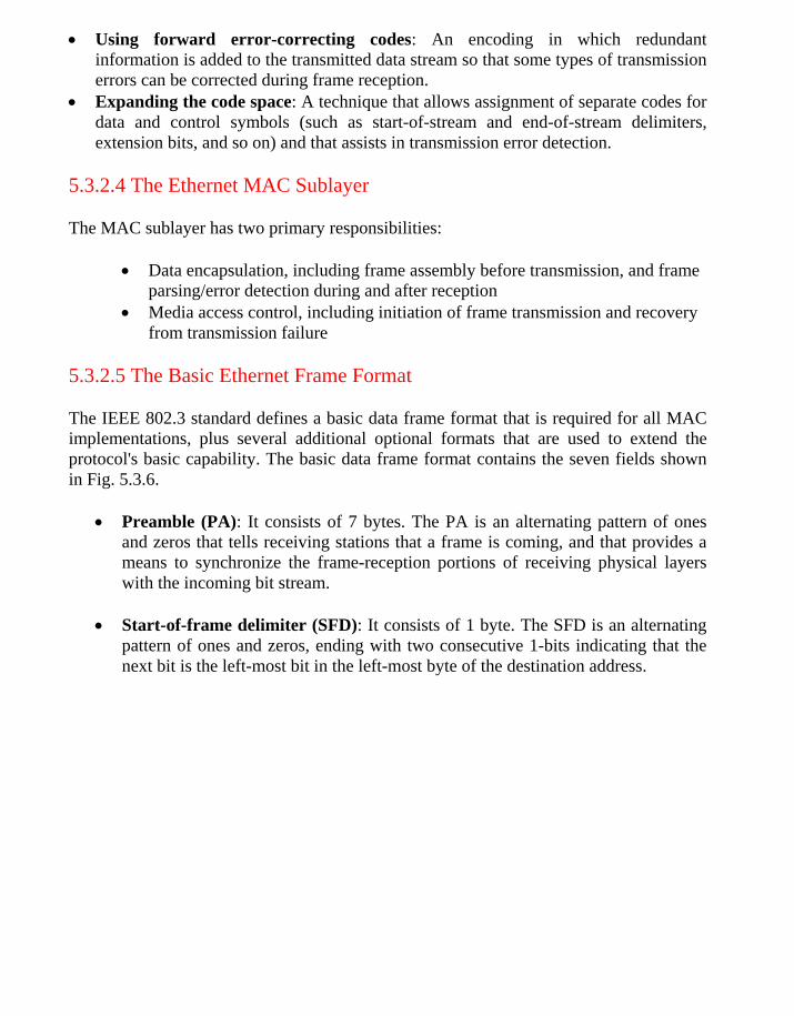
• Using forward error-correcting codes: An encoding in which redundant information is added to the transmitted data stream so that some types of transmission errors can be corrected during frame reception.

smission error detection.

The MAC sublayer has two primary responsibilities:

• Data encapsulation, including frame assembly before transmission, and frame eption

• Media access control, including initiation of frame transmission and recovery

The IEEE 802.3 standard defines a basic data frame format that is required for all MAC al formats that are used to extend the

protocol's basic capability. The basic data frame format contains the seven fields shown

os that tells receiving stations that a frame is coming, and that provides a means to synchronize the frame-reception portions of receiving physical layers

ing with two consecutive 1-bits indicating that the next bit is the left-most bit in the left-most byte of the destination address.

• Expanding the code space: A technique that allows assignment of separate codes for data and control symbols (such as start-of-stream and end-of-stream delimiters, extension bits, and so on) and that assists in tran

5.3.2.4 The Ethernet MAC Sublayer

parsing/error detection during and after rec

from transmission failure

5.3.2.5 The Basic Ethernet Frame Format

implementations, plus several additional option

in Fig. 5.3.6.

• Preamble (PA): It consists of 7 bytes. The PA is an alternating pattern of ones and zer

with the incoming bit stream.

• Start-of-frame delimiter (SFD): It consists of 1 byte. The SFD is an alternating pattern of ones and zeros, end


7 1 6 6 2 46-1500 4

6 6 2 4 8 46-1500

FCS PAD PA DA SA Type DATA

FCS PAD LLC PDU LEN SA DA PA SFD IEEE 802.3

Figure 5.3.6 Ethernet Frame Format

PA: Preamble --- 10101010s for synchronization SFD: Start of frame delimiter --- 10101011 to start frame DA: Destination MAC address SA: Source MAC address LEN: Length --- number of data bytes Type: Identify the higher-level protocol LLC PDU + Pad: minimum 46 bytes, maximum 1500 FCS: Frame Check Sequence --- CRC-32

• Destination address (DA): It onsists of 6 bytes. The DA field identifies which station(s) should receive the frame. The left-most bit in the DA field indicates whether the address is an individual address (indicated by a 0) or a group address (indicated by a 1). The second bit from the left indicates whether the DA is globally administered (indicated by a 0) or locally administered (indicated by a 1). The remaining 46 bits are a uniquely assigned value that identifies a single station, a defined group of stations, or all stations on the network as shown in Fig. 5.3.7..

I/G = 0 in case of individual address = 1 in case of group address U/L = 0 in case of global administered address = 1 in case of local administered address Unicast: Defines a single destination

Broadcast: FFFFFFFFFFFF each station on the network receive and accept frames Multicast: A group address defines multiple recipient Figure 5.3.7 Ethernet MAC Address

• Source addresses (SA): It consists of 6 bytes. The SA field identifies the sending station. The SA is always an individual address and the left-most bit in the SA field is always 0.


• Length/Type: It consists of 4 bytes. This field indicates either the number of MAC-client data bytes that are contained in the data field of the frame, or the frame type ID if the frame is assembled using an optional format. If the Length/Type field value is less than or equal to 1500, the number of LLC bytes in the Data field is equal to the Length/Type field value. If the Length/Type field value is greater than 1536, the frame is an optional type frame, and the Length/Type field value identifies the particular type of frame being sent or received.

• Data: It is a sequence of n bytes of any value, where n is less than or equal to 1500. If the length of the Data field is less than 46, the Data field must be extended by adding a filler (a pad) sufficient to bring the Data field length to 46 bytes.

• Frame check sequence (FCS): It consists of 4 bytes. This sequence contains a 32-bit cyclic redundancy check (CRC) value, which is created by the sending MAC and is recalculated by the receiving MAC to check for damaged frames. The FCS is generated over the DA, SA, Length/Type, and Data fields.

5.3.2.6 Other important issues There are some more important issues, which are briefly discussed below. • Inter-frame Gap: There is mandatory requirement of 9.6 ms interval between two

frames to enable other stations wishing to transmit to take over after a frame transmission is over. In other words, a 96 bit-time delay is provided between frame transmissions.

• How are collisions detected? A station sends frame and continues to sense the

medium. If the signal strength sensed by a station exceeds the normal signal strength, it is treated as collision detection.

• What the station does? The transmitting station sends a jamming signal after

collision is detected. 32-bit jam signal: 10101010 --- 10101010 48-bit jam signal: 10101010 --- 10101010

The jam signal serves as a mechanism to cause non-transmitting stations to wait until the jam signal ends. • Minimum Frame Size: A frame must take more than 2τ time to send, where τ is the

propagation time for preventing the situation that the sender incorrectly concludes that the frame was successfully sent. This slot time is 51.2μsec corresponding to 512 bit = 64 bytes. Therefore the minimum frame length is 64 bytes (excluding preamble), which requires that the data field must have a minimum size of 46 bytes.


Fill In The Blanks 1. The 802.2 standard describes the ____________, which is the upper part of the

data link layer. 2. LLC offers three types services: Unreliable datagram service,

________________ and _______________. 3. IEEE 802 bundle also includes a MAN standard IEEE 802.6 which is also known

as ______________. 4. 100Base-T2 means _______________________________ 5. 100 Mbps, baseband, long wavelength over optical fiber cable will be abbreviated

as ________________ 6. Ethernet uses __________ encoding

Answers: 1. LLC (logical link layer) 2. Acknowledged datagram service, Reliable connection oriental service 3. Distributed Queue Dual Bus (DQDB) 4. 100 Mbps, baseband, over two twisted-pair cables 5. 1000Base F 6. Bi-phase Manchester

Short question Answers

Q-1 What are the goals in mind of IEEE 802 committee? Ans: IEEE 802 committee has few goals in mind, namely

– To promote compatibility – Implementation with minimum efforts – Accommodate diverse applications

Q-2. List the functions performed by the physical layer of 802.3 standard? Ans. Functions of physical layer are:

i) Data encoding/decoding (To facilitate synchronization and efficient transfer of signal through the medium).

ii) Collision detection (It detects at the transmit side) iii) Carrier sensing (Channel access senses a carrier on the channel at both the

transmit and receive sides) iv) Transmit/receive the packets (Frame transmitted to all stations connected

to the channel) v) Topology and medium used (Mediums are co-axial cable, twisted pair and

fiber optic cable) Q-3. Why do you require a limit on the minimum size of Ethernet frame? Ans. To detect collision, it is essential that a sender continue sending a frame and at the same time receives another frame sent by another station. Considering maximum delay


with five Ethernet segments in cascade, the size of frame has been found to be 64 bytes such that the above condition is satisfied. Q-4. What are the different types of cabling supported by Ethernet standard? Ans. Types of cabling are:

i) 10 BASE 5 - Maximum cable length is 500 meters using 4” diameter coaxial cable.

ii) 10 BASE 2 - Maximum cable length is 185 meters using 0.25” diameter CATV cable.

iii) 10 BASE T - Maximum cable length is 100 meters using twisted-pair cable (CAT-3 UTP).

iv) 10 BASE FL - Maximum cable length is 2 Km using multimode fiber optic cable (125/62.5 micrometer).


Specific Instructional Objectives At the end of this lesson, the students will become familiar with the following concepts:

• Explain the operation of IEEE 802 LANs

o 802.4 – Token bus-based o 802.5 – Token ring-based

• Compare performance of the three LANs 5.4.1 Introduction In the preceding lesson we have mentioned that for the fulfillment of different goals, the IEEE 802 committee came up with a bunch of LAN standards collectively known as LANs as shown in Fig. 5.4.1. We have already discussed CSMA/CD-based LAN proposed by the IEEE 802.3 subcommittee, commonly known as Ethernet. In this lesson we shall discuss Token bus, Token Ring based LANs proposed by the IEEE 802.4 and IEEE 8.2.5 subcommittees.

Figure 5.4.1 IEEE 802 Legacy LANs 5.4.2 Token Ring (IEEE 802.5)

5.4.2.1 Token Ring: A Brief History

Originally, IBM developed Token Ring network in the 1970s. It is still IBM's primary local-area network (LAN) technology. The related IEEE 802.5 specification is almost identical to and completely compatible with IBM's Token Ring network. In fact, the IEEE 802.5 specification was modeled after IBM Token Ring, and on the same lines. The term Token Ring is generally used to refer to both IBM's Token Ring network and IEEE 802.5 networks.


5.4.2.2 Introduction Before going into the details of the Token Ring protocol, let’s first discuss the motivation behind it. As already discussed, the medium access mechanism used by Ethernet (CSMA/CD) may results in collision. Nodes attempt to a number of times before they can actually transmit, and even when they start transmitting there are chances to encounter collisions and entire transmission need to be repeated. And all this become worse one the traffic is heavy i.e. all nodes have some data to transmit. Apart from this there is no way to predict either the occurrence of collision or delays produced by multiple stations attempting to capture the link at the same time. So all these problems with the Ethernet gives way to an alternate LAN technology, Token Ring.

Token Ring and IEEE802.5 are based on token passing MAC protocol with ring topology. They resolve the uncertainty by giving each station a turn on by one. Each node takes turns sending the data; each station may transmit data during its turn. The technique that coordinates this turn mechanism is called Token passing; as a Token is passed in the network and the station that gets the token can only transmit. As one node transmits at a time, there is no chance of collision. We shall discuss the detailed operation in next section.

Stations are connected by point-to-point links using repeaters. Mainly these links are of shielded twisted-pair cables. The repeaters function in two basic modes: Listen mode, Transmit mode. A disadvantage of this topology is that it is vulnerable to link or station failure. But a few measures can be taken to take care of it.

Differences between Token Ring and IEEE 802.5 Both of these networks are basically compatible, although the specifications differ in some ways. • IEEE 802.5 does not specify a topology, although virtually all IEEE 802.5

implementations are based on the star topology. While IBM's Token Ring network explicitly specifies a star, with all end stations attached to a device called a Multi-Station Access Unit (MSAU).

• IEEE 802.5 does not specify a media type, although IBM Token Ring networks use twisted-pair wire.

• There are few differences in routing information field size of the two.

5.4.2.3 Token Ring Operation Token-passing networks move a small frame, called a token, around the network. Possession of the token grants the right to transmit. If a node receiving the token has no information to send, it passes the token to the next end station. Each station can hold the token for a maximum period of time.


If a station possessing the token does have information to transmit, it seizes the token, alters 1 bit of the token (which turns the token into a start-of-frame sequence), appends the information that it wants to transmit, and sends this information to the next station on the ring. While the information frame is circling the ring, no token is on the network (unless the ring supports early token release), which means that other stations wanting to transmit must wait. Therefore, collisions cannot occur in Token Ring networks. If early token release is supported, a new token can be released immediately after a frame transmission is complete.

The information frame circulates around the ring until it reaches the intended destination station, which copies the information for further processing. The information frame makes a round trip and is finally removed when it reaches the sending station. The sending station can check the returning frame to see whether the frame was seen and subsequently copied by the destination station in error-free form. Then the sending station inserts a new free token on the ring, if it has finished transmission of its packets.

Unlike CSMA/CD networks (such as Ethernet), token-passing networks are deterministic, which means that it is possible to calculate the maximum time that will pass before any end station will be capable of transmitting. Token Ring networks are ideal for applications in which delay must be predictable and robust network operation is important.

5.4.2.4 Priority System Token Ring networks use a sophisticated priority system that permits certain user-designated, high-priority stations to use the network more frequently. Token Ring frames have two fields that control priority: the priority field and the reservation field.

Only stations with a priority equal to or higher than the priority value contained in a token can seize that token. After the token is seized and changed to an information frame, only stations with a priority value higher than that of the transmitting station can reserve the token for the next pass around the network. When the next token is generated, it includes the higher priority of the reserving station. Stations that raise a token's priority level must reinstate the previous priority after their transmission is complete.

5.4.2.5 Ring Maintenance There are two error conditions that could cause the token ring to break down. One is the lost token in which case there is no token the ring, the other is the busy token that circulates endlessly. To overcome these problems, the IEEE 802 standard specifies that one of the stations be designated as ‘active monitor’. The monitor detects the lost condition using a timer by time-out mechanism and recovers by using a new free token. To detect a circulating busy token, the monitor sets a ‘monitor bit’ to one on any passing busy token. If it detects a busy token with the monitor bit already set, it implies that the sending station has failed to remove its packet and recovers by changing the busy token to a free token. Other stations on the ring have the role of passive monitor. The primary


job of these stations is to detect failure of the active monitor and assume the role of active monitor. A contention-resolution is used to determine which station to take over.

5.4.2.6 Physical Layer The Token Ring uses shielded twisted pair of wire to establish point-point links between the adjacent stations. The baseband signaling uses differential Manchester encoding. To overcome the problem of cable break or network failure, which brings the entire network down, one suggested technique, is to use wiring concentrator as shown in Fig. 5.4.2.

Figure 5.4.2 Star Connected Ring topology

It imposes the reliability in an elegant manner. Although logically the network remains as a ring, physically each station is connected to the wire center with two twisted pairs for 2-way communication. Inside the wire center, bypass relays are used to isolate a broken wire or a faulty station. This Topology is known as Star-Connected Ring.

5.4.2.7 Frame Format Token Ring and IEEE 802.5 support two basic frame types: tokens and data/command frames. Tokens are 3 bytes in length and consist of a start delimiter, an access control byte, and an end delimiter. Data/command frames vary in size, depending on the size of the Information field. Data frames carry information for upper-layer protocols, while command frames contain control information and have no data for upper-layer protocols.

Token Frame Fields Start Delimiter Access Control Ending delimiter

Token Frame contains three fields, each of which is 1 byte in length:


• Start delimiter (1 byte): Alerts each station of the arrival of a token (or data/command frame). This field includes signals that distinguish the byte from the rest of the frame by violating the encoding scheme used elsewhere in the frame.

• Access-control (1 byte): Contains the Priority field (the most significant 3 bits) and the Reservation field (the least significant 3 bits), as well as a token bit (used to differentiate a token from a data/command frame) and a monitor bit (used by the active monitor to determine whether a frame is circling the ring endlessly).

• End delimiter (1 byte): Signals the end of the token or data/command frame. This field also contains bits to indicate a damaged frame and identify the frame that is the last in a logical sequence.

Data/Command Frame Fields Start Delimiter

Access Control

Frame Control

Destination address

Source address

Data Frame check sequence

End Delimiter

Frame Status

Data/command frames have the same three fields as Token Frames, plus several others. The Data/command frame fields are described below:

• Frame-control byte (1 byte)—Indicates whether the frame contains data or control information. In control frames, this byte specifies the type of control information.

• Destination and source addresses (2-6 bytes)—Consists of two 6-byte address fields that identify the destination and source station addresses.

• Data (up to 4500 bytes)—Indicates that the length of field is limited by the ring token holding time, which defines the maximum time a station can hold the token.

• Frame-check sequence (FCS- 4 byte)—Is filed by the source station with a calculated value dependent on the frame contents. The destination station recalculates the value to determine whether the frame was damaged in transit. If so, the frame is discarded.

• Frame Status (1 byte)—This is the terminating field of a command/data frame. The Frame Status field includes the address-recognized indicator and frame-copied indicator.

5.4.3 Token Bus (IEEE 802.4) 5.4.3.1 Token BUS: A Brief History Although Ethernet was widely used in the offices, but people interested in factory automation did not like it because of the probabilistic MAC layer protocol. They wanted a protocol which can support priorities and has predictable delay. These people liked the conceptual idea of Token Ring network but did not like its physical implementation as a break in the ring cable could bring the whole network down and ring is a poor fit to their linear assembly lines. Thus a new standard, known as Token bus, was developed, having the robustness of the Bus topology, but the known worst-case behavior of a ring. Here


stations are logically connected as a ring but physically on a Bus and follows the collision-free token passing medium access control protocol. So the motivation behind token bus protocol can be summarized as:

• The probabilistic nature of CSMA/ CD leads to uncertainty about the delivery time; which created the need for a different protocol

• The token ring, on the hand, is very vulnerable to failure. • Token bus provides deterministic delivery time, which is necessary for real time

traffic. • Token bus is also less vulnerable compared to token ring.

5.4.3.2 Functions of a Token Bus It is the technique in which the station on bus or tree forms a logical ring, that is the stations are assigned positions in an ordered sequence, with the last number of the sequence followed by the first one as shown in Fig. 5.4.3. Each station knows the identity of the station following it and preceding it.

Figure 5.4.3 Token Bus topology

A control packet known as a Token regulates the right to access. When a station receives the token, it is granted control to the media for a specified time, during which it may transmit one or more packets and may poll stations and receive responses when the station is done, or if its time has expired then it passes token to next station in logical sequence. Hence, steady phase consists of alternate phases of token passing and data transfer.

The MAC sublayer consists of four major functions: the interface machine (IFM), the

access control machine (ACM), the receiver machine (RxM) and the transmit machine (TxM).

IFM interfaces with the LLC sublayer. The LLC sublayer frames are passed on to the

ACM by the IFM and if the received frame is also an LLC type, it is passed from RxM component to the LLC sublayer. IFM also provides quality of service.

The ACM is the heart of the system. It determines when to place a frame on the bus,

and responsible for the maintenance of the logical ring including the error detection and fault recovery. It also cooperates with other stations ACM’s to control the access to the


shared bus, controls the admission of new stations and attempts recovery from faults and failures.

The responsibility of a TxM is to transmit frame to physical layer. It accepts the

frame from the ACM and builds a MAC protocol data unit (PDU) as per the format. The RxM accepts data from the physical layer and identifies a full frame by detecting

the SD and ED (start and end delimiter). It also checks the FCS field to validate an error-free transmission.

5.4.3.3 Frame Form The frame format of the Token Bus is shown in Fig. 5.4.4. Most of the fields are same as Token Ring. So, we shall just look at the Frame Control Field in Table 5.4.1

Figure 5.4.4 Token Bus frame format

Table 5.4.1 The Frame Control Field

Frame Control Name Use 0000 0000 Claim-Token Ring Initialization 0000 0001 Solicit-successor -1 Addition to the Ring 0000 0010 Solicit-successor -2 Addition to the Ring 0000 0011 Who-follows Recovery from lost token 0000 0100 Resolve Contention Multiple station to join the Ring 0000 1000 Token Pass the Token 0000 1100 Set-Successor Deletion from the ring

5.4.3.4 Logical ring maintenance The MAC performs the following functions as part of its maintenance role of the ring. Addition to the Ring: Non-participating stations must periodically be granted the opportunity to insert themselves into the ring. Each node in the ring periodically grants an opportunity for new nodes to enter the ring while holding the token. The node issues a solicit–successor–1 packet, inviting nodes with an address between itself and the next


node in logical sequence to request entrance. The transmitting node then waits for a period of time equal to one response window or slot time (twice the end-to-end propagation delay of the medium). If there is no request, the token holder sets its successor node to be the requesting node and transmits the token to it; the requester sets the linkages accordingly and proceeds.

If more than one node requests, to enter the ring, the token holder will detect a garbled transmission. The conflict is resolved by addressed based contention scheme; the token holder transmits a resolved contention packet and waits for four response windows. Each requester can transmit in one of these windows, based on the first two bits of its address. If requester hears anything before its windows comes up, it refrains from requesting entrance. If a token holder receives a valid response, then it can proceed, otherwise it tries again and only those nodes that request the first time are allowed to request this time, based on the second pair of bits in their address. This process continues until a valid request is received or no request is received, or a maximum retry count is reached. In latter cases, the token holder passes the token to logical successor in the ring.

Deletion from Ring: A station can voluntarily remove itself from the ring by splicing together its predecessor and successor. The node which wants to be deleted from the ring waits until token comes to it, then it sends a set successor packet to its predecessor, instructing it to splice to its successor.

Fault Management: Errors like duplicate address or broken ring can occur. A suitable management scheme should be implemented for smooth functioning. It is done by the token-holder first, while holding the token, node may hear a packet, indicating that another node has the token. In this case, it immediately drops the token by reverting to listener mode, and the number of token holders drops immediately from one to zero. Upon completion of its turn, it immediately issues a data or token packet. The sequence of steps are as follows:

i. After sending the token, the token issuer will listen for one slot time to make sure that its predecessor is active.

ii. If the issuer does not hear a valid packet, it reissues the token to the same successor one more time.

iii. After two failures, the issuer assumes that its successor has failed and issues a “who-follows” packet, asking for the identity of the node that follows the failed node. The issuer should get back a set successor packet from the second node down the time. If so, the issuer adjusts its linkage and issues a token (back to step i).

iv. If the issuing node gets a response to its “who-follows” packet, it tries again. v. If the “who-follows” tactic fails, the node issues a solicit-successor-2 packet

with full address range (i.e. every node is invited to respond). If this packet works then the ring is established and procedure continues.

vi. If two attempts in step (v) fail, it assumes that a catastrophe has happened; perhaps the node receiver has failed. In any case, the node ceases the activity and listen the bus.


Ring Initialization: Ring is to be initialized by starting the token passing. This is necessary when the network is being setup or when ring is broken down. Some decentralized algorithms should take care of, who starts first, who starts second, etc. it occurs when one or more stations detects a lack of bus activity lasting longer than a specific time. The token may get lost. This can occur on a number of occasions. For example, when network has been just powered up, or a token holding station fails. Once its time out expires, a node will issue a claim token packet. Contending clients are removed in a similar fashion to the response window process. 5.4.3.4 Relative comparison of the three standards A comparison of the three standards for different functions is shown in Table 5.4.2 and results of the analysis of the performance of the three standards are summarized below:

• The CSMA/CD protocol shows strong dependence on the parameter ‘a’, which is the ratio of the propagation time to the transmission time. It offers shortest delay under light load and it is most sensitive under heavy load conditions.

• Token ring is least sensitive to different load conditions and different packet sizes.

• Token bus is highly efficient under light load conditions.

Table 5.4.2 Comparison of the three standards

Function CSMA/CD Token bus Token ring Access determination Contention Token Token

Packet length restriction

64 bytes (Greater than 2.Tprop)

None None

Priority Not supported Supported Supported Sensitivity to work load Most sensitive Sensitive Least sensitive

Principle advantage Simplicity, wide installed base

Regulated/fair access

Regulated/fair access

Principle disadvantage Nondeterministic delay

Complexity Complexity

Fill In The Blanks

1. Originally, ______________ developed Token Ring network in the ________. 2. A disadvantage of this topology is that it is vulnerable to _________ or _____

failure. 3. Unlike CSMA/CD networks (such as Ethernet), token-passing networks are

________________, which means that it is possible to calculate the maximum time that will pass before any end station will be capable of transmitting.

4. Token Ring frames have two fields that control priority: ___________ and the ___________field.


5. In Token Ring inside the wire center, _____________ are used to isolate a broken wire or a faulty station.

6. The Mac sublayer in Token BUS consists of four major functions: ____________, the access control machine (ACM), ______________________and ____________.

7. ___________ determines when to place a frame on the bus, and responsible for the maintenance of the logical ring including the error detection and fault recovery.

Answers:

1. IBM, 1970 2. link, station 3. deterministic 4. the priority field, reservation 5. bypass relays 6. the interface machine (IFM), the receiver machine (RxM), the transmit machine

(TxM). 7. Access control machine (ACM)

Short question Answers: Q-1. What is the advantage of token passing protocol over CSMA/CD protocol? Ans. Advantage of token passing protocol over CSMA/CD protocol:

The CSMA/CD is not a deterministic protocol. A packet may be delivered after many (up to 15) collisions leading to long variable delay. An unfortunate packet may not get delivered at all. This feature makes CSMA/CD protocol unsuitable for real-time applications. On the other hand, token passing protocol is a deterministic approach, which allows a packet to be delivered within a known time frame. It also allows priority to be assigned to packets. These are the two key advantages of token passing protocol over CSMA/CD protocol.

Q-2. What are the drawbacks of token ring topology? Ans. Token ring protocol cannot work if a link or a station fails. So, it is vulnerable to link and station failure. Q-3. How the reliability of token ring topology can be improved? Ans. Reliability of the ring network can be improved by implementing the ring topology using a wiring concentrator. This allows not only to detect fault, but also to isolate the faulty link/station with the help of a bypass relay. Q-4. What role the active token monitor performs? Ans. Token ring is maintained with the help of active token monitor. Any one of the stations has the capability to act as active token monitor, but at a particular instant only


one acts as active token monitor. It monitors various error situations such as multiple token, orphan packet, etc, and takes appropriate action to come out of the error situation.


Specific Instructional Objectives On completion, the student will be able to:

• Explain the need for wireless LAN • Identify the limitations and challenges of wireless LAN • Understand different aspects of IEEE 802.11 WLAN

o Transmission media o Topology o Medium Access Control o Security

5.7.1 Introduction In the last two decades the wired version of LAN has gained wide popularity and large-scale deployment. The IEEE 802.3 standard has been revised and extended every few years. High-speed versions with transmission rate as high as 1000 Mbps are currently available. Until recently wireless version of LANs were not popular because of the following reasons:

• High cost: Previously the equipments cost more. • Low data rate: Initially, the data rate supported by the WLAN is too less, so

it supports only a few applications. • Occupational safety concerns • Licensing requirements

In the last couple of years the situation has changed significantly. Cheaper, smaller and powerful notebook computers and other mobile computing equipment have proliferated in homes and offices. These devices share various resources such as printers, files and Broadband Internet connections. This has opened up the need for wireless LAN. Wireless LANs also offer a number of other advantages compared to their wired counterpart. Before going into the technical details of Wireless LAN let us first look at various reasons which have led to the development of WLANs. Some of the advantages are mentioned below:

• Availability of low-cost portable equipments: Due to the technology enhancements, the equipment cost that are required for WLAN set-up have reduced a lot.

• Mobility: An increasing number of LAN users are becoming mobile. These mobile users require that they are connected to the network regardless of where they are because they want simultaneous access to the network. This makes the use of cables, or wired LANs, impractical if not impossible. Wireless LAN can provide users mobility, which is likely to increase productivity, user convenience and various service opportunities.

• Installation speed and simplicity: Wireless LANs are very easy to install. There is no requirement for wiring every workstation and every room. This ease of installation makes wireless LANs inherently flexible. If a workstation must be


moved, it can be done easily and without additional wiring, cable drops or reconfiguration of the network.

• Installation flexibility: If a company moves to a new location, the wireless system is much easier to move than ripping up all of the cables that a wired system would have snaked throughout the building. This also provides portability. Wireless technology allows network to go anywhere wire cannot reach.

• Reduced cost of ownership: While the initial cost of wireless LAN can be higher than the cost of wired LAN hardware, it is envisaged that the overall installation expenses and life cycle costs can be significantly lower. Long-term cost-benefits are greater in dynamic environment requiring frequent moves and changes.

• Scalability: Wireless LAN can be configured in a variety of topologies to meet the users need and can be easily scaled to cover a large area with thousands of users roaming within it.

However, wireless LAN technology needs to overcome a number of inherent limitations and challenges. Some of the limitations and challenges are mentioned below: • Lower reliability due to susceptibility of radio transmission to noise and

interference. • Fluctuation of the strength of the received signal through multiple paths causing

fading. • Vulnerable to eavesdropping leading to security problem. • Limited data rate because of the use of spread spectrum transmission techniques

enforced to ISM band users. In this lesson we shall introduce the wireless LAN technology based on IEEE 802.11 standard. Its predecessor the IEEE 802.3, commonly referred to as the Ethernet, is the most widely deployed member of the family. IEEE 802.11 is commonly referred to as wireless Ethernet because of its close similarity with the IEEE 802.3. Like IEEE 802.3, it also defines only two bottom levels of ISO’s open system Interconnection (OSI) model as shown in Fig. 5.7.1. As it shares the upper layers with other LAN standards, it is relatively easy to bridge the IEEE 802.11 wireless LANs to other IEEE 802.11 wired LANs to form an extended interconnected wired and wireless LAN network. Although initially wireless LANs were perceived to be as a substitute to wired LANs, now it is recognized as an indispensable adjunct to wired LANs.


Application Layer

Presentation Layer

Session Layer Network

Operating System

(NOS)

TCP

IP

Transport Layer

Network Layer

OSI IEEE 802.11

Figure 5.7.1 OSI Reference Model and IEEE 802.11

The IEEE 802.11 standard basically defines the physical and data link layer. In the later sections we shall look at detailed implementations. 5.7.2 Transmission Media There are three media that can be used for transmission over wireless LANs. Infrared, radio frequency and microwave. In 1985 the United States released the industrial, scientific, and medical (ISM) frequency bands. These bands are 902 - 928MHz, 2.4 - 2.4853 GHz, and 5.725 - 5.85 GHz and do not require licensing by the Federal Communications Commission (FCC). This prompted most of the wireless LAN products to operate within ISM bands. The FCC did put restrictions on the ISM bands however. In the U.S. radio frequency (RF) systems must implement spread spectrum technology. RF systems must confine the emitted spectrum to a band. RF is also limited to one watt of power. Microwave systems are considered very low power systems and must operate at 500 milliwatts or less. 5.7.2.1 Infrared Infrared systems (IR systems) are simple in design and therefore inexpensive. They use the same signal frequencies used on fiber optic links. IR systems detect only the amplitude of the signal and so interference is greatly reduced. These systems are not bandwidth limited and thus can achieve transmission speeds greater than the other systems. Infrared transmission operates in the light spectrum and does not require a license from the FCC to operate. There are two conventional ways to set up an IR LAN.

Logical Link Layer (LLC) 802.2 Data Link Layer 802.11b Medium Access Control (MAC) Physical Layer


The infrared transmissions can be aimed. This gives a good range of a couple of kilometer and can be used outdoors. It also offers the highest bandwidth and throughput.

The other way is to transmit omni-directionally and bounce the signals off of everything in every direction. This reduces coverage to 30 - 60 feet, but it is area coverage. IR technology was initially very popular because it delivered high data rates and relatively cheap price.

The drawbacks to IR systems are that the transmission spectrum is shared with the sun and other things such as fluorescent lights. If there is enough interference from other sources it can render the LAN useless. IR systems require an unobstructed line of sight (LOS). IR signals cannot penetrate opaque objects. This means that walls, dividers, curtains, or even fog can obstruct the signal. InfraLAN is an example of wireless LANs using infrared technology.

5.7.2.2 Microwave Microwave (MW) systems operate at less than 500 milliwatts of power in compliance with FCC regulations. MW systems are by far the fewest on the market. They use narrow-band transmission with single frequency modulation and are set up mostly in the 5.8GHz band. The big advantage to MW systems is higher throughput achieved because they do not have the overhead involved with spread spectrum systems. RadioLAN is an example of systems with microwave technology. 5.7.2.3 Radio Radio frequency systems must use spread spectrum technology in the United States. This spread spectrum technology currently comes in two types: direct sequence spread spectrum (DSSS) and frequency hopping spread spectrum (FHSS). There is a lot of overhead involved with spread spectrum and so most of the DSSS and FHSS systems have historically had lower data rates than IR or MW.

Direct Sequence Spread Spectrum (DSSS) Scheme Direct Sequence Spread Spectrum (DSSS) represents each bit in the frame by multiple bits in the transmitted frame. DSSS represents each data 0 and 1 by the symbol –1 and +1 and then multiplies each symbol by a binary pattern of +1’s and –1’s to obtain a digital signal that varies more rapidly occupying larger band. The IEEE 802.11 uses a simple 11-chip Barker sequence B11 [-1, +1, -1, -1, +1, -1, -1, -1, +1, +1, +1] with QPSK or BPSK modulation as shown in Figure 5.7.2. The DSSS transmission system takes 1 Mbps data, converts it into 11 Mbps signal using differential binary phase shift keying (DBPSK) modulation.

The Barker sequence provides good immunity against interference and noise as well as some protection against multi-path propagation. In both cases of spread spectrum transmission, the signal look like noise to any receiver that does not know the pseudorandom sequence. The third transmission media is based on infrared signal in the near visible range of 850 to 950 nanometers. Diffused transmission is used so that the


transmitter and receivers do not have to point to each other and do not require a clear line of sight communication. The transmission distance is limited to 10 to 20 meters and is limited to inside the buildings only.

Figure 5.7.2 Direct-sequence spread spectrum technique using Barker sequence

With direct sequence spread spectrum the transmission signal is spread over an allowed band (for example 25MHz). A random binary string is used to modulate the transmitted signal. This random string is called the spreading code. The data bits are mapped to into a pattern of "chips" and mapped back into a bit at the destination. The number of chips that represent a bit is the spreading ratio. The higher the spreading ratio, the more the signal is resistant to interference. The lower the spreading ratio, the more bandwidth is available to the user. The FCC dictates that the spreading ratio must be more than ten. Most products have a spreading ratio of less than 20 and the new IEEE 802.11 standard requires a spreading ratio of eleven. The transmitter and the receiver must be synchronized with the same spreading code. If orthogonal spreading codes are used then more than one LAN can share the same band. However, because DSSS systems use wide sub channels, the number of co-located LANs is limited by the size of those sub channels. Recovery is faster in DSSS systems because of the ability to spread the signal over a wider band. Current DSSS products include Digital's RoamAbout and NCR's WaveLAN.

Figure 5.7.3 shows a typical DSSS implementation. Here, the data stream and pseudo-random sequence are both converted into analog signals before combining, rather than performing the exclusive-OR of the two streams and than modulating. Eleven channels have been defined to operate in the 2.4 GHz ISM band in US. Channels can operate without interference with each other if their center frequencies are separated by at least 30MHz. The 802.11 DSSS physical layer also defines an option for 2 Mbps operation using Differential Quadrature PSK (DQPSK).

+1-1

+1 +1-1 -1

+1 +1 +1-1 -1

(a) 11-chip Barker sequence

+1-1

+1 +1-1 -1

+1 +1 +1-1 -1

(b) Transmission of -1

-1 -1 -1+1 +1 +1

-1 -1+1 +1

-1

(c) Transmission of +1


(a) Transmitter (b) Receiver

Figure 5.7.3 Direct Sequence Spread Spectrum (DSSS) system,

Frequency Hopping Spread Spectrum (FHSS)

The idea behind spread spectrum is to spread the signal over a wider frequency band, so as to make jamming and interception more difficult and to minimize the effect of interference from other devices In FH it is done by transmitting the signal over a random sequence of frequencies; that is, first transmitting at one frequency, then second, then a third and so on. The random sequence of frequencies is generated with the help of a pseudorandom number generator. As both the receiver and sender use the same algorithm to generate random sequence, both the devices hop frequencies in a synchronous manner and frames transmitted by the sender are received correctly by the receiver. This is somewhat similar to sending different parts of one song over several FM channels. Eavesdroppers hear only unintelligible blips and any attempt to jam the signal results in damaging a few bits only.

Typical block diagram of a frequency-hopping system is shown in Figure 5.7.4. As shown in Figure 5.7.4(a) the digital data is first encoded to analog signal, such as frequency-shift keying (FSK) or Binary-phase shift keying (BPSK). At any particular instant, a carrier frequency is selected by the pseudo-random sequence. The carrier frequency is modulated by the encoder output a then transmitted after band pass filtering At the receiving end, the spread-spectrum signal is demodulated using the same sequence of carrier frequencies generated with the help of same pseudo-random sequence in synchronization with the transmitter, and the demodulated signal filtered using a band-pass filter before decoding as shown in Fig. 5.7.4(b).


This technique splits the band into many small sub channels (each of 1MHz). The signal then hops from sub channel to sub channel transmitting short bursts of data on each channel for a set period of time, called dwell time. The hopping sequence must be synchronized at the sender and the receiver or information is lost.

The 802.11 frequency hopping physical layer uses 79 non-overlapping 1 MHz

Channels to transmit 1 Mbps data signal over 2.4 GHz ISM band. There is option to transmit at the rate of 2 Mbps. A channel hop occurs every 224 μsec. The standard defines 78 hopping patterns that are divided into three sets of 26 patterns each. Each hopping pattern jumps a minimum of six channels in each hop and the hopping sequences are derived via a simple modulo 79 calculation. The hopping patterns from each set collide three times on the average and five times in the worst case over a hopping cycle. Each 802.11 network must use a particular hopping pattern. The hopping patterns allow up to 26 networks to be collocated and still operate simultaneously.

Figure 5.7.4 Frequency Hopping system, (a) Transmitter (b) Receiver

This feature gives FH systems a high degree of security. In order to jam a frequency hopping system the whole band must be jammed. These features are very attractive to agencies involved with law enforcement or the military. Many FHSS LANs can be co-located if an orthogonal hopping sequence is used. Because the sub channels are smaller than in DSSS, the number of co-located LANs can be greater with FHSS systems. Most new products in wireless LAN technology are currently being developed


with FHSS technology. Some examples are WaveAccess's Jaguar, Proxim RangeLAN2, and BreezeCom's BreezeNet Pro.

Multipath Interference

Interference caused by signals bouncing off of walls and other barriers and arriving at the receiver at different times is called multipath interference. Multipath interference affects IR, RF, and MW systems. FHSS inherently solves the multipath problem by simply hopping to other frequencies. Other systems use anti-multipath algorithms to avoid this interference. A subset of multipath is Rayleigh fading. This occurs when the difference in path length is arriving from different directions and is a multiple of half the wavelength. Rayleigh fading has the effect of completely cancelling out the signal. IR systems are not affected by Rayleigh fading, because the wavelengths used in IR are very small.

5.7.3 Topology Each computer, mobile, portable or fixed, is referred to as a station in 802.11. The difference between a portable and mobile station is that a portable station moves from point to point but is only used at a fixed point. Mobile stations access the LAN during movement. Fundamental to the IEEE 802.11 architecture is the concept of Basic Service Set (BSS) or wireless LAN cell. A BSS is defined as a group of stations that coordinate their access to the medium under a given instance of medium access control. The geographic area covered by a BSS is known as the Basic Service Area (BSA), which is very similar to a cell in a cellular communication network. All stations with in a BSA with tens of meters in diameter may communicate with each other directly. The 802.11 standard support the formation of two distinct types of BSSs: ad hoc network and Infrastructure BSS.

Two or more BSS's are interconnected using a Distribution System or DS. This concept of DS increases network coverage. Each BSS becomes a component of an extended, larger network. Entry to the DS is accomplished with the use of Access Points (AP). An access point is a station, thus addressable. So data moves between the BSS and the DS with the help of these access points.

Creating large and complex networks using BSS's and DS's leads us to the next

level of hierarchy, the Extended Service Set or ESS. The beauty of the ESS is the entire network looks like an independent basic service set to the Logical Link Control layer (LLC). This means that stations within the ESS can communicate or even move between BSS's transparently to the LLC.

The first type of BSS is known as ad hoc network, which consists of a group of

stations within the range of each other. As its name implies, ad hoc networks are temporary in nature, which are typically created and maintained as needed without prior administrative arrangement. Ad hoc networks can be formed anywhere spontaneously and can be disbanded after a limited period of time. A typical ad hoc network is shown in Figure 5.7.5(a).


The second type of BSS is known as infrastructure BSS (IBSS), which is

commonly used in practice. An ESS is shown in Fig. 5.7.6 Here, several BSSs are interconnected by a distribution system to form an extended service set (ESS) as shown in Fig. 5.7.5(b). The BSSs are like cells in a cellular communications network. Each BSS is provided with an Access point (AP) that has station functionality and provides access to the distribution system. APs operate on a fixed channel and remain stationary like base stations in a cellular communication system. APs are located such that the BSSs they serve overlap slightly to provide continuous service to all the stations.

(a) (b)

Figure 5.7.5 (a) Basic Service set (BSS), (b) Infrastructure BSS (ESS)

Figure 5.7.6 Extended service set (ESS) An ESS can also provide gateway access for wireless users into a wired network. Each end station associates itself with one access point. Figure 5.7.6 shows three BSSs interconnected through three APs to a distribution system. If station A associated with AP-1 wants to send a frame to another station associated with AP-2, the first sends a frame to its access point (AP-1), which forwards the frame across the distribution system


to the access point AP-2. AP-2 finally delivers it to the destination station. For forwarding frames across the APs, bridging protocol may be used, which is beyond the scope of IEEE 802.11 standard. However, the 802.11 standard specifies how stations select their access points. The technique used for this purpose is known as scanning, which involves the following steps:

• A station sends a probe frame. • All APs within reach reply with a probe response frame. • The station selects one of the access points, and sends the AP an Association

Request frame. • The AP replies with an Association Response frame. The above protocol is used when a station joins a network or when it wants to

discontinue association with the existing AP because of weakened signal strength or some other reason. The discontinuation of association takes place whenever a station acquires a new AP and the new AP announces it in step 4 mentioned above. For example, assume that station B is moving away from the BSS of AP-1 towards the BSS of AP-2. As it moves closer to the BSS of AP-2, it sends probe frames, which is responded eventually by AP-2. As some of point of time station B prefers AP-2 over AP-1 and associates itself with the access point AP-2. The above mechanism is known as active scanning, as the node is actively searching for an access point. An access point also periodically sends Beacon frame that advertises the capabilities of the access point. In response, a station can associate to the AP simply by sending it an Association request frame. This is known as passive scanning. 5.7.4 Medium Access Control Most wired LANs products use Carrier Sense Multiple Access with Collision Detection (CSMA/CD) as the MAC protocol. Carrier Sense means that the station will listen before it transmits. If there is already someone transmitting, then the station waits and tries again later. If no one is transmitting then the station goes ahead and sends what it has. But when more than one station tries to transmit, the transmissions will collide and the information will be lost. This is where Collision Detection comes into play. The station will listen to ensure that its transmission made it to the destination without collisions. If a collision occurred then the stations wait and try again later. The time the station waits is determined by the back off algorithm. This technique works great for wired LANs but wireless topologies can create a problem for CSMA/CD. However, the wireless medium presents some unique challenges not present in wired LANs that must be dealt with by the MAC used for IEEE 802.11. Some of the challenges are:

• The wireless LAN is prone to more interference and is less reliable. • The wireless LAN is susceptible to unwanted interception leading to security

problems. • There are so called hidden station and exposed station problems.


In the discussion of both the problem, we shall assume that all radio transmitters have fixed range. When the receiver is in the range of two active transmitters then the signal will be garbled. It is important to note that not all stations are in range of two transmitters. The Hidden Station Problem Consider a situation when A is transmitting to B, as depicted in the Fig. 5.7.7. If C senses the media, it will not hear anything because it is out of range, and thus will falsely conclude that no transmission is going on and will start transmit to B. the transmission will interfere at B, wiping out the frame from A. The problem of a station not been able to detect a potential competitor for the medium because the competitor is too far away is referred as Hidden Station Problem. As in the described scenario C act as a hidden station to A, which is also competing for the medium.

Error!

Figure 5.7.7 Hidden Station Problem

Exposed Station problem Now consider a different situation where B is transmitting to A, and C sense the medium and detects the ongoing transmission between B and A. C falsely conclude that it can not transmit to D, when the fact is that such transmission would cause on problem. A transmission could cause a problem only when the destination is in zone between B and C. This problem is referred as Exposed station Problem. In this scenario as B is exposed to C, that’s why C assumes it cannot transmit to D. So this problem is known as Exposed station problem (i.e. problem caused due to exposing of a station). The problem here is that before transmission, a station really wants to know that whether or not there is any activity around the receiver. CSMA merely tells whether or not there is any activity around the station sensing the carrier.


5.7.5 Carrier Sense Multiple Access with Collision Avoidance (CSMA-CA)

The solution to these problems is Carrier Sense Multiple Access with Collision Avoidance or CSMA/CA as shown in Fig. 5.7.8.

Main steps can be summarized as:

• Sender sends a short frame called Request to send RTS (20bytes) to the destination. RTS also contains the length of the data frame.

• Destination station responds with a short (14 bytes) clear to send (CTS) frame. • After receiving the CTS, the sender starts sending the data frame. • If collision occurs, CTS frame is not received within a certain period of time.

CSMA/CA works as follows: the station listens before it sends. If someone is already transmitting, wait for a random period and try again. If no one is transmitting then it sends a short message. This message is called the Ready To Send message (RTS). This message contains the destination address and the duration of the transmission. Other stations now know that they must wait that long before they can transmit. The destination then sends a short message, which is the Clear To Send message (CTS). This message tells the source that it can send without fear of collisions. Each packet is acknowledged. If an acknowledgement is not received, the MAC layer retransmits the data. This entire sequence is called the 4-way handshake protocol.

Figure 5.7.8 Four-Way handshake protocol

Carrier Sensing In IEEE 802.11, carrier sensing is performed in two levels known as physical carrier sensing and virtual carrier sensing. Physical carrier sensing is performed at the radio interface by sensing the presence of other IEEE 802.11 stations by analyzing all detected packets and relative strength from other sources. Virtual carrier sensing is used by a source station to inform all other stations in the BSS about the length of the data frame that it intends to send. The headers of the RTS and CTS control frames contain the duration field (in μsec). Stations detecting a duration field adjust their Network Allocation Vector (NAV), which indicates the duration the station must wait before channel can be sampled again for sensing status of the medium. The protocol may be considered as a 4-way handshake protocol is shown in Figure 6.39.


The above protocol known as Multiple Access Carrier Avoidance (MACA) was subsequently extended to improve its performance and the new protocol, with the following three additions, was renamed as MACAW. First, the receiver sends an ACK frame after receiving a frame and all stations must wait for this ACK frame before trying to transmit. Second, the back-off algorithm is to run separately for each data stream, rather than for each station. This change improves the fairness of the protocol. Finally, some mechanism was added for stations to exchange information about configuration, and way to make the back-off algorithm react less violently to temporary problem.

The IEEE 802.11 protocol is specified in terms of coordination function that

determine when a station in a BSS is allowed to transmit and when it may be able to receive data over the wireless medium. The distributed coordination function (DCF) provides support for asynchronous data transfer on a best-effort basis. Four following types of inter frame spaces (IFSs) are used:

• Short IFS (SIFS): This is the period between the completion of packet transmission

and the start of ACK frame. • Point coordination IFS (PIFS): This is SIFS plus a slot time. • Distributed IFS (DIFS): This PIFS Plus a slot time. • Extended IFS (EIFS): This is longer than IFS used by a station that has received a

packet that it could not understand. This is needed to prevent collisions. The sequence of events that take place at the source, destination and other stations is shown in Figure 5.7.9.

DIFS

Figure 5.7.9 CSMA/CA Back-off algorithm timing sequence

FRAME

ACK

NEXT FRAME •DIFS

DEFER ACCESS Back-off after defer

SIFS

DIFS

SOURCE

Others

Contention window

DESTINATION


5.7.6 Framing The frame format of the IEEE 802.11 is shown in Figure 5.7.10(a). The frames can be categorized into three types; management frame, control frame and data frame. The management frames are used for association and disassociation of stations with at the AP, authentication and de-authentication, and timing and synchronization. The detailed Frame Format is shown in Fig. 5.7.10.

Framecontrol

Destination /ID

Addr.1

Addr.2

Addr.3

SequenceControl

Addr.4

Framebody

CRC2 2 6 6 6 2 6 0-2312 4

Protocolversion

Type RetryToDS

MoreFrag

Subtype Pwr.mgt.

Moredata

WEP Rsvd

ToDS

FromDS

Addr.1

Addr.2

Addr.3

Addr.4

Meaning

Data from station tostation within a BSS

Data frame existing inDS

Data frame destinedfor the DS

WDS frame beingdistributed from AP to AP

0

0

1

1

0

1

0

1

Desti.Addr.

Desti.Addr.

BSSID

ReceiverAddr.

SourceAddr.

BSSID

SourceAddr.

TransAddr.

BSSID

SourceAddr.

Desti.Addr.

Desti.Addr.

N/A

N/A

N/A

SourceAddr.

FromDS

MAC HEADER

(a)

(b)

(c) Figure 5.7.10 Frame format for 802.11


Each frame consists of a MAC header, a frame body and a frame check sequence (FCS). The basic frame can be seen in Figure 5.7.11 below.

Figure 5.7.11 802.11 Frame (also shown in 5.7.10(a))

AC header will be described in a little while. Frame Body varies from 0-2312 bytes. At last is the FCS field. The frame check sequence is a 32-bit cyclic redundancy check which ensures there are no errors in the frame. For the standard generator polynomial see IEEE P802.11.

The MAC header consists of seven fields and is 30 bytes long. The fields are frame control, duration, address 1, address 2, address 3, sequence control, and address 4. The frame control field is 2 bytes long and is comprised of 11 subfields as shown in Fig. 5.7.12 below.

Figure 5.7.12 802.11 MAC Header Frame Control Field (in MAC header)

• The protocol version field is 2 bits in length and will carry the version of the 802.11 standard. The initial value of 802.11 is 0; all other bit values are reserved.

• Type and subtype fields are 2 and 4 bits, respectively. They work together hierarchically to determine the function of the frame.

• The remaining 8 fields are all 1 bit in length. • The To DS field is set to 1 if the frame is destined for the distribution system. • From DS field is set to 1 when frames exit the distribution system. Note that

frames which stay within their basic service set have both of these fields set to 0.

Frame Control

Duration ID

Address 1

Address 2

Address 3

Sequence Control

Address 4

Frame Body

FCS

Protocol Version

Type Subtype To DS

From DS

More Frag

Retry Power Mgmt.

More Data

WEP Order

2 2 6 6 6 2 6

MAC Header

0-2312 4

Bytes

2 2 4 1 1 1 1 1 1 1 1 Bits


• The More Frag field is set to 1 if there is a following fragment of the current MSDU.

• Retry is set to 1 if this frame is a retransmission. • Power Management field indicates if a station is in power save mode (set to 1)

or active (set to 0). • More data field is set to 1 if there is any MSDUs are buffered for that station. • The WEP field is set to 1 if the information in the frame body was processed with

the WEP algorithm. • The Order field is set to 1 if the frames must be strictly ordered. • The Duration/ID field is 2 bytes long. It contains the data on the duration value

for each field and for control frames it carries the associated identity of the transmitting station.

• The address fields identify the basic service set, the destination address, the source address, and the receiver and transmitter addresses. Each address field is 6 bytes long.

• The sequence control field is 2 bytes and is split into 2 subfields, fragment number and sequence number.

• Fragment number is 4 bits and tells how many fragments the MSDU is broken into.

• The sequence number field is 12 bits that indicates the sequence number of the MSDU. The frame body is a variable length field from 0 - 2312. This is the payload.

5.7.7 Security Wireless LANs are subjected to possible breaches from unwanted monitoring. To overcome this problem, IEEE 802.11 specifies an optional MAC layer security system known as Wired Equivalent Privacy (WEP). The objective is to provide a level of privacy to the wireless LAN similar to that enjoyed by wired Ethernets. It is achieved with the help of a 40-bit shared key authentication service. By default each BSS supports up to four 40-bit keys that are shared by all the clients in the BSS. Keys unique to a pair of communicating clients and direction of transmission may also be used. Advanced Encryption Standard (AES) (802.11i) for authentication and encryption is recommended as a long-term solution. 5.7.8 IEEE 802.11 extensions As the first standard was wrapping up, the creation of a new standards activity begun in the 802.11 standards body. The new activity gave rise to two more standards; IEEE 802.11 b and IEEE 802.11a.

• 802.11b: This standard was developed by IEEE with the support from the consortium Wireless Ethernet Compatibility Alliance (WECA). This standard is backward compatible with the original standard that added two new data rates 5.5 mbps and 11 Mbps using two coding techniques; the mandatory coding mode known as Complementary Coding Keying (CCK) modulation and Packet Binary Convolution Coding (PBCC). Because of backward compatibility with the


802.11, this standard has gained wide popularity with millions of installed base, which is growing rapidly.

• 802.11a: The successor to 802.11b is 802.11a with greater speed and at a different

frequency. It operates at radio frequencies between 5 GHz incorporating a coded multi-carrier scheme known as Orthogonal Frequency Division Multi-carrier (OFDM). The 5 GHz band is currently unlicensed and less congested than the 2.4 GHz ISM band. The 802.11a specifies data speed as high as 54 mbps, also supports 6, 12, 24, and 34 mbps. There is trade off between bandwidth and range - lower bandwidth cases offering increases range. For 54 mbps, the typical range is 20-30 meters. The 802.11a and 802.11b devices can coexist without interference or reduced performance.

• 802.11g: The success of 802.11b has led to another extension that provides 22

Mbps transmission. It retains backward compatibility with the popular 802.11b standard. This standard will become 802.11g.

Upper Layers

802.11

FHSS

802.11 DSSS 802.11a

OFDM

802.11b HR-

DSSS

802.11g

OFDM

WiFi: Any of the above wireless LAN standards are referred to by the brand name

“WiFi”. It essentially denotes a set of Wireless LAN standards developed by the working

group 11 of the IEEE LAN/MAN Standards Committee (IEEE 802).

WiMAX: The story of wireless LAN cannot be complete without the mention of WiMAX, which stands for Worldwide Interoperability for Microwave Access by the WiMAX Forum. The forum was formed in June 2001 to promote conformance and interoperability of the IEEE 802.16 standard, officially known as Wireless (Metropoliton Area Network) MAN. The Forum describes WiMAX as "a standards-based technology enabling the delivery of last mile wireless broadband access as an alternative to cable and DSL". It supports point to multi-point (PMP) broadband wireless access. WiMAX can deliver a maximum of 70 Mbit/s, over a maximum distance of 70 miles (112.6 kilometers). It has some similarities to DSL in this respect, where one can either have high bandwidth or long range, but not both simultaneously. The other feature to consider with WiMAX is that available bandwidth is shared between users in a given radio sector, so if there are many active users in a single sector, each will get reduced bandwidth.


Fill In The Blanks: 1. Initial cost of wireless LAN can be ____________ than the cost of wired LAN

hardware. 2. Wireless LANs have Lower ___________ due to susceptibility of radio

transmission to noise and _____________. 3. Limited data rate because of the use of ______________ transmission techniques

enforced to ISM band users. 4. The big advantage to Micro wave systems is higher __________ achieved

because they do not have the overhead involved with _________ systems. 5. _______________ is an example of systems with microwave technology. 6. Spread spectrum technology currently comes in two types:

___________________ and ______________. 7. _________________ represents each bit in the frame by multiple bits in the

transmitted frame. 8. In DSSS, a random binary string is used to modulate the transmitted signal. This

random string is called the _______________. 9. In DSSS, the data bits are mapped to into a pattern of "chips" and mapped back

into a bit at the destination. The number of chips that represent a bit is the____________.

10. The higher the spreading ratio, the more the signal is ____________ to interference.

11. In Frequency Hoping system, signal hops from sub channel to sub channel transmitting short bursts of data on each channel for a set period of time, called_________.

12. WaveAccess's Jaguar, Proxim RangeLAN2, and BreezeCom's BreezeNet Pro are examples of ____________ technique.

13. A ________ is defined as a group of stations that coordinate their access to the medium under a given instance of medium access control. The geographic area covered by a BSS is known as the ______________.

14. The problem of a station not been able to detect a potential competitor for the medium because the competitor is too far away is referred as ____________.

15. _______________________ is used by a source station to inform all other stations in the BSS about the length of the data frame that it intends to send.

Answers:

1. higher 2. reliability, interference 3. spread spectrum 4. throughput, spread spectrum 5. RadioLAN 6. direct sequence spread spectrum (DSSS), frequency hopping spread spectrum

(FHSS). 7. Direct Sequence Spread Spectrum (DSSS) 8. spreading code


9. spreading ratio 10. resistant 11. dwell time 12. frequency hopping spread spectrum (FHSS). 13. BSS (basic service set) , BSA(basic service area) 14. Hidden Station Problem 15. Virtual carrier sensing

Short Questions:

Q-1. What are the reasons for wireless LANs not popular, if we look at recent past and make them popular now? Ans:Until recently wireless version of LANs were not popular because of the following reasons:

• High cost: Previously the equipments cost more. • Low data rate: Initially, the data rate supported by the WLAN is too less, so

it supports only a few applications. • Occupational safety concerns • Licensing requirements

Q-2. State some advantages of Wireless LANs. Ans: Some of the advantages of wireless LANs are mentioned below:

Mobility: An increasing number of LAN users are becoming mobile. These mobile users require that they are connected to the network regardless of where they are because they want simultaneous access to the network.

Installation speed and simplicity: Wireless LANs are very easy to install. There is no requirement for wiring every workstation and every room.

Installation flexibility: If a company moves to a new location, the wireless system is much easier to move than ripping up all of the cables that a wired system would have snaked throughout the building. This also provides portability.

Reduced cost of ownership: While the initial cost of wireless LAN can be higher than the cost of wired LAN hardware, but long term cost benefits are greater in dynamic environment requiring frequent moves and changes.

Scalability: Wireless LAN can be configured in a variety of topologies to meet the users need and can be easily scaled to cover a large area with thousands of users roaming within it.

Q-3. State few disadvantages of wireless LANs. Ans: Some of the limitations and challenges are mentioned below:


• Lower reliability due to susceptibility of radio transmission to noise and interference.

• Fluctuation of the strength of the received signal through multiple paths causing fading.

• Vulnerable to eavesdropping leading to security problem. • Limited data rate because of the use of spread spectrum transmission techniques

enforced to ISM band users.

Q- 4. Explain in brief the Frequency Hopping Spread Spectrum (FHSS) technique. Ans: The idea behind spread spectrum is to spread the signal over a wider frequency band, so as to make jamming and interception more difficult and to minimize the effect of interference from other devices In FH it is done by transmitting the signal over a random sequence of frequencies; that is, first transmitting at one frequency, then second, then a third and so on. The random sequence of frequencies is generated with the help of a pseudorandom number generator. Q-5. Explain multi-path interference and a solution to it in brief. Ans: Interference caused by signals bouncing off of walls and other barriers and arriving at the receiver at different times is called multipath interference. Multipath interference affects IR, RF, and MW systems. FHSS inherently solves the multipath problem by simply hopping to other frequencies. Other systems use anti-multipath algorithms to avoid this interference. A subset of multipath is Rayleigh fading. This occurs when the difference in path length is arriving from different directions and is a multiple of half the wavelength. Q-6. Explain Exposed station problem in brief. Ans: Consider a situation where B is transmitting to A, and C sense the medium and detects the ongoing transmission between B and A. C falsely conclude that it can not transmit to D, when the fact is that such transmission would cause on problem. A transmission could cause a problem only when the destination is in zone between B and C. This problem is referred as Exposed station Problem. In this scenario as B is exposed to C, that’s why C cannot transmit to D. So this problem is known as Exposed station problem (i.e. problem caused due to exposing of a station). The problem here is that before transmission, a station really wants to know that whether or not there is any activity around the receiver. CSMA merely tells whether or not there is any activity around the station sensing the carrier.


Specific Instructional Objectives On completion, the student will be able to:

• Explain the need for a Personal Area Network • Explain different aspects of Bluetooth

o Transmission media o Topology o Medium Access Control

5.8.1 Introduction Bluetooth wireless technology is a short-range radio technology, which is developed for Personal Area Network (PAN). Bluetooth is a standard developed by a group of electronics manufacturers that allows any sort of electronic equipment -- from computers and cell phones to keyboards and headphones -- to make its own connections, without wires, cables or any direct action from a user. It is an ad hoc type network operable over a small area such as a room. Bluetooth wireless technology makes it possible to transmit signals over short distances between telephones, computers and other devices and thereby simplify communication and synchronization between devices. It is a global standard that:

• Eeliminates wires and cables between both stationary and mobile devices • Facilitates both data and voice communication • Offers the possibility of ad hoc networks and delivers the ultimate

synchronicity between all your personal devices

Bluetooth is a dynamic standard where devices can automatically find each other, establish connections, and discover what they can do for each other on an ad hoc basis. Bluetooth is intended to be a standard that works at two levels:

• It provides agreement at the physical level -- Bluetooth is a radio-frequency standard.

• It also provides agreement at the next level up, where products have to agree on when bits are sent, how many will be sent at a time and how the parties in a conversation can be sure that the message received is the same as the message sent.

It is conceived initially by Ericsson, before being adopted by a myriad of other

companies, Bluetooth is a standard for a small, cheap radio chip to be plugged into computers, printers, mobile phones, etc. A Bluetooth chip is designed to replace cables by taking the information normally carried by the cable, and transmitting it at a special frequency to a receiver Bluetooth chip, which will then give the information received to the computer, phone whatever.


5.8.2 Topology There are two types of topology for Bluetooth – Piconet, Scatternet. The Piconet is a small ad hoc network of devices (normally 8 stations) as shown in Fig. 5.8.1. It has the following features:

o One is called Master and the others are called Slaves o All slave stations synchronizes their clocks with the master o Possible communication - One-to-one or one-to-many o There may be one station in parked state o Each piconet has a unique hopping pattern/ID o Each master can connect to 7 simultaneous or 200+ inactive (parked)

slaves per piconet

Figure 5.8.1 Piconet topology of Bluetooth

By making one slave as master of another Piconet, Scatternet is formed by combining several Piconets as shown in Fig. 5.8.2. Key features of the scatternet topology are mentioned below:

• A Scatternet is the linking of multiple co-located piconets through the sharing of common master or slave devices.

• A device can be both a master and a slave. • Radios are symmetric (same radio can be master or slave). • High capacity system, each piconet has maximum capacity (720 Kbps)


Figure 5.8.2 Scatternet topology

5.8.3 Bluetooth Architecture The Bluetooth architecture, showing all the major layers in the Bluetooth system, are depicted in the Fig. 5.8.3. The layers below can be considered to be different hurdles in an obstacle course. This is because all the layers function one after the other. One layer comes into play only after the data has been through the previous layer.

Application Framework and Support

Link Manager and L2CAP

Radio & Baseband

Audio

L2CAP

Other TCS RFCOMM

Data

SDP C O N T R O l

Applications

Link Manager

Baseband

RF

Host Controller Interface

Figure 5.8.3 The Bluetooth architecture • Radio: The Radio layer defines the requirements for a Bluetooth transceiver

operating in the 2.4 GHz ISM band.

• Baseband: The Baseband layer describes the specification of the Bluetooth Link Controller (LC), which carries out the baseband protocols and other low-level link


routines. It specifies Piconet/Channel definition, “Low-level” packet definition, Channel sharing

• LMP: The Link Manager Protocol (LMP) is used by the Link Managers (on

either side) for link set-up and control.

• HCI: The Host Controller Interface (HCI) provides a command interface to the Baseband Link Controller and Link Manager, and access to hardware status and control registers.

• L2CAP: Logical Link Control and Adaptation Protocol (L2CAP) supports

higher level protocol multiplexing, packet segmentation and reassembly, and the conveying of quality of service information.

• RFCOMM: The RFCOMM protocol provides emulation of serial ports over the L2CAP protocol. The protocol is based on the ETSI standard TS 07.10.

• SDP: The Service Discovery Protocol (SDP) provides a means for applications to discover, which services are provided by or available through a Bluetooth device. It also allows applications to determine the characteristics of those available services.

Now we shall be study each layer in detail (in next few sections) so that we come to know the function of each layer. 5.8.4 Bluetooth Layers 5.8.4.1 Layer 1: Radio Layer This is the lowest layer in the Bluetooth protocol stack. Bluetooth uses a technique called frequency hopping, as explained in the context of wireless LANs, in establishing radio links with other Bluetooth devices. Suppose we have a data packet then the whole packet is never transmitted at the same frequency. It is always split into different parts and transmitted at different frequencies. This is the frequency hopping technique (already discussed previously in Wireless LAN lesson). This partly gives the necessary protection to the transmitted data and avoids tampering. Standard hop values are 79 hops, which are spaced at an interval of 1 MHz. In some countries like France, due to government regulations 23 hops are used. Transmitter characteristics: Each device is classified into 3 power classes, Power Class 1, 2 & 3.

• Power Class 1: is designed for long range (~100m) devices, with a max output power of 20 dBm,

• Power Class 2: for ordinary range devices (~10m) devices, with a max output power of 4 dBm,


• Power Class 3: for short range devices (~10cm) devices, with a max output power of 0 dBm.

The Bluetooth radio interface is based on a nominal antenna power of 0dBm. Each device can optionally vary its transmitted power. Equipment with power control capability optimizes the output power in a link with LMP commands (see Link Manager Protocol). It is done by measuring RSSI and reporting it back, if the power is required to be increased or decreased. Modulation Characteristics: The Bluetooth radio module uses GFSK (Gaussian Frequency Shift Keying) where a binary one is represented by a positive frequency deviation and a binary zero by a negative frequency deviation. BT is set to 0.5 and the modulation index must be between 0.28 and 0.35. Radio Frequency Tolerance: The transmitted initial center frequency accuracy must be ±75 kHz from Fc. The initial frequency accuracy is defined as being the frequency accuracy before any information is transmitted. Note that the frequency drift requirement is not included in the ±75 kHz. Receiver Characteristics: The receiver must have a sensitivity level for which the bit error rate (BER) 0.1% is met. For Bluetooth this means an actual sensitivity level of 70dBm or better.

5.8.4.2 Layer 2: Baseband Layer

The baseband is the digital engine of a Bluetooth system. It is responsible for constructing and decoding packets, encoding and managing error correction, encrypting and decrypting for secure communications, calculating radio transmission frequency patterns, maintaining synchronization, controlling the radio, and all of the other low level details necessary to realize Bluetooth communications.

Bluetooth operates in the 2.4 GHz ISM band. In the US and Europe, a band of 83.5 MHz width is available; in this band, 79 RF channels spaced 1 MHz apart are defined. In France, a smaller band is available; in this band, 23 RF channels spaced 1 MHz part are defined.

The channel is represented by a pseudo-random hopping sequence hopping through the 79 or 23 RF channels. Two or more Bluetooth devices using the same channel form a piconet. The hopping sequence is unique for the piconet and is determined by the Bluetooth device address (BD_ADDR) of the master; the phase in the hopping sequence is determined by the Bluetooth clock of the master. The channel is divided into time slots where each slot corresponds to an RF hop frequency. Consecutive hops correspond to different RF hop frequencies. Figure 5.8.4 shows the communication between the master and a slave. In this case, the master uses even numbered slots and the slave communicates in the odd numbered slots in a half-duplex mode.


Figure 5.8.4 Master-slave communication

Figure 5.8.5 Master and multi-slave communication

The data exchange takes place with every clock tick. The clock synchronization is with respect to that of the master. Transmission takes place by way of TIME DIVISION DUPLEXING (TDD). The channel is divided into time slots, each 625 µs in length. The time slots are numbered according to the Bluetooth clock of the piconet master. A TDD scheme is used where master and slave alternatively transmit. The master shall start its transmission in even-numbered time slots only, and the slave shall start its transmission in odd-numbered time slots only. The packet start shall be aligned with the slot start.


Always remember that the 'slave has to adjust itself to the whims of its master'. If a slave is to establish a connection with the master, then the slave has to synchronize its own clock according to that of the master. In the multiple-slave scenario, the slave uses even numbered slots, but only one slave communicates in the next odd-numbered slot if the packet in the previous slot was addressed to it. This is shown in Fig. 5.8.5.

The Baseband handles three types of links:

• SCO (Synchronous Connection-Oriented): The SCO link is a symmetric point-to-point link between a master and a single slave in the piconet. The master maintains the SCO link by using reserved slots at regular intervals (circuit switched type). The SCO link mainly carries voice information. The master can support up to three simultaneous SCO links while slaves can support two or three SCO links. SCO packets are never retransmitted. SCO packets are used for 64 kB/s speech transmission.

• Polling-based (TDD) packet transmissions: In this link type one slot is of 0.625msec (max 1600 slots/sec) and master/slave slots (even-/odd-numbered slots)

• ACL (Asynchronous Connection-Less) link: The ACL link is a point-to-multipoint link between the master and all the slaves participating on the piconet. In the slots not reserved for the SCO links, the master can establish an ACL link on a per-slot basis to any slave, including the slave already engaged in an SCO link (packet switched type). Only a single ACL link can exist. For most ACL packets, packet retransmission is applied.

Device Addressing: Four possible types of addresses can be assigned to bluetooth units.

• BD_ADDR: Bluetooth Device Address : Each Bluetooth transceiver is allocated a unique 48-bit device address. It is divided into a 24-bit LAP field, a 16-bit NAP field and a 8-bit UAP field.

• AM_ADDR: Active Member Address: It is a 3-bit number. It is only valid as long as the slave is active on the channel. It is also sometimes called the MAC address of a Bluetooth unit.

• PM_ADDR: Parked Member Address: It is a 8-bit member (master-local) address that separates the parked slaves. The PM_ADDR is only valid as long as the slave is parked.

• AR_ADDR: Access Request Address : This is used by the parked slave to determine the slave-to master half slot in the access window it is allowed to send access request messages in. It is only valid as long as the slave is parked and is not necessarily unique.

5.8.4.3 Layer 3: Link Manager Protocol

The Link Manager is responsible for managing the physical details for Bluetooth connections. It is responsible for creating the links, monitoring their health, and


terminating them gracefully upon command or failure. The link manager is implemented in a mix of hardware and software. The Link Manager carries out link setup, authentication, link configuration and other protocols. It discovers other remote LM’s and communicates with them via the Link Manager Protocol (LMP). To perform its service provider role, the LM uses the services of the underlying Link Controller (LC). The Link Manager Protocol essentially consists of a number of PDU (protocol Data Units), which are sent from one device to another, determined by the AM_ADDR in the packet header. 5.8.4.4 Layer 4: Host Controller Interface This is the layer of the stack that contains the firmware i.e. the software that actually controls all the activities happening in the Baseband and Radio layers. It provides a common interface between the Bluetooth host and a Bluetooth module. It manages the hardware links with the scatternets. It also contains the drivers for the hardware devices used in the connection. Basically the BIOS is loaded in the HCI Layer.

5.8.4.5 Logical Link Control and Adaptation Protocol

The Logical Link Control and Adaptation Layer Protocol (L2CAP) is layered over the Baseband Protocol and resides in the data link layer.

The L2CAP is the big picture brains of a Bluetooth system. It manages the high level aspects of each connection (who is connected to who, whether to use encryption or not, what level of performance is required, etc.). In addition it is responsible for converting the format of data as necessary between the APIs and the lower level Bluetooth protocols. The L2CAP is implemented in software and can execute either on the host system processor or on a local processor in the Bluetooth system. L2CAP provides connection oriented and connectionless data services to upper layer protocols with protocol multiplexing capability, segmentation and reassembly operation, and group abstractions. L2CAP permits higher-level protocols and applications to transmit and receive L2CAP data packets up to 64 kilobytes in length.

Two link types are supported for the Baseband layer: Synchronous Connection-Oriented (SCO) links and Asynchronous Connection-Less (ACL) links. SCO links support real-time voice traffic using reserved bandwidth. ACL links support best effort traffic. The L2CAP Specification is defined for only ACL links and no support for SCO links is planned. 5.8.4.6 Layer 6: Radio Frequency Communication (RFCOMM) This is the most important layer in the Bluetooth architecture. RFCOMM takes care of the communication channel between two devices or between a master and a slave. It connects the serial ports of all the devices according to the requirement.


RFCOMM basically has to accommodate two kinds of devices:

1. Communication end-points such as computers or printers. 2. Devices that are a part of communication channel such as Modems.

RFCOMM protocol is not aware of the distinction between these two kinds of devices. Hence to prevent any loss of data, it passes on all the information to both the devices. The devices in turn distinguish between the data and filter it out.

5.8.4.7 Layer 7: Service Discovery Protocol

The service discovery protocol (SDP) provides a means for applications to discover which services are available and to determine the characteristics of those available services. A specific Service Discovery protocol is needed in the Bluetooth environment, as the set of services that are available changes dynamically based on the RF proximity of devices in motion, qualitatively different from service discovery in traditional network-based environments. The service discovery protocol defined in the Bluetooth specification is intended to address the unique characteristics of the Bluetooth environment. Bluetooth is basically a universal protocol. Manufacturers may embed Bluetooth ports in their devices. SDP is very important when devices from different companies and from different parts of the world are brought together. The devices try to recognize each other through SDP. 5.6.4.8 Telephony Control Protocol Spec (TCS) Basic function of this layer is call control (setup & release) and group management for gateway serving multiple devices. 5.6.4.9 Application Program Interface (API) libraries These are software modules which connect the host application program to the Bluetooth communications system. As such they reside and execute on the same processing resource as the host system application.


Fill In The Blanks 1. Bluetooth wireless technology is a ________________ radio technology, which is

developed for ____________ Network. 2. The two types of topology for Bluetooth are __________ and ___________. 3. The Radio layer defines the requirements for a Bluetooth transceiver operating in

the ______ GHz ISM band. 4. The ________________________ Protocol is used by the Link Managers (on

either side) for link set-up and control. 5. The ______________ protocol provides emulation of serial ports over the L2CAP

protocol. 6. ______________________Protocol supports higher level protocol multiplexing,

packet segmentation and reassembly, and the conveying of quality of service information.

7. The Bluetooth radio module uses _______________ modulation technique, where a binary one is represented by a positive frequency deviation and a binary zero by a negative frequency deviation.

8. The channel is represented by a __________________ hopping through the 79 or 23 RF channels.

9. The Baseband handles three types of links: _____________________, _____________ and _______________.

10. _________________ provides a common interface between the Bluetooth host and a Bluetooth module. It also manages the hardware links with the scatternets.

11. ___________________Protocol is layered over the Baseband Protocol and resides in the data link layer.

12. Basic function of _______________________ layer is call control (setup & release) and group management for gateway serving multiple devices.

Answers

1. short-range, Personal Area 2. Piconet, Scatternet 3. 2.4 4. Link Manager 5. RFCOMM 6. Logical Link Control and Adaptation 7. GFSK (Gaussian Frequency Shift Keying) 8. pseudo-random hopping sequence 9. SCO (Synchronous Connection-Oriented), Polling-based (TDD) packet

transmissions, ACL (Asynchronous Connection-Less) link 10. Host Controller Interface 11. The Logical Link Control and Adaptation Layer 12. Telephony Control Protocol Spec (TCS)


Short Questions

Q-1. Explain PicoNet in brief. Ans: PicoNet is one of the two types of topology for Bluetooth. It is a small ad hoc network of devices (normally 8 stations). Main points are as follows:

o One is called Master and the others are called Slaves o All slave stations synchronizes their clocks with the master o Possible communication - One-to-one or one-to-many o There may be one station in parked state o Each piconet has a unique hopping pattern/ID

Each master can connect to 7 simultaneous or 200+ inactive (parked) slaves per piconet. Q-2. Explain briefly the functions of Host Controller Interface(HCL) and Service Discovery Protocol (SDP). Ans: The Host Controller Interface (HCI) provides a command interface to the Baseband Link Controller and Link Manager, and access to hardware status and control registers.

The Service Discovery Protocol (SDP) provides a means for applications to discover, which services are provided by or available through a Bluetooth device. It also allows applications to determine the characteristics of those available services. Q-3. Explain Briefly The Device Addressing in BlueTooth. Ans: Four possible types of addresses can be assigned to bluetooth units.

• BD_ADDR: Bluetooth Device Address : Each Bluetooth transceiver is allocated a unique 48-bit device address. It is divided into a 24-bit LAP field, a 16-bit NAP field and a 8-bit UAP field.

• AM_ADDR: Active Member Address: It is a 3-bit number. It is only valid as long as the slave is active on the channel. It is also sometimes called the MAC address of a Bluetooth unit.

• PM_ADDR: Parked Member Address: It is a 8-bit member (master-local) address that separates the parked slaves. The PM_ADDR is only valid as long as the slave is parked.

• AR_ADDR: Access Request Address : This is used by the parked slave to determine the slave-to master half slot in the access window it is allowed to send access request messages in. It is only valid as long as the slave is parked and is not necessarily unique.

Q-4 Explain ACL (Asynchronous Connection-Less) link in brief. Ans: The ACL link is a point-to-multipoint link between the master and all the slaves participating on the piconet. In the slots not reserved for the SCO links, the master can establish an ACL link on a per-slot basis to any slave, including the slave already


engaged in an SCO link (packet switched type). Only a single ACL link can exist. For most ACL packets, packet retransmission is applied. Q-5. Give the functionalities of Link Manager Protocol Ans: The Link Manager is responsible for managing the physical details for Bluetooth connections. It is responsible for creating the links, monitoring their health, and terminating them gracefully upon command or failure. The link manager is implemented in a mix of hardware and software. The Link Manager carries out link setup, authentication, link configuration and other protocols. It discovers other remote LM’s and communicates with them via the Link Manager Protocol (LMP). To perform its service provider role, the LM uses the services of the underlying Link Controller (LC). The Link Manager Protocol essentially consists of a number of PDU (protocol Data Units), which are sent from one device to another, determined by the AM_ADDR in the packet header. Q-6. In two lines give the functionalities of service discovery protocol (SDP). Ans: The service discovery protocol (SDP) provides a means for applications to discover which services are available and to determine the characteristics of those available services.


Specific Instructional Objectives At the end of this lesson, the students will be able to:

• Specify the need for internetworking • State various issues related to internetworking • Explain the operation of various internetworking devices:

o Hubs o Bridges

Bridge forwarding and learning Transparent and source routing bridges

o Switches o Routers o Gateways

6.1.1 Introduction HILI subcommittee (IEEE802.1) of the IEEE identified the following possible internetworking scenarios.

• A single LAN • Two LANs connected together (LAN-LAN) • A LAN connected to a WAN (LAN-WAN) • Two LANs connected through a WAN (LAN-WAN-LAN)

Various internetworking devices such as hubs, bridges, switches, routers and gateways are required to link them together. These internetworking devices are introduced in this lesson. 6.1.2 Repeaters A single Ethernet segment can have a maximum length of 500 meters with a maximum of 100 stations (in a cheapernet segment it is 185m). To extend the length of the network, a repeater may be used as shown in Fig. 6.1.1. Functionally, a repeater can be considered as two transceivers joined together and connected to two different segments of coaxial cable. The repeater passes the digital signal bit-by-bit in both directions between the two segments. As the signal passes through a repeater, it is amplified and regenerated at the other end. The repeater does not isolate one segment from the other, if there is a collision on one segment, it is regenerated on the other segment. Therefore, the two segments form a single LAN and it is transparent to rest of the system. Ethernet allows five segments to be used in cascade to have a maximum network span of 2.5 km. With reference of the ISO model, a repeater is considered as a level-1 relay as depicted in Fig. 6.1.2. It simply repeats, retimes and amplifies the bits it receives. The repeater is merely used to extend the span of a single LAN. Important features of a repeater are as follows:


• A repeater connects different segments of a LAN • A repeater forwards every frame it receives • A repeater is a regenerator, not an amplifier • It can be used to create a single extended LAN

Figure 6.1.1 Repeater connecting two LAN segments

Figure 6.1.2 Operation of a repeater as a level-1 relay

6.1.3 Hubs Hub is a generic term, but commonly refers to a multiport repeater. It can be used to create multiple levels of hierarchy of stations. The stations connect to the hub with RJ-45 connector having maximum segment length is 100 meters. This type of interconnected set of stations is easy to maintain and diagnose. Figure 6.1.3 shows how several hubs can be connected in a hierarchical manner to realize a single LAN of bigger size with a large number of nodes.


Figure 6.1.3 Hub as a multi-port repeater can be connected in a hierarchical manner to form a single LAN with many nodes 6.1.4 Bridges The device that can be used to interconnect two separate LANs is known as a bridge. It is commonly used to connect two similar or dissimilar LANs as shown in Fig. 6.1.4. The bridge operates in layer 2, that is data-link layer and that is why it is called level-2 relay with reference to the OSI model. It links similar or dissimilar LANs, designed to store and forward frames, it is protocol independent and transparent to the end stations. The flow of information through a bridge is shown in Fig. 6.1.5. Use of bridges offer a number of advantages, such as higher reliability, performance, security, convenience and larger geographic coverage. But, it is desirable that the quality of service (QOS) offered by a bridge should match that of a single LAN. The parameters that define the QOS include availability, frame mishaps, transit delay, frame lifetime, undetected bit errors, frame size and priority. Key features of a bridge are mentioned below:

• A bridge operates both in physical and data-link layer • A bridge uses a table for filtering/routing • A bridge does not change the physical (MAC) addresses in a frame • Types of bridges:

o Transparent Bridges o Source routing bridges

A bridge must contain addressing and routing capability. Two routing algorithms have been proposed for a bridged LAN environment. The first, produced as an extension of IEEE 802.1 and applicable to all IEEE 802 LANs, is known as transparent bridge. And the other, developed for the IEEE 802.5 token rings, is based on source routing approach. It applies to many types of LAN including token ring, token bus and CSMA/CD bus.


Figure 6.1.4 A bridge connecting two separate LANs

Figure 6.1.5 Information flow through a bridge

6.1.5 Transparent Bridges The transparent bridge uses two processes known as bridge forwarding and bridge learning. If the destination address is present in the forwarding database already created, the packet is forwarded to the port number to which the destination host is attached. If it is not present, forwarding is done on all parts (flooding). This process is known as bridge forwarding. Moreover, as each frame arrives, its source address indicates where a particular host is situated, so that the bridge learns which way to forward frames to that address. This process is known as bridge learning. Key features of a transparent bridge are:

• The stations are unaware of the presence of a transparent bridge • Reconfiguration of the bridge is not necessary; it can be added/removed without

being noticed


• It performs two functions: o Forwarding of frames

e forwarding table

.ined with the help of a flowchart in Fig. 6.1.6. Basic e mentioned below:

n addresses are different and

Figure 6.1.6 Bridge forwarding

o Learning to create th

6 1.5.1 Bridge Forwarding Bridge forwarding operation is explafunctions of the bridge forwarding ar

• Discard the frame if source and destination addresses are same • Forward the frame if the source and destinatio

destination address is present in the table • Use flooding if destination address is not present in the table


6.5.1.2 Bridge Learning t the time of installation of a transparent bridge, the database, in the form of a table, is

ntered, the bridge checks its source address and build up a port address to which it is connected. The

Aempty. As a packet is encoutable by associating a source address with a flowchart of Fig.6.1.7 explains the learning process. The table building up operation is illustrated in Fig. 6.1.8.

Figure 6.1.7 Bridge learning


Figure 6.1.8 Creation of a bridge-forwarding table

Loop Problem Forwarding and learning processes work without any problem as long as there is no redundant bridge in the system. On the other hand, redundancy is desirable from the viewpoint of reliability, so that the function of a failed bridge is taken over by a redundant bridge. The existence of redundant bridges creates the so-called loop problem as illustrated with the help of Fig. 6.1.9. Assuming that after initialization tables in both the bridges are empty let us consider the following steps: Step 1. Station-A sends a frame to Station-B. Both the bridges forward the frame to LAN Y and update the table with the source address of A. Step 2. Now there are two copies of the frame on LAN-Y. The copy sent by Bridge-a is received by Bridge-b and vice versa. As both the bridges have no information about Station B, both will forward the frames to LAN-X.


Step 3. Again both the bridges will forward the frames to LAN-Y because of the lack of information of the Station B in their database and again Step-2 will be repeated, and so on. So, the frame will continue to loop around the two LANs indefinitely.

Figure 6.1.9 Loop problem in a network using bridges

Spanning Tree As redundancy creates loop problem in the system, it is very undesirable. To prevent loop problem and proper working of the forwarding and learning processes, there must be only one path between any pair of bridges and LANs between any two segments in the entire bridged LAN. The IEEE specification requires that the bridges use a special topology. Such a topology is known as spanning tree (a graph where there is no loop) topology. The methodology for setting up a spanning tree is known as spanning tree algorithm, which creates a tree out of a graph. Without changing the physical topology, a logical topology is created that overlay on the physical one by using the following steps: • Select a bridge as Root-bridge, which has the smallest ID. • Select Root ports for all the bridges, except for the root bridge, which has least-cost

path (say minimum number of hops) to the root bridge. • Choose a Designated bridge, which has least-cost path to the Root-bridge, in each

LAN.


• Select a port as Designated port that gives least-cost path from the Designated bridge to the Root bridge.

• Mark the designated port and the root ports as Forwarding ports and the remaining ones as Blocking ports.

The spanning tree of a network of bridges is shown in Fig.6.1.10. The forwarding

ports are shown as solid lines, whereas the blocked ports are shown as dotted lines.

Figure 6.1.10 Spanning tree of a network of bridges

6.1.6 Source Routing Bridges The second approach, known as source routing, where the routing operation is performed by the source host and the frame specifies which route the frame is to follow. A host can discover a route by sending a discovery frame, which spreads through the entire network using all possible paths to the destination. Each frame gradually gathers addresses as it goes. The destination responds to each frame and the source host chooses an appropriate route from these responses. For example, a route with minimum hop-count can be


chosen. Whereas transparent bridges do not modify a frame, a source routing bridge adds a routing information field to the frame. Source routing approach provides a shortest path at the cost of the proliferation of discovery frames, which can put a serious extra burden on the network. Figure 6.1.11 shows the frame format of a source routing bridge.

Figure 6.1.11 Source routing frame 6.1.7 Switches A switch is essentially a fast bridge having additional sophistication that allows faster processing of frames. Some of important functionalities are:

• Ports are provided with buffer • Switch maintains a directory: #address - port# • Each frame is forwarded after examining the #address and forwarded to the

proper port# • Three possible forwarding approaches: Cut-through, Collision-free and Fully-

buffered as briefly explained below.

Cut-through: A switch forwards a frame immediately after receiving the destination address. As a consequence, the switch forwards the frame without collision and error detection. Collision-free: In this case, the switch forwards the frame after receiving 64 bytes, which allows detection of collision. However, error detection is not possible because switch is yet to receive the entire frame. Fully buffered: In this case, the switch forwards the frame only after receiving the entire frame. So, the switch can detect both collision and error free frames are forwarded.


Comparison between a switch and a hub Although a hub and a switch apparently look similar, they have significant differences. As shown in Fig. 6.1.12, both can be used to realize physical star topology, the hubs works like a logical bus, because the same signal is repeated on all the ports. On the other hand, a switch functions like a logical star with the possibility of the communication of separate signals between any pair of port lines. As a consequence, all the ports of a hub belong to the same collision domain, and in case of a switch each port operates on separate collision domain. Moreover, in case of a hub, the bandwidth is shared by all the stations connected to all the ports. On the other hand, in case of a switch, each port has dedicated bandwidth. Therefore, switches can be used to increase the bandwidth of a hub-based network by replacing the hubs by switches.

Figure 6.1.12 Difference between a switch and a bridge 6.1.8 Routers A router is considered as a layer-3 relay that operates in the network layer, that is it acts on network layer frames. It can be used to link two dissimilar LANs. A router isolates LANs in to subnets to manage and control network traffic. However, unlike bridges it is not transparent to end stations. A schematic diagram of the router is shown on Fig. 6.1.13. A router has four basic components: Input ports, output ports, the routing processor and the switching fabric. The functions of the four components are briefly mentioned below. • Input port performs physical and data-link layer functions of the router. As shown in

Fig. 6.1.14 (a), the ports are also provided with buffer to hold the packet before forwarding to the switching fabric.


• Output ports, as shown in Fig. 6.1.14(b), perform the same functions as the input ports, but in the reverse order.

• The routing processor performs the function of the network layer. The process involves table lookup.

• The switching fabric, shown in Fig. 6.1.15, moves the packet from the input queue to the output queue by using specialized mechanisms. The switching fabric is realized with the help of multistage interconnection networks.

• Communication of a frame through a router is shown in Fig. 6.1.16.

Figure 6.1.13 Schematic diagram of a router

(a)

(b)

Figure 6.1.14 Schematic diagram of a router


Figure 6.1.15 Switching fabric of a router

Figure 6.1.16 Communication through a router


6.1.9 Gateways A gateway works above the network layer, such as application layer as shown in Fig. 6.1.17. As a consequence, it is known as a Layer-7 relay. The application level gateways can look into the content application layer packets such as email before forwarding it to the other side. This property has made it suitable for use in Firewalls discussed in the next module.

Figure 6.1.17 Communication through a gateway

6.1.10 A Simple Internet A simple internet comprising several LANs and WANs linked with the help of routers is shown in Fig. 6.1.18.


Figure 6.1.18 Simple internet showing interconnection of LANs and WANs Review Questions Q1.Why do you need internetworking? Ans: As stations connected to different LANs and WANs want to communicate with each other, it is necessary to provide this facility. Internetworking creates a single virtual network over which all stations in different network can communicate seamlessly and transparently. Q2. Why a repeater is called level-1 relay? Ans: A repeater operates in the physical layer. Data received on one of its ports is relayed on the remaining port bit-by-bit without looking into the contents. That is why repeater is called a level-1 relay. Q3. What is bridge? How it operates in the internetworking scenario? Ans: A bridge operates in the Data link layer. It looks into various fields of a frame to take various actions. For example, it looks at the destination address field so that it can forward the frame to a port where destination stations is connected. It also looks at the FCS field to check error in the received frame, it any. A bridge helps to create a network having different collision domains. Q4. Why spanning tree topology is necessary for routing using a bridge? Ans: If there exit more than one path between two LANs through different bridges, there is a possibility of continuous looping of a frame between the LANs. To avoid the loop problem, spanning tree topology is used. It is essentially an overlay of tree topology on the physical graph topology, providing only one path between any two LANs.


Q5. What is discovery frame? Ans: In the source routing protocol, a host can discover a route by sending a discovery frame, which spreads through the entire network using all possible paths to the destination. Each frame gradually gathers addresses as it goes. The destination responds to each frame and the source host chooses an appropriate route from these responses. Q6. What limitation of transparent bridge protocol is overcome by the source routing protocol? Ans: Transparent bridge protocol uses spanning tree algorithm, where a unique path is used for communication between two stations. As a consequence, it does not make use of other paths leading to lesser utilization of network resources. This problem is overcome in source routing algorithm. Q7. What limitations of a bridge are overcome by a router? Ans: A router overcomes the following limitations of a bridge:

o Linking of two dissimilar networks • Routing data selectively and efficiently • Enforcement of security • Vulnerability to broadcast storm


data communication and computer networking (dccn)

Documents