data clustering in life sciences - glaros.dtc.umn.edu

Data Clustering 1

MOLECULAR BIOTECHNOLOGY Volume 31, 2005

Job: Molecular Biotechnology Operator: SVChapter: Karypis/MB05-0033 Date: 6/05Pub Date: 2005 Revision: 1st Pass

REVIEW

1

Molecular Biotechnology 2005 Humana Press Inc. All rights of any nature whatsoever reserved. 1073–6085/2005/31:X/000–000/$30.00

*Author to whom all correspondence and reprint requests should be addressed. Department of Computer Science and Engineering, Univer-sity of Minnesota, and Digital Technology Center and Army HPC Research Center, Minneapolis, MN 55455. E-mail: [email protected].

Abstract

Data Clustering in Life Sciences

Ying Zhao and George Karypis*

Clustering has a wide range of applications in life sciences and over the years has been used in manyareas ranging from the analysis of clinical information, phylogeny, genomics, and proteomics. The primarygoal of this article is to provide an overview of the various issues involved in clustering large biologicaldatasets, describe the merits and underlying assumptions of some of the commonly used clustering ap-proaches, and provide insights on how to cluster datasets arising in various areas within life-sciences. Wealso provide a brief introduction to CLUTO, a general purpose toolkit for clustering various datasets, with anemphasis on its applications to problems and analysis requirements within life sciences.

Index Entries: Clustering algorithms; similarity between objects; microarray data; Cluto.

1. IntroductionClustering is the task of organizing a set of

objects into meaningful groups. These groupscan be disjoint, overlapping, or organized insome hierarchical fashion. The key element ofclustering is the notion that the discovered groupsare meaningful. This definition is intentionallyvague, as what constitutes meaningful is to alarge extent, application dependent. In some appli-cations this may translate to groups in which thepairwise similarity between their objects is maxi-mized, and the pairwise similarity between objectsof different groups is minimized. In some otherapplications this may translate to groups that con-tain objects that share some key characteristics,although their overall similarity is not the high-est. Clustering is an exploratory tool for analyz-ing large datasets, and has been used extensivelyin numerous application areas.

Clustering has a wide range of applications inlife sciences and over the years has been usedin many areas ranging from the analysis ofclinical information, phylogeny, genomics, and

proteomics. For example, clustering algorithms ap-plied to gene expression data can be used to iden-tify co-regulated genes and provide a geneticfingerprint for various diseases. Clustering algo-rithms applied on the entire database of knownproteins can be used to automatically organize thedifferent proteins into close- and distant-relatedfamilies, and identify subsequences that are mostlypreserved across proteins (1–5). Similarly, clus-tering algorithms applied to the tertiary structuraldatasets can be used to perform a similar organi-zation and provide insights in the rate of changebetween sequence and structure (6,7).

The primary goal of this article is to provide anoverview of the various issues involved in cluster-ing large datasets, describe the merits and under-lying assumptions of some of the commonly usedclustering approaches, and provide insights onhow to cluster datasets arising in various areaswithin life sciences. Toward this end, the article isorganized, broadly, in three parts. The first part(see Headings 2. to 4.) describes the various typesof clustering algorithms developed over the years,


2 Zhao and Karypis et al.


the various methods for computing the similaritybetween objects arising in life sciences, and meth-ods for assessing the quality of the clusters. Thesecond part (see Heading 5.) focuses on the prob-lem of clustering data arising from microarrayexperiments and describes some of the commonlyused approaches. Finally, the third part (seeHeading 6.) provides a brief introduction toCluto, a general purpose toolkit for clusteringvarious datasets, with an emphasis on its applica-tions to problems and analysis requirementswithin life sciences.

2. Types of Clustering Algorithms

The topic of clustering has been extensivelystudied in many scientific disciplines and a vari-ety of different algorithms have been developed(8–20). Two recent surveys on the topics (21,22)offer a comprehensive summary of the differentapplications and algorithms. These algorithmscan be categorized along different dimensionsbased either on the underlying methodology of thealgorithm, leading to partitional or agglomerativeapproaches; the structure of the final solution,leading to hierarchical or nonhierarchical solu-tions; the characteristics of the space in which theyoperate, leading to feature or similarity approaches;or the type of clusters that they discover, leadingto globular or transitive clustering methods.

2.1. Agglomerative and PartitionalAlgorithms

Partitional algorithms, such as K-means (9,23),K-medoids (9,11,13), probabilistic (10,24), graph-partitioning based (9,25–27), or spectral based(28), find the clusters by partitioning the entiredataset into either a predetermined or an automati-cally derived number of clusters.

Partitional clustering algorithms compute a k-wayclustering of a set of objects either directly orthrough a sequence of repeated bisections. A directk-way clustering is commonly computed as fol-lows. Initially, a set of k objects is selected fromthe datasets to act as the seeds of the k clusters.Then, for each object, its similarity to these kseeds is computed, and it is assigned to the clustercorresponding to its most similar seed. This forms

the initial k-way clustering. This clustering is thenrepeatedly refined so that it optimizes a desiredclustering criterion function. A k-way partition-ing through repeated bisections is obtained byrecursively applying the above algorithm tocompute two-way clustering (i.e., bisections). Ini-tially, the objects are partitioned into two clus-ters, then one of these clusters is selected and isfurther bisected, and so on. This process contin-ues k–1 times, leading to k clusters. Each of thesebisections is performed so that the resulting two-way clustering solution optimizes a particular cri-terion function.

Criterion functions used in the partitional clus-tering reflect the underlying definition of the“goodness” of clusters. The partitional clusteringcan be considered as an optimization procedurethat tries to create high-quality clusters accordingto a particular criterion function. Many criterionfunctions have been proposed (9,29,30) and someof them are described later in Heading 6. Criterionfunctions measure various aspects of intraclustersimilarity, intercluster dissimilarity, and theircombinations. These criterion functions use dif-ferent views of the underlying collection, by eithermodeling the objects as vectors in a high-dimen-sional space or by modeling the collection as agraph.

Hierarchical agglomerative algorithms find theclusters by initially assigning each object to itsown cluster and then repeatedly merging pairs ofclusters until a certain stopping criterion is met.Consider an n-object dataset and the clustering solu-tion that has been computed after performing merg-ing steps. This solution will contain exactly n–1clusters, as each merging step reduces the num-ber of clusters by one. Now, given this (n–1)-way clustering solution, the pair of clusters thatis selected to be merged next is the one that leadsto an (n–l–1)-way solution that optimizes a par-ticular criterion function. That is, each one of the(n–1) × (n–l–1)/2 pairs of possible merges isevaluated, and the one that leads to a clusteringsolution that has the maximum (or minimum)value of the particular criterion function is selected.Thus, the criterion function is locally optimizedwithin each particular stage of agglomerative al-

Data Clustering 3



gorithms. Depending on the desired solution, thisprocess continues until either there are only clus-ters left, or when the entire agglomerative treehas been obtained.

The three basic criteria to determine which pairof clusters to be merged next are single-link (31),complete-link (32), and group average (UPGMA[unweighted pair group method with arithmeticmean]) (9). The single-link criterion functionmeasures the similarity of two clusters by themaximum similarity between any pair of objectsfrom each cluster, whereas the complete-link crite-rion uses the minimum similarity. In general, boththe single-link and the complete-link approachesdo not work very well because they either basetheir decisions to a limited amount of information(single-link) or assume that all the objects in thecluster are very similar to each other (complete-link). On the other hand, the group average approachmeasures the similarity of two clusters by the aver-age of the pairwise similarity of the objects fromeach cluster and does not suffer from the prob-lems arising with single-link and complete-link.In addition to these three basic approaches, anumber of more sophisticated schemes have beendeveloped, such as CURE (18), ROCK (19), CHA-MELEON (20), that have been shown to producesuperior results.

Finally, hierarchical algorithms produce a clus-tering solution that forms a dendrogram, with asingle all-inclusive cluster at the top and single-pointclusters at the leaves. In contrast, in nonhierarchicalalgorithms there tends to be no relation betweenthe clustering solutions produced at different lev-els of granularity.

2.2. Feature-Based and Similarity-BasedClustering Algorithms

Another distinction between the different clus-tering algorithms is whether or not they operateon the object’s feature space or operate on a derivedsimilarity (or distance) space. K-means–based algo-rithms are the prototypical examples of methodsthat operate on the original feature space. In thisclass of algorithms, each object is represented asa multidimensional feature vector, and the clus-tering solution is obtained by iteratively optimiz-

ing the similarity (or distance) between each ob-ject and its cluster centroid. On the other hand,similarity-based algorithms compute the cluster-ing solution by first computing the pairwise simi-larities between all the objects and then use thesesimilarities to drive the overall clustering solu-tion. Hierarchical agglomerative schemes, graph-based schemes, as well as K-medoid, fall into thiscategory. The advantages of similarity-basedmethods is that they can be used to cluster a widevariety of datasets, provided that reasonablemethods exist for computing the pairwise simi-larity between objects. For this reason, they havebeen used to cluster both sequential (1,2) as wellas graph datasets (33,34), especially in biologicalapplications. On the other hand, there has beenlimited work in developing clustering algorithmsthat operate directly on the sequence or graphdatasets (35).

However, similarity-based approaches havetwo key limitations. First, their computationalrequirements are high as they need to computethe pairwise similarity between all the objects thatneed to be clustered. As a result, such algorithmscan only be applied to relatively small datasets (afew thousand objects), and they cannot be effec-tively used to cluster the datasets arising in manyfields within life sciences. The second limitationof these approaches is that by not using theobject’s feature space and relying only on thepairwise similarities, they tend to produce subop-timal clustering solutions, especially when thesimilarities are low relative to the cluster sizes.The key reason for this is that these algorithmscan only determine the overall similarity of a col-lection of objects (i.e., a cluster) by using mea-sures derived from the pairwise similarities (e.g.,average, median, or minimum pairwise similari-ties). However, such measures, unless the overallsimilarity between the members of different clus-ters is high, are quite unreliable as they cannotcapture what is common between the differentobjects in the collection.

Clustering algorithms that operate in the object’sfeature space can overcome both of these limita-tions. Because they do not require the precompu-tation of the pairwise similarities, fast partitional




algorithms can be used to find the clusters, andbecause their clustering decisions are made in theobject’s feature space, they can potentially leadto better clusters by correctly evaluating the simi-larity between a collection of objects. For example,in the context of clustering protein sequences, theproteins in each cluster can be analyzed to deter-mine the conserved blocks, and use only theseblocks in computing the similarity between thesequences (an idea formalized by profile HMMapproaches; 36,37). Recent studies in the contextof clustering large high-dimensional datasetsdone by various groups (38–41) show the advan-tages of such algorithms over those based on simi-larity.

2.3. Globular and Transitive ClusteringAlgorithms

Besides the operational differences betweenvarious clustering algorithms, another key dis-tinction between them is the type of clusters thatthey discover. There are two general types of clus-ters that often arise in different application domains.What differentiates these types is the relationshipbetween the cluster’s objects and the dimensionsof their feature space.

The first type of clusters contains objects thatexhibit a strong pattern of conservation along asubset of their dimensions. That is, there is a sub-set of the original dimensions in which a largefraction of the objects agree. For example, if thedimensions correspond to different protein motifs,then a collection of proteins will form a cluster, ifthere exists a subset of motifs that is present in alarge fraction of the proteins. This subset of dimen-sions is often referred to as a subspace, and theabove stated property can be viewed as the cluster’sobjects and its associated dimensions forming adense subspace. Of course, the number of dimen-sions in these dense subspaces, and the density(i.e., how large is the fraction of the objects thatshare the same dimensions) will be different fromcluster to cluster. Exactly what is this variation insubspace size and density (and the fact that anobject can be part of multiple disjoint or overlap-ping dense subspaces) is what complicates theproblem of discovering this type of clusters. There

are a number of application areas in which suchclusters give rise to meaningful groupings of theobjects (i.e., domain experts will tend to agree thatthe clusters are correct). Such areas includes clus-tering documents based on the terms they contain,clustering customers based on the products theypurchase, clustering genes based on their expres-sion levels, and clustering proteins based on themotifs they contain.

The second type of clusters contains objects inwhich again there exists a subspace associatedwith that cluster. However, unlike the earlier case,in these clusters there will be subclusters thatmay share a very small number of the subspace’sdimension, but there will be a strong path withinthat cluster that will connect them. By “strongpath” we mean that if A and B are two subclustersthat share only a few dimensions, then therewill be another set of subclusters X1,X2,...,Xk,that belong to the cluster, such that each of thesubcluster pairs (A,X1), (X1,X2),...,(Xk,B) willshare many of the subspace’s dimensions. Whatcomplicates cluster discovery in this setting is thatthe connections (i.e., shared subspace dimen-sions) between subclusters within a particular clus-ter will tend to be of different strength. Examplesof this type of clusters include protein clusterswith distant homologies or clusters of points thatform spatially contiguous regions.

Our discussion so far focused on the relation-ship between the objects and their feature space.However, these two classes of clusters can alsobe understood in terms of the object-to-objectsimilarity graph. The first type of clusters willtend to contain objects in which the similaritybetween all pairs of objects will be high. On theother hand, in the second type of clusters therewill be a lot of objects whose direct pairwise simi-larity will be quite low, but these objects will beconnected by many paths that stay within the clus-ter that traverse high similarity edges. The namesof these two cluster types were inspired by thissimilarity-based view, and they are referred to asglobular and transitive clusters, respectively.

The various clustering algorithms are in gen-eral suited for finding either globular or transitiveclusters. In general, clustering criterion-driven

Data Clustering 5



partitional clustering algorithms such as K-meansand its variants and agglomerative algorithmsusing the complete-link or the group-averagemethod are suited for finding globular clusters.On the other hand, the single-link method of theagglomerative algorithm and graph-partitioning-based clustering algorithms that operate on a near-est neighbor similarity graph are suited for findingtransitive clusters. Finally, specialized algo-rithms, called subspace clustering methods, havebeen developed to explicitly find either globularor transitive clusters by operating directly in theobject’s feature space (42–44).

3. Methods for Measuring the SimilarityBetween Objects

In general, the method used to compute thesimilarity between two objects depends on twofactors. The first factor has to do with how theobjects are actually being represented. For example,the similarity between two objects representedby a set of attribute-value pairs will be entirelydifferent from the method used to compute thesimilarity between two DNA sequences andtwo three-dimensional protein structures. Thesecond factor is much more subjective and has todo with the actual goal of clustering. Differentanalysis requirements may give rise to entirelydifferent similarity measures and different clus-tering solutions. This section focuses on discuss-ing various methods for computing the similaritybetween objects that address both of these factors.

The diverse nature of biological sciences andthe shear complexity of the underlying physico-chemical and evolutionary principles that need tobe modeled, gives rise to numerous clusteringproblems involving a wide range of differentobjects. The most prominent of them are thefollowing:

Multidimensional Vectors: Each object isrepresented by a set of attribute-value pairs.The meaning of the attributes (also referred toas variables or features) is application depen-dent and includes datasets like those arisingfrom various measurements (e.g., gene expres-sion data), or from various clinical sources(e.g., drug response, disease states).

Sequences: Each object is represented as a se-quence of symbols or events. The meaning ofthese symbols or events also depends on theunderlying application and includes objects,such as DNA and protein sequences, sequencesof secondary structure elements, temporal mea-surements of various quantities, such as geneexpressions, and historical observations of dis-ease states.Structures: Each object is represented as atwo- or three-dimensional structure. The pri-mary examples of such datasets include the spa-tial distribution of various quantities of interestwithin various cells, and the three-dimensionalgeometry of chemical molecules such as enzymesand proteins.

The rest of this section describes some of themost popular methods for computing the similar-ity for all these types of objects.

3.1. Similarity Between MultidimensionalObjects

There are a variety of methods for computingthe similarity between two objects that are repre-sented by a set of attribute-value pairs. Thesemethods, to a large extent, depend on the natureof the attributes themselves and the characteris-tics of the objects that we need to model by thesimilarity function.

From the point of similarity calculations, thereare two general types of attributes. The first oneconsists of attributes whose range of values iscontinuous. This includes both integer-valued andreal-valued variables, as well as attributes whoseallowed set of values are thought to be part of anordered set. Examples of such attributes includegene expression measurements, ages, disease sever-ity levels. On the other hand, the second type con-sists of attributes that take values from an unorderedset. Examples of such attributes include variousgender, blood type, and tissue type. We will referto the first type as continuous attributes and to thesecond type as categorical attributes. The primarydifference between these two types of attributesis that in the case of continuous attributes, whenthere is a mismatch on the value taken by a par-ticular attribute in two different objects, the dif-




ference of the two values is a meaningful mea-sure of distance, whereas in categorical attributes,there is no easy way to assign a distance betweensuch mismatches.

In the rest of this section, we present methodsfor computing the similarity assuming that all theattributes in the objects are either continuous orcategorical. However, in most real applications,objects will be represented by a mixture of suchattributes, therefore the described approachesneed to be combined.

3.1.1. Continuous AttributesWhen all the attributes are continuous, each

object can be considered to be a vector in theattribute space. That is, if n is the total number ofattributes, then each object v can be representedby an n-dimensional vector (v1,v2,...,vn), where viis the value of the ith attribute.

Given any two objects with their correspond-ing vector–space representations v and u, a widelyused method for computing the similarity betweenthem is to look at their distance as measured bysome norm of their vector difference. That is,

disr (v,u) = �v – u �r (1)

where r is the norm used, and �·� is used to denotevector norms. If the distance is small, then the ob-jects will be similar, and the similarity of the objectswill decrease as their distance increases.

The two most commonly used norms are theone-norm and the two-norm. In the case of theone-norm, the distance between two objects isgive by

(2)

where �·� denotes absolute values. Similarly, in thecase of the two-norm, the distance is given by

(3)

Note that the one-norm distance is also calledthe Manhattan distance, whereas the two-normdistance is nothing more than the Euclidean dis-tance between the vectors. Those distances maybecome problematic when clustering high-dimen-sional data, because in such datasets, the similar-

ity between two objects is often defined along asmall subset of dimensions.

An alternate way of measuring the similaritybetween two objects in the vector–space model isto look at the angle between their vectors. If twoobjects have vectors that point to the same direc-tion (i.e., their angle is small), then these objectswill be considered similar, and if their vectorspoint to different directions (i.e., their angle islarge), then these vectors will be considered dis-similar. This angle-based approach for comput-ing the similarity between two objects emphasizesthe relative values that each dimension takeswithin each vector, and not their overall length.That is, two objects can have an angle of zero (i.e.,point to the identical direction), even if their Euclid-ean distance is arbitrarily large. For example, in atwo-dimensional space, the vectors v = (1,1), andu = (1000,1000) will be considered to be identi-cal, as their angle is zero. However, their Euclid-ean distance is close to .

Because the computation of the angle betweentwo vectors is somewhat expensive (requiringinverse trigonometric functions), we do not mea-sure the angle itself but its cosine function. Thecosine of the angle between two vectors v and u isgiven by

(4)

This measure will be plus one, if the angle be-tween v and u is zero, and minus one, if their angleis 180 degrees (i.e., point to opposite directions).Note that a surrogate for the angle between twovectors can also be computed using the Euclideandistance, but instead of computing the distancebetween v and u directly, we need to first scalethem to be of unit length. In that case, the Euclid-ean distance measures the chord between the twovectors in the unit hypersphere.

In addition to the above linear algebra inspiredmethods, another widely used scheme for deter-mining the similarity between two vectors usesthe Pearson correlation coefficient, which is givenby

(5)

dis1 1( , ) |v u v u v ui ii

n

= − = −∑� � �

dis2 2

2

1

v u v u v uii

n

i, ( )( ) = − = −=∑� �

1000 2

sim v u v uv u

v ui ii

n

, cos ,( ) ( )= = =∑ 1

2 2� � �

sim corrv u v uv v u u

v v

i i

i

i

n

, ,( ) ( )( )( )∑

( )= =

− −

−

=1

2

ii

n

i

nv u

i= =∑ ( )∑ −1

2

1

Data Clustering 7



where and are the mean of the values of thev and u vectors, respectively. Note that Pearson’scorrelation coefficient is nothing more than thecosine between the mean-subtracted v and u vec-tors. As a result, it does not depend on the lengthof the and vectors, but only on theirangle.

Our discussion so far on similarity measuresfor continuous attributes focused on objects inwhich all the attributes were homogeneous in na-ture. A set of attributes are called homogeneous ifall of them measure quantities that are of the sametype. As a result changes in the values of thesevariables can be easily correlated across them.Quite often, each object will be represented by aset of inhomogeneous attributes. For example, ifwe would like to cluster patients, then some ofthe attributes describing each patient can measurethings like age, weight, height, calorie intake. Ifwe use some of these methods to compute thesimilarity, we will essentially make the assump-tion that equal magnitude changes in all variablesare identical. However, this may not be the case.If the age of two patients is 50 yr, that representssomething that is significantly different if theircalorie intake difference is 50 cal. To addressthese problems, the various attributes need to befirst normalized before using any of these simi-larity measures. Of course, the specific normal-ization method is attribute dependent, but its goalshould be to make differences across different at-tributes comparable.

3.1.2. Categorical AttributesIf the attributes are categorical, special similar-

ity measures are required, as distances betweentheir values cannot be defined in an obvious man-ner. The most straightforward way is to treat eachcategorical attribute individually and define thesimilarity based on whether two objects containthe exact same value for each categorical at-tribute. Huang (45) formalized this idea by intro-ducing dissimilarity measures between objectswith categorical attributes that can be used in anyclustering algorithms. Let X and Y be two objectswith m categorical attributes, and Xi and Yi be thevalues of the ith attribute of the two objects, the

dissimilarity measure between X and Y is definedto be the number of mismatching attributes of thetwo objects. That is,

where

A normalized variant of the above dissimilar-ity is defined as follows

where nXi(nYi) is the number of times the value Xi(Yi) appears in the ith attribute of the entiredataset. If two categorical values are commonacross the dataset, they will have low weights, sothat the mismatch between them will not contrib-ute significantly to the final dissimilarity score. Iftwo categorical values are rare in the dataset, thenthey are more informative and will receive higherweights according to the formula. Hence, this dis-similarity measure emphasizes the mismatchesthat happen for rare categorical values than forthose involving common ones.

One of the limitations of the preceding methodis that two values can contribute to the overallsimilarity only if they are the same. However, dif-ferent categorical values may contain useful in-formation in the sense that even if their values aredifferent, the objects containing those values arerelated to some extent. By defining similaritiesjust based on matches and mismatches of values,some useful information may be lost. A numberof approaches have been proposed to overcomethis limitation (19,46–48) by using additional in-formation between categories or relationships be-tween categorical values.

3.2. Similarity Between SequencesOne of the most important applications of clus-

tering in life sciences is clustering sequences, forexample, DNA or protein sequences. Many clus-tering algorithms have been proposed to enhancesequence database searching, organize sequence

v u

v v−( ) u u−( )d X Y S X Yi i

i

m

, ,( ) ( )==∑

1

S X YX Y

X Yi i

i i

i i

,( ) ( )( )

==

≠

0

1

d X Yn n

n nS X Y

X Y

X Y

i ii

mi i

i i

, ,( ) ( )=+

=∑

1




databases, generate phylogenetic trees, or guidemultiple sequence alignment. In this specific clus-tering problem, the objects of interest are biologi-cal sequences, which consist of a sequence ofsymbols, which could be nucleotides, amino acids,or secondary structure elements (SSEs). Biologi-cal sequences are different from the objects wehave discussed so far, in the sense that they arenot defined by a collection of attributes. Hence,the similarity measures we discussed so far arenot applicable to biological sequences.

Over the years, a number of different approacheshave been developed for computing similaritybetween two sequences (49). The most commonones are the alignment-based measures, whichfirst compute an optimal alignment between twosequences (either globally or locally), and thendetermine their similarity by measuring the degreeof agreement in the aligned positions of the twosequences. The aligned positions are usuallyscored using a symbol-to-symbol scoring matrix,and in the case of protein sequences, the mostcommonly used scoring matrices are PAM (50,51)or BLOSUM (52).

The global sequence alignment (Needleman-Wunsch alignment; 53) aligns the entire sequencesusing dynamic programming. The recurrence re-lations are the following (49). Given two se-quences S1 of length n and S2 of length m, and ascoring matrix S, let score(i, j) be the of the optimalalignment of prefixes and S1[1...i] and S2[1...j].

The base conditions are

and

Then, the general recurrence is

where ‘_’ represents a space, S is the scoringmatrix to specify the matching score for eachpair of symbols, and score(n,m) is the optimalalignment score.

These global similarity scores are meaningfulwhen we compare similar sequences with roughlythe same length (e.g., protein sequences from thesame protein family). However, when sequencesare of different lengths and are quite divergent,the alignment of the entire sequences may notmake sense, in which case, the similarity is com-monly defined on the conserved subsequences.This problem is referred to as the local alignmentproblem, which seeks to find the pair of substringsof the two sequences that has the highest globalalignment score among all possible pairs of sub-strings. Local alignments can be computed opti-mally via a dynamic programming algorithm,originally introduced by Smith and Waterman(54). The base conditions are score(0,j) = 0 andscore(i,0) = 0, and the general recurrence is givenby

The local sequence alignment score corre-sponds to the cells of the dynamic programmingtable that have the highest value. Note that therecurrence for local alignments is very similar tothat for global alignments only with minor changes,which allow the alignment to begin from any loca-tion (i, j) (49).

Alternatively, local alignments can be com-puted approximately via heuristic approaches,such as FASTA (55,56) or BLAST (57). The heu-ristic approaches achieve low time complexitiesby first identifying promising locations in an effi-cient way, and then applying a more expensivemethod on those locations to construct the finallocal sequence alignment. The heuristic approachesare widely used for searching protein databasesbecause of their low time complexity. Descrip-tion of these algorithms is beyond the scope ofthis article, and the interested reader should fol-low the references.

Most existing protein clustering algorithms usethe similarity measure based on the local align-ment methods (i.e., Smith-Waterman, BLAST

score 0 21

, _,j S S kk j

( ) ( )( )=≤ ≤∑

score i S S kk i

, , _0 11

( ) ( )( )=≤ ≤∑

score

score

0

1 11 2

, max

, ,

j

i j S S i S i

( )

( ) ( ) ( )( )=

− − +

sscore

score

i j S S i

i j S S j

− +

− +

( ) ( )( )( )

1

1

1

2

, , _

, _, (( )( )

score

0

score0

1 11 2

, max, ,

ji j S S i S i

( )( ) ( ) ( )(

=− − + ))

( ) ( )( )( )

− +

− +

score

score

i j S S i

i j S S

1

1

1

2

, , _

, _, jj( )( )

Data Clustering 9



and FASTA [GeneRage; 2, ProtoMap 58]). Theseclustering algorithms first obtain the pairwisesimilarity scores of all pairs of sequences. Thenthey either normalize the scores by the self-simi-larity scores of the sequences to obtain a percent-age value of identicalness (59), or transform thescores to binary values based on a particularthreshold (2). Other methods normalize the rowsimilarity scores by taking into account othersequences in the dataset. For example, ProtoMage(58) first generates the distribution of the pairwisesimilarities between sequence A and the othersequences in the database. Then the similaritybetween sequence A and sequence B is defined asthe expected value of the similarity score foundfor A and B, based on the overall distribution. Alow expected value indicates a significant andstrong connection (similarity).

3.3. Similarity Between Structures

Methods for computing the similarity betweenthe three-dimensional structures of two proteins(or other molecules) are intrinsically differentfrom any of the approaches that we have seen sofar for comparing multidimensional objects andsequences. Moreover, unlike the previous datatypes for which there are well-developed andwidely accepted methods for measuring similari-ties, the methods for comparing three-dimen-sional structures are still evolving, and the entirefield is an active research area. Providing a com-prehensive description of the various methods forcomputing the similarity between two structuresrequires a chapter (or a book) of its own, and isfar beyond the scope of this article. For this rea-son, our discussion in the rest of this section willprimarily focus on presenting some of the issuesinvolved in comparing three-dimensional struc-tures, in the context of proteins, and outliningsome of the approaches that have been proposedfor solving them. The reader should refer to thechapter by Johnson and Lehtonen (60) that pro-vide an excellent introduction on the topic.

The general approach, which almost all meth-ods for computing the similarity between a pairof three-dimensional protein structures follow, is

to try to superimpose the structure of one proteinon top of the structure of the other protein, so thatcertain key features are mapped very close to eachother in space. Once this is done, then the similar-ity between two structures is computed by mea-suring the fit of the superposition. This fit iscommonly computed as the root mean square de-viations (RMSD) of the corresponding features.To some extent, this is similar in nature to thealignment performed for sequence-based similar-ity approaches, but it is significantly more compli-cated as it involves three-dimensional structureswith substantially more degrees of freedom.There are a number of different variations for per-forming this superposition that have to do with(1) the features of the two proteins that are soughtto be matched, (2) whether or not the proteins aretreated as rigid or flexible bodies, (3) how theequivalent set of features from the two proteinsare determined, and (4) the type of superpositionthat is computed.

In principle, when comparing two proteinstructures we can treat every atom of each aminoacid side chain as a feature and try to compute asuperposition that matches all of them as well aspossible. However, this usually does not lead togood results because the side chains of differentresidues will have different number of atoms withdifferent geometries. Moreover, even the sameamino acid types may have side chains with dif-ferent conformations, depending on their environ-ment. As a result, even if two proteins have verysimilar backbones, a superposition computed bylooking at all the atoms may fail to identify thissimilarity. For this reason, most approaches try tosuperimpose two protein structures by focusingon the Ca atoms of their backbones, whose loca-tions are less sensitive on the actual residue type.Besides these atom-level approaches, other meth-ods focus on SSEs and superimpose two proteinsso that their SSEs are geometrically aligned witheach other.

Most approaches for computing the similaritybetween two structures treat them as rigid bodies,and try to find the appropriate geometric transfor-mation (i.e., rotation and translation) that leads to

Au: ref 58statesProtoMap notProtoMage

Au: ref 60does nothave anauthor;pleasecompletereference




the best superposition. Rigid-body geometrictransformations are well-understood and they arerelatively easy to compute efficiently. However,by treating proteins as rigid bodies we may getpoor superpositions when the protein structuresare significantly different, although they are partof the same fold. In such cases, allowing somedegree of flexibility tends to produce better results,but also increases the complexity. In trying to findthe best way to superimpose one structure on topof the other in addition to the features of interestwe must identify the pairs of features from thetwo structures that will be mapped against eachother. There are two general approaches for doingthat. The first approach relies on an initial set ofequivalent features (e.g., Ca atoms or SSEs) beingprovided by domain experts. This initial set is usedto compute an initial superposition and then addi-tional features are identified using various ap-proaches based on dynamic programming orgraph theory (53,61,62). The second approachtries to automatically identify the correspondencebetween the various features by various methodsincluding structural comparisons based on match-ing Ca-atoms contact maps (63), or on the optimalalignment of SSEs (64).

Finally, as it was the case with sequence align-ment, the superposition of three-dimensionalstructures can be done globally, whose goal is tosuperimpose the entire protein structure, or locally,which seeks to compute a good superpositioninvolving a subsequence of the protein.

4. Assessing Cluster QualityClustering results are hard to evaluate, espe-

cially for high-dimensional data and without aprior knowledge of the objects’ distribution,which is quite common in practical cases. How-ever, assessing the quality of the resulting clus-ters is as important as generating the clusters.Given the same dataset, different clustering algo-rithms with various parameters or initial conditionswill give very different clusters. It is essential toknow whether the resulting clusters are valid andhow to compare the quality of the clustering results,so that the right clustering algorithm can be chosenand the best clustering results can be used for fur-ther analysis.

Another related problem is answering the ques-tion, how many clusters are there in the dataset?An ideal clustering algorithm should be the onethat can automatically discover the natural clus-ters present in the dataset based on the underlyingcluster definition. However, there are no such uni-versal cluster definitions and clustering algo-rithms suitable for all kinds of datasets. As aresult, most existing algorithms require either thenumber of clusters to be provided as a parameteras it is done in the case of K-means, or a similar-ity threshold that will be used to terminate themerging process in the case of agglomerativeclustering. However, in general, it is hard to knowthe right number of clusters or the right similaritythreshold without a prior knowledge of the dataset.

One possible way to automatically determinethe number of clusters k is to compute variousclustering solutions for a range of values of k,score the resulting clusters based on some par-ticular metric and then select the solution thatachieves the best score. A critical component ofthis approach is the method used to measure thequality of the cluster. To solve this problem,numerous approaches have been proposed in anumber of different disciplines including patternrecognition, statistics, and data mining. The major-ity of them can be classified into two groups: exter-nal quality measures and internal quality measures.

The approaches based on external quality mea-sures require a priori knowledge of the naturalclusters that exist in the dataset, and validate aclustering result by measuring the agreementbetween the discovered clusters and the knowninformation. For instance, when clustering geneexpression data, the known functional categori-zation of the genes can be treated as the naturalclusters, and the resulting clustering solution willbe considered correct if it leads to clusters thatpreserve this categorization. A key aspect of theexternal quality measures is that they use infor-mation other than that used by the clustering algo-rithms. However, such reliable a priori knowledgeis usually not available when analyzing realdatasets—after all, clustering is used as a tool todiscover such knowledge in the first place.

Data Clustering 11



The basic idea behind internal quality measuresis rooted from the definition of clusters. A mean-ingful clustering solution should group objectsinto various clusters, so that the objects withineach cluster are more similar to each other thanthe objects from different clusters. Therefore,most of the internal quality measures evaluatethe clustering solution by looking at how similarthe objects are within each cluster and how wellthe objects of different clusters are separated. Forexample, the pseudo F statistic suggested byCalinski and Harabasz (65) uses the quotientbetween the intracluster average squared distanceand intercluster average squared distance. If wehave X as the centroid (i.e., mean vector) of allthe objects, Xj as the centroid of the objects incluster Cj, k as the total number of clusters, Xj asthe total number of objects, and as the squaredEuclidean distance between two object-vectors xand y, then the pseudo F statistic is defined as fol-lows:

One of the limitations of the internal qualitymeasures is that they often use the same informa-tion both in discovering and in evaluating theclusters. Recall from Heading 2. that some clus-tering algorithms produce clustering results byoptimizing various clustering criterion functions.If the same criterion functions were used as theinternal quality measure, then the overall cluster-ing assessment process does nothing more thanassessing how effective the clustering algorithmswas in optimizing the particular criterion func-tion, and provides no independent confirmationabout the degree to which the clusters are mean-ingful.

An alternative way for validating the cluster-ing results is to see how stable they are when add-ing noise to the data, or subsampling it (66). Thisapproach performs a sequence of subsamplings ofthe dataset and uses the same clustering proce-dure to produce clustering solutions for various

subsamples. These various clustering results arethen compared to see the degree to which theyagree. The stable clustering solution should be theone that gives similar clustering results acrossthe different subsamples. This approach can alsobe easily used to determine the correct number ofclusters in hierarchical clustering solutions. Thestability test of clustering is performed at eachlevel of the hierarchical tree, and the number ofclusters k will be the largest k value that still canproduce stable clustering results.

Finally, a recent approach, with applications toclustering gene expression datasets, assesses theclustering results of gene expression data by look-ing at the predictive power for one experimentalcondition from the clustering results based on theother experimental conditions (67). The key ideabehind this approach is that if one condition is leftout, then the clusters generated from the remain-ing conditions should exhibit lower variation inthe left-out condition than randomly formed clus-ters. Yeung et al. (67) defined the figure of merit(FOM) to be the summation of intracluster vari-ance for each one of the clustering instances inwhich one of the conditions was not used duringcluster (i.e., left-out condition). Among the vari-ous clustering solutions, they prefer the one thatexhibits the least variation, and their experi-ments showed that in the context of clusteringgene expression data, this method works quitewell. The limitation of this approach is that it isnot applicable to dataset in which all the attributesare independent. Moreover, this approach is onlyapplicable to low dimensional datasets, as com-puting the intracluster variance for each dimen-sion is quite expensive when the number ofdimensions is very large.

5. Case Study: Clustering Gene ExpressionData

Recently developed methods for monitoringgenomewide mRNA expression changes such asoligonucleotide chips (68) and cDNA microarrays(69), are especially powerful as they allow us toquickly and inexpensively monitor the expressionlevels of a large number of genes at different timepoints, for different conditions, tissues, and organ-

F

d x X d x X

k

d x X

i jx Cj

k

i

n

jx

j

=

−

−

( ) ( )

( )

∈== ∑∑∑ , ,

,

11

1

∈∈= ∑∑−Cj

k

j

n k

1




isms. Knowing when and under what conditionsa gene or a set of genes is expressed often pro-vides strong clues as to their biological role andfunction.

Clustering algorithms are used as an essentialtool to analyze these datasets and provide valu-able insight on various aspects of the geneticmachinery. There are four distinct classes of clus-tering problems that can be formulated from thegene expression datasets, each addressing a dif-ferent biological problem. The first problem focuseson finding co-regulated genes by grouping togethergenes that have similar expression profiles. Theseco-regulated genes can be used to identify pro-moter elements by finding conserved areas in theirupstream regions. The second problem focuses onfinding distinctive tissue types by grouping togethertissues whose genes have similar expression pro-files. These tissue groups can then be further ana-lyzed to identify the genes that best distinguishthe various tissues. The third clustering problemfocuses on finding common inducers by groupingtogether conditions for which the expression pro-files of the genes are similar. Finding such groupsof common inducers will allow us to substitutedifferent “trigger” mechanisms that still elicit thesame response (e.g., similar drugs, or similar her-bicides or pesticides). Finally, the fourth cluster-ing problem focuses on finding organisms thatexhibit similar responses over a specified set oftested conditions, by grouping together organismsfor which the expression profiles of their genes(in an ortholog sense) are similar. This wouldallow us to identify organisms with similar re-sponses to chosen conditions (e.g., microbes thatshare a pathway).

In the rest of this subheading we briefly reviewthe approaches behind cDNA and oligonucleotidemicroarrays, and discuss various issues related toclustering such gene expression datasets.

5.1. Overview of Microarray TechnologiesDNA microarrays measure gene expression

levels by exploiting the preferential binding ofcomplementary, single-stranded nucleic acidsequences. cDNA microarrays, developed atStanford University, are glass slides, to which

single-stranded DNA molecules are attached atfixed locations (spots) by high-speed roboticprinting (70). Each array may contain tens ofthousands of spots, each of which corresponds toa single gene. mRNA from the sample and fromcontrol cells is extracted and cDNA is preparedby reverse transcription. Then, cDNA is labeledwith two fluorescent dyes and washed over themicroarray so that cDNA sequences from bothpopulations hybridize to their complementarysequences in the spots. The amount of cDNAfrom both populations bound to a spot can bemeasured by the level of fluorescence emittedfrom each dye. For example, the sample cDNA islabeled with a red dye and the control cDNA islabeled with a green dye. Then, if the mRNA fromthe sample population is in abundance, the spotwill be red; if the mRNA from the control popula-tion is in abundance, it will be green; if sampleand control bind equally the spot will be yellow;if neither binds, it will appear black. Thus, therelative expression levels of the genes in thesample and control populations can be estimatedfrom the fluorescent intensities and colors foreach spot. After transforming the raw images pro-duced by microarrays into relative fluorescent in-tensity with some image processing software, thegene expression levels are estimated as log-ratiosof the relative intensities. A gene expression matrixcan be formed by combining multiple microarrayexperiments of the same set of genes but underdifferent conditions, where each row correspondsto a gene and each column corresponds to a con-dition (i.e., a microarray experiment) (70).

The Affymetrix GeneChip oligonucleotidearray contains several thousand single-strandedDNA oligonucleotide probe pairs. Each probepair consists of an element containing oligonucle-otides that perfectly match the target (PM probe)and an element containing oligonucleotides witha single base mismatch (MM probe). A probe setconsists of a set of probe pairs corresponding to atarget gene. Similarly, the labeled RNA is extractedfrom sample cell and hybridizes to its complemen-tary sequence. The expression level is measuredby determining the difference between the PMand MM probes. Then, for each gene (i.e., probe

Data Clustering 13



set) average difference or log average can be cal-culated, where average difference is defined as theaverage difference between the PM and MM ofevery probe pair in a probe set and log average isdefined as the average log ratios of the PM/MMintensities for each probe pair in a probe set.

5.2. Data Preparation and NormalizationMany sources of systematic variation may

affect the measured gene expression levels inmicroarray experiments (71). For the GeneChipexperiments, scaling/normalization must be per-formed for each experiment before combiningthem together, so that they can have the same Tar-get Intensity (TGT). The scaling factor of eachexperiment is determined by the array intensity ofthe experiment and the common TGT, where thearray intensity is a composite of the average dif-ference intensities across the entire array.

For cDNA microarray experiments, two fluo-rescent dyes are involved and cause more system-atic variation, which makes normalization moreimportant. In particular, this variation could becaused by differences in RNA amounts, differ-ences in labeling efficiency between the two fluo-rescent dyes, and image acquisition parameters.Such biases can be removed by a constant adjust-ment to each experiment to force the distributionof the log-ratios to have a median of zero. Becausean experiment corresponds to one column in thegene expression array, this global normalizationcan be done by subtracting the mean/median ofthe gene expression levels of one experiment fromthe original values, so that the mean value for thisexperiment (column) is zero.

However, there are other sources of systematicvariation that global normalization may not beable to correct. Yang et al. (71) pointed out thatdye biases can depend on spot overall intensityand location on the array. Given the red and greenfluorescence intensities (R, G) of all the spotsin one slide, they plotted the log intensity ratio M= logR/G vs the mean log-intensity ,which shows clear dependence of the log ratio Mon overall spot intensity A. Hence, an intensity-related normalization was proposed, where theoriginal log-ratio is subtracted by C(A). C(A) is a

scatter-plot smoother fit to the M vs A plot usingrobust locally linear fits.

5.3. Similarity MeasuresIn most microarray clustering applications our

goal is to find clusters of genes or clusters of con-ditions. A number of different methods have beenproposed for computing these similarities, includ-ing Euclidean distance-based similarities, corre-lation coefficients, and mutual information.

The use of correlation coefficient-based simi-larities is primarily motivated by the fact thatwhile clustering gene expression datasets we areinterested on how the expression levels of differ-ent genes are related under various conditions.The correlation coefficient values between genes(Eq. 5) can be used directly or transformed to abso-lute values if genes of both positive and negativecorrelations are important in the application.

An alternate way of measuring the similarity isto use the mutual information between a pair ofgenes. The mutual information between two infor-mation sources A and B represent how much infor-mation the two sources contain for each other.D’Haeseleer et al. (72) used mutual informationto define the relationship between two conditionsA and B. This was done by initially discretizingthe gene expression levels into various bins, andusing this discretization to compute the Shannonentropy of conditions A and B as follows

where pi is the frequency of each bin. Given theseentropy values, then the mutual information be-tween A and B is defined as

A feature common to many similarity measuresused for microarray data is that they almost neverconsider the length of the corresponding gene orcondition vectors, which is the actual value of thedifferential expression level, but focus only onvarious measures of relative change or how theserelative measures are correlated between twogenes or conditions (67,73,74). The reason for thisis twofold. First, there is still significant experi-mental errors in measuring the expression level

A RG= log

S p pA i ii

= −∑ log

M A B S S SA B A B, ,( ) = + −




of a gene, and is not reliable to use it “as is.” Sec-ond, in most cases we are only interested on howthe different genes change across the differentconditions (i.e., either upregulated or downregu-lated) and we are not interested in the exactamount of this change.

5.4. Clustering Approaches for GeneExpression Data

Since the early days of the development of themicroarray technologies, a wide range of existingclustering algorithms have been used, and novelnew approaches have been developed for cluster-ing gene expression datasets. The most effectivetraditional clustering algorithms are based either onthe group-average variation of the agglomerativeclustering methodology, or the K-means approachapplied to unit-length gene or condition expres-sion vectors. Unlike other applications of cluster-ing in life sciences, such as the construction ofphylogenetic trees, or guide trees for multiplesequence alignment, there is no biological rea-son that justifies that the structure of the correctclustering solution is in the form of a tree. Thus,agglomerative solutions are inherently subopti-mal when compared to partitional approaches,which allow for a wider range of feasible solu-tions at various levels of cluster granularity. How-ever, despite this, the agglomerative solutionstend to produce reasonable and biologically mean-ingful results, and allow for an easy visualizationof the relationships between the various genes orconditions in the experiments.

The ease of visualizing the results has also ledto the extensive use of self-organizing maps(SOM) for gene expression clustering (73,75).The SOM method starts with a geometry of “nodes”of a simple topology (e.g., grid and ring) and a dis-tance function on the nodes. Initially, the nodesare mapped randomly into the gene expressionspace, in which the ith coordinate represents theexpression level in the ith condition. At eachfollowing iteration, a data point P (i.e., a geneexpression profile) is randomly selected and thedata point P will attract nodes to itself. The near-est node Np to P will be identified and moved themost, and other nodes will be adjusted depending

on their distances to the nearest node Np towardthe data point P. The advantages of using SOMsare its structured approach, which makes visual-ization very easy. However, the method requiresthe user to specify the number of clusters as wellas the grid topology, including the dimensions of thegrid and the number of clusters in each dimension.

From the successes obtained in using K-meansand group-average-based clustering algorithms,as well as other similar algorithms (76,77), it appearsthat the clusters in the context of gene expressiondatasets are globular in nature. This should not besurprising as researchers are often interested inobtaining clusters whose genes have similar expres-sion patterns/profiles. Such a requirement automati-cally lends itself to globular clusters, in which thepairwise similarity between most object pairs isquite high. However, as the dimensionality ofthese datasets continue to increase (primarily byincreasing the number of conditions that are ana-lyzed), requiring consistency across the entire setof conditions will be unrealistic. Many new algo-rithms have been proposed recently to tackle theproblem of clustering gene expression data withhigh dimensionality, among which global dimen-sion reduction (78,79) and finding clusters in sub-spaces (i.e., subsets of dimensions) (80–84) aretwo widely used techniques.

The basic idea of global dimension reductionis to compress the entire gene/condition matrix torepresent genes by vectors in a compressed spaceof low dimensionality, such that the biologicallyinteresting results can be extracted (78,79,85).Horn and Axel (78) and Ding et al. (79) proposedto use singular value decomposition (SVD) tocompress the data and then apply traditional clus-tering algorithms (such as k-means). They alsoshowed that their algorithms can find meaningfulclusters on cancer cells (86), leukemia dataset(87), and yeast cell cycle dataset (88). Similarideas have been applied to other high-dimensionalclustering problems, such as text clustering, andshown to be effective as well (89).

Finding clusters in subspaces tackle this prob-lem differently by redefining the problem ofclustering as finding clusters whose internal simi-larities become apparent in subspaces or clusters

Data Clustering 15



that preserve certain expression patterns amongthe dimensions in subspaces (80–84). The vari-ous algorithms differ from one another in howthey model the desired clusters, the optimizationalgorithm and clustering algorithm that generatethe desired clusters, and whether the algorithmsallow genes that belong to more than one cluster(i.e., overlapping clusters). Cheng and Church(81) assume each expression value in the matrixis the addition of three components: the back-ground level, the row effect, and the column effect.Thus, they use minimum mean squared residueas the objective function to find clusters in sub-spaces that have small deviations with respect tothe rows in the cluster, the columns in the sub-space, and the background defined by the cluster.The Plaid model (82) assumes the entire matrix isa sum of overlapping layers (i.e., clusters) and theglobal background, to better handle the overlap-ping clusters. Thus, the goal is to estimate themean expression values of each layer and theprobabilities of each entry in the matrix belong-ing to each layer, such that the calculated expres-sion values are most consistent with the observedones. Both algorithms (81,82) use a greedy algo-rithm to find clusters one by one. In particular,after finding one cluster, the entries that partici-pate in the cluster are adjusted to eliminate theeffect of the cluster. The algorithm will iterateseveral times until K (a user-defined parameter)clusters are found or no significant cluster can befound further. The two algorithms just mentionedtreated rows and columns equally during the clus-tering process and investigators often refer to thistype of clustering algorithms as biclustering (81–83). Another type of clustering algorithms find-ing clusters in subspaces (projected clusteringalgorithms; 80,84) treats the objects to be clus-tered and the relevant dimensions differently andoften finds disjointed clusters. PROCLUS (80) isone of such algorithms. The whole clustering pro-cess is similar to the k-medoids method, whichassigns each object to its closest cluster medoid.However, when calculating the distance betweenthe object to its medoid, PROCLUS selects themost conserved l (a user-defined parameter) dimen-sions for each medoid based on its nearest neigh-

bors and only uses this set of dimensions to calcu-late the distances. The HARP algorithm is anagglomerative projected clustering algorithm(84). It evaluates the quality of a cluster as thesum of the relevance index of each dimension,where the relevance index is defined by compar-ing the local variance (i.e., among the objects inthe cluster) with the global variance of that dimen-sion. The dimensions that have high relevanceindex values are the “signature” dimensions foridentifying the members in the cluster. It willmerge the two clusters that can result in a clusterwith the highest relevance index sum. In the end,each cluster can be represented as the dimensionswith highest relevance index values.

Finally, the clustering algorithms we dis-cussed so far treat the dimensions (i.e., condi-tions) independently. In other words, if wepermute the dimensions arbitrarily, the cluster-ing result will remain the same. Sometimes, espe-cially when the conditions are time points, methodsthat can capture the temporal relationships betweenthe conditions are more suitable (90–93). Filkovet al. (90) showed that using correlation coeffi-cient as the similarity measure can be misleadingin time-series analysis and proposed to comparetwo genes by looking at the degree of agreementof slopes of the gene expression levels betweentwo time points. Liu and Muller (91) applied thedynamic time-warping technique on gene expres-sion data. There are also model-based clusteringalgorithms for temporal datasets, which assumeeach cluster as a stochastic model (92,93). Becausethe model-based clustering algorithm itself is acomplicated topic and not the focus of this article,we will not discuss these algorithms in detail andreaders can refer to ref. 94 for a comprehensivereview.

6. Cluto: A Clustering ToolkitWe now turn our focus on providing a brief

overview of CLUTO (release 2.1), a software pack-age for clustering low- and high-dimensionaldatasets and for analyzing the characteristics ofthe various clusters, which has been developed byour group and is available at http://www.cs.umn.edu/~karypis/cluto. CLUTO has been developed as

AU: neces-sary to spellout HARP? Ifso, pleaseprovide.




a general purpose clustering toolkit. CLUTO’s dis-tribution consists of both stand-alone programs(vcluster and scluster) for clustering and analyz-ing these clusters, as well as a library throughwhich an application program can access directlythe various clustering and analysis algorithms imple-mented in CLUTO. WCLUTO (95), a web-enabledversion of the stand-alone application Cluto,designed to apply clustering methods to genomicinformation, is also available at http://cluto.ccgb.umn.edu. To date, CLUTO has been success-fully used to cluster datasets arising in manydiverse application areas including informationretrieval, commercial datasets, scientific datasets,and biological applications.

CLUTO implements three different classes ofclustering algorithms that can operate either directlyin the object’s feature space or in the object’s simi-larity space. The clustering algorithms providedby Cluto are based on the partitional, agglomer-ative, and graph-partitioning paradigms. CLUTO’spartitional and agglomerative algorithms are ableto find clusters that are primarily globular,whereas its graph-partitioning and some of itsagglomerative algorithms are capable of findingtransitive clusters.

A key feature in most of CLUTO’s clusteringalgorithms is that they treat the clustering prob-lem as an optimization process that seeks to maxi-mize or minimize a particular clustering criterionfunction, defined either globally or locally overthe entire clustering solution space. CLUTO pro-vides a total of seven different criterion functionsthat have been shown to produce high-qualityclusters in low- and high-dimensional datasets.The equations of these criterion functions areshown in Table 1, and they were derived and ana-lyzed (30,96). In addition to these criterion func-tions, CLUTO provides some of the more traditionallocal criteria (e.g., single-link, complete-link, andgroup-average) that can be used in the context ofagglomerative clustering.

An important aspect of partitional-based crite-rion-driven clustering algorithms is the methodused to optimize this criterion function. CLUTO

uses a randomized incremental optimization algo-

rithm that is greedy in nature, has low computa-tional requirements, and produces high-qualityclustering solutions (30). Moreover, CLUTO’sgraph-partitioning-based clustering algorithmsuse high-quality and efficient multilevel graph-partitioning algorithms derived from the METISand hMETIS graph- and hypergraph-partitioningalgorithms (97,98). Moreover, CLUTO’s algo-rithms have been optimized for operating on verylarge datasets, in terms of the number of objects,as well as in terms of the number of dimensions.This is especially true for CLUTO’s algorithms forpartitional clustering. These algorithms canquickly cluster datasets with several tens of thou-sands objects and several thousands of dimen-sions. Moreover, because most high-dimensionaldatasets are very sparse, CLUTO directly takes intoaccount this scarcity and requires memory that isroughly linear on the input size.

In the rest of this section we present a shortdescription of CLUTO’s stand-alone programs fol-lowed by some illustrative examples of how it canbe used for clustering biological datasets.

6.1. Usage OverviewThe vcluster and scluster programs are used to

cluster a collection of objects into a predeter-mined number of clusters k. The vcluster programtreats each object as a vector in a high-dimen-sional space, and it computes the clustering solu-tion using one of five different approaches. Fourof these approaches are partitional in nature,whereas the fifth approach is agglomerative. On theother hand, the scluster program operates on thesimilarity space between the objects but cancompute the overall clustering solution using thesame set of five different approaches.

Both the vcluster and scluster programs areinvoked by providing two required parameterson the command line along with a number ofoptional parameters. Their overall calling sequenceis as follows:

vcluster [optional parameters] MatrixFileNClustersscluster [optional parameters] GraphFileNClusters

Table 1

Data Clustering 17



MatrixFile is the name of the file that storesthe n objects that need to be clustered. In vcluster,each of these objects is considered to be a vectorin an m-dimensional space. The collection ofthese objects is treated as an n × m matrix, whoserows correspond to the objects, and whose col-umns correspond to the dimensions of the featurespace. Similarly, GraphFile is the name of the filethat stores the adjacency matrix of the similaritygraph between the n objects to be clustered. Thesecond argument for both programs, NClusters,is the number of clusters that is desired.

Figure 1 shows the output of vcluster for clus-tering a matrix into 10 clusters. From this figurewe see that vcluster initially prints informationabout the matrix, such as its name, the number ofrows (#Rows), the number of columns (#Col-umns), and the number of non-zeros in the matrix(#NonZeros). Next, it prints information about thevalues of the various options that it used to com-

pute the clustering, and the number of desiredclusters (#Clusters). Once it computes the clus-tering solution, it displays information regardingthe quality of the overall clustering solution, aswell as the quality of each cluster, using a varietyof internal quality measures. These measuresinclude the average pairwise similarity betweeneach object of the cluster and its standard devia-tion (ISim and ISdev), and the average similaritybetween the objects of each cluster to the objectsin the other clusters and their standard deviation(ESim and ESdev). Finally, vcluster reports thetime taken by the various phases of the program.

6.2. Summary of Biological RelevantFeatures

The behavior of vcluster and scluster can becontrolled by specifying more than 30 differentoptional parameters. These parameters can bebroadly categorized into three groups. The first

Fig 1




group controls various aspects of the clusteringalgorithm, the second group controls the type ofanalysis and reporting that is performed on thecomputed clusters, and the third set controls thevisualization of the clusters. Some of the mostimportant parameters are shown in Table 2, andare described in the context of clustering biologi-cal datasets in the rest of this section.

6.3. Clustering AlgorithmsThe -clmethod parameter controls the type of

algorithms to be used for clustering. The firsttwo methods (i.e., “rb” and “direct”) follow thepartitional paradigm described in Subheading2.1. The difference between them is the methodthey use to compute the k-way clustering solution.In the case of “rb”, the k-way clustering solution

is computed by a sequence of repeated bisections,whereas in the case of “direct”, the entire k-wayclustering solution is computed at one step.CLUTO’s traditional agglomerative algorithm isimplemented by the “agglo” option, whereas the“graph” option implements a graph-partitioning-based clustering algorithm, which is well-suitedfor finding transitive clusters. The method usedto define the similarity between the objects isspecified by the -sim parameter, and supports thecosine (“cos”), correlation coefficient (“corr”),and a Euclidean distance-derived similarity(“dist”). The clustering criterion function that isused by the partitional and agglomerative algo-rithms is controlled by the -crfun parameter. Thefirst seven criterion functions (described in Table 1)are used by both partitional and agglomerative,

Fig. 1. Output of vcluster for matrix sports.mat and a 10-way clustering.

Table 2

Data Clustering 19



whereas the last five (single-link, weighted-single-link, complete-link, weighted-complete-link, andgroup-average) are only applicable to agglomerativeclustering.

A key feature of CLUTO is that allows you tocombine partitional and agglomerative clusteringapproaches. This is done by the -agglofrom param-eter in the following way. The desired k-way clus-tering solution is computed by first clustering thedataset into clusters (m > k), and then uses anagglomerative algorithm to group some of theseclusters to form the final k-way clustering solu-tion. The number of clusters m is the value sup-plied to -agglofrom. This approach was motivatedby the two-phase clustering approach of theCHAMELEON algorithm (20), and was designed toallow the user to compute a clustering solution thatuses a different clustering criterion function forthe partitioning phase from that used for the agglom-eration phase. An application of such an approachis to allow the clustering algorithm to find non-globular clusters. In this case, the partitional clus-tering solution can be computed using a criterionfunction that favors globular clusters (e.g., “i2”),and then combine these clusters using a single-link approach (e.g., “wslink”) to find nonglobularbut well-connected clusters.

6.4. Building Tree for Large Datasets

Hierarchical agglomerative trees are used exten-sively in life sciences as they provide an intuitiveway to organize and visualize the clustering results.However, there are two limitations with such trees.First, hierarchical agglomerative clustering maynot be the optimal way to cluster data in whichthere is no biological reason to suggest that theobjects are related with each other in a tree-fashion. Second, hierarchical agglomerativeclustering algorithms have high computationaland memory requirements, making them imprac-tical for datasets with more than a few thousandobjects.

To address these problems CLUTO provides the-fulltree option that can be used to produce acomplete tree using a hybrid of partitional andagglomerative approaches. In particular, when-fulltree is specified, CLUTO builds a completehierarchical tree that preserves the clusteringsolution that was computed. In this hierarchicalclustering solution, the objects of each clusterform a subtree, and the different subtrees aremerged to get an all-inclusive cluster at the end.Furthermore, the individual trees are combined ina meaningful way, therefore to accurately repre-sent the similarities within each tree.

Table 2Key Parameters of Cluto’s Clustering Algorithms

Parameter Values Function

-clmethod rb, direct, agglo, graph Clustering Method-sim cos, corr, dist Similarity measures-crfun I1, I2, E1, G1, G’1, H1, H2, slink, wslink, clink, Criterion Function

wclink, upgma-agglofrom (int) Where to start agglomeration-fulltree Builds a tree within each cluster-showfeatures Display cluster’s feature signature-showtree Build a tree on top of clusters-labeltree Provide key features for each treenode-plottree (filename) Plots the agglomerative tree-plotmatrix (filename) Plots the input matrices-plotclusters (filename) Plots cluster–cluster matrix-clustercolumn Simultaneously cluster the features




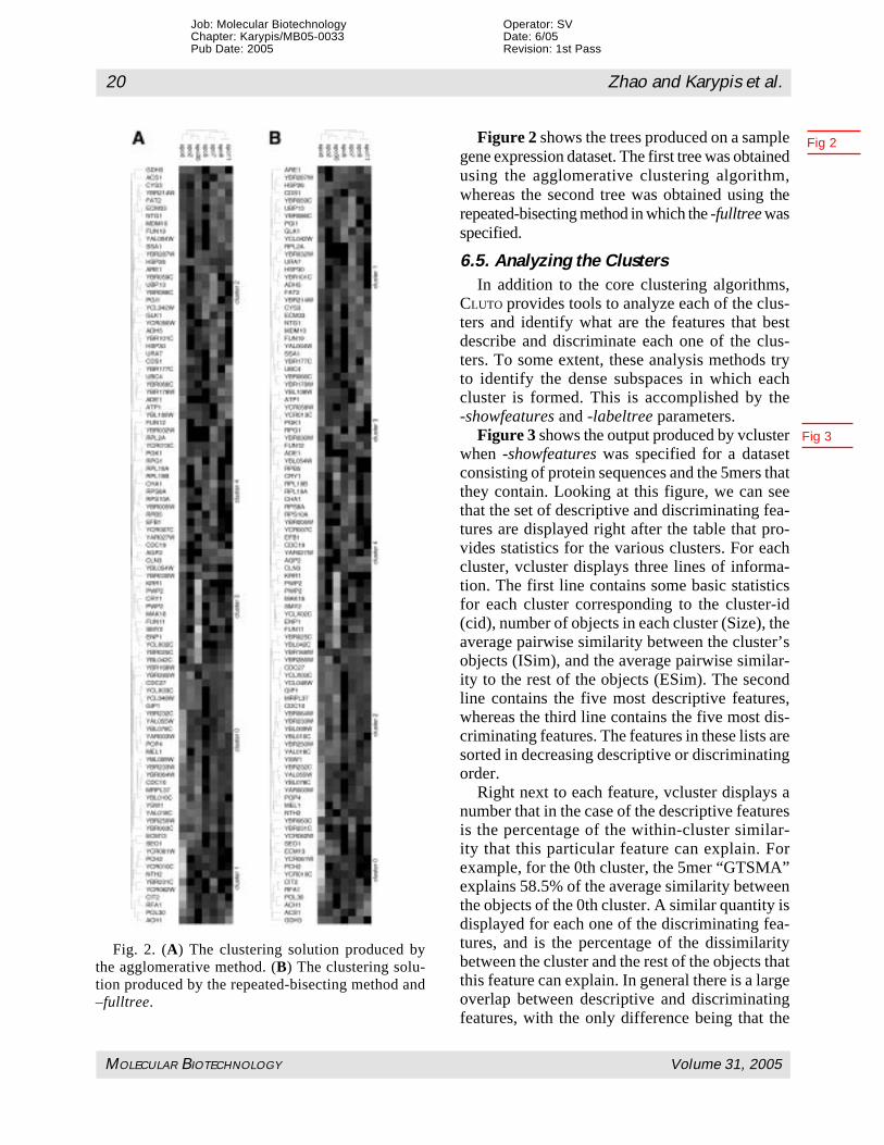
Figure 2 shows the trees produced on a samplegene expression dataset. The first tree was obtainedusing the agglomerative clustering algorithm,whereas the second tree was obtained using therepeated-bisecting method in which the -fulltree wasspecified.

6.5. Analyzing the ClustersIn addition to the core clustering algorithms,

CLUTO provides tools to analyze each of the clus-ters and identify what are the features that bestdescribe and discriminate each one of the clus-ters. To some extent, these analysis methods tryto identify the dense subspaces in which eachcluster is formed. This is accomplished by the-showfeatures and -labeltree parameters.

Figure 3 shows the output produced by vclusterwhen -showfeatures was specified for a datasetconsisting of protein sequences and the 5mers thatthey contain. Looking at this figure, we can seethat the set of descriptive and discriminating fea-tures are displayed right after the table that pro-vides statistics for the various clusters. For eachcluster, vcluster displays three lines of informa-tion. The first line contains some basic statisticsfor each cluster corresponding to the cluster-id(cid), number of objects in each cluster (Size), theaverage pairwise similarity between the cluster’sobjects (ISim), and the average pairwise similar-ity to the rest of the objects (ESim). The secondline contains the five most descriptive features,whereas the third line contains the five most dis-criminating features. The features in these lists aresorted in decreasing descriptive or discriminatingorder.

Right next to each feature, vcluster displays anumber that in the case of the descriptive featuresis the percentage of the within-cluster similar-ity that this particular feature can explain. Forexample, for the 0th cluster, the 5mer “GTSMA”explains 58.5% of the average similarity betweenthe objects of the 0th cluster. A similar quantity isdisplayed for each one of the discriminating fea-tures, and is the percentage of the dissimilaritybetween the cluster and the rest of the objects thatthis feature can explain. In general there is a largeoverlap between descriptive and discriminatingfeatures, with the only difference being that the

Fig 3

Fig. 2. (A) The clustering solution produced bythe agglomerative method. (B) The clustering solu-tion produced by the repeated-bisecting method and–fulltree.

Fig 2

Data Clustering 21



Fig. 3. Output of vcluster for matrix sports.mat and a 10-way clustering that shows the descriptive and dis-criminating features of each cluster.




Fig. 4. Various visualizations generated by the-plotmatrix (a) and -plotcluster (b) parameter.

Data Clustering 23



percentages associated with the discriminatingfeatures are typically smaller than the correspond-ing percentages of the descriptive features. Thisis because some of the descriptive features of acluster may also be present in a small fraction ofthe objects that do not belong to the cluster.

6.6. Visualizing the ClustersCLUTO’s programs can produce a number of

visualizations that can be used to see the rela-tionships between the clusters, objects, and fea-tures. You have already seen one of them in Fig. 2that was produced by the -plotmatrix parameter.The same parameter can be used to visualizesparse high-dimensional datasets. This is illus-trated in Fig. 4A for the protein dataset used ear-lier. As we can see from that plot, vcluster showsthe rows of the input matrix reordered in such away so that the rows assigned to each one of the10 clusters are numbered consecutively. The col-umns of the displayed matrix are selected to bethe union of the most descriptive and discriminat-ing features of each cluster, and are ordered accord-ing to the tree produced by an agglomerativeclustering of the columns. Also, at the top of eachcolumn, the label of each feature is shown. Eachnon-zero positive element of the matrix is dis-played by a different shade of red. Entries thatare bright red correspond to large values and thebrightness of the entries decreases as their valuedecrease. Also note that in this visualization boththe rows and columns have been reordered usinga hierarchical tree.

Finally, Fig. 4B shows the type of visualiza-tion that can be produced when -plotcluster isspecified for a sparse matrix. This plot shows theclustering solution shown at Fig. 4A by replacingthe set of rows in each cluster by a single row thatcorresponds to the centroid vector of the cluster.The -plotcluster option is particularly useful fordisplaying very large datasets, as the number of rowsin the plot is only equal to the number of clusters.

7. Future Research Directions in ClusteringDespite the huge body of research in cluster

analysis, there are a number of open problems andresearch opportunities, especially in the context

of clustering datasets arising in life sciences.Existing clustering algorithms for sequence andstructure datasets operate on the object’s similar-ity space. As discussed in Subheading 2.2., suchalgorithms are quite limiting as they cannot scaleto very large datasets, cannot be used to find clus-ters that have conserved features (e.g., sequenceor structural motifs), and cannot be used to pro-vide a description as to why a set of objects wasassigned to the same cluster that is native to theobject’s features. The only way to overcome theseshortcomings is to develop algorithms that oper-ate directly on either the sequences or structures.Thus, opportunities for future research can bebroadly categorized into three groups: (1) devel-opment of computationally efficient and scalablealgorithms for large sequence and structuredatasets; (2) development of clustering algo-rithms for sequence and structure datasets thatoperate directly on the object’s native representa-tion; and (3) development of clustering algo-rithms that can provide concise explanations onthe characteristics of the objects that were assignedto each cluster.

References1. Linial, M., Linial, N., Tishby, J., and Golan, Y.

(1997) Global self-organization of all known proteinsequences reveals inherent biological structures. J.Mol. Biol. 268, 539–556.

2. Enright, A. J. and Ouzounis, C. A. (2000) GeneRAGE:a robust algorithm for sequence clustering and domaindetection. Bioinformatics 16(5), 451–457.

3. Mian, I. S. and Dubchak, I. (2000) Representing and rea-soning about protein families using generative and dis-criminative methods. J. Comput. Biol. 7(6), 849–862.

4. Spang, R. and Vingron, M. (2001) Limits of homol-ogy of detection by pairwise sequence comparison.Bioinformatics 17(4), 338–342.

5. Kriventseva, E., Biswas, M., and Apweiler, R. (2001)Clustering and analysis of protein families. Curr.Opin. Struct. Biol. 11, 334–339.

6. Eidhammer, I., Jonassen, I., and Taylor, W. R. (2000)Structure comparison and stucture patterns. J. Comput.Biol. 7, 685–716.

7. Shatsky, M., Fligelman, Z. Y., Nussinov, R., andWolfson, H. J. (2000) Alignment of flexible proteinstructures, in Proceedings of the 8th InternationalConference on Intelligent Systems for Molecular Biol-ogy, (Altman, R., et al., eds.), AAAI Press, Menlo Park,CA, pp. 329–343.

Fig 4




8. Lee, R. C. T. (1981) Clustering analysis and its appli-cations, in Advances in Information Systems Science(Toum, J. T., ed.), Plenum, New York.

9. Jain, A. K. and Dubes, R. C. (1988) Algorithms forClustering Data, Prentice Hall, 1998.

10. Cheeseman, P. and Stutz, J. (1996) Bayesian classifi-cation (autoclass): theory and results, in Advances inKnowledge Discovery and Data Mining (Fayyad, U.M., Piatetsky-Shapiro, G., Smith, P., and Uthurusamy,R., eds.), AAAI/MIT Press, pp. 153–180.

11. Kaufman, L. and Rousseeuw, P. J. (1990) FindingGroups in Data: An Introduction to Cluster Analysis,John Wiley & Sons, New York.

12. Jackson, J. E. (1991) A User’s Guide to PrincipalComponents, John Wiley & Sons, New York.

13. Ng, R. and Han, J. (1994) Efficient and effective clus-tering method for spatial data mining, in Proceedingsof the 20th VLDB Conference (Bocca, J. B., Jarke,M., and Zaniolo, C., eds.), San Francisco, CA, pp.144–155.

14. Berry, M. W., Dumais, S. T., and O’Brien, G. W.(1995) Using linear algebra for intelligent informa-tion retrieval. SIAM Rev. 37, 573–595.

15. Zhang, T., Ramakrishnan, R., and Linvy, M. (1996)Birch: an efficient data clustering method for largedatabases, in Proceedings of 1996 ACM-SIGMODInternational Conference on Management of Data,ACM Press, New York, NY, pp. 103–114.

16. Ester, M., Kriegel, H.-P., Sander, J., and Xu, X.(1996) A density-based algorithm for discoveringclusters in large spatial databases with noise, in Pro-ceedings of the Second International Conference onKnowledge Discovery and Data Mining (Simoudis,E., Han, J., and Fayyad, U., eds.), AAAI Press, MenloPark, CA, pp. 226–231.

17. Wang, X., Wang, J. T. L., Shasha, D., Shapiro, B.,Dikshitulu, S., Rigoutsos, I., and Zhang, K. (1997)Automated discovery of active motifs in three dimen-sional molecules, in Proceedings of the 3rd Interna-tional Conference on Knowledge Discovery and DataMining (Heckerman, D., Mannila, H., Pregibon, D.,and Uthurusamy, R., eds.), AAAI Press, Menlo Park,CA, pp. 89–95.

18. Guha, S., Rastogi, R., and Shim, K. (1998) CURE: anefficient clustering algorithm for large databases, inProceedings of 1998 ACM-SIGMOD InternationalConference on Management of Data, ACM Press,New York, NY, pp. 73–84.

19. Guha, S., Rastogi, R., and Shim, K. (1999) ROCK: arobust clustering algorithm for categorical attributes,in Proceedings of the 15th International Conferenceon Data Engineering, IEEE, Washington-Brussels-Tokyo, pp. 512–521.

20. Karypis, G., Han, E. H., and Kumar, V. (1999) Cha-meleon: a hierarchical clustering algorithm usingdynamic modeling. IEEE Comput. 32(8), 68–75.

21. Jain, A. K., Murty, M. N., and Flynn, P. J. (1999)Data clustering: a review. ACM Comput. Surv. 31(3),264–323.

22. Han, J., Kamber, M., and Tung, A. K. H. (2001) Spa-tial clustering methods in data mining: a survey, inGeographic Data Mining and Knowledge Discovery(Miller, H. and Han, J., eds.), Taylor & Francis.

23. MacQueen, J. (1967) Some methods for classifica-tion and analysis of multivariate observations, in Pro-ceedings of the 5th Symposium Math. Statist. Prob.,pp. 281–297.

24. Dempster, A. P., Laird, N. M., and Rubin, D. B.(1977) Maximum likelihood from incomplete data viathe em algorithm. J. Roy. Stat. Soc. 39.

25. Zahn, K. (1971) Graph-theoretical methods for de-tecting and describing gestalt clusters. IEEE Trans.Comput. (C-20), 68–86.

26. Han, E. G., Karypis, G., Kumar, V., and Mobasher,B. (1998) Hypergraph based clustering in high-di-mensional data sets: a summary of results. Bull. Tech.Committee Data Eng. 21(1).

27. Strehl, A. and Ghosh, J. (2000) Scalable approach tobalanced, high-dimensional clustering of market-bas-kets, in Proceedings of HiPC, Springer Verlag, pp.525–536.

28. Boley, D. (1998) Principal direction divisive parti-tioning. Data Mining Knowl. Discov. 2(4),

29. Duda, R. O., Hart, P. E., and Stork, D. G. (2001) Pat-tern Classification, John Wiley & Sons, New York.

30. Zhao, Y. and Karypis, G. (2001) Criterion functionsfor document clustering: experiments and analysis.Technical report TR #01–40, Department of ComputerScience, University of Minnesota, Minneapolis. Avail-able at http://cs.umn.edu/ ~karypis/publications.

31. Sneath, P. H. and Sokal, R. R. (1973) Numerical Tax-onomy, Freeman, London, UK.

32. King, B. (1967) Step-wise clustering procedures. J. Am.Stat. Assoc. 69, 86–101.

33. Johnson, M. S., Sutcliffe, M. J., and Blundell, T. L.(1990) Molecular anatomy: phyletic relationshipsderived from 3-dimensional structures of proteins.J. Mol. Evol. 30, 43–59.

34. Taylor, W. R., Flores, T. P., and Orengo, C. A. (1994)Multiple protein structure alignment. Protein Sci. 3,1858–1870.

35. Jonyer, I., Holder, L. B., and Cook, D. J. (2000)Graph-based hierarchical conceptual clustering instructural databases. Int. J. Artific. Intell. Tools.

36. Eddy, S. R. (1996) Hidden markov models. Curr.Opin. Struct. Biol. 6, 361–365.

37. Eddy, S. R. (1998) Profile hidden markov models.Bioinformatics 14, 755–763.

38. Aggarwal, C. C., Gates, S. C., and Yu, P. S. (1999)On the merits of building categorization systems bysupervised clustering, Proceedings of the Fifth ACMSIGKDD International Conference on KnowledgeDiscovery and Data Mining (Chaudhuri, S. and

Data Clustering 25



Madigan, D., eds.), ACM Press, New York, NY, pp.352–356.

39. Cutting, D. R., Pedersen, J. O., Karger, D. R., andTukey, J. W. (1992) Scatter/gather: a cluster-basedapproach to browsing large document collections, inProceedings of the ACM SIGIR, ACM Press, NewYork, NY, pp. 318–329.

40. Larsen, B. and Aone, C. (1999) Fast and effective textmining using linear-time document clustering, inProceedings of the Fifth ACM SIGKDD InternationalConference on Knowledge Discovery and Data Min-ing (Chaudhuri, S. and Madigan, D., eds.), ACMPress, New York, NY, pp. 16–22.

41. Steinbach, M., Karypis, G., and Kumar, V. (2000) Acomparison of document clustering techniques, inKDD Workshop on Text Mining, ACM Press, NewYork, NY, pp. 109–110.

42. Agrawal, R., Gehrke, J., Gunopulos, D., and Raghavan,P. (1998) Automatic subspace clustering of high di-mensional data for data mining applications, in Proceed-ings of 1998 ACM-SIGMOD International Conferenceon Management of Data, ACM Press, New York, NY,pp. 94–105.

43. Burdick, D., Calimlim, M., and Gehrke, J. (2001)Mafia: a maximal frequent itemset algorithm fortransactional databases, in Proceedings of the 17thInternational Conference on Data Engineering,IEEE, Washington-Brussels-Tokyo, pp. 443–452.

44. Nagesh, H., Goil, S., and Choudhary, A. (1999) Ma-fia: efficient and scalable subspace clustering for verylarge data sets. Technical report TR #9906-010,Northwestern University.

45. Huang, Z. (1997) A fast clustering algorithm to clus-ter very large categorical data sets in data mining, inProceedings of SIGMOD Workshop on ResearchIssues on Data Mining and Knowledge Discovery,Tucson, Arizona.

46. Ganti, V., Gehrke, J., and Ramakrishnan, R., (1999)Cactus-clustering categorical data using summaries, inProceedings of the 5th International Conference onKnowledge Discovery and Data Mining (Chaudhuri,S. and Madigan, D., eds.), ACM Press, New York, NY,pp. 73–83.

47. Gibson, D., Kleinberg, J., and Rahavan, P. (1998) Clus-tering categorical data: an approach based on dynamicalsystems, in Proceedings of the 24th International Con-ference on Very Large Databases (Gupta, A., Shmueli,O., and Widom, J., eds.), pp. 311–323, San Francisco,CA, Morgan Kaufmann.

48. Ryu, T. W. and Eick, C. F. (1998) A unified similar-ity measure for attributes with set or bag of values fordatabase clustering, in The 6th International Work-shop on Rough Sets, Data Mining and Granular Com-puting, Research Triangle Park, NC.

49. Gusfield, D. (1997) Algorithms on Strings, Trees, andSequences: Computer Science and ComputationalBiology, Cambridge University Press, NY.

50. Dayhoff, M. O., Schwartz, R. M., and Orcutt, B. C.(1978) A model of evolutionary change in proteins.Atlas Protein Sequence Struct. 5, 345–352.

51. Schwartz, R. M. and Dayhoff, M. O. (1978) Matricesfor detecting distant relationships. Atlas Protein Se-quence Struct. 5, 353–358.

52. Henikoff, S. and Henikoff, J. G. (1992) Amino acidsubstitution matrices from protein blocks. Proc. Natl.Acad. Sci. USA 89, 10,915–10,919.

53. Needleman, S. B. and Wunsch, C. D. (1970) A gen-eral method applicable to the search for similaritiesin the amino acid sequence of two proteins. J. Mol.Biol. 48, 443–453.

54. Smith, T. F. and Waterman, M. S. (1981) Identifica-tion of common molecular subsequences. J. Mol.Biol. 147, 195–197.

55. Lipman, D. J. and Pearson, W. R. (1985) Rapid andsensitive protein similarity searches. Science 227,1435–1441.

56. Pearson, W. R. and Lipman, D. J. (1988) Improvedtools for biological sequence comparison. Proc. Natl.Acad. Sci. USA 85, 2444–2448.

57. Altschul, S., Gish, W., Miller, W., Myers, E., andLipman, D. (1990) Basic local alignment search tool.J. Mol. Biol. 215, 403–410.

58. Yona, G., Linial, N., and Linial, M. (2000) Protomap:automatic classification of protein sequences and hier-archy of protein families. Nucleic Acids Res. 28, 49–55.

59. Bolten, E., Schliep, A., Schneckener, S., Schomburg,D., and Schrader, R. (2001) Clustering protein se-quences-structure prediction by transitive homology.Bioinformatics 17, 935–941.

60. Johnson, M. S. and Lehtonen, J. V. (2000) Compari-son of protein three dimensional structure, in Bio-informatics: Sequences, Structure and Databanks(Higgins, D, eds.), Oxford University Press, 2000.

61. Grindley, H. M., Artymiuk, P. J., Rice, D. W., andWillet, P. (1993) Identification of tertiary structureresemblance in proteins using a maximal commonsubgraph isomorphism algorithm. J. Mol. Biol. 229,707–721.

62. Mitchell, E. M., Artymiuk, P. J., Rice, D. W., andWillet, P. (1989) Use of techniques derived fromgraph theory to compare secondary structure motifsin proteins. J. Mol. Biol. 212, 151–166.

63. Holm, L. and Sander, C. (1993) Protein structurecomparison by alignment of distance matrices. J.Mol. Biol. 233, 123.

64. Kleywegt, G. J. and Jones, T. A. (1997) Detectingfolding motifs and similarities in protein structures.Methods Enzymol. 277, 525–545.

65. Calinski, T. and Harabasz, J. (1974) A dendritemethod for cluster analysis. Commun. Stat. 3, 1–27.

66. Ben-Hur, A., Elisseeff, A., and Guyon, I. (2000) A sta-bility based method for discovering structure in clus-tered data, in Pacific Symposium on Biocomputing, vol.7, World Scientific Press, Singapore, pp. 6–17.




67. Yeung, K. Y., Haynor, D. R., and Ruzzo, W. L.(2001) Validating clustering for gene expression data.Bioinformatics 17(4), 309–318.

68. Fodor, S. P., Rava, R. P., Huang, X. C., Pease, A. C.,Holmes, C. P., and Adams, C. L. (1993) Multiplexedbiochemical assays with biological chips. Nature 364,555, 556.

69. Schena, M., Shalon, D., Davis, R. W., and Brown, P.O. (1995) Quantitative monitoring of gene expressionpatterns with a complementary DNA microarray. Sci-ence 270.

70. Brazma, A., Robinson, A., Cameron, G., and Ashburner,M. (2000) One-stop shop for microarray data. Nature403, 699–701.

71. Yang, Y. H., Dudoit, S., Luu, P., and Speed, T. P.(2001) Normalization for cDNA microarray data, inProceedings of SPIE International Biomedical Op-tics Symposium (Bittner, M. L., Chen, Y., Dorsel, A.N., and Dougherty, E. R., eds.), vol. 4266, SPIE,Bellingham, WA, pp. 141–152.

72. D’Haeseleer, P., Fuhrman, S., Wen, X., and Somogyi,R. (1998) Mining the gene expression matrix: infer-ring gene relationships from large scale gene expres-sion data, in, Information Processing in Cells andTissues, Plenum, New York, pp. 203–212.

73. Eisen, M. (2000) Cluster 2.11 and treeview 1.50 http://rana.lbl.gov/Eisen Software.htm.

74. Tamayo, P., Slonim, D., Mesirov, J., Zhu, Q.,Kitareewan, S., Dmitrovsky, E., Lander, E. S., andGolub, T. R. (1999) Interpreting patterns of geneexpression with self-organizing maps: methods and

application to hematopoietic differentiation. Proc.Natl. Acad. Sci. USA 96, 2907–2912.

75. Kohonen, T. Self-Organizing Maps, Springer-Verlag,Berlin, 1995.

76. Ben-Dor, A. and Yakhini, Z. (1999) Clustering geneexpression patterns, in Proceedings of the 3rd AnnualInternational Conference on Research in Computa-tional Molecular Biology, ACM Press, New York,NY, pp. 33–42.

77. Shamir, R. and Sharan, R. (2000) Click: a clusteringalgorithm for gene expression analysis, in Proceed-ings of the 8th International Conference on Intelli-gent Systems for Molecular Biology (Altman, R., etal., eds.), AAAI Press, Menlo Park, CA, pp. 307–316.

78. Zhao, Y. and Karypis, G. (2002) Comparison ofagglomerative and partitional document clusteringalgorithms, in SIAM (2002) Workshop on ClusteringHigh-Dimensional Data and Its Applications. Arling-ton, VA. Also available as technical report #02-014,University of Minnesota.

79. Karypis, G. and Kumar, V. (1998) hMeTiS 1.5: ahypergraph partitioning package. Technical report,Department of Computer Science, University ofMinnesota. Available at www-users.cs.umn.edu/~karypis/metis

80. Karypis, G. and Kumar, V. (1998) MeTiS 4.0: unstruc-tured graph partitioning and sparse matrix orderingsystem. Technical report, department of Computer Sci-ence, University of Minnesota. Available at www-users.cs.umn.edu/~karypis/metis

data clustering in life sciences - glaros.dtc.umn.edu

Documents