data base management system paper code: bca 110 paper …

DATA BASE MANAGEMENT SYSTEM

Paper Code: BCA 110

Paper ID: 20110 3 1 4

UNIT-I

Introduction: An overview of database management system, database system Vs files system,

Characteristics of database approach, DBMS architecture, data models, schema and instances,

data independence.

Data Modeling using Entity Relationship Model: Entity, Entity types, entity set, notation for

ER diagram, attributes and keys, Concepts of composite, derived and multivalve attributes,

Super Key, candidate key, primary key, relationships, relation types, weak entities, enhanced

E-R and object modeling, Sub Classes:, Super classes, inheritance, specialization and

generalization.[T1],T2][T3][R1]

UNIT – II

Introduction to SQL: Overview, Characteristics of SQL. Advantage of SQL, SQL data types

And literals.

Types of SQL commands: DDL, DML, DCL. Basic SQL Queries.

Logical operators: BETWEEN, IN, AND, OR and NOT

Null Values: Disallowing Null Values, Comparisons Using Null Values

Integrity constraints: Primary Key, Not NULL, Unique, Check, Referential key

Introduction to Nested Queries, Correlated Nested Queries, Set-Comparison Operators,

Aggregate Operators: The GROUP BY and HAVING Clauses,

Joins: Inner joins, Outer Joins, Left outer, Right outer, full outer joins.

Overview of views and indexes. [T1],[R2] [No. of Hrs.: 12]

Note : A Minimum of 40 Lectures is mandatory for each course.

Syllabus of Bachelor of Computer Applications (BCA), approved by BCA Coordination

Committee on 26th July 2011 & Sub-

Committee Academic Council held 28th July 2011. W.e.f. academic session 2011-12

UNIT – III

Relational Data Model: Relational model terminology domains, Attributes, Tuples, Relations,

Characteristics of relations, relational constraints domain constraints, key constraints and

constraints on null, relational DB schema.Codd’s Rules

Relational algebra: Basic operations selection and projection,

Set Theoretic operations Union, Intersection, set difference and division,

Join operations: Inner , Outer ,Left outer, Right outer and full outer join.

ER to relational Mapping: Data base design using ER to relational language.

Data Normalization: Functional dependencies, Armstrong’s inference rule, Normal form up to

3rd normal form. [T1],T2][T3][R1] [No. of Hrs.: 12]

UNIT – IV

Transaction processing and Concurrency Control: Definition of Transaction, Desirable

ACID properties, overview of serializability, serializable and non serializable transactions

Concurrency Control: Definition of concurrency, lost update, dirty read and incorrect

Summary problems due to concurrency

Concurrency Control Techniques: Overview of Locking, 2PL, Timstamp ordering,

Multi versioning, validation

Elementary concepts of Database security: system failure, Backup and Recovery Techniques,

Authorization and authentication.

UNIT 1

INTRODUCTION: An overview of database management system:- database is an organized

collection of data. The data is typically organized to model relevant aspects of reality (for

example, the availability of rooms in hotels), in a way that supports processes requiring this

information (for example, finding a hotel with vacancies).

Database management systems (DBMSs) are specially designed applications that interact with

the user, other applications, and the database itself to capture and analyze data. A general-

purpose database management system (DBMS) is a software system designed to allow the

definition, creation, querying, update, and administration of databases. Well-known DBMSs

include MYSQL, SQLITE, MICROSOFT SQL SERVER, ORACLE, SAP DBASE, FOXPRO,

IBMDB2. A database is not generally PORTABLE across different DBMS, but different DBMSs

can INTER OPERATE by using STANDARDS such as SQL and ODBC or JDBC to allow a

single application to work with more than one database.

Formally, the term "database" refers to the data itself and supporting data structure Databases are

created to operate large quantities of information by inputting, storing, retrieving, and managing

that information. Databases are set up, so that one set of software programs provides all users

with access to all the data. Databases use a table format that is made up of rows and columns.

Each piece of information is entered into a row, which then creates a record. Once the records

are created in the database, they can be organized and operated in a variety of ways that are

limited mainly by the software being used. Databases are somewhat similar to spreadsheets, but

databases are more demanding than spreadsheets because of their ability to manipulate the data

that is stored. It is possible to do a number of functions with a database that would be more

difficult to do with a spreadsheet. The word data is normally defined as facts from which

information can be derived. A database may contain millions of such facts. From these facts the

database management system (DBMS) can develop information.

A "database management system" (DBMS) is a suite of computer software providing the

interface between users and a database or databases. Because they are so closely related, the term

"database" when used casually often refers to both a DBMS and the data it manipulates.

Outside the world of professional information technology, the term database is sometimes used

casually to refer to any collection of data (perhaps a spreadsheet, maybe even a card index). This

article is concerned only with databases where the size and usage requirements necessitate use of

a database management system. The interactions catered for by most existing DBMS fall into

four main groups:

Data definition. Defining new data structures for a database, removing data structures from the

database, modifying the structure of existing data.

Update. Inserting, modifying, and deleting data.

Retrieval. Obtaining information either for end-user queries and reports or for processing by

applications.

Administration. Registering and monitoring users, enforcing data security, monitoring

performance, maintaining data integrity, dealing with concurrency control, and recovering

information if the system fails.

A DBMS is responsible for maintaining the integrity and security of stored data, and for

recovering information if the system fails.

Both a database and its DBMS conform to the principles of a particular data base model

"Database system" refers collectively to the database model, database management system, and

database

Database Management System Vs File Management System:

A Database Management System (DMS) is a combination of computer software, hardware, and

information designed to electronically manipulate data via computer processing. Two types of

database management systems are DBMS’s and FMS’s. In simple terms, a File Management

System (FMS) is a Database Management System that allows access to single files or tables at a

time. FMS’s accommodate flat files that have no relation to other files. The FMS was the

predecessor for the Database Management System (DBMS), which allows access to multiple

files or tables at a time (see Figure 1 below)

File Management Systems

Advantages Disadvantages

Simpler to use Typically does not support multi-user access

Less expensive· Limited to smaller databases

Fits the needs of many small businesses and

home users

Limited functionality (i.e. no support for

complicated transactions, recovery, etc.)

Popular FMS’s are packaged along with the

operating systems of personal computers (i.e.

Microsoft Cardfile and Microsoft Works)

Decentralization of data

Good for database solutions for hand held

devices such as Palm Pilot Redundancy and Integrity issues

Typically, File Management Systems provide the following advantages and disadvantages:

The goals of a File Management System can be summarized as follows (Calleri, 2001):

Management. An FMS should provide data management services to the application.

Generality with respect to storage devices. The FMS data abstractions and access methods

should remain unchanged irrespective of the devices involved in data storage.

Validity. An FMS should guarantee that at any given moment the stored data reflect the

operations performed on them.

Protection. Illegal or potentially dangerous operations on the data should be controlled by the

FMS.

Concurrency. In multiprogramming systems, concurrent access to the data should be allowed

with minimal differences.

Performance. Compromise data access speed and data transfer rate with functionality.

From the point of view of an end user (or application) an FMS typically provides the following

functionalities (Calleri, 2001):

File creation, modification and deletion.

Ownership of files and access control on the basis of ownership permissions.

Facilities to structure data within files (predefined record formats, etc).

Facilities for maintaining data redundancies against technical failure (back-ups, disk mirroring,

etc.).

Logical identification and structuring of the data, via file names and hierarchical directory

structures.

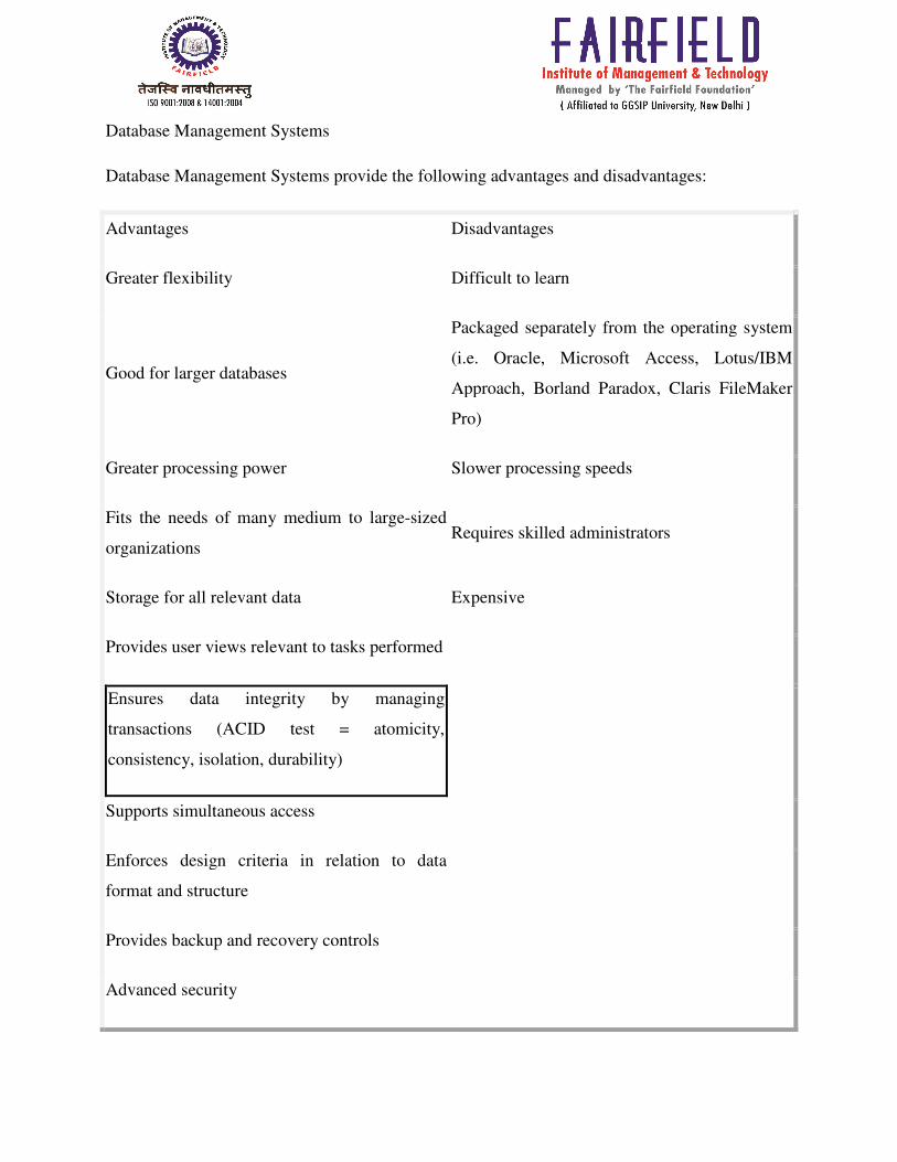
Database Management Systems

Database Management Systems provide the following advantages and disadvantages:

Advantages Disadvantages

Greater flexibility Difficult to learn

Good for larger databases

Packaged separately from the operating system

(i.e. Oracle, Microsoft Access, Lotus/IBM

Approach, Borland Paradox, Claris FileMaker

Pro)

Greater processing power Slower processing speeds

Fits the needs of many medium to large-sized

organizations Requires skilled administrators

Storage for all relevant data Expensive

Provides user views relevant to tasks performed

Ensures data integrity by managing

transactions (ACID test = atomicity,

consistency, isolation, durability)

Supports simultaneous access

Enforces design criteria in relation to data

format and structure

Provides backup and recovery controls

Advanced security

The goals of a Database Management System can be summarized as follows (Connelly, Begg,

and Strachan, 1999, pps. 54 – 60):

Data storage, retrieval, and update (while hiding the internal physical implementation

details)

A user-accessible catalog

Transaction support

Concurrency control services (multi-user update functionality)

Recovery services (damaged database must be returned to a consistent state)

Authorization services (security)

Support for data communication Integrity services (i.e. constraints)

Services to promote data independence

Utility services (i.e. importing, monitoring, performance, record deletion, etc.)

The components to facilitate the goals of a DBMS may include the following:

Query processor

Data Manipulation Language preprocessor

Database manager (software components to include authorization control, command processor,

integrity checker, query optimizer, transaction manager, scheduler, recovery manager, and buffer

manager)

Data Definition Language compiler

File manager

Characteristics of the Database Approach

Self-Describing Nature of Database System Insulation between Programs and Data, and Dataν

Abstraction Support of Multiple Views of the Data Sharing of Data and Multiuser Transaction

Processing. Self-Describing Nature of a Database System

A complete definition or description of theν database structure and constraints

DBMS software works equally well with anyν number of database applications

DBMS catalog stores the description of theν database. The description is called meta-data

Insulation between Programs and Data, and Data Abstraction Program-data independence

Allows changing data storage structures and operations without having to change the DBMS

access

Program - operation independence :-

The interface (or signature) of an operation includes the operation name and the data types of its

arguments (or parameters).The implementation (or method) of the operation is specified

separately and can be changed without affecting the interface.

Data Abstraction:

A data model is used to hide storage details and present the users with a conceptual view of the

database Support of Multiple Views of the Data.

A database typically has many users, each ofν whom may require a different perspective or view

of the database. A view may be a subset of the database or it may contain virtual data that is

derived from the database files but is not explicitly stored multiuser DBMS whose usersν have a

variety of applications must provide facilities for defining multiple views. Sharing of Data and

Multiuser Transaction Processing Allow multiple users to access the database at the same time.

Concurrency control allowing a set of concurrent users to retrieveν and to update the database.

Concurrency control within the DBMS guaranteesν that each transaction is correctly executed or

completely aborted.OLTP (Online Transaction Processing) is a major part of database

applications.

DBMS architecture:-

EXTERNAL LEVEL:

How data is viewed by an individual user

CONCEPTUAL LEVEL:

How data is viewed by a community of users

INTERNAL LEVEL:

How data is physically stored in the data base.

DATA MODELS:

DATA MODELS: A data model is a collection of concepts that can be used to describe the

structure of a database.

Data models can be broadly distinguished into 3 main categories-

1) high-level or conceptual data models (based on entities & relationships)

It provides concepts that are close to the way many users perceive data.

2) Low-level or physical data models

It provides concepts that describe the details of how data is stored in the computer.

These concepts are meant for computer specialist, not for typical end users.

3) Representational or implementation data models (record-based, object-oriented)

It provides concepts that can be understood by end users. These hide some details of data storage

but can be implemented on a computer system directly.

Hierarchical Model:

The hierarchical data model organizes data in a tree structure. There is a hierarchy of parent and

child data segments. This structure implies that a record can have repeating information,

generally in the child data segments. Data in a series of records, which have a set of field values

attached to it. It collects all the instances of a specific record together as a record type. These

record types are the equivalent of tables in the relational model, and with the individual records

being the equivalent of rows. To create links between these record types, the hierarchical model

uses Parent Child Relationships. These are a 1: N mapping between record types. This is done by

using trees, like set theory used in the relational model, "borrowed" from maths. For example, an

organization might store information about an employee, such as name, employee number,

department, salary. The organization might also store information about an employee's children,

such as name and date of birth. The employee and children data forms a hierarchy, where the

employee data represents the parent segment and the children data represents the child segment.

Network Model:

The popularity of the network data model coincided with the popularity of the hierarchical data

model. Some data were more naturally modeled with more than one parent per child. So, the

network model permitted the modeling of many-to-many relationships in data. In 1971, the

Conference on Data Systems Languages (CODASYL) formally defined the network model. The

basic data modeling construct in the network model is the set construct. A set consists of an

owner record type, a set name, and a member record type. A member record type can have that

role in more than one set; hence the multiparent concept is supported. An owner record type can

also be a member or owner in another set. The data model is a simple network, and link and

intersection record types (called junction records by IDMS) may exist, as well as sets between

them . Thus, the complete network of relationships is represented by several pair wise sets; in

each set some (one) record type is owner (at the tail of the network arrow) and one or more

record types are members (at the head of the relationship arrow). Usually, a set defines a 1: M

relationship, although 1:1 is permitted. The CODASYL network model is based on mathematical

set theory.

Relational Model:

(RDBMS - relational database management system) A database based on the relational model

developed by E.F. Codd. A relational database allows the definition of data structures, storage

and retrieval operations and integrity constraints. In such a database the data and relations

between them are organized in tables. A table is a collection of records and each record in a table

contains the same fields. This can be extended to joining multiple tables on multiple fields.

Because these relationships are only specified at retrieval time, relational databases are classed as

dynamic database management system. The RELATIONAL database model is based on the

Relational Algebra

Properties of Relational Tables:

1. Values Are Atomic

2. Each Row is Unique

3. Column Values Are of the Same Kind

4. The Sequence of Columns is Insignificant

5. The Sequence of Rows is Insignificant

6. Each Column Has a Unique Name

Certain fields may be designated as keys, which means that searches for specific values of that

field will use indexing to speed them up. Where fields in two different tables take values from

the same set, a join operation can be performed to select related records in the two tables by

matching values in those fields.

Object/Relational Model:

Object/relational database management systems (ORDBMSs) add new object storage capabilities

to the relational systems at the core of modern information systems. These new facilities

integrate management of traditional fielded data, complex objects such as time-series and

geospatial data and diverse binary media such as audio, video, images, and applets. By

encapsulating methods with data structures, an ORDBMS server can execute complex analytical

and data manipulation operations to search and transform multimedia and other complex objects.

Object-Oriented Model:

Object DBMSs add database functionality to object programming languages. They bring much

more than persistent storage of programming language objects. Object DBMSs extend the

semantics of the C++, Smalltalk and Java object programming languages to provide full-featured

database programming capability, while retaining native language compatibility. A major benefit

of this approach is the unification of the application and database development into a seamless

data model and language environment. As a result, applications require less code, use more

natural data modeling, and code bases are easier to maintain. Object developers can write

complete database applications with a modest amount of additional effort.

According to Rao (1994), "The object-oriented database (OODB) paradigm is the combination of

object-oriented programming language (OOPL) systems and persistent systems. The power of

the OODB comes from the seamless treatment of both persistent data, as found in databases, and

transient data, as found in executing programs.

Schema And Instances: - In DBMS,Schema is the overall Design of the Database. Instance is

the information stored in the Database at a particular moment. In programming, you declare a

variable which Physical Schema describes database design at physical level while a logical

schema describes the database design at the logical level. A database may also have several

schemas at the view level, sometimes called subschema’s, that describe different views of the

database corresponds to "Schema”. But its values changes as and when required which

corresponds to "Instance”.

The data in the database at a particular moment of time is called an instance or a database state.

In a given instance, each schema construct has its own current set of instances. Many instances

or database states can be constructed to correspond to a particular database schema. Every time

we update (i.e., insert, delete or modify) the value of a data item in a record, one state of the

database changes into another state.

A schema is plan of the database that give the names of the entities and attributes and the

relationship among them. A schema includes the definition of the database name, the record type

and the components that make up the records. Alternatively, it is defined as a framework into

which the values of the data items are fitted. The values fitted into the frame-work changes

regularly but the format of schema remains the same e.g., consider the database consisting of

three files ITEM, CUSTOMER and SALES.

Generally, a schema can be partitioned into two categories, i.e., (i) Logical schema and (ii)

Physical schema.

i) The logical schema is concerned with exploiting the data structures offered by the DBMS so

that the schema becomes understandable to the computer. It is important as programs use it to

construct applications.

ii) The physical schema is concerned with the manner in which the conceptual database get

represented in the computer as a stored database. It is hidden behind the logical schema and can

usually be modified without affecting the application programs.

The DBMS's provide DDL and DSDL to specify both the logical and physical schema.

Subschema:

A subschema is a subset of the schema having the same properties that a schema has. It identifies

a subset of areas, sets, records, and data names defined in the database schema available to user

sessions. The subschema allows the user to view only that part of the database that is of interest

to him. The subschema defines the portion of the database as seen by the application programs

and the application programs can have different view of data stored in the database.

DATA INDEPENDENCE :-

A major objective for three-level architecture is to provide data independence, which means that

upper levels are unaffected by changes in lower levels.

There are two kinds of data independence:

• Logical data independence

• Physical data independence

Logical Data Independence:-Logical data independence indicates that the conceptual schema

can be changed without affecting the existing external schemas. The change would be absorbed

by the mapping between the external and conceptual levels. Logical data independence also

insulates application programs from operations such as combining two records into one or

splitting an existing record into two or more records. This would require a. change in the

external/conceptual mapping so as to leave the external view unchanged.

Physical Data Independence:-Physical data independence indicates that the physical storage

structures or devices could be changed without affecting conceptual schema. The change would

be absorbed by the mapping between the conceptual and internal levels. Physic 1data

independence is achieved by the presence of the internal level of the database and the n, lPping

or transformation from the conceptual level of the database to the internal level. Conceptual level

to internal level mapping, therefore provides a means to go from the conceptual view (conceptual

records) to the internal view and hence to the stored data in the database (physical records).

If there is a need to change the file organization or the type of physical device used as a result of

growth in the database or new technology, a change is required in the conceptual/ internal

mapping between the conceptual and internal levels. This change is necessary to maintain the

conceptual level invariant. The physical data independence criterion requires that the conceptual

level does not specify storage structures or the access methods (indexing, hashing etc.) used to

retrieve the data from the physical storage medium. Making the conceptual schema physically

data independent means that the external schema, which is defined on the conceptual schema, is

in turn physically data independent.

The Logical data independence is difficult to achieve than physical data independence as it

requires the flexibility in the design of database and prograll1iller has to foresee the future

requirements or modifications.

Data Modeling using Entity Relationship Model: An ER model is an abstract way of

describing a database. In the case of a relational database, which stores data in tables, some of

the data in these tables point to data in other tables - for instance, your entry in the database

could point to several entries for each of the phone numbers that are yours. The ER model would

say that you are an entity, and each phone number is an entity, and the relationship between you

and the phone numbers is 'has a phone number'. Diagrams created to design these entities and

relationships are called entity–relationship diagrams or ER diagrams.

Using the three schema approach to software engineering, there are three levels of ER models

that may be developed.

Conceptual data model:

This is the highest level ER model in that it contains the least granular detail but establishes the

overall scope of what is to be included within the model set. The conceptual ER model normally

defines master reference data entities that are commonly used by the organization. Developing an

enterprise-wide conceptual ER model is useful to support documenting the data architecture for

an organization.

A conceptual ER model may be used as the foundation for one or more logical data models (see

below). The purpose of the conceptual ER model is then to establish structural metadata

commonality for the master data entities between the set of logical ER models. The conceptual

data model may be used to form commonality relationships between ER models as a basis for

data model integration.

Logical data model:

A logical ER model does not require a conceptual ER model, especially if the scope of the

logical ER model is to develop a single disparate information system. The logical ER model

contains more detail than the conceptual ER model. In addition to master data entities,

operational and transactional data entities are now defined. The details of each data entity are

developed and the entity relationships between these data entities are established. The logical ER

model is however developed independent of technology into which it will be implemented.

Physical model

One or more physical ER models may be developed from each logical ER model. The physical

ER model is normally developed to be instantiated as a database. Therefore, each physical ER

model must contain enough detail to produce a database and each physical ER model is

technology dependent since each database management system is somewhat different.

The physical model is normally forward engineered to instantiate the structural metadata into a

database management system as relational database objects such as database tables, database

indexes such as unique key indexes, and database constraints such as a foreign key constraint or

a commonality constraint. The ER model is also normally used to design modifications to the

relational database objects and to maintain the structural metadata of the database.

Entity, Entity types, entity set :- An entity may be defined as a thing which is recognized as

being capable of an independent existence and which can be uniquely identified. An entity is an

abstraction from the complexities of a domain. When we speak of an entity, we normally speak

of some aspect of the real world which can be distinguished from other aspects of the real world

An entity may be a physical object such as a house or a car, an event such as a house sale or a car

service, or a concept such as a customer transaction or order. Although the term entity is the one

most commonly used, following Chen we should really distinguish between an entity and an

entity-type. An entity-type is a category. An entity, strictly speaking, is an instance of a given

entity-type. There are usually many instances of an entity-type. Because the term entity-type is

somewhat cumbersome, most people tend to use the term entity as a synonym for this term.

Entities can be thought of as nouns. Examples: a computer, an employee, a song, a mathematical

theorem. Entities and relationships can both have attributes. Examples: an employee entity might

have a Social Security Number (SSN) attribute; the proved relationship may have a date

attribute.

Every entity (unless it is a weak entity) must have a minimal set of uniquely identifying

attributes, which is called the entity's primary key .

Entity–relationship diagrams don't show single entities or single instances of relations. Rather,

they show entity sets and relationship sets. Example: a particular song is an entity. The collection

of all songs in a database is an entity set. The eaten relationship between a child and her lunch is

a single relationship. The set of all such child-lunch relationships in a database is a relationship

set. In other words, a relationship set corresponds to a relation in mathematics.

A set of entities that have the same attributes is called an entity type. Each entity type in the

database is described by a name and a list of attributes. For example an entity employee is an

entity type that has Name, Age and Salary attributes.

The individual entities of a particular entity type are grouped into a collection or entity set, which

is also called the extension of the entity type.

An entity is a thing in the real world. It may be an object with a physical existence or an object

with a conceptual existence. A set of these entities having same attributes is entity type and

collection of individual entity type is an entity set

Entity set: the collection of all entities of a particular entity type in the database at any point of

time is called Entity set. An entity set is a set of entities of the same type, Entity sets need not be

disjoint. For example, the entity set employee (all employees of a bank) and the entity set

customer (all customers of the bank) may have members in common. An entity set is a logical

container for instances of an entity type and instances of any type derived from that entity type.

(For information about derived types, see Entity data model inheritance) The relationship

between an entity type and an entity set is analogous to the relationship between a row and a

table in a relational database: Like a row, an entity type describes data structure, and, like a table,

an entity set contains instances of a given structure. An entity set is not a data modeling

construct; it does not describe the structure of data. Instead, an entity set provides a construct for

a hosting or storage environment (such as the common language runtime or a SQL Server

database) to group entity type instances so that they can be mapped to a data store.

An entity set is defined within an entity container, which is a logical grouping of entity sets and

association set.For an entity type instance to exist in an entity set, the following must be true:

The type of the instance is either the same as the entity type on which the entity set is based, or

the type of the instance is a subtype of the entity type.

The entity key for the instance is unique within the entity set.

The instance does not exist in any other entity set.

Notation for Er Diagram: - Start to Draw a Entity Relationship Diagram The steps involved in

creating an entity relationship diagram are:

1 .Identify the entities.

2. Determine all significant interactions.

3. Analyze the nature of the interactions.

4. Draw the entity relationship diagram.

When you create an entity relationship diagram one of the first things that you consider is the

entities about which you wish to record information. For example, in a family database you

probably wish to record information about member, house, job, love, contact, etc. However, in a

relational database you record not only details about the entities but also the relationship between

these entities. For example, in the family members are assigned to house and every member is

appointed to be in charge of each love and job. Entities are the "things" about which you wish to

record information in a database. There are relationships between entities which fall into three

types: one-one, one-many, many-many. Any many-many relationship must be resolved into two

one-many relationships.

Steps that is used in ER-diagram:- Identify all the relevant entities in a given system and

determine the relationships among these entities.

An entity should appear only once in a particular diagram.

Provide a precise and appropriate name for each entity, attribute, and relationship in the diagram.

Terms that are simple and familiar always beats vague, technical-sounding words. In naming

entities, remember to use singular nouns. However, adjectives may be used to distinguish entities

belonging to the same class (part-time employee and full time employee, for example).

Meanwhile attribute names must be meaningful, unique, system-independent, and easily

understandable.

Remove vague, redundant or unnecessary relationships between entities.

Never connect a relationship to another relationship.

Make effective use of colors. You can use colors to classify similar entities or to highlight key

areas in your diagrams

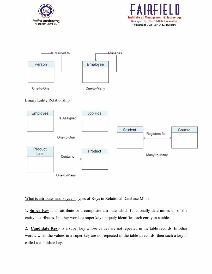
Binary Entity Relationship

What is attributes and keys :- Types of Keys in Relational Database Model

1. Super Key is an attribute or a composite attribute which functionally determines all of the

entity’s attributes. In other words, a super key uniquely identifies each entity in a table.

2. Candidate Key:- is a super key whose values are not repeated in the table records. In other

words, when the values in a super key are not repeated in the table’s records, then such a key is

called a candidate key.

3. Primary Key is a candidate key who doesn’t have repeated values nor does it comes with a

NULL value in the table. A primary key can uniquely identifies each row in any table, thus a

primary key is mainly utilized for record searching.

1. A primary key in any table is both a superkey as well as a candidate key.

2. It is possible to have more than one choice of candidate key in a particular table example.

In that case, the selection of the primary key would be driven by the designer’s choice or

by end user requirements.

5. Secondary Key like Primary Key doesn’t fulfill the property of unique record searching.

Nevertheless, a secondary key is used occasionally to narrow down the searching of particular

records in a table.

The favorable feature of the key is ‘easier-to-remember’ as compared with the primary key

values. The choice of secondary key should be made with some care. Otherwise the search could

not be narrowed properly. In Figure 3.1, STU_CLASS is not a good choice for a secondary key

search because it will result in a large size record group to be returned, thus failing the idea of

providing ease of search.

6. Foreign Key :-is a table’s primary key attribute which is repeated in another related table

(having related data) to maintain the required data relationship. The entities are related to each

other through foreign keys. A foreign key references a particular attribute of an entity containing

the corresponding primary key. For example, an employee entity with employee number as its

primary key for an employee and department entity with department number as its primary key

for department information can be related to each other through employee number. Therefore,

employee number will be a foreign key for department entity where as the employee number will

be a primary key for the employee entity.

ATTRIBUTES

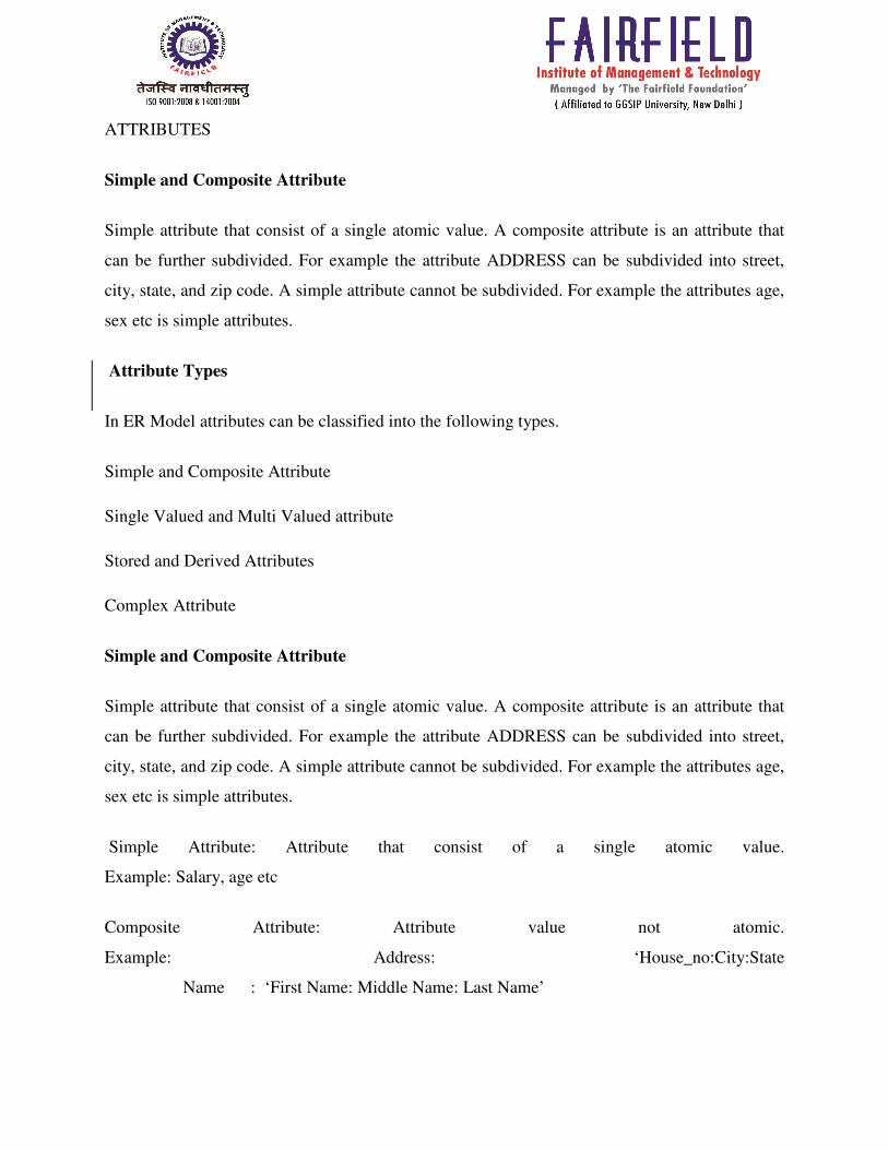
Simple and Composite Attribute

Simple attribute that consist of a single atomic value. A composite attribute is an attribute that

can be further subdivided. For example the attribute ADDRESS can be subdivided into street,

city, state, and zip code. A simple attribute cannot be subdivided. For example the attributes age,

sex etc is simple attributes.

Attribute Types

In ER Model attributes can be classified into the following types.


Single Valued and Multi Valued attribute

Stored and Derived Attributes

Complex Attribute


Simple attribute that consist of a single atomic value. A composite attribute is an attribute that

can be further subdivided. For example the attribute ADDRESS can be subdivided into street,

city, state, and zip code. A simple attribute cannot be subdivided. For example the attributes age,

sex etc is simple attributes.

Simple Attribute: Attribute that consist of a single atomic value.

Example: Salary, age etc

Composite Attribute: Attribute value not atomic.

Example: Address: ‘House_no:City:State

Name : ‘First Name: Middle Name: Last Name’

Single Valued and Multi Valued attribute

A single valued attribute can have only a single value. For example a person can have only one

'date of birth', 'age' etc. That is a single valued attributes can have only single value. But it can be

simple or composite attribute. That is 'date of birth' is a composite attribute , 'age' is a simple

attribute. But both are single valued attributes. Single Valued Attribute: Attribute that hold a

single value

Multivalve attributes can have multiple values. For instance a person may have multiple

phone numbers, multiple degrees etc.Multivalued attributes are shown by a double line

connecting to the entity in the ER diagram. Attributes (like phone numbers) that are

explicitly repeated in a class definition aren’t the only design problem that we might have to

correct. Suppose that we want to know what hobbies each person on our contact list is

interested in (perhaps to help us pick birthday or holiday presents). We might add an

attribute to hold these. More likely, someone else has already built the database, and added

this attribute without thinking about it.

Example for single value attributes1: Age

Exampe2: City

Example3: Customer id

Multi Valued Attribute: Attribute that hold multiple values.

Example1: A customer can have multiple phone numbers, email id's etc

Example2: A person may have several college degrees

Stored and Derived Attributes

The value for the derived attribute is derived from the stored attribute. For example 'Date of

birth' of a person is a stored attribute. The value for the attribute 'AGE' can be derived by

subtracting the 'Date of Birth'(DOB) from the current date. Stored attribute supplies a value to

the related attribute.

Stored attributes:

The stored attribute are such attributes which are already stored in the database and from which

the value of another attribute is derived is called stored attribute. For example age of a person

can be calculated from person’s date of birth and present date. Difference between these two

dates gives the value of age. In this case, date of birth is a stored attribute and age of the person

is the derived attribute

Derived attributes: The derived attributes are such attributes for which the value is derived or

calculated from stored attributes. For example date of birth of an employee is the stored attribute

but the age is the derived attributed. Derived attributes are usually created by a formula or by a

summary operation on other attributes.

Relationship:-

A relationship, in the context of databases, is a situation that exists between two relational

database tables when one table has a foreign key that references the primary key of the other

table. Relationships allow relational databases to split and store data in different tables, while

linking disparate data items. For example, in a bank database a CUSTOMER_MASTER table

stores customer data with a primary key column named CUSTOMER_ID; it also stores customer

data in an ACCOUNTS_MASTER table, which holds information about various bank accounts

and associated customers. To link these two tables and determine customer and bank account

information, a corresponding CUSTOMER_ID column must be inserted in the

ACCOUNTS_MASTER table, referencing existing customer ids from the

CUSTOMER_MASTER table. In this case, the ACCOUNTS_MASTER table’s

CUSTOMER_ID column is a foreign key that references a column with the same name in the

CUSTOMER_MASTER table. This is an example of a relationship between the two tables.

Relation Types :-

After two or more entities are identified and defined with attributes, the participants Determine if

a relationship exists between the entities. A relationship is any association, linkage, or

connection between the entities of interest to the business; it is a two-directional, significant

association between two entities, or between an entity and itself. Each relationship has a name,

an optionality (optional or mandatory), and a degree (how many). A relationship is described in

real terms. Assigning a name, optionality, and a degree to a relationship helps confirm the

validity of that relationship. If you cannot give a relationship all these things, then perhaps

thermally is no relationship at all.

Relationship represents an association between two or more entities. An example of relationship

would be

Employees are assigned to projects

Projects have subtasks

Departments manage one or more projects

Relationships are the connections and interactions between the entities instances e.g.

DEPT_EMP associates Department and Employee.

A relationship type is an abstraction of a relationship i.e. a set of relationships instances sharing

common attributes.

Entities enrolled in a relationship are called its participants.

The participation of an entity in a relationship is total when all entities of that set might

be participant in the relationship otherwise it is partial e.g. if every Part is supplied by a

Supplier then the SUPP_PART relationship is total. If certain parts are available without

a supplier than it is partial.

Naming Relationships:

If there is no proper name of the association in the system then participants' names of

Abbreviations are used. STUDENT and CLASS have ENROLL relationship. However, it

Can also be named as STD_CLS.

Roles:

Entity set of a relationship need not be distinct. For example

Phone,Name,City,SSN,Manager,Employee,Works-for,Worker

The labels "manager" and "worker" are called "roles". They specify how employee Entities

interact via the "works-for" relationship set. Roles are indicated in

ER diagrams by labeling the lines that connect diamonds to rectangles. Roles are optional. They

clarify semantics of a relationship. Symbol for Relationships: Participants are connected by

continuous lines, labeled to indicate cardinality. In partial relationships roles (if identifiable) are

written on the line connecting the.

Weak Entity: - In a relational database, a weak entity is an entity that cannot be uniquely

identified by its attributes alone; therefore, it must use a foreign key in conjunction with its

attributes to create a primary key. The foreign key is typically a primary key of an entity it is

related to.In entity relationship diagrams a weak entity set is indicated by a bold (or double-

lined) rectangle (the entity) connected by a bold (or double-lined) type arrow to a bold (or

double-lined) diamond (the relationship). This type of relationship is called an identifying

relationship and in IDEF1X notation it is represented by an oval entity rather than a square entity

for base tables. An identifying relationship is one where the primary key is populated to the child

weak entity as a primary key in that entity.

In general (though not necessarily) a weak entity does not have any items in its primary key

other than its inherited primary key and a sequence number. There are two types of weak

entities: associative entities and subtype entities.

RELATIONSHIPS

After two or more entities are identified and defined with attributes, the participants determine if

a relationship exists between the entities. A relationship is any association, Linkage, or

connection between the entities of interest to the business; it is a two-Directional, significant

association between two entities, or between an entity and itself.

Each relationship has a name, an optionality (optional or mandatory), and a degree (how many).

A relationship is described in real terms. Assigning a name, optionality, and a degree to a

relationship helps confirm the validity of

that relationship. If you cannot give a relationship all these things, then perhaps there really is no

relationship at all Relationship works by matching data in key columns — usually columns with

the same name in both tables. In most cases, the relationship matches the primary key from one

table, which provides a unique identifier for each row, with an entry in the foreign key in the

other table. For example, book sales can be associated with the specific titles sold by creating a

relationship between the title_id column in the titles table (the primary key) and the title_id

column in the sales table (the foreign key).

There are three types of relationships between tables. The type of relationship that is created

depends on how the related columns are defined.

One-to-Many Relationships

Many-to-Many Relationships

One-to-One Relationship

One-to-Many Relationships

One-To-Many Relationship:--A one-to-many relationship is the most common type of

relationship. In this type of relationship, a row in table A can have many matching rows in table

B, but a row in table B can have only one matching row in table A. For example, the publishers

and titles tables have a one-to-many relationship: each publisher produces many titles, but each

title comes from only one publisher. Make a one-to-many relationship if only one of the related

columns is a primary key or has a unique constraint. The primary key side of a one-to-many

relationship is denoted by a key symbol. The foreign key side of a relationship is denoted by an

infinity symbol.

Many-To-Many Relationship:- In a many-to-many relationship, a row in table A can have

many matching rows in table B, and vice versa. You create such a relationship by defining a

third table, called a junction table, whose primary key consists of the foreign keys from both

table A and table B. For example, the authors table and the titles table have a many-to-many

relationship that is defined by a one-to-many relationship from each of these tables to the title

authors table. The primary key of the title authors table is the combination of the au_id column

(the authors table's primary key) and the title_id column (the titles table's primary key).

One-To-One Relationship: In a one-to-one relationship, a row in table A can have no more

than one matching row in table B, and vice versa. A one-to-one relationship is created if both of

the related columns are primary keys or have unique constraints.

This type of relationship is not common because most information related in this way would be

all in one table. You might use a one-to-one relationship to:

Divide a table with many columns.

Isolate part of a table for security reasons.

Store data that is short-lived and could be easily deleted by simply deleting the table.

Store information that applies only to a subset of the main table.

The primary key side of a one-to-one relationship is denoted by a key symbol. The foreign key

side is also denoted by a key symbol.

Enhanced (Extended) ER Diagrams

Contain all the basic modeling concepts of an ER Diagram

Adds additional concepts:

Specialization/generalization

Subclass/super class

Categories

Attribute inheritance

Extended ER diagrams use some object

EER is used to model concepts more accurately than the ER diagram.

Sub classes and Super classes

In some cases, and entity type has numerous sub

and need to be explicitly represented, because of their importance.

For example, members of entity Employee can be grouped further into Secretary, Engineer,

Manager, Technician, Salaried Employee

The set listed is a subset of the entities that

every entity that belongs to one of the sub sets is also an Employee.

Each of these sub-groupings is called a subclass, and the Employee entity is called the super

nded ER diagrams use some object-oriented concepts such as inheritance.

EER is used to model concepts more accurately than the ER diagram.

In some cases, and entity type has numerous sub-groupings of its entities that are

and need to be explicitly represented, because of their importance.


Salaried Employee.

The set listed is a subset of the entities that belong to the Employee entity, which means that

every entity that belongs to one of the sub sets is also an Employee.

groupings is called a subclass, and the Employee entity is called the super

groupings of its entities that are meaningful,


belong to the Employee entity, which means that

groupings is called a subclass, and the Employee entity is called the super-

Employee

Secretary Technician Engineer

d

Work Department

class.

An entity cannot only be a member of a subclass; it must also be a member of the super-class.

An entity can be included as a member of a number of sub classes, for example, a Secretary may

also be a salaried employee, however not every member of the super class must be a member of

a sub class.

Type Inheritance

The type of an entity is defined by the attributes it possesses, and the relationship types it

participates in.

Because an entity in a subclass represents the same entity from the super class, it should possess

all the values for its attributes, as well as the attributes as a member of the super class.This means

that an entity that is a member of a subclass inherits all the attributes of the entity as a member of

the super class; as well, an entity inherits all the relationships in which the super class

participates.

Specialization

The process of defining a set of subclasses of a super class.

Specialization is the top-down refinement into (super) classes and subclasses

The set of sub classes is based on some distinguishing characteristic of the super class.

For example, the set of sub classes for Employee, Secretary, Engineer, Technician, differentiates

among employee based on job type.

There may be several specializations of an entity type based on different distinguishing

characteristics.

Another example is the specialization, Salaried Employee and Hourly_Employee, which

distinguish employees based on their method of pay.

Notation for Specialization

To represent a specialization, the subclasses that define a specialization are attached by lines to a

circle that represents the specialization, and is connected to the super class. The subset symbol

(half-circle) is shown on each line connecting a subclass to a super class, indicates the direction

of the super class/subclass relationship. Attributes that only apply to the sub class are attached to

the rectangle representing the subclass. They are called specific attributes.

A sub class can also participate in specific relationship types. See Example.

Employee

Secretary Technician Engineer

d

Work Department

Belong

s To

Professional

Organization

Reasons for Specialization

Certain attributes may apply to some but not all entities of a super class. A subclass is defined in

order to group the entities to which the attributes apply.

The second reason for using subclasses is that some relationship types may be participated in

only by entities that are members of the subclass.

Summary of Specialization

Allows for:

Defining set of subclasses of entity type, Create additional specific attributes for each sub class,

Create additional specific relationship types between each sub class and other entity types or

other subclasses.

Generalization: - A generalization (or generalization) of a concept is an extension of the

concept to less-specific criteria. It is a foundational element of logic and human reasoning

.Generalizations posit the existence of a domain or set of elements, as well as one or more

common characteristics shared by those elements. As such, they are the essential basis of all

valid deductive inferences. The process of verification is necessary to determine whether a

generalization holds true for any given situation.

The concept of generalization has broad application in many related disciplines, sometimes

having a specialized context or meaning.

The reverse of specialization is generalization.

Several classes with common features are generalized into a super class.

For example, the entity types Car and Truck share common attributes License_PlateNo, Vehicle

and Price, therefore they can be generalized into the super class Vehicle.

Constraints on Specialization and Generalization

Several specializations can be defined on an entity

each of the specializations. The

manager specialization; in this case we don’t use the circle notation.

Types of Specializations

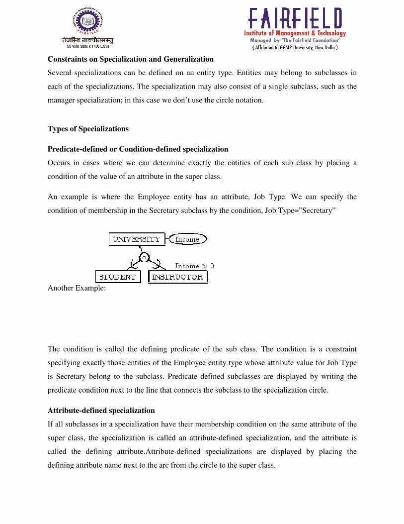
Predicate-defined or Condition

Occurs in cases where we can determine exactly the entities of each sub class by placing a

condition of the value of an attribute in the super class.

An example is where the Employee entity has an attribute, Job Type. We can specify the

condition of membership in the Secretary subclass by the condition, Job Type=”Secretary”

Another Example:

The condition is called the defining predicate of the sub

specifying exactly those entities of the Employee entity type whose attribute value for Job Type

is Secretary belong to the subclass. Predicate

predicate condition next to the line that connects the subclass to the specialization circle.

Attribute-defined specialization

If all subclasses in a specialization have their membership condition on the same attribute of the

super class, the specialization is called an attribute

called the defining attribute.Attribute

defining attribute name next to the arc from the circle to the super class.

Constraints on Specialization and Generalization

Several specializations can be defined on an entity type. Entities may belong to subclasses in

specialization may also consist of a single subclass, such as the

alization; in this case we don’t use the circle notation.

defined or Condition-defined specialization


attribute in the super class.



defining predicate of the sub class. The condition is a constraint


subclass. Predicate defined subclasses are displayed by writing t


defined specialization


tion is called an attribute-defined specialization, and the attribute is

called the defining attribute.Attribute-defined specializations are displayed by placing the

defining attribute name next to the arc from the circle to the super class.

may belong to subclasses in

specialization may also consist of a single subclass, such as the




condition is a constraint


defined subclasses are displayed by writing the



defined specialization, and the attribute is

defined specializations are displayed by placing the

User-defined specialization

When we do not have a condition for determining membership in a subclass the subclass is

called user-defined. Membership to a subclass is determined by the database users when they add

an entity to the subclass.

Disjointness/Overlap Constraint

Specifies that the subclass of the specialization must be disjoint, which means that an entity can

be a member of, at most, one subclass of the specialization. The d in the specialization circle

stands for disjoint. If the subclasses are not constrained to be disjoint, they overlap. Overlap

means that an entity can be a member of more than one subclass of the specialization. Overlap

constraint is shown by placing an o in the specialization circle.

Completeness Constraint

The completeness constraint may be either total or partial.

A total specialization constraint specifies that every entity in the super class must be a member

of at least one subclass of the specialization.Total specialization is shown by using a double line

to connect the super class to the circle.A single line is used to display a partial specialization,

meaning that an entity does not have to belong to any of the subclasses.

Disjointness vs. Completeness

Disjoint constraints and completeness constraints are independent. The following possible

constraints on specializations are possible:

Disjoint, total

Department

d

Academic Administrative

Disjoint, partial

Overlapping, total

Employee

d

Secretary Analyst Engineer

Part

o

Manufactured Puchased

UNIT – II

INTRODUCTION TO SQL:

Overview: - SQL is a standard language for accessing and manipulating databases. SQL stands

for Structured Query Language,SQL lets you access and manipulate databases,SQL is an ANSI

(American National Standards Institute) standard. SQL stands for Structured Query Language.

SQL language is used to create, transform and retrieve information from RDBMS (Relational

Database Management Systems). SQL is pronounced SEQUEL. SQL was developed during the

early 70’s at IBM. Most Relational Database Management Systems like MS SQL Server,

Microsoft Access, Oracle, MySQL, DB2, Sybase, PostgreSQL and Informix use SQL as a

database querying language. Even though SQL is defined by both ISO and ANSI there are many

SQL implementation, which do not fully comply with those definitions. Some of these SQL

implementations are proprietary. Examples of these SQL dialects are MS SQL Server specific

version of the SQL called T-SQL and Oracle version of SQL called PL/SQL.SQL is a declarative

programming language designed for creating and querying relational database management

systems. SQL is relatively simple language, but it’s also very powerful.SQL can insert data into

database tables. SQL can modify data in existing database tables. SQL can delete data from SQL

database tables. Finally SQL can modify the database structure itself – create/modify/delete

tables and other database objects.

Characteristics of SQL

SQL can execute queries against a database

SQL can retrieve data from a database

SQL can insert records in a database

SQL can update records in a database

SQL can delete records from a database

SQL can create new databases

SQL can create new tables in a database

SQL can create stored procedures in a database

SQL can create views in a database

SQL can set permissions on tables, procedures, and views.

Advantages of SQL:

* High Speed:

SQL Queries can be used to retrieve large amounts of records from a database quickly and

efficiently.

* Well Defined Standards Exist: SQL databases use long-established standard, which is being

adopted by ANSI & ISO. Non-SQLdatabases do not adhere to any clear standard.

* No Coding Required:

Using standard SQL it is easier to manage database systems without having to write substantial

amount of code.

* Emergence of ORDBMS: Previously SQL databases were synonymous with relational

database. With the emergence of Object-oriented DBMS, object storage capabilities are extended

to relational databases.

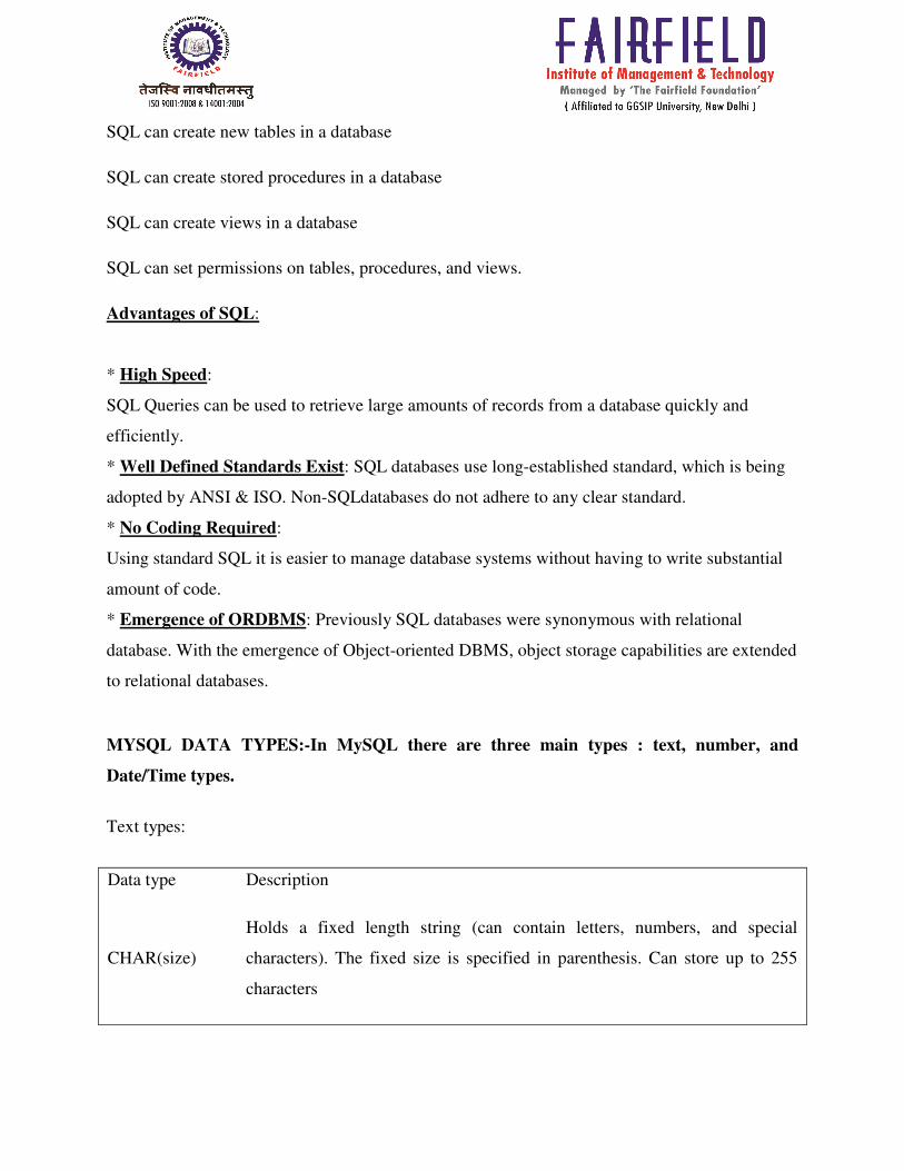
MYSQL DATA TYPES:-In MySQL there are three main types : text, number, and

Date/Time types.

Text types:

Data type Description

CHAR(size)

Holds a fixed length string (can contain letters, numbers, and special

characters). The fixed size is specified in parenthesis. Can store up to 255

characters

VARCHAR(size)

Holds a variable length string (can contain letters, numbers, and special

characters). The maximum size is specified in parenthesis. Can store up to

255 characters. Note: If you put a greater value than 255 it will be converted

to a TEXT type

TINYTEXT Holds a string with a maximum length of 255 characters

TEXT Holds a string with a maximum length of 65,535 characters

BLOB For BLOBs (Binary Large Objects). Holds up to 65,535 bytes of data

MEDIUMTEXT Holds a string with a maximum length of 16,777,215 characters

MEDIUMBLOB For BLOBs (Binary Large Objects). Holds up to 16,777,215 bytes of data

LONGTEXT Holds a string with a maximum length of 4,294,967,295 characters

LONGBLOB For BLOBs (Binary Large Objects). Holds up to 4,294,967,295 bytes of data

ENUM(x, y,z,etc.)

Let you enter a list of possible values. You can list up to 65535 values in an

ENUM list. If a value is inserted that is not in the list, a blank value will be

inserted.

Note: The values are sorted in the order you enter them.

You enter the possible values in this format: ENUM('X','Y','Z')

SET Similar to ENUM except that SET may contain up to 64 list items and can

store more than one choice

Types of SQL commands: DDL, DML, DCL.

DDL

Data Definition Language (DDL) statements are used to define the database structure or

schema. They are called data definition since they are used for defining the data. That is the

structure of the data is known through these DDL commands.

.Some examples:

CREATE - to create objects in the database

ALTER - alters the structure of the database

DROP - delete objects from the database

TRUNCATE - remove all records from a table, including all spaces allocated for the records are

removed

COMMENT - add comments to the data dictionary

RENAME - rename an object

DML

Data Manipulation Language (DML) statements are used for managing data within schema

objects. DML statements can be roll backed where DDL are auto commit. DML commands are

used for data manipulation. Some of the DML commands

insert, select, update, delete etc. Even though select is not exactly a DML language command

oracle still recommends you to consider SELECT as a DML command some examples:

SELECT - retrieve data from the a database

INSERT - insert data into a table

UPDATE - updates existing data within a table

DELETE - deletes all records from a table, the space for the records remain

MERGE - UPSERT operation (insert or update)

CALL - call a PL/SQL or Java subprogram

EXPLAINS PLAN - explain access path to data

LOCK TABLE - control concurrency

DCL

Data Control Language (DCL) Data Control Language is used for the control of data. That is a

user can access any data based on the privileges given to him. This is done through DATA

CONTROL LANGUAGE. Some of the DCL Commands are:

1. GRANT

2. REVOKE... Some examples:

GRANT - gives user's access privileges to database

REVOKE - withdraw access privileges given with the GRANT command

BASIC SQL QUIRES:

Basic SQL Components

SELECT schema.table.column

FROM table alias

WHERE [conditions]

ORDER BY [columns]

Defines the end of an SQL statement Defines statement Some programs require it, some do not

(TOAD Does Not).Needed only if multiple SQL statements run in a script Needed script.

SELECT Statement

SELECT Statement Defines WHAT is to be returned (separated by commas)

Database Columns (From Tables or Views)

Constant Text Values Constant Values

Formulas

PrePre-defined Functions

Group Functions (COUNT, SUM, MAX, MIN, AVG)

““*” Mean All Columns from All Tables In the

FROM Statement

Example: SELECT state code, state name from employee; Example: name

FROM STATEMENT

Defines the Table(s) or View(s) Used by the SELECT or WHERE Statements the

Statements

You MUST Have a FROM statement you statement

Multiple Tables/Views are separated by Commas.

EXAMPLE :

SELECT state_name, state_code from record;

SELECT DISTINCT Example

The following SQL statement selects only the distinct values from the "City" columns from the

"Customers" table:

Example

SELECT DISTINCT City FROM Customers;

The SQL WHERE Clause

The WHERE clause is used to extract only those records that fulfill a specified criterion.

SQL WHERE Syntax

1. SELECT column name, column name

FROM table name WHERE column name operator value

2. SELECT * FROM Customers WHERE Customer=1;

3. SQL aliases are used to give a database table or a column in a table, a temporary name.

Basically aliases are created to make column names more readable.

SQL Alias Syntax for Columns

SELECT column name AS alias name FROM table name AND OPITION WITH EXAMPLE.

SELECT * FROM Customers WHERE Country='Germany' AND City='Berlin'

Logical operators: BETWEEN, IN, AND, OR and NOT

There are three Logical Operators namely, AND, OR, and NOT. These operators compare two

conditions at a time to determine whether a row can be selected for the output. When retrieving

data using a SELECT statement, you can use logical operators in the WHERE clause, which

allows you to combine more than one condition.

Logical

Operators Description

OR For the row to be selected at least one of

the conditions must be true.

AND For a row to be selected all the specified

conditions must be true.

NOT For a row to be selected the specified

condition must be false.

"AND" Logical Operator:

If you want to select rows that must satisfy all the given conditions, you can use the logical

operator, AND.

For Example: To find the names of the students between the age 10 to 15 years, the query

would be like:

SELECT first name, last-named, age FROM student details WHERE age >= 10 AND age

<= 15;

"NOT" Logical Operator:

If you want to find rows that do not satisfy a condition, you can use the logical operator, NOT.

NOT results in the reverse of a condition. That is, if a condition is satisfied, then the row is not

returned.

For example: If you want to find out the names of the students who do not play football, the

query would be like:

SELECT first name, last-name, games FROM student details WHERE NOT games =

'Football'

Concept of null values: Users new to the world of databases are often confused by a special

value particular to our field – the NULL value. This value can be found in a field containing any

type of data and has a very special meaning within the context of a relational database. It’s

probably best to begin our discussion of NULL with a few words about what NULL is not:

NULL is not the number zero.

NULL is not the empty string (“”) value.

Rather, NULL is the value used to represent an unknown piece of data. Let’s take a look at a

simple example: a table containing the inventory for a fruit stand. Suppose that our

inventory contains 10 apples, 3 oranges. We also stock plums, but our inventory information

is incomplete and we don’t know how many (if any) plums are in stock. Using the NULL

value, we would have the inventory table shown at the bottom of this page.

Comparisons with NULL value: - Since Null is not a member of any data domain, it is not

considered a "value", but rather a marker (or placeholder) indicating the absence of value.

Because of this, comparisons with Null can never result in either True or False, but always in a

third logical result, Unknown. And assume the rules of NULLs:

NULL = NULL evaluates to unknown

NULL <> NULL evaluates to unknown

Value = NULL evaluates unknown

Any comparison with NULL yields NULL. To overcome this, there are three operators you can

use:

x IS NULL - determines whether left hand expression is NULL,

x IS NOT NULL - like above, but the opposite,

x <=> y - compares both operands for equality in a safe manner, i.e. NULL is seen as a

normal value.

For your code, you might want to consider using the third option and go with the null safe

comparison:

SELECT * FROM my compare

WHERE NOT (name <=> fname OR name <=> mname OR name <=> lname).

SQL Integrity Constraints

Integrity Constraints are used to apply business rules for the database tables.

The constraints available in SQL are Foreign Key, Not Null, Unique, Check.

Constraints can be defined in two ways

1) the constraints can be specified immediately after the column definition. This is called

column-level definition.

2) The constraints can be specified after all the columns are defined. This is called table-level

definition.

1) SQL Primary key:

This constraint defines a column or combination of columns which uniquely identifies each row

in the table.

Syntax to define a Primary key at column level:

column name data type [CONSTRAINT constraint_name] PRIMARY KEY

Syntax to define a Primary key at table level:

[CONSTRAINT constraint_name] PRIMARY KEY (column_name1, column_name2,..)

• column_name1, column_name2 are the names of the columns which define the

primary Key.

• The syntax within the bracket i.e. [CONSTRAINT constraint name] is optional.

2. SQL Foreign key or Referential Integrity:

This constraint identifies any column referencing the PRIMARY KEY in another table. It

establishes a relationship between two columns in the same table or between different tables. For

a column to be defined as a Foreign Key, it should be a defined as a Primary Key in the table

which it is referring. One or more columns can be defined as Foreign key.

Syntax to define a Foreign key at column level:

[CONSTRAINT constraint name] REFERENCES Referenced_Table_name (column

name) Syntax to define a Foreign key at table level:

[CONSTRAINT constraint name] FOREIGN KEY(column name) REFERENCES

referenced_table_name(column name);

3. SQL Not Null Constraint:

This constraint ensures all rows in the table contain a definite value for the column which is

specified as not null. Which means a null value is not allowed.

Syntax to define a Not Null constraint:

[CONSTRAINT constraint name] NOT NULL

4. SQL Unique Key constraints:

This constraint ensures that a column or a group of columns in each row have a distinct value. A

column(s) can have a null value but the values cannot be duplicated.

Syntax to define a unique key at column level:

[CONSTRAINT constraint name] UNIQUE

Syntax to define a Unique key at table level:

[CONSTRAINT constraint name] UNIQUE (column name)

5. SQL Check Constraint:

This constraint defines a business rule on a column. All the rows must satisfy this rule. The

constraint can be applied for a single column or a group of columns.

Syntax to define a Check constraint:

[CONSTRAINT constraint name] CHECK (condition

Introduction to Nested Queries, Correlated Nested Queries:-

A sub query is a query that is nested inside a SELECT, INSERT, UPDATE, or DELETE

statement, or inside another sub query. A sub query can be used anywhere an expression is

allowed. In this example a sub query is used as a column expression named MaxUnitPrice in a

SELECT statement. A sub query is also called an inner query or inner select, while the statement

containing a sub query is also called an outer query or outer select.

Many Transact-SQL statements that include sub queries can be alternatively formulated as joins.

Other questions can be posed only with sub queries. In Transact-SQL, there is usually no

performance difference between a statement that includes a sub query and a semantically

equivalent version that does not. However, in some cases where existence must be checked, a

join yields better performance. Otherwise, the nested query must be processed for each result of

the outer query to ensure elimination of duplicates. In such cases, a join approach would yield

better results. The following is an example showing both a sub query SELECTS and a join

SELECT that return the same result set:

Example: /* SELECT statement built using a sub query. */

SELECT Name

FROM AdventureWorks2008R2.Production.Product

WHERE List Price =

(SELECT List Price

FROM AdventureWorks2008R2.Production.Product

WHERE Name = 'Chaining Bolts’);

Nested Sub query:-If a Sub query contains another sub query, then the sub query inside another

sub query is called nested sub query.

Let us suppose we have another table called “Student Course” which contains the information,

which student is connected to which Course. The structure of the table is:-

create table Student Course( StudentCourseid int identity(1,1), Student int, Coursed into)

The Query to insert data into the table “Student course” is

Insert into Student Course values (1, 3)




Note: - We don’t need to insert data for the column Student Course id since it is an identity

column.

Now, if we want to get the list of all the student which belong to the

Correlated Sub query:-If the outcome of a sub query is depends on the value of a column of its

parent query table then the Sub query is called Correlated Sub query.

Suppose we want to get the details of the Courses (including the name of their course admin)

from the Course table, we can use the following query:-

select Course name ,Course admin id,(select First name+' '+Last name from student where

student id=Course. Course admin id)as CourseAdminName from course

It is not necessary that the column on which the correlated query is depended is included in the

selected columns list of the parent query.

SQL Comparison Operators:- Comparison operators test whether two expressions are the same.

Comparison operators can be used on all expressions except expressions of the text, n text, or

image data types. The following table lists the Transact-SQL comparison operators.

Operator Description Example

=

Checks if the value of two operands is

equal or not, if yes then condition

becomes true.

(a = b) is not true.

!=

Checks if the value of two operands is

equal or not, if values are not equal then

condition becomes true.

(a != b) is true.

<> Checks if the value of two operands is (a <> b) is true.

equal or not, if values are not equal then


>

Checks if the value of left operand is

greater than the value of right operand, if

yes then condition becomes true.

(a > b) is not true.

<

Checks if the value of left operand is less

than the value of right operand, if yes then


(a < b) is true.

>=

Checks if the value of left operand is

greater than or equal to the value of right

operand, if yes then condition becomes

true.

(a >= b) is not true.

<=

Checks if the value of left operand is less

than or equal to the value of right operand,

if yes then condition becomes true.

(a <= b) is true.

!<

Checks if the value of left operand is not

less than the value of right operand, if yes

then condition becomes true.

(a !< b) is false.

!>

Checks if the value of left operand is not

greater than the value of right operand, if

yes then condition becomes true.

(a !> b) is true

Aggregate functions:-

Aggregate functions perform a calculation on a set of values and return a single value. Except for

COUNT, aggregate functions ignore null values. Aggregate functions are frequently used with

the GROUP BY clause of the SELECT statement.

All aggregate functions are deterministic. This means aggregate functions return the same value

any time that they are called by using a specific set of input values. For more information about

function determinism, see Deterministic and Nondeterministic Functions. The OVER clause may

follow all aggregate functions except GROUPING and GROUPING_ID.

Aggregate functions can be used as expressions only in the following:

• The select list of a SELECT statement (either a sub query or an outer query).

• A HAVING clause.

• The group by clauses.

• The SQL GROUP BY is a clause enables SQL aggregate functions for a grouping of

information. For example, it could support subtotaling by region number in a sales table.

The SQL GROUP BY is a clause enables SQL aggregate functions for a grouping of information. For

example, it could support subtotaling by region number in a sales table. GROUP BY supports dividing

data into sets so that aggregate functions like SUM, AVG and COUNT can be performed. The SQL

GROUP BY clause is used whenever aggregate functions by group are required. This is an aid to

understanding and analyzing information.

SQL GROUP BY is used as follows. It must follow the FROM and WHERE clauses. The columns in a

SELECT clause must be either group by columns or aggregate function columns.

SQL GROUP BY Syntax :- SELECT <column_name1>, <column_name2> <aggregate function>

FROM <table name>

GROUP BY <column_name1>, <column_name2>

Joins: Inner joins, Outer Joins, Left outer, Right outer, full outer joins :-

The SQL JOIN is a clause that enables a SELECT statement to access more than one table. The JOIN

clause controls how tables are linked. It is a qualifier of the SQL FROM clause. The standard JOIN

clause (also known as the INNER JOIN clause) differs from the OUTER JOIN in that rows are returned

only when there are matches for the JOIN criteria on the second table. Use the SQL JOIN whenever

multiple tables must be accessed through a SQL SELECT statement and no results should be returned if

there is not a match between the Joined tables.

SQL JOIN is used as follows. The ON clause describes the conditions of the JOIN.

Important! A "Cartesian product" can result if there is no relating the tables for the join. A row would

be included for each combination between the two tables so if one table has 1,000 rows and the second

table has 2,000 rows then 2,000,000 rows would be returned. An SQL JOIN clause is used to combine

rows from two or more tables, based on a common field between them.

The most common type of join is: SQL INNER JOIN (simple join). An SQL INNER JOIN return all

rows from multiple tables where the join condition is met

Important! If there are no matches on the JOIN criteria then no rows will be returned. This is known an

"INNER JOIN". Use the "OUTER JOIN" in cases where rows should be returned when one side of the

join is missing.

SQL JOIN Syntax :- SELECT <column_name1>, <column_name2> <aggregate function>

FROM <table name>

JOIN <table_name> ON <join conditions>

Inner joins: - The INNER JOIN keyword selects all rows from both tables as long as there is a match

between the columns in both tables. The INNER JOIN keyword selects all rows from both tables as long

as there is a match between the columns. The most frequently used and important of the joins is the

INNER JOIN. They are also referred to as an EQUIJOIN.

The INNER JOIN creates a new result table by combining column values of two tables (table1 and

table2) based upon the join-predicate. The query compares each row of table1 with each row of table2 to

find all pairs of rows which satisfy the join-predicate. When the join-predicate is satisfied, column

values for each matched pair of rows of A and B are combined into a result row.

Syntax: - SELECT table1.column1, table2.column2...

FROM table1

INNER JOIN table2

ON table1.common_filed = table2.common_field;

OUTER JOINING : The SQL OUTER JOIN clause is a variation of the SQL JOIN clause enables a

SELECT statement to access more than one table. The JOIN clause controls how tables are linked. It is a

qualifier of the SQL FROM clause. The OUTER JOIN clause differs from the standard JOIN clause

(also known as the INNER JOIN clause) in that rows are returned even when there are no matches

through the JOIN criteria on the second table.

Use the SQL OUTER JOIN whenever multiple tables must be accessed through a SQL SELECT

statement and results should be returned if there is not a match between the Joined tables. It can be

useful when there is a need to merge data from two tables and to include all rows from both tables

without depending on a match. Another use is to generate a large result set for testing purposes.

Syntax for outer joining :

SELECT <column_name1>,

<column_name2> <aggregate_function>

FROM <table_name>

LEFT OUTER JOIN <table_name> ON <join_conditions>

Left outer, Right outer, full outer joins: - A SQL join clause combines records from two or more

tables in a database . It creates a set that can be saved as a table or used as it is. A JOIN is a means

for combining fields from two tables by using values common to each. ANSI standard SQL specifies

four types of JOIN : INNER , OUTER , LEFT , and RIGHT . As a special case, a table

(base table, view, or joined table) can JOIN to itself in a self-join. A programmer writes a JOIN

statement to identify the records for joining. If the evaluated predicate is true, the combined record is

then produced in the expected format, a record set or a temporary table.

Outer join

An outer join does not require each record in the two joined tables to have a matching record. The

joined table retains each record—even if no other matching record exists. Outer joins subdivide further

into left outer joins, right outer joins, and full outer joins, depending on which table's rows are retained

(left, right, or both).

(In this case left and right refer to the two sides of the JOIN keyword.)

No implicit join-notation for outer joins exists in standard SQL.

Left outer join

The result of a left outer join (or simply left join) for table A and B always contains all records of the

"left" table (A), even if the join-condition does not find any matching record in the "right" table (B).

This means that if the ON clause matches 0 (zero) records in B (for a given record in A), the join

will still return a row in the result (for that record)—but with NULL in each column from B. A left

outer join returns all the values from an inner join plus all values in the left table that do not match to

the right table. For example, this allows us to find an employee's department, but still shows the

employee(s) even when they have not been assigned to a department (contrary to the inner-join example

above, where unassigned employees were excluded from the result

Example of left outer joining : SELECT *

FROM employee LEFT OUTER JOIN department

ON employee.DepartmentID = department.DepartmentID;

Right outer joining: A right outer join (or right join) closely resembles a left outer join, except with

the treatment of the tables reversed. Every row from the "right" table (B) will appear in the joined table

at least once. If no matching row from the "left" table (A) exists, NULL will appear in columns from A

for those records that have no match in B.

A right outer join returns all the values from the right table and matched values from the left table

(NULL in the case of no matching join predicate). For example, this allows us to find each employee

and his or her department, but still show departments that have no employees

Example :- SELECT *

FROM employee RIGHT OUTER JOIN department


Full outer joining :- Full outer join

Conceptually, a full outer join combines the effect of applying both left and right outer joins. Where

records in the FULL OUTER Joined tables do not match, the result set will have NULL values for every

column of the table that lacks a matching row. For those records that do match, a single row will be

produced in the result set (containing fields populated from both tables).

For example, this allows us to see each employee who is in a department and each department that has

an employee, but also see each employee who is not part of a department and each department which

doesn't have an employee.

Example full outer join:

SELECT *

FROM employee FULL OUTER JOIN department


UNIT – III

Relational Data Model: This topic provides an introduction to relational data models. The relational

data model was first introduced by Ted Codd of IBM Research in 1970. This topic provides an

understanding of what a relational model is, as well as how we might approach model development. The

purpose of the relational model is to provide a declarative method for specifying data and queries: users

directly state what information the database contains and what information they want from it, and let the

database management system software take care of describing data structures for storing the data and

retrieval procedures for answering queries.

.The relational model can be considered as having three parts and these are covered in sequence below:

1. Structural: defines the core of the data and the relationships involved. The model structure is

described in terms of relations, tuples, attributes and domains.

2. Manipulative: defines how the data in the model will be accessed and manipulated. This concerns

how relations in the model will be manipulated to produce other relations, which in turn provide the

answer to some question posed by a user of the data. The manipulation is achieved though relational

algebra or relational calculus.

3. Constraints: defines limits on the model. The constraints determine valid ranges and values of data

to be included in the model.

Relation: A relation comprises a set of tuples. Figure 3.1 is a tabular representation of the Student

relation containing five tuples. Relations have three important properties. Each relation has a name, a

cardinality and a degree. These properties help us to further define and describe relations. The three

properties introduced above are defined as follows.

Name: The first property is that a relation has a name which identifies it, for example the Student

relation illustrated in Figure 3.1.

2. Cardinality: The second property of a relation it its cardinality. This refers to the number of tuples in

the relation. If we again take Figure 3.1 as our example, then the cardinality of the Student relation is 5.

3. Degree: The third and final property of a relation is its degree. The degree of a relation refers to the

number of attributes in each tuple. Again, with reference to Figure 3.1, the degree of the Student relation

is 4, the attributes being MatricNo, Name, Registered and Counsellor

Tuple: A tuple is a sequence of attributes i.e. a row in the relation table. There are five tuples shown in

the Student relation in Figure 3.1 - the one highlighted concerns Student identified by the MatricNo

's07'.

Attribute: An attribute is a named column in the relation table. The Student relation in Figure 3.1

contains four attributes - the MatricNo attribute is highlighted, other attributes are Name, Registered and

Counsellor.

Domain: The domain construct is important as it identifies the type of an attribute. More formally the

domain is a named set of values which have a common meaning - the domain of an attribute defines the

set of values from which an attribute can draw. The domain of an attribute defines the set of values

which can apply to that attribute. The domain can be considered similar to the simple data types in

programming languages, such as int or char types in programming languages such as C++.

Domains are always atomic. This means that they have no structure. Figure 3.2 illustrates the example

domains relevant to the Student relation in Figure 3.1.

Matrices No’s = S01..S99

Person Names = string

Staff Nos = 1000..9999

Years = 1960..2040

The most important consequence of two attributes being defined on the same domain is that their

attribute values are comparable. It is important to make the distinction that two attributes are not

comparable if they have been declared in different domains, even if the underlying data type is the same.

For example, the underlying data type of both the Year and StaffNos domains is the basic data type int.

However, this does not mean that the Registered and Counsellor attributes are comparable. To attempt to

compare such attributes would not be meaningful.

characteristics of relations:

No Duplicate Tuples - A relation cannot contain two or more tuples which have the same values for all

the attributes. i.e., In any relation, every row is unique.

• Tuples are unordered - The order of rows in a relation is immaterial.

• Attributes are unordered - The order of columns in a relation is immaterial.

• Attribute Values are Atomic - Each tuple contains exactly one value for each attribute.

• Data in the relational database must be represented in tables, with values in columns within rows.

• Data within a column must be accessible by specifying the table name, the column name, and the

value of the primary key of the row.

• The DBMS must support missing and inapplicable information in a systematic way, distinct

from regular values and independent of data type.

• The DBMS must support an active on-line catalogue.

• The DBMS must support at least one language that can be used independently and from within

programs, and supports data definition operations, data manipulation, constraints, and transaction

management.

• Views must be updatable by the system.

• The DBMS must support insert, update, and delete operations on sets.

relational constraints domain constraints: Domain Constraints ,limit the range of domain values of an

attribute

specify uniqueness and `null ness' of an attribute specify a default value for an attribute when no value is

provided.

Entity Integrity .every tuple is uniquely identified by a unique non-null attributes the primary key.

Referential Integrity rows in different tables are correctly related by valid key values (`foreign' keys

refer to primary keys).

• Domain Constraints

o limit the range of domain values of an attribute

o specify uniqueness and `null ness' of an attribute

o Specify a default value for an attribute when no value is provided.

Relation constraints:- A table of values A relation may be thought of as a set of rows. Each row

represents a fact that corresponds to a Real-world entity or relationship. Each row has a value of an

item or set of items that Uniquely identifies that row in the table. Each column typically is called by its

column name or column header or attribute name.

Key of a Relation: Each row has a value of a data item (or set of items)

that uniquely identifies that row in the table Called the key. Sometimes row-ids or sequential numbers

are assigned as keys to identify the rows in a table Called artificial key or surrogate key.

A row is called a tuple, which is an ordered set of values A column header is called an attribute Each

attribute value is derived from an appropriate domain. The table is called a relation. A relation can be

regarded as a set of tuples (rows). The data type describing the types of values an attribute can have is

represented by a domain of possible values. Each row in the CUSTOMER table is a 4-tuple and consists

of four values.

A relation is a set of such tuples (rows). The relation is formed over the Cartesian product of

the sets; each set has values from a domain

• The Cartesian product of two sets A and B is defined

to be the set of all pairs (a, b) where a�A and b�B . It

is denoted A�B , and is called the Cartesian product

Key Constraints And Constraints On Null

SQL constraints are used to specify rules for the data in a table. If there is any violation between the

constraint and the data action, the action is aborted by the constraint. Constraints can be specified when

the table is created (inside the CREATE TABLE statement) or after the table is created (inside the

ALTER TABLE statement). SQL CREATE TABLE + CONSTRAINT Syntax:

CREATE TABLE table_name

(

column_name1 data_type(size) constraint_name,



....

);

In SQL, we have the following constraints:

• NOT NULL - Indicates that a column cannot store NULL value. The NOT NULL constraint

enforces a column to NOT accept NULL values. The NOT NULL constraint enforces a field to

always contain a value. This means that you cannot insert a new record, or update a record

without adding a value to this field.

The following SQL enforces the "P_Id" column and the "LastName" column to not accept NULL

values:

CREATE TABLE Persons

(

P_Id int NOT NULL,

LastName varchar(255) NOT NULL,

First Name varchar(255),

Address varchar(255),

City varchar(255)

)

UNIQUE - Ensures that each rows for a column must have a unique value. The UNIQUE constraint

uniquely identifies each record in a database table. The UNIQUE and PRIMARY KEY constraints both

provide a guarantee for uniqueness for a column or set of columns. A PRIMARY KEY constraint

automatically has a UNIQUE constraint defined on it. Note that you can have many UNIQUE

constraints per table, but only one PRIMARY KEY constraint per table.

Example:- CREATE TABLE Persons

(

P_Id int NOT NULL,




City varchar(255),

UNIQUE (P_Id)

)

PRIMARY KEY - A combination of a NOT NULL and UNIQUE. Ensures that a column (or

combination of two or more columns) have an unique identity which helps to find a particular record in

a table more easily and quickly. The PRIMARY KEY constraint uniquely identifies each record in a

database table. Primary keys must contain unique values. A primary key column cannot contain NULL

values. Each table should have a primary key, and each table can have only ONE primary key.

Example:- The following SQL creates a PRIMARY KEY on the "P_Id" column when the "Persons"

table is created:

value in a column meets a specific condition. The CHECK constraint is used to limit CREATE TABLE

Persons

(

P_Id int NOT NULL,




City varchar(255),

PRIMARY KEY (P_Id)

)

FOREIGN KEY - Ensure the referential integrity of the data in one table to match values in another

table. A FOREIGN KEY in one table points to a PRIMARY KEY in another table.

Let's illustrate the foreign key with an example. CREATE TABLE Orders

(

O_Id int NOT NULL,

Order No int NOT NULL,

P_Id int,

PRIMARY KEY (O_Id),

FOREIGN KEY (P_Id) REFERENCES Persons(P_Id)

)

CHECK - Ensures that the the value range that can be placed in a column. If you define a CHECK

constraint on a single column it allows only certain values for this column.If you define a CHECK

constraint on a table it can limit the values in certain columns based on values in other columns in the

row. The following SQL creates a check constraint on the "p_id" column when the "persons" table is

created. The check constraint specifies that the column "p_id" must only include integers greater than 0

Example: CREATE TABLE Persons

(

P_Id int NOT NULL,




City varchar(255),

CHECK (P_Id>0)

)

DEFAULT - Specifies a default value when specified none for this column. The DEFAULT constraint

is used to insert a default value into a column. The default value will be added to all new records, if no

other value is specified. The following SQL creates a DEFAULT constraint on the "City" column when

the "Persons" table is created:

CREATE TABLE Persons

(

P_Id int NOT NULL,




City varchar(255) DEFAULT 'Sandnes'

)

RELATION DB SCHEMA :- A database schema of a database system is its structure described in a

formal language supported by the database management system (DBMS) and refers to the organization

of data to create a blueprint of how a database will be constructed (divided into database tables). The

formal definition of database schema is a set of formulas (sentences) called integrity constraints imposed

on a database. These integrity constraints ensure compatibility between parts of the schema. All

constraints are expressible in the same language. A database can be considered a structure in realization

of the database language The states of a created conceptual schema are transformed into an explicit

mapping, the database schema. This describes how real world entities are modeled in the database.

"A database schema specifies, based on the database administrator's knowledge of possible applications,

the facts that can enter the database, or those of interest to the possible end-users." The notion of a

database schema plays the same role as the notion of theory in predicate calculus. A model of this

“theory” closely corresponds to a database, which can be seen at any instant of time as a mathematical

object. Thus a schema can contain formulas representing integrity constraints specifically for an

application and the constraints specifically for a type of database, all expressed in the same database

language] In a relational database, the schema defines the tables, fields, relationships, views, indexes,

packages, procedures, functions, queues, triggers, types, sequences, materialized views, synonyms,

database links, directories, XML schemas, and other elements.

Schemas are generally stored in a data dictionary. Although a schema is defined in text database

language, the term is often used to refer to a graphical depiction of the database structure. In other

words, schema is the structure of the database that defines the objects in the database

Levels of database schema:

• Conceptual schema, a map of concepts and their relationships.

• Logical schema, a map of entities and their attributes and relations.

• Physical schema, a particular implementation of a logical schema.

Codd's twelve rules

are a set of thirteen rules (numbered zero to twelve) proposed by Edgar F. Codd, a pioneer of the

relational model for databases, designed to define what is required from a database management system

in order for it to be considered relational, i.e., a relational database management system (RDBMS). They

are sometimes jokingly referred to as "Codd's Twelve Commandments".

Codd produced these rules as part of a personal campaign to prevent his vision of the relational database

being diluted, as database vendors scrambled in the early 1980s to repackage existing products with a

relational veneer. Rule 12 was particularly designed to counter such a positioning

The rules

Rule (0): The system must qualify as relational, as a database, and as a management system.

For a system to qualify as a relational database management system (RDBMS), that system must

use its relational facilities (exclusively) to manage the database.

Rule 1: The information rule:

All information in a relational database (including table and column names) is represented in

only one way, namely as a value in a table.

Rule 2: The guaranteed access rule:

All data must be accessible. This rule is essentially a restatement of the fundamental requirement

for primary keys. It says that every individual scalar value in the database must be logically

addressable by specifying the name of the containing table, the name of the containing column

and the primary key value of the containing row.

Rule 3: Systematic treatment of null values:

The DBMS must allow each field to remain null (or empty). Specifically, it must support a

representation of "missing information and inapplicable information" that is systematic, distinct

from all regular values (for example, "distinct from zero or any other number", in the case of

numeric values), and independent of data type. It is also implied that such representations must

be manipulated by the DBMS in a systematic way.

Rule 4: Active online catalog based on the relational model:

The system must support an online, inline, relational catalog that is accessible to authorized users

by means of their regular query language. That is, users must be able to access the database's

structure (catalog) using the same query language that they use to access the database's data.

Rule 5: The comprehensive data sublanguage rule:

The system must support at least one relational language that

1. Has a linear syntax

2. Can be used both interactively and within application programs,

3. Supports data definition operations (including view definitions), data manipulation

operations (update as well as retrieval), security and integrity constraints, and transaction

management operations (begin, commit, and rollback).

Rule 6: The view updating rule:

All views that are theoretically updatable must be updatable by the system.

Rule 7: High-level insert, update, and delete:

The system must support set-at-a-time insert, update, and delete operators. This means that data

can be retrieved from a relational database in sets constructed of data from multiple rows and/or

multiple tables. This rule states that insert, update, and delete operations should be supported for

any retrievable set rather than just for a single row in a single table.

Rule 8: Physical data independence:

Changes to the physical level (how the data is stored, whether in arrays or linked lists etc.) must

not require a change to an application based on the structure.

Rule 9: Logical data independence:

Changes to the logical level (tables, columns, rows, and so on) must not require a change to an

application based on the structure. Logical data independence is more difficult to achieve than

physical data independence.

Rule 10: Integrity independence:

Integrity constraints must be specified separately from application programs and stored in the

catalog. It must be possible to change such constraints as and when appropriate without

unnecessarily affecting existing applications.

Rule 11: Distribution independence:

The distribution of portions of the database to various locations should be invisible to users of

the database. Existing applications should continue to operate successfully :

1. when a distributed version of the DBMS is first introduced; and

2. When existing distributed data are redistributed around the system.

Rule 12: The no subversion rule:

If the system provides a low-level (record-at-a-time) interface, then that interface cannot be used

to subvert the system, for example, bypassing a relational security or integrity constraint.

Relational Algebra :

Relational Algebra Received little attention outside of pure mathematics until the publication of E.F.

Codd's relational model of data in 1970. Codd proposed such an algebra as a basis for database query

languages. (See section Implementations.)

Both a named and an unnamed perspective are possible for relational algebra, depending on whether the

tuples are endowed with component names or not. In the unnamed perspective, a tuple is simply a

member of a Cartesian product. In the named perspective, tuples are functions from a finite set U of

attributes (of the relation) to a domain of values (assumed distinct from U). The relational algebras

obtained from the two perspectives are equivalent. The typical undergraduate textbooks present only the

named perspective though, and this article follows suit.

Relational algebra is essentially equivalent in expressive power to relational calculus (and thus first

order logic); this result is known as Codd's theorem. One must be careful to avoid a mismatch that may

arise between the two languages because negation, applied to a formula of the calculus, constructs a

formula that may be true on an infinite set of possible tuples, while the differen

algebra always returns a finite result. To overcome these difficulties, Codd restricted the operands of

relational algebra to finite relations only and also proposed restricted support for negation (NOT) and

disjunction (OR). Analogous restrictions are found in many other logic

defined the term relational completeness

order predicate calculus apart from the restrictions he proposed. In prac

adverse effect on the applicability of his relational algebra for database purposes.

Selection

Rules about selection operators play the most important role in query optimization. Selection is an

operator that very effectively decreases the number of rows in its operand, so if we manage to move the

selections in an expression tree towards the leaves, the internal relations (yielded by sub expressions)

will likely shrink.

Basic selection properties

Selection is idempotent (multiple applications of the same selection have no additional effect

beyond the first one), and commutative (the order selections are applied in has no effect on the

eventual result).

1.

2.

Breaking up selections with complex condi

equivalent. The typical undergraduate textbooks present only the

named perspective though, and this article follows suit.

Relational algebra is essentially equivalent in expressive power to relational calculus (and thus first

nown as Codd's theorem. One must be careful to avoid a mismatch that may


formula that may be true on an infinite set of possible tuples, while the difference operator of relational


only and also proposed restricted support for negation (NOT) and

ogous restrictions are found in many other logic-based computer languages. Codd

relational completeness to refer to a language that is complete with respect to first

order predicate calculus apart from the restrictions he proposed. In practice the restrictions have no

adverse effect on the applicability of his relational algebra for database purposes.


decreases the number of rows in its operand, so if we manage to move the




Breaking up selections with complex conditions

equivalent. The typical undergraduate textbooks present only the

Relational algebra is essentially equivalent in expressive power to relational calculus (and thus first-

nown as Codd's theorem. One must be careful to avoid a mismatch that may


ce operator of relational


only and also proposed restricted support for negation (NOT) and

based computer languages. Codd

to refer to a language that is complete with respect to first-

tice the restrictions have no


decreases the number of rows in its operand, so if we manage to move the




A selection whose condition is a conjunction of simpler conditions is equivalent to a sequence of

selections with those same individual conditions, and selection whose condition is a disjunction is

equivalent to a union of selections. These identitie

selections need to be evaluated, or to split them so that the component selections may be moved or

optimized separately.

1.

2.

Selection and projection

Selection commutes with projection if and only if the fiel

subset of the fields in the projection. Performing selection before projection may be useful if the operand

is a cross product or join. In other cases, if the selection condition is relatively expensive to com

moving selection outside the projection may reduce the number of tuples which must be tested (since

projection may produce fewer tuples due to the elimination of duplicates resulting from omitted fields).

Projection

Basic projection properties

Projection is idempotent, so that a series of (valid) projections is equivalent to the outermost projection.

SET THEORETIC OPERATIONS UNION, INTERSECTION, SET DIFFERENCE AND

DIVISION



equivalent to a union of selections. These identities can be used to merge selections so that fewer


Selection commutes with projection if and only if the fields referenced in the selection condition are a


is a cross product or join. In other cases, if the selection condition is relatively expensive to com







s can be used to merge selections so that fewer


ds referenced in the selection condition are a


is a cross product or join. In other cases, if the selection condition is relatively expensive to compute,





Set Intersection

The intersection of two sets A and B is written as AÇ B and defined as that set

which contains all the elements lying within both A or B.

For example, if A = (a,b,c,d,f,g,) and B = (c,f,g,h,j), then the intersection of A and B is

A��B = (c,f,g), since these are the elements that lie in both sets.

The intersection of three or more sets is a natural extension of the above. If P, Q and R

are any three sets then PÇ QÇ R is the set containing all the elements that lie in all three

sets.

Any combinations of union and intersection can be used with sets. For, example, if X and

Y are the sets specified above and Z = (d,f,g,j). then: (XÇy) �Z = (c,f,g) ��(d,f,g,j)

=(c,d,f,g,j) which can be described in words as 'the set of elements that are in either both of X and Y or

in Z’.

Set union: SQL supports few Set operations to be performed on table data. These are used to get

meaningful results from data, under different special conditions. UNION is used to combine the results

of two or more Select statements. However it will eliminate duplicate rows from its result set. In case of

union, number of columns and data type must be same in both the tables.

Example of UNION

The First table,

ID Name

1 ravi

2 ram

The Second table,

ID Name

2 Mohan

3 ram

Union SQL query will be,

select * from First

UNION

select * from second

DIVISION :- is often used for “for-all “queries, e.g. “Find tuples in R that are in a relation with ‘all’

tuples in S.”Important to note that all the attributes in the dividing relation R2 must exist in the

divided relation R1! . Relational Division is not a fundamental operator. It can be expressed in terms

of projection, Cartesian product, and set difference.

Set Difference:- R – S

Defines a relation consisting of the tuples that

are in relation R, but not in S.

R and S must be union-compatible

Example - Set Difference

List all cities where there is a branch office but no properties for rent.

πcity(Branch) – πcity(PropertyForRent)

ER To Relational Mapping: Data Base Design Using ER To Relational Language

Database design is the process of producing a detailed data model of a database .This logical data

model contains all the needed logical and physical design choices and physical storage parameters

needed to generate a design in a Data Definition Language, which can then be used to create a database.

A fully attributed data model contains detailed attributes for each entity.

The term database design can be used to describe many different parts of the design of an overall

database system. Principally, and most correctly, it can be thought of as the logical design of the base

data structures used to store the data. In the relational model these are the tables and views. In an object

database the entities and relationships map directly to object classes and named relationships. However,

the term database design could also be used to apply to the overall process of designing, not just the base

data structures, but also the forms and queries used as part of the overall database application within the

database management system (DBMS)

The process of doing database design generally consists of a number of steps which will be carried out

by the database designer. Usually, the designer must:

• Determine the relationships between the different data elements.

• Superimpose a logical structure upon the data on the basis of these relationships

Database designs also include ER (Entity-relationship model) diagrams. An ER diagram is a diagram

that helps to design databases in an efficient way.

Attributes in ER diagrams are usually modeled as an oval with the name of the attribute, linked to the

entity or relationship that contains the attribute.

Within the relational model the final step can generally be broken down into two further steps, that of

determining the grouping of information within the system, generally determining what are the basic

objects about which information is being stored, and then determining the relationships between these

groups of information, or objects. This step is not necessary with an Object database.

1. The Design Process:- Determine the purpose of the database - This helps prepare for the

remaining steps.

2. Find and organize the information required - Gather all of the types of information to record

in the database, such as product name and order number.

3. Divide the information into tables - Divide information items into major entities or subjects,

such as Products or Orders. Each subject then becomes a table.

4. Turn information items into columns

table. Each item becomes a field, and is displayed as a column in the table. For example, an

Employees table might include fields such as Last Name and Hire Date.

5. Specify primary keys - Choose each table’s primary key. The primary key is a column, or a set

of columns, that is used to uniquely identify each row. An example might be Product ID or Order

ID.

6. Set up the table relationships

related to the data in other tables. Add fields to tables or create new tables to clarify the

relationships, as necessary.

7. Refine the design - Analyze the design for errors. Create tables and ad

data. Check if results come from the tables as expected. Make adjustments to the design, as

needed.

8. Apply the normalization rules

structured correctly. Make adjustments to

FUNCTIONAL DEPENDENCIES:-

constraint between two sets of attributes in a relation from a database.

Given a relation R, a set of attributes X

Y, also in R, (written X → Y) if, and only if, each

then said to satisfy the functional dependency

function, i.e. Y is a function of X In simple words, if the values for the

are x), then the values for the Y attributes corresponding to

any tuple of R containing x. Customarily

functional dependency FD: X → Y is called

The determination of functional dependencies is an important part of designing databases in the

relational model, and in database normalization and denormalizati

dependencies is Heath’s theorem; it says that a relation

functional dependency X → Y can be safely split in two relations having the lossless

such as Products or Orders. Each subject then becomes a table.

Turn information items into columns - Decide what information needs to be stored in each

h item becomes a field, and is displayed as a column in the table. For example, an

Employees table might include fields such as Last Name and Hire Date.

Choose each table’s primary key. The primary key is a column, or a set

s, that is used to uniquely identify each row. An example might be Product ID or Order

Set up the table relationships - Look at each table and decide how the data in one table is


Analyze the design for errors. Create tables and add a few records of sample


Apply the normalization rules - Apply the data normalization rules to see if tables are

structured correctly. Make adjustments to the tables.

In relational database theory, a functional dependency

between two sets of attributes in a relation from a database.

X in R is said to functionally determine another set of attributes

) if, and only if, each X value is associated with precisely one

the functional dependency X → Y. Equivalently, the projection

n simple words, if the values for the X attributes are known (say they

attributes corresponding to x can be determined by looking them up in

. Customarily X is called the determinant set and Y the

is called trivial if Y is a subset of X.


relational model, and in database normalization and denormalization. A simple application of functional

; it says that a relation R over an attribute set U

can be safely split in two relations having the lossless-join decomposition

Decide what information needs to be stored in each

h item becomes a field, and is displayed as a column in the table. For example, an

Choose each table’s primary key. The primary key is a column, or a set

s, that is used to uniquely identify each row. An example might be Product ID or Order

Look at each table and decide how the data in one table is


d a few records of sample


Apply the data normalization rules to see if tables are

functional dependency is a

ther set of attributes

value is associated with precisely one Y value; R is

. Equivalently, the projection is a

attributes are known (say they

can be determined by looking them up in

dependent set. A


on. A simple application of functional

and satisfying a

join decomposition

property, namely into

(Unions of attribute sets are customarily denoted by mere juxtapositions in database theory.) An

important notion in this context is a candidate key, defined as a minimal set of attributes that

functionally determine all of the attributes in a relation. The functional dependencies, along with the

attribute domains, are selected so as to generate constraints that would exclude as much data

inappropriate to the user domain from the system as possible.

A notion of logical implication is defined for functional dependencies in the following way: a set of

functional dependencies logically implies another set of dependencies

all dependencies from also satisfies all dependen

notion of logical implication for functional dependencies admits a sound and complete finite

axiomatization, known as Armstrong's axioms

Properties and axiomatization of functional dependencies

Given that X, Y, and Z are sets of attributes in a relation

functional dependencies. Among the most important are the following, usually called

axioms

• Reflexivity: If Y is a subset of X

• Augmentation: If X → Y, then XZ

• Transitivity: If X → Y and Y →

"Reflexivity" can be weakened to just

proper inference rules, more precisely giving rise to the following rules of syntactic consequence:

.

These three rules are a sound and complete axiomatization of functional dependencies. This

axiomatization is sometimes described as finite because the number of inference rules is finite, with the

where Z = U − XY are the rest of the attributes.



ctionally determine all of the attributes in a relation. The functional dependencies, along with the


inappropriate to the user domain from the system as possible.


logically implies another set of dependencies , if any relation

also satisfies all dependencies from ; this is usually written


Armstrong's axioms.

Properties and axiomatization of functional dependencies

are sets of attributes in a relation R, one can derive several properties of

functional dependencies. Among the most important are the following, usually called

X, then X → Y

XZ → YZ

→ Z, then X → Z

"Reflexivity" can be weakened to just , i.e. it is an actual axiom, where the other two are




are the rest of the attributes.



ctionally determine all of the attributes in a relation. The functional dependencies, along with the



, if any relation R satisfying

; this is usually written . The


, one can derive several properties of

functional dependencies. Among the most important are the following, usually called Armstrong's

, i.e. it is an actual axiom, where the other two are




caveat that the axiom and rules of inference are all schemata, meaning that the X, Y and Z range over all

ground terms (attribute sets).

From these rules, we can derive these secondary rules: Union: If X → Y and X → Z, then X → YZ

• Decomposition: If X → YZ, then X → Y and X → Z

• Pseudotransitivity: If X → Y and WY → Z, then WX → Z

The union and decomposition rules can be combined in a logical equivalence stating that X → YZ,

holds iff X → Y and X → Z. This is sometimes called the splitting/combining rule Another rule that is

sometimes handy is:

• Composition: If X → Y and Z → W, then XZ → YW

Equivalent sets of functional dependencies are called covers of each other. Every set of functional

dependencies has a canonical cover

Normalization: -- Database normalization is the process of organizing the fields and tables of a

relational database to minimize redundancy and dependency. Normalization usually involves dividing

large tables into smaller (and less redundant) tables and defining relationships between them. The

objective is to isolate data so that additions, deletions, and modifications of a field can be made in just

one table and then propagated through the rest of the database using the defined relationships.

Edgar F. Codd, the inventor of the relational model, introduced the concept of normalization and what

we now know as the First Normal Form (1NF) in 1970. Codd went on to define the Second Normal

Form (2NF) and Third Normal Form (3NF) in 1971, and Codd and Raymond F. Boyce defined the

Boyce-Codd Normal Form (BCNF) in 1974. Informally, a relational database table is often described as

"normalized" if it is in the Third Normal Form. Most 3NF tables are free of insertion, update, and

deletion anomalies.

A standard piece of database design guidance is that the designer should create a fully normalized

design; selective denormalization can subsequently be performed for performance reasons.

A set of tables in a database are initially said to be in 0 normal form.

• First Normal Form: Eliminate duplicative columns from the same table.

Create separate tables for each group of related data and identify each row with a unique column or set

of columns (the primary key

Tables are said to be in first normal form when:

- The table has a primary key.

- No single attribute (column) has multiple values.

- The non-key attributes (columns) depend on the primary key.

Some examples of placing a table in first normal form are:

author_id: stories:

000024 novelist, playwright // multiple values

000034 magazine columnist

002345 novella, newpaper columnist // multiple values

In first normal form the table would look like:

author_id: stories:

000024 novelist

000024 playwright

000034 magazine columnist

002345 novella

002345 newpaper columnist

Second Normal Form:

=================

Tables are said to be in second normal form when:

- The tables meet the criteria for first normal form.

- If the primary key is a composite of attributes (contains multiple

columns), the non key attributes (columns) must depend on the whole

Key.

Note: Any table with a primary key that is composed of a single

attribute (column) is automatically in second normal form.

Third Normal Form:

================

Tables are said to be in third normal form when:

- The tables meet the criteria for second normal form.

- Each non-key attribute in a row does not depend on the entry in

Another key column.

UNIT – IV

Transaction processing and Concurrency Control:-

Transaction is the The concept of a database transaction (or atomic transaction) has evolved in order to

enable both a well understood database system behavior in a faulty environment where crashes can

happen any time, and recovery from a crash to a well understood database state. A database transaction

is a unit of work, typically encapsulating a number of operations over a database (e.g., reading a

database object, writing, acquiring lock, etc.), an abstraction supported in database and also other

systems. Each transaction has well defined boundaries in terms of which program/code executions are

included in that transaction (determined by the transaction's programmer via special transaction

commands). Every database transaction obeys the following rules (by support in the database system;

i.e., a database system is designed to guarantee them for the transactions it runs):

• Atomicity - Either the effects of all or none of its operations remain ("all or nothing" semantics)

when a transaction is completed (committed or aborted respectively). In other words, to the

outside world a committed transaction appears (by its effects on the database) to be indivisible,

atomic, and an aborted transaction does not leave effects on the database at all, as if never

existed.

• Consistency - Every transaction must leave the database in a consistent (correct) state, i.e.,

maintain the predetermined integrity rules of the database (constraints upon and among the

database's objects). A transaction must transform a database from one consistent state to another

consistent state (however, it is the responsibility of the transaction's programmer to make sure

that the transaction itself is correct, i.e., performs correctly what it intends to perform (from the

application's point of view) while the predefined integrity rules are enforced by the DBMS).

Thus since a database can be normally changed only by transactions, all the database's states are

consistent. An aborted transaction does not change the database state it has started from, as if it

never existed (atomicity above).

• Isolation - Transactions cannot interfere with each other (as an end result of their executions).

Moreover, usually (depending on concurrency control method) the effects of an incomplete

transaction are not even visible to another transaction. Providing isolation is the main goal of

concurrency control.

• Durability - Effects of successful (committed) transactions must persist through crashes

(typically by recording the transaction's effects and its commit event in a non-volatile memory).

The concept of atomic transaction has been extended during the years to what has become a Business

transaction which actually implement types of Workflow and are not atomic. However also such

enhanced transactions typically utilize atomic transactions as components.

Overview Of Serializability, Serializable And Non Serializable Transactions:

In concurrency control of databases, transaction processing (transaction management), and various

transactional applications (e.g., transactional memory and software transactional memory), both

centralized and distributed, a transaction schedule is serializable if its outcome (e.g., the resulting

database state) is equal to the outcome of its transactions executed serially, i.e., sequentially without

overlapping in time. Transactions are normally executed concurrently (they overlap), since this is the

most efficient way. Serializability is the major correctness criterion for concurrent transactions'

executions. It is considered the highest level of isolation between transactions, and plays an essential

role in concurrency control. As such it is supported in all general purpose database systems. Strong strict

two-phase locking (SS2PL) is a popular serializability mechanism utilized in most of the database

systems (in various variants) since their early days in the 1970s.Serializability theory provides the

formal framework to reason about and analyze serializability and its techniques. For this discussion a

database transaction is a specific intended run (with specific parameters, e.g., with transaction

identification, at least) of a computer program (or programs) that accesses a database (or databases).

Such a program is written with the assumption that it is running in isolation from other executing

programs, i.e., when running, its accessed data (after the access) are not changed by other running

programs. Without this assumption the transaction's results are unpredictable and can be wrong. The

same transaction can be executed in different situations, e.g., in different times and locations, in parallel

with different programs. A live transaction (i.e., exists in a computing environment with already

allocated computing resources; to distinguish from a transaction request, waiting to get execution

resources) can be in one of three states, or phases:

1. Running - Its program(s) is (are) executing.

2. Ready - Its program's execution has ended, and it is waiting to be Ended (Completed).

3. Ended (or Completed) - It is either Committed or Aborted (Rolled-back), depending whether the

execution is considered a success or not, respectively. When committed, all its recoverable (i.e.,

with states that can be controlled for this purpose), durable resources (typically database data)

are put in their final states, states after running. When aborted, all its recoverable resources are

put back in their initial states, as before running.

4. A failure in transaction's computing environment before ending typically results in its abort.

However, a transaction may be aborted also for other reasons as well .

Why is concurrency control needed?

If transactions are executed serially, i.e., sequentially with no overlap in time, no transaction

concurrency exists. However, if concurrent transactions with interleaving operations are allowed in an

uncontrolled manner, some unexpected, undesirable result may occur. Here are some typical examples:

1. The lost update problem: A second transaction writes a second value of a data-item (datum) on

top of a first value written by a first concurrent transaction, and the first value is lost to other

transactions running concurrently which need, by their precedence, to read the first value. The

transactions that have read the wrong value end with incorrect results.

2. The dirty read problem: Transactions read a value written by a transaction that has been later

aborted. This value disappears from the database upon abort, and should not have been read by

any transaction ("dirty read"). The reading transactions end with incorrect results.

3. The incorrect summary problem: While one transaction takes a summary over the values of all

the instances of a repeated data-item, a second transaction updates some instances of that data-

item. The resulting summary does not reflect a correct result for any (usually needed for

correctness) precedence order between the two transactions (if one is executed before the other),

but rather some random result, depending on the timing of the updates, and whether certain

update results have been included in the summary or not.

Most high-performance transactional systems need to run transactions concurrently to meet their

performance requirements. Thus, without concurrency control such systems can neither provide correct

results nor maintain their databases consistent.

Concurrency control mechanisms

Categories

The main categories of concurrency control mechanisms are:

• Optimistic - Delay the checking of whether a transaction meets the isolation and other integrity

rules (e.g., serializability and recoverability) until its end, without blocking any of its (read,

write) operations ("...and be optimistic about the rules being met..."), and then abort a transaction

to prevent the violation, if the desired rules are to be violated upon its commit. An aborted

transaction is immediately restarted and re-executed, which incurs an obvious overhead (versus

executing it to the end only once). If not too many transactions are aborted, then being optimistic

is usually a good strategy.

• Pessimistic - Block an operation of a transaction, if it may cause violation of the rules, until the

possibility of violation disappears. Blocking operations is typically involved with performance

reduction.

• Semi-optimistic - Block operations in some situations, if they may cause violation of some

rules, and do not block in other situations while delaying rules checking (if needed) to

transaction's end, as done with optimistic.

Different categories provide different performance, i.e., different average transaction completion rates

(throughput), depending on transaction types mix, computing level of parallelism, and other factors. If

selection and knowledge about trade-offs are available, then category and method should be chosen to

provide the highest performance. The mutual blocking between two transactions (where each one blocks

the other) or more results in a deadlock, where the transactions involved are stalled and cannot reach

completion. Most non-optimistic mechanisms (with blocking) are prone to deadlocks which are resolved

by an intentional abort of a stalled transaction (which releases the other transactions in that deadlock),

and its immediate restart and re-execution. The likelihood of a deadlock is typically low.

Both blocking, deadlocks, and aborts result in performance reduction, and hence the trade-offs between

the categories.

Methods (Techniques) that is used in concurrency control :- Methods

Many methods for concurrency control exist. Most of them can be implemented within either main

category above. The major methods, which have each many variants, and in some cases may overlap or

be combined, are:

1. Locking (e.g., Two-phase locking - 2PL) - Controlling access to data by locks assigned to the

data. Access of a transaction to a data item (database object) locked by another transaction may

be blocked (depending on lock type and access operation type) until lock release.

2. Serialization graph checking (also called Serializability, or Conflict, or Precedence graph

checking) - Checking for cycles in the schedule's graph and breaking them by aborts.

3. Timestamp ordering (TO) - Assigning timestamps to transactions, and controlling or checking

access to data by timestamp order.

4. Commitment ordering (or Commit ordering; CO) - Controlling or checking transactions'

chronological order of commit events to be compatible with their respective precedence order.

Other major concurrency control types that are utilized in conjunction with the methods above include:

• Multisession concurrency control (MVCC) - Increasing concurrency and performance by

generating a new version of a database object each time the object is written, and allowing

transactions' read operations of several last relevant versions (of each object) depending on

scheduling method.

• Index concurrency control - Synchronizing access operations to indexes, rather than to user

data. Specialized methods provide substantial performance gains.

• Private workspace model (Deferred update) - Each transaction maintains a private workspace

for its accessed data, and its changed data become visible outside the transaction only upon its

commit (e.g., Weikum and Vossen 2001). This model provides a different concurrency control

behavior with benefits in many cases.

The most common mechanism type in database systems since their early days in the 1970s has been

Strong strict Two-phase locking (SS2PL; also called Rigorous scheduling or Rigorous 2PL) which is a

special case (variant) of both Two-phase locking (2PL) and Commitment ordering (CO). It is

pessimistic. In spite of its long name (for historical reasons) the idea of the SS2PL mechanism is

simple: "Release all locks applied by a transaction only after the transaction has ended." SS2PL (or

Rigorousness) is also the name of the set of all schedules that can be generated by this mechanism, i.e.,

these are SS2PL (or Rigorous) schedules, have the SS2PL (or Rigorousness) property.

ACID properties of transactions

In the context of transaction processing, the acronym ACID refers to the four key properties of a

transaction: atomicity, consistency, isolation, and durability.

Atomicity

All changes to data are performed as if they are a single operation. That is, all the changes are

performed, or none of them are.

For example, in an application that transfers funds from one account to another, the atomicity

property ensures that, if a debit is made successfully from one account, the corresponding credit

is made to the other account.

Consistency

Data is in a consistent state when a transaction starts and when it ends.

For example, in an application that transfers funds from one account to another, the consistency

property ensures that the total value of funds in both the accounts is the same at the start and end

of each transaction.

Isolation

The intermediate state of a transaction is invisible to other transactions. As a result, transactions

that run concurrently appear to be serialized.

For example, in an application that transfers funds from one account to another, the isolation

property ensures that another transaction sees the transferred funds in one account or the other,

but not in both, nor in neither.

Durability

After a transaction successfully completes, changes to data persist and are not undone, even in

the event of a system failure.

For example, in an application that transfers funds from one account to another, the durability

property ensures that the changes made to each account will not be reversed.

TIMESTAMP :- a timestamp-based concurrency control algorithm is a non-lock concurrency control

method. It is used in some databases to safely handle transactions, using timestamps.

Assumptions

• Every timestamp value is unique and accurately represents an instant in time.

• No two timestamps can be the same.

• A higher-valued timestamp occurs later in time than a lower-valued timestamp.

Generating a Timestamp: A number of different ways have been used to generate timestamp

• Use the value of the system's clock at the start of a transaction as the timestamp.

• Use a thread-safe shared counter that is incremental at the start of a transaction as the timestamp.

• A combination of the above two methods.

Whenever a transaction starts, it is given a timestamp. This is so we can tell which order that the

transactions are supposed to be applied in. So given two transactions that affect the same object, the

transaction that has the earlier timestamp is meant to be applied before the other one. However, if the

wrong transaction is actually presented first, it is aborted and must be restarted.

Every object in the database has a read timestamp, which is updated whenever the object's data is read,

and a write timestamp, which is updated whenever the object's data is changed.

If a transaction wants to read an object,

• but the transaction started before the object's write timestamp it means that something changed

the object's data after the transaction started. In this case, the transaction is canceled and must be

restarted.

• and the transaction started after the object's write timestamp, it means that it is safe to read the

object. In this case, if the transaction timestamp is after the object's read timestamp, the read timestamp

is set to the transaction timestamp If a transaction wants to write to an object,

• but the transaction started before the object's read timestamp it means that something has had a

look at the object, and we assume it took a copy of the object's data. So we can't write to the object as

that would make any copied data invalid, so the transaction is aborted and must be restarted.

• and the transaction started before the object's write timestamp it means that something has

changed the object since we started our transaction. In this case we use the Thomas Write Rule

and simply skip our write operation and continue as normal; the transaction does not have to be

aborted or restarted

• otherwise, the transaction writes to the object, and the object's write timestamp is set to the

transaction's timestamp.

MULTIVERSIONING, VALIDATION: When an MVCC database needs to update an item of data, it

will not overwrite the old data with new data MULTIVERSIONING:---- Multiversion concurrency

control (MCC or MVCC), is a concurrency control method commonly used by database management

system to provide concurrent access to the database and in programming languages to implement

transactional memory.

If someone is reading from a database at the same time as someone else is writing to it, it is possible that

the reader will see a half-written or inconsistent piece of data. There are several ways of solving this

problem, known as concurrency control methods. The simplest way is to make all readers wait until the

writer is done, which is known as a lock. This can be very slow, so MVCC takes a different approach:

each user connected to the database sees a snapshot of the database at a particular instant in time. Any

changes made by a writer made will not be seen by other users of the database until the changes have

been completed (or, in database terms: until the tranction has been committed.)

, but instead mark the old data as obsolete and add the newer version elsewhere. Thus there are multiple

versions stored, but only one is the latest. This allows readers to access the data that was there when they

began reading, even if it was modified or deleted part way through by someone else. It also allows the

database to avoid the overhead of filling in holes in memory or disk structures but requires (generally)

the system to periodically sweep through and delete the old, obsolete data objects. For a document-

oriented database it also allows the system to optimize documents by writing entire documents onto

contiguous sections of disk—when updated, the entire document can be re-written rather than bits and

pieces cut out or maintained in a linked, non-contiguous database structure.

MVCC provides point in time consistent views. Read transactions under MVCC typically use a

timestamp or transaction ID to determine what state of the DB to read, and read these versions of the

data. This avoids managing locks for read transactions because writes can be isolated by virtue of the

old versions being maintained, rather than through a process of locks or mutexes. Writes affect a future

version but at the transaction ID that the read is working at, everything is guaranteed to be consistent

because the writes are occurring at a later transaction ID.

DATA VALIDATION: ---- is often a topic of great importance when it comes to databases. Since

information is constantly being updated, deleted, queried, or moved around, having valid data is a must.

By practicing simple data validation rules, databases are more consistent, functional, and provide more

value to their users.

When using SQL, data validation is the aspect of a database that keeps data consistent. The key factors

in data integrity are constraints, referential integrity and the delete and update options. The main types

of constraints in SQL are check, unique, not null, and primary constraints. Check constraints are used to

make certain that a statement about the data is true for all rows in a table. The unique constraint ensures

that no two rows have the same values in their columns. The not null constraint is placed on a column

and states that data is required in that column. However, in SQL, the not null constraint can only be

placed on a single column. Finally, the primary key constraint is a mixture of the unique constraint and

the not null constraint meaning the no two rows can have the same values in their columns and that a

column must have data.

Referential integrity is a key aspect in data integrity that is usually associated with two tables; the

lookup table and the data table. Typically, referential integrity is applied when data is inserted, deleted,

or updated. The inserts and updates to the data table prevented by referential integrity happen in the

foreign key column. Referential integrity will prevent inputting data in the foreign key column that is

not listed in the lookup table. However, the inserts and updates allowed by referential integrity occur

when the data inserted is located in the lookup table. In addition, updates and deletes in the lookup table

prevented by referential integrity occur when the data in the foreign key column of the data table is not

present in the lookup table.

Consequently, the inserts and deletes allowed by referential integrity come from data located in the

lookup table. In addition to the updates and deletes authorized by referential integrity, there are three

options associated with it:

Restrict: this is the default value if no other option is set

Set null: sets all matching in the foreign key column to null; all other values are unchanged

Cascade: composed of two parts

Deletes: an entire row is deleted from the data table when it matches a value in the foreign key column

Updates: values in the foreign key column are changed to the new value; all other values are unchanged

…Data Validation is also a key in databases created through Microsoft Access. Data validation can be

implemented during the design process of a database by setting data requirements for the user input to

avoid errors. There are several different ways to validate data through Microsoft Access, some of which

include:

1. Validation Rule Property: This property allows the database designer to set a validation rule, so that

data inputted into the database must follow a certain rule. Example: Student titles such as Freshman,

Sophomore, Junior, and Senior must be entered as ‘FR’, ‘SF’, ‘JR’, or ‘SR’. The database designer can

also implement a validation rule text that displays a message stating the above rule if entered incorrectly.

2. Data Types: You can restrict data types that are entered into an Access database by setting a certain

required data type. Example: If a data type is set to be ‘numeric’, then all other types, such as a

character(s) will be denied mask in a field in Microsoft Access, it controls the way data can be entered.

Example: Input masks can specify that social security numbers be entered in the form at of ‘xxx-xx-

xxxx’. By using this setting the user’s input automatically formats to the specified form.

3. Required Property: Using the required property is an easy way to avoid null values in unwanted

areas. If the required property is set for a certain field but the user attempts to leave it blank, they will be

prompted with an error message, requiring data to be entered before going any further.

Elementary concepts of Database security: system failure, Backup and Recovery Techniques,:--

System failure:- Standard Failures

The following factors leading to failure are common to all services:

• Hardware: ----Hardware includes central processing unit (CPU), memory, network interface

card (NIC), and so on. The different kinds of service may reside on physically different hardware so the

failure of a single machine may affect one or more data recovery service(s). This is a common cause of

failure.

• Operating system services: ----data base services depend in turn on operating system services.

If operating system services fail, then so does the R/3 service. An example of an operating system

service is the socket layer services, the failure of which affects the R/3 message service.

• Software: ----As with any software, programming errors can lead to failure of an R/3 service.

System failures (also called soft crashes) are those failures like power outage which affect all

transactions in progress, but do not physically damage the database.

During a system failure, the contents of the main memory are lost. Thus the contents of the database

buffers which contain the updates of transactions are lost. (Note: Transactions do not directly write on to

the database. The updates are written to database buffers and, at regular intervals, transferred to the

database.) At restart, the system has to ensure that the ACID properties of transactions are maintained

and the database remains in a consistent state. To attain this, the strategy to be followed for recovery at

restart is as follows:

• Transactions which were in progress at the time of failure have to be undone at the time of

restart. This is needed because the precise state of such a transaction which was active at the time of

failure is no longer known and hence cannot be successfully completed.

• Transactions which had completed prior to the crash but could not get all their updates

transferred from the database buffers to the physical database have to redone at the time of restart.

This recovery procedure is carried out with the help of

• An online log file or journal – The log file maintains the before- and after-images of the tuples

updated during a transaction. This helps in carrying out the UNDO and REDO operations as required.

Typical entries made in the log file are :

• Start of Transaction Marker

• Transaction Identifier

• Record Identifier

• Operations Performed

• Previous Values of Modified Data (Before-image or Undo Log)

• Updated Values of Modified Records (After-image or Redo Log)

• Commit / Rollback Transaction Marker

• Taking a checkpoint at specific intervals – This involves the following two operations:

a) Physically writing the contents of the database buffers out to the physical database. Thus during a

checkpoint the updates of all transactions, including both active and committed transactions, will be

written to the physical database.

b) Physically writing a special checkpoint record to the physical log. The checkpoint record has a list of

all active transactions at the time of taking the checkpoint

BACKUP AND RECOVERY TECHNIQUE:--- Purpose of Backup and Recovery

As a backup administrator, your principal duty is to devise, implement, and manage a backup and

recovery strategy. In general, the purpose of a backup and recovery strategy is to protect the database

against data loss and reconstruct the database after data loss. Typically, backup administration tasks

include the following:

• Planning and testing responses to different kinds of failures

• Configuring the database environment for backup and recovery

• Setting up a backup schedule

• Monitoring the backup and recovery environment

• Troubleshooting backup problems

• Recovering from data loss if the need arises

As a backup administrator, you may also be asked to perform other duties that are related to backup

and recovery:

• Data preservation, which involves creating a database copy for long-term storage

• Data transfer, which involves moving data from one database or one host to another

The purpose of this manual is to explain how to perform the preceding tasks.

Data Protection

As a backup administrator, your primary job is making and monitoring backups for data protection. A

backup is a copy of data of a database that you can use to reconstruct data. A backup can be either a

physical backup or a logical backup.

Physical backups are copies of the physical files used in storing and recovering a database. These files

include data files, control files, and archived redo logs. Ultimately, every physical backup is a copy of

files that store database information to another location, whether on disk or on offline storage media

such as tape.

Logical backups contain logical data such as tables and stored procedures. You can use Oracle Data

Pump to export logical data to binary files, which you can later import into the database. The Data Pump

command-line clients exude and impdp use the DBMS_DATAPUMP and DBMS_METADATA

PL/SQL packages.

Physical backups are the foundation of any sound backup and recovery strategy. Logical backups are a

useful supplement to physical backups in many circumstances but are not sufficient protection against

data loss without physical backups.

Unless otherwise specified, the term backup as used in the backup and recovery documentation refers to

a physical backup. Backing up a database is the act of making a physical backup. The focus in the

backup and recovery documentation set is almost exclusively on physical backups.

While several problems can halt the normal operation of an Oracle database or affect database I/O

operations, only the following typically require DBA intervention and data recovery: media failure, user

errors, and application errors. Other failures may require DBA intervention without causing data loss or

requiring recovery from backup. For example, you may need to restart the database after an instance

failure or allocate more disk space after statement failure because of a full data file.

Media Failures

A media failure is a physical problem with a disk that causes a failure of a read or write of a disk file

required to run the database. Any database file can be vulnerable to a media failure. The appropriate

recovery technique following a media failure depends on the files affected and the types of backup

available.

One particularly important aspect of backup and recovery is developing a disaster recovery strategy to

protect against catastrophic data loss, for example, the loss of an entire database host.

User Errors

User errors occur when, either due to an error in application logic or a manual mistake, data in a

database is changed or deleted incorrectly. User errors are estimated to be the greatest single cause of

database downtime…Data loss due to user error can be either localized or widespread. An example of

localized damage is deleting the wrong SMITH from the employees table. This type of damage requires

surgical detection and repair. An example of widespread damage is a batch job that deletes the company

orders for the current month. In this case, drastic action is required to avoid a extensive database

downtime….While user training and careful management of privileges can prevent most user errors,

your backup strategy determines how gracefully you recover the lost data when user error does cause

data loss.

Application Errors

Sometimes a software malfunction can corrupt data blocks. In a physical corruption, which is also called

a media corruption, the database does not recognize the block at all: the checksum is invalid, the block

contains all zeros, or the header and footer of the block do not match. If the corruption is not extensive,

then you can often repair it easily with block media recovery.

When implementing a backup and recovery strategy, you have the following solutions available:

• Recovery Manager (RMAN)

This tool integrates with sessions running on an Oracle database to perform a range of backup and

recovery activities, including maintaining an RMAN repository of historical data about backups. You

can access RMAN through the command line or through Oracle Enterprise Manager.

• User-managed backup and recovery

In this solution, you perform backup and recovery with a mixture of host operating system commands

and SQL*Plus recovery commands.

Both of the preceding solutions are supported by Oracle and are fully documented, but RMAN is the

preferred solution for database backup and recovery. RMAN performs the same types of backup and

recovery available through user-managed techniques more easily, provides a common interface for

backup tasks across different host operating systems, and offers a number of backup techniques not

available through user-managed methods.

Most of this manual focuses on RMAN-based backup and recovery. User-managed backup and recovery

techniques are covered in Performing User-Managed Backup and Recovery. RMAN gives you access to

several backup and recovery techniques and features not available with user-managed backup and

recovery. The most noteworthy are the following:

• Incremental backups

An incremental backup stores only block changed since a previous backup. Thus, they provide more

compact backups and faster recovery, thereby reducing the need to apply redo during datafile media

recovery. If you enable block change tracking, then you can improve performance by avoiding full scans

of every input data file. You use the BACKUP INCREMENTAL command to perform incremental

backups.

• Block media recovery

You an repair a data file with only a small number of corrupt data blocks without taking it offline or

restoring it from backup. You use the RECOVER command to perform block media recovery.

• Unused block compression

In unused block compression, RMAN can skip data blocks that have never been used and, in some

cases, used blocks that are currently unused.

• Binary compression

A binary compression mechanism integrated into Oracle Database reduces the size of backups.

• Encrypted backups

RMAN uses backup encryption capabilities integrated into Oracle Database to store backup sets in an

encrypted format. To create encrypted backups on disk, the database must use the Advanced Security

Option. To create encrypted backups directly on tape, RMAN must use the Oracle Secure Backup SBT

interface, but does not require the Advanced Security Option.

Whether you use RMAN or user-managed methods, you can supplement physical backups with logical

backups of schema objects made with Data Pump Export utility. You can later use Data Pump Import to

re-create data after restore and recovery. Logical backups are for the most part beyond the scope of the

backup and recovery documentation.

Backup and recovery are more important today than ever before. Take, for example, a recent

announcement from a major database vendor that it now has the ability to process nearly half a million

transactions per minute. That's three times the speed of the next-fastest database.

What is significant about that kind of increase? It clearly shows that businesses today are demanding

higher throughput as they continue to store and process more data. It wasn't long ago that people were

measuring data volumes in terms of gigabytes. Today, however, it is commonplace to manage a full

terabyte of data on a single server --that's roughly equivalent to the data contained in ten thousand 300-

page novels.

.

1. Introduction of Backup and Recovery

In general, backup and recovery refers to the various strategies and procedures involved in protecting

our database against data loss and reconstructing the data should that loss occur. The reconstructing of

data is achieved through media recovery which refers to the various operations involved in restoring,

rolling forward, and rolling back backup database files.

1.1. Oracle Backups: Basic Concepts

A backup is a copy of data. This copy can include important parts of the database such as the control file

and data files. A backup is a safeguard against unexpected data loss and application errors. If you lose

the original data, then you can reconstruct it by using a backup.

Backups are divided into physical backups and logical backups. Physical backups, which are the

primary concern in a backup and recovery strategy, are copies of physical database files. We can make

physical backups with either the Recovery Manager (RMAN) utility or operating system utilities. In

contrast, logical backups contain logical data (for example, tables and stored procedures) extracted with

the Oracle Export utility and stored in a binary file. We can use logical backups to supplement physical

backups.

1.2

To restore a physical backup of a data file or control file is to reconstruct it and make it available to the

Oracle database server. To recover a restored datafile is to update it by applying archived redo logs and

online redo logs, that is, records of changes made to the database after the backup was taken. If We use

RMAN, then you can also recover restored datafiles with incremental backups, which are backups of a

datafile that contain only blocks that changed after a previous incremental backup.

After the necessary files are restored, media recovery must be initiated by the user. Media recovery can

use both archived redo logs and online redo logs to recover the datafiles.

Figure illustrates the basic principle of backing up, restoring, and performing media recovery on a

database.

Restoring and Recovering a Database

Unlike media recovery, Oracle performs crash recovery and instance recovery automatically after an

instance failure. Crash and instance recovery recover a database to its transaction-consistent state just

before instance failure. By definition, crash recovery is the recovery of a database in a single-instance

configuration or an Oracle Real Application Clusters configuration in which all instances have crashed.

In contrast, instance recovery is the recovery of one failed instance by a live instance in an Oracle Real

Application Clusters configuration.

Crash and instance recovery involve two distinct operations: rolling forward the current, online datafiles

by applying both committed and uncommitted transactions contained in online redo records, and then

rolling back changes made in uncommitted transactions to their original state.

2.Common problems

Several problems can halt the normal operation of an Oracle database or affect database I/O operations.

The following are the most common types of problems.

• Media Failure

• User Error

• Database Instance Failure

• Statement Failure

• Process Failure

• Network Failure

2.1. Media Failure

An error can occur when trying to write or read a file on disk that is required to operate an Oracle

database. This occurrence is called media failure because there is a physical problem reading or writing

to files on the storage medium.

A common example of media failure is a disk head crash that causes the loss of all database files on a

disk drive. All files associated with a database are vulnerable to a disk crash, including data files, control

files, online redo logs, and archived logs.

The appropriate recovery from a media failure depends on the files affected. Media failure is the primary

concern of a backup and recovery strategy, because it typically requires restoring some or all database

files and the application of redo during recovery.

2.2. User Error

As an administrator, We can do little to prevent user errors such as accidentally dropping a table. Often,

user error can be reduced by increased training on database and application principles .We can also

avoid user errors by administering privileges correctly so that users are able to do less potential damage.

Furthermore, by planning an effective recovery scheme ahead of time, We can ease the work necessary

to recover from user errors.

2.3. Database Instance Failure

Database instance failure occurs when a problem prevents an Oracle database instance from continuing

to run. An instance failure can result from a hardware problem, such as a power outage, or a software

problem, such as an operating system crash. Instance failure also results when We issue a SHUTDOWN

ABORT or STARTUP FORCE statement.

2.4. Statement Failure

Statement failure occurs when there is a logical failure in the handling of a statement in an Oracle

program. For example, assume that all extents of a table (in other words, the number of extents specified

in the MAXEXTENTS parameter of the CREATE TABLE statement) are allocated, and are completely

filled with data. A valid INSERT statement cannot insert a row because no space is available. Therefore,

the statement fails.

If a statement failure occurs, then the Oracle software or operating system returns an error. A statement

failure usually requires no recovery steps: Oracle automatically corrects for statement failure by rolling

back any effects of the statement and returning control to the application. The user can simply re-

execute the statement after the problem indicated by the error message is corrected. For example, if

insufficient extents are allocated, then the DBA needs to allocate more extents so that the user's

statement can execute.

2.5. Process Failure

A process failure is a failure in a user, server, or background process of a database instance such as an

abnormal disconnects or process termination. When a process failure occurs, the failed subordinate

process cannot continue work, although the other processes of the database instance can continue.

The Oracle background process PMON detects aborted Oracle processes. If the aborted process is a user

or server process, then PMON resolves the failure by rolling back the current transaction of the aborted

process and releasing any resources that this process was using. Recovery of the failed user or server

process is automatic. If the aborted process is a background process, then the instance usually cannot

continue to function correctly. Therefore, We must shut down and restart the instance.

2.6. Network Failure

When your system uses networks such as local area networks and phone lines to connect client

workstations to database servers or to connect several database servers to form a distributed database

system, network failures such as aborted phone connections or network communication software failures

can interrupt the normal operation of a database system. For example:

• A network failure can interrupt normal execution of a client application and cause a process failure to

occur. In this case, the Oracle background process PMON detects and resolves the aborted server

process for the disconnected user process, as described in the previous section.

• A network failure can interrupt the two-phase commit of a distributed transaction. After the network

problem is corrected, the Oracle background process RECO of each involved database automatically

resolves any distributed transactions not yet resolved at all nodes of the distributed database system.

3. Backup and Recovery Solutions Oracle's

We have two methods for performing Oracle backup and recovery: Recovery Manager (RMAN) and

user-managed backup and recovery. RMAN is a utility automatically installed with the database that can

back up any Oracle database. RMAN uses server sessions on the database to perform the work of

backup and recovery. RMAN has its own syntax and is accessible either through a command-line

interface or though the Oracle Enterprise Manager GUI. RMAN comes with an API that allows it to

function with a third-party media manager.

One of the principal advantages of RMAN is that it obtains and stores metadata about its operations in

the control file of the production database. We can also set up an independent recovery catalog, which is

a schema that contains metadata imported from the control file, in a separate recovery catalog database.

RMAN performs the necessary record keeping of backups, archived logs, and so forth using the

metadata, so restore and recovery is greatly simplified.

An alternative method of performing recovery is to use operating system commands for backups and

SQL*Plus for recovery. This method, also called user-managed backup and recovery, is fully supported

by Oracle Corporation, although use of RMAN is highly recommended because it is more robust and

greatly simplifies administration.

Whether we use RMAN or user-managed methods, one can supplement their physical backups with

logical backups of schema objects made using the Export utility. The utility writes data from an Oracle

database to binary operating system files. We can later use Import to restore this data into a database.

4. Backup Principles

• Physical and Logical Backups

• Whole Database and Partial Database Backups

• Consistent and Inconsistent Backups

• Online and Offline Backups

• RMAN and User-Managed Backups

4.1. Physical and Logical Backups

Physical backups are backups of physical database files: datafiles and control files. If we run the

database in ARCHIVELOG mode, then the database also generates archived redo logs. one can back up

the datafiles, control files, and archived redo logs.

Physical backups are divided into two categories:: image copies and backups in a proprietary format. An

image copy is an exact duplicate of a datafile, control file, or archived log. one can create image copies

of physical files with operating system utilities or the RMAN COPY command, and you can restore

them as-is without performing additional processing by using either operating system utilities or the

RMAN RESTORE command.

Logical backups are exports of schema objects into a binary file. Import and Export are utilities used to

move Oracle data in and out of Oracle schema. Export writes data from an Oracle database to binary

operating system files. These export files store information about schema objects, for example, tables

and stored procedures. Import is a utility that reads export files and restores the corresponding data into

an existing database.

Although Import and Export are designed for moving Oracle data, we can also use them as a

supplemental method of protecting data in an Oracle database. We should not use Import and Export as

the sole method of backing up our data.

AUTHENTICATION VS. AUTHORIZATION

It is easy to confuse the mechanism of authentication with that of authorization. In many host-based

systems (and even some client/server systems), the two mechanisms are performed by the same physical

hardware and, in some cases, the same software.

It is important to draw the distinction between these two mechanisms, however, since they can (and, one

might argue, should) be performed by separate systems.

What, then, distinguishes these two mechanisms from one another?

Authentication is the mechanism whereby systems may securely identify their users. Authentication

systems provide an answers to the questions:

• Who is the user?

• Is the user really who he/she represents himself to be?

An authentication system may be as simple (and insecure) as a plain-text password challenging system

(as found in some older PC-based FTP servers) or as complicated as the Kerberos system described

elsewhere in these documents. In all cases, however, authentication systems depend on some unique bit

of information known (or available) only to the individual being authenticated and the authentication

system -- a shared secret. Such information may be a classical password, some physical property of the

individual (fingerprint, retinal vascularization pattern, etc.), or some derived data (as in the case of so-

called smartcard systems). In order to verify the identity of a user, the authenticating system typically

challenges the user to provide his unique information (his password, fingerprint, etc.) -- if the

authenticating system can verify that the shared secret was presented correctly, the user is considered

authenticated.

Authorization, by contrast, is the mechanism by which a system determines what level of access a

particular authenticated user should have to secured resources controlled by the system. For example, a

database management system might be designed so as to provide certain specified individuals with the

ability to retrieve information from a database but not the ability to change data stored in the database,

while giving other individuals the ability to change data. Authorization systems provide answers to the

questions:

• Is user X authorized to access resource R?

• Is user X authorized to perform operation P?

• Is user X authorized to perform operation P on resource R?

Authentication and authorization are somewhat tightly-coupled mechanisms -- authorization systems

depend on secure authentication systems to ensure that users are who they claim to be and thus prevent

unauthorized users from gaining access to secured resources.

Figure I, below, graphically depicts the interactions between arbitrary authentication and authorization

systems and a typical client/server application.

The simplest, and unfortunately still quite common, authentication method available is the traditional

local authentication method. .In this model, username and password information for each authentic table

user is stored locally on the server system. Users send their usernames and passwords in plain text to the

server system, which in turn compares their authentication information with its local database. If the

provided username and password are found to match, the user is considered authenticated. .This is

basically the model used for login authentication on traditional multi-user systems, and it has been

replicated numerous times within various application packages

Authenticatication:--- By default Ingres uses data base authentication for local user access, this requires

operating system users to be defined as well as DBMS users. This article will cover one way to allow

applications to work as if only DBMS authentication is being used. A follow on article that discussed

how to do this with the null security mechanism is available here.

If Ingres has already authenticated a user, they may not change their effective user id unless they are a

either a DBA or an Ingres super user. Ingres authenticates users at initial connect time based on the

operating user id (if connecting locally) or from the username/password provided in the vnode if

connecting remotely (note Installation Passwords are a special case and is ignored here for simplicity).

One way to allow an application server to connect as an arbitrary user is to run the application server as

an Ingres super user (or DBA), this user can then specify an alternative user id at connect time for each

database connection. This does not require a DBMS password to be specified.

The amount of setup necessary to use OS authentication depends on the database management system

(DBMS) in which you use OS authentication.

No additional set up is needed in the DBMS to use OS authentication to connect from an ArcGIS client

to either a DB2 or Informix database.

If you choose to use OS authentication with an Oracle database, there are specific settings you need to

make to the user account and Oracle configuration files within the Oracle DBMS. Consult your Oracle

documentation for the specific steps necessary for your database release. There is also specific syntax

you must use to make the spatial database connection from ArcCatalog. See the "Adding a direct

connection to a geodatabase in Oracle" section of Creating spatial database connections in the "Data

management with ArcCatalog" section of the help for details.

To use OS authentication with PostgreSQL, you must create a database user and schema with the same

name as the login with which the user will connect. You also need to use either Trust or Kerberos

authentication. Both require some configuration on the server and/or client machines.

NOTE: PostgreSQL documentation does not recommend using Trust authentication on machines that

will be accessed by more than one user.SQL Server uses a digital certificate along with the user name

and password to authenticate a user. For this reason, using operating system authentication can be more

secure than using database accounts. See Using Windows-authenticated users or groups in SQL Server

for more information.

Be aware that you will only be able to make a database connection using OS authentication from

ArcGIS to an Oracle, Informix, DB2, or PostgreSQL database if you are using a direct connection;

ArcSDE service connections are not supported.

References

Vianu, Victor (1995), Foundations of Databases, Addison-Wesley, pp. 164–168, ISBN 0-201-53771-0

6.^ Hector Garcia-Molina; Jeffrey D. Ullman; Jennifer Widom (2009). Database systems: the complete

1.^ Terry Halpin; Tony Morgan (2008). Information Modeling and Relational Databases (2nd ed.).

Morgan Kaufmann. p. 140. ISBN 978-0-12-373568-3.

2.^ Chris Date (2012). Database Design and Relational Theory: Normal Forms and All That Jazz.

O'Reilly Media, Inc. p. 21. ISBN 978-1-4493-2801-6.

3.^ a b Abraham Silberschatz; Henry Korth; S. Sudarshan (2010). Database System Concepts (6th ed.).

McGraw-Hill. p. 339. ISBN 978-0-07-352332-3.

4.^ a b M. Y. Vardi. Fundamentals of dependency theory. In E. Borger, editor, Trends in Theoretical

Computer Science, pages 171–224. Computer Science Press, Rockville, MD, 1987. ISBN 0881750840

5.^ Abiteboul, Serge; Hull, Richard B.;

Ronald Fagin and Moshe Y. Vardi (1986). "The Theory of Data Dependencies - A Survey". In Michael

Anshel and William Gewirtz. Mathematics of Information Processing: [short Course Held in Louisville,

Kentucky, January 23-24, 1984]. American Mathematical Soc. p. 23. ISBN 978-0-8218-0086-7.

C. Date (2005). Database in Depth: Relational Theory for Practitioners. O'Reilly Media, Inc. p. 142.

ISBN 978-0-596-10012-4.

External links book (2nd ed.). Pearson Prentice Hall. p. 73. ISBN 978-0-13-187325-4.

7.^ S. K. Singh (2009) [2006]. Database Systems: Concepts References

, Design & Applications. Pearson Education India. p. 323. ISBN 978-81-7758-567-4.

8.^ Heath, I. J. (1971). "Unacceptable file operations in a relational data base". Proceedings of the 1971

ACM SIGFIDET (now SIGMOD) Workshop on Data Description, Access and Control - SIGFIDET '71.

pp. 19–33. doi:10.1145/1734714.1734717. edit cited in: Navaneethan. P. – Business Mathematics

data base management system paper code: bca 110 paper …

Documents