data analysis ss15 (18790)
TRANSCRIPT

1
Hochschule Rhein-Waal
Rhine-Waal University of Applied Sciences
Faculty of Communication and Environment
Prof Dr Ralf Darius
REPORT
ON
Reproductive life histories
Of
Thousands of female killer whales
A Report Submitted in
Partial Fulfillment of the
Requirements of the Degree of
Masters
In
Information Engineering & Computer Science
By,
Muhammad Ahsan Nawaz
Matriculation Number:
18790
Submission Date: 19/07/2015

2
Statement of Authorship
This report is the result of my own work. Material from the published or unpublished
work of others, which is referred to in the report, is credited to the author in the text.
Name: Muhammmad Ahsan Nawaz
Signature:
Date: 19.07.2015
3
Table of Contents
1. Introduction ------------------------------------------------------------------------------------------------------------------------------ 5
1.1. Problem Statement-------------------------------------------------------------------------------------------------------------- 6
2. Methods ------------------------------------------------------------------------------------------------------------------------------------ 6
2.1. Probability ------------------------------------------------------------------------------------------------------------------------- 6
2.2. Probability Distribution------------------------------------------------------------------------------------------------------- 6
2.3. Normal Distribution ------------------------------------------------------------------------------------------------------------ 6
2.4. Binomial distribution ---------------------------------------------------------------------------------------------------------- 7
2.5. Conditional Statement --------------------------------------------------------------------------------------------------------- 7
2.6. Iteration & Loop ----------------------------------------------------------------------------------------------------------------- 7
2.7. Initial & Final Parameters --------------------------------------------------------------------------------------------------- 8
3. Results -------------------------------------------------------------------------------------------------------------------------------------- 8
3.1. Scenario 1: Rich & Stable Environment -------------------------------------------------------------------------------- 9
3.1.1. Histogram of Ages -------------------------------------------------------------------------------------------------------- 9
3.1.2. Histogram of Inclusive Fitness (Recruits) --------------------------------------------------------------------- 10
3.2. Scenario 2: Poor & Stable Environment ------------------------------------------------------------------------------ 10
3.2.1. Histogram of Ages ------------------------------------------------------------------------------------------------------ 11
3.2.2. Histogram of Inclusive Fitness (Recruits) --------------------------------------------------------------------- 11
3.3. Scenario 3: Rich & Variable Environment -------------------------------------------------------------------------- 12
3.3.1. Histogram of Ages ------------------------------------------------------------------------------------------------------ 12
3.3.2. Histogram of Inclusive Fitness (Recruits) --------------------------------------------------------------------- 13
3.4. Scenario 4: Poor & Variable Environment -------------------------------------------------------------------------- 13
3.4.1. Histogram of Ages ------------------------------------------------------------------------------------------------------ 14
3.4.2. Histogram og Inclusive Fitness (Recruits) --------------------------------------------------------------------- 14
4. Discussion of Results ---------------------------------------------------------------------------------------------------------------- 15
References ------------------------------------------------------------------------------------------------------------------------------------- 16
Appendix --------------------------------------------------------------------------------------------------------------------------------------- 17
4
List of Figures
Figure 1: Histogram of Ages in Rich & stable Environment --------------------------------------------------------- 9
Figure 2: Histogram of Inclusive Fitness in Rich & Stable Environment--------------------------------------- 10
Figure 3: Histogram of ages in Poor & Stable Environment ------------------------------------------------------- 11
Figure 4: Histogram of Inclusive Fitness in poor & Stable Environment --------------------------------------- 11
Figure 5: Histogram of Ages in Rich & Variable Environment --------------------------------------------------- 12
Figure 6: Histogram of Inclusive Fitness in Rich & Variable Environment ----------------------------------- 13
Figure 7: Histogram of ages in Poor & Variable Environment ---------------------------------------------------- 14
Figure 8: Histogram of Inclusive Fitness in Poor & Variable Environment ----------------------------------- 14
5
1. Introduction
The following paper is concerned with the analytical assessment of reproductive life
histories of thousands of female killer whales. Here is a brief introduction related to
killer whale.
The killer whale is the most cosmopolitan of all cetaceans and may be the second-most
widely-ranging mammal species on the planet, after humans. Their scientific name is
Orcinus orca, from it, the word Orcinus means “from the realm of the dead,” relating to
the Roman god Orcus master of the underworld. Killer whales are marine mammals
belonging to the family Delphinidae, formed by several species of dolphins, false killer
whales and pilot whales.
There are up to five distinct killer whale types distinguished by geographical range,
preferred prey items and physical appearance. Some of these may be separate races,
subspecies or even species. Their social structures are complex, and most are organized
in matriarchal societies. There are several pods within a sub-population that exchange
members for breeding purposes. Maintaining a strong group cohesion and
communication is essential for the pod.
Males reach sexual maturity at around 13 years of age or 5.2-6.4 meters in length,
depending on the ecotype, while females reach it between six and ten years or when they
are 4.6 to 5.4 meters long. However, females mate until they are 14 or 15 years old. The
links between a female and her calf are the strongest within a social group of orcas, but
once they grow up they leave the mother to travel either alone or with another pod.
The average life expectancy of killer whales is 35 years, but in exceptional cases they
can reach up to 50 years. Female killer whale that live in the wild for example have been
known to live for up to 70 – 80 years, although the average is about 50 years. And male
killer whales can live to be 50 – 60 years old, but usually live until around their 30’s.

6
In this report, we are going to provide you methods, results and discussion of the result.
1.1. Problem Statement
In developing this simulation, there is a problem that can be solved, as follows:
• How to simulate the prediction of killer whales lifecycle?
• What is the role of environment in killer whales lifecycle?
2. Methods
There are different types of method we used in our Assignment. Here is a brief
introduction about these methods.
2.1. Probability
The notion of "the probability of something" is one of those ideas, like "point"
and "time," that we can't define exactly, but that are useful nonetheless. Four
perspectives on probability are commanly used:
Classical
Empirical
Subjective
Axiomatic
2.2. Probability Distribution
A statistical function that describes all the possible values and likelihoods that
a random variable can take within a given range. This range will be between
the minimum and maximum statistically possible values, but where the
possible value is likely to be plotted on the probability distribution depends on
a number of factors, including the distributions mean and standard deviation.
2.3. Normal Distribution
The normal distribution is the most important and most widely used
distribution in statistics. It is sometimes called the "bell curve," although the
tonal qualities of such a bell would be less than pleasing. To speak specifically

7
of any normal distribution, two quantities have to be specified: the mean ,
where the peak of the density occurs, and the standard deviation , which
indicates the spread or girth of the bell curve.
2.4. Binomial distribution
When you flip a coin, there are two possible outcomes: heads and tails. Each
outcome has a fixed probability, the same from trial to trial. In the case of
coins, heads and tails each have the same probability of 1/2. More generally,
there are situations in which the coin is biased, so that heads and tails have
different probabilities. Binomial distribution have several properties such as:
The experiment consists of n repeated trials.
Each trial can result in just two possible outcomes. These outcomes are
classified as success and failure
The probability of success is the same on every trial.
The trials are independent; that is, the outcome on one trial does not
affect the outcome on other trials.
2.5. Conditional Statement
Conditional statements are useful when you want to execute a set of
commands, but only when a certain set of conditions hold. So, the sort of thing
you might like to say in plain language is "If a set of conditions is satisfied
then do something ". There are many of conditional statement we used in this
report such as; If, else.
2.6. Iteration & Loop
Iteration is the repeated application of a set of commands. In most occasions
we can perform tasks iteratively by using the vectorisation capabilities of R.
Sometimes, iterative tasks require a different programming device, called a
loop, which comprises of 1) a loop declaration and 2) the main body of the
loop. Here, we will introduce two types of loops, the for loop, performs a set of

8
tasks for a predefined number of iterations. The while loop performs a set of
tasks while a set of conditions hold.
2.7. Initial & Final Parameters
It is generally good practice to represent parameters by symbols whose
numerical assignments are collected together at the beginning of the code,
separately from its main body. This is for three reasons: 1) it gives an overview
of the kind of numerical information required for the model, 2) the statement
of the model in the main body of the code is more reminiscent of its
mathematical description which makes it easier to find mistakes and 3) in
many models the same parameter is repeated several times. Rather than having
to trawl through the entire code and change the parameter’s numerical value in
all these instances, it is only necessary to change its numerical assignment at
the beginning.
3. Results Well, after modelling the probablity of Killer whales, 2 types of vectors is
assigned in R Software. Which are ages vector & Recruits vector. These
vectors are applied in order to record age and recruit data from 1000 female
model. Making scenario is done in order to simulate the model. Our simulation
is divided into four different scenario’s, Scenario 1 is related to Rich & Stable
Environment, Scenario 2 is related to poor and stable environment, Scenario 3
is related to Rich and stable environment and Scenario 4 is related to poor and
variable environment. The aim of this simulation is to find differences killer
whales lifecycle influenced by environments by changing mean and standard
deviation of annual condition improvement.

9
3.1. Scenario 1: Rich & Stable Environment
Rich and stable environment have a mean value 20 and standard deviation
value 1. Changing the value of Mean and Standard Deviation has to be done in
order to getting data of age and data of recruit. After all of the data is known,
visualize each data by using hist command in R. the histogram of ages data in
reach and stable environment can be seen in Figure 1. and histogram of
Inclusive Fitness can be seen in Figure 2.
3.1.1. Histogram of Ages
Figure 1: Histogram of Ages in Rich & stable Environment
In above mentioned figure the X-axis shows the Number of ages and Y-Axis
shows Frequency.

10
3.1.2. Histogram of Inclusive Fitness (Recruits)
Figure 2: Histogram of Inclusive Fitness in Rich & Stable Environment
In above mentioned figure the X-axis shows the Number of inclusive
fitness and Y-Axis shows Frequency.
3.2. Scenario 2: Poor & Stable Environment
Poor and stable environment have a mean value 2 and standard deviation value
1. Changing the value of enMu and enSD has to be done in order to getting
data of age and data of recruit. After all of the data is known, visualize each
data by using hist() command in R. the histogram of ages data in reach and
stable environment can be seen in figure 3 and histogram of recruit can be seen
in figure 4.

11
3.2.1. Histogram of Ages
Figure 3: Histogram of ages in Poor & Stable Environment
In above mentioned figure the X-axis shows the ages fitness and Y-Axis
shows Frequency.
3.2.2. Histogram of Inclusive Fitness (Recruits)
Figure 4: Histogram of Inclusive Fitness in poor & Stable Environment
12
In above mentioned figure the X-axis shows the Number of inclusive
fitness and Y-Axis shows Frequency.
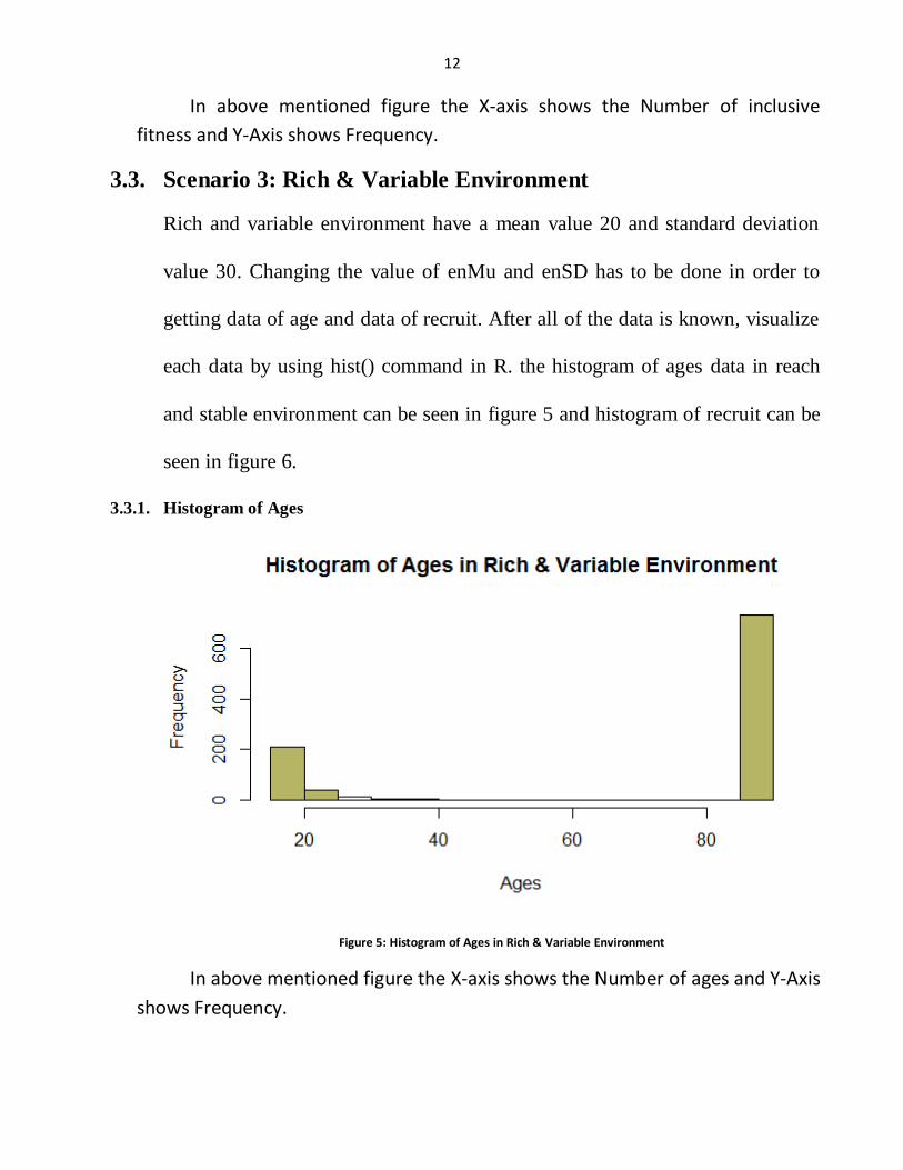
3.3. Scenario 3: Rich & Variable Environment
Rich and variable environment have a mean value 20 and standard deviation
value 30. Changing the value of enMu and enSD has to be done in order to
getting data of age and data of recruit. After all of the data is known, visualize
each data by using hist() command in R. the histogram of ages data in reach
and stable environment can be seen in figure 5 and histogram of recruit can be
seen in figure 6.
3.3.1. Histogram of Ages
Figure 5: Histogram of Ages in Rich & Variable Environment
In above mentioned figure the X-axis shows the Number of ages and Y-Axis
shows Frequency.
13
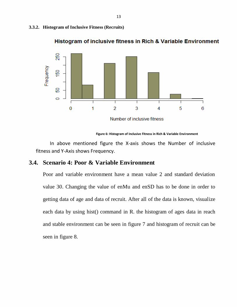
3.3.2. Histogram of Inclusive Fitness (Recruits)
Figure 6: Histogram of Inclusive Fitness in Rich & Variable Environment
In above mentioned figure the X-axis shows the Number of inclusive
fitness and Y-Axis shows Frequency.
3.4. Scenario 4: Poor & Variable Environment
Poor and variable environment have a mean value 2 and standard deviation
value 30. Changing the value of enMu and enSD has to be done in order to
getting data of age and data of recruit. After all of the data is known, visualize
each data by using hist() command in R. the histogram of ages data in reach
and stable environment can be seen in figure 7 and histogram of recruit can be
seen in figure 8.
14
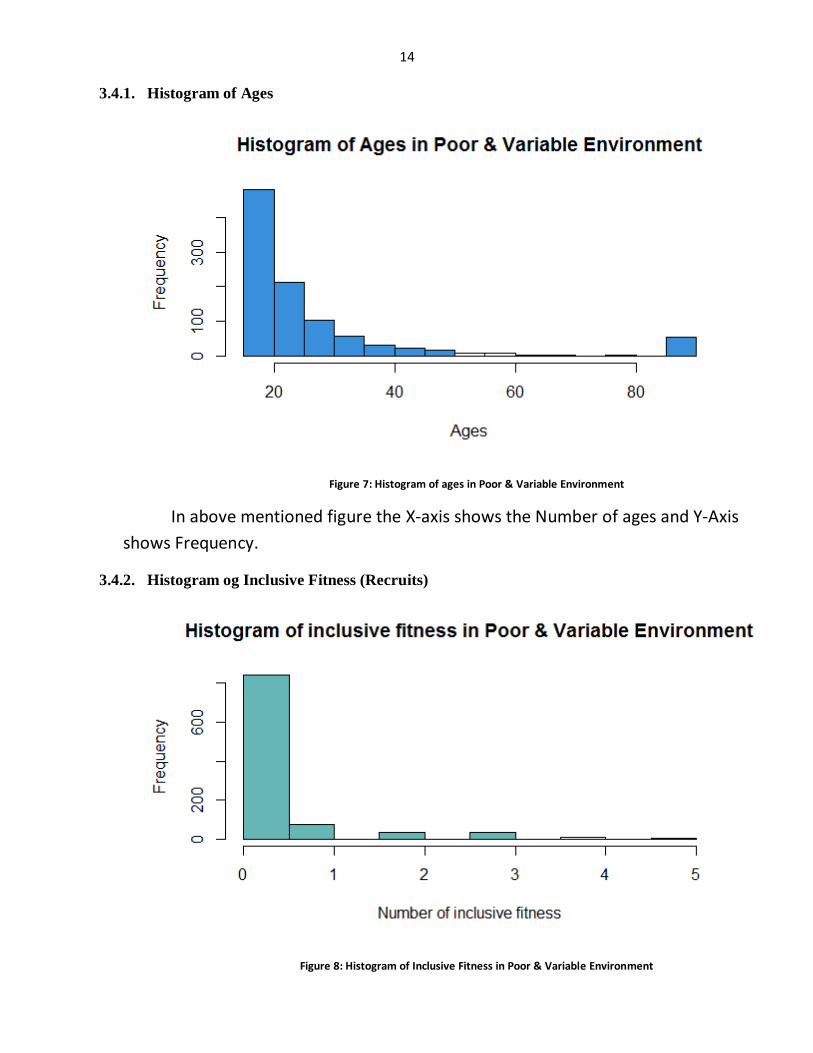
3.4.1. Histogram of Ages
Figure 7: Histogram of ages in Poor & Variable Environment
In above mentioned figure the X-axis shows the Number of ages and Y-Axis
shows Frequency.
3.4.2. Histogram og Inclusive Fitness (Recruits)
Figure 8: Histogram of Inclusive Fitness in Poor & Variable Environment

15
In above mentioned figure the X-axis shows the Number of inclusive
fitness and Y-Axis shows Frequency.
4. Discussion of Results
The purpose of this case study was to observe the effects of quality and
environmental variability on reproductive capacity in female killer whales’
productivity based on age. Following conclusions can be drawn from the analysis:
In rich & stable environment killer-whales have age’s up to 80 years and they
produce offspring maximally up to 3. In poor & stable environment killer wales have
ages less than 20 and they produce offspring 0 out of roundabout 800 whales.
In rich & variable environment killer-whales have age’s more than 80 years and
mostly they produce offspring 0. In poor & variable environment most of the killer
whales have age’s less than 20 and mostly they produce offspring 0.
The maximum of female whales end their reproductively in 80-90 years of old in
rich environment. There is less effect for stable and variable environment on
productivity age. There are a linear decreasing number of whales among one to
three offspring’s they recruits in the age between 15 to 60 years of age.
In case of poor environment maximum number of whales between 14 and 19
years old lose their reproductiveness. Average variable stable environment and has
a certain effect on the poor environment. In stable environment there is an increase
in the number of whales between 20 and 24 who have lost their reproductive
capacity.
16
References
[1] Bradford,A. 2014. Orcas: Facts about Killer Whales. [ONLINE] Available at:
http://www.livescience.com/27431-orcas-killer-whales.html.
[2] http://www.killer-whale.org/killer-whale-information/
[3] http://www.stat.umn.edu/geyer/old/5101/rlook.html
[4] http://statweb.stanford.edu/~naras/jsm/NormalDensity/NormalDensity.html
[5]Assignment given to us (Engr. Ralf Darius)
17
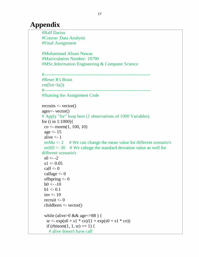
Appendix #Ralf Darius
#Course: Data Analysis #Final Assignment
#Muhammad Ahsan Nawaz #Matriculation Number: 18790
#MSc.Information Engineering & Computer Science
#---------------------------------------------------------------------- #Reset R's Brain
rm(list=ls())
#---------------------------------------------------------------------- #Starting the Assignment Code
recruits <- vector()
ages<- vector() # Apply "for" loop here (1 observations of 1000 Variables)
for (i in 1:1000){
co <- rnorm(1, 100, 10) age <- 15
alive <- 1
enMu <- 2 # We can change the mean value for different scenario's
enSD <- 30 # We cahnge the standard deviation value as well for different scenario's
s0 <- -2
s1 <- 0.05 calf <- 0
calfage <- 0
offspring <- 0
b0 <- -10 b1 <- 0.1
inv <- 10
recruit <- 0
childborn <- vector()
while (alive>0 && age<=88 ) {
sr <- exp(s0 + s1 * co)/(1 + exp(s0 + s1 * co)) if (rbinom(1, 1, sr) == 1) {
# alive doesn't have calf

18
if (calf == 0) {
b <- exp(b0 + b1 * co)/(1 + exp(b0 + b1 * co)) if ((rbinom(1, 1, b) == 1 )&&(age<=40)) {
# give birth
calf <- 1
} } else {
# have calf
co <- co - inv if (rbinom(1, 1, 0.8) == 1) {
# calf alive
calfage <- calfage + 1
if (calfage >= 4) { # independence
offspring <- offspring + 1
childborn <- cbind(childborn,age-5) calf <- 0
calfage <- 0
}
} else { # calf die
calf <- 0
calfage <- 0
} }
age <- age + 1
co <- co + rnorm(1, enMu, enSD) } else {
# female dead
alive <- 0
} }
if (length(childborn)>0){
for (j in 1:length(childborn)){ if ((age-childborn[[j]])>=15&&rbinom(1,1,0.98)==1){
recruit <- recruit + 1
}
}
}
ages <- cbind(ages,age)
19
recruits <- cbind(recruits,recruit)
} hist(ages, main="Histogram of Ages in Poor & Variable Environment",
xlab="Ages", ylab="Frequency" )
#Histograms
hist(recruits, main="Histogram of inclusive fitness in Poor & Variable Environment", xlab="Number of inclusive fitness", ylab="Frequency")