TKK Dissertations in Information and Computer ScienceEspoo 2008 TKK-ICS-D1

DATA ANALYSIS METHODS FOR CELLULARNETWORK PERFORMANCE OPTIMIZATION

Pasi Lehtimaki

Dissertation for the degree of Doctor of Science in Technology to be presented with due

permission of the Faculty of Information and Natural Sciences for public examination

and debate in Auditorium TU2 at Helsinki University of Technology (Espoo, Finland)

on the 3rd of April, 2008, at 12 noon.

Helsinki University of TechnologyFaculty of Information and Natural SciencesDepartment of Information and Computer Science

Teknillinen korkeakouluInformaatio- ja luonnontieteiden tiedekuntaTietojenkasittelytieteen laitos

CORE Metadata, citation and similar papers at core.ac.uk

Provided by Aaltodoc Publication Archive

Distribution:Helsinki University of TechnologyFaculty of Information and Natural SciencesDepartment of Information and Computer ScienceP.O. Box 5400FI-02015 TKKFINLANDURL: http://ics.tkk.fiTel. +358-9-451 3272Fax +358-9-451 3277E-mail: series@ics.tkk.fi

c© Pasi Lehtimaki

ISBN 978-951-22-9282-0 (Print)ISBN 978-951-22-9283-7 (Online)ISSN 1797-5050 (Print)ISSN 1797-5069 (Online)URL: http://lib.tkk.fi/Diss/2008/isbn9789512292837/

Multiprint OyEspoo 2008

Lehtimaki, P. (2008): Data-analysis methods for cellular network perfor-

mance optimization. Doctoral thesis, Helsinki University of Technology, Dis-sertations in Computer and Information Science, TKK-ICS-D1, Espoo, Finland.

Keywords: cellular network, radio network, radio resource optimization, infor-mation visualization, regression, clustering, segmentation, optimization

ABSTRACT

Modern cellular networks including GSM/GPRS and UMTS networks offer fasterand more versatile communication services for the network subscribers. As a result,it becomes more and more challenging for the cellular network operators to enhancethe usage of available radio resources in order to meet the expectations of thecustomers.

Cellular networks collect vast amounts of measurement information that can beused to monitor and analyze the network performance as well as the quality ofservice. In this thesis, the application of various data-analysis methods for theprocessing of the available measurement information is studied in order to providemore efficient methods for performance optimization.

In this thesis, expert-based methods have been presented for the monitoring andanalysis of multivariate cellular network performance data. These methods allowthe analysis of performance bottlenecks having an effect in multiple performanceindicators.

In addition, methods for more advanced failure diagnosis have been presentedaiming in identification of the causes of the performance bottlenecks. This is im-portant in the analysis of failures having effect on multiple performance indicatorsin several network elements.

Finally, the use of measurement information in selection of most useful optimiza-tion action have been studied. In order to obtain good network performanceefficiently, the expected performance of the alternative optimization actions mustbe possible to evaluate. In this thesis, methods to combine measurement infor-mation and application domain models are presented in order to build predictiveregression models that can be used to select the optimization actions providingthe best network performance.

Lehtimaki, P. (2008): Data-analyysimenetelmia matkapuhelinverkkojen

suorituskyvyn optimointiin. Tohtorin vaitoskirja, Teknillinen korkeakoulu, Dis-sertations in Computer and Information Science, TKK-ICS-D1, Espoo, Suomi.

Avainsanat: matkapuhelinverkot, radioverkko, radioresurssien optimointi, in-formaation visualisointi, regressio, klusterointi, segmentointi, optimointi

TIIVISTELMA

Nykyaikaiset matkapuhelinverkot kuten GSM/GPRS ja UMTS tarjoavat yha no-peampia ja monipuolisempia palveluita kayttajilleen. Taman seurauksena verkko-operaattorit joutuvat yha haasteellisempien tehtavien eteen pyrkiessaan tehosta-maan rajallisten radioresurssiensa kayttoa asiakastyytyvaisyyden takaamiseksi.

Matkapuhelinverkot keraavat jatkuvasti runsaasti mittausinformaatiota, jota voi-daan kayttaa verkon suorituskyvyn ja palvelun laadun analysointiin ja paranta-miseen. Tassa vaitoskirjassa tutkitaan erilaisten data-analyysimentelmien sovelta-mista taman mittausinformaation kasittelyyn siten, etta matkapuhelinverkon suo-rituskyvyn analysointi ja palvelun laadun parantaminen tehostuu.

Tassa vaitoskirjassa on kehitetty kayttajakeskeisia menetelmia, jotka mahdollista-vat usean matkapuhelinverkon suorituskykya kuvaavan indikaattorin yhtaaikaisenseurannan ja analysoinnin. Tama mahdollistaa sellaisten suorituskyvyn pullonkau-lojen tunnistamisen, joilla on vaikutuksia useaan suorituskykyindikaattoriin.

Tassa vaitoskirjassa on kehitty menetelmia myos suorituskykyongelmien aiheutta-jien tarkempaan selvittamiseen. Tama on ensisijaisen tarkeaa sellaisten vikatilan-teiden tutkimisessa, joissa suorituskykyongelman aiheuttajalla on suora vaikutususeisiin eri indikaattoreihin ja verkkoelementteihin.

Vaitoskirjan loppuosassa on tutkittu mittausinformaation tehokasta hyodyntamistavarsinaisten optimointitoimenpiteiden valitsemisessa. Jotta parhaaseen suoritus-kykyyn paastaisiin, on vaihtoehtoisten toimenpiteiden vaikutukset suorituskykyynoltava ennakoitavissa. Tassa vaitoskirjassa on esitetty menetelmia, joiden avullaaiemmin kerattya mittausinformaatiota ja sovellusalan teoreettisia malleja voidaankayttaa ennustavien regressiomallien muodostamiseen ja optimaalisten optimoin-titoimenpiteiden valitsemiseen.

Preface

This work has been done in the Laboratory of Computer and Information Sci-ence at the Helsinki University of Technology. I wish to thank my supervisorProf. Olli Simula and my instructor Dr. Kimmo Raivio, for their support duringmy work at the laboratory. Also, I would like to thank Dr. Jaana Laiho, M.ScMikko Kylvaja and M.Sc Kimmo Hatonen at Nokia Corporation as well as Dr.Pekko Vehvilainen and M.Sc Pekka Kumpulainen at Tampere University of Tech-nology for their cooperation during our work with the cellular network performanceanalysis.

I am also grateful to my parents for their continuous support during my studiesat the HUT.

Pasi LehtimakiOtaniemi, March 10, 2008

iii

Contents

Abstract i

Tiivistelma ii

Preface iii

Publications of the Thesis vi

Author’s Contributions vii

Abbreviations x

1 Introduction 1

1.1 Motivation and overview . . . . . . . . . . . . . . . . . . . . . . . . 11.2 Contributions of the thesis . . . . . . . . . . . . . . . . . . . . . . . 11.3 Outline of the thesis . . . . . . . . . . . . . . . . . . . . . . . . . . 2

2 Radio Resource Management in Cellular Networks 3

2.1 Cellular Network Architectures . . . . . . . . . . . . . . . . . . . . 42.1.1 GSM Network . . . . . . . . . . . . . . . . . . . . . . . . . 42.1.2 UMTS Network . . . . . . . . . . . . . . . . . . . . . . . . . 62.1.3 Telecommunications Management Network . . . . . . . . . 6

2.2 Radio Resource Management . . . . . . . . . . . . . . . . . . . . . 82.2.1 Control Loop Hierarchy . . . . . . . . . . . . . . . . . . . . 82.2.2 A Framework for RRM Control Loop . . . . . . . . . . . . 102.2.3 Non-Real Time Performance Optimization . . . . . . . . . . 11

2.3 Cellular Network Performance . . . . . . . . . . . . . . . . . . . . . 132.3.1 Performance Prediction . . . . . . . . . . . . . . . . . . . . 132.3.2 Performance Measurements . . . . . . . . . . . . . . . . . . 15

2.4 Data-Driven Performance Optimization . . . . . . . . . . . . . . . 162.4.1 Expert-Based Approach . . . . . . . . . . . . . . . . . . . . 162.4.2 Adaptive Autotuning Approach . . . . . . . . . . . . . . . . 182.4.3 Measurement-Based Approach . . . . . . . . . . . . . . . . 192.4.4 Predictive Approach . . . . . . . . . . . . . . . . . . . . . . 20

3 Data Analysis Methods 22

3.1 Tasks of Process Monitoring . . . . . . . . . . . . . . . . . . . . . . 223.2 Survey of Research Fields . . . . . . . . . . . . . . . . . . . . . . . 23

3.2.1 Exploring and Visualizing Data . . . . . . . . . . . . . . . . 24

iv

3.2.2 Clustering and Segmentation . . . . . . . . . . . . . . . . . 253.2.3 Classification and Regression . . . . . . . . . . . . . . . . . 263.2.4 Control and Optimization . . . . . . . . . . . . . . . . . . . 27

3.3 Traditional Methods for Regression . . . . . . . . . . . . . . . . . . 283.3.1 Linear Regression . . . . . . . . . . . . . . . . . . . . . . . . 283.3.2 Linear and Quadratic Programming . . . . . . . . . . . . . 29

3.4 Neural Networks . . . . . . . . . . . . . . . . . . . . . . . . . . . . 303.4.1 Neuron Models . . . . . . . . . . . . . . . . . . . . . . . . . 303.4.2 Adaptive Filters . . . . . . . . . . . . . . . . . . . . . . . . 313.4.3 Multilayer Perceptrons . . . . . . . . . . . . . . . . . . . . . 323.4.4 Self-Organizing Map . . . . . . . . . . . . . . . . . . . . . . 33

3.5 Fuzzy Systems . . . . . . . . . . . . . . . . . . . . . . . . . . . . . 353.5.1 Fuzzy Sets, Logical Operations and Inference . . . . . . . . 363.5.2 Fuzzy Inference Systems . . . . . . . . . . . . . . . . . . . . 363.5.3 Adaptive Neuro-Fuzzy Inference System . . . . . . . . . . . 37

3.6 Clustering . . . . . . . . . . . . . . . . . . . . . . . . . . . . . . . . 393.6.1 k-means . . . . . . . . . . . . . . . . . . . . . . . . . . . . . 393.6.2 Davies-Bouldin Index . . . . . . . . . . . . . . . . . . . . . 393.6.3 Cluster Description . . . . . . . . . . . . . . . . . . . . . . . 403.6.4 Clustering of SOM . . . . . . . . . . . . . . . . . . . . . . . 40

3.7 Segmentation . . . . . . . . . . . . . . . . . . . . . . . . . . . . . . 403.7.1 Histogram maps . . . . . . . . . . . . . . . . . . . . . . . . 413.7.2 Operator Maps . . . . . . . . . . . . . . . . . . . . . . . . . 41

3.8 Knowledge Engineering . . . . . . . . . . . . . . . . . . . . . . . . 433.8.1 Variable and Sample Selection . . . . . . . . . . . . . . . . 443.8.2 Constraining Dependencies between Variables . . . . . . . . 453.8.3 Importing Mathematical Models . . . . . . . . . . . . . . . 45

4 Data-Driven Radio Resource Management 46

4.1 Expert-Based UMTS Network Optimization . . . . . . . . . . . . . 464.1.1 Network Scenarios . . . . . . . . . . . . . . . . . . . . . . . 464.1.2 Cell Monitoring . . . . . . . . . . . . . . . . . . . . . . . . . 474.1.3 Cell Grouping . . . . . . . . . . . . . . . . . . . . . . . . . . 52

4.2 Expert-Based GSM Network Optimization . . . . . . . . . . . . . . 534.2.1 A SOM Based Visualization Process . . . . . . . . . . . . . 534.2.2 A Knowledge-Based Visualization Process . . . . . . . . . . 57

4.3 Predictive GSM Network Optimization . . . . . . . . . . . . . . . . 614.3.1 Prediction of Blocking . . . . . . . . . . . . . . . . . . . . . 614.3.2 Prediction of Signal Quality and Dropped Calls . . . . . . . 634.3.3 Optimization of Signal Strength Thresholds . . . . . . . . . 64

5 Conclusions 68

v

Publications of the Thesis

Here is the list of the publications:

1. Pasi Lehtimaki, Kimmo Raivio, and Olli Simula. Mobile Radio Access Net-work Monitoring Using the Self-Organizing Map. In Proceedings of the Eu-ropean Symposium on Artificial Neural Networks (ESANN), pages 231-236,Bruges, April 24-26, 2002.

2. Jaana Laiho, Kimmo Raivio, Pasi Lehtimaki, Kimmo Hatonen, and Olli Sim-ula. Advanced Analysis Methods for 3G Cellular Networks. IEEE Trans-actions on Wireless Communications, Vol. 4, No. 3, pages 930-942, May2005.

3. Pasi Lehtimaki, Kimmo Raivio, and Olli Simula. Self-Organizing OperatorMaps in Complex System Analysis. In Proceedings of the Joint 13th In-ternational Conference on Artificial Neural Networks and 10th InternationalConference on Neural Information Processing (ICANN/ICONIP), pages 622-629, Istanbul, Turkey, June 26-29, 2003.

4. Pasi Lehtimaki and Kimmo Raivio. A SOM Based Approach for Visualiza-tion of GSM Network Performance Data. In Proceedings of the 18th Inter-national Conference on Industrial and Engineering Applications of ArtificialIntelligence and Expert Systems (IEA/AIE), pages 588 - 598, Bari, Italy,June 22-25, 2005.

5. Pasi Lehtimaki and Kimmo Raivio. A Knowledge-Based Model for Ana-lyzing GSM Network Performance. In Proceedings of the 6th InternationalSymposium on Intelligent Data Analysis (IDA), pages 204 - 215, Madrid,Spain, September 8-10, 2005.

6. Pasi Lehtimaki and Kimmo Raivio. Combining Measurement Data andErlang-B Formula for Blocking Prediction in GSM Networks. In Proceed-ings of the 10th Scandinavian Conference on Artificial Intelligence (SCAI),Stockholm, Sverige, May 26-28, 2008 (accepted).

7. Pasi Lehtimaki. A Model for Optimisation of Signal Level Thresholds inGSM Networks. International Journal of Mobile Network Design and Inno-vation (accepted).

vi

Author’s Contributions

Here, the author’s contributions in the publications of this thesis are outlined. InPublication 1, the author developed an extension to the previously existing cellclassification method in order to make it more suitable for cell monitoring purposes,and applied the new method in the analysis of new data set. All computationalwork carried out in Publication 1 was performed by the author.

Publication 2 includes the application of the method presented in Publication1 for a new data set. In Publication 2, the presented method is compared to amore traditional method to analyze cell performance. The author was responsiblefor performing the computational work and interpretation of the results associatedwith the approach presented in Publication 1.

In Publication 3, the cell monitoring approach presented in Publications 1 and 2were modified in order to take the dynamic nature of the data into account whendistinguishing between different states of the cells. The author was responsible fordeveloping the new approach and implementing the software used in the analysis.

Publications 1–3 used only a limited amount of a priori knowledge about theproblem domain. Publication 4 presents a visualization process suitable forthe analysis of the GSM network performance degradations. In this work, priorknowledge about the most common performance degradations is used to focus onthe most interesting parts of the measurement data to be visualized for the user.The author was responsible for developing the method, running all the technicalcomputing and interpreting the results.

In Publication 5, a knowledge-based model is constructed in order to take theprior knowledge into account more efficiently. The available raw data was usedto estimate the free parameters of the knowledge-based model. Finally, the es-timated model is visualized as a hierarchical cause-effect chain representing thedevelopment of the failures in the cellular network. The author was responsiblefor developing the knowledge-based model and estimation of the model parame-ters. The visualization of the cause-effect chains and interpretation of the resultswere carried out by the author.

In Publication 6, the gap between the GSM network measurements and theo-retical calculations associated with cell capacity is discussed. A method that usesboth the Erlang-B formula as well as the network measurements is developed inorder to predict the amount of blocking in SDCCH and TCH channels at differ-

vii

ent amounts of demand. The author was responsible for developing the method,performing all of the computations and analyzing the results.

In Publication 7, the prediction method developed in Publication 6 is appliedin automated parameter optimization. In addition, a model describing the effectsof parameter adjustments to the performance data is defined. The author wasresponsible for developing the model and running the required computations.

viii

ix

Abbreviations

3GPP 3rd Generation Partnership ProjectANFIS Adaptive Neuro-Fuzzy Inference SystemAuC Authentication CentreBMU Best-Matching UnitBR Blocking RateBS Base StationBSC Base Station ControllerBSS Base Station SubsystemBTS Base Transceiver StationCDMA Code Division Multiple AccessCN Core NetworkCSSR Call Setup Success RatioDCR Dropped Call RateFDMA Frequency Division Multiple AccessFER Frame Error RateGPRS General Packet Radio SystemGSM Global System for MobileHLR Home Location RegisterHO HandOverHOSR HandOver Success RatioIMSI International Mobile Subscriber IdentityKPI Key Performance IndicatorLMS Least Mean SquareLU Location UpdateMDS Multidimensional ScalingMLP Multilayer PerceptronMS Mobile StationMSC Mobile Switching CenterNMS Network Management SystemNRM Network Reference ModelNSS Network SubSystemOMC Operation and Maintenance CenterOSS Operations Support SystemPCA Principal Component AnalysisRAA Resource Allocation AlgorithmRNS Radio Network SubsystemRRM Radio Resource ManagementRMSE Root Mean Square Error

x

SDCCH Standalone Dedicated Control CHannelSMS Short Message ServiceSOM Self-Organizing MapTCH Traffic CHannelTCP Transmission Control ProtocolTDMA Time Division Multiple AccessTMF TeleManagement ForumTMN Telecommunications Management NetworkTOM Telecom Operations MapTRX Transceiver/ReceiverUE User EquipmentUMTS Universal Mobile Telecommunications SystemUTRAN Universal Terrestrial Radio Access NetworkVLR Visitor Location RegisterWCDMA Wideband Code Division Multiple Access

xi

xii

Chapter 1

Introduction

1.1 Motivation and overview

The number of mobile network subscribers increases constantly. At the same time,more efficient network technologies are developed in order to provide faster andmore advanced data communication services for the subscribers. As a result, thecurrent and new network technologies operate in parallel, making cost-effectivenetwork management more and more challenging. The network operator shouldbe able to manage the radio resources to meet the current as well as the futuredemand without expensive investments to infrastructure.

This thesis presents approaches in which data-analysis methods, cellular networkmeasurement data and application domain knowledge are combined in order tosolve practical radio resource management problems. In practice, this involves thedevelopment of methods suitable for the detection of abnormal failures and per-formance bottlenecks from multivariate measurement data. In addition to findingbottlenecks in network performance, it is necessary to identify the cause or thelimiting factor for the performance, and to select a management action in order toremove the causes of the failures and performance degradations. The first portionof methods focus on visualization of performance data for human optimizers. Also,methods to predict network performance under different conditions are presented.Finally, an automated method to select the optimal configuration adjustment forthe network is presented.

1.2 Contributions of the thesis

The main contributions of this thesis are:

• the development of data visualization methods for expert-based optimizationof UMTS network plans.

1

• the development of data visualization methods for expert-based optimizationof operative GSM networks,

• the development of knowledge-based predictive models for optimization ofoperative GSM networks.

1.3 Outline of the thesis

The outline of this thesis is as follows. In chapter 2, the problem domain isintroduced in more detail. That is, the GSM and UMTS network architecturesas well as the management of the networks are shortly outlined. The focus ofchapter 2 is on the wide range of methods developed for the optimization of radioresource usage. In chapter 3, the process monitoring problem is discussed, andthe variety of research fields providing tools for process management is shortlyreviewed. The emphasis is on various types of data-analysis methods and theirusage in process monitoring. In chapter 4, the results of applying advanced dataanalysis methods to improve mobile network performance are presented. Finally,in chapter 5, the conclusions are made.

2

Chapter 2

Radio Resource

Management in Cellular

Networks

In this chapter of the thesis, the domain of application, that is, the cellular net-works and their management are discussed. Firstly, the cellular network architec-tures including GSM and UMTS are described. In the following section, a four-layer model for the management of telecommunications networks is described, thefocus being on network management layer of the model.

Then, the focus is turned on the network management functions associated withthe radio network part of the system, and especially, the management of the radioresources. The radio resource management techniques are discussed in severalsections. Firstly, different definitions for radio resource management are given.Then, a framework for using various radio resource management techniques in asystematic performance optimization process is presented.

In the remaining part of this chapter, the non-real time (offline) optimizationloops are discussed. Especially, the focus is on data-driven approaches in whichthe network performance is defined by the BTS level measurements over relativelylong time periods and the optimization is strongly based on intelligent processing ofavailable measurement data collected from the network elements. A comprehensiveliterature study of most widely used approaches for data-driven non-real timeoptimization in both operative GSM networks and UMTS network simulations isconducted.

3

MSC2

AuCVLR

OMC

HLR

OSS

BSC2

MSC1

BTS6

BTS4

NSS

BTS5

CN

BSC1

BSS

BTS3

BTS2

BTS1

BSS

Abis interface

A interface

Figure 2.1: GSM network architecture.

2.1 Cellular Network Architectures

2.1.1 GSM Network

A Global System for Mobile communications (GSM) network consists of Networkand Switching Subsystem (NSS), Base Station Subsystem (BSS) and OperationsSubSystem (OSS). In Figure 2.1, the architecture of GSM network is depicted.

The BSS contains all the radio-related capabilities of the GSM network, beingresponsible for establishing connections between the NSS and the mobile stations(MSs) over the air interface. For this purpose, the BSS consist of several Base Sta-tion Controllers (BSCs) that can manage the operation of several Base TransceiverStations (BTSs) through the Abis interface. Up to three BTSs can be installed onthe same site, and usually, the BTSs are placed to cover separate sectors aroundthe site. Each BTS is responsible for serving the users in its own coverage area,also called the cell, over the air interface. Depending on the user density in thecell served by a BTS, one or more Transceiver/Receiver pairs (TRXs) operatingon separate radio frequencies can be installed to a BTS in order to obtain therequired number of communication channels. In (Kyriazakos and Karetsos, 2004),the architecture of GSM network is described in more detail.

In GSM, the available radio frequency band is divided between different subscribersusing Frequency Division Multiple Access (FDMA) and Time Division MultipleAccess (TDMA) techniques. In practice, this means that up to 8 subscribers mayoperate on a single physical frequency, and the 8 users using the same physicalfrequency are separated by allocating different time slots for each of the users.

On a single physical channel, several logical channels operate in parallel in or-der to establish connections over the air interface. The most important logicalchannels used to implement the basic services such as voice calls, short messageservice (SMS) messages and location updates (LUs) include Standalone Dedicated

4

RNC2

BS6

BS4

BS5

CN

RNC1

RNS

BS3

BS2

BS1

RNS

Iub interface

Iu interface

Iur interface

Figure 2.2: UMTS network architecture.

Control CHannel (SDCCH) and Traffic CHannel (TCH). For example, in voicecall establishment the SDCCH is occupied during the negotiation phase in whichthe actual TCH channel carrying the voice data is allocated. The SMS messagesand the LUs are usually transmitted in SDCCH, but TCH may be used for thatpurpose during congestion situations.

The role of the NSS is to operate as a gateway between the fixed network andthe radio network. It consists of Mobile Switching Centre (MSC), Home Loca-tion Register (HLR), Visitor Location Register (VLR) and Authentication Centre(AuC). The MSC acts as a switching node, being responsible for performing allthe required signaling for establishing, maintaining and releasing the connectionsbetween the fixed network and a mobile user. The Home Location Register (HLR)is a database that includes permanent information of the subscribers. This infor-mation includes International Mobile Subscriber Identity (IMSI) and for example,the identity of the currently serving VLR needed in routing the mobile-terminatedcalls. The VLR contains temporary information concerning the mobile subscribersthat are currently located in the serving area of the MSC, but whose HLR is else-where. The AuC is responsible for authenticating the mobile users that try toconnect to the GSM network. Also, a mechanism used to encrypt all the datatransmitted between the mobile user and the GSM network are provided by theAuC.

The OSS consist of Operation and Maintenance Center (OMC) that is responsiblefor monitoring and controlling the other network elements in order to provideadequate quality of service for the mobile users. In other words, it measures theperformance of the network and manages the network configuration parametersand their adjustments. Therefore, most of the methods and techniques discussedin this thesis are mostly implemented in the OSS.

5

2.1.2 UMTS Network

The Universal Mobile Telecommunications System (UMTS) consist of UniversalTerrestrial Radio Access Network (UTRAN) and the Core Network (CN) con-nected via the Iu interface. In Figure 2.2, the UMTS network architecture isdepicted.

The UTRAN consist of several Radio Network Subsystems (RNSs) that are respon-sible for connecting the User Equipment (UE) to the network. The RNS consist ofRadio Network Controllers (RNCs) and Base Stations (BSs). RNC is the switchingand controlling element of the UTRAN, located between the Iub and Iu interface.The RNC controls the logical resources of its BSs and is responsible, for example,to make handover decisions. The RNC and the BSs are connected through theIub interface, while the RNCs within the same UTRAN are connected via the Iurinterface. For more information about UMTS architecture, see (Kaaranen et al.,2005).

The main tasks of BS include radio signal receiving and transmitting over theUu interface (air interface), signal filtering and amplifying, modulation/spreadingaspects as well as channel coding and functionalities for soft handover. The BSincludes transceiver/receiver equipment to establish radio connections betweenUEs and the network.

In UMTS, the available frequency band is divided between the users on the basis ofWideband Code Division Multiple Access (WCDMA) technique. In (W)CDMA,the data for each user is transmitted in the whole frequency band, and no separa-tion in frequencies nor time is present. Instead, the user data is multiplied by acode sequence unique for each user (code chip-rate is higher than the bit-rate ofthe data). After multiplying the user data with the corresponding codes, a singlespread spectrum signal is obtained and transmitted through the air interface. Atthe receiver, the spread spectrum signal is multiplied by the same, user specificcodes which decodes the original data for each user.

The use of (W)CDMA technique causes the capacity of the UMTS network to bea more difficult issue to handle, and no clear separation between network capacityand coverage can be made. Also, the UMTS radio network becomes interferencelimited rather than frequency limited as is the case with GSM networks.

2.1.3 Telecommunications Management Network

The TeleManagement Forum (TMF) is an international organization consistingof service providers and suppliers from the communications industry. In orderto improve and accelerate the availability of network management products andcompatibility between products from different vendors, the TMF provides highlyauthoritative standards and frameworks for the management of telecommunicationbusiness operations.

The Telecommunications Management Network (TMN) model, as proposed by theTMF, gives a general framework for the processes involved in telecommunication

6

Element Management

Network Management

Service Management

Business Management

Figure 2.3: The TMN model.

business management. The same framework is adopted by 3rd Generation Part-nership Project (3GPP) in order to create a globally applicable 3G generationcellular system known as the UMTS. According to Laiho et al. (2002c), the layersof TMN (see Figure 2.3) consist of

• business management layer,

• service management layer,

• network management layer, and

• element management layer.

The business management layer can be seen as goal setting rather than goal achiev-ing layer, in which high-level planning, budgeting, goal setting, executive decisionsand business-level agreements take place. For this reason, the business manage-ment layer can be seen as strategical and tactical management unit, instead ofoperational management like the other layers of the TMN model. The servicemanagement layer is concerned with tasks including subscriber data management,service and subscriber provisioning, accounting and billing of services as well asdevelopment and monitoring of services. The network management layer managesindividual network elements and coordinates all network activities and supportsthe demands of the service management layer. Network planning, data collectionand data analysis, as well as optimization of network capacity and quality are themain tasks of this layer. The element management layer monitors the functioningof the equipment and collects the raw data.

In addition to the TMN, the TMF has defined a Telecom Operations Map (TOM)in which the processes of the TMN layers are defined in more detail. The TOMlinks each of the high-level processes into a set of component functions and iden-tifies the relationships and information flows between the component functions.

7

The above mentioned frameworks and guidelines help the service providers to de-fine the organization of the human resources and the tasks related to differentparts of the organization. In practice, the tasks adopted from the TOM requirethe use of software tools, which are implemented by the Network ManagementSystems (NMS). The NMS consist of all the necessary tools, applications and de-vices that assist the human network managers to maintain operational networks.The NMS tools are based on open interfaces in order to establish long-term sup-portability for the tools, compatibility between tools from different vendors, butalso to enable rapid development of high quality tools and technologies. For thisreason, the 3GPP has defined a Network Resource Model (NRM). The NRM de-fines object classes, their associations, attributes and operations as well as definesthe object structure which is used in, for example, management of configurationand performance data.

In this thesis, the focus is on the network management layer of the TMN model,and especially, the activities focusing on radio network part of the GSM and UMTSnetworks. This is discussed in the next section.

2.2 Radio Resource Management

2.2.1 Control Loop Hierarchy

The objective of the radio resource management (RRM) is to utilize the limited ra-dio spectrum and radio network infrastructure as efficiently as possible. The RRMinvolves strategies and algorithms for controlling parameters related to transmis-sion power, channel allocation, handover criteria, modulation scheme, error codingscheme, etc. Most of the RRM algorithms operate in a loop, constantly monitoringthe current state of the system, and if necessary, control actions are triggered inorder order to improve radio resource usage.

In (Laiho et al., 2002c), a general hierarchy for different RRM techniques is pre-sented in which the RRM loops are classified into three layers according to theresponse time of the algorithm (length of a single iteration) as well as the amountof information needed by the algorithm (see Figure 2.4). In the bottom layer,the fast real-time RRM loops ensure the adequate quality of the currently activeradio links. These techniques are also called as the resource allocation algorithms(RAA) and examples include serving cell selection and transmission power control.In (Zander, 2001), a wide range of RRM techniques that belong to the fast real-time loops are presented. The fast real-time RRM algorithms for power control,channel allocation and handover control focus on maximizing operators revenue,that is, the incomes of the operator. The maximization of the incomes is closelyconnected with the concept of service quality, since only the services that meetthe quality of service requirements contribute to the income of the operator. Thequality of service are defined for each service, user and link separately, and there-fore the fast real-time RRM loops are designed to meet these quality requirementsfor each link separately. Therefore, the maximization of the incomes implies thatthe number and duration of the communication links filling the quality require-ments must be maximized. The quality of each link is optimized or controlled

8

Planning

Optimization

Fast

Real−Time

Loop

Slow

Real−Time

Loop

Non−

Real Time

Loop

MS

MS

BTS, BS

BTS, BS

BSC, RNC

NMS

NMS

Amount of Information

Res

ponse

Tim

e

Figure 2.4: The hierarchy for RRM control loops.

separately, based on short number of measurements, typically averaged over shorttime intervals. These RRM loops are implemented in the MSs and BTSs.

The middle layer of RRM algorithms consist of slow real-time RRM loops im-plemented in the BSS or RNC of the network. Admission control and handovercontrol algorithms are typically implemented at this layer. The slow real-timecontrol loops perform RRM actions that are needed to maintain link-level perfor-mance, such as triggering a BSC initiated handovers in order to support seamlessmobility. In (Kyriazakos and Karetsos, 2004), a wide range of adaptive dynamicRRM techniques are presented that belong to the second layer of the control layerhierarchy. These are fully automated control methods, but they are more closelyrelated to improving the average performance of the network, that is, their opera-tion affects on all links currently active in the cell. The emphasis in these dynamicreconfiguration methods is in congestion control, that is, making dynamic reconfig-urations to the system when the system becomes highly loaded for relatively shorttime periods. These techniques are usually triggered several times during one day,and the length of congestion period typically lasts no longer than minutes. Exam-ples of such methods for GSM networks include halfrate/fullrate tradeoff, forcedhandovers, dynamic cell resizing and RX-level adjustment.

The top layer of the hierarchy consist of statistical non-real time control loopsimplemented in the NMS. These loops are initiated and iterated offline and theyare used to improve radio resource usage in both operative networks but also innetwork simulations taking place in the network planning phase. In this the-

9

System Under

ControlControl System+

−

Measurement

Output

Disturbance

ErrorTarget Configuration

Figure 2.5: A Framework for control loop design based on control engineering.

sis, the non-real time (offline) control loops based on statistical measurementsare called performance optimization techniques rather than control loops. Theseperformance optimization techniques have the longest response time but more in-formation sources (variables, network elements) than the control loops at the twobottom layers. The aim of these algorithms is to find the optimal configurations(in the long run) without adapting to the natural, daily (short-term) variations inthe traffic patterns. The performance is measured in terms of Key PerformanceIndicators (KPIs) that describe, for example, various failure rates over long timeperiods, and are averaged or summed over all active users. The number of essentialKPIs that need to be analyzed is typically between 10 and 30, and the numberof raw network measurements related to the most important KPIs is hundredsor thousands. For more information about RRM techniques for wireless networkplanning and optimization, see (Laiho et al., 2002c; Kyriazakos and Karetsos, 2004;Lempiainen and Manninen, 2003).

2.2.2 A Framework for RRM Control Loop

In (Halonen et al., 2002), a control engineering framework for RRM control loopsaiming in enhancements in radio system is presented. The aim of the control loopsis to adapt the wireless network configuration parameters so that the performanceof the network is repeatedly improved. In other words, it is a process in which theradio resource management algorithms and techniques are systematically appliedin a loop in order to improve system performance.

In Figure 2.5, a block diagram illustrating the control loop framework is depicted.The control engineering approach regards the

• configuration parameters as system input,

• the user generated traffic is interpreted as unpredictable disturbance for thesystem under control,

• the performance of the network in terms of statistical counters or KPIs isthe output of the system under optimization, and

• the control system is responsible for generating the improved configuration

10

parameters given the deviation between the current performance of the sys-tem and the target performance.

The performance optimization proceeds by measuring the performance of the sys-tem with the current traffic load, and comparing it to the target performance. Theerror or deviation between the current and target performance is fed to the controlmodule, which is responsible for producing a new system configuration in whichthe gap between measured and target performance is decreased. This loop can beiterated until the target performance is met.

Separate optimization loops can be developed for different subsystems of the mo-bile network so that the optimization of the performance of one subsystem has aminimal impact on other subsystems.

In this thesis, the focus is on the top level of RRM methods, that is, on the statisti-cal non-real time performance optimization. Especially, the focus is on data-drivenapproaches for optimization and planning. The control engineering framework isused to distinguish the major functional blocks of the performance optimizationapproaches and to analyze the implementation of the individual blocks and therelationships between the functional blocks. This is important in order to fullyunderstand the benefits of data-driven approaches when implementing RRM con-trol loops based on information extracted from massive data records.

2.2.3 Non-Real Time Performance Optimization

The performance optimization approaches, that is, the statistical non-real timecontrol loops, can be divided into:

• expert-based,

• adaptive autotuning,

• measurement-based, and

• predictive methods.

The most straightforward approach presented in the literature is based on perfor-mance data visualization and active role of human expert in analyzing the data. Inthis expert-based approach, the user is responsible for detecting the performancedegradations from the presented graphical figures. Then, the user should be ableto analyze the cause of the performance degradations. Finally, the user is responsi-ble for deciding the optimal configuration among the alternatives based on his/herunderstanding of the performance bottleneck. In other words, the mapping fromthe alternative configurations to their expected performances takes advantage ofreasoning that need not be represented explicitly as a software algorithm. There-fore, the tasks of the control system are actually performed by human resources.The expert based approach is focused on fault detection and diagnosis and rep-resenting related information in graphical form. The user is then responsible foranalyzing the figures and making the control action decisions.

11

In the adaptive autotuning approach, the performance of the network under thecurrent configuration is measured by collecting data from the output of the sys-tem under control. Then, the control system is responsible for intelligent decision-making in order to update the configuration (parameters) towards better ones.Finally, the new configuration is installed and new performance data is gathered.This loop is repeated until convergence of configuration parameters is obtained.The system under control must be a real operating network or a simulator andthe performance of the current configuration should be possible to measure effi-ciently. The control system is usually equipped with expert-defined control rulesthat aim in selecting improved configuration by exploiting prior knowledge aboutthe performance bottlenecks. The difference between adaptive autotuning andslow real-time control loops like congestion relief algorithms is that the slow real-time control loops are continuously active, and they can be triggered at any time.The adaptive autotuning methods have a clear starting point and duration, andthe configurations achieved during the adaptation are fixed after the adaptationprocess.

The third approach is based on the use of network measurements. The mea-surement data allows the determination of the mapping between the alternativeconfiguration parameters and the system performance explicitly. In this approach,there is no clear feedback from output variables to the updated configuration, butinstead, the improved (optimal) configuration is directly computed from the targetvariables.

The fourth approach is based on developing predictive regression models using pastmeasurements extracted from the network. The estimated models allow the pre-diction of network performance under unseen configurations and therefore, suchmodels are useful in automated performance optimization. In this approach, amodel for the system under control is obtained from past measurement data. Thesystem model enables the computation of the performance with different configu-ration adjustments directly and the system model remains unchanged during theoptimization process. No feedback loop is needed to test configurations during thedecision making about the new configuration.

It should be mentioned here, that some of the autotuning methods developed forperformance optimization can be implemented as fully automated slow real-timeloops. Also, some of the autotuning methods developed for planning purposesmay be directly applied in optimization of operational networks as a non-real timecontrol loop or a slow real-time loop.

In the following sections, examples of above mentioned approaches for parameteroptimization in operative GSM networks and UMTS network simulations per-formed during network planning are presented. In particular, the focus is ondata-driven techniques in which real or simulated network data is used as a sourceof information in decision making regarding the optimal control action.

12

2.3 Cellular Network Performance

In cellular network planning phase, for example, no performance measurementslike KPIs from live network are available and therefore, predictions of perfor-mance must be used in decision making. Also, early testing of new optimizationalgorithms in operative cellular networks may not be desirable in order to avoidunnecessary risks of confusing the current network configuration. For these rea-sons, most of the algorithms and methods developed for optimization of GSM andUMTS network performance are developed and tested with network simulators.From the optimization algorithm point of view, there is no significant differencein whether the performance of live network or simulated network is optimized.Therefore, it is possible to use most of the presented methods in both optimiza-tion of live network, but also in final phases of the network planning process whichis strongly based on simulators. Firstly in this section, some basic theoretical mod-els used for network performance predictions are reviewed. Then, the performancemeasurements of a real mobile network are introduced. Finally in Section 2.4, theperformance optimization approaches presented in the literature are outlined.

2.3.1 Performance Prediction

Path Loss Models

The most frequently used models associated with network planning and simulationinclude various path loss models. The purpose of the path loss models is to computethe amount of attenuation in the radio signal on the propagation path. A modelbased on pure theoretical derivations is the ideal path loss model where link gainG(R) at distance R is defined by

G(R) =C

Rα(2.1)

where C is an antenna parameter and α is a parameter describing the propagationenvironment (Zander, 2001). In decibel scale, the amount of path loss at distanceR is

L(R) = 10 log G(R) = 10 log C − 10α log R. (2.2)

The value α = 2 is used for free space and values from 3 to 4 are used in urbanenvironments.

Another widely used path loss model for the urban environments is the Okumura-Hata model

L(R) = 26.16 log f + (44.9− 6.55 log hBTS) log R

−13.85 log hBTS − a(hMS) + 69.55, (2.3)

where f is the carrier frequency, R is the distance between BTS and MS antennas,hBTS is the height of the BTS antenna and hMS is the height of the MS an-tenna (Hata, 1980). The function a(hMS) can be selected from three alternativesdepending on the carrier frequency and the type of the operating environment(large, medium or small city).

13

The above mentioned path loss models are used, for example, in initial networkplanning phase (dimensioning) in order to compute the maximum operating rangeof 3G network base stations for given maximum transmission powers (Holma andToskala, 2004). In addition, path loss models are used to predict the relationshipbetween the original signal and interference, having direct impact on signal qualityin the radio links.

Capacity of GSM network

One of the most important performance criteria in mobile networks is the avail-ability of resources (communication channels) with variating traffic load. In orderto predict the amount of traffic that can be supported, the blocking probability iscalculated. Traditionally, the Erlang-B formula is used as a model when computingthe amount of blocking with different number of channels and demand (Cooper,1981). For example, consider the case when the incoming transactions follow thePoisson arrival process with arrival rate λ, transaction length is exponentially dis-tributed with mean 1/µ and the number of channels Nc is finite. The probabilitythat n channels are busy at random point of time can be computed using theErlang-distribution

p(n|λ, µ,Nc) =(λ/µ)n/n!

∑Nc

k=0(λ/µ)k/k!. (2.4)

Using this formula, it is possible to calculate the amount of traffic that is supportedwith given blocking probability. If the Erlang-B formula is applied in networkplanning (dimensioning), the number of communication channels that are neededis computed in order to meet the traffic and blocking probability requirements.

Capacity of UMTS network

Since the UMTS network supports several bit-rates and the capacity in networksusing WCDMA multiplexing is interference limited, the estimation of the capacityis based on calculations in which the transmission powers and path losses for eachactive radio link must be known. The capacity of a WCDMA base station ismeasured, for example, in terms of uplink loading

ηul = (1 + i)

N∑

j=1

1

1 + W/ [(Eb/N0)jRjvj ](2.5)

where (Eb/N0)j is the signal to interference ratio of radio signal for user j, W isthe chip-rate, Rj is the bit-rate of user j and vj is the activity of the user j. Itshould be noted here, that the consumption of wireless network resources causedby a single user depends on the bit-rate of the service used, the speed of the user,and the path loss (distance) influencing the radio signal. Also, the number of usersin the adjacent cells affect on cell capacity due to the interference originating fromthe surrounding cells. The higher the bit-rate of the used service, the greater theload factor for single user becomes. The larger the load factors of individual activeusers are, the less new users can be allocated to the system.

14

This load factor can be directly used to estimate the amount of interference (noiserise) in addition to the basic noise floor caused by thermal noise.

In networks based on WCDMA , the estimation of the blocking probability musttake the occurrences of soft handover into account. The so-called soft capacityindicates the amount of traffic that can be supported by a WCDMA cell withprespecified blocking probability. A computational procedure for evaluating thesoft capacity based on Erlang-B formula is described in (Holma and Toskala, 2004).

2.3.2 Performance Measurements

The operation of the cellular network can be interpreted to consist of a sequenceof events. From the network operation point of view, certain events are closelyassociated with bad performance, lack of resources or failures. The number ofundesired events during a measurement period (typically one hour) are storedby a set of corresponding counters. In this thesis, the performance of operativecellular networks is determined by the number of undesired events, such as blockedchannel requests and dropped calls. The optimization of operative networks aimsin minimizing the number of occurrences of such events.

Since the raw data consisting of the values of the counters at different time periodsis impractical to analyze as such, a wide range of KPIs are defined that aim in moreintuitive performance analysis (Halonen et al., 2002; Kyriazakos and Karetsos,2004). The most important KPIs include the SDCCH and TCH Blocking Rates(SDCCH/TCH BR), Dropped Call Rate (DCR), Call Setup Success Rate (CSSR)and Handover Success Rate (HOSR). These KPIs can be computed in differentways depending on the network vendor and the operator, but in general, they arecomputed by dividing the number of undesired events with the total number ofattempts. For example, the DCR can be computed by dividing the number ofdropped calls due to inadequate radio link quality and other similar reasons in ameasurement period with the total number of calls in the measurement period.

However, the KPIs are mostly useful in fault detection rather than studying theactual cause of undesired events. For example, the dropped calls can be causedby failures in the A, Abis or air interfaces or any other related network element.Observing a certain value of DCR does not indicate which of the network elementof interface caused the calls to be dropped. In order to isolate the cause, thecounter data must be studied. However, the use of counter data not always givesthe actual cause for the undesired events. For example, the cause for bad radio linkquality can be shadow fading or multipath fading, but also, interference originatingfrom other cells operating on the same frequency has an effect on signal quality.There are no measurements available that could be used to distinguish betweenthese different causes for bad signal quality.

Another difficulty with the use of KPIs in performance analysis is caused by stronginteractions between close-by BTSs. For example, the HOSR can be on unaccept-able level, but further analysis might reveal that the problem occurs mostly duringthe outgoing handovers into a certain close-by BTS. A possible explanation forfailed incoming HOs may rely in lack of TCHs in the target cell. Therefore, the

15

capacity problems in a close-by BTS may be visible in HOSR of a BTS, and itis necessary to simultaneously analyze several KPIs from close-by BTSs in orderto fully recognize the location of the bottleneck in network performance. Similardependencies between KPIs may exist between BTSs on the same physical carrier,or between the BTSs sharing some other physical resources.

2.4 Data-Driven Performance Optimization

2.4.1 Expert-Based Approach

In the literature, a wide range of radio network optimization methods exploitingvisualization and expert decision making are proposed. The expert-based ap-proach has been studied using performance data from network simulators and livenetworks.

In (Zhu et al., 2002), a set of indicators are proposed for the detection of over-loaded cells. The method is used to optimize pilot power settings in an UMTSnetwork in order to obtain better network performance. A dynamic network sim-ulator is used to demonstrate the benefits of the proposed indicators. The abovemethod is based on designing good indicators that can be visualized in very simpleform, such as time-series data or histogram. However, the visualization of perfor-mance data of a wireless network has been tackled also with advanced data analysismethods such as neural networks. For example, the works by Raivio et al. (2001)and Raivio et al. (2003) demonstrate the use of clustering and neural networksin the visualization of operational states computed from multivariate uplink per-formance data of a WCDMA network. Also, the problem of finding similar basestations according to uplink performance is tackled, enabling the simplification ofautotuning of key configuration parameters.

The work presented in Publication 1 is a modification to the above mentionedmethod. In Publication 1, the downlink performance degradations in WCDMAnetwork simulation are detected during continuous monitoring of the state of thenetwork. The current states of the BSs are classified according to the shape of thedistribution of the related performance variables over short time periods. The end-user is provided a simplified description of the possible states of the BSs. Then, theuser is able to find out which of the obtained states are inappropriate for the BSs.By using a digital map roughly describing the radio signal propagation conditionsin the network area, the end-user is responsible for deciding what is the limitingfactor for the network performance. Also, the end-user is responsible for decidinghow the configuration should be adjusted in order obtain better performance forthe planned network.

In Publication 2, the same methodology has been applied for the analysis of up-link performance of a microcellular network scenario and comparisons to perfor-mance analysis based on WCDMA loading equations are presented. The presentedmethod can also be used in cell grouping, aiming in more efficient optimizationof large amount of BSs since similar BSs may share the same configuration pa-rameters. In (Laiho et al., 2002b), the same methodology has been applied for

16

the analysis of uplink performance in a microcellular network scenario, but also,the flexibility of the presented methodology is demonstrated by using the samemethod in the analysis of uplink and downlink performance simultaneously bothin micro- and macrocellular network scenarios. The general use of cell grouping inthe network optimization process is discussed in (Laiho et al., 2002a) and (Laihoet al., 2002b).

In Publication 3, the problem of continuously monitoring the states of the cellsis approached from a new perspective. The definition of the BS state used inperformance monitoring and state classification is based on dynamics of the linkperformance. A linguistic description of the dynamics of the alternative BS statesis provided. Using them, the user is responsible for deciding which states areinappropriate and how the BSs in such states should be adjusted.

Vehvilainen (2004) and Vehvilainen et al. (2003) give a comprehensive study forexploiting data mining and knowledge discovery methods in performance analysisof operative GSM networks. The use of soft computing techniques like rough sets,classification trees and Self-Organizing Maps for the easy analysis of importantfeatures of the performance data is discussed. In addition, methods to use a prioriknowledge, that is, the application domain experience in the analysis process isgreatly emphasized.

In (Multanen et al., 2006), a method to use KPI data from live GSM networkto find city-sized low performing subnetworks from a very large network areasis presented. This method applies well for determining locations of performancedegradations in which optimization should take place.

In Publications 4-5, the analysis of performance degradations in city-sized GSMnetworks is studied. In Publication 4, a method to analyze the real KPI dataof an operating GSM network with neural network based visualization process isdescribed. Several different kinds of visualizations are provided in order to helpuser’s task to analyze alternative causes for the performance degradations. Theuser is responsible for deciding how the configuration should be adjusted in orderto prevent the same performance degradations to appear in the future. The mainbenefit of this approach is that the same methods can be applied in optimizationof many different configuration parameters and network subsystems with low costsas long as required expertise is at hand. For example, in Publication 4, the samemethod is used to analyze TCH and SDCCH capacity problems without any majormodifications to the method. Also, the same methods are available for the analysisof operative networks as well as for the analysis of simulated data being the outputof, for example, network planning activities.

However, the use of the expert-based methods requires extensive knowledge aboutthe problem domain and the optimization actions proposed by different expertsmay not be consistent. Also, the main disadvantages of these methods includethe inability to observe how close-by cells interact during faulty situations. Fur-thermore, the visual analysis of KPI data may be misleading, since the averagingperformed during KPI computation lose essential information about the true sourceof the performance degradation.

In order to cope with these difficulties, a data-driven approache using the counter

17

data instead of KPI data may be used. In Publication 5, an explicit descriptionof the network performance development is presented in order to study the cause-effect chains in which the bad performance is developing. Possible cause-effectrelationships between the most important counters are searched from the dataand presented for the end user in a tree-structured cause-effect chains. Also, themain objective was to study the bad performance situations in which the cause isin fact located in close-by BTSs.

Ricciato et al. (2005) have presented methods to discover bottlenecks in perfor-mance of live UMTS network. Several indicators of bottlenecks in TCP (Transmis-sion Control Protocol) packet data transmissions are proposed. The visualizationused in this work is based on plotting the proposed indicators in the form of time-series in which the presence of the bottlenecks are easily captured.

2.4.2 Adaptive Autotuning Approach

One of the most widely adopted approaches for performance optimization is theadaptive autotuning approach in which the initial configuration parameter valuesare repeatedly updated with better ones until convergence is obtained. The meth-ods following this approach repeatedly change the configuration and measure theimprovement in real network or apply a network simulator.

In (Olofsson et al., 1996) and (Magnusson and Olofsson, 1997), the design ofoptimal neighbor lists used by handover algorithms in GSM networks is discussed.The aim was to design an automatic procedure in order to avoid manual adjustmentof neighbor lists for each cell. The presented method was based on simulationsin which the potential new neighborhood relations were tested, and if the newrelation proved out to be useful in the long run, it was finally included in theupdated cell list.

Barco et al. (2001) have studied the optimization of frequency plans based oninterference matrices. The interference matrices are derived from the measurementreports sent by the mobiles. The presented technique is tested under GSM/GPRSsimulator, but it is mentioned, that field trials have provided good results alsounder live network environments.

For the performance optimization of UMTS networks, very similar approaches havebeen presented. Especially, the use of heuristic rules for deriving the improved con-figuration has been proposed frequently. Nearly all of the optimization techniquesare developed under simulator based experiments. For example, Valkealahti et al.(2002b) suggest a rule-based control strategy in order to optimize common pilotpower settings in an UMTS network. The work by Love et al. (1999) also proposesa rule-based approach for the optimization of pilot powers in a CDMA cellularsystem. In (Hoglund and Valkealahti, 2002), a similar method has been presentedfor the optimization of downlink load level target and downlink power maxima. In(Hoglund et al., 2003), the uplink load level target has been optimized with simi-lar, rule-based approach. In (Valkealahti and Hoglund, 2003), several parametersare optimized simultaneously with similar approach.

Another strategy in the autotuning approach is based on minimization of formally

18

defined cost functions rather than the use of heuristic control rules. The optimiza-tion of common pilot power by minimization of the formal cost function with agradient method has been proposed in (Valkealahti et al., 2002a). In (Flanaganand Novosad, 2002a) and (Flanagan and Novosad, 2002b), a technique for findingsoft handover parameters that provide minimal blocking in the network have beenpresented. Flanagan and Novosad (2003) suggest a cost function based approachfor optimization of multiple parameters simultaneously, including soft handoverparameters, uplink and downlink power maxima, as well as uplink and downlinkload targets. Hamalainen et al. (2002) have presented a cost function based au-totuning method for the determination of planned, service specific Eb/No targets.Zhu and Buot (2004) discuss the dependencies between different KPIs and theirsensitivities with respect to the optimized parameters. A sensitivity matrix is com-puted and the autotuning approach is based on the computed sensitivity matrix.Even tough the above mentioned approaches for UMTS network optimization areall tested with radio network simulators, they can be used also to optimize oper-ating WCDMA networks without any major modifications to the control actiondecision making.

The adaptive autotuning approach has been applied in optimization of live GSMnetwork by Magnusson and Oom (2002). The signal strength thresholds used incell selection strongly affects the size of the cells, and therefore, they are tuned inorder to obtain an optimal traffic balancing between cell layers. Simple intuitiverules are used to decide how the current configuration should be adjusted basedon the performance measurements.

Toril et al. (2003) have proposed an algorithm for automatic offline optimizationof handover margins in a live GSM network. The presented method is basedon updating the current handover margin with a simple heuristic update ruledepending on current amount of traffic and blocking.

The main characteristic of the above mentioned methods is that the mapping fromthe alternative configuration settings to the performance of the different configu-rations is determined by testing each of the configurations for certain amount oftime in the live network or simulator. Human-defined heuristics or gradients ofthe objective function are used to select the direction and magnitude of the searchin an intelligent manner in order to obtain faster convergence. Still, testing a largenumber of feasible configurations is a very time-consuming task and therefore,optimization of large number of network elements and parameters simultaneouslymay not be practical. For this purpose, the base stations could share the sameoptimized value of the parameters or they could be assigned into groups of similarBSs, and the BSs in the same group could use the same parameter values, thusdecreasing the dimension of the parameter space. In Publications 1-3, possiblemethods to obtain this cell grouping have been presented.

2.4.3 Measurement-Based Approach

The third approach for the non-real time performance optimization is based on theuse of network measurements directly in decision making. That is, the availabledata can be directly used to construct the configuration to performance mapping

19

without the need of advanced data-driven inference. In (Toril et al., 2002), level-quality data generated by a GSM/GPRS network simulator was gathered, and amapping between the received signal strength and the network performance wasobtained. Then, the selection of the updated signal level threshold was based onoperator requirements for the signal quality with certain confidence level.

In (Chandra et al., 1997), handover related parameters were selected based onsimilar data records. During the operation, the network produced a data set thatallowed the construction of mapping between the handover parameters and theamount of traffic carried by the cell. Nonlinear optimization was used to find theoptimal parameter value given the previously mentioned mapping.

In both of these studies, the used measurement data allowed the determination ofthe mapping between the alternative configuration parameters and the system per-formance explicitly. The drawback of this approach is that reliable measurementdata allowing the determination of the mapping between the configuration and thesystem performance is not available for most of the essential network parameters.

2.4.4 Predictive Approach

Once the bottlenecks of the performance are found, it is necessary to adjust theconfiguration in order to maximize the performance according to the operatorsneeds. In the previous section, different approaches to decide the optimal controlaction were discussed. However, the decision about the new configuration may bevery difficult to make without knowledge of how the network will behave in thenew, unseen configuration. Predictive models can be applied in order to help andto automate the decision-making procedure.

In the study by Steuer and Jobmann (2002), traffic balancing through optimiza-tion of cell sizes is discussed. The cell sizes were modified by adjusting the signalstrength thresholds, handover hysteresis settings and sector shapes of the smartantennas in order to avoid blocking. The presented approach is based on measure-ments including the locations of the mobiles. The method makes predictions aboutthe performance of the system with the new, unseen configurations that are usedto select the optimum setting, therefore being based on predictive modeling. Theavailable data including the mobile locations were the driving force for decidingthe optimal traffic balancing. The benefits of this study were demonstrated withGSM simulations.

The use of predictive modeling approach requires the use of common applicationdomain models in order to make the necessary predictions about the performanceof the adjusted configuration. However, the theoretical predictions and observa-tions made from a real network are not always directly similar or comparable. InPublication 6, the significant differences between theoretical predictions and truemeasurements are highlighted. Also, a method to combine the use of common the-ories and measurement data in order to provide more accurate predictions aboutblocking in GSM networks is presented.

In Publication 7, a predictive modeling based approach is proposed for the op-timization of signal strength thresholds in operative GSM networks. The model

20

includes a data-driven component exploiting the past measurements for the deter-mination of the mapping between current configuration parameters and networkperformance and a knowledge-based component based on common theoretical mod-els allowing the prediction of network performance under unseen configurations.These results are strongly based on the results provided in Publication 6.

21

Chapter 3

Data Analysis Methods

In this chapter, the data analysis methods used in this thesis are described. Firstly,the process monitoring tasks in data-rich production or manufacturing processesare discussed. Then, a wide range of methods and their usage to solve processmonitoring tasks are described.

3.1 Tasks of Process Monitoring

In the process and manufacturing industries, there is a strong tendency to produceend-products of higher quality, to satisfy environmental and safety regulations andto reduce manufacturing costs. In mobile communication industry, there is a pushto provide mobile communication services meeting the quality of service agree-ments for constantly increasing number of subscribers. However, the improvementof the product manufacturing or service provision is complicated by faults occur-ring in the processes. According to Chiang et al. (2001), “a fault is defined asan unpermitted deviation of at least one characteristic property or variable of thesystem” and in order to satisfy the performance requirements, the faults need tobe

• detected,

• identified,

• diagnosed, and

• removed.

These tasks can be tackled by process monitoring methods. Fault detection isdefined as determination of whether a fault has occurred or not. Fault identificationinvolves selection of variables most relevant for the diagnosis of the fault. In faultdiagnosis, the actual cause of the fault, but also, the type, location, magnitude, andtime of the fault are determined. Process recovery involves removing the effects ofthe fault.

22

3.2 Survey of Research Fields

In engineering literature, a wide range of computational, data-driven methods thatcan be efficiently used in different process monitoring tasks have been presented. Itturns out that methods useful for various process monitoring tasks are developedunder very different research fields.

In traditional statistics, data analysis focuses on careful experiment design, hy-pothesis definition, data gathering and hypothesis testing. The emphasis is onconfirmatory data analysis, that is, hypotheses about phenomena are made, andstatistical tests are used to reject or confirm the hypotheses. For more informationabout statistical hypothesis testing, see (Meyer, 1975) and (Milton and Arnold,1995). The tests usually involve estimation of models, for example, linear regres-sion models and testing the significance of the dependency. Also, a wide range ofmathematical tools like sample mean, variance and median are available to sum-marize the information of experimental data. In addition, horizontal bar charts,pie charts, line charts and scatter plots are often used to depict information aboutone variable, to hunt for correlations between variables and to graph multivariatedata. The traditional statistical techniques are frequently used in quality con-trol of industrial systems. For more information about traditional quality control,see (Mitra, 1998) and (Chiang et al., 2001).

Due to the rapid development of computer aided systems, the amount of availabledata has truly exploded and traditional hypothesis testing is no longer an efficientapproach for many cases. One of the most recent and rapidly growing researchfields related to inference in data-rich environments is data mining. According toHand et al. (2001), “data mining is the analysis of (often large) observational datasets to find unsuspected relationships and to summarize the data in novel waysthat are both understandable and useful for the data owner”. In other words,data mining focuses on methods that can be used to rapidly increase the amountof knowledge of a system from which data is available. The emphasis is on hy-pothesis generation rather than testing well defined hypothesis. The main tasksof data mining include exploratory data analysis, descriptive modeling, predictivemodeling, pattern and rule discovery and retrieval by content. For the analysisof unknown systems, the explorative data analysis task is the most important onein order to find out the basic structure of the data, see Hoaglin et al. (2000).Another useful set of methods developed under data mining discipline focus on de-scriptive modeling, in which structure in (multivariate) data is typically searched.Descriptive modeling consists of clustering and segmentation methods that applywell for fault detection problems in many industrial applications. The data miningmethods for predictive modeling typically consists of classification and regressiontechniques. They are most useful in fault detection, identification and diagnosisof faults.

The science of graphical representation of data sets is also studied by an ownresearch field, data visualization, that is strongly rooted in the exploratory dataanalysis. However, it has similar aims as statistics and basic scientific visualiza-tions. According to Spence (2007), visualization means “forming a mental modelor mental image of something”. Another frequently quoted justification for datavisualization states that “solving a problem simply means representing it so as

23

to make the solution transparent”. Advanced visualization techniques have beendeveloped due to the rapid increase in amount of data to be represented. Mod-ern visualization techniques often rely on projection methods, in which the datais first projected into lower dimension, and the projected data is visualized withbasic graphs. Therefore, the method for summarizing or data reduction differfrom more traditional statistics. Visualization can be effectively used in differentprocess monitoring tasks.

In artificial intelligence, the aim is to create machines to automate tasks requir-ing intelligent behavior. Machine learning is a subfield of artificial intelligencethat concerns algorithms and methods that allow computers to learn from ex-amples. For this reason, machine learning techniques are frequently applied intasks in which process data are used to learn useful relationships in the process.The learning problems are typically very closely related to clustering, regressionand classification methods (Cherkassky and Mulier, 1998). However, the focusof machine learning is on the computational properties of the methods such ascomputational complexity.

A sub-field of machine learning more focused on practical applications of learningmethods is pattern recognition. It includes a wide range of information processingproblems of great practical importance. For example, speech recognition, classifica-tion of handwritten characters, fault detection in machinery and medical diagnosisare important topics in pattern recognition (Bishop, 1995). Most of the recogni-tion problems take the form of clustering, regression or classification, preceededby careful data preprocessing and feature extraction.

System control is a field of engineering in which the aim is the control the operationof a system so that it would function as intended, for example, in a productionprocess (see Astrom and Wittenmark (1997)). The focus is not in management ofunsuspected faults, but instead, the maintenance and optimization of the normaloperational modes. An important part of system control is the system identifica-tion step, in which a mathematical model for system behavior is estimated frommeasurement data. System identification techniques are outlined in (Ljung andGlad, 1994). The system identification consists of similar methods and proceduresas the predictive modeling techniques studied in the data mining, pattern recog-nition and machine learning communities. However, the identification of systemsaiming in system control typically involves estimation of dynamical models fromthe data.

Next, the basics of above approaches and how they can be used in different processmonitoring procedures are discussed. Then, different techniques such as neuralnetworks, fuzzy systems etc. are described and how they can be used in abovementioned process monitoring problems.

3.2.1 Exploring and Visualizing Data

In (Hoaglin et al., 2000), a wide range of tools for explorative data analysis aredescribed. The most simple examples of such tools include stem-and-leaf plots,letter-value displays and N-number summaries. In these techniques, the experi-

24

mental data or a batch is presented by a set of numbers describing the locationand spread of the observations.

Hand et al. (2001), Fayyad et al. (2002) and Spence (2007) give a good summaryof basic tools to visualize univariate and bivariate data. Univariate data is oftendisplayed as histogram or box plots, and bivariate data is typically displayed asscatterplots. If the second variable is time, a time-series plot is often used.

The visualization of multivariate data can be done in at least two ways. Themultivariate data can be visualized with, for example, Chernoff’s faces (Chernoff,1973) or parallel coordinate techniques (Inselberg and Dimsdale, 1990). Also,projecting the data into two dimensions and the use of basic bivariate data plotsis of common practice. The projection is typically based on Principal ComponentAnalysis (PCA) (Hotelling, 1933), Multidimensional Scaling (MDS) (Torgerson,1952; Young, 1985) or Self-Organizing Maps (SOM) (Kohonen, 2001).

By using exploratory data analysis and data visualization techniques, a human an-alyst can efficiently study the information content of the data, and then, importantconclusions and problem refinement emerge. For example, the analyst may be ableto find out what are the most typical failure types of the processes, and it helpsthe researchers to focus on certain subproblems more closely related to the faultof interest. These methods are useful especially in fault detection applications inwhich all the possible fault types are not known in advance, but instead, new typesof faults may occur. In this kind of applications, previously defined fault types anddetection based on them do not necessarily provide adequate solutions. This isthe case in mobile communication networks in particular, since new hardware andradio resource algorithms may be installed and integrated to the existing system,and the compatibility between different algorithms and equipment and possibleside effects are not necessarily known.

3.2.2 Clustering and Segmentation

Another useful data analysis problem type is clustering. In clustering, the datais separated into groups or clusters so that the similarity between samples in thesame cluster is maximized and the similarity between samples in different clustersis minimized.

According to Hand et al. (2001), clustering algorithms can be divided into threeclasses: those based on finding the optimal partitioning of the data into a speci-fied number of clusters, those aiming in finding the hierarchical structure of thedata, and those based on probabilistic models searching for the underlying clusterstructure. The clustering algorithms aiming in dividing the data into specifiednumber of clusters are referred as partitive algorithms. The hierarchical clusteringalgorithms that search for the structure of the data can be divided into top-down(divisive) and bottom-up (agglomerative) algorithms. For more information aboutalgorithms, see Everitt (1993).

As the definition of clustering implies, the characterization of distances betweensamples and clusters is of great importance in clustering of data. For example,the selection of the measure for the within-cluster and between-clusters distances

25

greatly influences the solution returned by the algorithm. The within-cluster andbetween-clusters distances can be measured in several ways. For example, thewithin-cluster distance can be evaluated with average distance between each sam-ple pair in the same cluster, or with the average distance of each sample fromthe centroid of the cluster. The between-clusters distances can be based on forexample, the distances between the cluster centroids.

One of the main problems in data clustering is the availability of wide rangeof algorithms that tend to search for very different types of clusters from thedata. Even the use of same clustering method with different number of targetclusters raises the question of which clustering serves the problem solving processadequately. In the literature, several clustering validity indices have been proposedin order to select the optimal clustering, for more information, see Bezdek and Pal(1998).

A data analysis problem closely related to clustering is the segmentation of time-series data. In time-series segmentation, a sequence of N consecutive (multivariate)data samples is partitioned into groups so that each segment is as homogenousas possible (Bellman, 1961; Terzi, 2006). The homogeneity can be defined inseveral ways. Typically, each segment is represented by a model, for example, adistribution or a time-series model. Similarly to the clustering algorithms, top-down and bottom-up approaches for time-series segmentation have been proposed.A good review of segmentation approaches have been presented in (Terzi, 2006).

Clustering and segmentation techniques are useful in fault identification and di-agnosis. For example, clustering can be used to divide the process data into adiscrete set of states, and some of the states may represent undesired process con-ditions. By studying the properties of such clusters, the causes of the faults maybe analyzed. In addition, the properties of the found fault clusters can be storedand used later in fault detection. The segmentation algorithms can be used insimilar fashion. Especially, when the changes of the states occur more slowly thanthe sampling rate of the measurements, it is more natural to apply segmentationalgorithms than clustering of rapidly changing data samples. In addition, seg-mentation can be used for separating between different operational modes of theprocess.

3.2.3 Classification and Regression

Classification and regression belong to the so-called supervised learning tasks. Inclassification, each sample x is assigned to one of the several classes C. The goalis to find a classification function C = f(x) that is able to predict the classes ofunseen samples x with minimal classification error. The classification function isestimated from labeled data, that is, using a data set consisting of N examplesof (xi, Ci) pairs, i = 1, 2, . . . , N . In regression, the model output is continuousand may consist of several variables. In other words, the learning task consist ofestimating a regression function y = f(x) using examples of xi and yi in order topredict new samples with minimal prediction error.

For classification and regression, a wide range of methods is available. In (Milton

26

and Arnold, 1995) and (Jørgensen, 1993), the basic linear regression for singleand multivariate cases are described. The principles of linear regression modelscan also be extended to fit to many nonlinear modeling problems. In (McCullaghand Nelder, 1983), a wide range of such extensions are described. One of themost interesting approach is based on estimating black-box models using neuralnetworks. The neural network based classification and regression methods arediscussed in detail, for example, in (Haykin, 1999), (Cherkassky and Mulier,1998) and (Bishop, 1995). The estimation of dynamical regression models fromprocess data is explained in (Ljung and Glad, 1994). Practical advises for buildingmodels in the presence of missing data, redundancy in data and colinearity betweenvariables are given in (Hyotyniemi, 2001).

Classification and regression techniques can be used efficiently in many tasks re-lated to process monitoring. For example, fault detection can be based on classi-fying measurement data into previously specified classes of normal and abnormalbehavior. Fault identification and diagnosis can be based on regression models es-timated between variables, and statistical tests can be used to find out the possiblecauses of the faults. Also, regression techniques can be used to build a model forthe process under different operating regimes. The regression models can later beused to predict system behavior after certain adjustments to the process.

3.2.4 Control and Optimization

In system control, the behavior of the system under different situations is very wellknown and the system behavior can be affected through control signals. Especially,the system model is able to predict the outcome of the process to different controlsignals. Then, the problem is to decide how the system is supposed to functionand how to select the control signals continuously so that the system operates asdesired. In other words, control and optimization are most frequently used in faultrecovery procedures.

Traditional approaches for system control are based on single variable controlloops. The systems are described by linear, time-invariant differential or differenceequations that are usually solved in frequency domain using Laplace, Fourier orZ-transforms (Lewis and Chang, 1997; Astrom and Wittenmark, 1997).

Modern control theory is based on state-space representations of systems and theyare solved in time-domain (Hakkala and Ylinen, 1978). These methods are avail-able also for nonlinear and time-variant systems. Modern system theory exploitsmainly the matrix algebra techniques.

The theory of optimal control is discussed in (Kirk, 1970) and (Astrom and Wit-tenmark, 1997). The optimal control problem has a clearly defined cost functionthat is used to select the optimal controller from the alternative ones. In addition,some physical constraints can be included to the controller design. Examples ofcost functions are the minimum resource and the minimum time problems.

The above approaches for system control are based on differential equation repre-sentation of the system and its use to design the controller. The neural networkscan be used to model system behavior, but also to learn suitable controllers from

27

experimental data without explicit knowledge about the system equations. The useof neural networks in system control is discussed in (Nørgaard et al., 2000). Theuse of other multivariate regression techniques in system control are also discussedin (Hyotyniemi et al., 1997).

In some cases, the system can be influenced with static (constant) control sig-nals rather than time-variable control signals. In these cases, various optimizationapproaches can be used to design adjustments to the system or process behav-ior. In (Bazaraa et al., 1993), several nonlinear optimization algorithms useful fordesigning optimal process adjustments are described.

3.3 Traditional Methods for Regression

As stated in the previous section, regression techniques can be used in differentparts of process monitoring. Next, the basics of linear regression are described.

3.3.1 Linear Regression

Let us assume that we have observations of single output variable y(k) and Npredictor variables xi(k), i = 1, 2, ..., N from time instants k = 1, 2, ...,K. Theparameters θi, i = 0, 1, 2, ..., N of the linear regression model

y(k) = θ0 + θ1x1(k) + θ2x2(k) + . . . + θnxN (k) + e(k) (3.1)

can be estimated by minimizing the error e(k) = y(k) − y(k) between the true

observations y(k) and predictions y(k) = θ0 +∑N

i θixi(k). Also, let us denoteY = [y(1) y(2) . . . y(K)]T , E = [e(1) e(2) . . . e(K)]T and

X =

1 x1(1) x2(1) . . . xN (1)1 x1(2) x2(2) . . . xN (2)...

......

......

1 x1(K) x2(K) . . . xN (K)

. (3.2)

Now, the multiple linear regression model can be written in form Y = Xθ+E. Anunbiased estimate θ for the parameter vector θ = [θ1 θ2 . . . θN ]T can be obtainedby minimizing the sum of squared error ET E between the true observation of theoutput variable and the prediction given by the model, leading to

θ = (XT X)−1XT Y. (3.3)

The ability of the model to explain the output data given the input data canbe analyzed in several ways. One of the most frequently adopted practices is tocompute the so-called coefficient of determination

R2 = 1−

∑Kk=1 [y(k)− y(k)]

2

∑Kk=1 [y(k)− y]

2(3.4)

28

where y denotes the mean value of the observations y(k), k = 1, 2, . . . ,K. If R2

takes values close to 1, the data contains evidence about a strong linear trendbetween the input and the output variables and R2 values close to zero indicatethat no linear trend between input and the output variables is present in theobserved data set.

3.3.2 Linear and Quadratic Programming

In many cases, the estimation of models of form Y = Xθ+E is based on minimizingthe sum of squared error ET E, but there are additional constraints that restrict theset of possible parameter vector θ values. The error measure 1

2ET E = 1

2YT Y −

YT Xθ + 12θ

T XT Xθ can be rewritten in form 12θ

T Hθ + fTθ by omitting the

constant term not depending on θ and setting H = XT X and f = −XT Y. Atypical case where the sum of squared errors must be minimized and the values ofparameter vector θ are restricted is the so-called quadratic programming problem

minθ

{

1

2θ

T Hθ + fTθ

}

(3.5)

w.r.t Aθ ≤ b,

Aeqθ = beq,

θmin ≤ θ ≤ θmax,

where the matrix A and vector b define the inequality constraints of the problem,matrix Aeq and vector beq define the equality constraints and vectors θmin andθmax define the box constraints for the parameter vector θ.

Since the rows of Y may consist of samples with varying importance or variablesmeasured in very different scales, it may be necessary to add a weighting schemeto the above model. The use of weighted error measure

Ew =

w1 0 . . . 00 w2 . . . 0...

.... . .

...0 0 . . . wn

[

Y − Y]

= WE (3.6)

leads to the quadratic programming problem with H = XT WT WX and f =−XT WT WY.

Another example of constrained optimization is the linear programming problemtaking the form

minθ

{

fTθ}

(3.7)

w.r.t Aθ ≤ b,

Aeqθ = beq,

θmin ≤ θ ≤ θmax.

In other words, we are looking for the parameter vector θ for which the value offT

θ is as small as possible, but it is also required that the solution vector θ must

29

wM

∑ yv

+1

w2

w1x1b

x2

xM

ϕ

Figure 3.1: The basic elements of a neuron.

satisfy the inequality constraint Aθ ≤ b, the equality constraint Aeqθ = beq andthe box constraint θmin ≤ θ ≤ θmax. There are several methods that can be usedto find the solution vector θ for the problems stated above. For more information,see Bazaraa et al. (1993).

3.4 Neural Networks

Artificial neural networks are efficient computational systems in which the learn-ing is inspired by neuro-biological systems. Due to the good learning properties,neural networks have found many applications in industry. Especially, neural net-works are highly useful in many problems faced during process monitoring. Theseinclude visual data mining for systems not very well known, but also, they pro-vide simple methods for nonlinear regression and classification as well as controlof nonlinear systems. Next, the neural network structures used in this thesis areshortly reviewed.

3.4.1 Neuron Models

Neural networks aim to solve engineering problems by following the signal pro-cessing principles of neuro-biological systems. In general, neural networks areconstructions of simple units, called neurons, and they are adaptively combinedin order to solve various practical problems. In the literature, a variety of differ-ent models for a neuron have been proposed (Haykin, 1999), (Demuth and Beale,1998). In Figure 3.1, a typical neuron model is depicted. The basic elements of aneuron are a set of synapses, a summing junction and an activation function. Thesynapses receive the input signal xi for the neuron. In each synapse, a weight wi

is associated describing a strength of the corresponding synaptic connection. Asumming junction or a linear combiner adds the weighted input signals and a biasb to form an activation potential v

v =M∑

i=1

wixi + b. (3.8)

30

Finally, the activation potential is fed through an activation function ϕ limitingthe output y of the neuron into an appropriate range

y = ϕ(v). (3.9)

The most common choices for activation functions for regression problems are thelogistic sigmoidal function

ϕ(v) =1

1 + exp(−av)(3.10)

and the hyperbolic tangent function

ϕ(v) = tanh(v). (3.11)

In a linear model of a neuron, the output signal y is exactly the same as theactivation potential

y = v =M∑

i=1

wixi. (3.12)

A neuron model in which a short-term memory is used to save the previous inputsamples in order to represent dynamical dependencies between the neuron inputand output is called a spatio-temporal model of neuron.

3.4.2 Adaptive Filters

Most of the neural network algorithms focus on nonlinear regression tasks. Bycombining a high number of simple computational units (neurons), complex non-linear dependencies can be modelled. In other words, the goal is to find a modelthat is able to approximate the behavior of a system given the input data x(n)and the output of the system y(n) from the time instants 1 ≤ n ≤ N . Whenthe dependencies between input and output variables of the unknown dynamicalmulti-input single-output system are assumed to be linear, the model reduces tothe linear spatio-temporal model of a neuron, or to the so-called adaptive filter.The mapping carried out by the adaptive filter is of the form

y(n) =

M∑

i=1

wixi(n), (3.13)

where xi(n) denotes the ith input signal and wi is the corresponding weight of theneuron. Note, that the multivariate input signal x(n) may consist of measurementsfrom many different variables but also to contain past measurements of the samevariables. The adaptive filter structure is depicted in Figure 3.2.

The learning problem, that is, the determination of values for the weights of theadaptive filters can be solved by minimizing the sum of squared prediction errorsof the model over the whole observation session 1 ≤ n ≤ N , thus obtaining the so-called linear (multi-variable) least-squares filter (Haykin, 1999). However, it alsopossible to obtain an adaptive method for the solution of the same problem by

31

P

w5

X1(n)

w1

w2

w3

X2(n)

w4

w6

wM−2

XN (n)

wM−1

wM

y(n)

x1(n)

x2(n)

x3(n)

x4(n)

x5(n)

x6(n)

xM−2(n)

xM−1(n)

z−1

z−1

z−1

z−1

z−1

z−1 xM (n)

Figure 3.2: Adaptive filter model used in linear system modeling. For each inputvariable, two delay units are used to save the past observations.

minimizing the instantaneous squared prediction errors. In the literature, such amethod to produce an instantaneous estimate for the model parameters of a linearmodel is called as the LMS (Least Meas Square) algorithm (Haykin, 1999). In theLMS algorithm, the parameters of the network, that is, the weights of the neuronare updated iteratively using

wi(n + 1) = wi(n) + ηxi(n)e(n), (3.14)

where e(n) = y(n)− y(n) is the error signal obtained using the output y(n) of themodel and the true output y(n) and η < 1 is a learning factor.

3.4.3 Multilayer Perceptrons

One of the most popular neural network architectures suitable for solving nu-merous nonlinear function approximation problems is the multilayer perceptron(MLP) (Haykin, 1999). It consists of multiple layers of nonlinear neurons. The

32

output of the neuron i in layer l of an MLP network is defined as

y(l)i (n) = ϕ

Ml−1∑

j=0

w(l)ij (n)y

(l−1)j (n)

(3.15)

= ϕ(

v(l)i (n)

)

(3.16)

where w(l)ij and v

(l)i (n) are the jth synaptic weight and the induced local field of

the neuron i at layer l respectively and ϕ is the nonlinear activation function. It

should be noted that the synaptic weight w(l)i0 of neuron i in layer l is also called

the bias, that is, the synaptic weight corresponding to the additional fixed inputsignal x0(n) = 1,∀n.

The synaptic weights and the bias terms of the network are obtained by trainingthe network using the back-propagation algorithm

w(l)ij (n + 1) = w

(l)ij (n) + ηδ

(l)i (n)y

(l−1)j (n) (3.17)

where δ(l)i (n) is the local gradient

δ(l)i (n) =

{

ϕ′i(vi(n))ei(n) , neuron i in output layerϕ′i(vi(n))

∑

k δk(n)wki(n) , neuron i in hidden layer(3.18)

and the summation over k is performed over neurons in layer l + 1 in which theneuron i at layer l is connected and η < 1 is the learning factor.

In order to process temporal patterns with MLP, a short-term memory can beincluded in the static MLP model. In Figure 3.3, a single-output MLP with 5neurons in the first layer and a single neuron in the output layer of the network isdepicted.

The most interesting property of an MLP is that it is able to approximate anynonlinear function with arbitrary accuracy given enough hidden layer neurons,making it very useful for the nonlinear system identification.

3.4.4 Self-Organizing Map

One of the most famous neural network algorithms is the Self-Organizing Map(SOM) (Kohonen, 2001). It consists of neurons or map units, each having a loca-tion in both a continuous multi-dimensional measurement space and in a discretelow-dimensional grid. Within this architecture, the SOM is able to produce amapping from high-dimensional measurement space into low-dimensional grid ofmap units making it especially suitable for data visualization. In Figure 3.4, aSOM with 16 neurons arranged in a [4 × 4] regular grid for the processing of3-dimensional input vectors x = [x1 x2 x3]

T is depicted.

During the training phase of the SOM, the map unit locations in the measurementspace are repeatedly adjusted, while the locations of the map units in the discretegrid remain unchanged. The training of SOM consist of two phases: the winner

33

x1(n)

x3(n)

x4(n)

x5(n)

x6(n)

xM−2(n)

xM−1(n)

xM (n)

z−1

z−1

z−1

z−1

X1(n)

X2(n)

XN (n)

y(n)

z−1

z−1

x2(n)

Figure 3.3: A single-output MLP with 5 neurons in the hidden layer. A tappeddelay line with two delay units for each input variable Xi(n) is used to model theshort-term dependencies between the consecutive data samples.

map unit search and application of an update rule used to adjust the locations ofthe map units in the measurement space. The winner search is defined by:

c = arg mini||x−m(i)||, (3.19)

in which m(i) is the location of the ith map unit in the measurement space and cis the index of the winner map unit in the SOM grid. In winner search, an inputsample x is picked randomly from the multidimensional measurement space andthe map unit c closest to the input sample is declared as the winner map unit orthe best-matching map unit (BMU). Then, the locations of all the map units inthe measurement space are updated according to the rule:

m(i)(t + 1) = m(i)(t) + α(t)hci(t)[x(t)−m(i)(t)], (3.20)

in which the hci(t) is, for example, the Gaussian neighborhood function

hci(t) = exp

(

−||rc − ri||

2σ2(t)

)

(3.21)

and 0 < α(t) < 1 is the learning rate factor. In hci(t), rc is the location of thewinner unit and ri is location of the ith map unit in the discrete output lattice of

34

x1

x2

x3

m(13)2

m(13)3

m(13)1

m(14)1

m(15)1

m(16)1

m(14)2

m(15)2

m(16)2

m(14)3

m(15)3

m(16)3

m(9)2

m(9)1

m(10)1

m(11)1

m(12)1

m(5)1

m(5)2

m(6)1

m(7)1

m(8)1

m(1)1

m(1)2

m(2)1

m(3)1

m(4)1

m(10)2

m(11)2

m(12)2

m(6)2

m(7)2

m(8)2

m(2)2

m(3)2

m(4)2

m(9)3m

(5)3m

(1)3

m(10)3

m(11)3

m(12)3

m(6)3

m(7)3

m(8)3

m(2)3

m(3)3

m(4)3

Figure 3.4: A [4× 4] SOM in a 3-dimensional measurement space.

SOM. The learning rate factor α(t) and σ(t) are monotonically decreasing functionsof time t.

The SOM is an efficient visualization tool and it has been widely used in ex-ploratory data analysis tasks involving multivariate data. The SOM can be in-terpreted to perform a nonlinear dimensionality reduction from the multivariatemeasurement space to the low-dimensional grid. For this reason, the SOM can beused in visualization of multivariate data.

3.5 Fuzzy Systems

In this section, the basics of fuzzy logic are presented. Fuzzy systems can be usedin knowledge-based process monitoring in systems for which mathematical modelsare not available, but qualitative information is present. Also, fuzzy systems canbe used to estimate nonlinear regression models whose behavior can be analyzedin terms of qualitative rules.

First, the concept of fuzzy sets is shortly introduced and the logical operationsto form statements with the fuzzy sets are described. Then, the concept of fuzzyif-then rules for making logical reasoning using the fuzzy logic is presented.

35

3.5.1 Fuzzy Sets, Logical Operations and Inference

In traditional set theory, an object can either belong or not to belong to a set. Inthe fuzzy set theory, an object may also have partial memberships (Zadeh, 1965).The membership of an object x to a fuzzy set A is defined by the membershipfunction µA(x) of a fuzzy set A. It maps all the values of x between 0 and 1describing how well x fulfills the property specified by the set A.

As in the case of the Boolean logic, a set of logical operations can be used toform statements of multiple fuzzy sets. A fuzzy intersection (or T-norm) operatorcorresponds to the AND operation in Boolean logic. A simple example of a T-norm filling the so-called boundary, monotonicity, commutativity and associativityrequirements is the multiplication of µA(x) and µB(x).

A fuzzy union (or S-norm) operator corresponds to the Boolean OR operation,and an example of a S-norm operator filling the same requirements as the multi-plication T-norm is the probabilistic or is Sprobor[µA(x), µB(x)] = µA(x)+µB(x)−µA(x)µB(x).

The fuzzy sets can be used to construct fuzzy rules describing the dependenciesbetween quantities. A fuzzy rule or if-then rule is a statement of the form: ifx is A then y is B, in which A and B are linguistic labels of fuzzy sets definedby the corresponding membership functions. The if-part of the rule is called theantecedent (premise) and the then-part is called the consequence of the fuzzy rule.The interpretation of a fuzzy rule consists of two parts: evaluation of antecedentpart value by applying the desired fuzzy operators for the membership functionvalues of the given input x and the application of an implication method. Forexample, the evaluation of the antecedent part of a fuzzy rule “if x is low AND y ishigh, then z is medium” consists of application of the T-norm operator for µlow(x)and µhigh(y) in order to obtain µlow∩high(x, y).

A fuzzy implication is a mapping that associates the values of the antecedent partto the value of the consequence part of the fuzzy rules. That is, the greater is thevalue of the membership function of the antecedent part, the closer the output ofthe implication is to the consequent part of the fuzzy rule. In fuzzy aggregation theresult of implication of several fuzzy rules are combined into a single fuzzy output.Thus, it is needed when fuzzy logic is applied in reasoning with more than onefuzzy rule.

3.5.2 Fuzzy Inference Systems

Fuzzy inference systems are parametric models in which the output of the systemas a response to system input is computed using fuzzy logic. The functional blocksof a typical fuzzy inference system are:

• knowledge base consisting of the fuzzy rules and the membership functionparameters in the model;

• decision making unit performing the inference operations to the system inputusing the fuzzy rules in the knowledge base;

36

• fuzzification interface converting the numerical input signal into different de-grees of matching of linguistic labels according to the membership functionsstored in the knowledge base;

• defuzzification interface converts the fuzzy output of the decision makingunit back to numerical in order to produce the system output.

In the literature, several types of fuzzy inference models have been proposed. Agood review is presented in (Lee, 1990a) and (Lee, 1990b). The main differencesin fuzzy inference systems are in the type of defuzzification method and the form offuzzy rules used in the system. In this thesis, a fuzzy model called the zeroth-orderSugeno fuzzy model is used in system modeling. In this model, the fuzzy rules areof the form “if x is A and y is B, then z is r” where A and B are linguistic labelsfor two fuzzy sets defined by the corresponding membership functions µA(x) andµB(y) respectively and r is a crisply defined constant. The main differences inSugeno fuzzy model with respect to other fuzzy models is that the membershipfunctions of the consequent part of the fuzzy rules are singleton spikes and theimplication and aggregation methods are fixed.

3.5.3 Adaptive Neuro-Fuzzy Inference System

As with the learning tasks associated with MLP networks, learning was used tofind the model parameters in order to find good representation of the training data.Similarly in the case of fuzzy inference systems, the parameters of such a model,that is, the antecedent and consequent parts of the fuzzy rules may be estimatedusing a set of training data. This corresponds to learning rules from the data,instead of producing the output of the fuzzy inference system given the fuzzy rulesand the input for the system.

Adaptive neuro-fuzzy inference system (ANFIS) is a multilayer network architec-ture similar to multilayer perceptrons (Jang, 1993). The only distinction is thatthe node functions perform fuzzy logic operations based on the Sugeno fuzzy in-ference model for the input data. ANFIS model structure consists of the followinglayers:

Fuzzification of system input: In this layer, the values of the input variables in themembership functions defined by the fuzzy rules are computed. Thus, the outputof this layer is:

y(1)i = µAi

(xi), (3.22)

where Ai is the linguistic label for ith fuzzy set. For each input variable componentxi, multiple fuzzy sets may be associated.

Application of the fuzzy AND-operation: In this layer, the strengths of the fuzzyrules are computed. The output of this layer is:

y(2)i = wi =

∏

j∈Ri

µj(x), (3.23)

where wi denotes the strength of the ith rule and µj(x) denotes the fuzzy setsthat belong to the premise part of the ith rule. The set Ri of rules is obtained

37

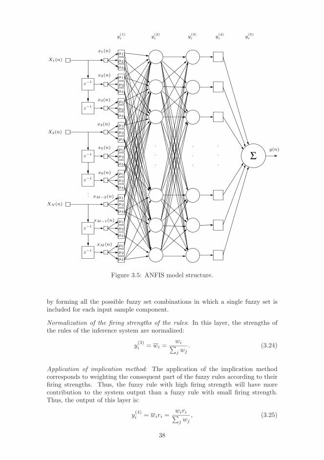
Σ

µ1

µ1

µ1

µ1

µ1

µ1

µ1

µ1

µ1

µ2

µ2

µ2

µ2

µ2

µ2

µ2

µ2

µ2

µ3

µ3

µ3

µ3

µ3

µ3

µ3

µ3

z−1

z−1

z−1

z−1

z−1

z−1

xM (n)

xM−1(n)

xM−2(n)

XN (n)

x6(n)

x5(n)

x4(n)

X2(n)

X1(n)

x3(n)

x2(n)

x1(n)

y(n)

µ3

y(2)i

y(1)i

y(4)i

y(5)i

y(3)i

Figure 3.5: ANFIS model structure.

by forming all the possible fuzzy set combinations in which a single fuzzy set isincluded for each input sample component.

Normalization of the firing strengths of the rules: In this layer, the strengths ofthe rules of the inference system are normalized:

y(3)i = wi =

wi∑

j wj. (3.24)

Application of implication method: The application of the implication methodcorresponds to weighting the consequent part of the fuzzy rules according to theirfiring strengths. Thus, the fuzzy rule with high firing strength will have morecontribution to the system output than a fuzzy rule with small firing strength.Thus, the output of this layer is:

y(4)i = wiri =

wiri∑

j wj, (3.25)

38

where the term wiri corresponds to the implication method.

Application of aggregation method: In this layer, the total output of the systemy(n) = y(5)(n) is computed as the average of the fuzzy rule outputs weighted bythe firing strengths of the rules. First, the consequent parts of the fuzzy rules areaggregated to form a single fuzzy set by summing the singleton spikes. Then, theresult of aggregation is defuzzified to form the numerical system output by dividingthe sum of weighted rule outputs by the sum of the firing strengths computed inthe normalization layer:

y(5) =∑

i

wiri =∑

i

wiri∑

j wj(3.26)

Thus, the concurrent application of firing strength normalization, fuzzy implicationand aggregation corresponds to the weighted average defuzzification method.

3.6 Clustering

Clustering of data means partitioning the data set into a set of clusters. Next, thek-means clustering algorithm and a validity index to choose the optimal clusteringis discussed. In addition, methods to allow easy analysis of cluster properties areoutlined.

3.6.1 k-means

One of the most widely used clustering method is the k-means algorithm (Everitt,1993; Hand et al., 2001; Bezdek and Pal, 1998). It belongs to the partitive clus-tering algorithms, that is, it divides the data into specified number of clusters (k)by minimizing

E =k

∑

i=1

∑

x∈Qi

||x− ci||2, (3.27)

where Qi denotes the ith cluster and ci denotes the center of the ith cluster. Thedefinition of distances used in clustering makes implicit assumptions about theshape of the clusters. The k-means searches for spherical clusters.

The basic version of k-means operates as follows: first, k cluster centers are pickedup in random fashion. Then, each sample in the data are assigned to the clusterwhose center is closest to the sample (typically, in the Euclidean sense). Then,the mean vector of the samples in the same cluster is computed and defined as thenew cluster centroid. These steps are iterated until memberships of the samplesin the clusters remain unchanged.

3.6.2 Davies-Bouldin Index

When using partitive clustering methods such as the k-means, it becomes necessaryto select the optimal number of clusters in which the data is divided. Several va-

39

lidity indices have been proposed. In this thesis, the Davies-Bouldin index (Daviesand Bouldin, 1979) minimizing

1

C

C∑

k=1

maxl 6=k

{

Sc(Qk) + Sc(Ql)

dce(Qk, Ql)

}

(3.28)

is used. In above, Sc denotes within cluster distance and dce denotes betweencluster distance. In the literature, other validity indices have been proposed. Formore information, see Bezdek and Pal (1998).

3.6.3 Cluster Description

In data analysis associated with clustering, it becomes useful to know what prop-erties are common in certain cluster and how the samples in a cluster differ fromthe samples in the other clusters. In this thesis, a cluster description algorithmpresented in (Siponen et al., 2001) is used.

Each rule produced by the algorithm describe clusters in terms of value ranges foreach measured variable. Single descriptive rules and their combinations for eachcluster can be computed by maximizing the significance measure Sr(i, r) of a ruler for cluster i:

Sr(i, r) = P (i|r)P (r|i) =n2

r&i

nrni, (3.29)

where nr is the number of data samples in the data set for which the rule r istrue, ni is the number of data samples in cluster i, and nr&i is the number of datasamples in the cluster i for which the rule r is true.

3.6.4 Clustering of SOM

In (Vesanto and Alhoniemi, 2000), a two-phase method for clustering is proposed.Firstly, a SOM is trained for a given (multivariate) data set. Then, a clusteringalgorithm is applied for the reference vectors (map unit locations in the measure-ment space) of SOM, instead of the original data set. In this approach, benefits ofSOM in multivariate data visualization are combined with the clustering method,providing an easy way to analyze the properties of the clusters. In addition, thisapproach provides computational efficiency for very large data sets, for which thedirect clustering would be very time consuming.

Several clusterings are performed, for example, with k-means algorithm and dif-ferent values for k and the best is selected according to the Davies-Bouldin index.

3.7 Segmentation

For the process monitoring purposes it is important to detect changes in the statis-tics of the measured data. In order to track such variations, a segmentation for the

40

time-series data can be obtained, and the properties of the segments can be stud-ied, for example, using different kind of visualizations. Next, the use of histogrammaps and operator maps in time-series segmentation is described.

3.7.1 Histogram maps

In (Raivio et al., 2001, 2003), a method for segmentation of time-series data wasproposed. In this method, the model for the segments is characterized by a distri-bution of the samples in a multivariate data space. In other words, the samplesof the sequences in the same segment are well described by the same distribution.For simplicity, the distributions are approximated by a histogram describing thenumber of samples in different clusters obtained with basic clustering algorithms.

In this method, the SOM is used to visualize the variety of histograms observedin the data. This is established by obtaining the initial clustering and then, per-forming histogram computation for each sequence of time-series data. Then, thehistogram data is visualized with the basic SOM algorithm.

Typically, the histogram data tends to form clusters of similar histograms. Thek-means algorithm can be used to link similar histograms and therefore, clusters ofhistograms can be obtained. The sequences of time-series data whose histogramsbelong the same cluster are declared to belong to the same segment.

Raivio et al. (2001, 2003) applied the segmentation method for the classificationof mobile cells into similarly behaving groups in order to obtain more efficientnetwork configuration optimization. In Publications 1 and 2, the histogram mapsare applied in mobile network performance monitoring problem.

3.7.2 Operator Maps

The basic SOM algorithm has been applied in many real-world data analysis prob-lems (Kohonen, 2001). However, the basic SOM algorithm is mostly useful incases where the data samples in the data set are statistically independent. Inmany process monitoring problems, the systems may be dynamical, that is, thepast measurements made from the system do have an influence on current systemoutput.

There are several generalizations of the basic SOM algorithm in which the mapunits of the SOM are considered as parametric models instead of static data pointsin the measurement space, resulting in so-called operator maps (Kohonen, 2001).The operators may be, for example, parametric probabilistic models (Hollmenet al., 1999) or dynamical models (Barreto and Araujo, 2000; Hyotyniemi et al.,1997; Lampinen and Oja, 1989). Such extensions of SOM are more useful in theanalysis of dynamical process data, and especially, in segmentation of process datain the form of time-series.

41

Usually, the SOM algorithms are based on gradient algorithms of the form

θ(t + 1) = θ(t)− α(t)∂E(t)

∂θ(t), (3.30)

where E(t) is the cost to be minimized (Kohonen, 1993). At each iteration t(epoch), the whole measurement data 1 ≤ n ≤ N is used to compute the updatedmodel parameter values, therefore, the learning occurs in batch mode. When themap units are considered to represent parameters of dynamical models, the errormeasure E(t) can be defined as the average prediction error of the model given thesystem input and true output y(n) for the system weighted over the neighborhoodhc(n),i(n, t) of the lattice of map units

E(t) =1

2N

∑

m∈L

N∑

n=1

hc(n),m(t, n)[y(n)− y(m)(t, n)]2, (3.31)

where y(m)(t, n) is the prediction of operator m for time point t for sequence n.

Note, that the winner search procedure in which the sequence c(n) for the neigh-borhood function is computed can be used to adjust the length of the subprocesssegments that are assumed stationary. For example, the map unit with smallestmean squared error over a process segment of length L and starting from timestep n0 can be declared as the winner unit for observations {xi(n), y(n)}, n =n0, n0 + 1, ..., n0 + L− 1.

In this thesis, several kind of parameterizations for the operators are used. Theadaptive filters are used as operators in order to obtain a segmentation basedon differences in linear dynamics in the process. The MLP networks are usedas operators in order to model nonlinear dynamics within the segments. Finally,ANFIS models are used for the same purpose as MLP operators. However, theANFIS operators enable the analysis of the nonlinear dynamical models in termsof fuzzy rules, being more useful for process monitoring purposes.

For operators consisting of adaptive filters, the output of the operator m is definedby:

y(m)(n) =

M∑

i=1

w(m)i xi(n), (3.32)

where M is the dimension of the input space, w(m)i is the ith weight of the mth

adaptive filter corresponding to the ith input variable xi(n). The advantages ofthis map unit parameterization are the easy interpretation of the model parametersas correlation between variables and the efficient optimization of the parameters.Since the model is linear in parameters, a solution corresponding to the globalminima can be obtained (for a single operational mode of the process).

In order to model any temporally local nonlinear dependence between the past andcurrent observations, the parameterization of the map units can be generalizedaccording to the MLP. In such a case, the output of the ith neuron in layer l of asingle operator m is

y(m,l)(n) = ϕ

Ml−1∑

j=0

w(m,l)ij y

(m,l−1)j (n)

, (3.33)

42

where y(m,l−1)j (n) is the jth input component for the neurons at layer l, w

(l)ij is

the jth synaptic weight of the neuron i at layer l, Ml−1 is the number of inputsfor layer l and ϕ is a nonlinear activation function. The main disadvantage of theMLP operators is the lack of interpretation for the estimated mapping.

In the analysis of spatio-temporal data, a human-comprehensible description aboutthe process is needed. An adaptive model suitable for this purpose is the ANFISmodel based on the zeroth-order Sugeno fuzzy inference system. In ANFIS, thedependence between the model input and output can be represented by a set ofhuman-friendly fuzzy rules of the form: if x1 is A and x2 is B then y is r, where Aand B are linguistic labels and r is a crisp consequent part parameter of the fuzzyrule. The output of an operator m in this case is:

y(m)(n) =

∑

k

∏

∀i,j∈Rmk

µ(m)ij (xi(n)) r

(m)k

∑

l

∏

∀i,j∈Rml

µ(m)ij (xi(n))

, (3.34)

where µ(m)ij (xi(n)) is the value of the jth premise part membership function for

the ith input component, r(m)k is the crisp consequent part parameter of kth rule

of the map unit m and Rmk is the set of premise part membership functions that

belong to the kth rule of the operator m.

Due to use of above mentioned nonlinear operators of different complexity, it wouldbe appropriate to include a mechanism to prevent the over-fitting of the map unitsinto the data in order to achieve better generalization capability. Thus, accordingto the regularization framework, an additional penalty term is added to the errormeasure to be minimized by the SOM

Er(t) =1

2N

∑

m∈L

N∑

n=1

[

hc(n),m(t, n)[

y(n)− y(m)(t, n)]2

+ λη[θ(m)]

]

(3.35)

where η(θ(m)) is the value of the parametric penalty function for the parametersof the mth map unit in the SOM and λ is the regularization parameter. Regular-ization can also be defined implicitly by using double resampling. In Publication3, the operator maps were used in mobile network performance analysis.

3.8 Knowledge Engineering

According to Ljung and Glad (1994), there are two sources of knowledge for sys-tem properties. Firstly, the collected experiences of application domain expertsand literature contain basic laws for the system operation. Secondly, the system it-self, and especially, the observations made from the system is an important sourceof information. The methods explained in the previous sections are heavily basedon using the measurement data from the system of interest. In this section, ap-proaches are presented in which prior knowledge outside the data records play animportant role in addition to the measurement data. In (Ljung and Glad, 1994),this is called knowledge engineering and it refers to tasks in which applicationdomain knowledge and mathematical model construction techniques are combinedin order to obtain knowledge-based models.

43

Examples of how prior knowledge can be used to focus on phenomena of interestinclude:

• selecting the most important variables from large amount of measurementdata depending on the problem at hand,

• selecting a subset of time points (samples) in which the variables meet certainstatic requirements,

• including constraints for dependencies between measured variables in orderto prune the amount of possible solutions, and

• deriving new mappings based on mathematical models in order to fill gapsbetween quantities of interest.

The use of application domain knowledge with the data-driven methods is stronglydependent on the problem at hand. In this chapter, only the principles of usingprior knowledge are outlined. The more detailed description of using prior knowl-edge is given in the next chapter of this thesis, in which the results of applyingdata driven methods to radio resource optimization problems are described.

3.8.1 Variable and Sample Selection

In modeling tasks, it is essentially important to use only the relevant variablesin modeling. In many cases, the variable selection problem can be attacked withmethods not requiring prior knowledge about the data (Guyon and Elisseeff, 2003).In many applications such as telecommunications, the variables tend to be verycolinear and correlate with the total amount of traffic in the system. In suchapplications, it is essentially important to know the meaning of the variables andto select the most relevant ones based on prior knowledge.

The simplest form of applying a priori information about the system in modelconstruction is the selection of the important variables for the problem at hand.This step is nearly always executed when data analysis methods such as neuralnetworks are used to process measurement data. In the analysis of data producedby networked systems, the topology and dependencies between individual datagenerating systems may be important to include in the system modeling. In thenetworked systems like wireless networks, this is especially important since geo-graphically close-by BTSs are usually connected into same controllers and also,many of the cellular network performance problems tend to be local in nature.For these reasons, many modeling problems require that variables from close-bycells are included in the same model. Similarly, it may be necessary to includevariables from other cells operating on the same frequency when building a modelfor a single BTS (see Publication 5).

In addition to the selection of important variables for the analysis, it is often usefulto focus on certain value ranges of the selected variables. Especially in telecom-munications, the KPIs have generally accepted thresholds that define the regionof acceptable performance. When analyzing process faults, it is natural to focus

44

on measurements in which acceptable performance is not met. In (Vehvilainen,2004), an example of data analysis method is given in which certain thresholds forimportant variables have been set and the data samples in which variables havevalues on the range of interest are taken into more careful analysis. In Publica-tion 4, a similar approach to select a subset of data for more careful analysis ispresented.

3.8.2 Constraining Dependencies between Variables

Sometimes, the prior information enables the simplification of the model estima-tion process by restricting the number of possible solutions. When building modelswith the counter data of the mobile networks, for example, it may become clearthat the regression model must not have any parameters having negative valuesnor values greater to one. In addition, it is very common that the sum of regres-sion model parameters must be equal to one. In Publication 5, such cases arise.In regression problems with such restrictions, the solution can be obtained withquadratic programming presented earlier in this thesis.

3.8.3 Importing Mathematical Models

In some cases, it is necessary to derive mappings between existing variables. Thederivation of the mappings is typically based on mathematical models describingapplication domain phenomena.

In (Oussar and Dreyfus, 2001), a semi-physical approach is presented in whichthe prior knowledge is in the form of continuous differential equations. Firstly,the continuous differential equations are discretized and then, the selected com-ponents of the discrete model are implemented by a neural network. The resultsof increasing the number and complexity of the neural network based componentsindicate that a model of increasing accuracy for the analyzed process is obtained.

Another approach of including prior knowledge is the case in which human expert isable to give simple, linguistic rules about how the system operates/should operatein some important operating regimes. These rules can be converted to fuzzy rulesand a fuzzy system can be obtained to perform the modeling or control task.In this case, the prior knowledge takes the form of rules, and no mathematicalcharacterization of the knowledge is needed.

In telecommunications, the use of mathematical models in combination with mea-surement data is a common practice. The most typical examples of mathematicalmodels in the telecommunication applications are path loss models and the Erlang-B formula describing the capacity of mobile networks. In Publication 6, a methodfor blocking prediction in GSM networks based on Erlang-B formula is presented.In Publication 7, the path loss models are used in prediction of signal quality andcall dropping in the context of cell size optimization. The use of path loss modelsallows the calculation of cell radius with different signal strength requirements.

45

Chapter 4

Data-Driven Radio Resource

Management

In this chapter, the results of applying data analysis methods and knowledge en-gineering techniques for the optimization of wireless network performance are pre-sented. Firstly, the results of visualization of multivariate performance data ofa 3G network simulations are discussed. Then, the results of performance anal-ysis using visualization are presented for operating GSM networks. Finally, thepredictive modeling approach for optimization of configuration parameters of anoperating GSM network is discussed.

4.1 Expert-Based UMTS Network Optimization

In this section, the results of applying data visualization to cellular network dataare presented. The purpose of the methods is to visualize useful information forhuman expert responsible for optimizing network performance. Since the taskis usually associated with multiple performance measures and reasonable overallperformance is of interest, this step reduces to visualization of multivariate data.

4.1.1 Network Scenarios

The UMTS network analysis is performed for two network plans. Firstly, a mi-crocellular network scenario consisting of 46 base stations with omnidirectionalantennas was analyzed. The network scenario is depicted in Figure 4.1. The datafrom this network scenario was analyzed in Publication 1 with the histogram map,the focus being on the analysis of downlink (BS to MS) performance of this net-work. In Publication 2, the analysis of this network scenario focused on the uplink(MS to BS) performance monitoring.

The second network plan consisted of 31 base stations with sector antennas and one

46

Figure 4.1: Microcellular network scenario with 46 base stations with omnidirec-tional antennas.

Figure 4.2: Macrocellular network scenario with 31 base stations with sector an-tennas and one omnidirectional antenna.

base station with omnidirectional antenna. This macrocellular network scenario isdepicted in Figure 4.2. This network scenario was analyzed in Publication 3 withthe operator maps. In these analysis, the focus was on the downlink performance.

4.1.2 Cell Monitoring

When a large data record describing the operation of wireless network is at hand,it is natural to question how it should be used in order to analyze how the networkis operating. For this purpose, a some kind of description about process statesand their variations should be obtained, for example, in graphical form in orderto provide this information for human expert. Next, three approaches to definea process state and to estimate the process states in different time segments arepresented (see Section 3.7).

47

(a) (b)

Figure 4.3: (a) Visualization of data clusters and (b) their properties using SOM.

Histogram Map

In Publication 1, the problem of monitoring the state of the cells in a microcellularUMTS network scenario was studied with the use of histogram map. The focuson downlink performance of the network. Firstly, the most important variablesfrom all the 46 cells were used to train a SOM. These include the number ofusers (nUsr), downlink transmission power (dlTxp) and downlink frame error rate(dlFER). Then, the codebook of the SOM was clustered into five clusters usingk-means clustering algorithm. Figure 4.3(a) shows the trained SOM and how theSOM grid is separated into clusters obtained with the k-means algorithm. Therules describing the clusters in the measurement space are shown in Fig. 4.3(b).From the rules it easy for application domain expert to assess the properties of eachdata cluster. For example, cluster 4 represents data samples with unacceptablehigh downlink frame error rate (dlFER > 0.05).

In order analyze slow variations in the behavior of the mobile cells, segmentation forthe time-series data was performed. The histogram map was used in segmentationby first dividing the data into sequences of equal length, and computing the numberof samples in previously computed clusters for each of the data sequence. Thehistograms of the sequences were used to train the histogram map.

Similarly to the SOM trained with the mobile network data, the histogram mapcan be clustered in order to obtain the segmentation of the time-series data. Thetrained histogram map was clustered into seven clusters using the k-means clus-tering algorithm in order to separate dissimilar areas on the map. Figure 4.4(a)shows the clustered histogram map.

48

(a) (b) (c)

(d) (e) (f)

Figure 4.4: (a) Clusters on the histogram map and (b) their properties visualizedby histograms. (c) Properties of clusters are manually labeled on top of SOM.Trajectories of mobile cells (d) 8, (e) 14 and (f) 44 of the mobile network on thehistogram map.

In Figure 4.4(b) the properties of each cluster on the histogram map are shown.Each cluster represents differently distributed data samples in the measurementspace. These distributions are visualized as a data histogram in which each barrepresents the density (occurrence probability) of the corresponding data cluster inthe measurement space. For example, cluster 6 on the histogram map representsdensity structures in which most of the data samples are located in data cluster4 as indicated by the height of the 4th bar of the histograms. As mentionedearlier, the data cluster 4 represents data samples with unacceptable high downlinkFER, indicating that cluster 6 on the histogram map describes undesired datadistribution and thus it should be avoided by making corrections to the processconfiguration parameters. In Figure 4.4(c), the histogram map in which the clusterproperties are manually labeled on the map is shown.

In order to monitor the behavior of the mobile cells, the trajectory of the map unitson the histogram map that best describe the state of the consecutive sequences

49

of the cell data can be visualized. By following the trajectory, the changes in cellbehavior are easily detected. Figures 4.4(d)-(f) illustrates this monitoring processfor mobile cells 8, 14 and 44. For example, cell 8 starts from low load state, visitingmedium load and high load areas before settling back to medium load area. Mobilecell 14 operates on low load, except a small peak in dlFER in the beginning of thedata set. Cell 44 operates exclusively on high load and dlFER area.

In Publication 2, similar analysis was performed for the uplink data of the samenetwork scenario. In addition, the presented results were compared with tradi-tional network analysis based on uplink loading equations.

Linear Operators

A second approach to cell monitoring is based on tracking the changes in lineardynamics in the cells. This was based on the use of operator maps in which theoperators were adaptive linear filters (see Publication 3). In Figure 4.5(a) theparameters of the adaptive filters of the [4× 4] operator map are shown. Each barof the histogram indicates the value of a single parameter of the correspondingmodel. The first bar corresponds to the coefficient of the non-delayed sampleof the number of users and the second bar corresponds to the coefficient of thefirst delayed sample of the number of users. The third bar corresponds to thenon-delayed sample of downlink average transmission power, and the fourth barcorresponds to the delayed sample of the downlink average transmission power.The last bar indicates the bias term of the model, that is, the mean of the outputprocess (downlink frame error rate).

From the figure it can be seen that the parameters of the map are topologicallyordered since the neighboring map units do have similar values for the parameters.Three clearly different areas can be found on this map: the map units in theupper left corner have the highest values for the coefficients corresponding to thecurrent and past values of the number of users in the network. That is, the moreusers the mobile cell has, the worse is the quality of the service provided by thecell since there is a strong positive correlation between the number of users andthe downlink frame error rate. In contrast, the coefficients corresponding to thedownlink average transmission power tend to have small negative values. In otherwords, high values of the downlink average transmission power tend to have a weaklowering effect on the downlink frame error rate.

The upper right corner of the map represents similar behavior, except that theframe error rate is not well explained by the changes in the downlink averagetransmission power. This is due to the fact that the values of the correspondingparameters are nearly zero. Thus, the only conclusion that can be made is thatthe higher the number of users in the cell is, the higher is the frame error rate.

The lower half of the map consists of models with small positive values for allparameters, stating that both the number of users and the downlink average trans-mission power correlate positively with the frame error rate. Thus, the bad qualitycan up to some level be explained by the number of users, but an increase in trans-mission power does not seem to produce better performance.

50

(a)

Cell 1

(b)

Cell 4

(c)

Cell 9

(d)

Figure 4.5: (a) Parameters of the adaptive filters of the operator map. The tra-jectories of the cells (b) 1, (c), 4 and (d) 9 of the mobile network.

The visualization of the parameters of the adaptive filters as shown in Figure 4.5(a)can be used to examine the spectrum of the data generating models in a piecewisestationary process. Similarly to the histogram map based visualization, the tra-jectories of the mobile cells on the operator map can be used to analyze long-termvariations in the cells. In Figures 4.5(b)-(d), examples of such trajectories havebeen shown. In cell 1, the variation in performance can be explained only in termsof the high number of users, since they visit the upper right corner of the map.Cell 4 is an example of base station in which the bad performance occurs when thenumber of users is high, but the increase of the downlink transmission power doesnot seem to help in reaching the network users. Cell 9 suffers from a decrease inperformance when the number of users is high and the average transmission powertoo low since they visit the upper left corner of the operator map.

Non-Linear Operators

The third approach for cell monitoring is based on operator maps in which theoperators are simple ANFIS models (see Publication 3). For purposes of networkplanning, it is of interest to know when the cells generate high values for the frameerror rate. Thus, the analysis of the rule plane shown in Figure 4.6(a) can be usedto track the conditions for various quality problems. For example, the map units{6, 7, 11} tend to produce high FER values when the number of users in the cell islow. At the same time, the number of users in the past were high, indicating thatthe bad performance occurs when the number of users drops. In map units {7, 11},

51

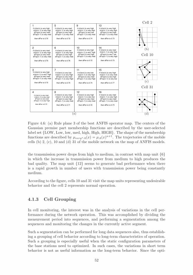
if nUsr(n) is very high nUsr(n−1) is very high dlTxp(n) is very med

dlTxp(n−1) is very med

then dlFer is 0.70

1

if nUsr(n) is very med nUsr(n−1) is very high dlTxp(n) is very med

dlTxp(n−1) is very med

then dlFer is 0.70

2

if nUsr(n) is very high

nUsr(n−1) is very2 high

dlTxp(n) is very med dlTxp(n−1) is very med

then dlFer is 0.72

3

if nUsr(n) is very med nUsr(n−1) is very med dlTxp(n) is very med

dlTxp(n−1) is very2 high

then dlFer is 0.72

4

if nUsr(n) is very med nUsr(n−1) is very high dlTxp(n) is very high

dlTxp(n−1) is very med

then dlFer is 0.72

5

if nUsr(n) is very low nUsr(n−1) is very high dlTxp(n) is very high

dlTxp(n−1) is very med

then dlFer is 0.76

6

if nUsr(n) is very low nUsr(n−1) is very High dlTxp(n) is very med

dlTxp(n−1) is very High

then dlFer is 0.70

7

if nUsr(n) is very med nUsr(n−1) is very high dlTxp(n) is very high

dlTxp(n−1) is very med

then dlFer is 0.71

8

if nUsr(n) is very high nUsr(n−1) is very high

dlTxp(n) is very low dlTxp(n−1) is very med

then dlFer is 0.74

9

if nUsr(n) is very high

nUsr(n−1) is very2 high

dlTxp(n) is very high dlTxp(n−1) is very med

then dlFer is 0.72

10

if nUsr(n) is very low nUsr(n−1) is very high dlTxp(n) is very med

dlTxp(n−1) is very High

then dlFer is 0.74

11

if nUsr(n) is very high nUsr(n−1) is very low dlTxp(n) is very med

dlTxp(n−1) is very med

then dlFer is 0.72

12

if nUsr(n) is very high nUsr(n−1) is very high dlTxp(n) is very high

dlTxp(n−1) is very med

then dlFer is 0.73

13

if nUsr(n) is very med nUsr(n−1) is very high

dlTxp(n) is very2 low

dlTxp(n−1) is very high

then dlFer is 0.73

14

if nUsr(n) is very high nUsr(n−1) is very med dlTxp(n) is very high

dlTxp(n−1) is very low

then dlFer is 0.77

15

if nUsr(n) is very med nUsr(n−1) is very high dlTxp(n) is very med

dlTxp(n−1) is very med

then dlFer is 0.73

16

(a)

Cell 2

(b)

Cell 10

(c)

Cell 31

(d)

Figure 4.6: (a) Rule plane 3 of the best ANFIS operator map. The centers of theGaussian premise part membership functions are described by the user-selectedlabel set {LOW, Low, low, med, high, High, HIGH}. The shape of the membershipfunctions are described by µverynA(x) = µA(x)n+1. The trajectories of the mobilecells (b) 2, (c), 10 and (d) 31 of the mobile network on the map of ANFIS models.

the transmission power drops from high to medium, in contrast with map unit {6}in which the increase in transmission power from medium to high produces thebad quality. The map unit {12} seems to generate bad performance when thereis a rapid growth in number of users with transmission power being constantlymedium.

According to the figure, cells 10 and 31 visit the map units representing undesirablebehavior and the cell 2 represents normal operation.

4.1.3 Cell Grouping

In cell monitoring, the interest was in the analysis of variations in the cell per-formance during the network operation. This was accomplished by dividing themeasurement period into sequences, and performing a segmentation among thesequences and monitoring the changes in the currently active segment.

Such a segmentation can be performed for long data sequences also, thus establish-ing a grouping of cell behavior according to long-term characteristics of operation.Such a grouping is especially useful when the static configuration parameters ofthe base stations need to optimized. In such cases, the variations in short termbehavior is not as useful information as the long-term behavior. Since the opti-

52

(a) (b)

Figure 4.7: (a) Clusters, (b) classification of mobile cells.

mization of the mobile network parameters cell by cell can be very time consuming,the cell grouping can be efficiently used to simplify the optimization task. In otherwords, the mobile network parameter optimization reduces to optimization of theparameters of the clusters of cells instead of cell by cell (Laiho et al., 2002c) sothat the cells in the same cluster have the same configuration parameters. Thehistogram map and the operator maps described in the previous section can beused to obtain this cell classification.

In Publication 2, the histogram map was used to obtain the cell grouping. InFigure 4.7(a), the clustered histogram map used for cell grouping is depicted.This classification is based on uplink data of the microcellular network scenario.The histogram map consists of 8 behavioral clusters, each indicated by a differentgray-level. In Figure 4.7(b), the map units best describing the data from differentmobile cells are shown.

4.2 Expert-Based GSM Network Optimization

4.2.1 A SOM Based Visualization Process

In Publication 4, a SOM based analysis process to track performance bottlenecksin operating GSM network was presented. The proposed SOM based analysisprocess is illustrated in Figure 4.8. In this study, the KPI data from the GSMnetwork was studied. The network consisted of 41 base stations from which themost important KPIs over 10-week time period were measured.

When projection methods such as the SOM are used in data visualization, all

53

Data selection SOM Clustering Visualization

Figure 4.8: A block diagram illustrating the phases of the proposed analysis pro-cess.

samples usually have equal priority when determining the projection (dimension-ality reduction) function. In order to focus on certain network problem types, thesamples representing normal operation can be removed before the more detailedanalysis. When analyzing the performance degradations of a GSM network, themost important samples can be selected by choosing the KPIs of interest and re-taining only the samples for which the operator defined objective values are notmet. For example, if an accurate visualization of traffic channel problems aredesired, it would be justified to use only the samples in which traffic channel orsignaling channel blocking occurs, or traffic channel drop rate exceeds 2%.

After the subset of data of interest is selected, the data is normalized in orderto make all variables equally important independently on the measurement unit.Then, the normalized data is used as the input data in SOM training. The trainedSOM is used to visualize the multi-dimensional input data using the componentplane representation of SOM.

As mentioned earlier in the thesis, clustering can be used to divide performancedata into different clusters representing different types of failures. In this study,the approach presented in Section 3.6.4 was adopted in which the clustering isperformed for trained SOM in order to provide simple visualization of clusterproperties. After the SOM training and clustering, a visualization of the selectedmulti-dimensional input data is obtained. This information helps the applicationdomain expert to make inferences about the possible problem scenarios present inthe data. The cluster analysis based on SOM component planes reveals the varietyof failures faced by the network. It is relatively easy task for an expert to select themost important variables (KPIs) for each failure type. By analyzing the amount ofsamples in different fault clusters originating from each cell of the GSM network,the locations of the different failure types are efficiently obtained. Finally, thevisualization of the times of occurrence of different fault types reveals additionaltemporal information about the faults. These three types of simple visualizationsallows the selection of variables, cells and time periods that are taken into furtheranalysis using conventional methods.

In the analysis of SDCCH problems in the network, the samples meeting therequirement SDCCH Blocking > 0 % was used in order to filter the uninformative(normal operation) samples from the analysis. Then, histogram equalization basednormalization method were applied for the selected data set in order to obtaininvariance w.r.t the scales of the variables. Then, a SOM was trained in which themap units were organized in a [15× 10] hexagonal grid by applying 500 epochs of

54

0.0262

0.216

0.405

d 0.121

4.3

30.3Sdcch Block

d 0.38

5.76

100Sdcch Avail

d 0

0

1Ul SQl

d 0

1

1Dl SQl

d 105

108

110Ul SS

d 107

108

110Dl SS

d 0.000679

0.0453

0.469Cs Traffic U−matrix

77

73

33

44

44

44

11

1

77

73

33

44

44

44

11

1

77

33

33

44

44

44

11

1

73

33

33

44

44

44

11

1

33

33

33

32

44

45

55

1

33

33

32

22

22

55

55

5

66

33

32

22

22

55

55

5

66

62

22

22

22

55

55

5

66

66

22

22

22

55

55

5

66

66

22

22

22

55

55

5

Figure 4.9: SOM of data samples representing possible signaling channel capacityproblems. Clusters 1, 4, 6 and 7 represent possible signaling channel capacityproblems.

batch training and 500 epochs of sequential training.

In Figure 4.9, the so-called component planes of the SOM are shown (Vesanto,1999). In addition to reveal the cluster structure, the cluster indices of the mapunits obtained with the k-means are shown along with the visual U-matrix repre-sentation of SOM (Ultsch and Siemon, 1990).

By analyzing the properties of each cluster using the component planes, four clus-ters that represent possible signaling channel capacity problems can be identified:cluster 4 contains high values for signaling channel blocking, with moderate amountof traffic. Clusters 1 and 6 represent behavior in which a drop in channel avail-ability is likely to cause the high blocking values. Cluster 7 represents channelblockings that are likely to be a result of bad signal quality, i.e. the connectionis refused because the required channel quality could not be provided. The U-matrix reveals that the clusters 1, 6 and 7 are located further apart from the otherclusters.

The locations of the various fault types can be analyzed by computing the numberof hits into different fault clusters (see Figure 4.10(a)). From the figure, it becomesevident that nearly all of the samples in the fault clusters were generated byonly three cells of the network. Hits from other cells can be viewed short-termfailure situations that do not give reasons to major configuration adjustments and

55

1 3 5 7 9 11 13 15 17 19 21 23 25 27 29 31 33 35 37 39 410

2

4

6

8

10

12

Number of hits to clusters

Cluster 1Cluster 4Cluster 6Cluster 7

(a)

19/01 24/01 29/01 03/02 08/02 13/02 18/02 23/020

0.5

1

1.5

2

2.5

3Number of hits to clusters

Cell 12, cluster 1

(b)

Figure 4.10: (a) Cells 12, 15 and 16 contribute the most to the fault clusters. (b)In cell 12, the failures appear mostly during a 4-day period.

therefore can be ignored.

When plotting the times of occurrences of the hits to the fault clusters from thesethree cells, it was found that the cell 12 had a 4-day period when most of thesamples into fault cluster 1 were generated (see Figure 4.10(b)). This suggeststhat the signaling channel availability were temporarily reduced (i.e. the amountof available channels dropped) and therefore, some of the channel requests wereblocked. In order to verify this assumption, it was easy to plot the variable de-scribing the number of available SDCCH channels against the number of blockedSDCCH requests during that 4-day time period. After this simple plotting, it waseven more clear that it is the drops in availability that causes the requests to be

56

blocked. This procedure is a good demonstration that failures related to multiplevariables can be easily found, the base stations and the time periods in which theyoccur is easy to obtain and verifying plots are straightforward to accomplish withthis kind of analysis procedure.

In Publication 4, the same analysis procedure was followed for the analysis ofTCH capacity problems in the same network. Several interesting failure situationswere found from the data. Firstly, the drop in channel availability in close-bycells was detected. In addition, blocking problems in two cells due to the lack ofresources were detected. In addition, interesting relationships between cell size andcall dropping were found, stating that high call dropping rate is often observed insmall cells and during time periods with low amount of traffic.

4.2.2 A Knowledge-Based Visualization Process

In previous section, the analysis of GSM network performance was based on KPIdata. Also, the main objective have been in detecting the type and geographicallocation of the performance bottlenecks. The network analyzer have been respon-sible for analyzing the cause of the performance problems. In this section, theperformance is analyzed using the raw counter data. By using the counter data,the possible causes for the performance problems can be tackled more automati-cally based on observations, which is not possible on the basis of KPI data.

In Publication 5, a multi-layer hierarchical structure of cause-effect pairings weredeveloped. The set of available measurements were assigned into variable groupsbased on a priori knowledge about the semantics of the variables. Within a variablegroup, the variables are clearly connected while the variables from different groupsare independent on each other. Therefore, the modeling problem is more easilysolved by identifying a separate subsystem for each variable group separately.

In Figure 4.11(a), the memberships of the variables in different groups (subsystems)are shown. This plot shows the set of input variables (gray) and output variables(black) that belong to each of the subsystems (y-axis). The subsystems tend toform a hierarchical structure (see Figure 4.11(b)), i.e. the outputs of a subsystemdescribing some low-level phenomena can be an input to a higher-level subsystem.In the figure, the solid lines indicate that the input of the upper level systemcontains outputs of the lower level system from the same BTS only. The dashedline indicates, that the input of the upper level system contains input signals fromlower level systems of the other BTSs also.

For each variable group, a simple constrained optimization problem with suitableconstraints were defined. In Table 4.1, the different types of models and thecorresponding constrained optimization problem for the subsystems are shown.For different model types, a priori knowledge about the associated variables wasused to determine the constraint equations and, for example, the presence of biasin the model.

Once the model parameters were estimated from the data, the cause-effect chainsrelated to performance degradations in the network can be analyzed using themodel parameters. In order to visualize the most interesting and useful cause-

57

Variables10 20 30 40 50 60 70 80 90 100

S 1,1 S 2,1 S 2,2 S 2,3 S 2,4 S 3,1 S 3,2 S 3,3 S 5,7 S 5,8 S 5,9 S 5,10S 5,11S 5,12S 4,1 S 4,2 S 4,3 S 5,5 S 5,4 S 6,8 S 5,2 S 5,3 S 6,1 S 6,2 S 6,3 S 6,4 S 6,5 S 6,6 S 7,1 S 6,9 S 6,10S 7,2 S 7,3

(a)

S 1,1

S 2,3S 2,2S 2,1 S 2,4

S 3,3S 3,2S 3,1

S 4,1S 4,2S 4,3

S 5,12S 5,11

S 7,2

S 5,8S 5,7 S 5,9 S 5,10

S 6,9 S 6,10

S 7,3

S 5,5 S 5,2 S 5,3 S 5,4

S 6,1 S 6,2 S 6,3 S 6,4 S 6,5 S 6,6 S 6,8

S 7,1

(b)

Figure 4.11: (a) Input and output variables (x-axis) of different subsystems (y-axis). (b) The subsystem hierarchy.

effect chains, a list of strong dependencies was obtained. An item to a dependencylist is generated per each input-output variable pair, including the strength of thedependency between the input and output variable (the value of the parametera), a measure of model accuracy (root mean square prediction error (RMSE) ofthe model), and a measure of models importance in overall network performanceanalysis (the average number of failures stored in the output variable of the input-output variable pair).

After all the models have been estimated and the properties of each input-outputvariable pairs are stored in the dependency list, a tree-shaped graph is constructedin order to analyze the cause-effect chains generating the major performance degra-dations of the network. Since the number of theoretically possible dependencies isextremely large, only the most important dependencies are included to the depen-

58

Table 4.1: The different types of models for the subsystems.

Type Systems Model Parameter estimation

S1,1, S2,1,S2,2, S2,3,

I S2,4, S3,1, y(t) =P

ixi(t) ai =

P

txi(t)/

P

ty(t)

S3,2, S3,3

S5,7, y(t) = ax(t) + b mina12 aT XT Xa− yT Xa

II S5,8, = [ a b ]

»

x(t)1

–

a1 ∈ [0, 1]

S5,9 = aT x(t) a2 ≥ 0

S5,10, S5,11, y(t) = aT x(t) + b mina12 aT XT Xa− yT Xa

III S5,12, S6,9, = [ a b ]

»

x(t)1

–

P

i6=Nai = 1,

S6,10, = aT x(t), ai6=N ∈ [0, 1]S7,1 aN ≥ 0

S4,1, S4,2

S4,3, S5,2,

S5,3, S6,1, minA

P

i12AT

i XT XAi − yTi XAi

IV S6,2, S6,3, y(t) = x(t)A,P

iaij = 1,

S6,4, S6,5, aij ∈ [0, 1]S6,6

S5,4, y(t) = a1(c1(t) + c2(t) + c3(t))x1(t) mina12aT XT Xa− yT Xa

V S5,5, +a2(c1(t) + c2(t) + c3(t))x2(t)P

iai = 1,

S6,8 +a3(c1(t) + c2(t) + c3(t))x3(t), ai ∈ [0, 1]

dency tree.

Three criteria are used to prune uninteresting dependencies from the tree. Firstly,the model accuracy from which the dependency originates must be at a reasonablelevel. Otherwise, the analysis might be misled by very inaccurate models havinglarge values for parameter a (which is forced in several models due to the equalityconstraints for the parameter vector). Secondly, the output variable of the de-pendency must be interesting enough (i.e relatively large number of failures mustbe observed in the output variable). Finally, only the dependencies that belongto the cause-effect chains contributing most to the overall network performancedegradations are included into the dependency tree. For each subsystem, differentminimum and maximum values for strength of dependency, model accuracy andmodel interestingness are defined.

Figures 4.12(a)-(d) show the pruned dependency trees in four separate cases. InFigure 4.12(a), the cause-effect chains of the most significant blocking problems areshown. Clearly, there are 4 BTSs (6,11,18,85) that suffer from lack of resources.BTSs (6,11,18) suffer from lack of half rate traffic channels and BTS 85 suffersfrom lack of full rate traffic channels. Only BTS 6, the causes for blocking can besaid to result regularly from congestion.

In Figure 4.12(b), the results of the corresponding analysis for the call setup failuresare shown. Here, four BTSs (17,52,66,74) seem to suffer from call setup failuresregularly. In all these four BTSs, the failures tend to originate during SDCCHsignaling and fail due to radio link problems. In BTSs 17 and 74 the radio linkfailures can be said to result from bad downlink signal quality and in BTSs 52 and66 they are due to bad uplink signal quality.

Figure 4.12(c) shows the corresponding results for call dropping problems. Again,the cause-effect chains for describing the reasons for dropped calls in four BTSs

59

blo

ckin

g 8

5

blo

ckin

g 6

blo

ckin

g 1

1

blo

ckin

g 1

8

tch

rej re

q d

ue

lack fr 8

5

tch

rej re

q d

ue

lack h

r 6

tch

rej re

q d

ue

lack h

r 11

tch

rej re

q d

ue

lack h

r 18

tch

req

du

ring

hr c

on

ge

stio

n 6

(a)

ave

dl s

ig q

ua

l 12

17

ave

dl s

ig q

ua

l 2 7

4

ave

dl s

ig q

ua

l 3 7

4

ave

dl s

ig q

ua

l 4 7

4

ave

dl s

ig q

ua

l 6 1

7

ave

ul s

ig q

ua

l 11

52

ave

ul s

ig q

ua

l 6 6

6

ca

ll se

tup

failu

re 5

2

ca

ll se

tup

failu

re 6

6

ca

ll se

tup

failu

re 7

4

ca

ll se

tup

failu

re 1

7

sd

cch

fails

52

sd

cch

fails

66

sd

cch

fails

74

sd

cch

fails

17

sd

cch

rad

io fa

il 52

sd

cch

rad

io fa

il 66

sd

cch

rad

io fa

il 74

sd

cch

rad

io fa

il 17

(b)

ave

bu

sy tc

h 5

6

ave

bu

sy tc

h 6

9

ave

bu

sy tc

h 8

3

ave

bu

sy tc

h 1

ave

bu

sy tc

h 6

ave

ul s

ig q

ua

l 1 6

ave

ul s

ig q

ua

l 10

69

ave

ul s

ig q

ua

l 11

69

ave

ul s

ig q

ua

l 4 6

ave

ul s

ig q

ua

l 5 6

ave

ul s

ig q

ua

l 7 6

9

ave

ul s

ig q

ua

l 8 6

9

ave

ul s

ig q

ua

l 9 7

dro

pp

ed

ca

lls 6

9

dro

pp

ed

ca

lls 7

4

dro

pp

ed

ca

lls 6

dro

pp

ed

ca

lls 7

tch

rad

io fa

il 69

tch

rad

io fa

il 74

tch

rad

io fa

il 6

tch

rad

io fa

il 7

(c)

bsc i fa

il lack 8

5

bsc i fa

il lack 6

bsc i fa

il lack 1

1

bsc i s

dcch

tch

at 6

b

sc i tc

h tc

h a

t 6

bsc i tc

h tc

h a

t 11

bsc o

ha

nd

ove

r failu

res 9

0

bsc o

ha

nd

ove

r failu

res 7

bsc o

ha

nd

ove

r failu

res 9

bsc o

tch

tch

at 7

bsc o

tch

tch

at 1

2

bsc o

tch

tch

at 1

8

ca

use

do

wn

lev 1

2

ca

use

do

wn

lev 1

8

ca

use

do

wn

qu

al 1

2

ca

use

do

wn

qu

al 1

8

ca

use

pb

dg

t 12

ca

use

pb

dg

t 18

ca

use

up

leve

l 12

ca

use

up

leve

l 18

ca

use

up

qu

al 1

2

ca

use

up

qu

al 1

8

ha

nd

ove

r failu

res 9

0

ha

nd

ove

r failu

res 7

ha

nd

ove

r failu

res 9

(d)

Figure 4.12: The analysis of the four main components of the user perceivedquality. (a) Cause-effect chains for blocking of services, (b) call setup failures, (c)call dropping and (d) handover failures.

(6,7,69,74) are shown. The reasons for call dropping seem to be radio link failures.In BTSs 6, 7 and 69 the radio failures are likely due to bad signal quality in uplink.In two TRXs of BTS 6 and in one TRX of BTS 69 the number of bit errors seem tocorrelate with the amount of traffic in both the own BTS as well as in interferingTRXs on the same radio frequency.

Finally, in Figure 4.12(d) the analysis of the handover problem sources are shown.The results for three BTSs (7,9,90) having the worst handover performance areshown, indicating that the problems are in BSC controlled outgoing handovers. InBTSs 7 and 9, the problems seem to be in lack of resources in the target BTSs(6,11,85). In target BTS 6 suffering from lack of resources, there seems to be highamount of incoming TCH-TCH handover attempts from BTS 7. This same BTStend to cause problems also for target BTS 11 suffering from lack of resourcesduring handover attempts. For target BTS 11, two other BTSs (12,18) are foundthat can be said to generate high number of handover attempts. The handoverattempts of these two BTSs are due to very similar reasons: the quality of theuplink and downlink radio connection and the uplink and downlink signal strengthare not reasonable in these two BTSs, and some of the users are switched into moreappropriate BTSs. Also, significant number of users are switched to another BTSin order to minimize the energy consumption of the MSs (power budget).

60

This study is a good indication of how a priori knowledge can be used to ease themodel estimation by pruning variables. Only the theoretically sound dependenciesneed to be estimated. Then, regression techniques can be used to estimate thestrength of the theoretically possible dependencies, and only the strongest onesare taken into more careful analysis. The possible dependencies between cells canbe analyzed by including variables from other cells to the models. The presentedmethod allows efficient fault detection, identification of strongest input variables,and diagnosis of the causes of the faults.

4.3 Predictive GSM Network Optimization

In previous sections, methods for fault detection, identification and fault diagnosishave been discussed. In this section, the focus is on the final step of the processmonitoring procedure, that is, on the process recovery. In the context of mobilenetwork performance monitoring, the process recovery is associated with mak-ing adjustments to configuration parameters so that the amount of predictable,regularly occurring performance degradations or faults is minimized. In order toautomate the configuration parameter optimization, a computational method toevaluate the performance of alternative configurations must be available. In data-rich environments like cellular networks, such predictive models are most efficientlyobtained with the use of past data records. Next, the data analysis methods andsuitable knowledge engineering approaches are used to build predictive models thatcan be used in automated configuration parameter optimization.

4.3.1 Prediction of Blocking

In blocking prediction, the interest is to compute the number of blocked requestsat different conditions. This can be based on the use of well known Erlang-Bformula. The expected value for the number of blocked requests is obtained bymultiplying the number of arriving requests with the blocking probability givenby Equation 2.4, leading to B = λp(Nc|λ, µ,Nc). The expected value for thecongestion time is C = p(Nc|λ, µ,Nc) and the expected value for the number of

channels in use is M =∑Nc

n=0 np(n| λ, µ,Nc).

In Publication 6, it was shown that the Erlang-B formula does not provide accuratepredictions for blocking in GSM networks if low sampling rate measurements ofarrival process are used in the model. More traditional regression methods can beused for the same purpose with the assist of knowledge engineering approach inwhich Erlang-B formula and regression methods are combined. With the use ofErlang-B formula, the dependencies between B,C and M that remain the samein each base station system need not be estimated from data alone. The data canbe used to estimate other relevant and additional parameters that are requiredin prediction. In Publications 6 and 7, a method to use Erlang-B formula andmeasurement data to predict blocking is presented. The regression techniquesare used to estimate the arrival rate distribution describing the arrival processduring short time periods. The Erlang-B formula is used to compute the amount

61

of blocking during the short time periods.

Suppose that the time period is divided into Ns segments of equal length. Also,assume that we have a vector λ = [0 1∆λ 2∆λ . . . (Nλ − 1)∆λ] of Nλ possiblearrival rates per segment with discretization step ∆λ. Let us denote the number ofblocked requests during a segment with arrival rate λi with Bi = λip(Nc|λi, µ,Nc),where p(Nc|λi, µ,Nc) is the blocking probability given by the Erlang distribu-tion. Also, the congestion time and the average number of busy channels dur-ing a segment with arrival rate λi are denoted with Ci = p(Nc|λi, µ,Nc) and

Mi =∑Nc

n=0 np(n|λi, µ,Nc). In other words, the segment-wise values for blockedrequests, congestion time and average number of busy channels are based on theErlang-B formula.

Now, assume that the number of segments with arrival rate λi is θi and∑

i θi = Ns.Then, the cumulative values over one hour for the number of requests T , blockedrequests B, congestion time C and average number of busy channels M can becomputed with

λ1 λ2 . . . λNλ

B1 B2 . . . BNλ

C1

Ns

C2

Ns. . .

CNλ

Ns

M1

Ns

M2

Ns. . .

MNλ

Ns

θ1

θ2

...θNλ

=

TBCM

(4.1)

or in matrix notation Xθ = Y.

Now, the problem is that the vector θ is unknown and it must be estimated fromthe data using the observations of Y and matrix X which are known a priori.Since the output vector Y includes variables that are measured in different scales,it is necessary to include weighting of variables into the cost function. By selectingvariable weights according to their variances estimated from the data, the quadraticprogramming problem

minθ

{

1

2θ

T Hθ + fTθ

}

(4.2)

w.r.t 0 ≤ θi ≤ Ns, i = 1, 2, ..., Nλ, (4.3)Nλ∑

i=1

θi = Ns (4.4)

is obtained where f = −XT WT WY and H = XT WT WX include the weightingmatrix W. In other words, the goal is to find the vector θ that provides the smallestprediction errors for variables T,B,C and M . For many BTSs, the number ofblocked requests B and the congestion time C are regularly zero and the use ofthe corresponding rows in X and Y is not possible due to the numerical problemsoccurring in the optimization. In such cases, the solution vector θ can be solvedusing only the two remaining rows of X and Y.

Now, suppose that we have Nd observations for variables T,B,C and M , all mea-sured at hour h during different days. The above optimization problem could besolved for each of the Nd observation vectors separately, leading to Nd solutionvectors θ for hour h. Since we are interested in long-term prediction of blocking,

62

we should somehow combine the solution vectors so that behavior common to allsolution vectors are retained and non-regular properties of the demand are givenless attention.

Let us denote the ith solution vector for hour h with θ(i)h and the jth element of

the corresponding solution vector with θ(i)jh . Since θ

(i)jh described the number of

segments with arrival rate λ = λj during ith observation vector at hour h, theprobability for a random segment during ith observation period to have an arrival

rate λ = λj can be computed from θ(i)jh with p

(i)jh = θ

(i)jh /Ns, where Ns is the number

of segments in a period.

Now, if we are interested in occurrences of λj at hour h in the long run, it wouldbe straightforward to sum the occurrences of the λj during the Nd observations.In other words, the probability for observing a segment with arrival rate λ = λj

at hour h would become

pjh =1

NdNs

Nd∑

i=1

θ(i)jh . (4.5)

Now, the arrival rates λj and their probabilities pjh for hour h form a probabilisticmodel. Let us define a column vector

θhseg 7→hour

= phNs (4.6)

that maps the segment-wise candidate arrival rates λj to the total number ofarrived requests T in a single one hour time period with

T = λ θhseg 7→hour

. (4.7)

Note that the parameter vector θh,seg 7→hour can also be used to map the vectorB = [B1 B2 . . . BNλ

] of segment-wise blocking candidates to the total numberof occurrences of blocked requests during one period. Similarly, the cumulativevalues for the average number of busy channels and the congestion time can becomputed.

4.3.2 Prediction of Signal Quality and Dropped Calls

In the previous section, a method to predict the amount of input traffic and block-ing was established. Next, the focus is turned on the prediction of call droppingand bad voice quality caused by low signal quality observed at the receiver. Thesignal quality and the number of bit errors are mostly TRX level rather than BTSlevel measurements and therefore, it is necessary to extend the BTS-wise modelto contain also TRX level details. The signal quality observed in a TRX is mostlydependent on the distance between BTS and MS, but the amount of traffic clearlyhas an influence on signal quality. This is most likely caused by interference thatis more severe during high load time periods.

In order to predict the signal quality in a TRX, a measure of amount of trafficper TRX is needed. Since the loads in the TRXs of a BTS are strongly correlated

63

with the total amount of traffic in the BTS, a linear model

ci(k) = θ0T 7→ci

+ θ1T 7→ci

T (k) + e(k) (4.8)

predicting the number of calls ci(k) in TRX i of a BTS is estimated. In the model,T (k) is the number of TCH requests in the BTS during period k that is used asa measure of amount of traffic or load in the BTS. The parameters are estimatedwith the simple linear regression method described earlier in this thesis.

As stated in the previous section, the TRX level signal quality is mostly affectedby the amount of load in the TRX as well as the distance between the MSs andthe BTS. In addition, the signal quality is measured separately on the uplink (MSto BTS) and downlink (BTS to MS). Therefore, the prediction of signal quality isbased on linear regression model

ui(k) = θ0r,ci 7→ui

+ θ1r,ci 7→ui

r(k) + θ2r,ci 7→ui

ci(k) + e(k) (4.9)

where ui(k) is a measure for number of bit errors in uplink of TRX i of a BTSduring time period k, ci(k) is the measure for the amount of traffic in TRX i attime period k and r(k) is the average distance between the users and the BTSduring the corresponding time period. The same model structure can be used forthe prediction of downlink signal quality di(k). The parameters for the modelsare estimated in the same way as in the model for predicting the TRX-wise trafficload. Note that BTSs having more than one TRX need separate models for eachTRX. Now, the signal or voice quality in a BTS can be measured by combiningthe TRX-wise measures from the uplink and downlink with

Q(k) =

NT RX∑

i=1

ui(k) +

NT RX∑

i=1

di(k). (4.10)

Intuitively, call dropping is mostly caused by bad signal quality between the MSand the BTS. Let D(k) be the sum of dropped calls due to the radio failures inSDCCH and TCH channels during the kth measurement period. A linear model

D(k) = θ0Q7→D

+ θ1Q7→D

Q(k) + e(k) (4.11)

between the number of dropped calls and the signal quality measure Q(k) can beestimated from the data using basic linear regression techniques.

In these regression models, knowledge engineering is implemented in careful selec-tion of input and output variables of the models.

4.3.3 Optimization of Signal Strength Thresholds

In Publication 7, the aim was to determine the influence of minimum signalstrength threshold adjustment ∆P to the most important performance measures,that is, the signal quality Q, number of dropped calls D, blocked SDCCH requestsBs and blocked TCH requests Bt. In order derive this dependency, several param-eters had to be derived from well known theories in addition to the large number

64

∆P ×

× × ×∆C ∆A ∆λ

∆R

λi, Bi, Ci,Mi

i = 1, 2, . . . , Nλ

θP 7→R θR 7→C

θR,T 7→Q

θseg 7→hour

θR,T 7→D

Analytically derived parameters

estimatedParametersAold

λold

Aold

Current statefrom datavariables

∆D

∆Q

∆Bs

∆Bt

Figure 4.13: A block diagram describing the information flow from the input ∆Pto the performance of the network.

of parameters that was estimated from the data. In Figure 4.13, a block diagramdescribing the use of analytically derived parameters, current state variables of theBTSs and the parameters that are estimated from the data is shown.

The input variable, ∆P , indicates the change in minimum signal strength thatis required from a MS in order to allow access to the cell. This variable can bemapped to the change in operating radius of the cell by the use of path loss model.That is, the change in minimum signal strength is directly mapped to the changein maximum allowed path loss, which in turn can be used to compute the changein operating radius of the cell in meters. In other words, it is possible to derivethe value of the parameter θP 7→R by the use of simple path loss modeling. Sincethe operating radius prior to adjustment can be estimated from the data, the newoperating radius of a cell can be computed given the adjustment ∆P .

Now, the operating radius adjustment ∆R and the old operating radius Rold canbe used to compute the new operating radius Rnew. For the prediction of thesignal quality and the number of dropped calls with the new configuration, thenew operating radius is in very important role. However, it is also necessary toderive a measure of amount of traffic in the cell after the configuration adjustment.Assuming the cell coverage area is approximated by a round disk, the area change∆A of the disk can be easily computed. Assuming the users are homogeneouslydistributed in the cell, the change in number of incoming transactions ∆λ can becomputed given the ∆A and the measure of incoming transactions λold prior toadjustment.

In Publication 6, a method to estimate a discrete arrival rate distribution waspresented. The presented method can be applied in prediction of SDCCH blocking

65

Table 4.2: The results of the experiments.

Number of optimized Performance improvement Performance improvementcells in optimized cells in whole network

5 13.1 % 1.3 %10 11.2 % 2.0 %15 12.1 % 2.8 %20 13.6 % 3.3 %25 12.1 % 3.7 %30 9.8 % 3.7 %40 8.7 % 3.8 %50 7.4 % 4.0 %60 6.9 % 4.2 %80 5.8 % 4.2 %100 5.5 % 4.3 %120 4.3 % 4.3 %

Bs and TCH blocking Bt, but also, to predict the amount of traffic T after theconfiguration change required in prediction of Q and D.

Clearly, the performance of a single cell in terms of signal quality, blocking anddropping is improved if the size of the cell is dramatically decreased. Therefore,cell shrinking can not be performed without increasing the sizes of some other cellsif introduction of coverage gaps must be avoided. Therefore, the cell shrinking andexpanding must be in balance.

Now, the optimization problem including the balance requirement can be repre-sented in form

min∆P

{

fT ∆P}

(4.12)

w.r.t −A∆P ≤ 0, (4.13)

∆Pmin ≤ ∆P ≤ ∆Pmax, (4.14)

where ∆Pmin and ∆Pmax denote the maximum allowed change, A is a matriximplementing the coverage balance equation, and f is a vector combining the effectsof ∆P adjustment to call dropping, blocking and signal quality. Solving the aboveproblem yields to the optimal configuration change minimizing the occurrencesof SDCCH and TCH blocking, dropped calls and voice quality problems, whilemaintaining the current coverage.

This linear programming problem can be solved to find the cell size adjustmentsleading to the optimal overall performance. However, it may not be necessary tooptimize all the cells in the network simultaneously, but instead, the focus maybe in a small set of low performance cells. For these cells, the performance isoptimized while causing minimal performance degradations to the other parts ofthe network.

The low performing cells to be optimized should have a relatively high number offailures, but also, their performance should be possible to influence through ∆Padjustments.

In Table 4.2, the obtained performance gains in the experiments in which different

66

number of cells were selected for optimization are presented. Clearly, the resultsindicate that selecting only a subset of low performance cells and maximizing theirperformance leads to improvement percentage of 10 % in these cells. Naturally,the boundary cells of the optimized cells suffer from performance degradation andtherefore, the overall network performance improves only about 3 %. The morecells are taken into optimization, the less improvement in the optimized cells isobtained. On the other hand, the overall network performance gradually improvesif more cells are taken under performance optimization.

67

Chapter 5

Conclusions

In this thesis, a wide range of data analysis methods were applied in order to ana-lyze and optimize the usage of radio resources of a cellular network. It was demon-strated that a large collection network performance data is an important sourceof information and with the use of suitable data analysis methods, measurementdata can be used to enhance performance optimization process. Especially, thepotential of multivariate data analysis methods in detection and diagnosis of fail-ures and performance degradations associated to multiple KPIs and mobile cellswere emphasized.

The use of multivariate data visualization methods has several advantages in theanalysis of cellular network data. Firstly, the methods are fairly simple to im-plement. In addition, the same methods can be used to analyze very differentproblem types without major changes to the used technique. Also, such approachis not sensitive with respect to algorithm and software updates made to the ana-lyzed system and therefore they need not be updated simultaneusly with the othersystem.

In this thesis, approaches to include prior knowledge to the data analysis processwas presented. The use of such techniques is useful in mobile communication net-works in particular, since lots of useful models are available, and the measurementdata is typically averaged in order to save disk space. Therefore, it may be nec-essary to combine these two sources of information when advanced decisions mustbe made.

It was also shown in this thesis, that the adjustment process can also be formalizedand efficiently solved with data-driven methods. This enables the making of verydifficult optimization decisions in which consequences of actions are very difficultto predict without quantitative methods. Especially, the use of past measurementdata in model construction allows the possible performance gains to be evaluatedprior to configuration adjustment. As a result, the operator has the opportunityto ignore the configuration adjustment if too moderate performance gains wouldbe obtained.

It is also common that the cellular network data contains different types of anoma-

68

lies, making certain measurements uninformative. In the presented approach, sep-arate preprocessing step can be easily performed prior to model estimation andperformance prediction. Many of the autotuning approaches developed for per-formance optimization tend to require that no anomalies occur during parameteradaptation, making it more difficult to apply them in operative systems.

Implementation of such methods in a true environment is tractable, since theperformance data can be analyzed offline and the predictions for the consequencesof the selected actions can be based on models also estimated offline. In this case,real-time communication with the existing network elements is not necessarilyneeded during the optimization process.

69

Bibliography

Barco, R., Canete, F., Diez, L., Ferrer, R., and Wille, V. (2001). Analysis of mobilemeasurement-based interference matrices in GSM networks. In Proceedings ofVehicular Technology Conference (VTC).

Barreto, G. d. A. and Araujo, A. F. R. (2000). Time in self-organizing maps: Anoverview of models. International Journal of Computer Research, 10(2):235–259.

Bazaraa, S. M., Sherali, D. H., and Shetty, C. M. (1993). Nonlinear Programming:theory and algorithms. John Wiley & Sons, Inc.

Bellman, R. (1961). On the approximation of curves by line segments using dy-namic programming. Communications of the ACM, 4(6).

Bezdek, J. C. and Pal, N. R. (1998). Some new indexes of cluster validity.IEEE Transactions on Systems, Man, and Cybernetics – Part B: Cybernetics,28(3):301–315.

Bishop, C. M. (1995). Neural Networks for Pattern Recognition. Oxford UniveristyPress, Inc.

Chandra, C., Jeanes, T., and Leung, W. (1997). Determination of optimal han-dover boundaries in a cellular network based on traffic distribution analysis ofmobile measurement reports. In Proceedings of 47th IEEE Vehicular TechnologyConference (VTC).

Cherkassky, V. and Mulier, F. (1998). Learning from Data. John Wiley & Sons.

Chernoff, H. (1973). The use of faces to represent points in k-dimensional spacegraphically. Journal of the American Statistical Association, 68(342):361–368.

Chiang, L. H., Russel, E. L., and Braatz, R. D. (2001). Fault Detection andDiagnosis in Industrial Systems. Springer.

Cooper, R. B. (1981). Introduction to Queueing Theory. Elsevier, 2nd edition.

Davies, D. L. and Bouldin, D. W. (1979). A cluster separation measure. IEEETransactions on Pattern Analysis and Machine Intelligence, 1(2):224–227.

Demuth, H. and Beale, M. (1998). Neural network toolbox user’s guide. TheMathWorks Inc.

Everitt, B. (1993). Cluster Analysis. Arnold.

70

Fayyad, U., Grinstein, G. G., and Wierse, A., editors (2002). Information Visual-ization in Data Mining and Knowledge Discovery. Morgan Kaufmann.

Flanagan, A. and Novosad, T. (2002a). Automatic selection of window add inWCDMA radio network based on cost function minimization. In Proceedingsof the 7th IEEE International Symposium on Spread-Spectrum Techniques andApplications.

Flanagan, A. and Novosad, T. (2002b). WCDMA network cost function minimiza-tion for soft handover optimization with variable user load. In Proceedings of56th IEEE Vehicular Technology Conference (VTC).

Flanagan, A. and Novosad, T. (2003). Maximizing WCDMA network packet trafficperformance: Multi-parameter optimization by gradient descent minimizationof a cost function. In Proceedings of the 14th IEEE International Symposium onPersonal, Indoor and Mobile Radio Communications (PIMRC).

Guyon, I. and Elisseeff, A. (2003). An introduction to variable and feature selec-tion. Journal of Machine Learning Reserach, 3:1157–1182.

Hakkala, L. and Ylinen, R. (1978). Johdatus moderniin systeemi- ja saatoteoriaan.Otakustantamo.

Halonen, T., Romero, J., and Melero, J., editors (2002). GSM, GPRS and EDGEPerformance - Evolution Towards 3G/UMTS. John Wiley & Sons.

Hand, D., Mannila, H., and Smyth, P. (2001). Principles of Data Mining. MITPress.

Hata, M. (1980). Empirical formula for propagation loss in land mobile radioservices. IEEE Transactions on Vehicular Technology, VT-29(3):317 – 325.

Haykin, S. (1999). Neural Networks: a comprehensive foundation, 2nd edition.Prentice-Hall, Inc.

Hoaglin, D. C., Mosteller, F., and Tukey, J. W. (2000). Understanding Robust andExploratory Data Analysis. John Wiley & Sons.

Hollmen, J., Tresp, V., and Simula, O. (1999). A self-organizing map algorithm forclustering probabilistic models. In Proceedings of Ninth International Conferenceon Artificial Neural Networks, volume 2, pages 946–951.

Holma, H. and Toskala, A., editors (2004). WCDMA for UMTS. John Wiley &Sons, 3rd edition.

Hotelling, H. (1933). Analysis of a complex of statistical variables into principalcomponents. Journal of Educational Psychology, 24:417–441,498–520.

Hyotyniemi, H. (2001). Multivariate regression: Techniques and tools. Techni-cal Report Report 125, Helsinki University of Technology, Control EngineeringLaboratory.

Hyotyniemi, H., Nissinen, A. S., and Koivo, H. N. (1997). Evolution based self-organization of structures in linear time-series modeling. In Proceedings of 3rdNordic Workshop on Genetic Algorithms, pages 135–152, Helsinki, Finland.

71

Hamalainen, A., Valkealahti, K., Hoglund, A., and Laakso, J. (2002). Auto-tuningof service-specific requirement of received ebno in WCDMA. In Proceedings of56th IEEE Vehicular Technology Conference (VTC).

Hoglund, A., Pollanen, J., Valkealahti, K., and Laiho, J. (2003). Quality-basedauto-tuning of cell uplink load level targets in WCDMA. In Proceedings of 57thIEEE Vehicular Technology Conference (VTC).

Hoglund, A. and Valkealahti, K. (2002). Quality-based tuning of cell downlinkload target and link power maxima in WCDMA. In Proceedings of 56th IEEEVehicular Technology Conference (VTC).

Inselberg, A. and Dimsdale, B. (1990). Parallel coordinates: A tool for visualizingmultidimensional geometry. In Proceedings of the First IEEE Conference onVisualization (Visualization’ 90), pages 361–378.

Jang, J.-S. R. (1993). ANFIS: Adaptive-network-based fuzzy inference system.IEEE Transactions on Systems, Man, and Cybernetics, 23(3):665–685.

Jørgensen, B. (1993). The Theory of Linear Models. Chapmap & Hall, Inc.

Kaaranen, H., Ahtiainen, A., Laitinen, L., Siamak, N., and Niemi, V., editors(2005). UMTS Networks. John Wiley & Sons, 2nd edition.

Kirk, D. E. (1970). Optimal Control Theory. Prentice Hall.

Kohonen, T. (1993). Thing’s you haven’t heard about self-organizing maps. InProceedings of International Conference on Neural Networks, pages 1147–1156.

Kohonen, T. (2001). Self-Organizing Maps, 3rd edition. Springer.

Kyriazakos, S. and Karetsos, G. (2004). Practical Radio Resource Management inWireless Systems. Artech House, Inc.

Laiho, J., Kylvaja, M., and Hoglund, A. (2002a). Utilization of advanced analysismethods in UMTS networks. In Proceedings of IEEE Vehicular TechnologyConference (VTC).

Laiho, J., Raivio, K., Lehtimaki, P., Hatonen, K., and Simula, O. (2002b). Ad-vanced analysis methods for 3G cellular networks. Technical Report A65,Helsinki University of Technology.

Laiho, J., Wacker, A., and Novosad, T., editors (2002c). Radio Network Planningand Optimisation for UMTS. John Wiley & Sons, Ltd, 2nd edition.

Lampinen, J. and Oja, E. (1989). Self-organizing maps for spatial and temporal ARmodels. In Proceedings of Scandinavian Conference on Image Analysis (SCIA),pages 120–127, Helsinki, Finland.

Lee, C. C. (1990a). Fuzzy logic in control systems: fuzzy logic controller, part I.IEEE Trans. Syst., Man, Cybern., 20(2):404–418.

Lee, C. C. (1990b). Fuzzy logic in control systems: fuzzy logic controller, part II.IEEE Trans. Syst., Man, Cybern., 20(2):419–435.

72

Lempiainen, J. and Manninen, M., editors (2003). UMTS Radio Network Planning,Optimization and QoS Management. Kluwer Academic Publishers.

Lewis, P. H. and Chang, Y. (1997). Basic Control Systems Engineering. Prentice-Hall, Inc.

Ljung, L. and Glad, T. (1994). Modeling of Dynamic Systems. Prentice-Hall, Inc.

Love, R. T., Beshir, K. A., Schaeffer, D., and Nikides, R. S. (1999). A pilotoptimization technique for CDMA cellular systems. In Proceedings of 50th IEEEVehicular Technology Conference (VTC).

Magnusson, P. and Oom, J. (2002). An architecture for self-tuning cellular systems.Journal of Network and System Management, 10(2):211–223.

Magnusson, S. and Olofsson, H. (1997). Dynamic neighbor cell list planning in amicro cellular network. In Proceedings of IEEE 6th International Conference onUniversal Personal Communications (ICUPC), pages 223–227.

McCullagh, P. and Nelder, J. A. (1983). Generalized Linear Models. Chapmap &Hall, Inc.

Meyer, S. L. (1975). Data Analysis for Scientists and Engineers. John Wiley &Sons.

Milton, J. S. and Arnold, J. C. (1995). Introduction to Probability and Statistics.McGraw-Hill, Inc., 3rd edition.

Mitra, A. (1998). Fundamentals of Quality Control and Improvement. MacMillan,2nd edition.

Multanen, M., Raivio, K., and Lehtimaki, P. (2006). Hierarchical analysis of GSMnetwork performance data. In Proceedings of the 14th European Symposium onArtificial Neural Networks (ESANN).

Nørgaard, M., Ravn, O., Poulsen, N. K., and Hansen, L. K. (2000). Neural Net-works for Modelling and Control of Dynamic Systems. Springer-Verlag.

Olofsson, H., Magnusson, S., and Almgren, M. (1996). A concept for dynamicneighbor cell list planning in a cellular system. In Proceedings of 6th IEEE In-ternational Symposium on Personal, Indoor and Mobile Radio Communications(PIMRC), pages 138–142.

Oussar, Y. and Dreyfus, G. (2001). How to be a gray box: Dynamic semi-physicalmodeling. Neural Networks, 14(9):1161 – 1172.

Raivio, K., Simula, O., and Laiho, J. (2001). Neural analysis of mobile radioaccess network. In Proceedings of the International Conference on Data Mining(ICDM).

Raivio, K., Simula, O., Laiho, J., and Lehtimaki, P. (2003). Analysis of mobileradio access network using the self-organizing map. In Proceedings of the Inter-national Symposium on Integrated Network Management (ISINM).

73

Ricciato, F., Vacirca, F., and Karner, M. (2005). Bottleneck detection in UMTSvia TCP passive monitoring: a real case. In Proceedings of the ACM Conferenceon Emerging Network Experiment and Technology, pages 211–219.

Siponen, M., Vesanto, J., Simula, O., and Vasara, P. (2001). An approach toautomated interpretation of SOM. In Advances in Self-Organizing Maps, pages89–94. Springer.

Spence, R. (2007). Information Visualization: Desing for Interaction. Prentice-Hall, Inc.

Steuer, J. and Jobmann, K. (2002). The use of mobile positioning supported trafficdensity measurements to assist load balancing methods based on adaptive cellsizing. In Proceedings of IEEE International Symposium on Personal, Indoorand Mobile Radio Communications (PIMRC), pages 339–343.

Terzi, E. (2006). Problems and Algorithms for Sequence Segmentations. PhDthesis, University of Helsinki.

Torgerson, W. S. (1952). Multidimensional scaling: I. theory and method. Psy-chometrika, pages 17:401–419.

Toril, M., Pedraza, S., Ferrer, R., and Wille, V. (2002). Optimization of signallevel thresholds in mobile networks. In Proceedings of 55th IEEE VehicularTechnology Conference (VTC).

Toril, M., Pedraza, S., Ferrer, R., and Wille, V. (2003). Optimization of han-dover margins in GSM/GPRS networks. In Proceedings of 57th IEEE VehicularTechnology Conference (VTC).

Ultsch, A. and Siemon, H. P. (1990). Kohonen’s self-organizing feature maps forexploratory data analysis. In Proceedings of the International Neural NetworkConference (INNC).

Valkealahti, K. and Hoglund, A. (2003). UMTS radio network multiparametercontrol. In Proceedings of the 14th IEEE International Symposium on Personal,Indoor and Mobile Radio Communications (PIMRC).

Valkealahti, K., Hoglund, A., Parkkinen, J., and Flanagan, A. (2002a). WCDMAcommon pilot power control with cost function minimization. In Proceedings of56th IEEE Vehicular Technology Conference (VTC).

Valkealahti, K., Hoglund, A., Parkkinen, J., and Hamalainen, A. (2002b).WCDMA common pilot power control for load and coverage balancing. In Pro-ceedings of the 13th IEEE International Symposium on Personal, Indoor andMobile Radio Communications (PIMRC).

Vehvilainen, P. (2004). Data Mining for Managing Intrinsic Quality of Service inDigital Mobile Telecommunications Networks. PhD thesis, Tampere Universityof Technology.

Vehvilainen, P., Hatonen, K., and Kumpulainen, P. (2003). Data mining in qualityanalysis of digital mobile telecommunications network. In Proceedings of XVIIIMEKO World Congress.

74

Vesanto, J. (1999). SOM-based visualization methods. Intelligent Data Analysis,3(2):111–126.

Vesanto, J. and Alhoniemi, E. (2000). Clustering of the self-organizing map. IEEETransactions on Neural Networks, 11(3):586–600.

Young, F. W. (1985). Multidimensional scaling. In Encyclopedia of StatisticalSciences, volume 5, pages 649–659.

Zadeh, L. A. (1965). Fuzzy sets. Inform. Control, 8:338–353.

Zander, J. (2001). Radio Resource Management for Wireless Networks. ArtechHouse, Inc.

Zhu, H. and Buot, T. (2004). Multi-parameter optimization in WCDMA radionetworks. In Proceedings of 59th IEEE Vehicular Technology Conference (VTC).

Zhu, H., Buot, T., Nagaike, R., and Harmen, S. (2002). Load balancing inWCDMA systems by adjusting pilot power. In Proceedings of 5th InternationalSymposium on Wireless Personal Multimedia Communications (WPMC).

Astrom, K. J. and Wittenmark, B. (1997). Computer-Controlled Systems.Prentice-Hall, 3rd edition.

75