Data analysis: Explore

GAP Toolkit 5 Training in basic drug abuse data management and analysis

Training session 9

Objectives

• To define a standard set of descriptive statistics used to analyse continuous variables

• To examine the Explore facility in SPSS• To introduce the analysis of a continuous variable

according to values of a categorical variable, an example of bivariate analysis

• To introduce further SPSS Help options• To reinforce the use of SPSS syntax

SPSS Descriptive Statistics

• Analyse/Descriptive Statistics/Frequencies• Analyse/Descriptive Statistics/Explore• Analyse/Descriptive Statistics/Descriptives

Exercise: continuous variable

• Generate a set of standard summary statistics for the continuous variable Age

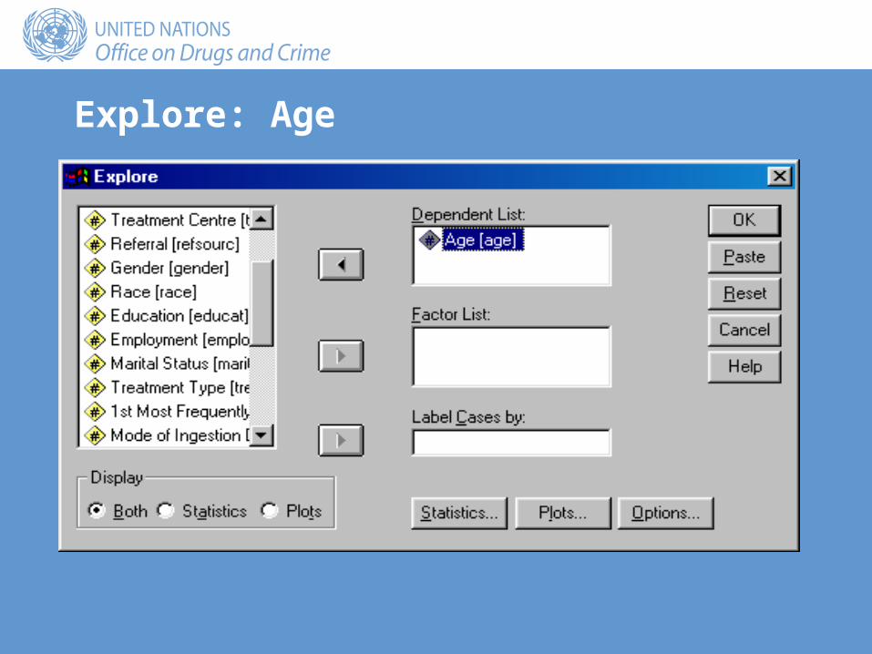
Explore: Age

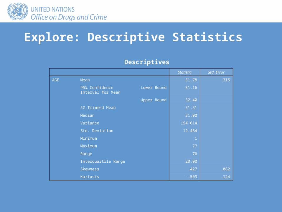
Explore: Descriptive Statistics

Statistic Std. Error

AGE Mean 31.78 .315

95% Confidence Interval for Mean

Lower Bound 31.16

Upper Bound 32.40

5% Trimmed Mean 31.31

Median 31.00

Variance 154.614

Std. Deviation 12.434

Minimum 1

Maximum 77

Range 76

Interquartile Range 20.00

Skewness .427 .062

Kurtosis -.503 .124

Descriptives

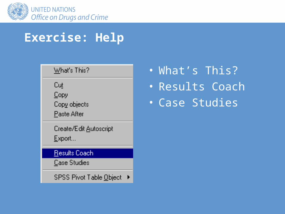
Exercise: Help

• What’s This?• Results Coach• Case Studies

Measures of central tendency

• Most commonly:– Mode– Median– Mean

• 5 per cent trimmed mean

The mode

• The mode is the most frequently occurring value in a dataset

• Suitable for nominal data and above• Example:

– The mode of the first most frequently used drug is Alcohol, with 717 cases, approximately 46 per cent of valid responses

Bimodal

• Describes a distribution• Two categories have a large number of cases• Example:

– The distribution of Employment is bimodal, employment and unemployment having a similar number of cases and more cases than the other categories

The median

• The middle value when the data are ordered from low to high is the median

• Half the data values lie below the median and half above

• The data have to be ordered so the median is not suitable for nominal data, but is suitable for ordinal levels of measurement and above

Example: median

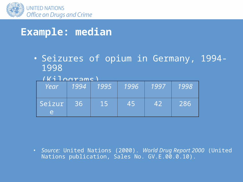
• Seizures of opium in Germany, 1994-1998(Kilograms)

• Source: United Nations (2000). World Drug Report 2000 (United Nations publication, Sales No. GV.E.00.0.10).

Year 1994 1995 1996 1997 1998

Seizure 36 15 45 42 286

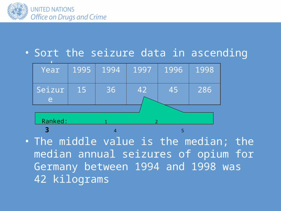
• Sort the seizure data in ascending order

• The middle value is the median; the median annual seizures of opium for Germany between 1994 and 1998 was 42 kilograms

Year 1995 1994 1997 1996 1998

Seizure 15 36 42 45 286

Ranked: 1 2 3 4 5

The mean

• Add the values in the data set and divide by the number of values

• The mean is only truly applicable to interval and ratio data, as it involves adding the variables

• It is sometimes applied to ordinal data or ordinal scales constructed from a number of Likert scales, but this requires the assumption that the difference between the values in the scale is the same, e.g. between 1 and 2 is the same as between 5 and 6

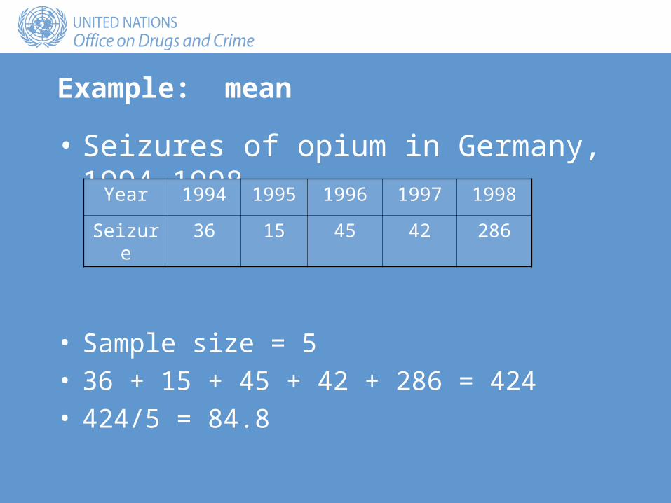
Example: mean

• Seizures of opium in Germany, 1994-1998

• Sample size = 5• 36 + 15 + 45 + 42 + 286 = 424• 424/5 = 84.8

Year 1994 1995 1996 1997 1998

Seizure 36 15 45 42 286

The 5 per cent trimmed mean

• The 5 per cent trimmed mean is the mean calculated on the data set with the top 5 per cent and bottom 5 per cent of values removed

• An estimator that is more resistant to outliers than the mean

95 per cent confidence interval for the mean

• An indication of the expected error (precision) when estimating the population mean with the sample mean

• In repeated sampling, the equation used to calculate the confidence interval around the sample mean will contain the population mean 95 times out of 100

Measures of dispersion

• The range• The inter-quartile range• The variance• The standard deviation

The range

• A measure of the spread of the data• Range = maximum – minimum

Quartiles

• 1st quartile: 25 per cent of the values lie below the value of the 1st quartile and 75 per cent above

• 2nd quartile: the median: 50 per cent of values below and 50 per cent of values above

• 3rd quartile: 75 per cent of values below and 25 per cent of the values above

Inter-quartile range

• IQR = 3rd Quartile – 1st Quartile• The inter-quartile range measures the spread or range

of the mid 50 per cent of the data • Ordinal level of measurement or above

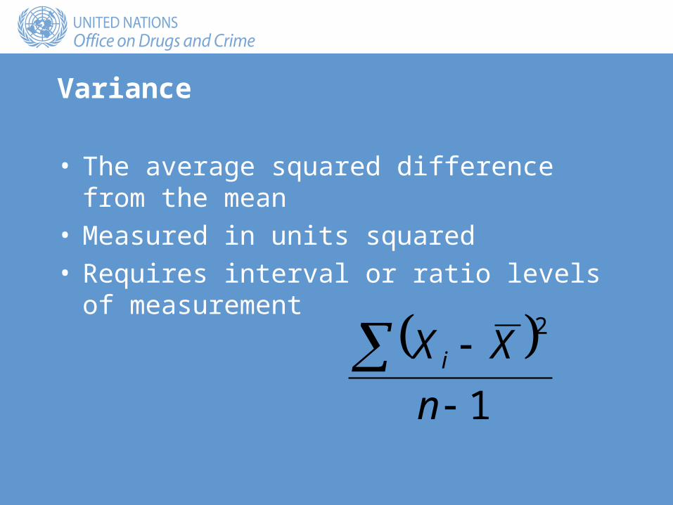
Variance

• The average squared difference from the mean• Measured in units squared• Requires interval or ratio levels of measurement

1

2

n

XX i

Standard deviation

• The square root of the variance• Returns the units to those of the original variable

1

2

n

XX i

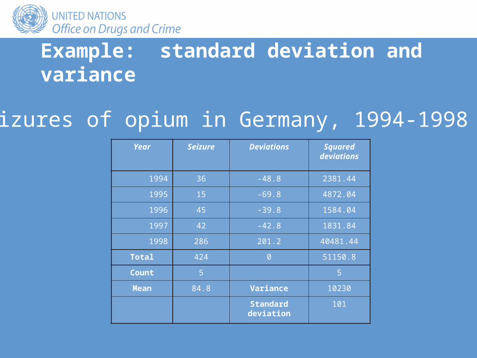
Example: standard deviation and variance

Seizures of opium in Germany, 1994-1998Year Seizure Deviations Squared

deviations

1994 36 -48.8 2381.44

1995 15 -69.8 4872.04

1996 45 -39.8 1584.04

1997 42 -42.8 1831.84

1998 286 201.2 40481.44

Total 424 0 51150.8

Count 5 5

Mean 84.8 Variance 10230

Standard deviation

101

Distribution or shape of the data

• The normal distribution• Skewness:

– Positive or right-hand skewed– Negative or left-hand skewed

• Kurtosis:– Platykurtic– Mesokurtic– Leptokurtic

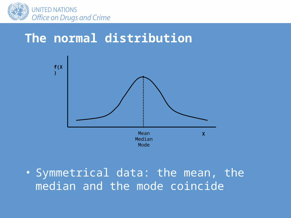
• Symmetrical data: the mean, the median and the mode coincide

MeanMedianMode

f(X)

X

The normal distribution

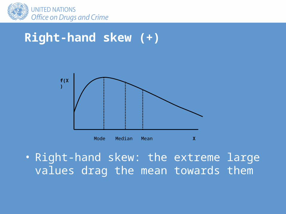
Right-hand skew (+)

• Right-hand skew: the extreme large values drag the mean towards them

f(X)

XMode Median Mean

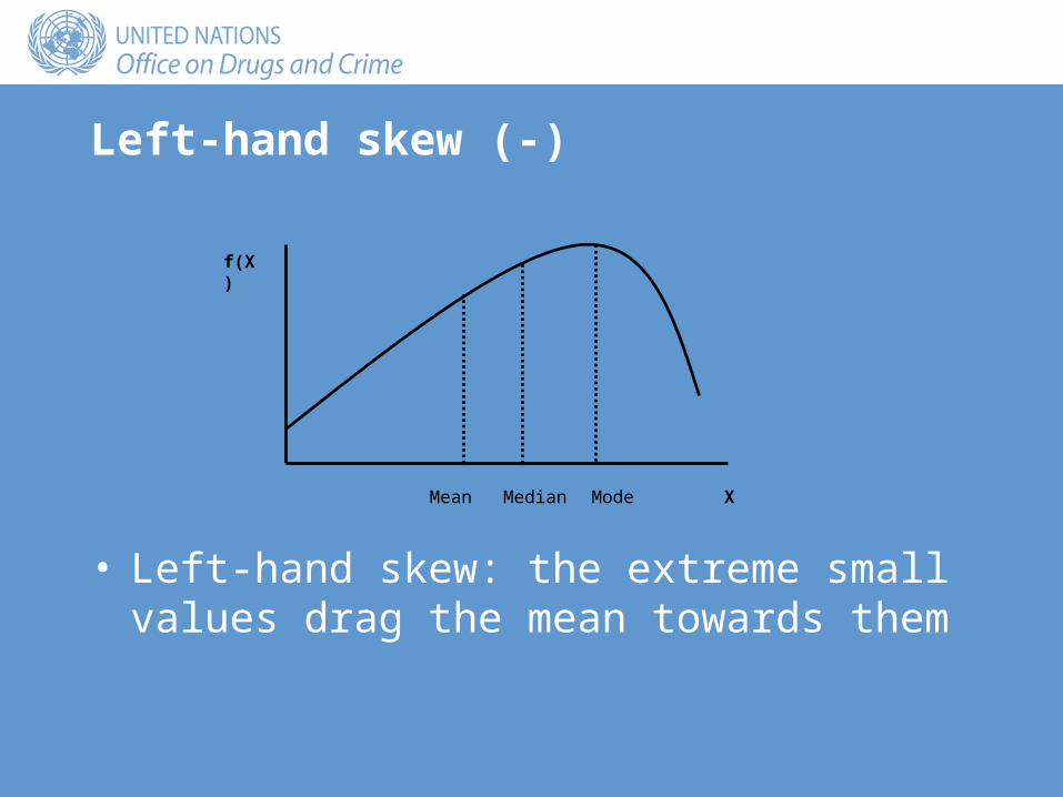
Left-hand skew (-)

• Left-hand skew: the extreme small values drag the mean towards them

ModeMean Median X

f(X)

Bivariate analysis

• Continuous Dependent Variable• Categorical Independent Variable

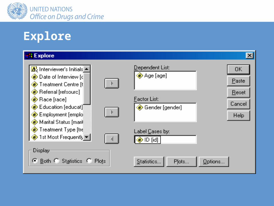
Explore

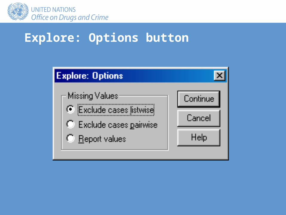
Explore: Options button

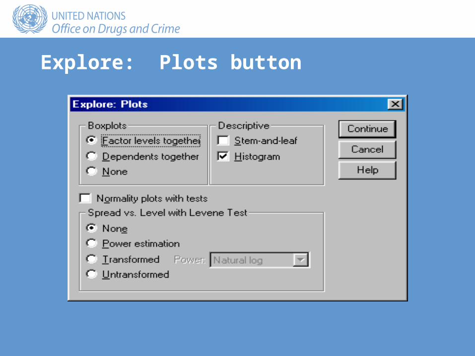
Explore: Plots button

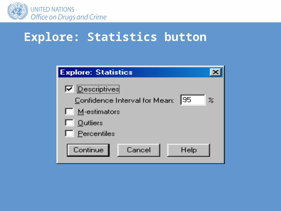
Explore: Statistics button

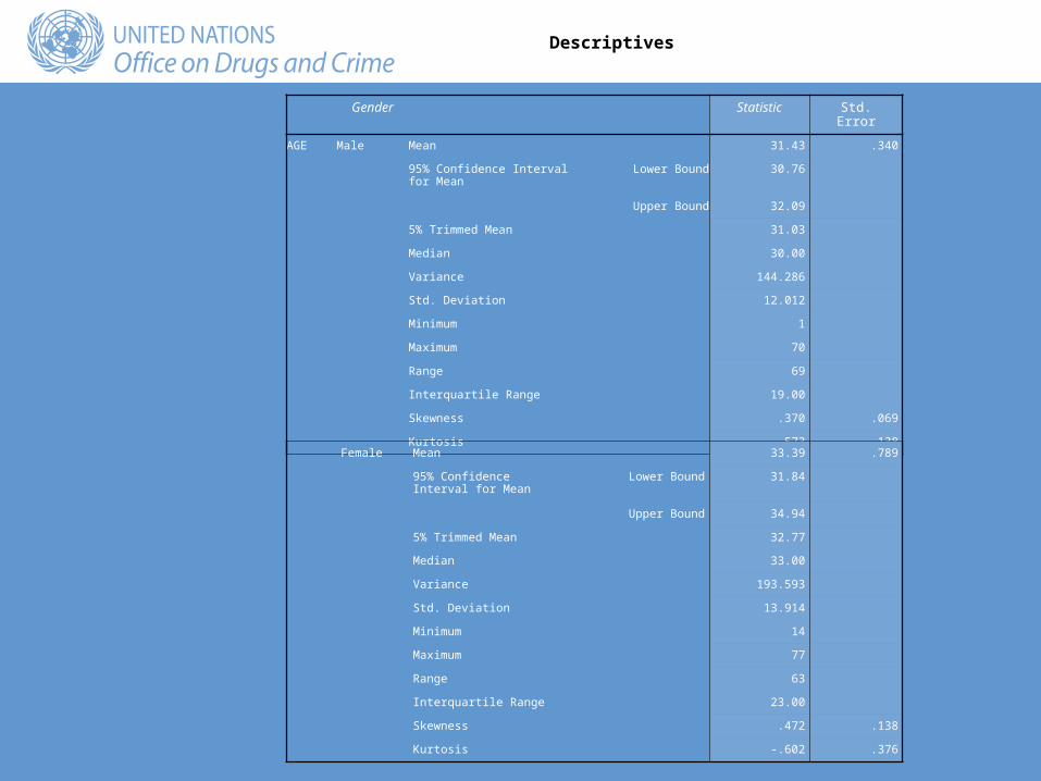
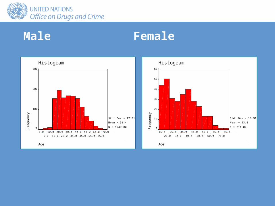
Gender Statistic Std. Error

AGE Male Mean 31.43 .340

95% Confidence Interval for Mean

Lower Bound 30.76

Upper Bound 32.09

5% Trimmed Mean 31.03

Median 30.00

Variance 144.286

Std. Deviation 12.012

Minimum 1

Maximum 70

Range 69

Interquartile Range 19.00

Skewness .370 .069

Kurtosis -.573 .138Female Mean 33.39 .789

95% Confidence Interval for Mean

Lower Bound 31.84

Upper Bound 34.94

5% Trimmed Mean 32.77

Median 33.00

Variance 193.593

Std. Deviation 13.914

Minimum 14

Maximum 77

Range 63

Interquartile Range 23.00

Skewness .472 .138

Kurtosis -.602 .376

Descriptives

Male Female

Age

70.0

65.0

60.0

55.0

50.0

45.0

40.0

35.0

30.0

25.0

20.0

15.0

10.0

5.0

0.0

Histogram

Fre

qu

en

cy

300

200

100

0

Std. Dev = 12.01

Mean = 31.4

N = 1247.00

Age

75.0

70.0

65.0

60.0

55.0

50.0

45.0

40.0

35.0

30.0

25.0

20.0

15.0

Histogram

Fre

qu

en

cy

60

50

40

30

20

10

0

Std. Dev = 13.91

Mean = 33.4

N = 311.00

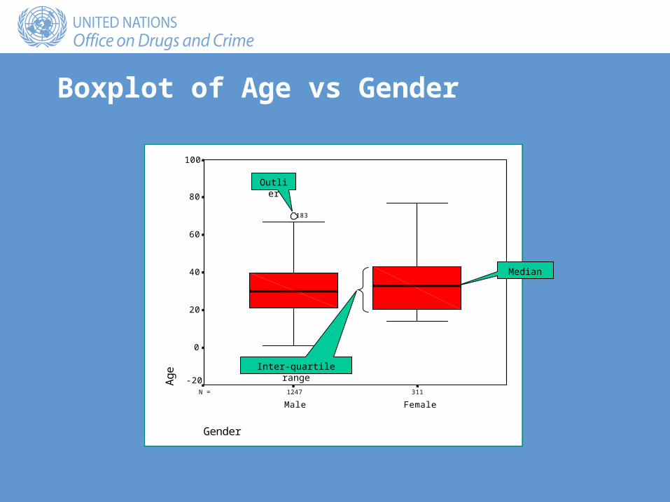
Boxplot of Age vs Gender

3111247N =

Gender

FemaleMale

Ag

e100

80

60

40

20

0

-20

183

Median

Inter-quartile range

Outlier

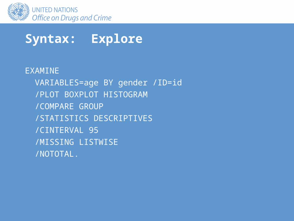
Syntax: Explore

EXAMINE

VARIABLES=age BY gender /ID=id

/PLOT BOXPLOT HISTOGRAM

/COMPARE GROUP

/STATISTICS DESCRIPTIVES

/CINTERVAL 95

/MISSING LISTWISE

/NOTOTAL.

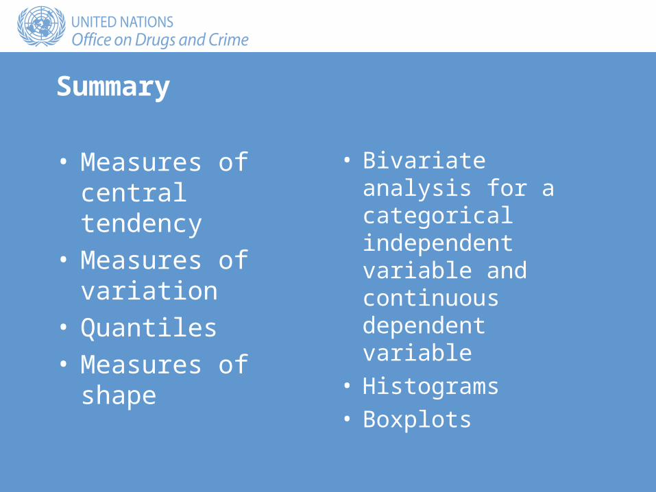
Summary

• Measures of central tendency

• Measures of variation• Quantiles• Measures of shape

• Bivariate analysis for a categorical independent variable and continuous dependent variable

• Histograms• Boxplots