DAPPLE: A Pipelined Data Parallel Approach forTraining Large Models

Shiqing Fan1, Yi Rong1, Chen Meng1, Zongyan Cao1, Siyu Wang1, Zhen Zheng1,Chuan Wu2, Guoping Long1, Jun Yang1, Lixue Xia1, Lansong Diao1, Xiaoyong Liu1, and Wei Lin1

1Alibaba Group, China2The University of Hong Kong, China

{shiqing.fsq, rongyi.ry, mc119496, zongyan.cao, siyu.wsy, james.zz}@alibaba-inc.comcwu@cs.hku.hk, {guopinglong.lgp, muzhuo.yj, lixue.xlx, lansong.dls, xiaoyong.liu, weilin.lw}@alibaba-inc.com

Abstract—It is a challenging task to train large DNN modelson sophisticated GPU platforms with diversified interconnectcapabilities. Recently, pipelined training has been proposed asan effective approach for improving device utilization. However,there are still several tricky issues to address: improving comput-ing efficiency while ensuring convergence, and reducing memoryusage without incurring additional computing costs. We proposeDAPPLE, a synchronous training framework which combinesdata parallelism and pipeline parallelism for large DNN models.It features a novel parallelization strategy planner to solve thepartition and placement problems, and explores the optimal hy-brid strategies of data and pipeline parallelism. We also proposea new runtime scheduling algorithm to reduce device memoryusage, which is orthogonal to re-computation approach and doesnot come at the expense of training throughput. Experimentsshow that DAPPLE planner consistently outperforms strategiesgenerated by PipeDreams planner by up to 3.23× speedupunder synchronous training scenarios, and DAPPLE runtimeoutperforms GPipe by 1.6× speedup of training throughput andsaves 12% of memory consumption at the same time.

Index Terms—deep learning, data parallelism, pipeline paral-lelism, hybrid parallelism

I. INTRODUCTION

The artificial intelligence research community has a longhistory of harnessing computing power to achieve significantbreakthroughs [1]. For deep learning, a trend has been increas-ing the model scale up to the limit of modern AI hardware.Many state-of-the-art DNN models (e.g., NLP [2], Internetscale E-commerce search/recommendation systems [3], [4])have billions of parameters, demanding tens to hundreds ofGBs of device memory for training. A critical challenge ishow to train such large DNN models on hardware accelerators,such as GPUs, with diversified interconnect capabilities.

A common approach is sychronous data parallel (DP) train-ing. Multiple workers each performs complete model compu-tation and synchronizes gradients periodically to ensure propermodel convergence. DP is simple to implement and friendlyin terms of load balance, but the gradients sychronizationoverhead can be a major factor preventing linear scalability.While the performance issue can be alleviated by optimizationssuch as local gradients accumulation [5]–[7] or computationand communication overlap techniques [8], [9], aggressiveDP typically requires large training batch sizes, which makesmodel tuning harder. More importantly, DP is not feasible once

the parameter scale of the model exceeds the memory limit ofa single device.

Recently, pipeline parallelism [10]–[12] has been proposedas a promising approach for training large DNN models.The idea is to partition model layers into multiple groups(stages) and place them on a set of inter-connected devices.During training, each input batch is further divided intomultiple micro-batches, which are scheduled to run overmultiple devices in a pipelined manner. Prior research onpipeline training generally falls into two categories. One ison optimizing pipeline parallelism for synchronous training[10], [11]. This approach requires necessary gradients syn-chronizations between adjacent training iterations to ensureconvergence. At runtime, it schedules as many concurrent pipestages as possible in order to maximize device utilization.In practice, this scheduling policy can incur notable peakmemory consumption. To remedy this issue, re-computation[13] can be introduced to trade redundant computation costsfor reduced memory usage. Re-computation works by check-pointing nodes in the computation graph defined by usermodel, and re-computing the parts of the graph in betweenthose nodes during backpropagation. The other category isasynchronous(async) pipeline training [12]. This manner in-serts mini-batches into pipeline continuously and discards theoriginal sync operations to achieve maximum throughput.

Although these efforts have made good contributions toadvance pipelined training techniques, they have some se-rious limitations. While PipeDream [14] made progress inimproving the time-to-accuracy for some benchmarks withasync pipeline parallelism, async training is not a commonpractice in important industry application domains due toconvergence concerns. This is reflected in a characterizationstudy [15] of widely diversified and fast evolving workloads inindustry scale clusters. In addition, the async approach requiresthe storage of multiple versions of model parameters. This,while friendly for increasing parallelism, further exacerbatesthe already critical memory consumption issue. As for syn-chronous training, current approach [10] still requires notablememory consumption, because no backward processing(BW)can be scheduled until the forward processing(FW) of allmicro-batches is finished. The intermediate results of somemicro-batches in FW need to be stored in the memory (for

arX

iv:2

007.

0104

5v1

[cs

.DC

] 2

Jul

202

0

corresponding BW’s usage later) while the devices are busywith FW of some other micro-batches. GPipe [10] proposesto discard some intermediate results to free the memory andre-computes them during BW when needed. But this mayintroduce additional ∼ 20% re-computation overhead [16].

In this paper, we propose DAPPLE, a distributed trainingscheme which combines pipeline parallelism and data par-allelism to ensure both training convergence and memoryefficiency. DAPPLE adopts synchronous training to guaranteeconvergence, while avoiding the storage of multiple versionsof parameters in async approach. Specifically, we addresstwo design challenges. The first challenge is how to deter-mine an optimal parallelization strategy given model structureand hardware configurations. The optimal strategy refers tothe one where the execution time of a single global steptheoretically reaches the minimum for given resources. Thetarget optimization space includes DP, pipelined parallelism,and hybrid approaches combining both. Current state-of-the-art pipeline partitioning algorithm [12] is not able to beapplied to synchronous training effectively. Some other work[10], [16] relies on empirical and manual optimizations, andstill lacks consideration of some parallelism dimensions. Weintroduce a synchronous pipeline planner, which generatesoptimal parallelization strategies automatically by minimizingexecution time of training iterations. Our planner combinespipeline and data parallelism (via stage-level replication) to-gether while partitioning layers into multiple stages. Besidespipeline planning, for those models that can fit into a singledevice and with high computation/communication ratio, theplanner is also capable of producing DP strategies directlyfor runtime execution. Furthermore, the planner takes bothmemory usage and interconnect topology constraints intoconsideration when assigning pipeline stages to devices. Theassignment of computation tasks to devices is critical fordistributed training performance in hardware environmentswith complex interconnect configurations. In DAPPLE, threetopology-aware device assignment mechanisms are definedand incorporated into the pipeline partitioning algorithm.

The second challenge is how to schedule pipeline stagecomputations, in order to achieve a balance among paral-lelism, memory consumption and execution efficiency. Weintroduce DAPPLE schedule, a novel pipeline stage schedulingalgorithm which achieves decent execution efficiency withreasonably low peak memory consumption. A key feature ofour algorithm is to schedule forward and backward stages ina deterministic and interleaved manner to release the memoryof each pipeline task as early as possible.

We evaluate DAPPLE on three representative applicationdomains, namely image classification, machine translation andlanguage modeling. For all benchmarks, experiments show thatour planner can consistently produce optimal hybrid paral-lelization strategies combining data and pipeline parallelismon three typical GPU hardware environments in industry, i.e.hierarchical NVLink + Ethernet, 25 Gbps and 10 Gbps Ether-net interconnects. Besides large models, DAPPLE also workswell for medium scale models with relatively large weights yet

small activations (i.e. VGG-19). Performance results show that(1) DAPPLE can find optimal hybrid parallelization strategyoutperforming the best DP baseline up to 2.32× speedup; (2)DAPPLE planner consistently outperforms strategies gener-ated by PipeDreams planner by up to 3.23× speedup undersynchronous training scenarios, and (3) DAPPLE runtimeoutperforms GPipe by 1.6× speedup of training throughputand reduces the memory consumption of 12% at the sametime.

The contributions of DAPPLE are summarized as follows:1) We systematically explore hybrid of data and pipeline

parallelism with a pipeline stage partition algorithm forsynchronous training, incorporating a topology-awaredevice assignment mechanism given model graphs andhardware configurations. This facilitates large modeltraining and reduces communication overhead of synctraining, which is friendly for model convergence.

2) We feature a novel parallelization strategy DAPPLEplanner to solve the partition and placement prob-lems and explore the optimal hybrid strategies of dataand pipeline parallelism, which consistently outperformsSOTA planner’s strategies under synchronous trainingscenarios.

3) We eliminate the need of storing multiple versions of pa-rameters, DAPPLE introduces a pipeline task schedulingapproach to further reduce memory consumption. Thismethod is orthogonal to re-computation approach anddoes not come at the expense of training throughput.Experiments show that DAPPLE can further save about20% of device memory on the basis of enabling re-computation optimization.

4) We provide a DAPPLE runtime which realizes efficientpipelined model training with above techniques withoutcompromising model convergence accuracy.

II. MOTIVATION AND DAPPLE OVERVIEW

We consider pipelines training only if DP optimizations [5],[6], [8], [17]–[20] are unable to achieve satisfactory efficiency,or the model size is too large to fit in a device with a minimumrequired batch size. In this section, we summarize key designissues in synchronous training with parallelism and motivateour work.

A. Synchronous Pipeline Training Efficiency

Pipeline training introduces explicit data dependencies be-tween consecutive stages (devices). A common approach tokeep all stages busy is to split the training batch into multiplemicro-batches [10]. These micro-batches are scheduled inthe pipelined manner to be executed on different devicesconcurrently.Note that activation communication (comm) over-head matters in synchronous training. Here we incorporatecomm as a special pipeline stage for our analysis. We definepipeline efficiency as average GPU utilization of all devicesin the pipeline. The pipeline efficiency is 1

1+P [10], where

P = (1+α)(S−1)M . S, M and α are number of stages, number of

equal micro-batches and communication-to-computation ratio,

respectively. Given a pipeline partitioning scheme (namelyfixed S and α), the larger the number of micro-batches M ,the higher the pipeline efficiency. Similarly, the smaller S, thehigher the efficiency for fixed α and M ,.

There are efforts to improve synchronous pipelines withmicro-batch scheduling [10], which suffer from two issues.

(1) Extra memory consumption. State-of-the-art approachinjects all micro-batches consecutively into the first stage ofFW. Then the computed activations are the input to BW.Execution states (i.e. activations) have to be kept in memoryfor all micro-batches until their corresponding BW operationsstart. Therefore, while more injected micro-batches may implyhigher efficiency, the memory limit throttles the number ofmicro-batches allowed.

(2) Redundant computations. State-of-the-art approach mayadopt activation re-computation to reduce peak memory con-sumption [13], i.e. discarding some activations during the FWphase, and recomputing them in the BW phase when needed.However, redundant computations come with extra costs. It isreported that re-computation can consume approximately 20%more execution time [16].

B. Pipeline Planning

To maximize resource utilization and training throughputfor pipelined training, it is crucial to find a good strategy forpartitioning stages and mapping stages to devices. We refer tothe stage partitioning and device mapping problem as pipelineplanning problem. Current state-of-the-art planning algorithm[14] may suffer from the following issues.

First, it does not consider synchronous pipeline training.Synchronous pipeline is very important as convergence isthe prerequisite of training. Compared against async pipelinetraining, an additional step is needed for sync pipeline trainingat the end of all micro-batches to synchronize parameterupdates. In more generic case where a stage may be replicatedon multiple devices, there exists additional gradients syn-chronizations (AllReduce) overheads before parameter updates.Current pipeline planner does not take such overhead intoconsideration and thus can not accurately model the end-to-end pipeline training time.

Second, previous approach does not consider the impact ofthe number of stages S, which is important for synchronousplanning. As discussed in the previous subsection, with fixedmicro-batches M and comm overhead ratio α, the fewer thenumber of stages(S) , the higher the pipeline efficiency.

Finally, uneven stage partitions have not been well studiedin existing works. We show in Section IV that uneven stagepartitions can sometimes produce better training performance.

C. The DAPPLE Approach

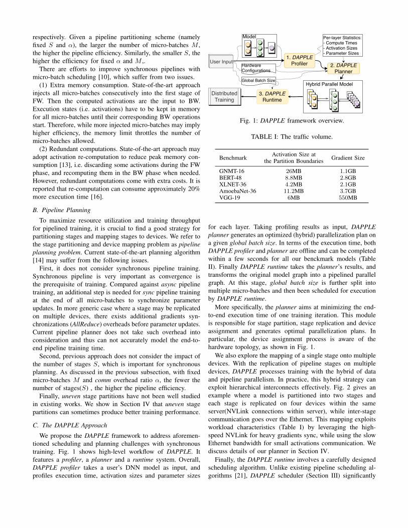
We propose the DAPPLE framework to address aforemen-tioned scheduling and planning challenges with synchronoustraining. Fig. 1 shows high-level workflow of DAPPLE. Itfeatures a profiler, a planner and a runtime system. Overall,DAPPLE profiler takes a user’s DNN model as input, andprofiles execution time, activation sizes and parameter sizes

2. DAPPLEPlanner

User Input1. DAPPLE

Profiler

Per-layer Statistics:- Compute Times- Activation Sizes- Parameter Sizes

DistributedTraining

3. DAPPLERuntime

HardwareConfigurations

Hybrid Parallel Model

Model

Global Batch Size

Fig. 1: DAPPLE framework overview.

TABLE I: The traffic volume.

Benchmark Activation Size atthe Partition Boundaries Gradient Size

GNMT-16 26MB 1.1GBBERT-48 8.8MB 2.8GBXLNET-36 4.2MB 2.1GBAmoebaNet-36 11.2MB 3.7GBVGG-19 6MB 550MB

for each layer. Taking profiling results as input, DAPPLEplanner generates an optimized (hybrid) parallelization plan ona given global batch size. In terms of the execution time, bothDAPPLE profiler and planner are offline and can be completedwithin a few seconds for all our benckmark models (TableII). Finally DAPPLE runtime takes the planner’s results, andtransforms the original model graph into a pipelined parallelgraph. At this stage, global batch size is further split intomultiple micro-batches and then been scheduled for executionby DAPPLE runtime.

More specifically, the planner aims at minimizing the end-to-end execution time of one training iteration. This moduleis responsible for stage partition, stage replication and deviceassignment and generates optimal parallelization plans. Inparticular, the device assignment process is aware of thehardware topology, as shown in Fig. 1.

We also explore the mapping of a single stage onto multipledevices. With the replication of pipeline stages on multipledevices, DAPPLE processes training with the hybrid of dataand pipeline parallelism. In practice, this hybrid strategy canexploit hierarchical interconnects effectively. Fig. 2 gives anexample where a model is partitioned into two stages andeach stage is replicated on four devices within the sameserver(NVLink connections within server), while inter-stagecommunication goes over the Ethernet. This mapping exploitsworkload characteristics (Table I) by leveraging the high-speed NVLink for heavy gradients sync, while using the slowEthernet bandwidth for small activations communication. Wediscuss details of our planner in Section IV.

Finally, the DAPPLE runtime involves a carefully designedscheduling algorithm. Unlike existing pipeline scheduling al-gorithms [21], DAPPLE scheduler (Section III) significantly

GPU0

GPU1

GPU2

GPU3

GPU0

GPU1

GPU2

GPU3

NVLink

Ethernet

PipelineParallelism

Machine0(Stage0) Machine1(Stage1)DataParallelism

NVLink

NVLink

NVLink

NVLink

NVLink

Fig. 2: Device mapping on hierarchical interconnects.

reduces the need for re-computation, retains a reasonable levelof memory consumption, while saturates the pipeline withenough micro-batches to keep all devices busy.

III. DAPPLE SCHEDULE

A. Limitations of GPipe ScheduleTo improve pipeline training efficiency, GPipe [10] proposes

to split global batch into multiple micro-batches and injectsthem into the pipeline concurrently (Fig. 3 (a)). However,this scheduling pattern alone is not memory-friendly and willnot scale well with large batch. The activations producedby forward tasks have to be kept for all micro-batches untilcorresponding backward tasks start, thus leads to the mem-ory demand to be proportional (O(M)) to the number ofconcurrently scheduled micro-batches (M ). GPipe adopts re-computation to save memory while brings approximately 20%extra computation. In DAPPLE, we propose early backwardscheduling to reduce memory consumptions while achievinggood pipeline training efficiency(Fig. 3 (b)).

B. Early backward schedulingThe main idea is to schedule backward tasks(BW) earlier

and hence free the memory used for storing activations pro-duced by corresponding forward tasks(FW). Fig. 3(b) showsDAPPLE’s scheduling mechanism, compared to GPipe in Fig.3 (a). Firstly, instead of injecting all M micro-batches atonce, we propose to inject K micro-batches (K < M ) atthe beginning to release memory pressure while retaining highpipeline efficiency. Secondly, we schedule one FW of a micro-batch followed by one BW strictly to guarantee that BWcan be scheduled earlier. Fig. 3 (c) shows how the memoryconsumptions change over time in GPipe and DAPPLE. Atthe beginning, the memory usage in DAPPLE increases withtime and is the same as GPipe’s until K micro-batches areinjected, then it reaches the maximum due to the early BWscheduling. Specifically, with strictly controlling the executionorder of FW and BW, the occupied memory for activationsproduced by the FW of a micro-batch will be freed afterthe corresponding BW so that it can be reused by the nextinjected micro-batch. In comparison, GPipe’s peak memoryconsumptions increases continuously and has no opportunityfor early release. Moreover, DAPPLE does not sacrifice inpipeline training efficiency. Actually, DAPPLE introduces the

6Forward Backward

GPU0

GPU1

GPU2

GPU0

GPU1

GPU2

00

0

11

1

223

23

3 33

3

22

2

11

1

00

0

45

56

6

4 54

66

6

554

445

PeakMem

ory

Time

200

0

11

1 2

332

3 33

3

22

2

11

1

00

0 44

4

55

5

66

644

4

55

5

66

6

(c)MemoryconsumptionofGPU0from(a)and(b)

(a)GPipe(b)DAPPLE

(b)DAPPLE

(a)GPipe

Fig. 3: The different scheduling between GPipe(a) and DAP-PLE(b) and their memory consumptions.

1

0 1

0 1 2 3

0

0

4

Stage4AllReduce

Stage0

Stage1

Forward Backward

2

0 1 2

0 1 2

0

0 1

1 1

0

0

0

0

3

3

3

2

2 2

2

3

3

3

3

1

1

1

4

4

4

2

2

2

5 1 6 2 7 3

5

5

5

3

3

3 6

6

6 4

4

4 7

7

7

4

4 4

4

5

5

5

5

6

6 6

6

7

7 7

7

5

5

5

6

6

6

7

7

7

4 5 6 7

Stage2AllReduce

AllReduce NetworkTransmission

Stage2

Tw (Warmup Phase) Ts (Steady Phase) Te (Ending Phase)

Stage3

Stage4

Bubble

Fig. 4: DAPPLE pipeline example.

exact same bubble time as GPipe when given the same stagepartition, micro-batches and device mapping. We will presentthe details in section V-C.

Note that the combination of early backward scheduling andre-combination allows further exploitation in memory usage.We present performance comparisons of DAPPLE and GPipein section VI-D.

IV. DAPPLE PLANNERDAPPLE Planner generates an optimal hybrid parallelism

execution plan given profiling results of DAPPLE profiler,hardware configurations and a global training batch size.

A. The Optimization ObjectiveFor synchronous training, we use the execution time of a

single global batch as our performance metric, which we callpipeline latency. The optimization objective is to minimizepipeline latency L with the consideration of all solution spacesof data/pipeline parallelism.

In synchronous pipelined training, computations and cross-stage communication of all stages usually form a trapezoid,but not diamond formed by normal pipelines without backwardphase. Fig.4 shows a pipelined training example with welldesigned task scheduling arrangement. We use blue blocksfor forward computation, and green ones for backwards, withnumbers in them being the corresponding micro-batch index.Network communications are arranged as individual stages.Gray blocks are bubbles.

We denote the stage with the least bubble overhead as pivotstage, which will be the dominant factor in calculating pipelinelatency L. Let its stage id be Q. We will discuss about howto choose pivot stage later.

A pipeline training iteration consists of warmup phase,steady phase and ending phase, as shown in Fig. 4 in whichpivot stage is the last stage. Pivot stage dominates steadyphase. We call the execution period from the start to pivotstage’s first micro-batch as warmup phase in a pipeline iter-ation, the period from pivot stage’s last micro-batch to theend as ending phase. Pipeline latency is the sum of thesethree phases. The optimization objective for estimating L isas follows:

Tw =

Q∑s=0

Fs

Ts = (M − 1)× (FQ +BQ)

Te =S−1maxs=0

(AR(Ps, gs) +

{−∑sa=QBa s ≥ Q∑Q

a=sBa s < Q)

(1)

L = Tw + Ts + Te (2)

Tw denotes the execution time of warmup phase, which isthe sum of forward execution time of stages till Q for onemicro-batch. Ts denotes the steady phase, which includes bothforward and backward time of stage Q for all micro-batchesexcept for the one contributing to warmup and ending phase.Te corresponds to the ending phase. Te includes allreduceoverhead and thus considers stages both before and after Q.Note that some stages before Q may contribute to Te withallreduce cost. M , S, Fs and Bs denote the total number ofmicro-batches, the number of stages (computation stages +network stages), forward and backward computation time ofstage s, respectively. AR(Ps, gs) represents the gradients syn-chronization (AllReduce) time for stage s, with its parameterset Ps on the device set gs.

Note we consider inter-stage communication as an indepen-dent stage alongside the computation stages. The AllReducetime AR(Ps, gs) is always 0 for communication stages. More-over, we define Fs and Bs for a communication stages as itsfollowing forward and backward communication time.

In practice, synchronous pipelines in some cases includebubbles in stage Q, which may contribute a small fractionof additional delay to time. This objective does not modelthose internal bubbles, and thus is an approximation to thetrue pipeline latency. But it works practically very well for allour benchmarks (Section VI).

B. Device AssignmentDevice assignment affects communication efficiency and

computing resource utilization. Previous work [12] uses hi-erarchical planning and works well for asynchronous training.However, it lacks consideration of synchronous pipeline train-ing, in which the latency of the whole pipeline, rather than of asingle stage, matters to overall performance. It cannot be used

OccupiedGPUi ReturnedGPUiafterpolicy AvailableGPUi

10 32 54 76

98 1110 1312 1514

10 32 54 76

98 1110 1312 1514

1716 1918 2120 2322

10 32 54 76

98 1110 1312 1514

1716 1918 2120 2322

(c)AppendFirstbasedon(a)

(b)FreshFirstbasedon(a)

(d)ScatterFirstbasedon(a)

M2

M1

M0

i i i

(a)Originaldeviceassignmentstate

1716 1918 2120 2322

10 32 54 76

98 1110 1312 1514

1716 1918 2120 2322

M2

M1

M0

Mk: the kth machine

Fig. 5: Device assignment examples: applying for 6 devicesusing three different strategies respectively from (a).

to efficiently estimate the whole pipeline latency. Meanwhile,it does not allow stages to be placed on arbitrary devices.Our approach essentially allows a specific stage to be mappedto any set of devices, and therefore is able to handle moreplacement cases, at a reasonable searching cost.

Instead of enumerating all possibilities of placement plansusing brute force, we designed three policies (Fig. 5), andexplore their compositions to form the final placement plan.

a) Fresh First: allocate GPUs from a fresh machine. Ittends to put tasks within a stage onto the same machine,which can leverage high-speed NVLink [22] for intra-stagecommunication. A problem of this policy is that, it can causefragmentation if the stage cannot fully occupy the machine.

b) Append First: allocate from machines that alreadyhave GPUs occupied. It helps to reduce fragmentation. It alsolargely implies that the stage is likely to be within the samemachine.

c) Scatter First: try to use available GPUs equally fromall used machines, or use GPUs equally from all machinesif they are all fresh. It is suitable for those stages that havenegligible weights compared to activation sizes (less intra-stage communication). This policy could also serve as an in-termediate state to allocate GPU with minimal fragmentation.

The overall device placement policies reduce search spaceeffectively down to less than O(2S), while retaining room forpotential performance gain.

C. Planning AlgorithmOur planning algorithm use Dynamic Programming to find

the optimal partition, replication and placement strategy, sothat the pipeline latency L is minimized. Here we first presenthow to update the pivot stage ID Q along the planning process,and then the formulation of our algorithm

1) Determining The Pivot Stage Q: It is vital to select aproper pivot stage Q for the estimation of L. The insight is tofind the stage with minimum bubbles, which dominates steadyphase. We use a heuristic to determine Q (formula 3).

Q = arg0

maxs=S−1

max(TQst +

Q−1∑s′=s+1

(Fs′ +Bs′), Tsst

)(3)

The initial Q is set to S−1. DAPPLE updates Q iterativelyfrom stage S − 1 to stage 0 according to formula 3. T jst =(M − 1) × (Fj + Bj) means the duration of steady phase,

Plannedlayers Newstages'1

mGPUs m'GPUs

0 j j' N-1

Newstages'2

layerid:Currently, we get:TPL(j, m, g)

Next step, we get:TPL(j', m+m', g+g')

(G-m-m')GPUs

Fig. 6: Planning process for j’.

without bubbles, suppose pivot stage is j. For a stage s <Q, if T sst is larger than the sum of TQst and correspondingforward/backward costs between s and current Q, it meansthe steady phase will have less bubbles if pivot stage is set ass other than current Q. Q will then be updated to s.

2) Algorithm Formulation: We define the estimatedpipeline latency TPL(j,m, g) as the subproblem, for whichwe have planned the strategy for the first j layers using mGPUs (with device id set g). The unplanned layers forms thelast stage and replicates on the other (G − m) GPUs. Ourobjective is to solve for TPL(N,G,G),G = {0, 1, ..., G− 1}.N , G and G denote the number of layers, number of GPUsand GPU set, respectively. Formula 4 describes the algorithm.

TPL(N,G,G) = min1≤j<N

min1≤m<G

ming∈D(G,m)

TPL(j,m, g) (4)

Fig. 6 describes the iterative planning process. Suppose wehave already planned for the first j (0 ≤ j < N ) layersand have the estimation TPL(j,m, g) as pipeline latency. Thelayers after j forms a stage s′. Meanwhile, we get the optimalQ for current strategy along with the cost of FQ and BQfor stage Q. Next step, we try to add one more partition instage s′, supposing after layer j′ (j < j′ ≤ N ), and split s′

into two new stages s′1 and s′2. We assign m′ GPUs for s′1 and(G−m−m′) GPUs for s′2, and estimate TPL(j′,m+m′, g+g′)according to formula 5. Note DAPPLE enumerates the threestrategies in section IV-B for device placement of stage s′1.

TPL(j′,m+m′, g + g′) = L (5)

Here, L is the same with that in formula 2. The key forthe estimation of L in formula 5 is to find Q of subproblemTPL(j

′,m+m′, g+g′). In the sample in Fig. 6, we get Qj forTPL(j,m, g). We apply formula 3 to get Qj′ for TPL(j,m+m′, g + g′) with the help of Qj : if Qj is not s′, we do notneed to iterate all stages before j, but use Qj for all stagesbefore layer j instead in the iterative process.

Along the above process, we record the current best split,replication and placement for each point in our solution spaceusing memorized search.

D. Contributions over previous workPrevious works on pipeline planning includes PipeDream

[12] (for asynchronous training) and torchgpipe [23], a com-munity implementation of GPipe [10] which uses “Block Par-titioning of Sequences” [24]. Both aim to balance the workloadacross all GPUs. While this idea works good in PipeDream’sasynchronous scenarios and gives reasonable solutions under

ForwardBackward

GPU0

GPU10

00

GPU0GPU1

10 0 1

01

1

10

01 1

1

Fig. 7: Uneven pipeline minimum example.

GPipe’s synchronous pipeline for its micro-batch arrangement,we found that our micro-batch arrangement could achieveeven higher performance by 1) intentionally preferring slightlyuneven partitioning with fewer stages, and 2) exploring abroader solution space of device assignment. The followingsections highlight our contributions of planning for hybridparallelism. The resulting strategies and performance gain onreal-world models will be demonstrated in Section VI-F.

1) Uneven Pipeline Partitioning with Fewer Stages: In syn-chronous Pipeline Parallelism scenarios, we found two insightsthat could provide an additional performance improvements.The first one is to partition the model into as few stagesas possible to minimize the bubble overhead under the samenumber of micro-batches. This conclusion is also mentionedin GPipe. The second one is that partitioning the model in aslightly uneven way yields much higher performance than aperfectly even split, like the example in Fig. 7.

2) Versatile Device Placement: DAPPLE device assign-ment strategy covers a broad solution space for stage place-ment, and is a strict superset of PipeDream’s hierarchical re-cursive partitioning approach. This allows us to handle variousreal world models. For example, for models that have layerswith huge activations compared to their weights, DAPPLEallows such a layer to be replicated across multiple machines(Scatter First) to utilize high-speed NVLink for activationcommunication and low-speed Ethernet for AllReduce.

V. DAPPLE RUNTIME

A. Overview

We design and implement DAPPLE runtime in Tensorflow[25] (TF) 1.12, which employs a graph based executionparadigm. As common practices, TF takes a precise andcomplete computation graph (DAG), schedules and executesgraph nodes respecting all data/control dependencies.

DAPPLE runtime takes a user model and its planning resultsas input, transforms the model graph into a pipelined parallelgraph and executes on multiple distributed devices. It firstbuilds forward/backward graphs separately for each pipe stage.Then additional split/concat nodes are introduced between ad-jacent stages for activation communication. Finally, it builds asubgraph to perform weights update for synchronous training.This step is replication aware, meaning it will generate dif-ferent graphs with or without device replication of stages. Weleverage control dependences in TF to enforce extra executionorders among forward/backward stage computations. SectionV-B presents how to build basic TF graph units for a singlemicro-batch. Section V-C discusses how to chain multiplesuch units using control dependencies to facilitate DAPPLEexecution.

(a)Splitreplicatedstageacrossmultipledevicesbydividingmicrobatchsize

(b)Eachdeviceofreplicatedstageconsumesthewholemicrobatchsizeandresultinginmorebubbles

GPU2

GPU1

GPU0Stage0

Stage1

0 0 1 1 2 2 3 3 4 41 3 1 30 2 0 4 2 4

GPU2GPU1

GPU0Stage0

Stage1

Forward

Backward

Idle

0 0 1 1 2 2 3 3 4 40 1 0 2 1 3 2 4 3 40 1 0 2 1 3 2 4 3 4

Fig. 8: Efficiency of two stage replication approaches. Stage0 consumes twice as much time as stage 1 for a micro-batch.

B. Building Micro-batch Units

1) Forward/Backward Stages: In order to enforce executionorders with control dependencies between stages, we need tobuild forward and backward graphs stage by stage to deal withthe boundary output tensors such as activations.

Specifically, we first construct the forward graph of eachstage in sequence and record the boundary tensors. No back-ward graphs should be built until all forward graphs are ready.Second, backward graphs will be built in reverse order for eachstage.

2) Cross Stage Communication: DAPPLE replicates somestages such that the number of nodes running a stage canbe different between adjacent stages, and the communicationpatterns between them are different from straight pipelinedesign. We introduce special split-concat operations betweenthese stages.

Fig. 8(a) shows the replication in DAPPLE for a 2-stagepipeline, whose first stage consumes twice as much time asthe second stage for a micro-batch and thus is replicated ontwo devices. For the first stage, we split the micro-batch furtherinto 2 even slices, and assign each to a device. An alternativeapproach [12] (Fig. 8(b)) is not to split, but to schedule anentire micro-batch to two devices in round robin manner.However, the second approach has lower pipeline efficiencydue to tail effect [26]. Though the second approach does notinvolve extra split-concat operations, the overhead of tail effectis larger than split-concat in practice. We hence use the firstapproach with large enough micro-batch size setting to ensuredevice efficiency.

The split-concat operations include one-to-many, many-to-one and many-to-many communication. We need split forone-to-many(Fig. 9(b)), that is, splitting the micro-batch intoeven slices and sending each slice to a device in the nextstage. We need concat for many-to-one(Fig. 9(c)), where allslices should be concatenated from the previous stage and fedinto the device in the next stage. For many-to-many(Fig. 9(d))we need both split and concat of micro-batch slices toconnect adjacent stages. If two adjacent stages have the samereplication count, no split-concat is needed.

3) Synchronous Weights Update: Weights updating in DAP-PLE is different with naive training as there are multiplemicro-batches injected concurrently. Meanwhile, the replica-tion makes weights updating more complex. As is shown in

0 1 1 0(a)Noreplication

01

1

1

10S C

10

0

0

01 SC

10

0

0

01

S1

1

1

1

CS

SC

C

(b)Onetomany

(c)Manytoone

(d)ManytomanyS Split Node C Concat Node Forward Pass Backward Pass

Fig. 9: Split-Concat for Cross Stage Communication

GA Apply

Apply

AllR

educe

Replica0

reducedgradients

reducedgradientsReplican

......

accumulatedgradients

computenextmicrobatch

GA

accumulatedgradients

gradientsFW BW

BWFWgradients

computenextmicrobatch

Fig. 10: Weights update. GA means gradient accumulation [5].

Fig. 10, each device produces and accumulates gradients forall micro-batches. There is an AllReduce operation to synchro-nize gradients among all replicas, if exists. A normal Applyoperation updates weights with averaged gradients eventually.

C. Micro-batch Unit Scheduling

The early backward scheduling strikes a trade-off betweenmicro-batch level parallelism and peak memory consumption:feeding more micro-batches into pipeline at once implieshigher parallelism, but may lead to more memory usage.

DAPPLE scheduler enforces special execution orders be-tween micro-batches to reduce memory usage. For the firststage, we suppose K micro-batches are scheduled concurrentlyat the beginning for forward computation. Specifically, Ki isthe number of scheduled micro-batches at the beginning forstage i. The overall execution follows a round robin order withinterleaving FW and BW.

We realize the scheduler with control dependency edges inTF. Fig. 11 shows how up to three micro-batches are connectedvia control dependencies to implement the schedule for a twostage pipeline. Control dependency is not necessary when thereis only one micro-batch (Fig. 11(a)). With two micro-batches(Fig. 11(b)), two control edges are introduced. The controledge between B0 and F1 in stage 1 is to form the roundrobin order of FW and BW. The early execution of B0 helpsto free memory of F0 and B0 in stage 1, which can bereused in following tasks. The edge between F0 and F1 in

F0GPU0

ForwardPass

BackwardPassB0F0

B0

F0

B0F0

B0F1

F1 B1

B1

F0

B0F0

B0F1

F1 B1

B1F2

F2 B2

B2

GPU1

(a)Onemicro-batch

(b)Twomicro-batches

(c)Threemicro-batches

DataDependency

ControlDependency

GPU0

GPU1

GPU0

GPU1

Fig. 11: Micro-batches scheduling. The solid blue and dottedred arrows denote data and control dependencies, respectively.

stage 0 is to enforce the order that micro-batch 1 is strictlyexecuted after micro-batch 0, thus the backward of micro-batch 0 can be executed earlier and its corresponding memorycan be freed earlier. In practice, F0 and F1 are typically largechunks of computations. The lack of parallelism between F0and F1 does not affect the gain of reducing memory usage.The situation with three micro-batches (Fig. 11(c)) is the same.

An appropriate Ki is essential as it indicates the peak mem-ory consumption for stage i. There are two primary factors fordeciding Ki: memory demand for one micro-batch execution,and the ratio between cross stage communication latency andthe average FW/BW computation time (referred as activationcommunication ratio, ACR in short). The former determineshow many forward batches can be scheduled concurrentlyat most. We define the maximum number of micro-batchessupported by the device memory as D; Lower ACR meansless warm up forward batches Ki (smaller Ki) are enough tosaturate the pipeline. While notable ACR means larger Ki isnecessary.

We implement two policies to set Ki in practice. Policy A(PA): Ki = min(S − i,D). PA works well when ACR issmall, i.e. the impact of cross stage communication overheadis negligible. Policy B (PB): Ki = min(2 ∗ (S − i) − 1, D).Here we schedule twice the number of forward micro-batchesthan PA. The underlying intuition is that in some workloads,the cross stage communication overhead is comparable withforward/backward computations and thus more micro-batchesis needed to saturate the pipeline.

VI. EVALUATION

A. Experimental Setup

Benchmarks. Table II summarizes all the six representativeDNN models that we use as benchmarks in this section. Thedatasets applied for the three tasks are WMT16 En-De [27],SQuAD2.0 [28] and ImageNet [29], respectively.

Hardware Configurations. Table III summarizes three com-mon hardware environments for DNN training in our exper-iments, where hierarchical and flat interconnections are bothcovered. In general, hierarchical interconnection is popular in

TABLE II: Benchmark models.

Task Model # ofParams

(cbch Size,Memory Cost)

Translation GNMT-16 [30] 291M (64, 3.9GB)LanguageModel

BERT-48 [31] 640M (2, 11.4GB)XLNet-36 [32] 500M (1, 12GB)

ImageClassification

ResNet-50 [33] 24.5M (128, 1GB)VGG-19 [34] 137M (32, 5.6GB)AmoebaNet-36 [35] 933M (1, 20GB)

TABLE III: Hardware configurations.

Config GPU(s) perserver(Ns)

Intra-serverconnnections

Inter-serverconnections

A 8x V100 NVLink 25 GbpsB 1x V100 N/A 25 GbpsC 1x V100 N/A 10 Gbps

industry GPU data centers. We also consider flat Ethernet net-works interconnections because NVLink may not be availableand GPU resources are highly fragmented in some real-worldproduction clusters. Specifically, Config-A (hierarchical) hasservers each with 8 V100 interconnected with NVLink, and a25Gbps Ethernet interface. Config-B (flat) has servers eachwith only one V100 (no NVLink) and a 25Gbps Ethernetinterface. Config-C (flat) is the same with Config-B exceptwith only 10 Gbps Ethernet equipped. The V100 GPU has16 GB of device memory. All servers run 64-bits CentOS 7.2with CUDA 9.0, cuDNN v7.3 and NCCL 2.4.2 [36].Batch Size and Training Setup. The batch sizes of offlineprofiling for the benchmarks are shown in the last columnof Table II (ch size. As for AmoebaNet-36, it reaches OOMeven if batch size = 1 on a single V100. Thus we extendto two V100s where batch size = 1 just works. We uselarge enough global batch size for each benchmark to ensurehigh utilization on each device. All global batch sizes we useare consistent with common practices of the ML community.We train GNMT-16, BERT-48 and XLNet-36 using the Adamoptimizer [37] with initial learning rate of 0.0001, 0.0001, 0.01and 0.00003 respectively. For VGG19, we use SGD with aninitial learning rate of 0.1. For AmoebaNet, we use RMSProp[38] optimizer with an initial learning rate of 2.56. We use fp32for training in all our experiments. Note that all the pipelinelatency optimizations proposed in this paper give equivalentgradients for training when keeping global batch size fixedand thus convergence is safely preserved.

B. Planning Results

Table V summarizes DAPPLE planning results of five mod-els in the three hardware environments, where the total numberof available devices are all fixed at 16. The first column alsogives the global batch size (GBS) correspondingly.

We use three notations to explain the output plans. (1) Aplan of P : Q indicates a two stage pipeline, with the firststage and the second stages replicated on P and Q devices,

0

4

8

12

16

0 1024 2048 3072 4096

Trai

ning

Spee

dup

Global Batch Size

DP No Overlap

DP+Normal Overlap

Best Hybrid Speedup

(a) VGG19 on config A

0

4

8

12

16

0 1024 2048 3072 4096

Trai

ning

Spee

dup

Global Batch Size

DP No Overlap

DP+Normal Overlap

Best Hybrid Speedup

(b) VGG19 on config B

0

4

8

12

16

0 1024 2048 3072 4096

Trai

ning

Spee

dup

Global Batch Size

DP No Overlap

DP+Normal Overlap

Best Hybrid Speedup

(c) VGG19 on config C

0

4

8

12

16

0 1024 2048 3072 4096

Trai

ning

Spee

dup

Global Batch Size

DP No Overlap

DP+Normal Overlap

Best Hybrid Speedup

(d) GNMT-16 on config A

0

4

8

12

16

0 1024 2048 3072 4096

Trai

ning

Spee

dup

Global Batch Size

DP No Overlap

DP+Normal Overlap

Best Hybrid Speedup

(e) GNMT-16 on config B

0

4

8

12

16

0 1024 2048 3072 4096

Trai

ning

Spee

dup

Global Batch Size

DP No Overlap

DP+Normal Overlap

Best Hybrid Speedup

(f) GNMT-16 on config C

0

4

8

12

16

0 64 128 192 256

Trai

ning

Spee

dup

Global Batch Size

DP No Overlap

DP+Normal Overlap

Best Hybrid Speedup

(g) BERT-48 on config A

0

4

8

12

16

0 64 128 192 256

Trai

ning

Spee

dup

Global Batch Size

DP No Overlap

DP+Normal Overlap

Best Hybrid Speedup

(h) BERT-48 on config B

0

4

8

12

16

0 64 128 192 256Tr

aini

ngSp

eedu

p

Global Batch Size

DP No Overlap

DP+Normal Overlap

Best Hybrid Speedup

(i) BERT-48 on config C

0

4

8

12

16

0 64 128 192 256

Trai

ning

Spee

dup

Global Batch Size

DP No Overlap

DP+Normal Overlap

Best Hybrid Speedup

(j) XLNet-36 on config A

0

4

8

12

16

0 64 128 192 256

Trai

ning

Spee

dup

Global Batch Size

DP No Overlap

DP+Normal Overlap

Best Hybrid Speedup

(k) XLNet-36 on config B

0

4

8

12

16

0 64 128 192 256

Trai

ning

Spee

dup

Global Batch Size

DP No OverlapDP+Normal OverlapBest Hybrid Speedup

(l) XLNet-36 on config C

0

4

8

12

16

0 256 512 768 1024

Trai

ning

Spee

dup

Global Batch Size

DP No Overlap

DP+Normal Overlap

Best Hybrid Speedup

(m) AmoebaNet-36 on config A

0

4

8

12

16

0 256 512 768 1024

Trai

ning

Spee

dup

Global Batch Size

DP No Overlap

DP+Normal Overlap

Best Hybrid Speedup

(n) AmoebaNet-36 on config B

0

4

8

12

16

0 256 512 768 1024

Trai

ning

Spee

dup

Global Batch Size

DP No Overlap

DP+Normal Overlap

Best Hybrid Speedup

(o) AmoebaNet-36 on config C

Fig. 12: Speedups on configurations with hierarchical/flat interconnects.

TABLE IV: Normalized training throughput speedup ofscheduling policies PB compared to PA.

Model Bert-48 XLNet-36 VGG-19 GNMT-16

Speedup 1.0 1.02 1.1 1.31

TABLE V: DAPPLE planning results.

Model(GBS) #Servers×Ns

OutputPlan

SplitPosition ACR

ResNet-50(2048)

2× 8 (A) DP - -16× 1 (B) DP - -16× 1 (C) DP - -

VGG-19(2048)

2× 8 (A) DP - -16× 1 (B) DP - -16× 1 (C) 15 : 1 13 : 6 0.40

GNMT-16(1024)

2× 8 (A) 8 : 8 9 : 7 0.1016× 1 (B) 8 : 8 9 : 7 0.1016× 1 (C) Straight - 3.75

BERT-48(64)

2× 8 (A) 8 : 8 23 : 25 0.0616× 1 (B) Straight - 0.5016× 1 (C) Straight - 1.25

XLNet-36(128)

2× 8 (A) 8 : 8 18 : 18 0.0316× 1 (B) 8 : 8 18 : 18 0.0316× 1 (C) Straight - 0.67

AmoebaNet-36(128)

2× 8 (A) 8 : 8 24 : 12 0.1816× 1 (B) 11 : 5 27 : 9 0.1416× 1 (C) 11 : 5 27 : 9 0.35

respectively. For example, when P = 8 and Q = 8, weput each stage on one server, and replicate each stage onall 8 devices within the server(config-A). Besides, for planswhere P > 8 or Q > 8 (e.g., 15 : 1) where some stagesare replicated across servers, it will most likely be chosenfor configurations with flat interconnections such as Config-Bor Config-C, since for Config-A replicating one stage acrossservers incurs additional inter-server communication overhead.(2) A straight plan denotes pipelines with no replication. (3) ADP plan means the optimal strategy is data-parallel. We treatDP and straight as special cases of general DAPPLE plans.

The Split Position column of Table V shows the stagepartition point of each model for the corresponding pipelineplan. The ACR column of the table shows the averaged ratioof cross-stage communication latency (i.e. communicationof both activations in FW and gradients in BW) and stagecomputation time.

In the case of single server of config A, there is no relativelow-speed inter-server connection, the intra-server bandwidthis fast enough (up to 130GB/s) to easily handle the magnitude(up to 3.7GB) of gradients communication of all benchmarkmodels, and we find all models prefer DP plan for this case.

ResNet-50. The best plan is consistently DP for all threehardware configurations. This is not surprising due to its rel-atively small model size (100MB) yet large computation den-sity. Even with low speed interconnects config C, DP with no-tably gradients accumulation and computation/communicationoverlap outperforms the pipelined approach.

VGG-19. Best plans in config A and B are also DP (Fig.

12 (a) and(b)), due to the moderate model size (548MB),relatively fast interconnects (25 Gbps), and the overlapping inDP. The weights and computation distributions of VGG19 arealso considered overlapping-friendly, since most of the weightsare towards the end of the model while computations are atthe beginning, allowing gradients aggregation to be overlappedduring that computation-heavy phase. In the case of low speedinterconnects (config C), a 15 : 1 pipelined outperforms DP(Fig. 12 (c). This is because most parameters in VGG-19agglomerate in the last fully connected layer. A 15 : 1 two-stage pipeline thus avoids most of the overheads of gradientssynchronization due to replication (note we do not replicate thesecond stage). In this case gradients synchronization overheadsoutweigh benefits of DP with overlap.

GNMT-16/BERT-48/XLNet-36. All three models have uni-form layer structures, i.e., each layer has roughly the samescale of computations and parameters. And the parameterscales of these models vary from 1.2 GB up to 2.6 GB(TableII). In config-A where all three models achieve low ACRvalues (0.10, 0.06 and 0.03, respectively, as shown in TableV), a two stage 8 : 8 pipeline works best. Unlike VGG-19, thethree models’ layers are relatively uniformly distributed, thusa symmetric, evenly partitioning is more efficient. In configC, a straight pipeline works best for all three models. In thisconfig, all devices have approximately the same workload.More importantly, no replication eliminates gradients syncoverheads for relatively large models (1.2-2.6 GB) on a slownetwork (10 Gbps). The three models behave differently inconfig B. BERT-48 prefers straight pipeline in config B, whileGNMT-16 and XLNet-36 keep the same plan results as shownin config A. This is because for fixed 16 devices, 16 and 48uniform layers are more friendly for even partition comparedto 36 layers for flat interconnections.

AmoebaNet-36. For AmoebaNet-36, DP is not availabledue to device memory limit. AmoebaNet-36 has more complexnetwork patterns than other models we evaluated, and largerACR in config A as well. Thus, more successive forwardmicro-batches are needed to saturate the pipeline. For allthree configs, two-stage pipeline (8 : 8, 11 : 5 and 11 : 5,respectively) works best.

C. Performance Analysis

In this work, we measure training speed-up as the ratiobetween the time executing all micro-batches sequentially ona single device and the time executing all micro-batches inparallel by all devices, with the same global batch size.

Fig. 12 shows training speed-ups for all models exceptResNet-50 on config A, B and C. For ResNet-50, the planningresults are obvious and we simply present it in Table V.For the other models, we compare training speed-ups ofthree different implementations: (1) Best Hybrid Speedup,performance of the best hybrid plan of pipeline and dataparallelism returned by DAPPLE planner; (2) DP No Overlap,performance of DP with gradients accumulation but withoutcomputation/communication overlap; (3) DP Overlap, perfor-mance of DP with both gradients accumulation and intra-

iteration computation/communication overlap between back-ward computation and gradients communication [20].

Overall analysis across these five models from Fig. 12, forfixed GBS = 128, we can find that the hybrid approachesfrom DAPPLE outperform the DP approach with best intra-batch overlapping with averaged 1.71X/1.37/1.79X speedupfor config-A, config-B and config-C, respectively. Specially,this speedup is up to 2.32X for GNMT-16 on config-C.Specific analysis for each model is given below.

VGG-19. For VGG-19, about 70% of model weights (about400 MB) are in the last fully connected (fc) layer, whilethe activation size between any two adjacent layers graduallydecreases from the first convolution layer to the last fc layer,varying dramatically from 384 MB to 3 MB for batch size32. Thus, the split between VGG-19’s convolutional layersand fully-connected layers leads to very small activation(3MB), and only replicating all the convolutional layers otherthan fully-connected layers greatly reduces communicationoverhead in case of relatively slow interconnects (Fig. 12 (c)).

GNMT-16. GNMT-16 prefers a two-stage pipeline on hi-erarchical network (config A) and flat network with relativehigh-speed connection (config B). And the corresponding spitposition is 9 : 7 but not 8 : 8, this is because the per-layer workloads of encoder layer and decoder of GNMT areunbalanced (approximately 1 : 1.45), thus the split positionof DAPPLE plan shifts one layer up into decoder for pursuitof better system load-balance. For low speed interconnectionenvironments (config C), straight pipeline ranks first whenGBS = 1024. Each device is assigned exactly one LSTMlayers of GNMT, and the GBS is large enough to fill the16-stage pipeline.

BERT-48/XLNet-36. The best DAPPLE plan outperformsall DP variants for both models (Fig. 12 (g) to (l)) in allconfigurations. Compared to XLNet, the memory requirementfor BERT is much smaller and thus allows more micro-batcheson a single device. More computation per-step implies morebackward computation time can be leveraged for overlappingcommunication overhead. As for config B and C, the slowerthe network is(from 25 Gbps to 10 Gbps), the higher theadvantage of our approach has over DP variants. This isbecause the cross stage communication for both models isnegligible with respect to gradients communication and thepipelined approach is more tolerant of slow network than DP.

AmoebaNet-36. The DAPPLE plan works best in all threeconfigurations when GBS is fixed to 128. Unlike BERT-48 andXLNet-36, AmoebaNet has non uniform distributions of perlayer parameters and computation density. The last third partof the model holds 73% of all parameters, and the per-layercomputation time gradually increases for large layer id and theoverall maximum increase is within 40%. As DAPPLE plannerseeks for load-balanced staging scheme while considering theallreduce overhead across replicated stages, the split positionsof pipelined approach for AmoebaNet-36 will obviously tiltto larger layer ID for better system efficiency. Take configA as an example, a two-stage pipeline is chosen and eachstage is replicated over a separate server with 8 devices each.

TABLE VI: DAPPLE vs. GPipe on BERT-48 with 2-stagepipeline when keeping micro-batch size fixed to 2 on Config-B. RC is short for re-computation.

Config # of microbatch (M )

Throughput(samples/sec)

Average PeakMemory (GB)

GPipe 2 5.10 12.13 – OOM

GPipe + RC2 4.00 9.95 5.53 13.28 – OOM

DAPPLE2 5.10 10.68 7.60 10.6

16 8.18 10.6

DAPPLE + RC2 4.24 8.58 6.23 8.5

16 6.77 8.5

For this case a total of 36 normal cells layers are dividedinto 2 parts, namely 24 : 12, where the per-stage computationtime ratio and allreduce time ratio of stage0 and stage1 is1.57 : 1 and 1 : 2.74, respectively. For lower bandwidthnetwork configurations (config B and C), the split positionkeeps shrinking to larger layer ID, because the allreduce commoverheads turn out to be the dominant factor with the absentof high-speed NVLink bandwidth.

D. Scheduling Policy

As discussed in Section V-C, the number of successiveforward micro-batches (Ki for stage i) scheduled in the warmup phase is an important factor to pipeline efficiency. Weimplement two policies, PA and PB , referring to smaller andlarger Ki numbers, respectively. Table IV shows the nor-malized speedups for four benchmark models on hierarchicalinterconnects(config A), where all models’ stage partition andreplication schemes are consistent with the planning results of2 servers of config A as shown in Table V.

For VGG-19 and GNMT-16 (as well as AmoebaNet-36,which is not given in this figure yet), where the ACR ratiois relative high (0.16, 0.10, 0.18, respectively), there existsnotable performance difference between these two policies(10%, 31% improvement from PA to PB , respectively). Hencewe choose a larger Ki to maximize pipeline efficiency. For theother models (BERT-48, XLNet-36), whose ACRs are verysmall (0.06, 0.03, respectively), the cross stage communicationoverhead is negligible compared to intra-stage computationtime, leading to little performance difference. In this case, weprefer a smaller Ki to conserve memory consumption.

E. Comparison with GPipe

Table VI shows the performance comparisons with GPipe.We focus on the throughput and peak memory usage on BERT-48 with a 2-stage pipeline on Config-B. To align with GPipe,we adopt the same re-computation strategy which stores acti-vations only at the partition boundaries during forward. Notethat all the pipeline latency optimizations in DAPPLE giveequivalent gradients for training when keeping global batch

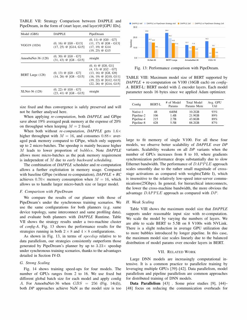
TABLE VII: Strategy Comparison between DAPPLE andPipeDream, in the form of (start layer, end layer)@[GPU IDs].

Model (GBS) DAPPLE PipeDream

VGG19 (1024) (0, 16) @ [G0 - G13](17, 25) @ [G14, G15]

(0, 11) @ [G0 - G7](11, 17) @ [G8 - G13](17, 19) @ G14(19, 25) @ G15

AmoebaNet-36 (128) (0, 30) @ [G0 - G7](31, 43) @ [G8 - G15] straight

BERT Large (128) (0, 13) @ [G0 - G7](14, 26) @ [G8 - G15]

(0, 4) @ [G0, G1](4, 13) @ [G2 - G7](13, 16) @ [G8, G9](16, 19) @ [G10, G11](19, 22) @ [G12, G13](22, 26) @ [G14, G15]

XLNet-36 (128) (0, 22) @ [G0 - G7](23, 41) @ [G8 - G15] straight

size fixed and thus convergence is safely preserved and willnot be further analysed here.

When applying re-computation, both DAPPLE and GPipesave about 19% averaged peak memory at the expense of 20%on throughput when keeping M = 2 fixed.

When both without re-computation, DAPPLE gets 1.6×higher throughput with M = 16, and consumes 0.88× aver-aged peak memory compared to GPipe, which only supportsup to 2 micro-batches. The speedup is mainly because higherM leads to lower proportion of bubbles. Note DAPPLEallows more micro-batches as the peak memory requirementis independent of M due to early backward scheduling.

The combination of DAPPLE scheduler and re-computationallows a further exploitation in memory usage. Comparedwith baseline GPipe (without re-computation), DAPPLE + RCachieves 0.70× memory consumption when M = 16, whichallows us to handle larger micro-batch size or larger model.

F. Comparison with PipeDream

We compare the results of our planner with those ofPipeDream’s under the synchronous training scenarios. Weuse the same configurations for both planners (e.g. samedevice topology, same interconnect and same profiling data),and evaluate both planners with DAPPLE Runtime. TableVII shows the strategy results under a two-machine clusterof config-A. Fig. 13 shows the performance results for thestrategies running in both 2× 8 and 4× 8 configurations.

As shown in Fig. 13, in terms of speedup relative to todata parallelism, our strategies consistently outperform thosegenerated by PipeDream’s planner by up to 3.23× speedupunder synchronous training scenarios, thanks to the advantagesdetailed in Section IV-D.

G. Strong Scaling

Fig. 14 shows training speed-ups for four models. Thenumber of GPUs ranges from 2 to 16. We use fixed butdifferent global batch size for each model and apply configA. For AmoebaNet-36 when GBS = 256 (Fig. 14(d)),both DP approaches achieve NaN as the model size is too

23.8 24.4

12.7

16.315.7

19.2

7.4

2.2

14.9 14.5

11.69.6

8.6

11.5

6.3

3.0

Spe

edup

0.0

10.0

20.0

30.0

XLNet-36 BERT-Large AmoebaNet-36 VGG-19

DAPPLE 4x8 DAPPLE w/ PipeDream Strategy 4x8 DAPPLE 2x8 DAPPLE w/ PipeDream Strategy 2x8

Fig. 13: Performance comparison with PipeDream.

TABLE VIII: Maximum model size of BERT supported byDAPPLE + re-computation on V100 (16GB each) on config-A. BERT-L: BERT model with L encoder layers. Each modelparameter needs 16 bytes since we applied Adam optimizer.

Config BERT-L # of ModelParams

Total ModelParams Mem

Avg. GPUUtil

Native-1 48 640M 10.2GB 93%Pipeline-2 106 1.4B 21.9GB 89%Pipeline-4 215 2.7B 43.8GB 89%Pipeline-8 428 5.5B 88.2GB 87%

large to fit memory of single V100. For all these fourmodels, we observe better scalability of DAPPLE over DPvariants. Scalability weakens on all DP variants when thenumber of GPUs increases from 8 to 10, where gradientssynchronization performance drops substantially due to slowEthernet bandwidth. The performance of DAPPLE approachscales smoothly due to the rather small magnitude of cross-stage activations as compared with weights(Table I), whichis insensitive to the relatively low-speed inter-server commu-nications(25Gbps). In general, for hierarchical interconnects,the lower the cross-machine bandwidth, the more obvious theadvantage DAPPLE approach as compared with DP .

H. Weak Scaling

Table VIII shows the maximum model size that DAPPLEsupports under reasonable input size with re-computation.We scale the model by varying the numbers of layers. Weare able to scale BERT to 5.5B on 8 V100s with NVLink.There is a slight reduction in average GPU utilization dueto more bubbles introduced by longer pipeline. In this case,the maximum model size scales linearly due to the balanceddistribution of model params over encoder layers in BERT.

VII. RELATED WORK

Large DNN models are increasingly computational in-tensive. It is a common practice to parallelize training byleveraging multiple GPUs [39]–[42]. Data parallelism, modelparallelism and pipeline parallelism are common approachesfor distributed training of DNN models.

Data Parallelism [43] . Some prior studies [9], [44]–[48] focus on reducing the communication overheads for

0

4

8

12

16

2 4 6 8 10 12 14 16

Trai

ning

Spee

dup

Number of GPUs

DP No OverlapDP+Normal OverlapBest Hybrid SpeedupStraight Pipeline

(a) GNMT-16(GBS = 2048)

0

4

8

12

16

2 4 6 8 10 12 14 16

Trai

ning

Spee

dup

Number of GPUs

DP No OverlapDP+Normal OverlapBest Hybrid Speedup

(b) BERT-48(GBS = 128)

0

4

8

12

16

2 4 6 8 10 12 14 16

Trai

ning

Spee

dup

Number of GPUs

DP No OverlapDP+Normal OverlapBest Hybrid Speedup

(c) XLNet-36(GBS = 128)

0

4

8

12

16

2 4 6 8 10 12 14 16

Trai

ning

Spee

dup

Number of GPUs

DP No OverlapDP+Normal OverlapBest Hybrid Speedup

(d) AmoebaNet-36(GBS = 256)

Fig. 14: Speedup with fixed GBS in config-A.

data parallelism. As a commonly used performance optimiza-tion method, gradients accumulation [5], [6], [49] offers aneffective approach to reduce communication-to-computationratio. Another complementary approach is computation andcommunication overlap, with promising results reported insome CNN benchmarks [8], [20].

Model Parallelism. Model Parallelism [50] partitions DNNmodels among GPUs to mitigate communication overhead andmemory bottlenecks for distributed training [10], [14], [39],[40], [51]–[54]. This paper focuses on model partition betweenlayers, namely, pipeline parallelism.

Pipeline parallelism. Pipeline Parallelism [10], [11], [14],[21], [55] has been recently proposed to train DNN in apipelined manner. GPipe [10] explores synchronous pipelineapproach to train large models with limited GPU memory.PipeDream [14] explores the hybrid approach of data andpipeline parallelism for asynchronous training. [53], [55], [56]make further optimization based on PipeDream. Pal et al.[40] evaluated the hybrid approach without thorough study.Some researchers have been seeking for the optimal placementstrategy to assign operations in a DNN to different devices[57]–[59] to further improve system efficiency.

VIII. CONCLUSION

In this paper, we propose DAPPLE framework for pipelinedtraining of large DNN models. DAPPLE addresses the need forsynchronous pipelined training and advances current state-of-the-art by novel pipeline planning and micro-batch schedulingapproaches. On one hand, DAPPLE planner module deter-mines an optimal parallelization strategy given model structureand hardware configurations. It considers pipeline partition,replication and placement, and generates a high-performancehybrid data/pipeline parallel strategy. On the other hand,DAPPLE scheduler module is capable of simultaneouslyachieving optimal training efficiency and moderate memoryconsumption, without storing multiple versions of parametersand getting rid of the strong demand of re-computation whichhurts system efficiency at the same time. Experiments showthat DAPPLE planner consistently outperforms strategies gen-erated by PipeDreams planner by up to 3.23× speedup undersynchronous training scenarios, and DAPPLE scheduler out-performs GPipe by 1.6× speedup of training throughput andsaves 12% of memory consumption at the same time.

REFERENCES

[1] R. Sutton, The Bitter Lesson, 2019, http://www.incompleteideas.net/IncIdeas/BitterLesson.html.

[2] C. Raffel, N. Shazeer, A. Roberts, K. Lee, S. Narang, M. Matena,Y. Zhou, W. Li, and J. P. Liu, “Exploring the limits of transfer learningwith a unified text-to-text transformer,” https://arxiv.org/abs/1910.10683,2019.

[3] J. Wang, P. Huang, H. Zhao, Z. Zhang, B. Zhao, and D. L. Lee,“Billion-scale commodity embedding for e-commerce recommendationin alibaba,” in Proceedings of the 24th ACM SIGKDD InternationalConference on Knowledge Discovery and Data Mining. ACM, 2018,pp. 839–848.

[4] P. Covington, J. Adams, and E. Sargin, “Deep neural networks foryoutube recommendations,” in Proceedings of the 10th ACM Conferenceon Recommender Systems, ACM, New York, NY, USA. ACM, 2016.

[5] Gradients Accumulation-Tensorflow, 2019, https://github.com/tensorflow/tensorflow/pull/32576.

[6] Gradients Accumulation-PyTorch, 2019, https://gist.github.com/thomwolf/ac7a7da6b1888c2eeac8ac8b9b05d3d3.

[7] A New Lightweight, Modular, and Scalable Deep Learning Framework,2016, https://caffe2.ai/.

[8] A. Jayarajan, J. Wei, G. Gibson, A. Fedorova, and G. Pekhimenko,“Priority-based parameter propagation for distributed dnn training,”arXiv preprint arXiv:1905.03960, 2019.

[9] A. Sergeev and M. Del Balso, “Horovod: fast and easy distributed deeplearning in tensorflow,” arXiv preprint arXiv:1802.05799, 2018.

[10] Y. Huang, Y. Cheng, A. Bapna, O. Firat, D. Chen, M. Chen, H. Lee,J. Ngiam, Q. V. Le, Y. Wu et al., “Gpipe: Efficient training of giantneural networks using pipeline parallelism,” in Advances in NeuralInformation Processing Systems, 2019, pp. 103–112.

[11] J. Zhan and J. Zhang, “Pipe-torch: Pipeline-based distributed deeplearning in a gpu cluster with heterogeneous networking,” in 2019Seventh International Conference on Advanced Cloud and Big Data(CBD). IEEE, 2019, pp. 55–60.

[12] D. Narayanan, A. Harlap, A. Phanishayee, V. Seshadri, N. R. Devanur,G. R. Ganger, P. B. Gibbons, and M. Zaharia, “Pipedream: generalizedpipeline parallelism for dnn training,” in Proceedings of the 27th ACMSymposium on Operating Systems Principles. ACM, 2019, pp. 1–15.

[13] T. Chen, B. Xu, C. Zhang, and C. Guestrin, “Training deep nets withsublinear memory cost,” arXiv preprint arXiv:1604.06174, 2016.

[14] A. Harlap, D. Narayanan, A. Phanishayee, V. Seshadri, N. Devanur,G. Ganger, and P. Gibbons, “Pipedream: Fast and efficient pipelineparallel dnn training,” arXiv preprint arXiv:1806.03377, 2018.

[15] M. Wang, C. Meng, G. Long, C. Wu, J. Yang, W. Lin, and Y. Jia,“Characterizing deep learning training workloads on alibaba-pai,” arXivpreprint arXiv:1910.05930, 2019.

[16] GpipeTalk, 2019, https://www.youtube.com/watch?v=9s2cum25Kkc.[17] P. Goyal, P. Dollar, R. Girshick, P. Noordhuis, L. Wesolowski, A. Kyrola,

A. Tulloch, Y. Jia, and K. He, “Accurate, large minibatch sgd: Trainingimagenet in 1 hour,” arXiv preprint arXiv:1706.02677, 2017.

[18] G. Long, J. Yang, K. Zhu, and W. Lin, “Fusionstitching: Deepfusion and code generation for tensorflow computations on gpus,”https://arxiv.org/abs/1811.05213, 2018.

[19] G. Long, J. Yang, and W. Lin, “Fusionstitching: Boosting execu-tion efficiency of memory intensive computations for dl workloads,”https://arxiv.org/abs/1911.11576, 2019.

[20] H. Zhang, Z. Zheng, S. Xu, W. Dai, Q. Ho, X. Liang, Z. Hu,J. Wei, P. Xi, and E. P. Xing, “Poseidon: An efficient communicationarchitecture for distributed deep learning on GPU clusters,” in 2017USENIX Annual Technical Conference (USENIX ATC 17). SantaClara, CA: USENIX Association, Jul. 2017, pp. 181–193. [Online].Available: https://www.usenix.org/conference/atc17/technical-sessions/presentation/zhang

[21] B. Yang, J. Zhang, J. Li, C. Re, C. R. Aberger, and C. De Sa,“Pipemare: Asynchronous pipeline parallel dnn training,” arXiv preprintarXiv:1910.05124, 2019.

[22] NVLink, 2019, https://www.nvidia.com/en-us/data-center/nvlink/.[23] H. Lee, M. Jeong, C. Kim, S. Lim, I. Kim, W. Baek, and B. Yoon,

“torchgpipe, A GPipe implementation in PyTorch,” https://github.com/kakaobrain/torchgpipe, 2019.

[24] I. Barany and V. S. Grinberg, “Block partitions of sequences,” IsraelJournal of Mathematics, vol. 206, no. 1, pp. 155–164, 2015.

[25] M. Abadi, A. Agarwal, P. Barham, E. Brevdo, Z. Chen, C. Citro, G. S.Corrado, A. Davis, J. Dean, M. Devin, S. Ghemawat, I. Goodfellow,A. Harp, G. Irving, M. Isard, Y. Jia, R. Jozefowicz, L. Kaiser,M. Kudlur, J. Levenberg, D. Mane, R. Monga, S. Moore, D. Murray,C. Olah, M. Schuster, J. Shlens, B. Steiner, I. Sutskever, K. Talwar,P. Tucker, V. Vanhoucke, V. Vasudevan, F. Viegas, O. Vinyals,P. Warden, M. Wattenberg, M. Wicke, Y. Yu, and X. Zheng,“TensorFlow: Large-scale machine learning on heterogeneous systems,”2015, software available from tensorflow.org. [Online]. Available:http://tensorflow.org/

[26] J. Demouth, “Cuda pro tip: Minimize the tail ef-fect,” 2015. [Online]. Available: https://devblogs.nvidia.com/cuda-pro-tip-minimize-the-tail-effect/

[27] R. Sennrich, B. Haddow, and A. Birch, “Edinburgh neural machinetranslation systems for wmt 16,” arXiv preprint arXiv:1606.02891, 2016.

[28] P. Rajpurkar, R. Jia, and P. Liang, “Know what you don’t know:Unanswerable questions for squad,” arXiv preprint arXiv:1806.03822,2018.

[29] O. Russakovsky, J. Deng, H. Su, J. Krause, S. Satheesh, S. Ma,Z. Huang, A. Karpathy, A. Khosla, M. Bernstein et al., “Imagenet largescale visual recognition challenge,” International journal of computervision, vol. 115, no. 3, pp. 211–252, 2015.

[30] Y. Wu, M. Schuster, Z. Chen, Q. V. Le, M. Norouzi, W. Macherey,M. Krikun, Y. Cao, Q. Gao, K. Macherey et al., “Google’s neuralmachine translation system: Bridging the gap between human andmachine translation,” arXiv preprint arXiv:1609.08144, 2016.

[31] J. Devlin, M.-W. Chang, K. Lee, and K. Toutanova, “Bert: Pre-trainingof deep bidirectional transformers for language understanding,” arXivpreprint arXiv:1810.04805, 2018.

[32] Z. Yang, Z. Dai, Y. Yang, J. Carbonell, R. Salakhutdinov, and Q. V. Le,“Xlnet: Generalized autoregressive pretraining for language understand-ing,” arXiv preprint arXiv:1906.08237, 2019.

[33] K. He, X. Zhang, S. Ren, and J. Sun, “Deep residual learning for imagerecognition,” in Proceedings of the IEEE conference on computer visionand pattern recognition, 2016, pp. 770–778.

[34] K. Simonyan and A. Zisserman, “Very deep convolutional networks forlarge-scale image recognition,” arXiv preprint arXiv:1409.1556, 2014.

[35] S. A. R. Shah, W. Wu, Q. Lu, L. Zhang, S. Sasidharan, P. DeMar,C. Guok, J. Macauley, E. Pouyoul, J. Kim et al., “Amoebanet: An sdn-enabled network service for big data science,” Journal of Network andComputer Applications, vol. 119, pp. 70–82, 2018.

[36] NCCL, 2019, https://developer.nvidia.com/nccl.[37] D. P. Kingma and J. Ba, “Adam: A method for stochastic optimization,”

arXiv preprint arXiv:1412.6980, 2014.[38] T. Tieleman and G. Hinton, “Lecture 6.5-rmsprop: Divide the gradient

by a running average of its recent magnitude,” COURSERA: NeuralNetworks for Machine Learning 4, 2012.

[39] J. Dean, G. Corrado, R. Monga, K. Chen, M. Devin, M. Mao, M. Ran-zato, A. Senior, P. Tucker, K. Yang et al., “Large scale distributed deepnetworks,” in Advances in neural information processing systems, 2012,pp. 1223–1231.

[40] S. Pal, E. Ebrahimi, A. Zulfiqar, Y. Fu, V. Zhang, S. Migacz, D. Nellans,and P. Gupta, “Optimizing multi-gpu parallelization strategies for deeplearning training,” IEEE Micro, vol. 39, no. 5, pp. 91–101, 2019.

[41] Z. Jia, S. Lin, C. R. Qi, and A. Aiken, “Exploring the hidden dimensionin accelerating convolutional neural networks,” 2018.

[42] J. Geng, D. Li, and S. Wang, “Horizontal or vertical?: A hybrid approachto large-scale distributed machine learning,” in Proceedings of the 10thWorkshop on Scientific Cloud Computing. ACM, 2019, pp. 1–4.

[43] A. Krizhevsky, “One weird trick for parallelizing convolutional neuralnetworks,” arXiv preprint arXiv:1404.5997, 2014.

[44] Baidu-allreduce, 2018, https://github.com/baidu-research/baidu-allreduce.

[45] X. Jia, S. Song, W. He, Y. Wang, H. Rong, F. Zhou, L. Xie, Z. Guo,Y. Yang, L. Yu et al., “Highly scalable deep learning training systemwith mixed-precision: Training imagenet in four minutes,” arXiv preprintarXiv:1807.11205, 2018.

[46] N. Arivazhagan, A. Bapna, O. Firat, D. Lepikhin, M. Johnson,M. Krikun, M. X. Chen, Y. Cao, G. Foster, C. Cherry et al., “Mas-sively multilingual neural machine translation in the wild: Findings andchallenges,” arXiv preprint arXiv:1907.05019, 2019.

[47] Byteps, A high performance and generic framework for distributed DNNtraining, 2019, https://github.com/bytedance/byteps.

[48] Y. You, J. Hseu, C. Ying, J. Demmel, K. Keutzer, and C.-J. Hsieh,“Large-batch training for lstm and beyond,” in Proceedings of theInternational Conference for High Performance Computing, Networking,Storage and Analysis, 2019, pp. 1–16.

[49] T. D. Le, T. Sekiyama, Y. Negishi, H. Imai, and K. Kawachiya,“Involving cpus into multi-gpu deep learning,” in Proceedings of the2018 ACM/SPEC International Conference on Performance Engineer-ing. ACM, 2018, pp. 56–67.

[50] Z. Jia, M. Zaharia, and A. Aiken, “Beyond data and model parallelismfor deep neural networks,” arXiv preprint arXiv:1807.05358, 2018.

[51] Z. Huo, B. Gu, Q. Yang, and H. Huang, “Decoupled parallel backprop-agation with convergence guarantee,” arXiv preprint arXiv:1804.10574,2018.

[52] J. Geng, D. Li, and S. Wang, “Rima: An rdma-accelerated model-parallelized solution to large-scale matrix factorization,” in 2019 IEEE35th International Conference on Data Engineering (ICDE). IEEE,2019, pp. 100–111.

[53] C.-C. Chen, C.-L. Yang, and H.-Y. Cheng, “Efficient and robust paralleldnn training through model parallelism on multi-gpu platform,” arXivpreprint arXiv:1809.02839, 2018.

[54] N. Dryden, N. Maruyama, T. Moon, T. Benson, M. Snir, and B. Van Es-sen, “Channel and filter parallelism for large-scale cnn training,” inProceedings of the International Conference for High PerformanceComputing, Networking, Storage and Analysis, 2019, pp. 1–20.

[55] J. Geng, D. Li, and S. Wang, “Elasticpipe: An efficient and dynamicmodel-parallel solution to dnn training,” in Proceedings of the 10thWorkshop on Scientific Cloud Computing. ACM, 2019, pp. 5–9.

[56] L. Guan, W. Yin, D. Li, and X. Lu, “Xpipe: Efficient pipeline model par-allelism for multi-gpu dnn training,” arXiv preprint arXiv:1911.04610,2019.

[57] A. Mirhoseini, H. Pham, Q. V. Le, B. Steiner, R. Larsen, Y. Zhou,N. Kumar, M. Norouzi, S. Bengio, and J. Dean, “Device placementoptimization with reinforcement learning,” in Proceedings of the 34thInternational Conference on Machine Learning-Volume 70. JMLR. org,2017, pp. 2430–2439.

[58] J. Gu, M. Chowdhury, K. G. Shin, Y. Zhu, M. Jeon, J. Qian, H. Liu,and C. Guo, “Tiresias: A {GPU} cluster manager for distributed deeplearning,” in 16th {USENIX} Symposium on Networked Systems Designand Implementation ({NSDI} 19), 2019, pp. 485–500.

[59] M. Wang, C.-c. Huang, and J. Li, “Supporting very large models usingautomatic dataflow graph partitioning,” in Proceedings of the FourteenthEuroSys Conference 2019, 2019, pp. 1–17.