daniele samuel pascovici “thermo economic and risk
TRANSCRIPT

I
Daniele Samuel Pascovici
“Thermo Economic and Risk Analysis for Advanced Long
Range Aero Engines”
School of Engineering
PhD Thesis
CORE Metadata, citation and similar papers at core.ac.uk
Provided by Cranfield CERES

II
Daniele Samuel Pascovici
“Thermo Economic and Risk Analysis for Advanced Long
Range Aero Engines”
Supervisors:
Prof. Riti Singh
Dr. Stephen Ogaji
December 2008
This thesis is submitted in partial fulfilment of the requirements for the
Degree of Doctor of Philosophy

III
To improve yourself and your knowledge
Frank Nopple

IV
Executive Summary
To conceive and assess engines with minimum global warming impact and
lowest cost of ownership in a variety of emission legislation scenarios,
emissions taxation policies, fiscal and Air Traffic Management environments a
Techno economic and Environmental Risk Assessment (TERA) model is
needed.
In the first part of this thesis an approach is presented to estimate the cost of
maintenance and the direct operating costs of turbofan engines of equivalent
thrust rating, both for long and short range applications. The three advanced
types of turbofan engines analysed here are a direct drive three spool with
ultra high bypass ratio, a geared turbofan with the same fan as the direct drive
engine and a turbofan with counter rotating fans. The baseline engines are a
three spool for long range (Trent 772b) and a two spool (CFM56-7b) for short
range applications. The comparison with baseline engines shows the gains
and losses of these novel cycle engines.
The economic model is composed of three modules: a lifing module, an
economic module and a risk module.
The lifing module estimates the life of the high pressure turbine disk and
blades through the analysis of creep and fatigue over a full working cycle of
the engine. These two phenomena are usually the most limiting factors to the
life of the engine. The output of this module is the amount of hours that the
engine can sustain before its first overhaul (called time between overhauls).
The value of life calculated by the lifing is then taken as the baseline
distribution to calculate the life of other important modules of the engine using
the Weibull approach. The Weibull formulation is applied to the life analysis of
different parts of the engine in order to estimate the cost of maintenance, the
direct operating costs (DOC) and net present cost (NPC) of turbofan engines.
The Weibull distribution is often used in the field of life data analysis due to its
flexibility—it can mimic the behavior of other statistical distributions such as

V
the normal and the exponential. In the present work five Weibull distributions
are used for five important sources of interruption of the working life of the
engine: Combustor, Life Limited Parts (LLP), High Pressure Compressor
(HPC), General breakdowns and High Pressure Turbine (HPT). The Weibull
analysis done in this work shows the impact of the breakdown of different
parts of the engine on the NPC and DOC, the importance that each module of
the engine has in its life, and how the application of the Weibull theory can
help us in the risk assessment of future aero engines.
Then the lower of the values of life of all the distributions is taken as time
between overhaul (TBO), and used into the economic module calculations.
The economic module uses the time between overhaul together with the cost
of labour and the cost of the engine (needed to determine the cost of spare
parts) to estimate the cost of maintenance of the engine. The direct operating
costs (DOC) of the engine are derived as a function of maintenance cost with
the cost of taxes on emissions and noise, the cost of fuel, the cost of
insurance and the cost of interests paid on the total investment. The DOC of
the aircraft include also the cost of cabin and flight crew and the cost of
landing, navigational and ground handling fees. With knowledge of the DOC
the net present cost (NPC) for both the engine and the aircraft can be
estimated over an operational period of about 30 years.
The risk model uses the Monte Carlo method with a Gaussian distribution to
study the impact of the variations in some parameters on the NPC. Some of
the parameters considered in the risk scenarios are fuel price, interest
percentage on total investment, inflation, downtime, maintenance labour cost
and factors used in the emission and noise taxes. The risk analyses the
influence of these variables for ten thousands scenarios and then a
cumulative frequency curve is built by the model to understand the frequency
of the most probable scenarios.
After the conclusion of the analysis of the VITAL engines as they were
specified by the Original Engine Manufacturer (OEM) (Roll – Royce, Snecma
and MTU), an optimisation work was done in order to try to improve the

VI
engines. The optimisation was done using two numerical gradient based
techniques Firstly the Sequential Quadratic Programming – NLPQL and
secondly the Mixed Integer Optimization – MOST; the objectives of the
optimisation were two: minimum fuel burn and minimum direct operating
costs. Because the engines were already optimized for minimum fuel burn,
the optimization for minimum fuel burn didn’t show any meaningful results;
instead the results for minimum DOC showed that the engines can have some
improvements.
The ability of the three VITAL configurations to meet the future goals of the
European Union to reduce noise and gaseous emission has been assessed
and has showed that the three engines cannot fully comply with future
legislation beyond 2020.
In the second part of this thesis three further advanced configurations have
been studied to determine whether these are potential solutions to meet the
ACARE goals of 2020.
For these more advanced aero engines only a performance and gaseous
emissions analysis has been done, because it was no possible to do an
economic analysis for the new components of these engines. These
advanced configurations feature components that have been studied only in
laboratories, like the heat exchangers for the ICR, the wave rotor and the
constant volume combustor, and for these it has not been done a lifing
analysis that is fundamental in order to understand the costs of maintenance,
besides in order to do a proper direct operating costs analysis many
operational flight hours are needed and none of these engine have reached
TRL of 7 and more which is the stage where flight hour tests are conducted.
In this thesis a parametric study on three different novel cycles which could be
applied to aircraft propulsion is presented:
1. Intercooled recuperative,
2. wave rotor and

VII
3. Constant volume combustion cycle.
These three cycles have been applied to a characteristic next generation long
range aero engine (geared turbofan) looking for a possible future evolution
and searching for benefits on specific thrust fuel consumption and emissions.
The parametric study has been applied to Top of Climb conditions, the design
point, at Mach number 0.82, ISA deviation of 10 degrees and an altitude of
10686 m and at cruise condition, considering two possible designs:
a) Design for constant specific thrust and
b) Design for constant TET or the current technology level
Both values correspond to the baseline engine. For the intercooled engine
also a weight and drag impact on fuel consumption has been done, in order to
understand the impact of weight increase on the benefits of the configuration,
considering different values of the effectiveness of the heat exchangers, the
higher the values the greater is the technical challenge of the engine.
After studying the CVC and Wave rotor separately it has been decided to do a
parametric study of an aero engine that comprises both configurations: the
internal combustion wave rotor (ICWR). The ICWR is a highly unsteady
device, but offers significant advantages when combined with gas turbines.
Since it is a constant volume combustion device there is a pressure raise
during combustion, this will result in having lower SFC and higher thermal
efficiency. It is an advanced and quite futuristic, with a technology readiness
level (TRL) of 6 or higher only by 2025, so only a preliminary performance
study is done, leaving to future studies the task of a more improved analysis.

VIII
Acknowledgements
My greatest gratitude goes to professors Pericles Pilidis and Riti Singh which
gave me the opportunity to do this PhD, and Dr Stephen Ogaji, which helped
me in every way possible throughout all the doctorate period, always showing
great patience and a deep insight of my problems, guiding me perfectly in
their solutions.
I want to thank Prof. Gregorio Corchero that gave me the possibility to work
with him in Madrid; it was a fantastic period by every mean.
Then I want to thank Oliviero Vigna Suria, not only he helped me a lot in the
realization of the lifing module, but also for being a true friend.
A list of all the friends with whom I have shared this journey would be too
long, but they know who they are and I have thanked them many times.
I want to thank also my Mother that was always with me in these times, good
and bad.
And last, but not least, I want to thank my good friend Frank Nopple, without
his words and counsel I wouldn’t have ever started this PhD, which has been
so far the greatest adventure of my life.

IX
Table of Contents
1. INTRODUCTION.........................................................................................................................1
1.1 ENVIRONMENTALLY FRIENDLY AERO ENGINES (VITAL) ....................................................1
1.1.1 Progress against the state-of-the-art .....................................................................................4
1.1.2 The trend of increasing BPR..................................................................................................5
1.1.3 Decreasing the fan tip speed..................................................................................................6
1.2 THESIS STRUCTURE ..............................................................................................................8
2. LITERATURE SURVEY............................................................................................................10
2.1 THE ECONOMIC MODULE....................................................................................................11
2.1.1 The Roskam Method .......................................................................................................11
2.1.2 The Jenkinson Method .........................................................................................................14
2.1.4 Engine lifing.........................................................................................................................16
2.1.4.1 Sources and analysis of stresses on blades and disk.........................................................16
2.1.4.2 Cooling model...................................................................................................................18
2.1.4.3 Thermal Barrier coating ...................................................................................................22
2.1.4.4 FAILURE MECHANISMS ................................................................................................23
2.1.4.5 LOW CYCLE FATIGUE ...................................................................................................25
2.1.4.5.1 General theory ........................................................................................ 252.1.4.5.2 Low cycle fatigue analysis: Coffin-Manson method................................ 282.1.4.5.3 Fatigue material properties: a statistical approach ................................. 31
2.1.4.6 CREEP..............................................................................................................................33
2.1.4.6.1 General theory ........................................................................................ 342.1.4.6.2 Approaching time-temperature method to creep analysis ...................... 352.1.4.6.3 Cumulative Creep ................................................................................... 362.1.4.6.4 Limitations and considerations................................................................ 37
2.1.5 Weibull Distribution.............................................................................................................38
2.1.5.1 Generating Weibull distributed random variates..............................................................40
2.2 MONTE CARLO SIMULATION TECHNIQUE...........................................................................42
2.3 INTRODUCTION TO OPTIMISATION ......................................................................................42
2.3.1 Numerical Optimisation Techniques....................................................................................43
2.3.1.1 Direct Methods ........................................................................................... 432.3.1.2 Penalty Methods ........................................................................................ 45
2.3.2 Exploratory Techniques .......................................................................................................46
2.4 ADVANCED AERO ENGINES ................................................................................................47
2.5 MORE FUTURE ENGINE: THE INTERNAL COMBUSTION WAVE ROTOR .................................50
2.5.1 Advantages and Limitations of the Internal Combustion Wave Rotor .................................54
3. ECONOMIC MODULE ..............................................................................................................57
3.1 METHODOLOGY ...................................................................................................................58
3.2 ECONOMIC MODULE DESCRIPTION ....................................................................................64

X
3.2.1 Economic Module Architecture ......................................................................................64
3.2.2 Module Requirement Definition...........................................................................................64
3.2.3 Input file Definition..............................................................................................................65
3.2.4 Output Files .........................................................................................................................67
3.3 THE LIFING MODULE ...........................................................................................................68
3.3.1 Structure of the lifing module...............................................................................................69
3.3.1 STRESS ANALYSIS ..............................................................................................................71
3.3.1.1 Blade stress analysis module ........................................................713.3.1.2 Disc stress analysis module ...........................................................72
3.3.2 Application of cooling within the code.................................................................................74
3.3.3 Low cycle fatigue module.....................................................................................................75
3.3.4 Creep module .......................................................................................................................78
4. ADVANCED PROPULSION SYSTEMS ................................................................................81
4.1 CANDIDATE CYCLES DESCRIPTION ....................................................................................81
4.2 PERFORMANCE MODEL .......................................................................................................86
5. RESULTS AND DISCUSSIONS..............................................................................................92
5.1 THE ECONOMIC MODULE....................................................................................................92
5.2 RESULTS OF THE WEIBULL MODULE ...............................................................................100
5.2.1 Engine Components description. .......................................................................................100
5.2.2 Engines Description and outcome of the analysis..............................................................101
5.3 OPERATING COST AND RISK ANALYSIS FOR AERO ENGINES.........................................105
5.3.1 Baseline and Future Engines description ..........................................................................105
5.3.2 Results ................................................................................................................................108
5.4 VITAL ENGINES OPTIMIZATION RESULTS .......................................................................112
5.5 RESULTS OF THE ADVANCED PROPULSION SYSTEMS ......................................................113
5.5.1 Results for designs at Top of Climb ...................................................................................115
5.5.1.1 The IRC cycle........................................................................................... 1155.5.1.2 The WRTC cycle ...................................................................................... 1205.5.1.3 The CV cycle............................................................................................ 123
5.5.2 Results for cruise................................................................................................................128
5.5.3 Discussion..........................................................................................................................131
5.6 THE INTERNAL COMBUSTION WAVE ROTOR (ICWR)........................................................136
5.6.1 Assumptions .......................................................................................................................136
5.6.2 Result .................................................................................................................................137
6. CONCLUSIONS AND RECOMMENDATIONS...................................................................141
6.1 CONCLUSIONS...................................................................................................................141
6.2 RECOMMENDATIONS FOR FUTURE WORKS.......................................................................145
6.3 AUTHOR’S CONTRIBUTIONS TO KNOWLEDGE ...................................................................146
REFERENCES...................................................................................................................................148

XI
APPENDIX A – ECONOMIC MODEL INPUT FILES...................................................................154
APPENDIX B – ECONOMIC MODEL OUTPUT FILES ..............................................................159
APPENDIX C: TURBOMATCH INPUT FILES .............................................................................161
APPENDIX D: ISIGHT ......................................................................................................................165
APPENDIX E - PUBLICATIONS ....................................................................................................168
APPENDIX F – EQUATIONS USED IN THE ECONOMIC MODULE.......................................170
F.1 Economic Module.................................................................................................................170
F.2 Gaussian Distribution Module .............................................................................................171
F.3 Weibull Distribution Module ................................................................................................171
F.4 Fatigue Module ....................................................................................................................172
F.5 Creep Module .......................................................................................................................174
F.6 Disk Stress Module ...............................................................................................................180
F.7 Blade Stess Module...............................................................................................................184

XII
List of Figures
Figure 1: Noise vs. BPR (VITAL 2004) ....................................................................4
Figure 2: BPR and fuel burn penalties (VITAL 2004) ............................................5
Figure 3: Weight and BPR (VITAL 2004) ................................................................6
Figure 4: trends in aircraft noise reduction (VITAL 2004).....................................7
Figure 5: fan concepts in VITAL and SILENCE® (VITAL 2004)..........................7
Figure 6 Direct operating cost (DOC) components (Jenkinson 1999)..............14
Figure 7 Varying thickness disc (Haslam 2006)...................................................18
Figure 8 Typical turbine cooling system (Haslam 2006).....................................19
Figure 9 Thermal barrier coating principles ..........................................................22
Figure 10, S-N curve for brittle aluminium.............................................................26
Figure 11 Typical Strain-Life curves.......................................................................29
Figure 12 Coffin-Manson curves of 81 aluminium and 15 titanium alloys
(Meggiolaro and Castro 2004). ...............................................................................33
Figure 13 the General Creep Curve......................................................................35
Figure 14 Density function for the five components of the engine ....................40
Figure 15 NPC and Cumulative distributions for the four engines ....................41
Figure 16: CVC machinery exploded view (Smith et al 2002) ...........................52
Figure 17 general arrangement of the CVC (Smith et al 2002) .........................52
Figure 18 developed view of the CVC process (Smith et al 2002) ...................53
Figure 19 conventional versus CVC engine (Smith et al 2002).........................54
Figure 20 Direct operating cost (DOC) components (Jenkinson 1999) ...........59
Figure 21 Cumulative curve for the net present cost (NPC) ..............................62
Figure 22: the TERA structure (TERA 2006) ........................................................63
Figure 23 Economic Module Structure ..................................................................64

XIII
Figure 24, Lifing Module Breakdown (Vigna Suria 2006) ...................................69
Figure 25 Creep and Low cycle fatigue life for different types of mission........70
Figure 26 Blade stress module structure (Vigna Suria 2006) ............................71
Figure 27 Disc stress module structure (Vigna Suria 2006)...............................72
Figure 28 Blade cooling sub-module structure. (Vigna Suria 2006) .................74
Figure 29 Low Cycle Fatigue module structure (Vigna Suria 2006) .................76
Figure 30 Creep module structure (Vigna Suria 2006) .......................................79
Figure 31 the Intercooled Recuperated Cycle .......................................................82
Figure 32 the Wave Rotor Cycle.............................................................................84
Figure 33 the Constant Volume Combustion Cycle.............................................85
Figure 34 Cumulative curve for the net present cost (NPC) ..............................94
Figure 35 Costs of maintenance division between labour cost and materials
cost ..............................................................................................................................94
Figure 36 Cost of maintenance for short range engines currently in use ........95
Figure 37 Cost of maintenance for long range engines currently in use..........96
Figure 38 Change of the fuel price with inflation over a period of 30 years.....96
Figure 39: impact on DOC with the change of values of the economic inputs97
Figure 40 influence of economic parameters according to the risk analysis for
long range engines ...................................................................................................99
Figure 41 growing of the maintenance cost in the next 30 years.................................99
Figure 42 NPC and Frequency for the four engines..........................................105
Figure 43 Causes of engine breakdown (Pareto Diagram) ..............................105
Figure 44 Schematic of the DDTF .........................................................................106
Figure 45: Preliminary counter-rotating turbofan (CRTF). (Baudier 2004) ....107
Figure 46 Comparison of costs for the long range engines .............................111
Figure 47 Comparison of costs for short range engines...................................112
Figure 48 Optimisation results for the GTFLR for the economic parameters113

XIV
Figure 49 Optimisation results for the DDTFLR for the economic parameters
....................................................................................................................................113
Figure 50 – Influence of the overall pressure ratio and the regenerative
thermal efficiency (0.9, .., 0.7) on the SFC at ToC and for constant ST design
and cooling bled before RHE ................................................................................117
Figure 51 – Influence of the overall pressure ratio and the regenerative
thermal efficiency (0.9, ..,0.7) on the SFC at ToC and for constant ST design
and cooling bled at the exit of the RHE ...............................................................117
Figure 52 – Influence of the overall pressure ratio and the regenerative
thermal efficiency (0.9, ..,0.7) on the cooling availability at ToC for constant
ST design and cooling bled before RHE .............................................................118
Figure 53 – Influence of the overall pressure ratio and the regenerative
thermal efficiency (0.9, ..,0.7) on the cooling availability at TOC for constant
ST design and cooling bled at the exit of the RHE ............................................118
Figure 54 – Influence of the overall pressure ratio and the regenerative
thermal efficiency (0.9, ..,0.7) on the TET decrease at TOC for constant ST
design and cooling bled before of the RHE ........................................................119
Figure 55 – Relative variation of the NOx with the overall pressure ratio and
the regenerative thermal efficiency (0.9, .., 0.7) on the SFC at TOC and for
constant ST design and cooling bled before RHE .............................................119
Figure 56 – Influence of the overall pressure ratio and the regenerative
thermal efficiency (0.9, ..,0.7) on the SFC at TOC and for constant TET design
and cooling bled at the exit of the RHE ...............................................................120
Figure 57 – Gain of ST with the overall pressure ratio and the regenerative
thermal efficiency (0.9, ..,0.7) at TOC and for constant TET design and
cooling bled at the exit of the RHE .......................................................................120
Figure 58 – Variation of the overall pressure ration with wave rotor pressure
ratio for constant TET design (TET) and for constant ST design (ST) at TOC
....................................................................................................................................122

XV
Figure 59 – Increase of the maximum cycle temperature with wave rotor
pressure ratio for constant TET design (TET) and for constant ST design (ST)
at TOC.......................................................................................................................122
Figure 60 – Influence of the wave rotor pressure ratio on the SFC for constant
ST design (ST) and for constant ST design (ST) at TOC.................................122
Figure 61 – Gain of turbine entry temperature (TET) with wave rotor pressure
ratio for constant TET design (TET) and for constant ST design (ST) at TOC
....................................................................................................................................123
Figure 62 – Influence of the wave rotor pressure ration on the NOx for
constant TET design (TET) and for constant ST design (ST) at TOC............123
Figure 63 – Influence of the overall pressure ratio and the combustor pressure
losses on SFC for CV cycle and constant ST design at TOC..........................126
Figure 64 – Influence of the overall pressure ratio and the heat transferred to
the bypass in combustor cooling process on SFC for CV cycle and constant
ST design at TOC....................................................................................................126
Figure 65 – Variation of the overall pressure ratio with the HPC pressure ratio
for the CV cycle and constant ST design at TOC ..............................................127
Figure 66 – Influence of the overall pressure ratio and the heat transferred to
bypass in the combustor cooling process on NOx emission for the CV cycle
and constant ST design at TOC ...........................................................................127
Figure 67 – Gain on turbine entry temperature with the overall pressure ratio
and the heat transferred to bypass in the combustor cooling process for CV
cycle and constant ST design at TOC .................................................................128
Figure 68 – Influence of the overall pressure ratio and the regenerative
thermal efficiency (0.9, ..,0.7) on SFC at cruise for constant ST design and
cooling bled at the entry of the RHE ....................................................................130
Figure 69 – Influence of the wave rotor pressure ratio on the SFC at cruise for
constant ST design (ST) an for constant TET design (TET) ............................130
Figure 70 – Influence of the overall pressure ratio and the combustor pressure
losses on SFC for CV cycle and constant ST design at cruise .......................131

XVI
Figure 71 – Influence of the increase of weight on the total fuel burned during
the whole mission, for three regenerative efficiency (ηR=0.7, 0.8 and 0.9) ...134
Figure 72 – Influence of the increase of drag on the total fuel burned during
the whole mission, for three regenerative efficiency (ηR=0.7, 0.8 and 0.9) ...134
Figure 73 the INTERNAL COMBUSTION WAVE ROTOR ..................................137
Figure 74: variation of SFC and ST with the BPR .............................................139
Figure 75 influence of the pressure losses in the ICWR system on the SFC
and ST.......................................................................................................................139
Figure 76 variation of the pressure ratio of the cooling compressor with the
pressure losses in the ICWR system ...................................................................140
Figure 77 SFC and ST against OPR....................................................................140
Figure 78 iSight Modules [iSight] ..........................................................................165

XVII
List of Tables
Table 1 Median and coefficient of variation of Coffin-Manson parameters for
different materials' families (Meggiolaro and Castro 2004) ................................32
Table 2 α and β values .............................................................................................42
Table 3: Key Economic Module Parameters ........................................................66
Table 4: Main cycle parameters* for baseline engines .....................................106
Table 5 Main cycle parameters* for the three future engines short range.....107
Table 6 Main cycle parameters* for the three future engines long range ......108
Table 7 Input data comparison for the CRTF, long and short range with
baselines...................................................................................................................109
Table 8 Input data comparison for the DDTF, long and short range with
baselines...................................................................................................................109
Table 9 Input data comparison for the GTF, long and short range with
baselines...................................................................................................................109
Table 10 Output data comparison for the CRTF long and short range with
baseline.....................................................................................................................110
Table 11 Output data comparison for the DDTF, long and short range with
baseline.....................................................................................................................110
Table 12 Output data comparison for the GTF, long and short range with
baseline.....................................................................................................................110
Table 13 Comparison between the advanced engines and the GTF .............139

XVIII
Nomenclature
ACC Aircraft Cost (€)
APC Accessory Pressure Compressor
APS Air Plasma Spray
b Nox Factor
B Booster
BN1 Main Bypass Nozzle
BN2 Heated Stream Bypass Nozzle
BPR Bypass ratio
CC Combustor
CCS Cost of each cabin crew staff per hour (€/hr)
CF Centrifugal Force
CFCM Cost of each flight crew member per hour (€/hr)
CN Core Nozzle
CRTFLR Counter Rotating turbofan for Long Range
CRTFSR Counter Rotating turbofan for Short Range
CTE Coefficient of Linear Thermal Expansion
CU Cranfield University
CVC Constant Volume Combustion
D/Foo CO Hydrocarbures (g/kN)
DDTF Direct Drive Turbofan
DOC Direct operating cost (k€/year)
DOCMtce/Eng/Hr DOC of Maintenance per engine per hour
Downtime Time of overhaul
E Modulus of Elasticity
EB-PVD Electron Beam Physical Vapour Deposition
EBT Engineers Bending Theory
EFC Engine Flight Cycle
EFH Engine Flight Hours
EP Engine price (€)
EPNL Effective perceived noise level (dB)
farc Combustor Fuel Air Ratio

XIX
FN Thrust (kN)
FOD Foreign Object Damage
FP Fuel price (c$/US gallon)
fX(x) Weibull Density Function
FX(x) Weibull Probability Distribution Function
GTFLR Geared turbofan long range
GTFSR Geared Turbofan short range
HBR High Bypass Ratio
HC Hydrocarbons (g/kN)
HCF High Cycle Fatigue
HE Heat Exchanger
HEM Numbers of hours between engine overhaul (hr)
HPC High Pressure Compressor
HPT High Pressure Turbine
HPT High Pressure Turbine
i Failure Order Number
I/O Input/output
IC Intercooler Heat Exchanger
ICWR Internal combustion wave rotor
IF Inner Fan
INF Inflation
IP Interest on total investment
IPT Intermediate Pressure Compressor
IRC Intercooler Regenerative Cycle
ISP Insurance percentage
K Noise tax factor
k3 Pressure Loss at the CVC Entry
k4 Pressure Loss at the CVC Exit
kcool Coefficient of Heat Transferred To Bypass
LCF Low Cycle Fatigue
LLP Life Limited Parts
LMP Larson-Miller parameter
LPT Low Pressure Turbine

XX
LTO Landing/Take-off
MTO Maximum take off weight (Kg)
MtrlsEngBlockHr Cost of Materials per Engine/Block Hour
MUS Method of Universal Slope
N Total Sample Size
N Number of scenarios
NA Number of aircraft
NGV Nozzle Guide Vanes
NINT Number of intervals for cumulative curve
NOx Weight of NOx produced (Kg)
NP Number of passengers
NPC Net present cost (k€)
NYEARS Expected operating engine life (yr)
OEM Original Equipment Manufacturer
OEW Operating empty weight [kg]
OF Outer Fan
OPR Overall pressure ratio
P Pressure
PDE Pulse Detonation Engine
Q(t) Media Rank
RA Reduction of area (percentage)
RBL Block distance (Km)
ref Reference Values
RHE Regenerative Heat Exchanger
RLENG Maintenance labour rate per man hour (€/hr)
ROC Exchange rate $ -> €
RPM Rotational speed (round per minute)
SFC specific thrust fuel consumption
SLS Sea Level Static
ST Specific Thrust
T Temperature
TBC Thermal barrier coating
TBL Block time (hr)

XXI
TBO Time Between Overhaul (Hr)
TERA Techno-environmental and risk analysis
TET Turbine Entry Temperature
TMF Thermo-mechanical fatigue
TT0 Take off thrust (N)
U Reliability function
UHBR Ultra High Bypass Ratio
VHBR Very High Bypass Ratio
VITAL EnVIronmenTALly friendly aero engine
w Mass Flow
wcool coefficient of bypass heated mass
WF Weight of fuel used (Kg)
WR Wave Rotor
X Variate
α Scale Parameter
β Shape Parameter
γ Location Parameter
ΔT Difference of temperature
μx Mean Value
ρ Density
σ Stress
σx Standard Deviation
Г Gamma function
1
1. Introduction
1.1 Environmentally Friendly Aero Engines (VITAL)
VITAL will provide a major advance in developing the next generation
commercial aircraft engine technologies, enabling the European Aero-engine
Industry to produce high performance, low noise and low emission engines at
an affordable cost for the benefit of their customers, air passengers and
society at large.
The Advisory Council for Aeronautical Research in Europe (ACARE) identified
the research needs for the aeronautics industry for 2020, as described in the
Strategic Research Agenda (SRA), published in October 2002. Concerning
the environment, ACARE fixed, amongst others, the following objectives for
2020 for the overall air transport system, including the engine, the aircraft and
operations:
A 50% reduction in CO2 emissions per passenger-kilometer (assuming
kerosene remains the main fuel in use) with the engine contribution
corresponding to a reduction of 15 to 20 % in specific fuel
consumption, whilst keeping specific weight constant;
A reduction in perceived noise (EPNdB) to one half of the current
average level, considered as equivalent to a 10 dB reduction per
aircraft operation, taking into account that the engine is the major
contributor to noise.
The goals that the VITAL project wants to achieve for the noise and gaseous
emissions have proven to be realistic as the work done in the past four years
has shown.

2
The main objective of VITAL is to develop and validate engine technologies
that alone will provide a:
6 dB noise reduction per aircraft operation and equivalent to a
cumulative margin of 15-18 EPNdB on the 3 certification points
7% reduction in CO2 emissions with respect to engines in service prior
to 2000 such as the CFM 56/7 and Trent 772B.
VITAL will also integrate the benefits and the results of other on-going
research projects of the EU with respect to weight reduction technologies (as
in EEFAE) and noise reduction technologies (as in SILENCE(R)), assess at a
whole engine level their benefits and combine their outcomes with those of
VITAL to enable the following cumulative benefits by project end in 2008:
8 dB Noise reduction per aircraft operation (cumulative ~24 EPNdB on
the 3 certification points)
18 % reduction in CO2 emissions
The main objective of VITAL will be achieved through the design, manufacture
and rig scale testing of the following innovative technologies and
architectures:
Two innovative fan architectures:
Low speed fan for Direct Drive Turbofan (DDTF) and Geared Turbofan
(GTF)
Low speed contra rotating fan for Contra-rotating Turbofan (CRTF)
Including intensive use of light weight material to minimize the weight penalty
of very high bypass ratio engines (VHBR = 9-12).

3
New high speed and low speed low pressure compressor (booster) concepts
and technologies for weight and size reduction, suited to any of the new fan
concepts
New lightweight structures using new materials as well as innovative
structural design and manufacturing techniques
New shaft technologies enabling the high torque needed by the new fan
concepts through the development of innovative materials and concepts
New low-pressure turbine (LPT) technologies for weight and noise reduction,
suited to any of the new fan concepts
Optimal installation of VHBR engines related to nozzle, nacelle, reverser and
positioning to optimize weight, noise and fuel burn reductions
All these technologies will be evaluated through preliminary engine studies for
three architectures: Direct Drive Turbofan, Contra Rotating Turbofan and also
a Geared Turbofan.
This new set of technologies will enable the European Aero-engine Industry to
achieve its long-term objective of producing VHBR engines to enable a
significant reduction in both noise and fuel burn. In VITAL, this will be
achieved by following two paths:
By increasing significantly the engine bypass ratio (BPR) and therefore
developing new lightweight technologies needed to eliminate weight penalties
on fuel burn induced by the increased BPR.
By introducing a new fan concept (CRTF), reducing noise levels and fuel burn
without the need to significantly increase the BPR.

4
At the end of VITAL a very important step towards achieving the ACARE
goals will have been achieved. The VITAL partners will then take-up the
results of VITAL by developing further the innovative technologies produced
to bring them to a higher TRL for integration into future engines.
1.1.1 Progress against the state-of-the-art
During the last thirty years, the common trend in turbofan design has been to
increase the bypass ratio of commercial aircraft engines. Initiated through the
need to reduce fuel consumption by improving the propulsive efficiency, this
trend has been amplified recently by the more and more challenging
requirements in terms of noise emissions.
Fan noise (determined mainly by fan tip speed) and jet noise (determined
mainly by jet velocity) are the two largest contributors to engine noise. The
trend to increase BPR has had a strong impact on jet noise reduction through
decreased jet velocity and has also benefited noise emissions through
reduced fan tip speed. Consequently, engine manufacturers have started to
propose turbofans with BPR going up to 9 (Figure 1).
Figure 1: Noise vs. BPR (VITAL 2004)
Therefore to reduce noise even further, engine manufacturers have two
options:
1. To continue increasing BPR as explained above

5
2. To introduce new fan concepts to significantly decrease the fan tip speed
1.1.2 The trend of increasing BPR
With the current technologies, the increase in BPR has reached its limit in
terms of fuel burn on mission. Although a higher BPR offers a clear reduction
in specific fuel consumption (SFC), it also leads to a significant increase in the
engine weight as well as to the nacelle and installation drags. Above an
optimum BPR value, the penalties brought about by weight and drag, offset
the benefits provided by higher BPR. Based on available technologies, this
optimum is around 7 to 9 depending on the payload and the range of the
aircraft. The challenge that is proposed today to engine manufacturers is to
find technology solutions that will enable the use of higher BPR architectures
without inducing fuel burn penalties whilst providing an optimum BPR value
(for each fan architecture) (Figure 2). Looking at the evolution over the last
twenty years, this objective cannot be reached by the on-going evolution and
technologies and therefore requires a decisive breakthrough in technology
development as proposed in VITAL.
Figure 2: BPR and fuel burn penalties (VITAL 2004)
To be able to produce engines with higher BPR without weight penalties, a
25% weight reduction at constant BPR is required. This step has to be
reached for engines going into service in 2020. This requires a yearly

6
advance in technology at twice the rate than seen over the last 10 years and
represents thus an important breakthrough in our technology acquisition plan.
As the weight increase is driven by the evolution of the low-pressure system
components (due to the effect of changes to the engine diameter), VITAL
focuses on these components with the objective of reducing the weight of
each low-pressure system component by 25% to 30%. As far as the weight is
concerned, the nominal evolution versus BPR is represented in Figure 3.
Figure 3: Weight and BPR (VITAL 2004)
1.1.3 Decreasing the fan tip speed
The Geared Turbofan (GTF) enables fan tip speed to be selected without
hampering the low pressure turbine and booster operation. This enables the
fan tip speed to be reduced but only where the bypass ratio is very high, that
is to say 12 or above.
The alternative solution is to reduce the fan tip speed without a gear box
which is also efficient for more moderate bypass and can also be used at BPR
9 and above (Figure 1). This solution consists of two contra-rotating fan
stages, mounted on contra-rotating shafts linked to a low pressure turbine
with contra-rotating blade rows. This architecture allows, at same
aerodynamic loads, to decrease the rotational speed by about 1/√2 (i.e.
roughly –30 %). The fan module weight being directly linked to the kinetic
energy of the rotating parts, this concept provides, at the same technology

7
level, a weight reduction. It is estimated that thrust to weight ratio of the
corresponding whole engine is increased by 10 to 12%.
In the past, some studies have been conducted on concepts apparently close
to CRTF, but they deal with configurations using a gear, having VHBR, very
low pressure ratio and low numbers of blades, closer to ducted propellers
than fans. The solution proposed here is different, as each fan row works
aerodynamically at a low speed fan. Moreover variable blade stagger or
nozzle throat variable area, are not needed. In conclusion the incremental
improvement of existing technologies will not enable the ACARE 2020
objectives to be achieved. Breakthroughs are needed in the design of engine
architectures and in the materials used in the various low-pressure system
components and in the nacelle. VITAL will develop these new architectures
and technologies and at the same time introduce significant noise and weight
reductions to achieve a breakthrough as illustrated in Figure 4.
Figure 4: trends in aircraft noise reduction (VITAL 2004)
Figure 5: fan concepts in VITAL and SILENCE® (VITAL 2004)

8
1.2 Thesis structure
The content of this thesis is organised in six chapters, of which this section
gives an overview.
In chapter 2 the literature review is presented. The main theory behind the
economic model and the advanced engines is given. In particular for the
economic model, and for each module it is composed by (lifing, Weibull, and
economic), the main general theories are presented. For these modules there
is also an overview of optimisation techniques more commonly used.
In chapter three the scheme of the economic model is presented extensively.
First off all the methodology is explained and then the architecture of the
model with its requirements, input and out files. The main part is dedicated to
the lifing module, the most complex of all. Its parts are the stress analysis, for
disk and blades of the high pressure turbine, cooling, low cycle fatigue and
creep.
In chapter four the performance models for the three more advanced engines,
intercooled recuperated, wave rotor topped cycle and constant volume
combustion, are shown.
In chapter five the results are given and discussed. First of all the economic
model is validated against public available data and well established theories.
Then the Weibull distributions are applied to cost and risk analysis. Finally the
economic model is applied to the VITAL engines in order to forecast their
direct operating costs and the associated risk. After that optimisation is used
in order to improve the results and have better performing engines under the
point of view of minimum fuel burn and minimum operational costs. The
results of the advanced propulsion system are given for the design point, top
of climb, and for cruise, considering two different design philosophies:
constant TET, which means constant technology, and constant specific thrust.

9
Last, but not least, some performance analysis is done for the most advanced
engine: the constant volume combustion coupled with wave rotor.
In chapter six conclusions are summarized and recommendations for future
work are pointed out together with the author’s contribution to knowledge.

10
2. Literature Survey
In order to understand the market of overhaul and maintenance, and in
general how the economic strategies of the airliners and aircraft manufacturer
work, a lot of magazines dedicated to this topic have been read.
The two most important magazines about overhaul and maintenance are
Aircraft Commerce and Overhaul and Maintenance. The former was
particularly useful because it gave very precise data about the maintenance of
the A330, A320, A319 and A321 family types of aircrafts and a wide range of
engines with very different type of thrust from long to short range, all this data
has been used to create and validate the economic model. The latter was
useful to understand how the market of overhaul is managed.
To understand the market strategies of manufacturers and airliners alike,
Flight International was very useful and to comprehend better the airliners
policies their annual budget of the last fifteen years published in the ICAO
DATA internet site were also useful.
The passage from this big quantity of raw data in a structured formulation was
very difficult because an economic analysis from the design point of view
cannot take into account all the market volatility and fast changing. As a basis
of a structured formulation examples were taken from the Roskam (1990) and
Jenkinson (1999) models. The first was quite accurate but his formulation was
based on old data (in the seventies) so a lot of the formulas and factors had to
be changed to adapt them to the more recent data. The latter was good since
it has a simpler structure than the first, it matches quite well the data from
more recent years, but also this model had to be improved in order to get
more accurate results. Improving these two models made the economic
model to match the current data with only a 10% difference.

11
An important part of the economic model is the inclusion of the cost related to
the taxes on noise and emissions. Unfortunately a unique system of taxes all
over the world does not exist, but every airport has its own. The Boeing
internet site was very useful to have an overview of all these different
systems. The purpose of this web site is to track and report airport noise
restrictions and government noise regulations for airline customers. This
information also allows a better understanding of problems a customer airline
may encounter at a particular airport and to assist them in developing possible
solutions.
The maintenance costs depend strongly on the lifing of the different parts of
the engines, the course notes from the Thermal Power master of professor
Pilidis, Haslam and Ramsden helped to better understand how a gas turbine
works and which are the possible causes of break.
The iSight reference guide and user’s guide has also been studied in order to
understand the complex methods for optimization and the use of the program.
2.1 The Economic Module
In the following sections the theory behind the economic method is shown, the
lifing approach used is explained and the Weibull formulation is analysed.
2.1.1 The Roskam Method
The Roskam method has been created by Jan Roskam at the end of the
eighties as part of his monumental opera dedicated to the aircraft design. In
the volume eight of his work he tries to create a reasonable and reliable
method to estimate the cost of design, production and operation of a fleet of
aircraft that works with all the possible type of engines, from the piston engine
of small private aircraft to the big turbofan of the large intercontinental
aircrafts, taking into account also the military airplanes. The methodology
presented in his work is based on methods presented by NASA and other

12
association during the sixties and seventies. Those methods were adapted
and generalized to be used for any type of commercial planes. Roskam uses
American weekly magazines such as Aviation Week and Space Technology
that publishes utilization data on a quarterly basis for passenger transports
and monthly magazines such as Business and Commercial Aviation that
publishes data on the utilization of other commercial airplanes. In his analysis
of costs of an aircraft Roskam has included all the possible type of costs since
the design phase. For the purpose of my work such a detailed analysis was
not necessary, so only the part about the operating costs of commercial
airplanes has been taken into consideration.
Roskam considers the total (or program) operating cost of commercial
airplanes as the sum of the program direct operating cost and the program
indirect operating cost, each of them multiplied by the number of airplanes
acquired by the customer, and this for all the types of airplanes that the airline
has.
The program direct and indirect operating costs are the direct and indirect
operating cost multiplied by the total annual block miles flown per airplane per
the number of years of utilization of the aircraft.
The direct operating cost is considered by Roskam as a sum of very different
types of components:
Direct operating cost of flying that takes into account the cost of crew,
fuel and insurance of the aircraft;
Direct operating cost of maintenance that includes airframe labour,
engine labour, airframe materials, engine materials and applied
maintenance burden;
Depreciation of the airframe, engines, propellers, avionics, airframe
spare parts and engine spare parts;
Landing and navigational fees and registry taxes;
Finance.
13
The indirect operating cost instead comprehend meals, passengers
insurance, cabin attendants, passenger handling, sales and reservations,
security, maintenance of ground equipment and facilities and their
depreciation, airplane service, control and freight handling, commission to
travel agencies, publicity and advertising, entertainment, administrative,
accounting and corporate staff costs and facilities cost.
Depreciation has been considered as part of the indirect operating costs that
are not considered in this work and so it is not taken into account, instead
ground handling fees and cabin attendants costs have been considered part
of the direct operating cost in the section of flight costs, the former under the
voice airport fees and the latter under the voice crew cost.
If in this work the structure of the direct operating cost has more or less been
kept the same, the formulation used to calculate each element of the direct
operating cost has been changed a lot. That’s because most of the data
collected by Roskam comes from aircraft in use in the seventies and early
eighties like the 737-200, 727-200, DC10-10, 747-100. But in the last twenty
years a lot of work has been done in the research field to improve the
efficiency of engines and airframes in relation to weight, drag, fuel
consumption, life of the materials used and the maintenance needed by the
various components. Tirovolis & Serghides (2006) shows very well the
difference between the first generation of aircraft (circa 1980) and the second
(circa 1990) and the third (circa 2000). In order to match the data from the
public literature on modern aircraft and to take into account the technology
improvement that is the core of the VITAL program most of the factors and
formulas used to calculate all the cost has been heavily changed. The new,
modified, factors and formulas have been chosen taking into account the
values give in magazines likes: Aircraft Commerce, Flight International, ICAO
DATA, JANE. A wide range engines data has been taken and the factors in
Roskam’s equations have been changed in order to match these values. The
new formulation used in the economic module can be found in annex F.

14
The effect of this change will be shown later in Figure 36 and Figure 37 where
a comparison between the Roskam method and the method used in this work
is shown.
From this comparison we’ll be able to see how what was once considered one
of the more complete methods for estimation of direct operating cost is
nowadays no more precise enough (with errors of more 50%) to forecast the
cost of operation of today and future generation aircraft like the 787 and the
A350 and this explain why there was a need for the VITAL project to create a
new economic model that could take into account all the technology
improvements that will be done in the next few years.
2.1.2 The Jenkinson Method
This method is less detailed than the previous one, but being simpler it offers
a fast way of predicting DOC of the aircraft that can be used as a first
approximation to understand the order of magnitude of the costs, see the
figure below.
Airframe cost Engine cost Avionics cost Loans cost
Aircraft cost Spares cost
Total aircraft price
Insurance rate
Interest rate
Insurance cost
Loan payments
Maintenance cost
Airframe cost
Engine cost
Crew cost
Fuel/oil cost
Airport fees
Flight operation cost
Total direct operating
Cost (DOC)
Figure 6 Direct operating cost (DOC) components (Jenkinson 1999)

15
All the formulation used by Jenkinson is essentially a simplified system of the
Roskam’s one. Jenkinson in fact specify that “it is difficult to rationalise the
design of the aircraft to different cost methods so a choice has to be made.
Whichever method is chosen it can be used only to show the relative cost
variation between different designs. The method will not predict actual cost as
these vary so widely over different operational practices”.
Jenkinson tells us that his method is just a guidance to use when better
information is not available and “it is appropriate to conventional layout and
materials”.
The main philosophy behind the Jenkinson method is that “each airline and
manufacturer will have developed methods and parameters appropriate to
their own operations. In preliminary aircraft design it is necessary to show the
trade-offs that are possible in the assumptions above. This will allow
significant variations from the standard values to be assessed and allowances
made to the aircraft specification if appropriate”.
For the VITAL project it was necessary to create a program that could quite
well approximate the cost of operation of the airplanes, but at the same time
could be enough flexible that the variation of design in the engines or the
airframe would be easily be comparable. This has been achieved putting
together the Roskam deeply specific method with the trade-off philosophy of
Jenkinson method.
Thanks to the optimisation, robust design and trade-off capabilities of iSight,
the economic program, together will other the other modules of the VITAL
project, can be a powerful tool to analyse the different peculiarity of every new
type of design of engines and aircraft.

16
2.1.4 Engine lifing
Following is the theory used in the lifing module. It can be found in Haslam
(2005 & 2006), Rubini (2006) and other papers cited along the theory
discussion.
2.1.4.1 Sources and analysis of stresses on blades and disk
The major sources of stress arising in turbo machine blades are as follows:
centrifugal load acting at any section of the airfoil or shank and
produced by the inertia;
gas bending moment produced by the change in momentum and
pressure of the fluid passing across the blade;
bending moment produced by the centrifugal load acting at a point
which does not lie radially above the centre of the root section (or any
other reference section);
shear load arising from the gas pressure or from centrifugal untwisting
of the blade;
Complex loading due to thermal gradients.
In the lifing program a first degree analysis approach is executed and so only
the centrifugal stresses are considered.
This simplified approach does not compromise too much the results and can
still be considered enough accurate.
Direct centrifugal stresses: This stress exists simply because the blade
material has a mass. Operating in an inertia field, about 50 to 80 % of the
blade material strength is used to overcome this stress.

17
The centrifugal force in a rotating component (let’s consider now a blade
rectangular in shape) is easily expressed as:
2 cgrmassCF
Writing the mass of the blade as:
Mass = density x cross-sectional area x height = hA
Hence:
2 cgrhACF
Thus the centrifugal stress acting in a blade of constant cross-sectional area
will be:
2 cgCF rh
That means the stress cannot be reduced by increasing the cross-sectional
area.
Disc stresses arise from the following sources:
The centrifugal body force of the disc in a rotary inertia field;
The radial centrifugal load produced by the ‘dead’ mass of the blades,
shrouds, etc applied to the circumference of the disc as a ‘rim stress’;
The temperature gradient between the bore and the rim, in association
with the coefficient of thermal expansion, producing a thermal stress;
The torque load producing shear stresses in the body of the disc either
by steady-state torque transmission from the turbine to the
compressor, or inertia loading created as the machine speeds up or
slows down;
The bending loads applied to the disc by the pressure difference
across the stage or from the gas bending loads on the blades.

18
Figure 7 Varying thickness disc (Haslam 2006)
2.1.4.2 Cooling model
The implemented code offers to the user the possibility of using a quite simple
blade cooling mechanism, which will allow lowering the metal temperature to
a bearable value. In particular, the calculations are based on a simple one
dimensional model of convection cooling.
Gas turbine components (in particular the HP turbine) are designed to work at
very high operating temperatures, definitely higher than the melting point of
the materials they are made of. Hence, in addition to the materials features
improvements and the use of thermal barrier coating, an efficient cooling
system is normally required in order to lower the exercise temperature to
acceptable levels.
The material used for turbine blades has to meet important requirements,
which are:
high melting point;
oxidation resistance;

19
high temperature strength and microstructure stability;
low density and high stiffness;
good production, with low cost;
Reproducible performances.
Nickel based alloys have evolved as the metallic material with the best
combination of these properties.
Figure 8 Typical turbine cooling system (Haslam 2006)
An engine cooling system comprises a number of air flow paths parallel to the
main gas path Figure 8. For each of these, air is extracted part way through
the compressors, either via slots in the outer casing, or at the inner through
axial gaps or holes in the drum. The air is then transferred either internally
through a series of orifices and labyrinths finned seals, or externally via pipes
outside the engine casing. The earlier the extraction point, the lower the
performance loss as less work has been done on the air.

20
For safer operation, the turbine blades in current engines use nickel based
super alloys at metal temperatures well below 1100ºC for safe operations. For
higher rotor inlet temperatures, the advanced casting techniques, such as
directionally solidified and single crystal blades with TBC coating have been
proposed for advanced gas turbines (Gonzalez 2005).
Following is presented the theory behind the cooling in the lifing module, all
the relations have been taken from Rubini 2006. It is assumed equilibrium
between the heat flux entering the blade and that leaving it, absorbed by the
coolant. This assumption can be formalized as follows:
bgggcccb TTLShTTCpm 12
Where:
cbm is the coolant mass flow through the blade;
2cT is the temperature of the coolant leaving the blade;
1cT is the temperature of the coolant entering the blade;
gh is the external gas heat transfer coefficient;
gS is the perimeter of one section of the blade;
L is the span length of the blade;
gT is the temperature of the gas surrounding the blade (TET);
bT is the temperature of the metal
From the last equation, it is possible to define the dimensionless coolant mass
flow function:
LSh
Cpmm
gg
cb*
Required parameters to be used during the design of a blade cooling system
are the following:
Overall blade cooling effectiveness, :

21
1cg
bg
TT
TT
The blade cooling effectiveness ( ) is usually the output of a cooling model;
knowing it, and applying the simple steady flow energy equations, the blade
metal temperature is easily estimable.
Convection cooling efficiency, :
1
12
cb
cc
TT
TT
The convection cooling efficiency ( ) represents the quality of the internal
cooling technology.
Technology factor:
gg
ccc
Sh
ShnX
Where:
- ch is the coolant heat transfer coefficient;
- cS is the perimeter of one cooling passage;
- cn is the number of cooling passages.
The previous parameters can be linked thanks to the following useful
relations:
*
*
1 m
m
*
1 m
X
e
Depending on the information available, it is possible to estimate the value of
the cooling effectiveness through which the cooled blade temperature will be
calculated (Rubini 2006).

22
2.1.4.3 Thermal Barrier coating
TBC, the zirconium based ceramic, allows making cooling easier and causing
a drop in temperature inside the blade, which means longer component life. It
ought to be used together with blade cooling techniques, otherwise being
ineffective and useless.
Because of their low thermal conductivity, barrier coatings are able to provide
a temperature drop of roughly 150°C across a 200μm thick: this means that
the metal wall will experience 150 °C less than before being coated.
In Figure 9 there is a sketch of the temperature profile in both the coating and
the metal wall.
Figure 9 Thermal barrier coating principles
Having a look at the picture (Figure 9), the reduction of thermal gradient
across the metal (achieved through the ceramic coating) is clear, thus giving a
lower heat flux (proportional to thermal conductivity and thermal gradient).
This will allow the user to:
Keep the external blade temperature there was without coating
reduction of the heat flux (basically the blade itself will be colder) and
consequently of the amount of air needed for cooling (as it is in Figure
9).

23
Keep the same metal surface temperature, and same heat flux, but
letting the external blade’s surface temperature increase blade
working at higher operating temperatures, which means higher engine
cycle efficiency.
Summing up, by using thermal barrier coatings, several advantages can be
achieved:
Reduction in metal temperatures;
Reduction in transient thermal stress;
Improved engine efficiency, by increasing the engine cycle temperature
(essentially the TET);
Less amount of cooling required;
Higher operating temperatures (together with point c higher cycle
efficiency);
Improved corrosion resistance.
2.1.4.4 FAILURE MECHANISMS
The first engine’s component that will require maintenance on it is the HPT,
forced to work in very hostile surroundings (engine’s ‘hot section’), namely
high temperature of the gas and elevated HP shaft speed: these two main
aspects are the causes of the rising of principal stresses (i.e. centrifugal and
thermal stresses) acting on the turbine’s blades and disc.
In order to be able to carry out a preliminary and possibly accurate analysis
for both short and long range mission engines, it is important to identify the
most restrictive phenomena that rule the life of the component, causing its
failure after a certain amount of time.
Due to the different operating conditions and settings during the whole flight
envelope, the high pressure turbine is usually subject to a wide variety of
loads, being them either thermal or mechanical loads, that inevitably affect in

24
a significant way the life of the turbine itself, and cause deterioration and
degradation in it.
The principal mechanisms of failure of high temperature components include
creep, fatigue, creep-fatigue, and thermal fatigue. Many of the materials
employed in the manufacture of turbo machineries continuously deform when
loaded steadily at high temperature (creep), and at the same time, most
failures of in-service components arise because of the action of cyclic loading
on them (fatigue).
In heavy section components, although cracks may initiate and grow by these
mechanisms, ultimate failure may occur at low temperatures during start up-
shutdown transients. Hence, fracture toughness is also a key consideration
(anyway, due to lack of time and necessary experience, this aspect will not be
considered in the present work).
Fatigue loading of turbine components associated with continuous aircraft
takeoff/cruise/landing cycles is a principal source of degradation in turbo
machinery. A disk burst is potentially the most catastrophic failure possible in
an engine, thus disks are designed with over-speed capability and low cycle
fatigue life as primary objectives. The requirement for higher turbine stage
work without additional stages has resulted in increased turbine blade tip
speeds and higher turbine inlet temperatures in advanced commercial aircraft
engines. This trend has resulted in significant increases in turbine stage disk
rim loading and a more severe thermal environment, thereby making it more
difficult to design turbine disks for a specific life requirement meeting current
goals. Current trend indicates that both turbine blade tip speeds and turbine
inlet temperatures will continue to increase in advanced commercial engines
as higher turbine work levels are achieved.
In the following paragraphs, a general overview about the issues concerning
creep and fatigue is given, in order to make the reader a bit more confident
with what is at the basis of the work carried out in this project.

25
2.1.4.5 LOW CYCLE FATIGUE
In early fatigue design, the engineer tried to identify the endurance limit of a
material, in order to discover the limiting stress below which fatigue failure
would not occur, thus testing the specimens only for a high number of cycles
(i.e. more than 105 cycles).
This approach is reasonable for many industrial components, but can lead to
severe over-design of components which are subject to significantly less than
105. In machines like nuclear pressure vessels, gas turbines and power
machinery in general, failures usually occur under high load condition (high
stresses) and low number of cycles (Low Cycle Fatigue). In particular, it is not
so much the number of times that the load is applied which is important, as
the amount of damage done when they are applied; since damage is usually
associated with plastic deformation (frequently a thermal expansion of the
material, due to repeated thermal stresses), LCF is often known as ‘high-
strain fatigue’ (Haslam 2005).
2.1.4.5.1 General theory
Machines and structures are subject to non-steady loads, which produce
fluctuations in the stresses and strains in their components: if the fluctuating
stress is large enough, failure may occur after several applications of the load,
even though the maximum stress applied is lower than the static strength of
the material.
The fatigue process is usually split into the following three phases:
1. Primary stage: crack initiation. It usually takes place at the surface of a
component, where the stress is more concentrated;
2. Secondary stage: crack propagation. This phase is very important,
since most of the components start working with micro-cracks already
existing in them. There are two different stages of propagation: during

26
the first, the crack continues propagating along a plane of high shear
stress, whereas during the second stage growth occurs along a plane
normal to the maximum stress;
3. Final or tertiary stage: failure by fracture. Usually a fast running brittle
fracture causes a sudden failure of the component.
The stress that causes the material to fail by fatigue after a certain number of
cycles is known as the ‘fatigue strength’. For some materials, a limiting stress
exists (called ‘endurance limit’ or ‘fatigue limit’), below which a load may be
repeated a large number of times (say 106 or even more) without causing
failure.
The common method of presenting fatigue data is by means of the so-called
S-N curve, which is a semi-logarithmic plot of stress against the number of
cycles to failure (Figure 10).
Figure 10, S-N curve for brittle aluminium
As it is evident from the S-N curve, a component could fail under fatigue both
at a high number of cycles and low stress applied (HCF, High Cycle fatigue,
right-hand side of the chart), and at a lower number of cycles, characterized
by a definitely higher stress acting on it (LCF, Low Cycle fatigue, left-hand
side of the curve).

27
It has to be said that the nature of a stress could be thermal as well: if it is the
case, the process of failure due to fatigue is known as Thermal fatigue (or
TMF), usually characterized by a LCF failure, because of the high peaks of
temperature the component (i.e. the turbine) is usually subject.
The cracks usually start on the surface (where the highest temperatures and
stresses levels occur) and then grow through the bulk of the component.
Obviously, the components most susceptible to thermal fatigue are the ones
into direct contact with the high temperatures gases, namely turbine blades,
nozzle guide vanes and the turbine discs.
Moreover, nowadays the high pressure turbine blades always include a
complex internal cooling system, that causes stresses to arise because of
thermal expansion induced in the blades themselves, often restricted by local
constraints (e.g. thin leading trailing edge shapes).
Talking about fatigue, several factors influencing fatigue behaviour have to be
taken into account. These are:
type and nature of loading;
size of the component (a smaller component usually means higher
fatigue limit);
surface finish and directional properties (surface roughness influences
fatigue life: smoothly polished component will have the highest value);
Stress or strain concentrations
Furthermore, environmental effects and operating condition have also to be
considered, since almost any variation in the environmental conditions will
affect the fatigue life of a component: the most pronounced effects are
ambient temperature and corrosion.

28
The combined effect of cyclic stress and corrosion usually reduces the fatigue
life, because a chemical attack accelerates the rate at which fatigue cracks
grow.
Regarding the ambient temperature, at elevated values of temperature the
component could experience some creep-fatigue interaction that would affect
its life significantly.
2.1.4.5.2 Low cycle fatigue analysis: Coffin-Manson method
Usually, LCF test results are plotted as cycles to failure Nf against the total
strain range ∆εT, sum of the plastic and the elastic component, as mentioned
before. Manson suggested that both the strain components (plastic and
elastic) produce straight lines when plotted logarithmically against Nf (number
of cycles to failure). From this he evolved his so-called ‘universal slope
method’, based upon the Manson–Coffin relationship, that Manson himself
found to be sufficiently accurate for initial design.
The starting point of the method is again the consideration of the total strain
range as the sum of plastic and elastic strains (Strain-Life Curve):
epT
In 1910, Basquin observed that elastic component could be modelled using a
power relationship, which results in a straight line on a log-log plot. The
Basquin equation can be expressed in terms of true elastic strain amplitude
as:
bf
fae N
EE2
'
Where:
εe = elastic component of the cyclic strain amplitude
σa = cyclic stress amplitude
σ’f = fatigue strength coefficient
Nf = number of cycles to failure

29
b = fatigue strength exponent
In the 1950's Coffin and Manson independently found that the plastic
component could be modelled using a power relationship as well:
cffp N2'
Where:
εp = plastic component of the cyclic strain amplitude
ε’f = fatigue ductility coefficient
Nf =number of cycles to failure
c = fatigue ductility exponent
Hence the Strain-Life curve can be written by summing the elastic and plastic
components as follows (Manson 1965):
cff
b
f
f
t NNE
2'2'
2
The influence of the elastic and plastic components on the strain-life curve is
shown in Figure 11.
Figure 11 Typical Strain-Life curves
The transition life 2Nt represents the life at which the elastic and plastic strain
ranges are equivalent. As shown in Figure 11, elastic strains have a greater
influence on fatigue lives above the transition life, whereas plastic strains
have a greater influence below the transition life. Thus the transition life

30
provides a convenient delineation between low-cycle and high-cycle fatigue
regimes.
Note that at long fatigue lives, the fatigue strength (σf'/E) controls the fatigue
performance and the Strain-Life and Stress-Life approaches give essentially
the same results. For short fatigue lives, plastic strain is dominant and fatigue
ductility (εf') controls the fatigue performance. The optimum material is
therefore one that has both high ductility and high strength. Unfortunately,
there is usually a trade-off between these two properties and a compromise
must be made for the expected load or strain conditions being considered.
To use this low cycle fatigue model, six material fatigue properties must be
entered for the material:
- Cyclic Strength Coefficient, K’;
- Cyclic Strain Hardening Exponent, n';
- Fatigue Strength Coefficient, σf' ;
- Fatigue Strength Exponent, b ;
- Fatigue Ductility Coefficient, εf' ;
- Fatigue Ductility Exponent, c.
Although K' and n' are usually obtained from a curve fit of the cyclic stress-
strain data, the following relationships can be used if no experimental data is
available:
'
''
n
f
fK
c
bn '
If no experimental data is available, a good approximation of σf' is the true
fracture strength and a good approximation of σf' is the true fracture. In
general, b varies between -0.05 to -0.12 for most metals and c, which is not
as well defined as the other parameters, varies between -0.5 and -0.7 for

31
most metals. Fairly ductile metals (εf ~ 1.0) have c values closer to -0.7 and
strong metals (εf ~ 0.5) have c values closer to -0.5 (ETBX no data).
2.1.4.5.3 Fatigue material properties: a statistical approach
The main limitation of Coffin-Manson approach to low cycle fatigue is the lack
of the fatigue material properties, which are very difficult to find, mainly due to
the fact that every company has its own material testing laboratory, where
these values are estimated through experiments, and not released outside the
company itself, as they are confidential data.
Furthermore, most of the existing methods for estimating the fatigue material
properties needed to use Manson’s Universal Slope rule are based on a
relatively limited amount of experimental data.
Statistical evaluation of the existing Coffin-Manson parameter estimates are
frequently used based on monotonic tensile and uniaxial fatigue properties of
different metals (steels, aluminium alloys, titanium alloys and nickel alloys).
From the collected data, it is shown that all correlations between the fatigue
ductility coefficient εf' and the monotonic tensile properties are very poor, and
that it is statistically sounder to estimate εf’ based on constant values for each
alloy family.
The best estimation methods are all based on constant values of the
exponents b and c, while in general σf' is well estimated as a linear function of
the ultimate strength SU.
Using 12 continuous probability distributions, it has been possible to fit the
available experimental data set, getting mean and median value, together with
a coefficient of variation (defined as the ratio between the standard deviation
and the mean). Generally, mean values do not give good results, since they
are very much affected by the extreme values at the tails of the probability

32
functions; on the other hand, the median is a much more robust parameter,
especially in case of asymmetric distributions.
Finally, it must be pointed out that the presented estimates should never be
used in design, because for some materials even the best methods may result
in life prediction errors of an order of magnitude. The use of such estimates is
only admissible during the first stages of design (as it is the purpose of the
present work, being a preliminary design), otherwise all fatigue properties
should be experimentally obtained.
Table 1 contains the values of Coffin-Manson parameters (median and
coefficient of variation) for several alloys families, and in Figure 12 are drawn
the characteristic Coffin-Manson curves for steels, Al alloys and Ti alloys
(Meggiolaro and Castro 2004).
σ'f ε'f b c E (GPa)Alloy family
median V % median V % median V % median V % median V %
steels 1.5 x SU 43 0.45 157 -0.09 40 -0.59 28 205 3.1
Al alloys 1.9 x SU 24 0.28 179 -0.11 28 -0.66 33 71 4
Ti alloys 1.9 x SU 36 0.5 123 -0.1 37 -0.69 24 108 7.4
Ni alloys 1.4 x SU 30 0.15 171 -0.08 28 -0.59 22 211 3.4
cast irons 1.2 x SU 28 0.04 127 -0.08 29 -0.52 30 140 24
Table 1 Median and coefficient of variation of Coffin-Manson parameters for
different materials' families (Meggiolaro and Castro 2004)

33
Figure 12 Coffin-Manson curves of 81 aluminium and 15 titanium alloys
(Meggiolaro and Castro 2004).
2.1.4.6 CREEP
Lots of the materials currently used in the manufacture of turbo machine
present a continuous deformation when loaded with a steady load at high
temperature.
This progressive deformation of a material at constant temperature is known
as creep. Being a function of stress, temperature, time and strain, creep is a
complex quantity to define. The most common mean of representing creep
data is to report into Mechanical properties of materials’ table the minimum
creep stress that causes a plastic strain of a certain percentage of the total
plastic strain in a certain amount of time (i.e. 0.1% total plastic strain in 100
hrs for aero-gas turbine, and 0.1% total plastic strain in 10’000 hrs for
industrial gas turbine).
In order to predict the failure (i.e. rupture) times under different combinations
of stress and temperature, measures of extrapolation from short term creep
tests to long component lifetimes are currently used. The simplest way is
determining the creep rate at short time and assuming the same rate will
apply throughout the components’ life.

34
2.1.4.6.1 General theory
One method of extrapolation, from short to longer times, is to formulate an
equation which describes the creep strain in terms of stress and temperature.
This involves the use of relationship known as time-temperature parameters,
wherein we assume that we can ‘buy’ time with temperature and vice versa,
that is assuming that an increase in operating temperature will reduce the
time to reach a particular creep state. This assumption can only be true if the
same reaction controls the process over the whole temperature range
investigated (Haslam 2005).
Roughly speaking, creep can be defined simply as a progressive deformation
that takes place in the material at constant temperature, the situation being
frequently complicated because of the whole range of temperature and loads
acting during a mission, and because of the exposure time.
Creep is based on the mobility of dislocations and discontinuities in the
material, caused by the operating stresses and temperatures: at high
temperatures, this process is emphasized, thus resulting in worse material’s
performances.
This phenomenon is generally accepted to be considered as a four-stage
process:
1. Instantaneous elastic stage that involves an initial strain, namely a pure
elastic deformation;
2. Primary creep: predominant stage at low stress levels and low
temperature (i.e. room temperature); there is an increment of the
material’s creep resistance as a function of its own deformation;
3. Secondary creep: constant and minimum creep rate phase (due to the
balance between the competing processes of strain, hardening and
recovery), thus being the most favourable;

35
4. Tertiary creep: unreal situation that happens at high stress and
temperature. There is an effective reduction in the cross sectional area,
together with metallurgical changes (e.g. recrystallisation).
In Figure 13 are shown the generally accepted idealization of the creep
process:
Figure 13 the General Creep Curve
Creep can occur at relatively low temperature (let’s say lower than half of the
melting temperature) as well, but for most constructional materials it will be
insignificant (Haslam 2005).
Creep damage can take several forms. Simple creep deformation can lead to
dimensional changes that result in distortions, loss of clearance, wall thinning
etc.
2.1.4.6.2 Approaching time-temperature method to creep analysis
Following the theory behind creep analysis is presented as can be found in
Haslam 2006. The most popular of the time-temperature parameters is known
as the Larson-Miller parameter. It is based upon the Arrhenius equation:
RT
QneA
Where:
Q = activation energy for creep
R = universal gas constant

36
T = absolute temperature
A,n = constant
σ = stress
The creep rate increases exponentially with temperature: 20 °C increase in
temperature can double the creep rate. The three constant A, Q and n
determine the creep rate of a material. They must be determined by
experiment.
The Arrhenius equation can be rewritten in terms of log10, thus giving the so-
called Larson-Miller parameter:
)(log1000
10 CtT
P r
Where:
T = Absolute operating temperature [K]
tr = time to rupture in hours
C = constant (between 15 and 30); this value can be obtained from the
intercept
when log10 tr is plotted against 1/T, but for most of the industrial applications it
is assumed equal to 20.
2.1.4.6.3 Cumulative Creep
Considering a simple flight envelope, it could be possible to divide it up into
several sections (i.e. take-off, climb, cruise, descent, and landing); obviously
each flight segment will be characterized by different operating conditions,
which are different stresses and temperatures. The difficulty lies in adding
together the effects of each segment. One way of solving this problem, is to
adopt the so-called Miner’s Law, an inverse sum law which states that the
sum of life fractions should be unity:

37
i
ifractionlife 1
Through the use of the Larson-Miller parameter, it is possible to determine the
life to failure for each operating condition; hence, by dividing the real time
spent at these conditions by the total life to failure, the life fraction is
determined. Logically, the sum of these life fractions should be unity.
The Miner’s law uses a linear damage sum assumption, relating the damage
due to each flight segment with the ratio between times spent and time to
failure, and assuming that component failure will occur when the sum reaches
the unity. In reality, failure happens when the sum lies between 0.7 and 1.4.
2.1.4.6.4 Limitations and considerations
A very important aspect to point out is that the illustrated Larson-Miller method
is not completely fool-proof. Particular attention has to be paid when
extrapolating into high temperature regions, since it is possible that
metallurgical changes could take place, which essentially means dealing with
a different material.
Another crucial point that has to be highlighted is that the Larson-Miller
parameter approach is based on the so called Larson – Miller creep curves (in
order to evaluate the LMP and consequently time to failure through Larson-
Miller law) which is basically a chart based on rupture: this means that the
estimated total creep life refers to rupture of the blade. However, before
reaching this critical condition, the components (i.e. the blades and the disc)
are going to suffer a creep deformation which will grow progressively till they
start damaging the casing (particularly by scraping it off) and the turbine itself
(blade and disc could even stop working simply by excessive distortion).

38
2.1.5 Weibull Distribution
What follows is the explanation of the Weibull module. This module is applied
to the lifing in order to extent the lifing prediction capabilities to all the parts of
the engines that can cause a breakdown. First the general theory is presented
and then the results of the module application are shown.
The Weibull distribution can be defined by three parameters α, β, and γ. Its
density function fX(x) is defined by:
fX(x)=β/α[(x-γ)/α](β-1)exp{-[(x-γ)/α]β}
where α > 0 is the scale parameter, its value determines the "scale" of the
probability distribution, β > 0 is the shape parameter, and γ (-∞ < γ < ∞) is the
location parameter.
The Weibull probability distribution function is:
FX(x) = 1-exp [-(x-γ)/α)β]
If γ = 0, as is true for many cases, the density function reduces to:
fX(x)= β/α (x/α)(β-1)exp[-(x/α)β]
and the probability distribution function is:
FX(x) = 1-exp [-(x/α)β]
The reduced density function, called a two-parameter Weibull distribution, is
used in probabilistic fracture mechanics and fatigue.
The Weibull distribution is often used in the field of life data analysis due to its
flexibility; it can mimic the behaviour of other statistical distributions such as
the normal and the exponential.

39
If the failure rate decreases over time, then β < 1.
If the failure rate is constant over time, then β = 1.
If the failure rate increases over time, then β > 1.
An understanding of the failure rate may provide insight as to what is causing
the failures:
A decreasing failure rate would suggest "infant mortality". That is, defective
items fail early and the failure rate decreases over time as they fall out of the
population.
A constant failure rate suggests that items are failing from random events.
An increasing failure rate suggests "wear out" - parts are more likely to fail as
time goes on.
When β = 3.4, then the Weibull distribution appears similar to the normal
distribution. When β = 1, then the Weibull distribution reduces to the
exponential distribution.
The mean value and standard deviation of the random variable X with the
two-parameter Weibull distribution are given as follows:
μX = αΓ(1+1/β)
And:
σX= α{Γ(1+2/β)-[Γ(1+1/β)]2}1/2
where Γ is the well known gamma function calculated for the values in
brackets.
In mathematics, the Gamma function is an extension of the factorial function
to real and complex numbers. The Gamma function "fills in" the factorial

40
function for non-integer and complex values of n. For a complex number z
with positive real part it is defined by
which can be extended to the rest of the complex plane, excepting the non-
positive integers. If z is a positive integer, then
Γ(z)=(z-1)!
showing the connection to the factorial function.
The Weibull density function can take many different shapes. In Figure 14 we
can see the density functions for the five parts of the engine that are more
likely to fail: Combustor, Life Limited Parts (LLP), High Pressure Compressor
(HPC), General breakdowns and High Pressure Turbine (HPT).
Density Functions
0
0.5
1
1.5
2
0 0.5 1 1.5 2 2.5
X
f(x)
HPT
Combustor
LLP
HPC
General
Figure 14 Density function for the five components of the engine
2.1.5.1 Generating Weibull distributed random variates
Given a random value for the reliability function U drawn from the uniform
distribution in the interval (0, 1), then the variate
X = α [-ln (U)1/β] (1)

41
Has a Weibull distribution with parameters β and α. This follows from the form
of the cumulative distribution function FX(x). In Figure 15 we can see the
cumulative distribution function for the four different engines analysed by the
risk model that have been used for this work.
Cumulative distribution functions
0.98
0.985
0.99
0.995
1
7800 8000 8200 8400 8600 8800 9000 9200 9400 9600
NPC (k€)
FX(x
)
PW4000-112
CFM56-7B20
CF6-80 C2
CFM56-7B27
Figure 15 NPC and Cumulative distributions for the four engines
In the Economic model the Weibull distribution takes as input the time
between overhaul calculated by the lifing analysis, and the β and α value for
all the distributions, one for each component of the engine that could fail.
These values are then put into (1), and then the program gives random values
for U and calculates X that in our case is the probable TBO from each
distribution.
Then the lower of the values of X of all the distributions is taken as TBO, and
used into the economic module calculations.
In the following Table 2 the values of α and β, found out with this procedure,
and are shown:
Component α β
HPT 1.0 6
HPC 1.22 3
LLP 1.2 4

42
Combustor 1.12 4.5
General 1.45 1.5
Table 2 α and β values
2.2 Monte Carlo Simulation Technique
Monte Carlo method has been implemented in the economic model in order to
estimate the risk associated with each engine configuration. A simple
explanation of this method follows.
Monte Carlo simulation techniques are implemented by randomly simulating a
design or process, given the stochastic properties of one or more random
variables, with a focus on characterizing the statistical nature (mean,
variance, range, distribution, etc.) of the responses (outputs) of interest.
Monte Carlo Simulation methods have long been considered the most
accurate means of estimating the probabilistic properties of uncertain system
responses resulting from known uncertain inputs. To implement a Monte
Carlo simulation, a defined number of system simulations to be analysed are
generated by sampling values of random variables (uncertain inputs),
following the probabilistic distributions and associated properties defined for
each.
2.3 Introduction to Optimisation
Following are the most used optimisation techniques. Some of these have
been used during the optimisation of the VITAL aero engines.
According the Webster’s New Collegiate Dictionary optimise means “to make
as perfect, effective or functional as possible”. But this definition is a too
general one, in engineering a more precise definition of optimise is defined as
we can read from the Engineering Optimisation Methods by Reklaitis,

43
Ravindran & Ragsdell optimise means “in the most general terms,
optimisation theory is a body of mathematical results and numerical methods
for finding and identifying the best candidate from a collection of alternatives
without having to explicitly enumerate and evaluate all possible alternatives.”
The standard form of General Optimisation Problem is to minimise a non
analytical function f(p) where p is a n-dimensional parameter vector. The
function f is subject to several constraints expressed in equality form and/or
inequality form using non analytical functions g(p) and also side constraints
applied directly to the design variables pj.
2.3.1 Numerical Optimisation Techniques
Numerical optimisation techniques are domain-independent and generally
assume the parameter space is unimodal, convex and continuous. Numerical
techniques are exploitive, this mean that they immediately focus on a local
region of the parameter space. All runs of the simulation codes are
concentrated in this region with the intent of moving to better design points in
the immediate vicinity. These techniques can be divided into the following two
categories:
Direct methods: they deal with constraints directly during the numerical
search process.
Penalty methods: they add a penalty term to the objective function to
convert a constrained problem in an unconstrained one.
2.3.1.1 Direct Methods
Generalized Reduced Gradient
This technique uses generalized reduced gradient algorithm for solving
constrained non-linear optimisation problems. The algorithm uses a search

44
direction such that any active constraints remain precisely active for some
small move in that direction.
Method of Feasible Directions - CONMIN
This technique is a direct numerical optimization technique that attempts to
deal directly with the nonlinearity of the search space. It iteratively finds a
search direction and performs a one dimensional search along this direction.
Mathematically, this can be expressed as follows:
Design i = Design i-1 + A * Search Direction I
In this equation, “i” is the iteration, and A is a constant determined during the
one dimensional search. The emphasis is to reduce the objective while
maintaining a feasible design. This technique rapidly obtains an optimum
design and handles inequality constraints. The technique currently does not
support equality constraints.
Mixed Integer Optimization - MOST
This technique first solves the given design problem as if it were a purely
continuous problem, using sequential quadratic programming to locate an
initial peak. If all design variables are real, optimization stops here. Otherwise,
the technique will branch out to the nearest points that satisfy the integer or
discrete value limits of one non-real parameter, for each such parameter.
Those limits are added as new constraints, and the technique re-optimizes,
yielding a new set of peaks from which to branch. As the optimization
progresses, the technique focuses on the values of successive non-real
parameters, until all limits are satisfied.
Modified Method of Feasible Directions
This technique is a direct numerical optimization technique used to solve
constrained optimization problems. It rapidly obtains an optimum design,
handles inequality and equality constraints, and satisfies constraints with high
precision at the optimum.

45
Sequential Linear Programming
This technique uses a sequence of linear sub-optimizations to solve
constrained optimization problems. It is easily coded, and applicable to many
practical engineering design problems.
Sequential Quadratic Programming - DONLP
This technique uses a slightly modified version of the Pantoja-Mayne update
for the Hessian of the lagrangian, variable scaling, and an improved Armijo-
type step size algorithm. With this technique, bounds on the variables are
treated in a projected gradient-like fashion.
Sequential Quadratic Programming - NLPQL
This technique assumes that objective function and constraints are
continuously differentiable. The idea is to generate a sequence of quadratic
programming sub problems, obtained by a quadratic approximation of the
lagrangian function, and a linearization of the constraints. Second order
information is updated by a quasi-Newton formula, and the method is
stabilized by an additional line search.
Successive Approximation Method
This technique lets you specify a nonlinear problem as a linearized problem. It
is a general program which uses a Simplex Algorithm in addition to sparse
matrix methods for linearized problems. If one of the variables is declared an
integer, the simplex algorithm is iterated with a branch and bound algorithm
until the desired optimal solution is found. The Successive Approximation
Method is based on the LP-SOLVE technique developed by M. Berkalaar and
J.J. Dirks.
2.3.1.2 Penalty Methods
Exterior Penalty
This technique is widely used for constrained optimization. It is usually
reliable, and has a relatively good chance of finding true optimum, if local

46
minimums exist. The Exterior Penalty method approaches the optimum from
infeasible region, becoming feasible in the limit as the penalty parameter
approaches ∞ (γp → ∞).
Hooke-Jeeves Direct Search Method
This technique begins with a starting guess and searches for a local
minimum. It does not require the objective function to be continuous. Because
the algorithm does not use derivatives, the function does not need to be
differentiable. Also, this technique has a convergence parameter, rho, which
lets you determine the number of function evaluations needed for the greatest
probability of convergence
2.3.2 Exploratory Techniques
Exploratory techniques are domain-independent and avoid focusing only on a
local region. They generally evaluate designs throughout parameter space in
search of the global optimum. The techniques included in iSight are:
Adaptive Simulated Annealing
The Adaptive Simulated Annealing (ASA) algorithm is very well suited for
solving highly non-linear problems with short running analysis codes, when
finding the global optimum is more important than a quick improvement of the
design. This technique distinguishes between different local optima. It can be
used to obtain a solution with a minimal cost, from a problem which potentially
has a great number of solutions.
Multi-Island Genetic Algorithm
In the Multi-Island Genetic Algorithm, as with other genetic algorithms, each
design point is perceived as an individual with a certain value of fitness, based
on the value of objective function and constraint penalty. An individual with a
better value of objective function and penalty has a higher fitness value. The
main feature of Multi-Island Genetic Algorithm that distinguishes it from
traditional genetic algorithms is the fact that each population of individuals is

47
divided into several sub-populations called “islands.” All traditional genetic
operations are performed separately on each sub-population. Some
individuals are then selected from each island and migrated to different
islands periodically. This operation is called “migration.” Two parameters
control the migration process: migration interval, which is the number of
generations between each migration, and migration rate, which is the
percentage of individuals, migrated from each island at the time of migration.
Neighborhood Cultivation Genetic Algorithm - NCGA
In this technique, each objective parameter is treated separately. Standard
genetic operation of mutation and crossover are performed on the designs.
The crossover process is based on the “neighborhood cultivation”
mechanism, where the crossover is performed mostly between individuals
with values close to one of the objectives. By the end of the optimization run,
a Pareto set is constructed where each design has the “best” combination of
objective values, and improving one objective is impossible without sacrificing
one or more of other objectives. The Pareto plot is an ordered chart of the
normalized coefficients, which represent the percentage of total effect on the
response.
Non-dominated Sorting Genetic Algorithm - NSGA-II
In this technique, each objective parameter is treated separately. Standard
genetic operation of mutation and crossover are performed on the designs.
The selection process is based on two main mechanisms, “non-dominated
sorting” and “crowding distance sorting.” By the end of the optimization run, a
Pareto set is constructed where each design has the “best” combination of
objective values, and improving one objective is impossible without sacrificing
one or more of the other objectives.
2.4 Advanced Aero Engines
The ability of the three VITAL configurations to meet the future goals of the
European Union to reduce noise and gaseous emission has been assessed

48
and has showed that the three engines cannot fully comply with future
legislation beyond 2020.
In the second part of this thesis further advanced configurations have been
studied to determine whether detailed investigations and technological
development are worthwhile for those configurations.
Modern air transport has developed into a fundamental mean of
transportation. Apart from short-term fluctuation, the average worldwide
growth is expected to be continued at a rate of about 5 per cent per annum
(Klug et al. 2001, Howse 2003, Steffen et al. 2003). To some extent, the
previous growth was enabled by the long-term development and application of
advanced aero engine technologies which focused primary on minimum fuel
consumption as well as on manufacturing and maintenance economics.
Today, beside the fuel consumption, and manufacturing and maintenance
economics some additional drivers have increased drastically their
importance. They are the pollutants, whenever there are emissions, NOx,
gases of green house effects, basically the CO2 measured by the specific
thrust fuel consumption (SFC) or the fuel consumed per unit of thrust, and
noise generated by engine components (Klug et al. 2001, Howse 2003,
Steffen et al. 2003, Nalim et al. 1996, Sirignano et al. 1999, Sehra et al. 2003,
Smith 2005); more efficient, economic and environmental friendly aero
engines are worldwide required. More efficient engines mean the design of an
aero engine with higher thermal and propulsive efficiency; any increase in
thermal or propulsive efficiency will bring down the specific thrust fuel
consumption for a given flight velocity, which will also decrease burned fuel
and CO2 production. Specific thrust (ST), which represents the amount of
thrust per unit of airflow mass coming into the engine is another important
engine variable to be considered; it is a measure of engine size, weight and
drag for conventional or near-conventional aero engines, and it also will
influence the burned fuel (Johnsen 1965) and the noise due to the jets, higher
specific thrust lower engine size. The development of more efficient and less
polluting or environmental friendly aero engines requires the overall pressure
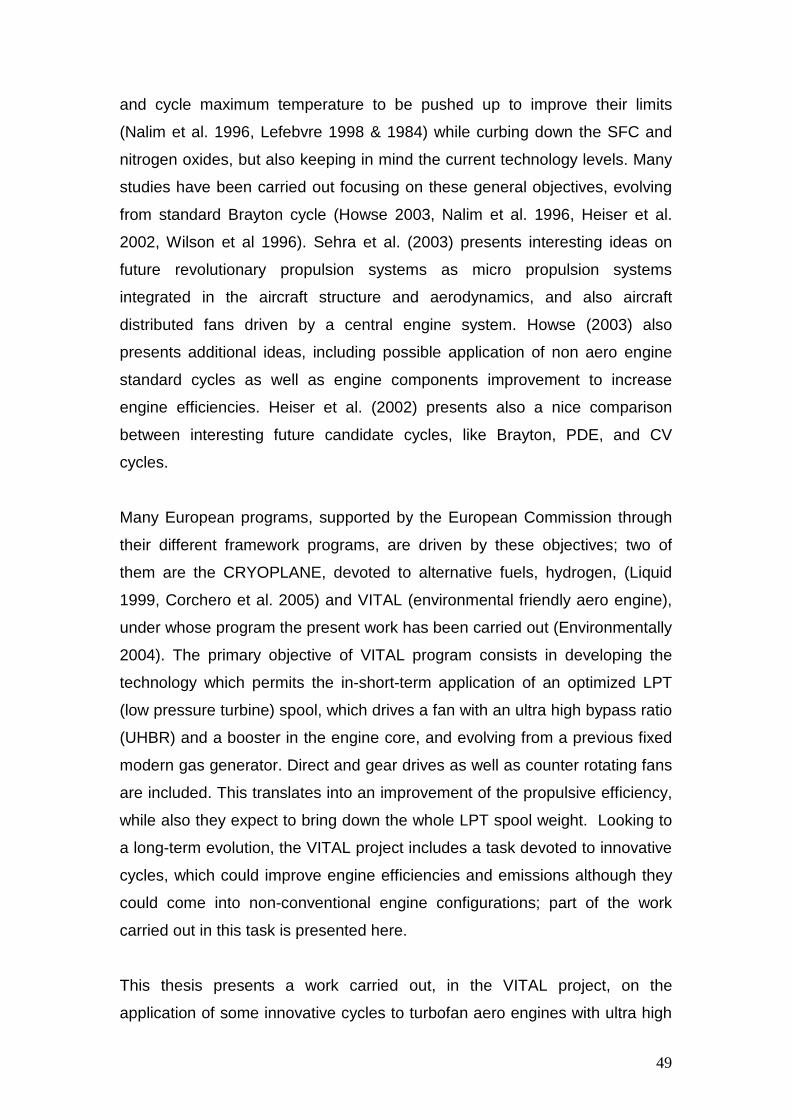
49
and cycle maximum temperature to be pushed up to improve their limits
(Nalim et al. 1996, Lefebvre 1998 & 1984) while curbing down the SFC and
nitrogen oxides, but also keeping in mind the current technology levels. Many
studies have been carried out focusing on these general objectives, evolving
from standard Brayton cycle (Howse 2003, Nalim et al. 1996, Heiser et al.
2002, Wilson et al 1996). Sehra et al. (2003) presents interesting ideas on
future revolutionary propulsion systems as micro propulsion systems
integrated in the aircraft structure and aerodynamics, and also aircraft
distributed fans driven by a central engine system. Howse (2003) also
presents additional ideas, including possible application of non aero engine
standard cycles as well as engine components improvement to increase
engine efficiencies. Heiser et al. (2002) presents also a nice comparison
between interesting future candidate cycles, like Brayton, PDE, and CV
cycles.
Many European programs, supported by the European Commission through
their different framework programs, are driven by these objectives; two of
them are the CRYOPLANE, devoted to alternative fuels, hydrogen, (Liquid
1999, Corchero et al. 2005) and VITAL (environmental friendly aero engine),
under whose program the present work has been carried out (Environmentally
2004). The primary objective of VITAL program consists in developing the
technology which permits the in-short-term application of an optimized LPT
(low pressure turbine) spool, which drives a fan with an ultra high bypass ratio
(UHBR) and a booster in the engine core, and evolving from a previous fixed
modern gas generator. Direct and gear drives as well as counter rotating fans
are included. This translates into an improvement of the propulsive efficiency,
while also they expect to bring down the whole LPT spool weight. Looking to
a long-term evolution, the VITAL project includes a task devoted to innovative
cycles, which could improve engine efficiencies and emissions although they
could come into non-conventional engine configurations; part of the work
carried out in this task is presented here.
This thesis presents a work carried out, in the VITAL project, on the
application of some innovative cycles to turbofan aero engines with ultra high

50
bypass ratios (UHBRTF), bypass ratios above twelve. Starting from the
assumption that, the LPT spool and bypass stream have been optimized to
get a maximum feasible propulsive efficiency considering the expected
technology improvement in VITAL project, different innovative cycles have
been applied to core engine to improve performances. Performances are
focused on specific thrust fuel consumption, and specific thrust improvement,
as well as on emissions, and noise levels. In this study, expected VITAL
technology level is considered as baseline technology level also.
Recently much work has been devoted to the analysis of innovative cycles,
and innovative components for aircraft propulsion systems. Sirignano et al.
(1999) and Liu (2001) present the application of inter-stage turbines
combustion and continuous turbine combustion cycles, but this cycle has not
been studied because the results show an important benefit on specific thrust,
but with an increase on specific fuel consumption due to a lower propulsive
efficiency, requiring also a new combustor-turbine technology. NASA has also
devoted much work to wave rotor simulation and development (Wilson 1993 &
1997, Welch 1997 & 1999, Paxson 1997, Nalim 1996 & 1999).
2.5 More future engine: the internal combustion wave rotor
After studying the CVC and Wave rotor separately it has been decided to do a
parametric study of an aero engine that comprises both configurations. This
engine is a blue sky concept, highly advanced and quite futuristic, with a
technology readiness level (TRL) of 7 or higher only by 2025, so only a
preliminary performance study is done, leaving to future studies the task of a
more improved analysis.
The Constant Volume Combustor (CVC) concept implements a type of
constant volume combustion process utilizing wave rotor type machinery.
Compared to a conventional turbine engine combustor, the CVC creates a
pressure rise in addition to temperature rise. This results in the potential for

51
greater work extraction from the flow through the turbine or higher pressure
available at the exhaust nozzle to produce thrust.
The machinery is like that of a wave rotor, because the CVC is a type of wave
rotor with the additional fact that the combustion takes place within the rotor
tubes. The picture below is a highly conceptual drawing of the proposed
device with each of the components labeled (Smith et al 2002). Flow enters
from the left and travels to the right.
In sequence, the flow passes through the compressor transition duct, inlet
endplate, rotor, exit endplate, and exits through the transition duct toward the
turbine. Some of the flow will transition through the buffer air ducts after
entering the rotor, through which it will then be discharged into an adjacent
tube within the rotor. Notice that there are a large number of tubes or
channels within the rotor. Identical processes take place within each tube. The
process in each tube is out of phase with that in the other tubes relative to the
angular position of the tube. Having many tubes in the rotor enhances the
quasi-steady in and-out flow. Fuel is detonated at the right end of the rotor
tube, indicated on the endplates in the picture. The rotor revolves to provide
valve action, i.e., opening and closing of ports into and out of the rotor. The
endplates have cutouts which are the ports. As the rotor spins, the tubes pass
by the cutouts in sequence for proper “opening” and “closing” of the ports.
Transition ducts at either end are required to carry flow from the partial
annulus of the wave rotor to the full annulus of the turbomachinery and to
dampen the unsteady effects of the flow entering and leaving the CVC.

52
Figure 16: CVC machinery exploded view (Smith et al 2002)
Figure 17 general arrangement of the CVC (Smith et al 2002)
A developed view of the flow processes occurring within the CVC is shown in
Figure 18, illustrated in x-t diagram form x being the distance along the tube
axially and t being time. The process sequence begins at the bottom of the
diagram where a mixture of air and fuel are trapped within the tube as the
tube translates upward (t increasing during rotor rotation) and approaches
Port 5.

53
Figure 18 developed view of the CVC process (Smith et al 2002)
The detonation of the mixture is initiated as it passes Port 5 on the exit end of
the CVC. The exact mechanisms of initiation were not modeled in detail for
the purposes of this study. Implementation will depend on applying lessons
learned in recent PDE research. The detonation then travels to the left down
the tube as the fuel is combusted. When the detonation passes out of the
region having fuel and into the region where no fuel is present, a resulting
shock wave travels toward the inlet end through the remaining air in the tube.
On the right or exit end of the tube, the opening to the duct adjoining the
downstream turbine is opened. This initiates a set of expansion waves, which
accelerate the flow within the tube and this flow exits the tube through port 6
and enters the turbine transition duct. A moment later, on the inlet end, the
portion of the flow compressed by the shock wave, exits via port 1 and enters
a short loop of duct on the inlet end of the CVC. Within this duct the high
pressure flow is turned back into the rotor, reentering the rotor some moments
later at Port 2. (Note: Some of this buffer gas can also be used for high
pressure turbine cooling, a feature previously not available with pulse
detonation combustors until fairly recently.) This reentering of high-pressure
non combusted gas is the key element to providing a uniform outflow to the
turbine inlet. Introducing this compressed gas back to the tube causes the hot
gas expansion and expulsion process in the tube to finish in an energetic
manner. The energy added by the compressed gas allows a highly uniform

54
pressure and velocity process to continue within the tube during the entire
time the hot gases are discharging.
Essentially, all packets of flow arriving at the exit have the same energy level
thus allowing a steady flow at the exit of the CVC. As the compressed gas is
reintroduced on the left end, fuel is added within Port 2. As port 2 is closed,
port 3 is opened and fresh compressor air is swept into the tube behind the
gas rushing toward the exit at the right. As the discharge port 6 is closed, a
hammer shock is formed which travels to the left compressing the incoming
flow. The tube is closed as the shock arrives at the left end of the tube. The
process is now ready to repeat.
A comparison of an advanced reference engine using conventional
turbomachinery to the current layout of a CVC based engine is shown in
Figure 19. Several differences between the engines can be noted. First of all,
conventional engine compressor is replaced with a low pressure ratio
compressor due to the pressure rise characteristic of the CVC.
Figure 19 conventional versus CVC engine (Smith et al 2002)
2.5.1 Advantages and Limitations of the Internal Combustion Wave
Rotor
Advantages:

55
Pressure gain during combustion, thanks to this the turbomachinery of
the engine can have a smaller size and lighter weight
Constant volume combustion is more efficient, because of the shock
wave system it uses.
Higher overall pressure ratio
Higher overall temperature ratio
Lower SFC, because in detonation a leaner mixture is used in order to
create the same amount of energy
Higher thermal efficiency, because of the higher temperatures
achievable with deflagrations
Steady flow at exit of ducts
Self cooling, because in the wave rotor there is always an alternation of
cold and hot flow in his tubes creating a perfect cooling environment
Can replace entire spools, because the increase of pressure and
temperature is done in the wave rotor and the combustor the HPC and
HPT are smaller
Possibility of reduced engines size and weight, again the compactness
of the wave rotor ensures that the turbomachinery can have a lower
number of stages.
Limitations:
High thermal fatigue loading, because of the high TET creep and
fatigue are a main concern

56
Structural integrity is an issue because of detonations
Combustion initiation is difficult, because the creation of detonation
under a controlled environment in not an easy task
Sealing issues are a major problem, because there is a complex valve
system connected to the closing and opening of the wave rotor’s ports
Complicated mechanism, as we can see in Figure 16 and Figure 17
this type of engine has a quite elaborated structure and it’s
manufacture would not be easy in mass production
Failure modes are unknown
Cost of production is unknown
Shock waves possibility and uncertainty of the interaction of them with
the turbine
Unsteady device makes calculation, design and analysis unpredictable
and difficult

57
3. Economic Module
In this chapter all the input and output of the economic module are explained.
Engine design decisions have significant influence on the first cost and
operating expenses. It is therefore important to understand the cost
implications of engine manufacture and operation and to take these into
account when deciding the aircraft configuration and performance.
The costs of manufacturing are calculated in the Plant cost module of TERA
(see Figure 22) and are received as an input by the economic module, so they
are not considered here.
Consideration of cost aspects is especially significant in the preliminary
design phase of engine projects as fundamental decisions are taken which
will be influential in the overall cost of the project. Such decisions affect the
cost of manufacturing and equipping the basic engine and the subsequent
cost of operating it over the route structure of an airline. It is therefore
essential to understand the cost estimation methods to be used by the
customer when comparing competitive engines, in order to make sensible
design choices.
Here are introduced the methods by which engine operating costs are
estimated. These methods are used in the preliminary project phase to allow
comparisons to be made between different aircraft configurations and to
assess the best choice of values for all the aircraft parameters.
Indirect costs (those not directly related to the engine parameters, for example
those associated with marketing and sales expenses) are not covered,
whereas direct costs are described in enough detail to allow estimating
methods to be incorporated into the aircraft design process. The principal cost
functions are described and typical values given.

58
A comparison between my model, a model created by Roskam (1990) and
values taken from magazines for the A330-200, the A320-200 and different
types of long and short range engines is presented.
Engine project designers are seen to influence costs directly by the basic
configuration of the engine (system complexity, aircraft size, engine size, etc.)
and selected performance (cruise speed, range, etc.). All these aspects will
have a substantial input to the cost model through the standing charges, the
fuel used and the maintenance required. The designers also influence cost
indirectly through airline economics (market size, ticket price, engine
performance, passenger appeal). These indirect factors feed into the cost
analysis through revenue potential, the demand for the aircraft type, market
development and ultimately to commonality and type derivations. It is
important for the designers to recognise these influences in the early stages
of the engine project so that the design can meet the market potential and
thereby maximise success of the project.
3.1 Methodology
Under the direct operate cost (DOC) category all the costs associated with
flying and direct maintenance must be considered. The cost components may
be considered in three broad headings:
Standing charges
Flight costs
Maintenance costs
A description of each of these headings is given below in Figure 20.

59
Airframe cost Engine cost Avionics cost Loans cost
Aircraft cost Spares cost
Total a ircraft price
Insurance rate
Interest rate
Insurance cost
Loan payments
Maintenance cost
Airframe cost
Engine cost
Crew cost
Fuel/oil cost
Airport fees
Flight operation cost
Total direct operating
Cost (DOC)
Figure 20 Direct operating cost (DOC) components (Jenkinson 1999)
Standing charges:
These are the proportion of the costs that are not directly linked to the engine
flight but may be regarded as ‘overhead’ on the flight. Such costs, in order of
importance, include:
Interest charges on capital employed
Engine insurance
Interest charges are impossible to quantify in a general analysis as the banks
and government agencies will charge different fees to different customers.
Such charges will be dependent on the world economic climate, local
exchange rates, the credit standing of the purchaser and the export
encouragement given by the national government of the airline or the
manufacturer. Usually current national base interest rates should be used to
account for this type of cost.

60
The insurance cost is directly related to the risks involved and the potential for
claims following loss. Insurance companies will vary their fee in relation to the
nature of the operation and the level of airline security. The fees vary usually
between 1 and 3% of aircraft value.
Flight costs
This cost element comprises all the costs which are directly associated with
the flight. They are:
Fuel and oil usage
Airport charges
Included in the airport charges are not only the landing and navigational fees
but also the taxes on noise and emissions that nowadays are becoming more
and more important due to the concern about environmental pollution from the
public and government alike.
Maintenance costs
Prediction of maintenance costs is complicated by the lack of definition for
items to be included under this heading. Setting up a maintenance facility is
an expensive outlay for the airline. Some such facilities run as a separate
business. The capital cost of building, the administration costs and the cost of
special equipment may be regarded as an indirect cost on the total
maintenance operation and included in the Indirect Operating Cost evaluation.
These suits the aircraft manufacturer as the evaluation of DOC would
proportionally reduce.
Maintenance charges include labour and material costs associated with
routine inspections, servicing and overhaul. The equations used for calculate
the maintenance costs are shown in annex F.
In an inflationary economic climate, values for costs are highly time-
dependent; therefore some effort must be made to secure current prices for

61
the various elements that make up the total operating cost. Alternatively, old
prices must be ‘factored’ to account for changes since publication. This
factoring requires the use of an inflation index. This index has been applied to
most of the costs already described.
The economic module has inside a lifing module to study the lifing of rotor
blades and the disk of the high pressure turbine. It is important because the
maintenance costs depend strongly on the time between overhauls of the
components of the engine and the high pressure turbine has the most severe
operating environment of all the parts of the engine.
To the lifing module the Weibull distribution is applied in order to generalise
the lifing prediction taking into account all the parts of the engine which can
cause breakdown.
The Risk Module
The economic module has also a risk module inside in order to do a Monte
Carlo Risk Analysis for the DOC over a period of time of thirty years, which is
considered the average life for both the aircraft and the engine. An
explanation of the Monte Carlo Method has been done in paragraph 2.2.
The risk model uses Gaussian distributions applied to several parameters that
affect the DOC and NPC like:
Interest Percentage
Fuel Price
NOx
Downtime
Inflation
Labour
Carbon Tax
Noise Tax
Time Between Overhaul

62
The risk is applied to 10000 scenarios, this number of scenarios is considered
in statistic evaluation as the minimal required in order of being sure that the
analysis has a meaning, and then a classical S shaped cumulative curve is
created, as we can see in Figure 21Figure 34.
NET PRESENT COST DISTRIBUTION
0
20
40
60
80
100
120
9974
10182
10390
10598
10806
1101
4
1122
2
11430
11638
1184
6
12054
NPC (K€)
CU
MU
LA
TIV
E
FR
EQ
UE
NC
Y(%
)
Figure 21 Cumulative curve for the net present cost (NPC)
The economic module has to be integrated with other modules like an aircraft
module and a performance module created here in Cranfield, a weight module
done by Chalmers University in Sweden, a plant cost module done in Stuttgart
University and two modules that analyse the noise and emissions done in
SUPAERO University in France. This integrated complex system is called
TERA: Thermo Economic and Risk Analysis. The integration of these entire
modules is done through a licensed program used by many industries called
iSight. This is a very powerful tool that can do optimization, design of
experiment, trade-off analysis, optimum robust design and approximation
methods. Thanks to TERA the VITAL project will be able to create optimal
design of engines with a good trade-off between performance and costs.

Figure 22: the TERA structure (TERA 2006)
Directory: Econo
EcoModu eInpudat
m
performanceResultstxt
Engine_Var dat engine_dp dat AcMissonProf le txt
2Files
File
EngEmissonDatadat
TmatchCalls exe
performanceAircrafttxt
TERAflghtemissionProfe dat
EngAcData txt
Directory: Performance
Directory: Emissions
Directory: Aircraft
CombustorData dat
AcFl ghtPathRes txt
weight~ utp ut txt
Hermes exe
EmissionsModule exe
engine_$ital dat
engine dat
AcGeomMissionSpec txt
TERAemissonsOUTPUT dat
Parameter and Boundary Conditions in ISIGHT
AcF ghPathFuelCons umption txt
performanceWeighttxt
we ghtAircraft txt
TURBOMATCH exe
Weico exe
dmensionsWeighttxt
weightDOC txt
Directory: WeiCo
Directory: Noise
TERAnoiseINPUTdat
software interface(windows dll)
weghtNoiseEmssions txt
material_databasetxt
EngNoiseData dat
TERAnoseOUTPUT dat
NoiseModule exe
P antCostResuts fo
Saecc/nput ec(optional)
saecc dll
SopranoData dat
SopranoMain exe
' Fi leso F l
o F leSoprano
Data s
t
ics
ba
haring by
de_stress_inputdat
EcoModultxt
exchanging file
stand'o prano
temporary
eO
s
disc_input dat ndat_creep dat Indat_fati3ue dat
Directory: Environmental
AircraftEmissons txt
utp
Eco
ut
Module ex
N
e CGWPD exe
pcO utp
Data s
ut
h
tx
a
rt
ing
th ro ugh ISIGHTTERA R
esults in IS IGHTC
G WPDOutpu t txtTERA A
o pr a
'opra Files
natomy Version 8 0

64
3.2 Economic Module Description
In this section, a description of the Economic module is given. The features of
the economic module are based on the TERA high level specification given by
the VITAL project. The capabilities of this current version of the Economic
module would be shown via the inclusion of the input file and examples of the
program outputs. The programming language for the economic model is Fortran
90.
3.2.1 Economic Module Architecture
The flow chart with the architecture of the economic module is shown in the
figure 23:
Figure 23 Economic Module Structure
3.2.2 Module Requirement Definition
A set of requirements was developed and implemented into the economic
module. These include the following capability to vary as inputs:
Cost of aviation fuel
Cost of maintenance hours
Interest rates
Noise charges at airports
Carbon emission charges
Lifing Module
Economic Module
Risk Module

65
NOx charges
The Risk Module
Also a stochastic risk module, developed following the Monte Carlo approach is
integrated into the economic model. This enable scenario studies with the input
parameters taking likely distributions and the analysis conducted over the
product life.
Through the selection of variables in the input file it is possible to choose which
variables will be changed by the risk module. If the value of the selector is 1 the
variable is not changed by the module, with a value of 2 the module will change
the value of the variable. The values that are not changed by the module have
to be given by the user in the input file. The risk requires the minimum and
maximum of the variables that it has to change.
If the economic program has to work without the risk analysis, N (number of
scenarios studied by the program) has to be set to 1. With a value of N>1 the
economic analysis will use the risk module.
The NOX factor B is a variable that increases the value of NOX considering the
future increase of the tax.
The Noise tax is calculated using a threshold system of taxation. A value for the
threshold is given in input and if the noise produced by the engine is higher than
the threshold, the higher is the tax. The same policy has been used for the
Carbon Tax.
3.2.3 Input file Definition
Some key parameters required by the economic model and their sources (other
modules that are in TERA) are shown in the table 3:

66
Parameter Source/Module
Cost of aviation fuel (c$/US gallons) User defined
Cost of flight and cabin crew (€/FH) User defined
Cost of maintenance hours (€/FH) User defined
Interest rate (%) User defined
Noise level (dB) Noise model
Emission level Emissions module
Block fuel (kg) Ac Performance module
Block time (hrs) Ac Performance module
Shaft speed (relative) Engine performance module
TET (k) Engine performance module
Plant cost (k€) Plant cost module
Table 3: Key Economic Module Parameters
The typical input file for the economic model is a notebook file that requires data
for the engine and the aircraft.
It incorporates data that are used by both the economic and risk modules.
It has several parameters, but the most important are:
Take off Thrust: from this depend the maintenance hours needed by the
engine.
Overall Empty Weight: to assess the maintenance hours needed by the
airframe.
Weight of Fuel Used.
Time between engine overhaul: this parameter can be given by the user
or can be calculated by the lifing module.
All the elements needed to calculate the airport fee and taxes, like noise
and emissions.
The input file for the lifing module (blade_stress_input.dat, disc_input.dat,
indat_creep.dat, Indat_fatigue.dat, material_database.txt) contains the data
needed to calculate the creep and low cycle fatigue from an analysis of the

67
stresses for the blades and the disk of the high pressure turbine, which is
typically the most life limited component.
In order to calculate creep and fatigue several geometrical parameters and the
properties of the materials used in the components are needed, such as the
Larson-miller parameters, for the creep, and the coefficients of the Coffin-
Manson equation, for the low cycle fatigue.
Also needed are the temperatures and duration to which the components are
exposed during the flight cycle. The lifing module will be better explained in the
next section.
3.2.4 Output Files
Amongst the outputs the economic model would give are:
Direct operating cost, DOC (k€)
Engine maintenance cost (k€)
Net present cost, NPC (k€).
Cost of taxes (k€)
Stresses of the blades and the disk.
The cost of labour and materials used in the overhaul.
The NPC is obtained over a time frame defined by the user to depict the engine
operating life.
The cumulative curve enables the planners to assess risk when a specific
minimum value of NPC is targeted. In such conditions, if the airline plans to
spend 11.5 millions of Euros the NPC value is 80%, so the risk estimated is
20% as we can see from Figure 21.

68
3.3 The lifing Module
The lifing module has been done by the master student Oliviero Vigna Suria
and integrated by the author in the economic module with little modifications.
The general theory behind the lifing analysis has been explained in paragraph
2.1.4. The results that validate the module can be found in Vigna Suria’s thesis
(2006).
Oxidation and hot corrosion, creep, thermal mechanical fatigue can all
potentially lead to turbine hot section component failure. Assessing gas turbine
blade life is a multi-disciplinary task requiring expertise in metallurgy, material,
mechanical design, fracture mechanics, aero-thermal dynamics, combined with
operation and service history. The life limits provided by original equipment
manufacturer (OEM) are calculated on the basis of a design envelope of
expected base load, calculated or measured component stresses and
temperatures as a function of operating conditions, expected response of the
material to those conditions, and safety factors to take into account
uncertainties in the model and natural variability of the materials. Because of
uncertainties in each of these factors and variations between the operating
conditions of specific engines, the OEM estimated life may be too conservative
in some instance, while in others, the OEM design life may not be achieved.
Conventional maintenance scheduling techniques are typically based on the
OEM’s guidelines and applied to all engines of a certain make and model. This
approach does not always address the specific operating environment and
requirements of each operator.
Using the basic failure theories, together with a stress analysis depending upon
the operating conditions, explained in paragraph 2.1.4, the lifing module is able
to determine with certain accuracy the time between engine overhaul, taking
into account every kind of uncertainty through what are known as ‘safety’ or
‘ignorance’ factors.

69
3.3.1 Structure of the lifing module
The module has been written in Fortran 90 language.
Blade StressAnalysis Module
Disc Stress AnalysisModule
Coolingsubmodule
Creep AnalysisModule
Main Lifing Model
MaterialProperties
Low Cycle FatigueAnalysis Module
Performances andoperating settings
Blade StressAnalysis Module
Disc Stress AnalysisModule
Coolingsubmodule
Creep AnalysisModule
Main Lifing Model
MaterialProperties
Low Cycle FatigueAnalysis Module
Performances andoperating settings
Blade StressAnalysis Module
Blade StressAnalysis Module
Disc Stress AnalysisModule
Disc Stress AnalysisModule
Coolingsubmodule
Coolingsubmodule
Creep AnalysisModule
Creep AnalysisModule
Main Lifing ModelMain Lifing Model
MaterialPropertiesMaterial
Properties
Low Cycle FatigueAnalysis Module
Low Cycle FatigueAnalysis Module
Performances andoperating settingsPerformances andoperating settings
Figure 24, Lifing Module Breakdown (Vigna Suria 2006)
Knowing the maximum stress acting on the blades and on the disc, plus some
additional settings and performance data (i.e. time spent and TET, that will
allow to define the actual scenario, in terms of stress-time-temperature), the
creep module will calculate the creep life time for both the components, as
normally they are made from different materials, thus having a different life time.
On the other hand, using simply the material’s properties and the peak of
temperature experienced when starting-up the engine, the low cycle fatigue
module will estimate the fatigue lives.
The main algorithm will then compare creep and low cycle fatigue life times: the
lower will be considered as the real time between engine overhaul, and passed
to the economic module as an input.
The important facility offered by the module is the possibility to run either the
module as a whole, or each module independently, depending on the amount of
information available when running the algorithm.

70
All the uncertainties can be taken into account by the use of what are known as
‘safety’ or ‘ignorance’ factors, available in the code.
An important issue that has to be pointed out is how creep and low cycle fatigue
affect the life time of the engine’s HP turbine during each type of mission, since
the failure mechanism that gives the lowest life, will be the one to adopt in
predicting time between engine overhaul.
In Figure 25, the influence of both creep and fatigue can be appreciated as a
comparison between the relative importance’s they have.
0
10
20
30
40
50
60
70
80
90
short range medium range long range
Nu
mb
er
of
Fa
lure
s(%
)
creep
fatigue
Figure 25 Creep and Low cycle fatigue life for different types of mission
The results show the presence of a predominant failure mechanism for both
short and long range (the exact amount of hours has not been reported on the y
axis, since this is just a relative comparison, not aiming at giving any real result
but only the trends). In particular, short range missions are dominated by low
cycle fatigue failure, due to the high amount of start-stop cycles the engine is
subject; on the other hand, long range engines are affected mainly by creep
failure, since the fraction of time spent at elevated temperature is significantly
high, thus allowing creep to act intensively on the component.
For medium range aircrafts, the situation is more or less balanced, with the two
failure mechanisms influencing the life time more or less in the same
percentage.

71
3.3.1 STRESS ANALYSIS
First in the lifing model comes the stress analysis. Different approaches are
available, as the code is user-friendly, and allows the user himself to choose
among different levels of details through the use of selectors to be set
appropriately in the input file.
Two different subroutines have been carried out: the first one estimates the
stresses acting on the turbine’s blades, while the second one analyses the disc.
3.3.1.1 Blade stress analysis module
The blade stress analysis module is based on the simple equations mentioned
in paragraph 2.1.4.1, it has been created by the master student Oliviero Vigna
Suria and the validation of the method can be found in his thesis (Suria 2006). It
aims to estimate the maximum stress acting on the HP turbine blades. The
code itself is in appendix F.7.
The flow chart in Figure 26 shows the module breakdown.
Input Radius and crossarea of each section
Input Material data(density), and RPM
Input Number of bladesections
MAXIMUM STRESS ON THE BLADE
Centrifugal load and stress for each section
Input Radius and crossarea of each section
Input Radius and crossarea of each section
Input Material data(density), and RPMInput Material data(density), and RPM
Input Number of bladesections
Input Number of bladesections
MAXIMUM STRESS ON THE BLADEMAXIMUM STRESS ON THE BLADE
Centrifugal load and stress for each sectionCentrifugal load and stress for each sectionCentrifugal load and stress for each section
Figure 26 Blade stress module structure (Vigna Suria 2006)
Entering into a detailed description of the code itself, the subroutine is called
from the main program, giving an input, namely the HP spool speed in RPM,
and getting an output, that is the maximum stress acting on the blade.

72
An input file in the form of data sheet (blade_stress_input.dat) is required and
showed in Appendix A; the following are the most important inputs:
radius
cross sectional area
By knowing all these data, and applying the stresses equations, the code
estimates the centrifugal stresses acting on each section of the blade, and
subsequently the maximum stress acting at the blade root.
3.3.1.2 Disc stress analysis module
The disc stress analysis module, which aims at calculating the maximum stress
acting on the HP turbine disc, it has been created by the master student Oliviero
Vigna Suria and the validation of the method can be found in his thesis (Suria
2006). The code itself is in appendix F.6.
The structure of the module is reported as a flow chart in Figure 27.
Input RPM, Material data(density, Poisson’s ratio)
Constant orvarying thickness
disc?
Rim stress is alreadyknown or not?
Equivalent Von Mises stress
MAXIMUM STRESS ON THE DISC
Constant Varying
NO
YES
YES
Rim stress calculated = to theknown one?
NO
Input rim and bore diameter,and disc thickness
YES
NO
Call blade stresssubroutine to get the rim
stress
Bore and rim radial andhoop stress calculated
Call blade stresssubroutine to get the rim
stress
Input number of ring, withtheir radius and thickness
Rim stress is alreadyknown or not?
Bore hoop stress guessed, Radialand hoop stresses at the bore and
the rim calculated
Input RPM, Material data(density, Poisson’s ratio)Input RPM, Material data(density, Poisson’s ratio)
Constant orvarying thickness
disc?
Constant orvarying thickness
disc?
Rim stress is alreadyknown or not?
Rim stress is alreadyknown or not?
Equivalent Von Mises stressEquivalent Von Mises stress
MAXIMUM STRESS ON THE DISCMAXIMUM STRESS ON THE DISC
Constant Varying
NO
YES
YES
Rim stress calculated = to theknown one?
NO
Input rim and bore diameter,and disc thickness
Input rim and bore diameter,and disc thickness
YES
NO
Call blade stresssubroutine to get the rim
stress
Call blade stresssubroutine to get the rim
stress
Bore and rim radial andhoop stress calculated
Bore and rim radial andhoop stress calculated
Call blade stresssubroutine to get the rim
stress
Call blade stresssubroutine to get the rim
stress
Input number of ring, withtheir radius and thicknessInput number of ring, withtheir radius and thickness
Rim stress is alreadyknown or not?
Rim stress is alreadyknown or not?
Bore hoop stress guessed, Radialand hoop stresses at the bore and
the rim calculated
Bore hoop stress guessed, Radialand hoop stresses at the bore and
the rim calculated
Figure 27 Disc stress module structure (Vigna Suria 2006)

73
As for the blade stress subroutine, also this one is called directly from the main
program, giving the same input, namely the HP spool speed in RPM, and
getting the maximum stress acting on the disc as output.
Again an input file in the form of data sheet (disc_input.dat) is required and
showed in Appendix A, where the following details have to be specified by the
user:
a check to determine whether the disc is a constant or a varying
thickness disc;
Another check to define whether the rim stress due to the blades that the
disc is carrying will be provided by the user or will have to be calculated.
In case of a constant thickness disc, the rim diameter, the bore diameter, and
the thickness of disc have to be inserted as input, together with either the rim
stress, if it is given as an input, or details regarding the blades (namely number
of blades, blade mass and radius of the centre of gravity of the blades, given
with respect to the blade root), if it has to be calculated.
If the disc has a variable thickness, the approach is different: the disc has to be
split into several rings, each one being considered as a constant thickness ring.
The last step is to compare the estimated value of the rim stress, with the real
one due to the presence of the blades the disc is carrying, and to proceed
iteratively adjusting the bore hoop stress, until the calculated rim stress will be
the same as the real one.
Again, after getting the right radial and hoop stress across the disc, they will be
combined through the use of Von Mises equation in order to get the equivalent
stress acting on each ring, thus being able to find the maximum stress acting on
the disc.

74
3.3.2 Application of cooling within the code
Both creep and low cycle fatigue algorithm include a fairly simple blade cooling
system. The process is based on a certain amount of air spilled from the last
stages of the HP compressor, just before entering the combustor, and
transferred to the HP turbine, where it will cool the blades.
In the structure of the fairly simple blade cooling sub-module can be
appreciated. The module follows the equations and assumptions done in
paragraph 2.1.4.2. The module has been tested and created by the master
student Oliviero Vigna Suria and the validation of the method can be found in
his thesis (Suria 2006). The code itself is in appendix F.5.
Figure 28 Blade cooling sub-module structure. (Vigna Suria 2006)
For simplicity of purposes, the model starts from a defined value of overall
effectiveness that the user has to input, avoiding all the calculations involving all
the other parameters mentioned in paragraph 2.1.4.2, since it is assumed that
the engine designer will provide the exact amount of air needed to get such an
effectiveness; moreover, the main point of the algorithm is to estimate the new
temperature of the cooled blade, rather than focusing on the blade cooling
system.
Hence, knowing the temperature of the coolant entering the blades (i.e. the
temperature of the air leaving the HP compressor), the temperature of the gas
surrounding the blades (TET) and the effectiveness being inputted by the user,
very easily the code provides the new temperatures of the component. After
that, the main algorithm (both the creep and the low cycle fatigue analysis)
proceeds normally, as it will be explained in the next two chapters.
Input T blade, T coolant and cooling effectiveness
NEW Temp BLADE CALCULATED

75
3.3.3 Low cycle fatigue module
As mentioned in the previous paragraph, although most engineering structures
and components are designed such that the nominal loads remain elastic,
thermal stresses due to high peaks of temperature (as it is for the HP turbine of
an engine) often cause plastic strains to develop. Due to the constraint imposed
by the elastically-stressed material surrounding the plastic zone, deformation is
considered strain-controlled.
The module is able to predict the low cycle fatigue of an engine component,
using the theory explained in paragraph 2.1.4.5, the Coffin–Manson rule,
together with the Neuber method applied to cyclic loading, explained later in the
paragraph.
It has been created by the master student Oliviero Vigna Suria and the
validation of the method can be found in his thesis (Vigna Suria 2006). The
code itself is in appendix F.4.
In particular, this method is a strain method, based on the capability of which
the material component is made from to tolerate the start-stop cycle it is subject
every time it is started and ready for the take-off, that is the most critical
moment for the turbine, as it experiences the peak of TET.
The purpose is to determine the fatigue life of the component loaded with
thermal stresses arising from the temperature difference due to the engines
starting, namely the difference between the TET and the ambient temperature.
The breakdown of the low cycle fatigue module is reported in the Figure 29:

76
Input T amb andmax TET
Strain range calculation(Neuber method)
Guess number of cyclesto failure, and
calculate strain rangewith MUS
MUS Strainrange =
Neuber Strainrange?
NUMBER OF CYCLESTO FAILURE
YES
NO
Input T amb andmax TET
Input T amb andmax TET
Strain range calculation(Neuber method)
Strain range calculation(Neuber method)
Guess number of cyclesto failure, and
calculate strain rangewith MUS
Guess number of cyclesto failure, and
calculate strain rangewith MUS
MUS Strainrange =
Neuber Strainrange?
MUS Strainrange =
Neuber Strainrange?
NUMBER OF CYCLESTO FAILURE
NUMBER OF CYCLESTO FAILURE
YES
NO
Figure 29 Low Cycle Fatigue module structure (Vigna Suria 2006)
Knowing the linear coefficient of thermal expansion of the material the
component is made from, and assuming a perfect elastic behaviour of the
material itself, the maximum thermal strain and the maximum associated stress
can be estimated, the former simply by multiplying the ∆T by the linear
coefficient of thermal expansion itself, the latter by multiplying the thermal strain
by the elastic modulus of the material.
The Neuber Rule
In reality, when the yield stress of the material is overtaken, the component
starts deforming plastically, following its stress-strain curve. The Neuber rule
(derived for determining the strain distribution around a notch) allows
determining the strain that occurs at the yield stress, by identifying a hyperbola
on the σ-ε diagram, that is:
.const
The product between the maximum thermal stress and strain just calculated will
define the value of the Neuber constant, through which it is possible to proceed
estimating the strain that actually occurs at the yield stress, simply by dividing
the Neuber constant by the material yield stress.

77
When the unloading part of the cycle occurs, the stress range returns along the
elastic straight line of the σ-ε diagram, unless the yield limit in compression is
reached.
For the compressive phase, a new Neuber hyperbola has to be found, because
there will be the same problem of the specimen behaving plastically rather than
totally elastic. That means that the unloading phase, which started at the tensile
yield stress, will last until the maximum thermal stress that loaded the
component will completely be unloaded (i.e. until a stress equal to the
difference between the yield stress and the maximum thermal stress will be
reached).
Hence the maximum compressive strain can be calculated, by dividing the
maximum compressive stress (just estimated as difference between the yield
stress and the maximum thermal stress) by the elastic modulus of the material.
By multiplying the maximum compressive stress and strain together, the new
Neuber’s constant is defined, thus being able to determine the compressive
strain corresponding to the compressive yield stress.
Now that all the needed figures are known, it is possible to calculate the total
strain range εT as difference between the tensile and the compressive strains,
and to proceed with the final step, namely the estimate of the number of cycles
to failure, by applying the MUS. The solution will be found iteratively, as the
procedure is to guess the number of cycles, thus getting a value of total strain
range that will be compared with the real one, calculated before through the
Neuber rule: the iterations stop when the difference between the real and the
estimated value of total strain stays within 1%.
As in the creep algorithm, even in the low cycle fatigue algorithm, the user has
the possibility to choose among three different analyses:
only the blade;
only the disc;

78
disc and blade together
3.3.4 Creep module
The creep algorithm is able to estimate the creep life of an engine component,
applying the Larson-Miller parameter criterion, together with the Miner’s
cumulative creep law, as explained in the background theory in the previous
pages.
It has been created by the master student Oliviero Vigna Suria and the
validation of the method can be found in his thesis (Vigna Suria 2006). The
code itself is in appendix F.5.
The flight envelope has to be split into several segments (e.g. climb, cruise and
descent), each one characterized by a time length, and a well defined operating
condition, that is a determined engine RPM, and TET. Knowing the turbine entry
temperature, and the amount of time spent during each phase, the creep life
can be estimated running the algorithm.
In Figure 30, the flow chart with the structure of the creep module is drawn.

79
Input number ofsegment of flight
envelope toanalyse
Max stressacting in each
segmentknown?
CREEP LIFEESTIMATE
(MINER’S LAW)
Input LMP curveby point to beinterpolated
Get the LMP foreach segmentfrom the curve
Input time and Tfor each segment
Input RPM and callstress subroutines
LMP for eachstress condition
known?
Calculation oftime to failure for
each segment
Input LMP foreach segment
YES NO
YES NO
Input time,stress and T foreach segment
Input number ofsegment of flight
envelope toanalyse
Input number ofsegment of flight
envelope toanalyse
Max stressacting in each
segmentknown?
Max stressacting in each
segmentknown?
CREEP LIFEESTIMATE
(MINER’S LAW)
CREEP LIFEESTIMATE
(MINER’S LAW)
Input LMP curveby point to beinterpolated
Input LMP curveby point to beinterpolated
Get the LMP foreach segmentfrom the curve
Get the LMP foreach segmentfrom the curve
Input time and Tfor each segmentInput time and Tfor each segment
Input RPM and callstress subroutines
Input RPM and callstress subroutines
LMP for eachstress condition
known?
LMP for eachstress condition
known?
Calculation oftime to failure for
each segment
Calculation oftime to failure for
each segment
Input LMP foreach segmentInput LMP foreach segment
YES NO
YES NO
Input time,stress and T foreach segment
Input time,stress and T foreach segment
Figure 30 Creep module structure (Vigna Suria 2006)
In particular, as mentioned before, creep is a function of stress, temperature
and time; hence the first step will be the estimate of the stress acting on the
blade and the disc, thank to the two stress subroutines that need the RPM as
unique input. A matrix is created, containing stress, temperature and time spent
for each flight segment (time can be inputted as hours of flight or percentage of
the whole flight cycle).
The creep algorithm also gives to the user the possibility of cooling the blade,
thus lowering the TET and increasing significantly the life of the component.
Once the time-stress-temperature matrix has been generated, it is possible to
proceed with the research of the appropriate Larson-Miller parameter for each
phase: in doing so, two different ways are available, namely inserting either
directly the parameters (if they are already known) or the Larson-Miller curve for
the material the component is made from, the latter being a bit more
complicated, since the user has to provide the curve in the form of several

80
known points (at least six, in order to be quite accurate), that the code will
subsequently interpolate in order to find the corresponding value for each of the
stresses acting during the flight envelope.
The code offers to the user the possibility to choose among the analysis and the
estimate of the creep life for blades, disc or both of them together.
The last step is the calculation of creep life (either in hour of flight, or in cycles,
depending on the user’s will), through the use of Miner’s cumulative creep law,
after having estimated the times to failure of each segment.
In estimating the creep life of a component, take-off and approach phases are
considered negligible, thus being not taken into account, as the amount of time
spent for each of these two flight segment is definitely low if compared to the
time length of each of the other phases. Moreover, it is difficult to simulate and
achieve accurate data of the engine for these two sections.
For the other segments, several check points will be calculated, in each point a
blade metal temperature and blade centrifugal stress will be estimated in line
with the operating conditions taken from the engine simulation. For each point
an operation time will be assigned and with the two previous variables, stress
and temperature, by the use of the Larson Miller parameter the time to failure
will be calculated.

81
4. Advanced Propulsion Systems
The work presented in this section has been conducted in the Universidad
Politecnica de Madrid (UPM) under the supervision of Prof. Gregorio Corchero
Diaz. The program used to analyze the advanced cycle has been created in
UPM and is property of UPM University.
4.1 Candidate Cycles Description
Three cycles have received especial attention for their application to turbojets
during last years. All of them are based on the application of some modifications
to the standard Brayton cycle to get a higher efficiency by introducing new
components. These cycles are:
a) intercooler-regenerative cycle (IRC)
b) The wave rotor topping cycle (WRTC)
c) The PDE (pulse detonation engine) and the CV (constant volume) cycle or
Humphrey cycle, which really represents a first approximation to the PDE cycle
(Heiser 2002).
This section will be devoted to the study of these three cycles, searching for a
performance improvement when they are applied to a next generation turbofan
engines as VITAL engines are expected to be. The work will be based on their
possible benefits on SFC, ST, emissions, and noise level as well as on the
technological level required. Next paragraphs present a brief description of each
one.
IRC cycle:
In this cycle the intercooler (IC), a heat exchanger, cools the mass flow coming
into the high pressure compressor (HPC) transferring energy from the core
engine stream to the bypass stream at the exit of the outer fan, see Figure 31.

82
This saves energy in the compression process, improving also the bypass
contribution to the engine specific thrust, but it will need additional fuel to get a
given temperature at the exit of the combustor. This increase of fuel is
compensated by an energy transfer from the exit of the LPT to the entrance of
the combustor, the regenerative heat exchanger (RHE), while the mechanical
energy available at the exit of the LPT decreases smoothly producing an
increase of thermal efficiency. It is a typical application in sea and terrestrial
power generation (Saravanamamutto 2001, Sawyer et al. 1972, Dellenback
2002, Beck 1996, Bhargava et al. 2004), and in other special applications
(Martinez-Friaz et al. 2004, Barret 2005). Some works can be found on IRC
application to aero engine, especially in international symposium and including
the development of heat exchangers for aero engine applications (Missirlis et al.
2005, Yakinthos et al. 2006). Finally NEWAC (new aero engine core concept) is
also a European project devoted to the development of these technologies
(NEWAC 2006).
Figure 31 the Intercooled Recuperated Cycle

83
The WRTC:
Wave rotors are devices which use unsteady waves to compress and expand
air in a single device. The wave rotor consists in a duct or multiple ducts, near
parallel to the rotating axe, surrounded at the ends by a stationary casing; the
casing end walls are penetrated by inlet and outlet ports that carry gas to and
from the rotor passages or ducts. At any time sectors of the rotor flow annuli are
exposed to the ported flow while the remaining sectors face the casing end
walls (Paxson 1996, Welch 1997). At the inlet port, low-pressure gas in the rotor
passage is exposed to the high pressure port flow; a compression wave
compresses the passage gas and, thus, allows the incoming gas to enter the
rotor. At the exhaust port, high pressure-passage gas is suddenly exposed to
low-pressure exhaust port flow; an expansion wave propagates into the rotor
passage, reduces the passage pressure, and discharges the passage gas into
the exhaust port. The air, coming from the compressor, flows into the passage
on the wave rotor where it is compressed by compression waves and shock
waves, then it leaves the wave rotor passing to the combustor (CC). From
combustor, the hot gas returns to the wave rotor and expands out to a lower
pressure; passing trough the wave rotor, the gases are first compressed and
then expanded. Thus a wave rotor combines in a single device the functions
performed by a compressor and a turbine in a high spool, see Figure 32. Also,
since the wave rotor is washed alternatively by cool air from compressor and
hot combustion gases it is self-cooled, and permits the increase of the upper
cycle pressure and temperature improving thermal efficiency. NASA paid much
attention to the wave rotor for aero engine applications in the nineties, including
the design of demonstrators (Welch 1999). Also during last years much work
has been devoted to wave rotor studies (Paxson 1996 & 1999, Welch 1997,
Nagashima et al. 2007, Resler et al. 1994).
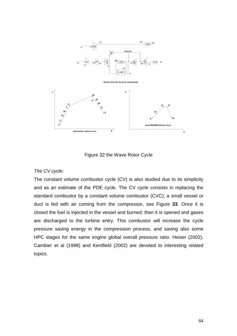
84
Figure 32 the Wave Rotor Cycle
The CV cycle:
The constant volume combustor cycle (CV) is also studied due to its simplicity
and as an estimate of the PDE cycle. The CV cycle consists in replacing the
standard combustor by a constant volume combustor (CVC); a small vessel or
duct is fed with air coming from the compressor, see Figure 33. Once it is
closed the fuel is injected in the vessel and burned; then it is opened and gases
are discharged to the turbine entry. This combustor will increase the cycle
pressure saving energy in the compression process, and saving also some
HPC stages for the same engine global overall pressure ratio. Heiser (2002),
Cambier et al (1998) and Kentfield (2002) are devoted to interesting related
topics.

85
Figure 33 the Constant Volume Combustion Cycle
The emissions are important drivers in aero engines design and use. This
section presents a part of the work carried out in the VITAL project; it consists in
a parameter study on the application of three innovative thermodynamic cycles
to aircraft propulsion looking for benefits on fuel consumption, carbon dioxide,
nitrogen oxides, and noise. These cycles are the intercooler-regenerative, the
wave rotor topping, and the constant volume combustor cycles. The work,
starting from a next generation ultra high bypass ratio turbofan, the baseline,
and considering two possible design conditions, presents the influence of the
application of these new cycles or design changes to the baseline on the
emissions and the required technological level, represented by turbine entry
temperature (TET). The baseline is a representative ultra high bypass ratio
turbofan in the VITAL project. The results show that some significant benefits on
emissions can be achieved although they are linked to significant technology
improvements and in-depth studies of the new components, involved in the
cycle implementation.

86
4.2 Performance model
The study uses has baseline engine the long range GTF (gear turbofan) engine,
it has been done at the design point of Top of Climb ISA+10, 10668 m. and
M0=0.82 and at the off design point of Cruise (10668 m. and M0=0.82); hereafter
this engine will be referred as baseline engine, and its values at the respective
flight conditions will represent the reference values in this work. Similar
qualitative and quantitative results are obtained when the study is applied to
other VITAL engines as short range engines, for example to the short range
GTF engine. In the parameter study, it is assumed that bypass data (bypass
ratio, outer fan pressure ratio, outer fan efficiency and mass flow), booster data
(pressure ratio and efficiency), and inner fan data (inner fan pressure ratio and
inner fan efficiency) are constant as in the baseline; they will represent the
VITAL optimized LPT spool. Additionally, the bled air for turbine cooling are also
assumed constant, justified by the constraint that the expected VITAL
technology limit is assumed; this limit is represented by TET value (the Turbine
Entry Temperature to the high pressure turbine). All changes to the baseline
engine, searching for an engine efficiency improvement, are applied to core
stream between the exit of the booster or intermediate pressure compressor
(IPT) and the entrance of the core exit nozzle with some interaction with bypass
stream at the exit of the outer fan.
These cases are:
a) The IRC where the intercooler intercepts the core and bypass streams and
b) The CV where the bypass stream is used to cool the CV combustor;
The thermodynamic model for standard turbofans is well known and its
description can be found at any text book or conceptual paper (Hill et al 1965,
Mattingly et al. 2002 and Walsh 1998). We are dealing with real engines and
consequently we will work with enthalpy and entropy considering that transport
coefficients change with temperature, and that also composition and air mass
flow are changing along the engine. The influence of fuel air ratio, far, constant

87
pressure specific heat, Cp, and specific heat ratio, γ, variations with
temperature are considered. The methodology applied to manage and study
these differences will be presented in next paragraphs.
The IRC
There are two important differences: the intercooler heat exchanger and the
regenerative heat exchanger.
The intercooler (IC) cools the whole core mass flow but only heats up a
part of the bypass mass flow, wcool, where wcool represents the ratio
between the total bypass mass flow and the bypass heated mass. A
simple model has been applied to study the heat transfer process. The
model assumes that both streams run in parallel until they reach the
same temperature; this is equivalent to a mixing of two streams with no
heat addition and with the same composition; equivalent heat transfer
could be got with a reasonable heat exchanger size by using a cross or
counter flow heat exchanger. This condition, joint to the stagnation
pressure losses at both heat exchanger sides, defines the exit conditions
of both streams. Then the bypass heated stream and the main bypass
stream expand out to ambient conditions in two separate convergent
nozzles, assuming the same stagnation pressure losses in both nozzles.
The regenerative heat exchanger (RHE) is responsible for the energy
transfer from the LPT exit to combustor entry. It is defined by the
stagnation pressure losses on both streams, cool and hot, and the
regenerative thermal ratio or recuperative efficiency ηR given by the
expression
35 3
5 3
R
T T
T T
The WRTC
The wave rotor topping cycle represents the easiest case from a simulation
point of view. The wave rotor accomplishes the functions of a standard high
spool, and as such a high spool is usually simulated. Then it will be considered

88
as a standard high pressure spool integrated by a compressor, a standard
combustor, and a turbine (Wilson 1993).
The CV
In this case the standard combustor and the HPC or some stages of the HPC
are replaced by a constant volume combustor. The constant volume combustor
is modeled as a vessel which is filled with air, and once it is closed, some
amount of fuel is added and burned. The condition of constant volume leads to
the expression
4 3 3 4
4 4 3 3
1 c
P P k kfar
R T R T
This expression links the combustor entry conditions with exit conditions and
the fuel air ratio in the combustor, farc, the pressure at the exit of HPC, P3, the
pressure at the exit of the combustor, P4, and the gas constant at the respective
sections. The constant k3 and k4 represent a measure of the pressure losses
originated by the closing and opening combustor system respectively.
Therefore, the energy equation applied to the combustor leads to the following
expression which also links entry and exit combustor conditions, and where kcool
represents the ratio between the energy transferred to bypass by the CV
combustor cooling process and the energy which can be obtained from the
burned fuel, c*FHV, where c is the rate of the burned fuel mass and FHV is its
lower fuel heating value. Kcool=0.10 represents that 10% of the energy coming
from the burned fuel is transferred to the bypass in the cooling process.
3
4
1 298.3
1
c cool pf f
c
h far FHV k C Th
far
In the above expression h4 and h3 represent the stagnation enthalpies per unit
of mass flow rate at the exit of the compressor and combustor, respectively, and
Cpf is the constant pressure specific heat of the fuel while Tf is its temperature at
injection conditions and 298.3 K the standard temperature at which FHV is

89
measured. Once the entry conditions, the pressure losses, farc, the lower fuel
heating value, and the transferred energy to the bypass are given the
expressions above and below provide the combustor exit conditions.
The bypass stream, coming from the exit of the outer fan is used to cool the CV
combustor. Once it has cooled the combustor it is expanded out to ambient
conditions in a separate convergent nozzle, as in the intercooler model. The
enthalpy at the exit of the cooling process, according with the consideration
made in the last paragraph, is given by
14 13 3 14 cool ch h k far FHV w w
Where w3 is the mass which goes through the CV combustor and w14 is mass
flow of the bypass stream, w14= wcool*w12 which is used to cool the combustor.
The influence of the mass flow w14 in engine performance is considered; h14
and h13 represent the stagnation enthalpies per unit of mass flow at the
respective engine sections.
Additional considerations must be made on cooling bleeds for each case; it
must be kept in mind that only the nozzle guide vanes and the rotor of the HPT
turbine will require cooling air. These cooling airs are assumed constant as in
the baseline and as it was stated before, but they need some additional
comments:
• The IRC.
There are three possibilities:
1) Both bleeds are taken from the exit of HPC or the entry of the regenerative
heat exchanger,
2) Both bleeds are taken from the exit of the regenerative heat exchanger,
before the combustor entry, and

90
3) A third possibility will be considered in which one bleed is taken from the
entry of the heat exchanger, the cooling air for the NGV (nozzle guide vanes) of
the HPT and the other one from the exit of the heat exchanger. For the third
case only some comments will be presented.
• The CV and WRTC.
In both cases, the pressure at exit of the HPC compressor usually is lower than
the pressure at the entry of the HPT turbine. An APC (accessory pressure
compressor) will be use to increase the cooling air pressure, from the pressure
at the bleed section to the value at the entry of the HPT.
• Mixing process.
The NGV cooling air is mixed with the main stream at exit of the NGV while the
HPT rotor cooling air is mixed at exit of the rotor. In both cases, the mixing is
made at constant pressure, the stagnation pressure of the main stream, and
assuming that not heat either work are extracted or added in the mixing
process.
Some considerations also must be made on emissions. First of all, the SFC is a
measure of the CO2 production and the study on SFC can be translated to CO2
emissions. Estimation of nitrogen oxides, NOx, and noise level is a complex
task, requiring the knowledge of the components geometry which is not known,
especially in the case of non-standard combustor; Lefebvre (1998) presents a
good summary on emissions. For NOx emissions the correlation from Lewis
(1991), which uses the pressure P3 in the combustor and the combustion
temperature T4, is used, the equation is shown below; it also offers qualitatively
the same results as Wulff (1999):
40.0086 0.531.05 10 T
xNO P e ppmv
According to Lefebvre, Lewis and Wulff, it offers a good agreement with
experimental data and conceptually it could be applied to any combustor; it

91
must be kept in mind that pressure and temperature, given a farc value, is a
measure of equilibrium composition. P3 is expressed in atmospheres and T4 in
Kelvin degrees. For the CV cycle the pressure at the end of combustion process
is considered.

92
5. Results and Discussions
5.1 The Economic Module
The input file for the economic module can be found in the annex A. Below the
essential values needed in order to understand the basic assumptions of the
calculation of the DOC are repeated.
0.1 : INTEREST PERCENTAGE (IP)
The interest paid from the airline on the total capital invested on the engine has
been put to 10%.
0.02 : INFLATION (INF)
Inflation has been considered on an average of 2%. Inflation influences most of
the economic parameters, changing them during the working life of the engine,
30 years in the simulations done.
0.8222 :exchange rate $ -> € (ROC)
The exchange rate between dollar and euro is very volatile and impossible to
predict, but because the fuel price is in dollars and all the results are in Euros
there is the need to fix an exchange rate. The one used in the programming is
of the year 2006, but it can be changed by the user according of the value of
current year.
172 FUEL PRICE (FP) [cents of U$/US gallons)
Also the fuel price is a parameter near impossible to predict although in the
program an attempt of changing it with fuel price (see Figure 38), still the initial
value has to been fixed by the user. Again the value used in the calculation is
the one of year 2006.
70 MAINTENANCE labour Rate per Man Hour (RLENG) (€/Hr)
The cost of maintenance labour is a more stable parameter than the previous
one. It increases roughly every decade, because of the inflation, the value used

93
is the one valid for this decade and for the future life of the engine it is changed
by inflation in the program showing quite realistic trends.
10 : DOWNTIME
The time needed to repair or check the engine for any faults is usually
predetermined and in usually between one and two week, it depends how big
the overhaul is, then an average period of ten days has been considered quite
reasonable.
82533.090000 : WEIGHT OF FUEL USED,AcBlockFuel (Kg)
27000 : Threshold for the Carbon Tax (Kg)
5 : Carbon Tax Charge (€/kg)
The carbon tax uses a threshold system. When the weight of fuel used is higher
than the threshold then the tax is equal to the difference between the threshold
and the fuel burn multiplied by the charge. We can see this tax in influenced by
two parameters that can vary a lot as the impact of the tax on DOC. Different
levels of the threshold and of the charge can make the tax one of most
important factors in the operation costs or one of the least.
89.9 : NOISE TAX Limit (dB)
50 : Unit of cost of Decibel (€/dB)
The same reasoning applies to the noise tax.
5. : NOX TAX CHARGE (€/kg)
1.5 : NOX FACTOR (B)
The NOx tax is instead always paid, but because the tax in not yet implemented
in any known tax policy a factor has been added in order to increase its
importance considering that the engine life spans for the next 30 years and for
sure in the future the importance of this tax will be great. Again then the
importance of this tax on the costs is quite relative.
In Figure 34 the risk module uses Gaussian distribution, as shown in appendix
F, in order to create an example of the cumulative curve for the net present cost
of one engine with an interest percentage on total investment of 10% fixed for
all the scenarios, this is useful to understand which are the most probable cost
of the engines and the aircraft. The figure show the risk associated with each of

94
the NPC values. The value over each histogram represents the occurrence in
percentage of that particular value of NPC. This value is the risk connected to
that particular NPC. This value gives the impact of design decisions on
operating cost in uncertain scenarios.
NET PRESENT COST DISTRIBUTION
0.18 0.13 0.34 0.572.37
6.258.21
12.27
18.02 17.58
13.6810.84
6.312.69
0.530.18 0.31 0.65 1.22
3.59
9.84
18.05
30.32
48.34
65.92
79.6
90.44
96.7599.44 99.97
0
10
20
30
40
50
60
70
80
90
100
2.3
83
59
4.5
70
75
6.7
57
91
8.9
45
07
11.1
322
13.3
194
15.5
065
17.6
937
19.8
809
22.0
68
24.2
552
26.4
423
28.6
295
30.8
166
33.0
038
NPC %
FR
EQ
UE
NC
Y(%
)
Figure 34 Cumulative curve for the net present cost (NPC)
Figure 35 shows how the costs of maintenance, calculated by the economic
module with the equations in appendix F, are divided between labour cost and
materials cost, which enables us to identify the factors that can influence the
cost of maintenance and which need to be minimized to reduce the cost of
overhaul.
COST OFLABOUR PER
ENGINE67%
COST OFMATERIALS per
ENGINE33%
Figure 35 Costs of maintenance division between labour cost and materials cost

95
Figure 36 and Figure 37 shows the results obtained when the economic module
and the method proposed by Roskam (1990) are used to estimate the cost of
maintenance for short and long range engines currently in use. This has been
compared with data available from the public literature; the comparison is used
to validate the method used to calculate the costs. The Roskam method was
created using data from the 70s and for the design of a short range airplane.
Hence the comparison of the Roskam method with today data shows an
overestimation of the values for short range engines and even a greater
overestimation of the long range ones. The economic model has adapted the
factors of the Roskam method to today values using data that can be found in
public literature, but because of the wide scattering of data available the
economic module can only follow the general trend of the values, therefore
there a 15% difference between the model and the public data.
15000V.2522/24-A5
(A319)
30600CFM56-7b (A320) 19500
CFM56-5B4/5(A319/20)
0
50
100
150
200
250
DO
CofM
ain
tenance
(€/H
r)
Time Between Overhaul (Hr)
Roskam
Economic Model
Aircraft Commerce
Figure 36 Cost of maintenance for short range engines currently in use

96
0
50
100
150
200
250
300
350
400
450
DO
Co
fM
ain
ten
an
ce
(€/Y
ear)
10000 14000 13000
PW4156 (A300-600) PW4056 (747-400) CF6-80C2/B1F (747-400)
Time Between Overhaul
Roskam
Economic Model
Aircraft Commerce
Figure 37 Cost of maintenance for long range engines currently in use
In Figure 38 we can see how the risk module changes the fuel price with
inflation over a period of 30 years; this method of change tries to simulate the
volatility of the fuel price as shown in the petroleum report (2006).
100
150
200
250
300
350
400
1 2 3 4 5 6 7 8 9 10 11 12 13 14 15 16 17 18 19 20 21 22 23 24 25 26 27 28 29 30
years
fuelp
rice
(c$/g
allo
n)
scenario 1
scenario 2
scenario 3
Figure 38 Change of the fuel price with inflation over a period of 30 years
Keeping in mind the aforementioned assumptions, using the risk module, a
sensitivity analysis has been done in order to understand the impact of the
different parameters on the operating costs; the results are shown in the next
four figures. As we can see they show that fuel price and carbon tax are the
factors that more will influence the operating costs of aero engines. The fuel

97
price is the third most influencing factor, but if the costs of fuel will increase
more with the same pace as the last four years, it’s influence could be even
greater.
In order to take into account the impact of on DOC of the different economic
parameters a study has been done rising the importance of some these
parameters. The results are shown in Figure 39. As we can see in future
legislation noise tax would become one of the main drivers in the engine design.
0
5
10
15
20
25
30
35
40
45
1.05 1.1 1.15 1.2 1.25 1.3 1.35 1.4 1.45 1.5
increase of the baseline value
incr
ea
se
ofD
oC
in%
Interests
fuel Price
Nox Tax
Carbon Tax
Noise Tax
Figure 39: impact on DOC with the change of values of the economic inputs
Considering today legislation and common core technology for the different
VITAL engines, we can see from Figure 40 that the bigger drivers in the
engines NPC are fuel burn and carbon tax, instead NOx and noise have quite
low impact. But we need to keep in mind that for sure the legislation will soon
change. What we can see in Figure 40 is the impact of the different risk
parameters on the NPC of the three VITAL engines. The NPC on the y axis is
relative to the nominal NPC for the performance values specified by the OEM
for each engine. As we can see for all the engines the fuel price and the carbon
tax are very important drivers and their impact is high. The noise and NOx taxes
are calculated according to today legislature, as the future engines production
of noise and gaseous emissions are well below today thresholds for the taxes

98
then for these parameters the calculated NPC doesn’t diverge much from the
optimal value.
The TBO impact is high on the engines that have higher TETs, therefore lower
life, because the lower is the TBO the higher are the costs of maintenance and
hence the DOC and NPC.
The lower value of the NPC of the labour costs in respect to the nominal value
depends from the fact that, keeping constant all the other parameters, in the
future this cost is expected to decrease thanks to cheap workforce that can be
found in third and second world countries. For example in Europe many airlines
are operating nowadays a policy of relocation of their maintenance sites to
eastern Europe, where it is possible to find talented workforce at lower costs
than in the western part.
In Figure 35 can be seen the division of maintenance costs, valid for today
engines. But this division will change, firstly because of the decrease of labour
cost and secondly to the future material costs are expected to increase a lot
with the rising prices of the raw materials, e.g. Titanium, Nickel and so on. If the
increase of the costs of material would be higher than the lowering of the labour
cost then the maintenance cost could be expected to rise in the future as we
can see in Figure 41.
Because the great impact of TBO on the GTF, this engine is the one that will
need more overhaul, than it will be this engine that will benefit more from the
decrease of impact of the labour costs, but it would also have a great
disadvantage from the rising of the cost of materials as we have seen from the
TBO’s NPC histogram.

99
LR Risk Analysis
-12
-10
-8
-6
-4
-2
0
2
4
6
8
FUEL PRICE NOX TAX DOWNTIME INFLATION labour costs Carbon Tax NOISE TAX TBO
Risk Parameters
Delt
afr
om
Op
tim
um
NP
C(%
)
CRTFLR
DDTFLR
GTFLR
Figure 40 influence of economic parameters according to the risk analysis for
long range engines
changing of the maintenance costs for a period of 30 years
-10
0
10
20
30
40
50
60
70
80
90
100
1 2 3 4 5 6 7 8 9 10 11 12 13 14 15 16 17 18 19 20 21 22 23 24 25 26 27 28 29 30
years
DO
CM
AIN
T%
Series1
Series2
Series3
Figure 41 growing of the maintenance cost in the next 30 years.

100
5.2 Results of the Weibull Module
5.2.1 Engine Components description.
The five components that are continuously under surveillance during the life of
the engine are:
High Pressure Turbine: This is the rotating part of the engine that has to
sustain the highest combination of stresses (centrifugal stresses from the
high rotational speeds), temperatures (from the hot flow that comes from
the combustor) and pressures. Because of the extreme working
environment this part of the engine usually is the one that limits more the
life of the engines.
High Pressure Compressor: This rotating part of the engines is one of the
most important, because it has to create the biggest jump in pressure in
the engine. Nowadays the pressure load that the HPC has to sustain is
very big and for today engines, and surely future ones, this part of the
engine is one of the most lives limiting.
Life Limited Parts: means any part for which a mandatory replacement
limit is specified in the type design, the Instructions for Continued
Airworthiness, or the maintenance manual. In long haul, engines account
for a smaller portion of total engine reserves than they do in short haul
engines. This is because LLPs have lives fixed in engine flight cycles
(EFC), and can last for more than 30 years due to the low number of
flight cycles (FC) aircraft accumulated each year. LLPs account for a
varying portion of total engine maintenance costs, and also influence the
maintenance management of engines. The majority of engines powering
wide bodies are used on medium- and long-haul missions, although
some are still used on short-haul operations. LLPs always account for a
high proportion of total engine maintenance costs on short haul

101
operations because of short average cycle times and the high rate of
accumulation of FC.
Combustor: This is the non rotating part of the engine that has to sustain
the highest temperatures and pressure, but because it has no rotating
parts the stresses are generally low so the life of this component is quite
long.
General: under this name we consider every other possible cause of
breakdown of the engine like for example: hitting of external object of the
fan, break of the fuel system, leakages of oil and etc.
5.2.2 Engines Description and outcome of the analysis
The risk analysis has been applied to four different engines of different thrust,
respectively of: 90 kN, 120 kN, 250 kN and 330 kN. The engines taken into
consideration are very general in their characteristics and they are meant to
represent all the engines used nowadays for short, medium and long hauls.
This is done to show that the model used can be applied to every type of
engines and as well can be used to do a probabilistic analysis of future engines.
The short range engines analyzed are (Aircraft Commerce):
CFM56-7B20: The CFM56-7B series is the most numerous of all CFM56
engines, and its only application is the 737NG, on which it has a
monopoly. More than 2400 737NGs have been ordered, of which more
than 1600 are operational. The number of CFM56-7Bs installed would
therefore have increased to about 7400 by this stage, making it the most
numerous engines in operation. The importance of the engine’s
maintenance costs is therefore clear. This engine powers the 600 and
700 versions of the 737NG and has a thrust of 90 kN.

102
CFM56-7B27: This is the largest variant of the CFM-7B and it powers the
800 and 900 version of the 737NG and it’s rated with a thrust of 120 kN.
The 737NG has a longer range capability than earlier 737 models, so the NG
series is used on longer average route lengths by airlines. While a few airlines
use the 737NG on average flight cycle (FC) times of less than one flight hour
(FH), the average FC time for the -700 and -800 fleets is 1.8 FH and 2.1 FH
respectively. The -900 is also used on similar styles of operation, while the
smallest -600 has a shorter average FC time of about 1.2-1.3 FH. The -700, -
800 and -900 fleets are all generating 8-9FH per day, equal to about 3000 FH
and 1600-1700 FC per year (Aircraft Commerce).
All variants of the CFM56-7B have the same turbo machinery and components,
with three low pressure compressor (LPC) booster stages, nine high pressure
compressor (HPC) stages, a single high pressure turbine (HPT) stage and a
four stage low pressure turbine (LPT). The fan is 154.94 centimetres in
diameter. This allows the lowest rated -7B18 engine to achieve a bypass ratio of
5.5:1, while the highest thrust rated -7B27 has a bypass ratio of 5.1:1 (Aircraft
Commerce).
The long range engines analyzed are (Aircraft Commerce):
CF6-80C2: The variety of operations on which the CF6-80C2 is used
means it has average FC times of 1.0-9.0FH. It has a thrust rating of
around 250 kN. Engines operated on average FC times of 1.0-3.0 FH
have intervals of 2,500-3,500 FC, the longest intervals being achieved by
the lowest thrust rated engines operating on the shortest cycle times.
Engines used on medium-haul operations, on aircraft such as the 767
and A310 or A300-600 with average FC times of 4.0 FH, have removal
intervals of about 2,200 FC. Engines in long-haul operations with cycle
times averaging 6.0-9.0 FH have intervals of 1,500-1,800 FC.
PW4000-112: This engine has a diameter of 284.48 centimetres and it is
rated between 330-350 kN thrust, and powers the 777-200 and -300

103
series. Aircrafts powered by this engine are used for short-haul
operations with cycle times of 1.0-1.5 FH by Japanese carriers and on
high density US domestic and long-haul operations with cycle times
averaging between 3.0 and 7.0 FH. Annual utilisations will be in the
region of 1,700-2,200 FC for short-haul operations, 1,000-1,200 FC for
medium haul operations and 650 FC for long haul services.
The lifing module estimates the life of the high pressure turbine blades through
the analysis of creep and fatigue over a full working cycle of the engine. These
two phenomena are the most limiting factors to the life of the engine. The output
of this module is the amount of hours that the engine can sustain before its first
overhaul (called time between overhaul (TBO)).
The value of TBO calculated by the lifing is then multiplied to the values of α.
These are used in the distributions by the Weibull module. The module
calculates a value of possible TBO for each distribution and then the lowest of
the values is taken as the TBO that will be used into the economic module
calculations.
In Figure 15 we saw the cumulative distribution functions for the four different
engines. On the x axis we can see the NPC in thousands of Euros calculated
for a period of 30 years, generally considered the life in service of an engine, for
10000 scenarios. On the y axis we can see the Probability Distribution Function
FX(x). As expected the engine with lowest thrust suffers lower breakdowns of
the engines with higher thrust and this means that all the modules are least
subjected to stresses than an engine with higher thrust.
In Figure 42 we can see the cumulative density function fX(x) for the four
different engines. On the x axis we have again the NPC and on the y axis we
can see the number of scenarios. The y axis is in logarithmic scale to better
visualize the large difference scale of the numbers. As we can see for all
engines the shape of the histograms reflects the shape of the density function of
the Weibull distribution. Between the engines there are some differences, as

104
shown also in Figure 15; the engine with lower thrust could go out of service
with a lower NPC in more scenarios then the engines with higher thrust.
Figure 43 we can see in Pareto diagram what causes the breakdown in the four
engines. The Pareto diagram was calculated for 10000 scenarios. For all these
scenarios it was calculated how many times the engine breakdown for a
particular reason (HPT, HPC, LLP, Burner and General), the values on the y
axis are in percentage considering 100% as all the 10000 scenarios; so for
example the value 20% for the HPC means that in 20% of the 10000 scenarios
the cause of breakdown was the HPC. Because the shapes of the density
function are the same for all the engines the results for each engine are mostly
the same. The first cause of failure in an engine is general and could be an
external object hitting the engine or an error in the control system. General
reasons for failure could be many and are often very difficult to predict, what
instead is very interesting to notice is which part of the engine that the designer
can control causes more breakdowns. The HPT and the HPC are the two
components that are more likely to break and end prematurely the on-wing life
of the engine. This figure shows us how the Weibull distribution applied to an
analysis of creep and fatigue can help the designer to do a more accurate risk
assessment of the maintenance and operational costs of aero engines.
Cumulative distribution functions
0.98
0.985
0.99
0.995
1
7800 8000 8200 8400 8600 8800 9000 9200 9400 9600
NPC (k€)
FX(x
)
PW4000-112
CFM56-7B20
CF6-80 C2
CFM56-7B27
Figure 15 NPC and Cumulative distributions for the four engines

105
Cumulative Density Functions
1
10
100
1000
10000
7927 7976 8152 8311 8470 8628 8787 8946 9422
NPC (k€)
Num
berofScenarios
PW4000-112
CFM56-7B20
CF6-80 C2
CFM56-7B27
Figure 42 NPC and Frequency for the four engines.
Pareto Diagram of Causes of Engine Breakdown
0
5
10
15
20
25
30
35
PW4000-112 CFM56-7B20 CF6-80 C2 CFM56-7B27
Type of Engines
Num
bers
ofFailu
res
(%)
General
HPT
HPC
Burner
LLP
Figure 43 Causes of engine breakdown (Pareto Diagram)
5.3 Operating Cost and Risk Analysis for Aero Engines
Here are presented the results of the Economic model for the three VITAL
engines in comparison with the baseline engines. The values showed in input
are only preliminary results and differ considerably from today actual value of
the project, but they still give an idea of the general trends of the engines’ costs.
5.3.1 Baseline and Future Engines description

106
The baseline engines for the long range haul are a three spool engine and for
the short range haul are a two spool engine; the main performance parameters
of these engines are shown in table 4.
Parameter Long range Short range
BPR 5 5
OPR 35 28
FN* (kN) 316 121
Mass Flow (kg/s) 919 459
* At SLS condition
Table 4: Main cycle parameters* for baseline engines
The direct drive turbofan (DDTF), Figure 44, concept maintains the current fan
layout. The innovation here is in reducing the number of blades (with each
blade having to support a higher aerodynamic load), and increasing their size,
thus the overall fan diameter. These new fans will provide a very high bypass
ratio (from 10 to 12:1), at a lower speed of rotation. Tests are also slated to
check out new, lighter materials.
Figure 44 Schematic of the DDTF
As its name implies, the geared turbofan (GTF) concept introduces a gear train
into the equation. A setup of this type will offer an ultra-high bypass ratio
(UHBR), in the neighbourhood of 12:1.

107
The counter-rotating turbofan (CRTF) concept is particularly innovative, see
Figure 45. This layout simply means that there are two independent shafts,
rotating in opposite directions. At the other end of the low-pressure section, they
are joined to a low-pressure turbine with several stages of counter-rotating
blades. For a given aerodynamic load, this configuration will reduce the fan
rotating speed by 30 percent or more. Since this fan concept can be applied
over a wide range of bypass ratios, its benefits can be combined with those
generated by higher bypass ratios (around 10). The advantage of this
technology is that it offers the same performance as a conventional fan, but with
slower tip speeds.
Figure 45: Preliminary counter-rotating turbofan (CRTF). (Baudier 2004)
All the three future engines have the same core technology. Tables 5 and 6
show the main performance parameters used to simulate the future engines.
Parameter CRTF GTF DDTF
BPR 10 12 11
OPR 30 30 30
FN* (kN) 121 121 121
Mass Flow (kg/s) 500 500 500
* At SLS condition
Table 5 Main cycle parameters* for the three future engines short range
Parameter CRTF GTF DDTF
BPR 10 12 13
OPR 40 40 40
FN* (kN) 316 316 316

108
Mass Flow (kg/s) 1200 1200 1200
* At SLS condition
Table 6 Main cycle parameters* for the three future engines long range
The status-data analysis and comparison of the above different engines is
based on following constraints. Same Airplane Cycle application with
consideration of:
same engine thrust ratings
same average missions
same ratios for EFC/EFH
same levels of utilisations
The thrust ratings for the short range engines is around 121 kN at take off
condition, and for the long range engines is around 316 kN at take off condition
both of them at sea level static.
The EFC/EFH ratios are for short range 1.6, and for long range 7.5.
The block distance for the short range aircraft is 970 Km and for the long range
one is 5600 Km.
5.3.2 Results
In tables from 7 to 9 we can see the values used as input for the economic
model compared with the baseline values.
DDTFLR BASELR %∆ DDTFSR BASESR %∆
Plant Cost (k€)7000 5592 25.179 3000 3379 -11.216
Weight of Fuel Used (Kg)32000 37261 -14.119 3000 4252 -29.445
Maximum Take Off Weight (Kg)196000 192890 1.6123 65000 63270 2.7343
Operating Empty Weight (Kg)127000 124390 2.0982 43000 40770 5.4697
EPNL (dB)90 103 -12.621 90 100 -10
NOX (g)23000 26306 -12.567 8000 7481 6.9376

109
D/Foo CO (-)8 24 -66.667 17 38 -55.263
Table 7 Input data comparison for the CRTF, long and short range with
baselines
DDTFLR BASELR %∆ DDTFSR BASESR %∆
Plant Cost (k€)7500 5592 34.12 3800 3379 12.459
Weight of Fuel Used (Kg)32000 37261 -14.119 3500 4252 -17.686
Maximum Take Off Weight (Kg)196000 192890 1.6123 65000 63270 2.7343
Operating Empty Weight (Kg)127000 124390 2.0982 43000 40770 5.4697
EPNL (dB)90 103 -12.621 90 100 -10
NOX (g)23000 26306 -12.567 8600 7481 14.958
D/Foo CO (-)2 24 -91.667 11 38 -71.053
Table 8 Input data comparison for the DDTF, long and short range with
baselines
GTFLR BASELR %∆ GTFSR BASESR %∆
Plant Cost (k€)6400 5592 14.449 3200 3379 -5.2974
Weight of Fuel Used (Kg)32000 37261 -14.119 3500 4252 -17.686
Maximum Take Off Weight (Kg)196000 192890 1.6123 65000 63270 2.7343
Operating Empty Weight (Kg)127000 124390 2.0982 43000 40770 5.4697
EPNL (dB)90 103 -12.621 90 100 -10
NOX (g)28000 26306 6.4396 8400 7481 12.284
D/Foo CO (-)3 24 -87.5 8 38 -78.947
Table 9 Input data comparison for the GTF, long and short range with baselines
In tables from 10 to 12 we can see a comparison between the output values for
the future engines and the baseline engines.
Configuration CRTFLR BASELR %∆ CRTFSR BASESR %∆
Emission Tax (€/Hr) 18 29 -38 28 43 -35

110
Cost of Materials per Block Hr (€/Hr) 54 41 +31 54 50 +6
DOC of Maintenance Hr (€/Hr) 148 134 +10 132 128 +3
DOC per Year (K€/Year) 7735 13063 -40 1594 2556 -37
Cost of FUEL per Yr (k€/Year) 5827 6616 -11 619 755 -17
Noise Tax (€/Hr) 0 2066 -100 0,00 1651 -100
NPC FOR 30 YEARS (k€) 7922 6709 18 3602 3476 3
Table 10 Output data comparison for the CRTF long and short range with
baseline
Configuration DDTFLR BASELR %∆ DDTFSR BASESR %∆
Emission Tax (€/Hr) 20 29 -25 30 43 -31
Cost of Materials per Block Hr (€/Hr) 56 41 +36 60 50 +18
DOC of Maintenance Hr (€/Hr) 152 134 +13 139 128 +8
DOC per Year (K€/Year) 7750 13063 -40 1693 2556 -33
Cost of FUEL per Yr (k€/Year) 5738 6616 -13 631 755 -16
Noise Tax (€/Hr) 0 2066 -100 0,00 1651 -100
NPC FOR 30 YEARS (k€) 8234 6709 +22 4011 3476 +15
Table 11 Output data comparison for the DDTF, long and short range with
baseline
Configuration GTFLR BASELR %∆ GTFSR BASESR %∆
Emission Tax (€/Hr) 29 29 -0 42 43 -1
Cost of Materials per Block Hr (€/Hr) 48 41 +16 50 50 0
DOC of Maintenance Hr (€/Hr) 143 134 +6 129 128 +1
DOC per Year (K€/Year) 7534 13063 -42 1568 2556 -38
Cost of FUEL per Yr (k€/Year) 5756 6616 -13 630 755 -16
Noise Tax (€/Hr) 0 2066 -100 0 1651 -100
NPC FOR 30 YEARS (k€) 7108 6709 +6 3386 3476 -2
Table 12 Output data comparison for the GTF, long and short range with
baseline

111
From these tables we can see how the new engines achieve the result of
reducing the costs derived from the fuel consumption, the gaseous and noise
emissions, because the novel configurations of these engines generate less
emissions and lower specific fuel consumption than the baseline ones.
The high cost of the new engines explains why also their costs of maintenance
are higher. Higher is the cost of the spare part higher is cost of repairing the
engines and then the costs of maintenance.
The same applies for the NPC: the time needed to recover from the initial
investment is higher for the novel cycle engines.
In both cases the baseline engines have higher DOC, because they surpass the
barrier of 89 dB that is fixed by the Noise tax and so the old engines have to
pay the tax. On the other hand, the new engines are quieter, they generate a
maximum EPNL less than the permitted threshold, and so they don’t have to
pay the noise tax.
Figure 46 and Figure 47 show the most important of these results in two bar
charts: the values showed are the direct operating cost of maintenance, the
direct operating costs and the net present cost. The comparison is shown in
percentage considering a value of 100% for the baseline engines.
Long Range
0.00
20.00
40.00
60.00
80.00
100.00
120.00
140.00
DoCMtce/Eng/Hr DoC/Eng/Yr ENGINE NPC FOR 30 YEARS
%
CRTF
DDTF
GTF
baseline
Figure 46 Comparison of costs for the long range engines

112
Short Range
0.00
20.00
40.00
60.00
80.00
100.00
120.00
140.00
DoCMtce/Eng/Hr DoC/Eng/Yr ENGINE NPC FOR 30 YEARS
%
CRTF
DDTF
GTF
baseline
Figure 47 Comparison of costs for short range engines.
5.4 VITAL Engines Optimization Results
Using iSight optimization has been done on the VITAL engines. Two techniques
have been used in the optimization. Firstly the Sequential Quadratic
Programming – NLPQL and secondly the Mixed Integer Optimization – MOST;
the NLPQL is used in order to exploit local area around initial design point,
rapidly obtain local optimum design and handle the inequality constraints used;
the MOST is used because it is well suited for continuous design spaces and it
is also able to find good discrete solutions in discrete design spaces.
The aim of the optimization is to minimize the fuel burn and the direct operating
costs changing the FPR and BPR. As expected the fuel burn optimization for
both engines can only give small improvements because the VITAL engines
were created already with the target to minimize the SFC, but when the engines
are installed then the fuel burn is worsened by the dimensions of the engines
and this is shown in the optimization where smaller BPR and higher FPR are
preferable. Interesting are also the results for the DOC minimization, in
particular for the GTF, here we can see how a smaller BPR and higher FPR
engine would improve the maintenance costs, which influence nowadays the
operating costs. But in the future when the legislation will change and the
taxation on noise and gaseous emissions will be stricter then the results of this

113
optimization could change in favor of higher BPR engines that have a lower
production of noise and gaseous emissions.
-7
-6
-5
-4
-3
-2
-1
0
1
2
3
%
FPR BPR AcBlockFuel NOxTax CarbonTax Mtrls/Eng DoCMtce/Eng DoC/Eng CFUEL AirportTax
GTFLR
Minimum Fuel Burn
Minimum DOC
Figure 48 Optimisation results for the GTFLR for the economic parameters
-100
-80
-60
-40
-20
0
20
40
60
%
FPR BPR AcBlockFuel NOxTax CarbonTax Mtrls/Eng DoCMtce/Eng DoC/Eng CFUEL AirportTax
DDTFLR
Minimum Fuel Burn Minimum DOC
Figure 49 Optimisation results for the DDTFLR for the economic parameters
5.5 Results of the advanced propulsion systems
The work presented in this section has been conducted in the Universidad
Politecnica de Madrid (UPM) under the supervision of Prof. Gregorio Corchero

114
Diaz. The program used to do the study has been created in UPM and it is a
property of UPM University.
We have different possible designs starting from the long range GTF engine,
the baseline engine, and once the new components are defined. These new
components are defined by their characteristic parameters and an example
could be the heat exchangers in the IRC cycle. The regenerative RHE is
defined by its regenerative thermal efficiency and the stagnation pressure
losses in both streams while the intercooler is defined only by the stagnation
pressure losses in streams, core and bypass; this can be inferred from the
performance model.
Two representative designs are considered:
a) Design for constant TET, the same as in the baseline engine, and
b) Design for constant specific thrust ST, the same as in the baseline engine;
In the first one the VITAL technology limit for the gas generator is fixed while in
the second one we also search for the benefits of using lower TETs. These
designs were done at two flight conditions, sea level static and cruise, but no
attempts have been made to match part loads. For both designs conditions, the
overall core pressure ratio is the free parameter to fix the thermodynamic cycle,
once the characteristic parameters which define the new components are fixed;
the influence of these characteristic parameters will be also presented in the
next paragraphs. Section 5.5.1 presents the results for both design conditions at
Top of Climb (ISA+10, 10668 m and M0=0.82), the design point, and section
5.5.2 shows the results for both designs at cruise (10668 m and M0=0.82), the
off design point. All the results presented in this thesis are scaled by the
reference values and any delta represents the difference between the variable
under study and its respective reference value; these reference values
correspond to the baseline engine values at the respective flight conditions,
climb or cruise, depending on the flight conditions at where the parameter study
is done.

115
5.5.1 Results for designs at Top of Climb
5.5.1.1 The IRC cycle
Figure 50 to Figure 55 present the results for constant specific thrust (ST)
designs and wcool=0.1; this means that 10% of the total bypass stream goes
through the intercooler. This value increases the cycle possibilities of using a
regenerative heat exchanger while it could be feasible of being installed in the
bypass, and also it improves the engine specific thrust capabilities; this
possibilities increase of using a regenerative heat exchanger is due to a lower
HPC exit temperature.
Similar qualitative results will be obtained if this value is increased or
decreased. The stagnation pressure losses are assumed to be the same for all
the heat exchangers and equal to 3%, which could be reasonable for sea level
static conditions (Kentfield 1975). These losses will increase if high compact
heat exchangers are used; in this way 1% of pressure losses increase in any
heat exchanger will translate approximately into an increase of 0.1-0.2% in
SFC.
Finally the influence of the regenerative thermal ratio or recuperative efficiency
is included in the parameter study with values ranging from 0.6 to 0.9.
Practically no benefits on SFC are obtained for ηR=0.6, see Figure 50 and
Figure 51, while for ηR=0.9 the maximum benefits on SFC are obtained. ηR=0.9
represents a characteristic value in terrestrial application, which will be difficult
to achieve in aero engines and consequently it would represent a target for aero
engine applications. The case of ηR=0.9 and no stagnation pressure losses in
the heat exchangers is also included as a reference and a measure of the
maximum achievable benefits on SFC; it is called HEideal in the different plots.
Figure 50 and Figure 51 show the benefits on SFC for both cooling bleed
configurations and constant ST designs. These benefits vary from practically nil

116
for ηR=0.6 to above 15% for ηR=0.9 and low overall pressure ratios, when the
cooling air bled at the exit of the RHE. The higher benefits for this configuration
come from the fact that the cooling air is bled at a higher temperature than
when the cooling air is bled at the RHE entry, but this configuration could have
dangerous effects on turbine cooling. In this way, Figure 52 and Figure 53
shows a measure of the ability of the cooling air to accomplish its function for
both cooling configurations, respectively; they present the ratio of the
temperature difference, ΔTcooling, between the temperature at the entry of the
HPT nozzle guide vanes and the temperature at bleed section, and the same
value for the baseline engine. Figure 52 shows a much higher ΔTcooling than the
baseline for the case of cooling air bled at RHE entry, which would permit a
decrease of cooling air mass and consequently to obtain higher benefits on
SFC than the ones presented in Figure 50.
Figure 53, where the cooling air is taken from the exit of the RHE, shows a clear
loss of cooling ability for high RHE efficiencies and low overall pressure ratios,
when the higher benefits on SFC can be reached, so their benefits seem to be
overestimated. These figures also show an important overall pressure ratio
reduction, and consequently an important decrease of HPC size and weight for
low specific fuel consumption designs, overall pressure ratio about twelve, and
when it is compared with baseline engine. Figure 54 and Figure 55 also present
additional benefits on NOx emissions and TET for the case of cooling air bled at
the RHE entry; practically the same results are obtained for the case of cooling
air bled at exit of the RHE. For the case of maximum benefits on SFC, the
engine TET and NOx emissions practically take the baseline engine values but
for higher overall pressure ratios, when still there are clear benefits on SFC and
NOx emission, also there are clear benefits on TET decrease and consequently
on the engine life, see Figure 50, Figure 51 and Figure 54; we have to keep in
mind that a decrease of about 20 degrees on TET will double the turbine life.
The same study has been carried out for the third cooling configuration and the
results lead to the same conclusions; their results are not included to avoid
excessive data presentation.

117
Figure 56 and Figure 57 present some results for constant TET design. These
results lead to the same previous conclusions with the difference that here we
obtain a benefit on ST but paying it with an increase of TET when they are
compared with those of constant specific thrust design, see Figure 54, Figure
56 and Figure 57. All cooling bleed configurations have been studied as in the
case constant ST design but not all results are presented to avoid excessive
data and they will lead to the same considerations.
Constant ST. Cooling before RHE
-15
-10
-5
0
5
10
15
4 8 12 16 20 24 28 32 36 40 44 48 52 56 60
Overal Pressure Ratio (OPR)
DS
FC
/SF
Cre
f
RG0.9 RG0.8 RG0.7 RG0.6 HEideal
Figure 50 – Influence of the overall pressure ratio and the regenerative thermal efficiency (0.9,
.., 0.7) on the SFC at ToC and for constant ST design and cooling bled before RHE
Constant ST. Cooling after RHE
-20
-15
-10
-5
0
5
4 8 12 16 20 24 28 32 36 40 44
Overal Pressure Ratio (OPR)
DS
FC
/SF
Cre
f
RG0.9 RG0.8 RG0.7 RG0.6 HEideal
Figure 51 – Influence of the overall pressure ratio and the regenerative thermal efficiency (0.9,
..,0.7) on the SFC at ToC and for constant ST design and cooling bled at the exit of the RHE

118
Constant ST. Cooling before RHE
1.0
1.1
1.2
1.3
1.4
1.5
1.6
1.7
1.8
1.9
2.0
4 8 12 16 20 24 28 32
Overal Pressure Ratio (OPR)
DT
coolin
g/D
Tcoo
ling
ref
RG0.9 RG0.8 RG0.7 RG0.6 HEideal
Figure 52 – Influence of the overall pressure ratio and the regenerative thermal efficiency (0.9,
..,0.7) on the cooling availability at ToC for constant ST design and cooling bled before RHE
Constant ST. Cooling after RHE
0.8
0.8
0.9
0.9
1.0
1.0
1.1
1.1
4 8 12 16 20 24 28 32 36 40 44
Overal Pressure Ratio (OPR)
DT
coo
ling
/DT
coolin
gre
f
RG0.9 RG0.8 RG0.7 RG0.6 HEideal
Figure 53 – Influence of the overall pressure ratio and the regenerative thermal efficiency (0.9,
..,0.7) on the cooling availability at TOC for constant ST design and cooling bled at the exit of
the RHE

119
Constant ST. Cooling before RHE
-220.0
-180.0
-140.0
-100.0
-60.0
-20.0
20.0
60.0
100.0
140.0
180.0
220.0
4 8 12 16 20 24 28 32 36 40
Overal Pressure Ratio (OPR)
DT
ET
(K)
RG0.9 RG0.8 RG0.7 RG0.6 Series1 HEideal
Figure 54 – Influence of the overall pressure ratio and the regenerative thermal efficiency (0.9,
..,0.7) on the TET decrease at TOC for constant ST design and cooling bled before of the RHE
Constant ST. Cooling before RHE ; Lwis corr.
0.0
0.2
0.4
0.6
0.8
1.0
1.2
1.4
1.6
1.8
2.0
2.2
2.4
2.6
2.8
3.0
3.2
3.4
4 8 12 16 20 24 28
Overal Pressure Ratio (OPR)
NO
x/N
Oxre
f
RG0.9 RG0.8 RG0.7 RG0.6 HEideal_RG0.8
Figure 55 – Relative variation of the NOx with the overall pressure ratio and the regenerative
thermal efficiency (0.9, .., 0.7) on the SFC at TOC and for constant ST design and cooling bled
before RHE

120
Constant TET Cooling after RHE
-20
-15
-10
-5
0
5
10
4 8 12 16 20 24 28 32 36 40 44 48 52 56 60
Overal Pressure Ratio (OPR)
DS
FC
/SF
Cre
f
RG0.9 RG0.8 RG0.7 RG0.6 HEideal
Figure 56 – Influence of the overall pressure ratio and the regenerative thermal efficiency (0.9,
..,0.7) on the SFC at TOC and for constant TET design and cooling bled at the exit of the RHE
Costant TET Cooling After HE
-10.00
-5.00
0.00
5.00
10.00
15.00
5.00 15.00 25.00 35.00 45.00 55.00
Overall Pressure Ratio (OPR)
Delta
ST
H/S
TH
ref
RG0.9
RG0.8
RG0.7
RG0.6
HEideal
Figure 57 – Gain of ST with the overall pressure ratio and the regenerative thermal efficiency
(0.9, ..,0.7) at TOC and for constant TET design and cooling bled at the exit of the RHE
5.5.1.2 The WRTC cycle
The WRTC is simulated as a standard turbofan cycle to which an extra standard
high spool has been added, the wave rotor. An efficiency of 0.83 has been

121
assumed for the compression and expansion processes (Wilson 1993) while the
wave rotor pressure ratio has been varied from 1 to 3.6, a wave rotor pressure
ratio which seems to be achievable (Wilson 1993, Welch 1997, Paxson 1997);
the same efficiency has been assigned to the APC compressor, used to
compress the cooling air. Here also two design conditions, constant TET and
constant specific thrust, have been considered.
Figure 58 to Figure 62 show the results for both design conditions. This cycle
increases significantly the maximum cycle pressure and temperature, see
Figure 58 and Figure 59, and then a thermal efficiency and SFC improvement is
expected. Figure 60 presents the SFC improvement for both designs; for an
achievable wave rotor pressure ratio of 2.5 (Wilson 1993, Welch 1997, Paxson
1997) an improvement between 3 and 6% can be accessible, depending of the
design conditions. Additionally, while the Figure 60 presents a benefit of 3% and
6% on SFC for the constant TET and constant ST designs respectively,
therefore the Figure 61 presents an important decrease of TET for constant ST
design, which will translate into a clear increase of engine life with no much
increase of NOx emissions, see Figure 62. The constant ST design shows a
clear advantage on the constant TET design getting higher benefits on SFC and
also an important decrease of the TET. The increase of the maximum cycle
pressure and temperature originates a clear increase of the NOx emissions
independently of the correlation used for its calculation, see Figure 62.
Finally, assuming that the wave rotor topping cycle is self-cooling and
consequently the maximum cycle temperature is not a dramatic problem it
clearly increases the NOx emissions, when compared to the baseline engine,
and also gives lower benefits on specific thrust fuel consumption than the
intercooler- regenerative cycle.

122
HPC Pressure Ratio=14.31
30
50
70
90
110
130
150
170
190
210
230
1.0 1.5 2.0 2.5 3.0 3.5 4.0
Wave Rotor Pressure Ratio
Ove
ralP
ressu
reR
atio
Constan TET Constant ST
Figure 58 – Variation of the overall pressure ration with wave rotor pressure ratio for constant
TET design (TET) and for constant ST design (ST) at TOC
HPC Pressure Ratio =14.31
0
50
100
150
200
250
300
350
1.0 1.5 2.0 2.5 3.0 3.5 4.0
Wave Rotor Pressure Ratio
Ma
x.
Cycle
Te
mp
.K
Constant TET Constant ST
Figure 59 – Increase of the maximum cycle temperature with wave rotor pressure ratio for
constant TET design (TET) and for constant ST design (ST) at TOC
HPC pressure ratio=14.31
-5.0
-4.0
-3.0
-2.0
-1.0
0.0
1.0 1.5 2.0 2.5 3.0 3.5 4.0
Wave Rotor Pressure Ratio
DS
FC
/SF
Cre
f(%
)
Constant TET Constant ST
Figure 60 – Influence of the wave rotor pressure ratio on the SFC for constant ST design (ST)
and for constant ST design (ST) at TOC

123
HPC Pressure Ratio=14.31
-30
-20
-10
0
1.0 1.5 2.0 2.5 3.0 3.5 4.0
Wave Rotor Pressure Ratio
DT
ET
(K)
Constan TET Constant ST
Figure 61 – Gain of turbine entry temperature (TET) with wave rotor pressure ratio for constant
TET design (TET) and for constant ST design (ST) at TOC
HPC pressure ratio =14.31 ; Rf. lwis.
0.0
5.0
10.0
15.0
20.0
25.0
30.0
1.0 1.5 2.0 2.5 3.0 3.5 4.0
Wave Pressure Ratio (OPR)
NO
x/N
Oxre
f
Constant TET Constant ST
Figure 62 – Influence of the wave rotor pressure ration on the NOx for constant TET design
(TET) and for constant ST design (ST) at TOC
5.5.1.3 The CV cycle
Steady process has been considered in the CV cycle although it is well known
that the combustor discharge is an unsteady process; later we will come back to
this process. Only the design condition of constant specific thrust has been
considered. The constant ST design gives a significant TET reduction which
makes that the constant TET design not necessary; beside these benefits, the
constant TET design will give also limited physical solutions.

124
In the CV simulation it is assumed that 10% of the total bypass mass flow is
used in the CV combustor cooling process. This ensures the combustor cooling
with low temperature increase in the bypass stream and also the intercooler
installation in the bypass seems to be feasible. We need to keep in mind we are
working with a very ultra high bypass ratio and also that the heat addition to a
stream at low pressure is less efficient for mechanical energy production than
the heat addition to the core stream at a much higher pressure. Besides the
HPC pressure ratio, the influence of the pressure losses at the combustor, k3
and k4, and the heat transfer to the bypass in the combustor cooling process
have also been studied; once the HPC pressure ratio is fixed the design
condition will provide the overall pressure ratio. In the figures which will be
presented later, the symbol ST 0.08 0.9 means that it corresponds to constant
ST design and that the 8% of c*FHV is transferred to the bypass in CV
combustor cooling process and that 10% of the in stagnation pressure is lost in
the opening and closing system respectively, k3=k4=0.9. Really the product k3k4
represents the total loss of stagnation pressure in the combustor independently
on which is higher and it really is the influent parameter; see expression (2); this
is why for the simulation it is assumed that both, k3 and k4, take the same value
in an intent of plots reduction. Finally the overall pressure ratio is defined as the
ratio between the stagnation pressure at the exit of the combustor, once the
pressure losses has been discount, and the stagnation pressure at the entry of
the compressor, P4/P2.
From Figure 63 to Figure 67 are presented the results for CV cycle. Figure 63
and Figure 64 show significant benefits on SFC; these benefits are clearly lower
than those ones of the IRC cycle and practically equal the benefits provided by
the WRTC cycle. These benefits go down when the HPC pressure ratio
decreases and consequently the overall pressure ratio also decreases, see
Figure 64, and also when the heat transfer to the bypass, due to combustor
cooling process or the pressure losses in the combustor, 1/k3k4, increase. The
heat transfer to bypass and the pressure losses could negate completely the
benefits on SFC, or on CO2 production, see Figure 63 and Figure 64. In the
case of combustor pressure losses increase, additional fuel is needed to
compensate these pressure losses while, in the case of increasing the heat

125
transferred to the bypass stream in the CV combustor cooling, this energy is
transferred from the core stream at a high pressure to a stream, the bypass
stream at a lower pressure which is less efficient for mechanical energy
production; the mechanical energy production will increase with the nozzle
pressure ratio available in the different nozzles, core and bypass streams.
Figure 66 and Figure 67 show also some additional benefits of the CV cycle.
These figures present the influence of the overall pressure ratio, indirectly the
influence of the HPC pressure ratio, and the amount of heat transferred to
bypass in the combustor cooling process on the NOx and the TET. The CV cycle
gives up a great reduction of TET, consequently also a great reduction on the
cycle maximum temperature, with no much increase of the overall pressure
ratio, see Figure 65 and Figure 67; the TET reduction will be of about 100 K for
the maximum benefits on specific fuel consumption. This translates in a
reduction of NOx emission, see Figure 66, and also in a clear increase of engine
life. The influence of the amount of heat transferred to bypass on TET is
practically nil. Similar results are obtained if the influence of pressure losses in
the combustor are considered, but it will be more sensible to the pressure
losses. This higher sensibility comes from the fact the pressure losses affect the
whole expansion process in core stream and as a consequence the power ratio
available to be given to the bypass stream through the fan compressor. Globally
the CV cycle gives similar results on NOx emissions when it is compared to the
IRC cycle, but a lower benefit on specific fuel consumption. The benefits on
TET are clearly higher than the ones obtained from the other cycles; we have to
keep in mind that we have not considered any losses due to the unsteady
process.

126
-8.0
-7.0
-6.0
-5.0
-4.0
-3.0
-2.0
-1.0
0.0
1.0
2.0
3.0
4.0
5.0
19.0 24.0 29.0 34.0 39.0 44.0 49.0 54.0 59.0 64.0 69.0 74.0 79.0 84.0 89.0 94.0
Overall Pressure Ratio (OPR)
DS
FC
/SF
Cre
f(%
)
STH 0.08 0.9 STH 0.08 0.85
STH 0.08 0.95
Figure 63 – Influence of the overall pressure ratio and the combustor pressure losses on SFC
for CV cycle and constant ST design at TOC
-6.0
-5.0
-4.0
-3.0
-2.0
-1.0
0.0
1.0
2.0
3.0
4.0
5.0
6.0
7.0
20.0 25.0 30.0 35.0 40.0 45.0 50.0 55.0 60.0 65.0 70.0 75.0 80.0 85.0
Overall Pressure Ratio (OPR)
DS
FC
/SF
Cre
f(%
)
ST 0.08 0.9 ST 0.10 0.9
ST 0.12 0.9 ST 0.11 0.9
Figure 64 – Influence of the overall pressure ratio and the heat transferred to the bypass in
combustor cooling process on SFC for CV cycle and constant ST design at TOC

127
20
25
30
35
40
45
50
55
60
65
70
75
80
85
3 4 5 6 7 8 9 10 11 12 13 14 15 16 17 18
HPC Pressure Ratio
Overa
llP
ressu
reR
atio
(OP
R)
ST 0.08 0.9 ST 0.10 0.9ST 0.12 0.9 ST 0.11 0.9
Figure 65 – Variation of the overall pressure ratio with the HPC pressure ratio for the CV cycle
and constant ST design at TOC
0.0
0.1
0.2
0.3
0.4
0.5
0.6
20.0 25.0 30.0 35.0 40.0 45.0 50.0 55.0 60.0 65.0 70.0 75.0 80.0 85.0
Overal Pressure Ratio (OPR)
NO
x/N
Oxr
ef
ST 0.08 0.9 ST 0.10 0.9
ST 0.12 0.9 ST 0.11 0.9
Figure 66 – Influence of the overall pressure ratio and the heat transferred to bypass in the
combustor cooling process on NOx emission for the CV cycle and constant ST design at TOC

128
-350
-330
-310
-290
-270
-250
-230
-210
-190
-170
-150
-130
-110
-90
20.0 25.0 30.0 35.0 40.0 45.0 50.0 55.0 60.0 65.0 70.0 75.0 80.0 85.0
Overall Pressure Ratio (OPR)
DT
ET
(K)
ST 0.08 0.9 ST 0.10 0.9ST 0.12 0.9 ST 0.11 0.9
Figure 67 – Gain on turbine entry temperature with the overall pressure ratio and the heat
transferred to bypass in the combustor cooling process for CV cycle and constant ST design at
TOC
5.5.2 Results for cruise
The same parameter study carried out at top of climb has been also done at
cruise conditions to know if the same benefits, coming from the use of the three
different cycles, can be obtained at this flight conditions. Starting from the
baseline engine working point at cruise conditions (10668 m M0=0.82) and as in
the study at top of climb, two possible designs have been applied to the three
different cycles under consideration:
a) Design for constant TET, the same as in the baseline engine at cruise, and
b) Design for constant specific thrust ST, the same as in the baseline engine at
cruise.
In both cases, we look for benefits on SFC, emissions and noise, and also if it is
possible, on TET in the case of design for constant specific thrust. The
variations of the different parameters, which define the new components in the

129
cycles and have been used in the study, coincide exactly with variation used in
the study at sea level static with the exception of the pressure losses in the
different heat exchangers. At cruise condition the flow capacity of the heat
exchanger will be lower than at sea level static and consequently, because the
pressure losses in a duct will go as the square of the flow capacity (Kays 1984),
lower pressure losses are expected in heat exchangers; this pressure losses
are assumed to be constant and equal to 1% instead of the 3% assumed at sea
level static (Kentfield 1975). Therefore, taking into account that the results lead
to the same considerations as in study at sea level static and to avoid excessive
presentation of data, only some relevant results will be presented here.
From Figure 68 to Figure 70 are presented the benefits on SFC which could be
obtained from the use of the three different cycles when they are compared with
the baseline engine. We have to keep in mind that the reference values are
constant and correspond to the baseline at cruise working point; this could drive
us to the conclusions that at the maximum design overall pressure ratio the
benefits on SFC for the IRC cycle should be cero if the regenerative heat
exchanger can not be installed because the temperature at the exit of the LPT
is lower than the temperature at the exit of the HPC for that overall pressure
ratio; this does not happen on Figure 68. This difference comes from the fact
that there is also an intercooler heat exchanger although there is no
regenerative heat exchanger.
These figures show similar benefits to the ones obtained in the study at top of
climb. These results were expected because, beside the parameters which
define the new components and whose influence we have studied, the TET and
overall pressure ratio of the baseline engine really provide the possibilities of
using some new components in the case of the IRC cycle as well the possible
power saving in the compression cycle phase in the case of CV cycle or the
pressure ratio needed in the wave rotor to obtain the maximum benefits on
thermal efficiency in the case of WRTC cycle. As an example, in IRC cycle the
overall pressure ratio of the baseline is lower at top of climb than at cruise while
with the TET the opposite happens; this will not permit the use of the
regenerative heat exchanger at high design overall pressure at cruise as it can

130
be see in Figure 68. In the IRC cycle the SFC first decreases and later
increases with the design overall pressure ratio until it get a maximum which
represents the limit at which the RHE can be installed and then starts to
decrease again, see Figure 68; this last decrease of the SFC is a consequence
of the increase of the overall pressure and its influence on the thermal efficiency
in a standard Brayton cycle. Finally, the same comments will be pertinent to rest
of results which have not been presented to avoid excessive data presentation.
Constant ST. Cooling before RHE
-15
-10
-5
0
5
10
4 8 12 16 20 24 28 32 36 40
Overal Pressure Ratio (OPR)
DS
FC
/SF
Cre
f
RG0.9 RG0.8 RG0.7 RG0.6 HEideal
Figure 68 – Influence of the overall pressure ratio and the regenerative thermal efficiency (0.9,
..,0.7) on SFC at cruise for constant ST design and cooling bled at the entry of the RHE
HPC pressure ratio=14.31
-7.0
-6.0
-5.0
-4.0
-3.0
-2.0
-1.0
0.0
1.0 1.5 2.0 2.5 3.0 3.5 4.0
Wave Rotor Pressure Ratio
DS
FC
/SF
Cre
f(%
)
Constant TET Constant ST
Figure 69 – Influence of the wave rotor pressure ratio on the SFC at cruise for constant ST
design (ST) an for constant TET design (TET)

131
-7.0
-6.0
-5.0
-4.0
-3.0
-2.0
-1.0
0.0
1.0
2.0
3.0
4.0
5.0
14.0 19.0 24.0 29.0 34.0 39.0 44.0 49.0 54.0 59.0
Overall Pressure Ratio (OPR)
DS
FC
/SF
Cre
f(%
)
ST 0.08 0.9 ST 0.10 0.9 ST 0.12 0.9 ST 0.11 0.9
Figure 70 – Influence of the overall pressure ratio and the combustor pressure losses on SFC
for CV cycle and constant ST design at cruise
5.5.3 Discussion
The parameter study, which has been presented, offers relevant results from
the point of view of fuel saving, CO2 production, as well as of NOx emissions. An
exception to NOx emission is the WRTC, which gives a clear increase of NOx
emissions due to a significant increase of the maximum pressure and
temperature, see Figure 62. Other significant results correspond to possible
designs with lower TET for the case of constant ST, which translates in an
increase of the engine life and consequently in manufacturing and maintenance
economics, and also in an emissions spinoff during the manufacturing and
maintenance process. The noise level due to jets will keep practically
unchanged for constant ST design which is also offering the higher benefits on
SFC and also on TET decrease. The turbo machineries keep the same or
decrease their size and consequently no increase of noise is expected; for
constant TET a low noise increase is expected as a consequence of the low
increase of the specific thrust, a measure of the jet velocities, see Figure 57.
Focusing on specific fuel consumption (SFC), the range of benefits goes from
about 3-6% to above 15%, depending on the design cycle and on the overall
pressure ratio used in the design. The best benefits correspond to the IRC and
worse benefits correspond to the WRTC, while the CV will be in between but

132
close to the IRC. A handicap on the CV comes from the fact that a high
pressure loss is expected due to the closing-opening combustor system; a
possible configuration to compensate these pressure losses could consist in the
use of a wave rotor with combustion inside the rotor, which could compensate
these losses; additionally the use of multiple ducts could also mitigate the
problems due to the CV unsteady process. Considering exclusively the possible
benefits on SFC the IRC and the CV cycles promise similar values while for an
ultra high bypass ratio turbofan the WRTC promises clearly lower benefits; the
IRC benefits go down when the design pressure ratio increases. From the point
of view of NOx emission, the IRC and the CV provide clear benefits decreasing
these emissions while the WRTC increases drastically the NOx emissions; this
is an important handicap of the WRTC cycle.
An additional important benefit, presented in the previous section, consists in
the possibility of using lower TETs in the design. These benefits are nil for the
IRC and designs for minimum SFC, while they are high in the cases of WRTC
and CV cycles, especially in the case of CV cycle; see Figure 54, Figure 61,
and Figure 67. This benefit can be also relevant for the IRC and design for
higher overall pressure ratio but it will be paid with lower benefits on SFC.
Finally we have to keep in mind that these benefits for the IRC come from the
assumption of ηR=0.9, a value which will be difficult to achieve because of the
recuperative heat exchanger size needed. The heat exchanger size can be an
important drawback for its use in an aero engine at the current technology level.
This size means an increase of weight and volume, and the volume will
translate in drag, and the increase of weight and drag will translate in an
increase of the installed specific fuel consumption, the fuel consumed per unit of
installed thrust, or the fuel consumed during a specified aircraft mission. The
influence of the increase of weight and volume on the aircraft mission is an
interesting work we expect to do in the future; it will require the real design of
the heat exchangers and to link the engine and aircraft performances. Only the
influence of assumed deltas of weight and drag will be considered here.
At this stage, the purpose of the work consists in estimating the possible
benefits of the different studied innovative cycles and ranking them for future

133
development depending on their benefits. Focusing on these objectives, the
sensitive of the IRC cycle to the increase of weight and drag has been also
studied; this is the case when an increase of weight and drag is expected. The
IRC configuration, assuming current technology for heat exchangers map,
allows to compute the off-design engine performance and to link them with the
aircraft mission performance. Figure 71 and Figure 72 present the influence of
assumed deltas of weight and drag on the total fuel burned during the whole
aircraft mission, and for three regenerative efficiency values; ηR=0.7 and ηR=0.9
can represent the current and the target values respectively. To estimate the
weight and drag influence, the IRC design point is fixed at Top of Climb ISA+10
for an overall pressure ratio of 25, three ηR values and the design condition,
constant ST, joint to a reasonable value for the SFC; then the off-design
performance are computed at any flight condition needed to be linked with
aircraft performance. TURBOMACH and HERMES codes have been used for
off-design engine and aircraft performance calculation during the mission
respectively, being applied to the baseline engine and the three IRC designs for
the standard VITAL short range aircraft mission. TURBOMACH and HERMES
are codes developed and widely used at Cranfield University. These figures
show that the final benefits, when using the IRC engines, will be highly
dependant on heat exchanger technology level, the regenerative efficiency and
the heat exchanger size; low regenerative efficiency and high exchanger size,
volume and weight can mitigate their benefits.
The Figure 71 and Figure 72 show that:
a) The increase of weight and drag can nullify all benefits on SFC for ηR=0.7,
and
b) For ηR=0.8, which could represent an achievable value with the appropriate
technologic development, important benefits can be got even for important
increases of weight and size;
A 100% increase of drag translates into an increase of engine diameter of 41%,
assuming that the drag goes as the square of the engine diameter. The
maximum benefits on total fuel consumption correspond to ηR=0.9, but it

134
represents a difficult value to be achieved even in terrestrial application where
the weight and size of the heat exchangers do not represent a critical constraint.
constant engine diameter = 3.665 m
-6
-5
-4
-3
-2
-1
0
1
2
3
4
5
6
7
8
0 5 10 15 20 25 30 35 40 45 50
engine weight increase (%)
fue
lb
urn
diffe
ren
ce
(%)
eff=0.6
eff=0.7
eff=0.8
eff=0.9
Figure 71 – Influence of the increase of weight on the total fuel burned during
the whole mission, for three regenerative efficiency (ηR=0.7, 0.8 and 0.9)
constant engine weight = 8793 Kg
-6
-5
-4
-3
-2
-1
0
1
2
3
4
5
6
7
8
0 5 10 15 20 25 30 35 40 45 50
engine diameter increse (%)
fuelb
urn
diffe
rence
(%)
eff=0.6
eff=0.7
eff=0.8
eff=0.9
Figure 72 – Influence of the increase of drag on the total fuel burned during the
whole mission, for three regenerative efficiency (ηR=0.7, 0.8 and 0.9)
These results are really promising but they will need some additional
considerations. In this way:
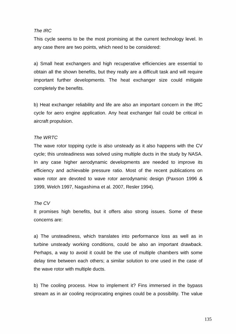
135
The IRC
This cycle seems to be the most promising at the current technology level. In
any case there are two points, which need to be considered:
a) Small heat exchangers and high recuperative efficiencies are essential to
obtain all the shown benefits, but they really are a difficult task and will require
important further developments. The heat exchanger size could mitigate
completely the benefits.
b) Heat exchanger reliability and life are also an important concern in the IRC
cycle for aero engine application. Any heat exchanger fail could be critical in
aircraft propulsion.
The WRTC
The wave rotor topping cycle is also unsteady as it also happens with the CV
cycle; this unsteadiness was solved using multiple ducts in the study by NASA.
In any case higher aerodynamic developments are needed to improve its
efficiency and achievable pressure ratio. Most of the recent publications on
wave rotor are devoted to wave rotor aerodynamic design (Paxson 1996 &
1999, Welch 1997, Nagashima et al. 2007, Resler 1994).
The CV
It promises high benefits, but it offers also strong issues. Some of these
concerns are:
a) The unsteadiness, which translates into performance loss as well as in
turbine unsteady working conditions, could be also an important drawback.
Perhaps, a way to avoid it could be the use of multiple chambers with some
delay time between each others; a similar solution to one used in the case of
the wave rotor with multiple ducts.
b) The cooling process. How to implement it? Fins immersed in the bypass
stream as in air cooling reciprocating engines could be a possibility. The value

136
of kcool=0.08 was taken as a characteristic value from these kind of engines
(Ferguson 2001).
c) The combustion system. The combustion system is complex system to be
study. It will require a further in-depth study. Nalim (1996 & 1999) is devoted to
this crucial topic.
Summarizing, and looking at future development, and attending to the benefits
on SFC and NOx emissions the IRC and the CV are located at a quite similar
level, while for these application the WRTC is clearly at a lower place especially
if we have a look at the NOx emissions. If we consider the benefits on TET and
increase of weight and volume the CV seems to be above the IRC, although it is
complicate to imagine the weight and volume of the CV at this stage. If we
consider the current technological level it is possible to think that the IRC is
located above the CV; the heat exchanger technology for terrestrial application
is well known. Finally the WRTC seems to be a good option for small engines
with low overall pressure to reach a high efficiency with no high penalty on NOx
emission because of a lower maximum pressure and temperature.
5.6 The internal combustion wave rotor (ICWR)
5.6.1 Assumptions
As all models, this engine performance model relies on assumption and
simplifications, which are listed below:
Everything is modeled across engine “bricks” (components) only: on
dimension-related variation is to be taken into account;
Every engine “brick” is tuned with a given set of fixed coefficients;
Only the components aiming at modifying airflows are modeled:
mechanical (bearings, seals, gearboxes…) and electrical components
are not taken into account;

137
Friction and heat transfers along walls are not precisely taken into
account, but are rather included in overall pressure losses;
Airflow modifications are modeled through isentropic relations, but
adjusted with isentropic efficiencies;
Cooling air extraction is modeled at a single location (the chosen
compressor exit) rather than spread over several compressor stages as
in a real engine;
In the same way, the same amount of this cooling air is delivered in a
single location (burner outlet) rather than spread over several turbine
stages;
CVCBIF
OF
CN
WR
BN
AC
INTERNAL COMBUSTION WAVE ROTOR BLOCK DIAGRAM
0
0 12
13 1518
8
2
21 24 454140
31
Bleeds
5
HP
C
3
4
HP
T
LP
T
H
S
0
8
21
24
31
INTERNAL COMBUSTION WAVE ROTOR TOPPING CYCLE
40
45
5
*
*
*3*
*
*41
*
*
2 *
4*
*
*
H
SINTERNAL COMBUSTION WAVE ROTOR BYPASS CYCLE
0
12
13 15
18
*
* *
* *
Figure 73 the INTERNAL COMBUSTION WAVE ROTOR
5.6.2 Result
Figure 74 represents the change of SFC and SPT with the BPR as we can see
beyond a BPR of 18 there is no more improvement of fuel consumption, in fact
it’s quite the opposite, which is because of the increase of the drag generated
by the bigger and bigger nacelle of the engine. Figure 75 shows, as expected,

138
that losses need to be low, this means that the design of the mechanical valves
has to be the most accurate. But from Figure 76 we can see the variation of the
pressure ratio of the cooling compressor with the pressure losses in the wave
rotor – constant volume combustion system. This figure shows how the higher
the losses the smaller needs to be the compressor used to compress the
cooling air that come from the compressor; higher the pressure ratio of this
compressor higher will be the weight of the engine, and this weight increase will
affect the SFC. A trade off analysis needs to be done in order to understand the
magnitude of the acceptable losses in the wave rotor. Figure 77 shows the
variation of SFC and ST against OPR.
After this parametric study a design configuration has been chosen for the
ICWR in order to do a comparison against the VITAL and the advanced
engines. As exemplar for the VITAL engines the GTFLR has been chosen. The
ICWR and the GTF have the following same values (see Table 6, Table 9 and
annex C):
FPR
Fan efficiency
BPR
Booster PR
Booster Efficiency
Turbines efficiencies
Thrust
cooling bleed
OPR
Mass flow
The following table shows the results of the comparison for the four engines
for the SFC and NOx. As we can see in Table 13 the ICWR shows better
results than all the other engines. Once all the technical problems connected
shall be solved this engine seems to be the best solution to the reduction of

139
fuel consumption and emissions, although a noise analysis is needed in
order to understand the noise impact.
% ICR WR CVC ICWR
SFC -2.5 -3.2 -2.5 -4
NOX +0.3 +4 +0.2 -4
Table 13 Comparison between the advanced engines and the GTF
BPR
10.00
10.50
11.00
11.50
12.00
12.50
13.00
13.50
14.00
14.50
15.00
15.50
16.00
16.50
10.00 11.00 12.00 13.00 14.00 15.00 16.00 17.00 18.00 19.00 20.00
BPR
SF
C(m
g/N
se
c)
95.00
100.00
105.00
110.00
115.00
120.00
125.00
130.00
135.00
140.00
145.00
150.00
155.00
SP
T(N
/Kg
/sec)
SFC
SPT
Figure 74: variation of SFC and ST with the BPR
Pressure Losses in the Wave Rotor
0.00
2.00
4.00
6.00
8.00
10.00
12.00
14.00
16.00
18.00
20.00
22.00
24.00
26.00
0.00 0.05 0.10 0.15 0.20 0.25 0.30 0.35 0.40 0.45 0.50 0.55 0.60 0.65 0.70 0.75
Delta P (%)
De
ltaS
FC
(%)
0.00
10.00
20.00
30.00
40.00
50.00
60.00
70.00
80.00
90.00
100.00
110.00
120.00
130.00
140.00
150.00
SP
T(N
/Kg/s
ec)
SFC
SPT
Figure 75 influence of the pressure losses in the ICWR system on the SFC and
ST

140
Pressure Losses in the Wave Rotor
0.00
0.50
1.00
1.50
2.00
2.50
3.00
3.50
4.00
4.50
5.00
0.00 0.05 0.10 0.15 0.20 0.25 0.30 0.35 0.40 0.45 0.50 0.55 0.60 0.65 0.70 0.75 0.80
DP WR (%)
CC
PR
DP WR
Figure 76 variation of the pressure ratio of the cooling compressor with the
pressure losses in the ICWR system
OPR
-10.00
-9.00
-8.00
-7.00
-6.00
-5.00
-4.00
-3.00
-2.00
-1.00
0.00
32.50 43.20 53.14 62.30 71.37 79.71
De
ltaS
FC
(%)
131.00
132.00
133.00
134.00
135.00
136.00
137.00
138.00
139.00
SP
T
SFC
SPT
Figure 77 SFC and ST against OPR.

141
6. Conclusions and Recommendations
6.1 Conclusions
This work describes a method for calculating the direct operating cost of
engines that has been validated using data from public sources and also by
comparison with already existing and well accredited methods. As we have
seen from the results shown, the accuracy of the economic model in DOC
estimation is good (within about 15%), considering the great scattering of data
that can be found for a very large variety of engines, and so can be adapted for
use in the cost analysis of today and future type of engines, such as ultra high
bypass ratio turbofans, with little modifications.
A method for calculating the direct operating cost of aero engines has been
applied to three different types of configurations of advanced type of turbofans
used for long and short range applications: the direct drive, the geared and the
counter rotating turbofans. The model shows that, if any type of future engines
would be considered economically advantageous, current technology has to be
improved and costs of production have to decrease by around 35%, because
they are the main driving factors for the cost of operation of engines.
Using the risk module a sensitivity analysis has been done in order to
understand the impact of the different economic parameters on the operational
costs. Considering today legislation and common core technology for the
different VITAL engines the bigger drivers are fuel burn and carbon tax, instead
NOx and noise have quite low impact. But we need to keep in mind that for sure
the legislation will soon change then a study has been done in order to
understand which would be the main drivers in the design of future engines.
The analysis has shown that noise will be most probably the main constraint to
be taken into consideration.

142
Weibull distributions have been used into the life analysis of different parts of
the engine in order to estimate the cost of maintenance, the direct operating
costs (DOC) and net present cost (NPC) of future type turbofan engines.
The Weibull risk assessment has been applied to four different engines of
different thrust in order to show the applicability of the method to all type of
engines.
Five Weibull distributions have been used for five important sources of
interruption of the working life of the engine: Combustor, Life Limited Parts
(LLP), High Pressure Compressor (HPC), General breakdowns and High
Pressure Turbine (HPT).
As it was shown in the results, the components that are more likely to
breakdown are the HPT and the HPC, keeping in mind that general causes of
breakdown are very difficult to predict.
The distributions used in the work are the same for all the engines, so the
results are quite similar for all of them. But the use of more specified
distributions will led to more accurate predictions. In this thesis it has been
proved that the Weibull method can be used with great success in forecasting
the possible breakdown causes of gas turbines. The analysis of the life of the
different components done with the Weibull is one-dimensional and quite
general, but it still is useful to help the designer in order to do a risk assessment
of the engine.
Optimisation was done on the VITAL engines in order to improve them. It was
done using two numerical gradient based techniques. Firstly the Sequential
Quadratic Programming – NLPQL and secondly the Mixed Integer Optimization
– MOST; the objectives of the optimisation were two: minimum fuel burn and
minimum direct operating costs. Because the engines were already designed
for minimum fuel burn, the optimization for minimum fuel burn showed only a
slight improvement; instead the results for minimum DOC showed that the
engines can be greatly got better, between 2 and 6 percent.

143
As can also be seen by the input files the new engines cannot achieve the
decrease in noise and gaseous emissions required by ACARE. Then it has
been presented a parametric study of three possible configurations that could
accomplish the task. The three engines are:
Intercooled recuperated
Wave rotor topped cycle
Constant volume combustion
These three cycles have been applied to a characteristic next generation long
range aero engine looking for a possible future evolution and searching for
benefits on specific thrust fuel consumption, emissions and economics. The
parametric study has been applied to TOC (Top of Climb) and cruise conditions,
and considering two possible designs:
a) Design for constant specific thrust and
b) Design for constant TET considering the current technology level limit;
Both values correspond to the baseline engine at respective flight conditions.
The study leads to the following conclusions:
a) A significant decrease of specific fuel consumption can be obtained for the
new three cycles. These benefits can reach values close to 10%, depending on
the cycle.
b) The benefits on SFC can also be translated into benefits on NOx emissions.
An exception is the wave rotor topping cycle which will increase NOx emissions
due to a high increase of maximum cycle pressure and temperature.

144
c) The case of design condition for constant specific thrust also leads to
significant lower engine TETs, which will increase the engine life. These
benefits are extremely high in the case of CV cycle.
d) The three cycles will need important technological developments, especially
the wave rotor topping cycle and the CV cycle. The intercooled recuperated
cycle seems to be the most achievable at the current technological level; we
have to keep in mind it comes from typical applications in sea and terrestrial
power generation.
e) About the impact of weight in the ICR it can be said:
The increase of weight and drag can nullify all benefits on SFC for
ηR=0.7
Instead for values of ηR=0.8 or higher, which could represent an
achievable value with the appropriate technologic development,
important benefits can be got even for important increases of weight and
size; a 100% increase of drag translates into an increase of engine
diameter of 41%, assuming that the drag goes as the square of the
engine diameter.
The maximum benefits on total fuel consumption correspond to ηR=0.9,
but it represents a difficult value to be achieved even in terrestrial
application where the weight and size of the heat exchangers do not
represent a critical constraint.
Small heat exchangers and high recuperative efficiencies are essential to
obtain all the shown benefits, but they really are a difficult task and will
require important further developments. The heat exchanger size could
mitigate completely the benefits.
Heat exchanger reliability and life are also an important concern in the
IRC cycle for aero engine application. Any heat exchanger fail could be
critical in aircraft propulsion.
Considering the existing experience on later recuperated engines the
author believes that this engine can achieve the ACARE goals of 2020.

145
6.2 Recommendations for future works
Being a study about future engines, done using the innovative approach of
coupling all the main aspects of first design engines, many things can be done
in the future.
First of all the lifing code can be improved in several ways. Some suggestions
are here mentioned:
having talked about and described carefully how temperature really
affects the results, playing a primary role in the failure mechanism, a
useful and recommended improvement would be the implementation of a
more sophisticate cooling mechanism;
Another issue to cope with is the changing in the material mechanical
properties with the temperature: this phenomenon is even more evident
at elevated temperature, as it is in the ‘hot section’ of the engine, causing
the material to behave totally different from what it would have done at
room temperature.
The lifing analysis can be improved including all the possible type of
stress that affect the HPT blades and disk
And also introducing life analysis of other engine components, like
compressor or, for the future configurations, the counter rotating fan, the
gear, the wave rotor, the CVC and the heat exchangers.
The Weibull distributions can be improved using real data for each
component of each engine.
Also a risk analysis should be conducted in order to see the impact of different
type of legislations on the operating costs.
Detailed performance analysis of the design point and off design point operation
of engines fitted with ICWR’s. Accounting for the various losses that occur in

146
ICWR’s would lead to better design procedures. Analysis of the noise generated
and the various noise abatement techniques that can be used to reduce the
aforementioned noise levels need to be investigated.
The types of materials required along with various failure modes and a
feasibility study would need to be conducted. This would help engineers decide
as to whether ICWR’s are reliable and feasible.
Numerically simulating a complete ICWR with combustion along with various
losses would need to be conducted. This would need to thorough understanding
of the various flow characteristic that are present within a working ICWR.
More work can be done also under the optimisation point of view. Different
optimisation techniques could be used and a comparison between the results
can be done. An optimisation of the intercooled recuperated, wave rotor and
constant volume combustion engines should be done in order to further improve
them. A multi trade – off analysis should be done in order to see which kind of
design is preferable: one with minimum fuel burn or minimum direct operating
costs, and also to see if it is possible to find a configuration that can achieve
both results.
6.3 Author’s contributions to knowledge
The contribution to knowledge that the author thinks can give to the scientific
community with his research comes in two forms:
1. The creation of a tool that can optimise the one dimensional design of
aero engines in a new way. Thermo Economic and Risk Analysis (TERA)
will be in fact a new way to optimise all the characteristics that are
needed to be taking into account in the design of an engine, such as
engine and aircraft performance, weight, noise, emissions and the
operating costs. In TERA my scope is the creation of an economic and a
performance models that can study the operating costs and the

147
performance of aero engines. The economic model is divided into three
modules: a lifing module, a risk module and an economic module.
2. The performance analysis of new cycle engines that can achieve the
goals of ACARE to decrease the emissions of CO, NOX and CO2 by
50%. With the help of TERA the design of this new type of engine will be
much facilitated.

148
References
1. Aircraft Commerce: Issues No. 5, 23, 30, 38, 39, 44
2. Barrett, M. J., Expectations of Closed-Brayton-Cycle Heat Exchangers in
Nuclear Space Power Systems, J. of Propulsion and Power, 21 (1),
January-February 2005, 152-157.
3. Baudier, D. and Piquet, F., 2004. Snecma, a VITAL player. Snecma
Magazine, November, p.28.
4. Beck, D. S., Optimization of Regenerated Gas Turbines, J. of
Engineering for Gas Turbine and Power, 118, July 1996, 654-660.
5. Bhargava, R., Bianchi, M., Peretto, A., Spina, P. R., A Feasibility Study of
Existing Gas Turbines for Recuperated, Intercooler, an Reheat Cycle, J.
of Engineering for Gas Turbine and Power, 126, July 2004, 531-544.
6. Cai, R., A new Analysis of Recuperative Gas Turbine Cycles, Proc. Instn.
Mech Engnrs Vol 212 Part A, 1998, 289-296.
7. Cambier, J. L., Tegner, J. K., Strategies for Pulsed Detonation Engine
Performance Optimization, J. of Propulsion and Power, 14 (4), July-
August 1998, 489-498.
8. Corchero, G., Montañes, J. L., An Approach to the Use of Hydrogen for
Commercial Aircraft Engines, Proc. IMechE Vol. 219 Part G: J.
Aerospace Engineering, 2005, 35-43.
9. Dellenback, P. A., Improved Gas Turbine Efficiency through Alternative
Regenerator Configuration, J. of Engineering for Gas Turbine and Power,
124, July 2002, 441-446.
10.Environmentally Friendly Aero Engine (VITAL). Sixth Framework
Program of the European Communities, contract AIP4-CT-2004-012271,
2004.
11.ETBX Strain-Life Fatigue Analysis [online]. EngineersToolbox.
http://www.engrasp.com/doc/etb/mod/fm1/strainlife/strainlife_help.html
12.Ferguson, C., R., Kirkpatrick, Internal Combustion Engines, Applied
Thermosciences, John Willey & Son, Inc, New York, 2001, chap. 8.
13.Flight international: Issues no. 5022-5050

149
14.Haslam “Fracture and fatigue course notes” Cranfield University.
15.Haslam “Mechanical design of turbo machinery course notes” Cranfield
University.
16.Heiser, W. H., Pratt, D. T., Thermodynamic Cycle Analysis of Pulse
Detonation Engines, J. of Propulsion and Power, 18 (1), January-
February 2002, 68-76.
17.Henry T. Won and Mark Waters, Constant Volume Combustor
implementation on a 50 passenger Commercial Regional Transport
Mission Simulation, 39th AIAA/ASME/SAE/ASEE Joint Propulsion
Conference and Exhibit 20-23 July 2003, Huntsville, Alabama.
18.Hill, P. G., Peterson, C. B., Mechanics and Thermodynamics of
Propulsion, Addison-Wesley, London, 1965.
19.Howse, M., Rolls-Royce and Gas Turbine,16th ISABE International
Symposium on Air Breathing Engines, Cleveland, Ohio, USA, September
2003, AIAA paper 2003-1002.
20.http://www.boeing.com/commercial/noise/index.html
21.Jenkinson, Lloyd R. Paul Simpkin, Darren Rhodes: “Civil jet aircraft
Design” London: Arnold, 1999.
22.Johnsen, A., Bullock, R. O., Aerodynamic Design of Axial-Flow
Compressors, NASA SP-36, 1965, chap. II.
23.Kays, W. M., London, A. L. Compact Heat Exchangers, Krieger
Publishing Company, Malabar, Florida, 1984.
24.Kentfield, J. A. C., Fundamentals of Idealized Airbreathing Pulse-
Detonation Engines, J. of Propulsion and Power, 18 (1), January-
February 2002, 77-83.
25.Kentfield, J. A. C., Regenerative Turbofans; A Comparison with Non
regerative Units, J. of Aircraft, 12 (3), March 1975, 174-181.
26.Klug, H. G., Reinhard, F., CRYOPLANE: Hydrogen Fuelled Aircraft –
Status and Challenges, Air&Space Europe, 2001, 3 (3), 252-254.
27.Lefebvre, A. H., Fuel Effects on Gas Turbine Combustion-Liner
Temperature, Pattern Factor, and Pollutants Emissions, J. of Aircraft,
21(11), November 1984, 887-898.
28.Lefebvre, A. H., Gas Turbine Combustion, Taylor & Francis,

150
Philadelphia, London, 1998.
29.Lenoble G. Performance Analysis of a Wave Rotor Topping Unit with
Constant Volume Combustion, Cranfield University MSc Thesis, 2008
30.Lewis, G. D., A new Understanding of NOx formation, 10th ISABE
International Symposium on Air Breathing Engines, Nottingham,
England, 1991, paper ISABE 91-7064.
31.Liquid Hydrogen Fuelled Aircraft – System Analysis (CRYOPLANE), Part
B Proposal GRD1-1999-10014, Fifth Framework Program of the
European Communities, contract G4RD-CT-2000-00192, June 1999.
32.Liu, F., Sirignano, W. A., Turbojet and Turbofan Engine Performance
Increases through Turbine Burners, J. of Propulsion and Power, 17 (3),
May-June 2001, 695-705.
33.Management for technology course notes Cranfield University.
34.Manson, S. S., 1965. Fatigue: A Complex Subject—Some Simple
Approximations. Experimental Mechanics. Journal Society For
Experimental Stress Analysis, 5 (7),193–226.
35.Martinez-Frias, J., Aceves, S. M., Brandt, H., Thermodynamic Analysis of
Zero- Atmospheric Emissions Power Plant, J. of Engineering for Gas
Turbine and Power, 126, January 2004, 2-8.
36.Mattingly, J. D., Heiser, W. H., Prat, D. T., Aircraft Engine Design, AIAA
Education Series, American Institute of Aeronautics and Astronautics,
Inc, Reston, Virginia, 2002.
37.Meggiolaro, J.T.P. Castro: “Statistical evaluation of strain-life fatigue
Crack initiation predictions”, 2004, International Journal of Forecasting
38.Missirlis, D., et al, Experimental and Numerical Investigation of Flow
Field through a Heat Exchanger for Aero-engine Applications, Int. J. of
Heat and Fluid Flow, 26, 2005, 440-458.
39.Nagashima, T., Okamoto, K., Simple Numerical Modelling for
Gasdynamic Design of Wave Rotors, J. of Propulsion and Power, 23 (1),
January-February 2007, 99-107.
40.Nalim, M. R., Assessment of Combustion Modes for Internal Combustion
Wave Rotors, J. of Engineering for Gas Turbine and Power, April 1999,
121, 265-271

151
41.Nalim, M. R., Paxson, D. E., A Numerical Investigation of Premixed
Combustion in Wave Rotors, NASA TM-107242, 41st Gas Turbine and
Aero engine Congress, Birmingham, UK, June 10.13, 1996, paper
ASME-96-GT-116.
42.Nalim, M. R., Thermodynamic Limits of Work and Pressure Gain in
Combustion and Evaporation Processes, J. of Propulsion and Power, 18
(6), November-December 2002, 1176-1182.
43.Nalim, R. M., Resler Jr, E. L., Wave Cycle Design for Wave Rotor Gas
Turbine Engines with Low NOx Emissions, J. of Engineering for Gas
Turbine and Power, July 1996,118, 474-480.
44.New Aero Engine Concept (NEWAC). Sixth Framework Programme of
the European Communities, 2006.
45.Paxson, D. E., Lindau, W. J., Numerical Assessment of Four-Port
Through-Flow wave Rotor Cycles with Passage Height Variation, NAS
TM-107490, 33rd Joint Propulsion Conference and Exhibit, Seattle,
Washington, July 1997.
46.Paxson, D. E., Nalim, M. R., Modified Through-Flow Wave-Rotor Cycle
with Combustor- Bypass Ducts, J. of Propulsion and Power, 151 (3),
May-June 1999, 462-467.
47.Paxson, D. E., Numerical Simulation of Dynamic Wave Rotor
Performance, J. of Propulsion and Power, 12 (5), September-October
1996, 949-957.
48.Pilidis “Gas turbine performance course notes” Cranfield University.
49.Ramsden “Turbo machinery course notes” Cranfield University.
50.Resler Jr, E. L., Moscari, J. C., Nalim, M. R., Analytic Design Methods for
Wave Rotor Cycles, J. of Propulsion and Power, 10 (5), Sept.-Oct. 1994,
683-689.
51.Roskam, Jan: “Airplane design. Part VIII, Airplane cost estimation:
design, Development, manufacturing and operating” Ottawa, Kansas:
Roskam Aviation and Engineering Corporation, 1990.
52.Rubini, P., 2006. Turbine Blade Cooling. MSc course notes. Cranfield
University.
53.Saravanamamuttoo, H. I. H., Gas Turbine Theory, Pearson, England,

152
2001.
54.Sawyer, W. J., Sawyer’s Gas Turbine Engineering Handbook, Gas
Turbine Publications, Inc, Stamford, Connecticut, USA, 1972.
55.Sehra, A. K., Shin, J., Revolutionary Propulsion Systems for 21st
Century Aviation, NASA TM-2003-212615, International Gas Turbine
Congress 2003, Tokyo, Japan, November 2-7, 2003, paper IGTC03-
ABS-066b.
56.Sirignano, W. A., Liu, F., Performance Increases for Gas-Turbine
Engines through Combustion inside the Turbine, J. of Propulsion and
Power,15(1), January-February 1999, 111-118.
57.Smith, C. P., The environmental Challenge – Bringing Technology to
Market, 17th ISABE International Symposium on Air Breathing Engines,
Munich, Germany, September 2005, paper ISABE-2005-1008.
58.Smith, C.F., Snyder, P.H., Emmerson, C.W. Nalim, M.R., Impact of the
CVC on a Supersonic Turbofan Engine, 38th AIAA/ASME/SAE/ASEE
Joint Propulsion Conference & Exhibit 7-10 July 2002, Indianapolis,
Indiana.
59.Sourmail, T., no date. Coatings for Turbine Blades [online]. University of
Cambridge. Available from: http://www.msm.cam.ac.uk/phase-
trans/2003/Superalloys/coatings/index.html [Accessed July 2006].
60.Steffen, K., Walter, R., Driving the Technological Edge in Airbreathing
Propulsion, 16th ISABE International Symposium on Air Breathing
Engines, Cleveland, Ohio, USA, September 2003, AIAA paper 2003-
1002.
61.TERA high level specification document
62.Thomas N. R. Preliminary Design and Analysis of an Internal
Combustion Wave Rotor, Cranfield University MSc Thesis, 2008
63.Vigna Suria O., “A Flexible Lifing Model for Gas Turbines: Creep and
Low Cycle Fatigue Approach”, Cranfield University, master thesis, 2006.
64.Walsh, P. P., Fletcher, P., Gas Turbine Performance, Blackwell Science,
Ltd, London, 1998.
65.Weekly Petroleum Status Report/Energy Information Administration
January 2005, February 2006

153
66.Welch, G. E., Jones, S. M., Paxson, D. E., Wave-Rotor-Enhancement
Gas Turbine Engines, J. of Engineering for Gas Turbine and Power, 119,
April 1997, 469-477.
67.Welch, G. E., Macroscopic Balance Model for Wave Rotor, J. of
Propulsion and Power, 13 (4), July-August 1997, 508-516.
68.Welch, G. E., Paxson, D. E., Wave-Rotor-Enhanced Gas Turbine Engine
Demonstrator, NASA TM-1999-209459, Gas Turbine Operation and
Technology for Land, Sea and Air Propulsion and Power System
Symposium, Ottawa, Canada, October 18-21, 1999.
69.Welch, G. E., Wave Engine Topping Cycle Assessment, NASA TM-
107371, 35th Aerospace Science Meeting and Exhibit, paper AIAA-97-
0707, Reno, Nevada, January 1997.
70.Wilson, J., an Experiment on Losses in a Three-Port Wave Rotor, NAS
CR-19508, 1997.
71.Wilson, J., Paxson, D. E., Jet Engine Performance Enhancement through
Use of a Wave-Rotor Topping Cycle, NASA TM-4486, 1993.
72.Wilson, J., Paxson, D. E., Wave Rotor Optimization for Gas Turbine
Engine Topping Cycles, J. of Propulsion and Power, 12 (4), July-August
1996,778-785.
73.Wulff, A., Hourmouziadis,J., An Universal Combustor Model for the
Predictions of Pollutant Emissions, 15th ISABE International Symposium
on Air Breathing Engines, paper ISABE 99-7162, 1999.
74.www.icaodata.com
75.www.weibull.com
76.Yakinthos, et al, Optimization of the Design of Recuperative Heat
Exchangers in the Exhaust Nozzle of an Aero-Engine, Appli Math Mod,
2006, doi: 10.1016/J.a.p.m.2006.10.008.

154
Appendix A – Economic Model Input Files
! EcoModuleInput.dat
! Input file for the Economic Program
! This file requires both user defined variables for a given power plant/aircraft.
It has been separated into SR and LR
! Some of the parameters are regularly updated parameters during the
optimisation done and explained in paragraph 5.4. In red are shown the
parameters obtained by other modules and passed to the economic through
iSight and then changed during the optimisation.BASELR : Engine configurationRene80 :blade MATERIALRene95 :disk material23000 :TBO (Hr) (This value is used when the Lifing cannot do the calculations)316.296000 :Take-off Thrust,AcToFN (kN)7.877100 :Block Time,AcBlockTime (Hr)5879.780000 :Plant Cost,PCost (k€)82533.090000 :WEIGHT OF FUEL USED,AcBlockFuel (Kg)817 :Fuel density (Kg/cubic meter)27000 :Threshold for the Carbon Tax (Kg)5 :Carbon Tax Charge (€/kg)12048.410000 :BLOCK DISTANCE (RBL),AcBlockRng (Km)0.005 :INSURANCE PERCENTAGE (ISP)103.210000 :EPNLarr (dB)99. :EPNLdep (dB)24419.485400 :NOX, MNoxLto (g)0.8222 :exchange rate $ -> € (ROC)22.065300 :D/Foo CO, DFCO (-)30 :EXPECTED OPERATING ENGINE LIFE (NYEARS)1 :NUMBER OF SCENARIOS5. :NOX TAX CHARGE (€/kg)172. :FUEL PRICE (FP)0.1 :INTEREST PERCENTAGE (IP)0.02 :INFLATION (INF)89.9 :NOISE TAX Limit (dB)100 :Unit of cost of Decibel (€/dB)1.5 :NOX FACTOR (B)10. :DOWNTIME70. :MAINTENANCE labour Rate Per Man Hour (RLENG) (€/Hr)1 :Selector of IP (1:constant for every scenario; 2:change every scenario)2 :SELECTOR OF FUEL PRICE2 :SELECTOR OF NOX FACTOR2 :SELECTOR OF DOWNTIME2 :SELECTOR OF INFLATION2 :SELECTOR OF MAINTENANCE labour RATE PER MAN HOUR2 :Selector of Threshold for the Carbon Tax (Kg)2 :Selector of NOISE TAX Limit2 :selector of weibull60. :Minimum Value of FUEL Price (c$/US gallon)200. :Maximum Value OF FUEL PRICE0.05 :Minimum Value of INTEREST PERCENTAGE0.2 :Maximum Value OF INTEREST PERCENTAGE0.01 :Minimum Value of INFLATION0.03 :Maximum Value OF INFLATION1.1 :Minimum Value of NOX FACTOR2. :Maximum Value OF NOX FACTOR1. :Minimum Value of DOWNTIME (days)90. :Maximum Value OF DOWNTIME50. :MINIMUN Value of Maintenance labour Rate Per Man Hour70. :MAXIMUM Value of Maintenance labour Rate Per Man Hour21000. :minimum Value of Threshold for the Carbon Tax (Kg)27000. :Maximum Value of Threshold for the Carbon Tax (Kg)89. :MINIMUN VALUE OF NOISE TAX Limit94. :Maximum Value of NOISE TAX Limit
Below are shown the typical input file for the lifing module, first for creep with
analysis of the stresses for the blades and the disk of the high pressure

155
turbine that is the element in a gas turbine that most limit the life of the engine
and then the input data necessary for the analysis of fatigue also applied to
the blades of the high pressure turbine:
! blade_stress_input.dat
1 :number of section the blade has been split into0.347156 :inner radius0.392258 :outer radius0.000273 :inner cross area0.000191 :outer cross area
!disc_input.dat1. :disc type selector (1 = constant thickness disc; 2 = varying thickness disc)1. :rim stress selector (1 = Rim stress to be calculated using the blade stress subroutine; 2 = Rim stressto be calculated knowing number of blades, balde mass and radius of the centre of gravity; 3 = rim stress known)0.694311 :rim diameter0.171014 :bore diameter0.030068 :disc constant thickness68.000000 :number of blades4. :number of rings into which the disc is discretized0.09820 :inner radius (m) of the first ring0.03710 :thickness (m) of the first ring0.12840 :inner radius (m) of the second ring0.02000 :thickness (m) of the second ring0.15590 :inner radius (m) of the third ring0.00930 :thickness (m) of the third ring0.27670 :inner radius (m) of the fourth ring0.01836 :thickness (m) of the fourth ring0.32150 :radius (m) of the boundary0.01836 :thickness (m) of the boundary
! indat_creep.dat
3. :number of segments into which the flight envelope has been split221.098000 :HPT rpm @ design point1. :blade stress selector (1 = stress unknown, a stress subroutine will calculate it; 2 = stress known)1. :disk stress selector (1 = stress unknown, a stress subroutine will calculate it; 2 = stress known)1. :cooling selector (1 = blade cooled; 2 = no cooling)0.5 :cooling effectiveness150. :Delta of Temperature due to Termal Barrier Coating on the blade1. :blade Larson-Miller selector (1 = insert values to be interpolated; 2 = LMP known for each segment)1. :disk Larson-Miller selector (1 = insert values to be interpolated; 2 = LMP known for each segment)0.980000 :relative rpm during the climb0.914550 :relative rpm acting during the cruise0.807730 :relative rpm acting during the descent923.660000 :cooling temperature during climb830.630000 :cooling temperature during cruise710.960000 :cooling temperature during descent1888.000000 :temperature in K acting during the climb1640.000000 :temperature in K acting during the cruise1278.000000 :temperature in K acting during the descent16.001550 :time in hours spent during the climb339.655600 :time in hours spent during the cruise21.267750 :time in hours spent during the descent
If the stresses are known for each segment for the blade and/or the disk put
below all the stresses in MPa first for the blade and/or then for the disk, the
same applies if the Larson-Miller parameter for each segment of flight is
known. First put all the stresses and then all the LMPs for the blade and then
do the same for the disk
! Indat_fatigue.dat
288. :Ambient temperature in Kelvin2011.000000 :Component maximum operating temperature in Kelvin1. :cooling selector (1 = blade cooled; 2 = no cooling)997.240000 :cooling flow temperature0.5 :cooling effectiveness150 :delta temperature for coating

156
! INPUTweibull.txt
5 :NUMBER OF DISTRIBUTIONS0.0 :ETA HPT0.12 :ETA COMBUSTOR0.20 :ETA LLP0.22 :ETA HPC0.45 :ETA GENERAL6 :BETA HPT4.5 :BETA COMBUSTOR4 :BETA LLP3 :BETA HPC1.5 :BETA GENERAL
! material_database.txt
DSCM247 :Material specifier20.0 :Larson Miller (LM) constant6 :Number of data in LM curve
51.84 20.5 :LM curve (stress in (Ksi)). LM parameters in decreasing order.50.1 30.0 :48.0 47.0 :46.9 55.0 :45.9 65.0 :44.9 74.0 :
8910.0 :Material density (kg/m^3)1 :No data in yield stress (ys) curve. Temp. in K. ys in MPa
300.00 890.0 :215000.0 :Elastic modulus of the material in MPa0.15 :Fatigue ductility coefficient in mm1573.0 :Fatigue strength coefficient in MPa-0.08 :Fatigue strength exponent-0.59 :Fatigue ductility exponent11.0E-6 :Linear coefficient of thermal expansion in mm/°C0.29 :Poisson's ratio1 :LM equation selector (1 = equation in Imperial Units, 2 = equation in SI)!----------------------------------Nimo118 :Material specifier20.0 :Larson Miller (LM) constant6 :Number of data in LM curve
28.7 80.0 :LM curve (stress in (MPa)). LM parameters in decreasing order28.4 90.0 :28.0 100.0 :27.0 150.0 :26.4 200.0 :25.7 250.0 :
8190.0 :Material density (kg/m^3)1 :No data in yield stress (ys) curve. Temp. in K. ys in MPa
300.00 800.0 :222000.0 :Elastic modulus of the material in MPa0.40 :Fatigue ductility coefficient in mm1820.0 :Fatigue strength coefficient in MPa-0.08 :Fatigue strength exponent-0.59 :Fatigue ductility exponent12.7E-6 :Linear coefficient of thermal expansion in mm/°C0.32 :Poisson's ratio2 :LM equation selector (1 = equation in Imperial Units, 2 = equation in SI)!----------------------------------MarM247 :Material specifier20.0 :Larson Miller (LM) constant6 :Number of data in LM curve
53.1 11.5 :LM curve (stress in (Ksi)). LM parameters in decreasing order.49.0 30.0 :46.56 50.0 :44.0 66.0 :42.5 84.0 :41.0 100.0 :
8540.0 :Material density (kg/m^3)1 :No data in yield stress (ys) curve. Temp. in K. ys in MPa
300.00 827.0 :221000.0 :Elastic modulus of the material in MPa0.177 :Fatigue ductility coefficient in mm1351.0 :Fatigue strength coefficient in MPa-0.12 :Fatigue strength exponent-0.6 :Fatigue ductility exponent11.0E-6 :Linear coefficient of thermal expansion in mm/°C0.29 :Poisson's ratio1 :LM equation selector (1 = equation in Imperial Units, 2 = equation in SI)!----------------------------------IMI_829 :Material specifier20.0 :Larson Miller (LM) constant0 :Number of data in LM curve4540.0 :Material density (kg/m^3)1 :No data in yield stress (ys) curve. Temp. in K. ys in MPa
300.00 996.7 :109000.0 :Elastic modulus of the material in MPa0.5 :Fatigue ductility coefficient in mm1913.3 :Fatigue strength coefficient in MPa-0.10 :Fatigue strength exponent-0.69 :Fatigue ductility exponent9.5E-6 :Linear coefficient of thermal expansion in mm/°C
0.33 :Poisson's ratio1 :LM equation selector (1 = equation in Imperial Units, 2 = equation in SI)!----------------------------------Inco718 :Material specifier

157
25.0 :Larson Miller (LM) constant6 :Number of data in LM curve
36 50.0 :LM curve (stress in (MPa)). LM parameters in decreasing order.34 100.0 :32 172.0 :30 303.0 :28 400.0 :26 500.0 :
8220.96 :Material density (kg/m^3)1 :No data in yield stress (ys) curve. Temp. in K. ys in MPa
300.00 1122.64 :205000.0 :Elastic modulus of the material in MPa0.35 :Fatigue ductility coefficient in mm1736.0 :Fatigue strength coefficient in MPa-0.08 :Fatigue strength exponent-0.59 :Fatigue ductility exponent11.5E-6 :Linear coefficient of thermal expansion in mm/°C0.29 :Poisson's ratio2 :LM equation selector (1 = equation in Imperial Units, 2 = equation in SI)!----------------------------------Rene95 :Material specifier20.0 :Larson Miller (LM) constant6 :Number of data in LM curve
30 50.0 :LM curve (stress in (MPa)). LM parameters in decreasing order28.4 100.0 :26.3 300.0 :25 500.0 :23 620.0 :21 850.0 :
8248.64 :Material density (kg/m^3)1 :No data in yield stress (ys) curve. Temp. in K. ys in MPa
300.00 1274.99 :218000.0 :Elastic modulus of the material in MPa0.15 :Fatigue ductility coefficient in mm1785.0 :Fatigue strength coefficient in MPa-0.08 :Fatigue strength exponent-0.59 :Fatigue ductility exponent11.3E-6 :Linear coefficient of thermal expansion in mm/°C0.3 :Poisson's ratio2 :LM equation selector (1 = equation in Imperial Units, 2 = equation in SI)!----------------------------------Udimet720 :Material specifier20.0 :Larson Miller (LM) constant6 :Number of data in LM curve
29.9 50.0 :LM curve (stress in (MPa)). LM parameters in decreasing order.28.8 100.0 :27.7 200.0 :26 300.0 :25 400.0 :24 700.0 :
8080.0 :Material density (kg/m^3)1 :No data in yield stress (ys) curve. Temp. in K. ys in MPa300 1150.0 :
220000.0 :Elastic modulus of the material in MPa0.15 :Fatigue ductility coefficient in mm1561.0 :Fatigue strength coefficient in MPa-0.08 :Fatigue strength exponent-0.59 :Fatigue ductility exponent12E-6 :Linear coefficient of thermal expansion in mm/°C0.3 :Poisson's ratio2 :LM equation selector (1 = equation in Imperial Units, 2 = equation in SI)!----------------------------------Waspalloy :Material specifier20.0 :Larson Miller (LM) constant6 :Number of data in LM curve
30.3 50.0 :LM curve (stress in (MPa)). LM parameters in decreasing order.28.2 100.0 :27.1 200.0 :25.4 327.5 :23.7 517.0 :21.5 700.0 :
8190.0 :Material density (kg/m^3)1 :No data in yield stress (ys) curve. Temp. in K. ys in MPa
294.26 792.86 :211000.0 :Elastic modulus of the material in MPa0.15 :Fatigue ductility coefficient in mm1118.0 :Fatigue strength coefficient in MPa-0.08 :Fatigue strength exponent-0.59 :Fatigue ductility exponent12.2E-6 :Linear coefficient of thermal expansion in mm/°C0.3 :Poisson's ratio2 :LM equation selector (1 = equation in Imperial Units, 2 = equation in SI)!----------------------------------CMSX4 :Material specifier20.0 :Larson Miller (LM) constant6 :Number of data in LM curve
30.9 120.0 :LM curve (stress in (MPa)). LM parameters in decreasing order30.2 137.2 :29.4 160.0 :28.8 200.0 :27.5 300.0 :26.9 392.0 :
8700.0 :Material density (kg/m^3)8 :No data in yield stress (ys) curve. Temp. in K. ys in MPa297.15 942.0 :
250000.0 :Elastic modulus of the material in MPa0.15 :Fatigue ductility coefficient in mm1413.0 :Fatigue strength coefficient in MPa-0.08 :Fatigue strength exponent-0.59 :Fatigue ductility exponent11E-6 :Linear coefficient of thermal expansion in mm/°C0.3 :Poisson's ratio

158
2 :LM equation selector (1 = equation in Imperial Units, 2 = equation in SI)!----------------------------------ReneN5 :Material specifier20.0 :Larson Miller (LM) constant6 :Number of data in LM curve
29.4 141.0 :LM curve (stress in (MPa)). LM parameters in decreasing order.28 237.0 :27 324.0 :26 427.0 :25 549.0 :24 676.0 :
8630.0 :Material density (kg/m^3)1 :No data in yield stress (ys) curve. Temp. in K. ys in MPa
300.00 1260 :219000.0 :Elastic modulus of the material in MPa0.17 :Fatigue ductility coefficient in mm1770.0 :Fatigue strength coefficient in MPa-0.1 :Fatigue strength exponent-0.61 :Fatigue ductility exponent11.8E-6 :Linear coefficient of thermal expansion in mm/°C0.3 :Poisson's ratio2 :LM equation selector (1 = equation in Imperial Units, 2 = equation in SI)!----------------------------------Rene80 :Material specifier20.0 :Larson Miller (LM) constant6 :Number of data in LM curve
31.4 50 :LM curve (stress in (MPa)). LM parameters in decreasing order30.2 100 :29 150 :
28.04 200 :27.24 250 :26.52 300 :
8160.0 :Material density (kg/m^3)1 :No data in yield stress (ys) curve. Temp. in K. ys in MPa
300.00 1274.99 :217000.0 :Elastic modulus of the material in MPa0.16 :Fatigue ductility coefficient in mm1780 :Fatigue strength coefficient in MPa-0.09 :Fatigue strength exponent-0.60 :Fatigue ductility exponent11.5E-6 :Linear coefficient of thermal expansion in mm/°C0.3 :Poisson's ratio2 :LM equation selector (1 = equation in Imperial Units, 2 = equation in SI)

159
Appendix B – Economic Model Output Files
Amongst the outputs the economic model would give are:
Direct operating cost, DOC (k€)
Engine maintenance cost (k€)
Net present cost, NPC.
The NPC would be obtained over a time frame defined by the user to depict
the engine operating life.
A typical output from the economic model is show below:-
! EcoModuleOutput.dat
*********************************************************************OUTPUT, Courtesy of:09-APR-0813:08:45Configuration: BASELR*********************************************************************ANNUAL UTILIZATION /YEAR (Hr) = 4400.000COST OF LANDING FEES /FLIGHT (k€) = 1.380000COST OF NAVIGATIONAL FEES /FLIGHT (k€) = 5.168192COST OF GROUND HANDLING CHARGES /FLIGHT (k€) = 3.30000XXXXXXXXXXXXX SCENARIO STUDIES XXXXXXXXXXXXXXXXXXXXSCENARIO =1
XXXXXXXXXXXXXXX SUMMARY OF RESULTS FOR YEAR 1 XXXXXXXXLabour/Eng/BlockHr (k€/Hr) = 0.6296688NOx Tax (k€/Flight) = 0.1868091CarbonTax (k€/Flight) = 283.2188Mtrls/Eng/BlockHr (k€/Hr) = 0.2746555DoCMtce/Eng/Hr (k€/Hr) = 0.9043242DoC/Eng/Yr (k€/Year) = 123957.1CFUEL/Yr (k€/Year) = 14350.40NoiseTax (k€/Flight) = 9.143278AirportTax (k€/Year) = 103854.9XXXXXXXXXXXXXXXXXXXXXXXXXXXXXXXXXXXXXXXXXXXXXXX
WEIBULL TIME BETWEEN OVERHAUL = 995.0844ENGINE NPC FOR 30 YEARS (k€) = 17347
Below it is given a typical output used to generate the cumulative curve from
the economic model with the risk model changing all the variables apart from
the IP for 10000 scenarios.
!NPCoutput.dat
ENGINE NPCMAXIMUM NPC (k€) = 7924MINIMUM NPC (k€) = 7666LENGHT OF INTERVALS = 23Medium value of interval (k€) frequency (%) cumulative frequency (%)
7677 3 37700 1 47723 8 127746 18 30

160
7769 28 587792 8 667815 19 857838 6 917861 0 917884 6 977907 1 98
!blade_stress_output.dat
sec_cf_load = 21060.91tot_cf_load = 21060.91 0.0000000E+00cf_stress = 236.6395 0.0000000E+00sigma_cf = 236.6395sigma_cf_approx = 240.6961
!disc_output.dat
solution of equation 1 = 1.5741477E+08solution of equation 2 = 366787.0sigma_r_bore = 0.0000000E+00sigma_r_rim = 33.51949sigma_h_bore = 297.9690sigma_h_rim = 108.6580sigma_eq_rim = 96.37402
!outdat_creep.dat
total blade creep life = 305.6255 hrs
Blade Stress (MPa) 354.30 308.55 240.70Blade Temperature (K) 1255.83 1085.31 844.48Blade Time spent (hrs) 0.27 5.66 0.35Blade LMP 26.52 26.52 27.39Blade Time to failure (hrs) 13.11 27246.09 **********Blade Life fraction 0.02034707 0.00020777 0.00000000
total disc creep life = 5.9832259E-06 hrs
Disc Stress (MPa) 438.61 381.97 297.97Disc Temperature (K) 1888.00 1640.00 1278.00Disc Time spent (hrs) 0.27 5.66 0.35Disc LMP 25.40 25.77 26.32Disc Time to failure (hrs) 0.00 0.00 3.94Disc Life fraction ********** ********** 0.08991954
! Outdat_fatigue.dat
The temperature in K after cooling is: 1217.500The temperature difference acting on the component after cooling is: 929.5000The average temperature difference acting on the component is: 779.5000Numbers of block hours to failure (for the blades) = 38577.14

161
Appendix C: Turbomatch input files
TRENT 772
! OPR = 35.8 at TO; % Power Setting - TO==100%,Climb out == 85%, Approach = 30%, Idle == 7%! Rated Output at TO = 316.3KN; BPR = 5.03; Massflow = 919kg/s; TET (operations)= 1700; TET (typetest-incl allowance for overshoot, deteriorationetc)= 1810////OD SI KE CT FP-1-1INTAKE S1-2 D1-4 R100COMPRE S2-3 D5-10 R110 V5 V6PREMAS S3,4,20 D11-14 V11MIXEES S20,24,21DUCTER S21,22 D15-18 R120NOZCON S22,23,1 D19 R130COMPRE S4-5 D20-25 R140 V20 V21PREMAS S5,6,24 D26-29PREMAS S6,7,25 D90-93COMPRE S7-8 D30-35 R150 V30 V31DUCTER S8-9 D36-39 R160PREMAS S9,10,19 D40-43PREMAS S10,11,26 D95-98BURNER S11-12 D44-46 R170MIXEES S12,19,13TURBIN S13-14 D47-54,150 V48TURBIN S14-15 D60-67,140 V61TURBIN S15-16 D80-87,110 V81DUCTER S16-17 D69-72 R190NOZCON S17,18,1 D73 R200OUTPBD D110,140,145PERFOR S1,0,0 D74-77,130,100,120,200,0,170,0,0,0CODEND
TRENT 772 DATA////1 10668.0 ! INTAKE DATA : ALTITUDE !INTAKE2 10.0 ! DEV FROM STANDARD TEMP3 0.82 ! MA-NUMBER4 0.995 ! PRESSURE RECOVERY5 0.90178 ! COMP : Z ! FAN6 0.9951 ! RELATIVE ROTATIONAL SPEED7 1.925 ! PRESSURE RATIO (OPR=44)8 0.82302 ! ISENTROPIC EFFICIENCY9 0.0 ! ERROR SELECTOR10 1.0 ! MAP-NUMBER11 0.184 ! LAMBDA(BPR=5.03 @ TO, 4.435TOC) ! BYPASS split12 0.0 ! DELTA13 0.93 ! LAMBDA14 0.0 ! DELTA15 0.0 ! NO REHEAT ! FAN DUCT16 0.0 ! DELTA(P)/Pin17 0.0 ! COMBUSTION EFFICIENCY18 0.0 ! FUEL FLOW LIMIT19 -1.0 ! AREA FIXED !FAN NOZZLE20 0.88197 ! Z ! BOOSTER21 0.9484 ! DESIGN SPEED PCN22 5.736 ! PRESSURE RATIO(OPR=35.8 AT TO)23 0.87055 ! ISENTROPIC EFFICIENCY24 1.0 ! ERROR SELECTION25 2.0 ! MAP-NUMBER26 1.0 ! LAMBDA W ! HANDLING AIRBLEED. Typically 10% from core during descent andidle27 0.0 ! DELTA W28 1.0 ! LAMBDA P29 0.0 ! DELTP90 1.000 ! LAMBDA W ! CABIN AIR BLEED91 -1.50 ! Cabin air bleed (2.5kg/s@lowalt and about 1.5kg/s at high alt)92 1.0 ! Lambda P93 0.000 ! DELTP30 0.62217 ! COMP : Z !HPC COMPRESSOR31 1.0 ! RELATIVE ROTATIONAL SPEED32 4.546 ! PRESSURE RATIO(OPR=46.45)33 0.88453 ! ISENTROPIC EFFICIENCY34 1.0 ! ERROR SWITCH35 5.0 ! MAP-NUMBER36 0.0 ! NO REHEAT !HPC OUTLET DUCT37 0.0 ! DELTA (P)/PIN38 0.0 ! COMBUSTIONEFFICIENCY39 0.0 ! FUEL FLOW LIMIT40 0.8 ! LAMBDA W !HPC COOLING BLEED41 0.0 ! DELTA W42 1.0 ! LAMBDA P
43 0.0 ! PRESSURE LOSS95 1.000 ! LAMBDA W ! CABIN AIR BLEED96 0.000 ! Cabin air bleed (2.5kg/s@lowalt and about 1.5kg/s at high alt)97 1.000 ! Lambda P98 0.000 ! DELTP44 0.05 ! BURNER: PRESSURE LOSS45 0.99 ! COMB. EFF.46 -1.0 ! FUEL FLOW47 0.0 ! TURBINE DATA: AUXWORK!TURBINE-HPT48 0.7 ! DESIGN NON DIM FLOW / MAX49 0.7 ! DESIGN NON DIM SPEED50 0.88025 ! ISENTROPIC EFF51 -1.0 ! ROT SPEED OF PT52 3.0 ! NUMBER OF COMPRESSOR DRIVEN53 3.0 ! MAP NUMBER54 -1.0 ! POWER LAW INDEX60 156600.0 ! TURBINE DATA: AUXWORK !IPTURBINE61 0.6 ! DESIGN NON DIM FLOW / MAX62 0.7 ! DESIGN NON DIM SPEED63 0.89695 ! ISENTROPIC EFF64 -1.0 ! ROT SPEED OF PT65 2.0 ! NUMBER OF COMPRESSOR DRIVEN66 3.0 ! MAP NUMBER67 -1.0 ! POWER LAW INDEX69 0.0 !NO REHEAT !CORE EXHAUST DUCT70 0.01 !DELTA71 0.0 !COMBUSTION EFFICIENCY72 0.0 !FUEL FLOW LIMIT!CORE EXHAUST NOZZLE73 -1.0 !AREA FIXED!PERFORMANCE74 -1 ! POWER(-1=TURBOJET/FAN)75 -1 ! PROPELLER EFFICIENCY76 0.0 ! SCALING INDEX77 0.0!TURBINE FOR FAN80 0.0 ! TURBINE DATA: AUXWORK !LPTURBINE81 0.5 ! DESIGN NON DIM FLOW / MAX82 0.55 ! DESIGN NON DIM SPEED83 0.90858 ! ISENTROPIC EFF84 -1.0 ! ROT SPEED OF PT85 1.0 ! NUMBER OF COMPRESSOR DRIVEN86 3.0 ! MAP NUMBER87 -1.0 ! POWER LAW INDEX-11 2 400.0 !INLET AIR MASS FLOW12 6 1705.0 !Turbine inlet temperature-1
CRTFLR
! OPR = 52,09 @ TOC; % Power Setting - TO==100%,Climb out == 85%, Approach = 30%, Idle == 7%! Rated Output at TOC = 67.429KN; BPR = 9,24; Massflow = 511,16////OD SI KE CT FP-1-1INTAKE S1-2 D1-4 R100COMPRE S2-3 D5-10 R110 V5 V6PREMAS S3,4,19 D11-14 V11MIXEES S19,25,20DUCTER S20,21 D15-18 R120NOZCON S21,22,1 D19 R130ARITHY D80-87COMPRE S4-5 D20-25 R140 V20PREMAS S5,6,25 D26-29PREMAS S6,7,23 D55-58COMPRE S7-8 D30-35 R150 V30 V31PREMAS S8,9,24 D36-39PREMAS S9,10,18 D40-43BURNER S10-11 D44-46 R170MIXEES S11,18,12TURBIN S12-13 D47-54,150 V48DUCTER S13-14 D218-221ARITHY D88-94TURBIN S14-15 D60-67,145 V61DUCTER S15-16 D69-72 R190NOZCON S16,17,1 D73 R200OUTPBD D110,140,145PERFOR S1,0,0 D74-77,130,100,170,200,0,120,0,0,0CODEND
SNM DATA

162
////1 10668.0 ! INTAKE DATA : ALTITUDE !INTAKE2 10.0 ! DEV FROM STANDART TEMP3 0.82 ! MA-NUMBER4 1.0 ! PRESSURE RECOVERY5 0.97 ! COMP : Z ! FAN6 1.12 ! RELATIVE ROTATIONAL SPEED7 1.55 ! PRESSURE RATIO (OPR=52.09 @ToC )8 0.828 ! ISENTROPIC EFFICIENCY9 0.0 ! ERROR SELECTOR10 1.0 ! MAP-NUMBER11 0.09766 ! LAMBDA(BPR=9.24) ! BYPASSsplit12 0.0 ! DELTA13 1.075 ! LAMBDA14 0.0 ! DELTA15 0.0 ! NO REHEAT ! FAN DUCT16 0.0 ! DELTA(P)/Pin17 0.0 ! COMBUSTION EFFICIENCY18 0.0 ! FUEL FLOW LIMIT19 -1.0 ! AREA FIXED !FAN NOZZLE20 0.6 ! Z ! BOOSTER21 0.5 ! DESIGN SPEED PCN22 1.92 ! PRESSURE RATIO((OPR=52.09 AT TOC))23 0.85 ! ISENTROPIC EFFICIENCY24 1.0 ! ERROR SELECTION25 1.0 ! MAP-NUMBER26 1.0 ! LAMBDA W ! HANDLING AIR BLEED27 0.0 ! DELTA W28 1.0 ! LAMBDA P29 0.0 ! DELTP55 1.0 ! LAMBDA W ! CABIN AIR BLEED56 0.0 ! Cabin air bleed (2.5kg/s@lowalt and about 1.5kg/s at high alt)57 1.0 ! Lambda P58 0.0 ! DELTP30 0.8 ! COMP : Z !HPC COMPRESSOR31 1.12 ! RELATIVE ROTATIONAL SPEED32 29.5 ! PRESSURE RATIO(OPR=52.09 )33 0.92 ! ISENTROPIC EFFICIENCY34 1.0 ! ERROR SWITCH35 5.0 ! MAP-NUMBER36 1.0 ! LAMBDA W ! CABIN AIR BLEED37 0.0 ! Cabin air bleed (2.5kg/s@lowalt and about 1.5kg/s at high alt)38 0.9 ! Lambda P39 0.0 ! DELTP40 0.78 ! LAMBDA W !HPC BLEED41 0.0 ! DELTA W42 0.95 ! LAMBDA P43 0.06 ! PRESSURE LOSS44 0.05 ! BURNER: PRESSURE LOSS45 0.99 ! COMB. EFF.46 -1.0 ! FUEL FLOW47 123040.0 ! TURBINE DATA: AUXWORK!TURBINE-HPT48 0.3 ! DESIGN NON DIM FLOW / MAX49 0.8 ! DESIGN NON DIM SPEED50 0.94 ! ISENTROPIC EFF51 -1.0 ! ROT SPEED OF PT52 3.0 ! NUMBER OF COMPRESSOR DRIVEN53 3.0 ! MAP NUMBER54 -1.0 ! POWER LAW INDEX218 0.0 !NO REHEAT !CORE EXHAUST DUCT219 0.0 !DELTA220 0.0 !COMBUSTION EFFICIENCY221 0.0 !FUEL FLOW LIMIT60 0.0 ! TURBINE DATA: AUXWORK!LP TURBINE61 0.6 ! DESIGN NON DIM FLOW / MAX62 0.4 ! DESIGN NON DIM SPEED63 0.938 ! ISENTROPIC EFF64 -1.0 ! ROT SPEED OF PT65 1.0 ! NUMBER OF COMPRESSOR DRIVEN66 3.0 ! MAP NUMBER67 -1.0 ! POWER LAW INDEX69 0.0 !NO REHEAT !CORE EXHAUST DUCT70 0.0 !DELTA71 0.0 !COMBUSTION EFFICIENCY72 0.0 !FUEL FLOW LIMIT!CORE EXHAUST NOZZLE73 -1.0 !AREA FIXED!PERFORMANCE74 -1 ! POWER(-1=TURBOJET/FAN)75 -1 ! PROPELLER EFFICIENCY76 0.0 ! SCALING INDEX77 0.0!ARITHY:BOOSTER SPEED=FAN SPEED* K80 3.0 !multiply81 -1.082 21.0 !booster SPEED83 -1.084 6.0 !fan SPEED85 -1.086 87 ! K87 1 ! value of K!ARITHY:LPTWORK=BOOSTER WORK+FAN WORK88 1.0 !ADD89 -1.090 145.0 !LPT WORK
91 -1.092 110.0 !FAN WORK93 -1.094 140.0 !BOOSTER WORK-11 2 511.16 !INLET AIR MASS FLOW11 6 1750 !TET-1
DDTFLR
! OPR = 60.118 at TOC; % Power Setting - TO==100%,Climb out == 85%, Approach = 30%, Idle == 7%! Rated Output at TOC = 67.42918KN; BPR = 13.85;Mass flow = 601.87;////OD SI KE CT FP-1-1INTAKE S1-2 D1-4 R100COMPRE S2-3 D5-10 R110 V5 V6PREMAS S3,4,20 D11-14 V11MIXEES S20,24,21DUCTER S21,22 D15-18 R120NOZCON S22,23,1 D19 R130COMPRE S4-5 D20-25 R140 V20 V21PREMAS S5,6,24 D26-29PREMAS S6,7,25 D90-93COMPRE S7-8 D30-35 R150 V30 V31DUCTER S8-9 D36-39 R160PREMAS S9,10,19 D40-43PREMAS S10,11,26 D95-98BURNER S11-12 D44-46 R170MIXEES S12,19,13TURBIN S13-14 D47-54,150 V48TURBIN S14-15 D60-67,140 V61TURBIN S15-16 D80-87,110 V81DUCTER S16-17 D69-72 R190NOZCON S17,18,1 D73 R200OUTPBD D110,140,145PERFOR S1,0,0 D74-77,130,100,120,200,0,170,0,0,0CODEND
DDTFLRDATA////1 10668.0 ! INTAKE DATA : ALTITUDE! INTAKE2 10.0 ! DEV FROM STANDARD TEMP3 0.82 ! MA-NUMBER4 1.0 ! PRESSURE RECOVERY5 0.65 ! COMP : Z ! FAN6 0.95 ! RELATIVE ROTATIONAL SPEED7 1.497 ! PRESSURE RATIO (OPR=60.118)8 0.927 ! ISENTROPIC EFFICIENCY9 0.0 ! ERROR SELECTOR10 1.0 ! MAP-NUMBER11 0.06734 ! LAMBDA(BPR=13.85) ! BYPASS split12 0.0 ! DELTA13 0.91 ! LAMBDA14 0.0 ! DELTA15 0.0 ! NO REHEAT ! FAN DUCT16 0.0 ! DELTA(P)/Pin17 0.0 ! COMBUSTION EFFICIENCY18 0.0 ! FUEL FLOW LIMIT19 -1.0 ! AREA FIXED !FAN NOZZLE20 0.90 ! Z ! BOOSTER21 1.15 ! DESIGN SPEED PCN22 10.07 ! PRESSURE RATIO(OPR=60.118 AT TOC)23 0.851 ! ISENTROPIC EFFICIENCY24 1.0 ! ERROR SELECTION25 1.0 ! MAP-NUMBER26 1.0 ! LAMBDA W ! HANDLING AIR BLEED.Typically 10% from core during descent and idle27 0.0 ! DELTA W28 1.0 ! LAMBDA P29 0.0 ! DELTP90 1.000 ! LAMBDA W ! CABIN AIR BLEED91 0.0 ! Cabin air bleed (2.5kg/s@lowalt and about 1.5kg/s at high alt)92 1.0 ! Lambda P93 0.000 ! DELTP30 0.95 ! COMP : Z !HPC COMPRESSOR31 1.1 ! RELATIVE ROTATIONAL SPEED32 3.987983 ! PRESSURE RATIO(OPR=51.011)33 0.89 ! ISENTROPIC EFFICIENCY34 1.0 ! ERROR SWITCH35 5.0 ! MAP-NUMBER36 0.0 ! NO REHEAT !HPC OUTLET DUCT37 0.0 ! DELTA (P)/PIN38 0.0 ! COMBUSTIONEFFICIENCY39 0.0 ! FUEL FLOW LIMIT40 0.8 ! LAMBDA W !HPC COOLING BLEED41 0.0 ! DELTA W42 0.96 ! LAMBDA P43 0.0 ! PRESSURE LOSS95 1.000 ! LAMBDA W ! CABIN AIR BLEED96 0.00 ! Cabin air bleed (2.5kg/s@lowalt and about 1.5kg/s at high alt)97 1.0 ! Lambda P98 0.000 ! DELTP

163
44 0.05 ! BURNER: PRESSURE LOSS45 0.998 ! COMB. EFF.46 -1.0 ! FUEL FLOW47 123040.0 ! TURBINE DATA: AUXWORK!TURBINE-HPT48 0.8 ! DESIGN NON DIM FLOW / MAX49 0.6 ! DESIGN NON DIM SPEED50 0.95 ! ISENTROPIC EFF51 -1.0 ! ROT SPEED OF PT52 3.0 ! NUMBER OF COMPRESSOR DRIVEN53 3.0 ! MAP NUMBER54 -1.0 ! POWER LAW INDEX60 0.0 ! TURBINE DATA: AUXWORK!IP TURBINE61 0.7 ! DESIGN NON DIM FLOW / MAX62 0.58 ! DESIGN NON DIM SPEED63 0.94 ! ISENTROPIC EFF64 -1.0 ! ROT SPEED OF PT65 2.0 ! NUMBER OF COMPRESSOR DRIVEN66 3.0 ! MAP NUMBER67 -1.0 ! POWER LAW INDEX69 0.0 !NO REHEAT !CORE EXHAUST DUCT70 0.05 !DELTA71 0.0 !COMBUSTION EFFICIENCY72 0.0 !FUEL FLOW LIMIT!CORE EXHAUST NOZZLE73 -1.0 !AREA FIXED!PERFORMANCE74 -1 ! POWER(-1=TURBOJET/FAN)75 -1 ! PROPELLER EFFICIENCY76 0.0 ! SCALING INDEX77 0.0!TURBINE FOR FAN80 0.0 ! TURBINE DATA: AUXWORK !LPTURBINE81 0.9 ! DESIGN NON DIM FLOW / MAX82 0.3 ! DESIGN NON DIM SPEED83 0.95 ! ISENTROPIC EFF84 -1.0 ! ROT SPEED OF PT85 1.0 ! NUMBER OF COMPRESSOR DRIVEN86 3.0 ! MAP NUMBER87 -1.0 ! POWER LAW INDEX-11 2 601.87 !INLET AIR MASS FLOW12 6 1910.0 !Turbine inlet temperature-1
GTFLR
! OPR = 58.3 @ TOC; % Power Setting - TO==100%,Climb out == 85%, Approach = 30%, Idle == 7%! Rated Output at TOC = 67.43 kN; BPR = 12.45; Massflow = 575.58kg/s////OD SI KE CT FP-1-1INTAKE S1-2 D1-4 R100COMPRE S2-3 D5-10 R110 V5 V6PREMAS S3,4,19 D11-14 V11MIXEES S19,25,20DUCTER S20,21 D15-18 R120NOZCON S21,22,1 D19 R130ARITHY D80-87COMPRE S4-5 D20-25 R140 V20PREMAS S5,6,25 D26-29PREMAS S6,7,23 D55-58COMPRE S7-8 D30-35 R150 V30 V31PREMAS S8,9,24 D36-39PREMAS S9,10,18 D40-43BURNER S10-11 D44-46 R170MIXEES S11,18,12TURBIN S12-13 D47-54,150 V48DUCTER S13-14 D218-221ARITHY D88-94TURBIN S14-15 D60-67,145 V61DUCTER S15-16 D69-72 R190NOZCON S16,17,1 D73 R200OUTPBD D110,140,145PERFOR S1,0,0 D74-77,130,100,170,200,0,120,0,0,0CODEND
mtu DATA////1 10668.0 ! INTAKE DATA : ALTITUDE !INTAKE2 10.0 ! DEV FROM STANDART TEMP3 0.82 ! MA-NUMBER4 1.0 ! PRESSURE RECOVERY5 0.7 ! COMP : Z ! FAN6 1.04 ! RELATIVE ROTATIONAL SPEED7 1.517 ! PRESSURE RATIO (OPR=58.3)8 0.911 ! ISENTROPIC EFFICIENCY9 0.0 ! ERROR SELECTOR10 1.0 ! MAP-NUMBER11 0.07435 ! LAMBDA(BPR=12.45) ! BYPASS split12 0.0 ! DELTA13 0.86 ! LAMBDA14 0.0 ! DELTA15 0.0 ! NO REHEAT ! FAN DUCT
16 0.0 ! DELTA(P)/Pin17 0.0 ! COMBUSTION EFFICIENCY18 0.0 ! FUEL FLOW LIMIT19 -1.0 ! AREA FIXED !FAN NOZZLE20 0.8 ! Z ! BOOSTER21 1.02 ! DESIGN SPEED PCN22 2.527 ! PRESSURE RATIO(((OPR=58.3))23 0.91 ! ISENTROPIC EFFICIENCY24 1.0 ! ERROR SELECTION25 4.0 ! MAP-NUMBER26 1.0 ! LAMBDA W ! HANDLING AIR BLEED27 0.0 ! DELTA W28 1.0 ! LAMBDA P29 0.0 ! DELTP55 1.0 ! LAMBDA W ! CABIN AIR BLEED56 0.0 ! Cabin air bleed (2.5kg/s@lowalt and about 1.5kg/s at high alt)57 1.0 ! Lambda P58 0.0 ! DELTP30 0.9 ! COMP : Z !HPC COMPRESSOR31 0.98 ! RELATIVE ROTATIONAL SPEED32 15.21 ! PRESSURE RATIO (OPR=58.3)33 0.8853 ! ISENTROPIC EFFICIENCY34 1.0 ! ERROR SWITCH35 5.0 ! MAP-NUMBER36 1.0 ! LAMBDA W ! CABIN AIR BLEED37 0.0 ! Cabin air bleed (2.5kg/s@lowalt and about 1.5kg/s at high alt)38 1.0 ! Lambda P39 0.0 ! DELTP40 0.75 ! LAMBDA W !HPC BLEED41 0.0 ! DELTA W42 1.0 ! LAMBDA P43 0.0 ! PRESSURE LOSS44 0.05 ! BURNER: PRESSURE LOSS45 0.99 ! COMB. EFF.46 -1.0 ! FUEL FLOW47 123030.0 ! TURBINE DATA: AUXWORK!TURBINE-HPT48 0.2 ! DESIGN NON DIM FLOW / MAX49 0.7 ! DESIGN NON DIM SPEED50 0.92 ! ISENTROPIC EFF51 -1.0 ! ROT SPEED OF PT52 3.0 ! NUMBER OF COMPRESSOR DRIVEN53 1.0 ! MAP NUMBER54 -1.0 ! POWER LAW INDEX218 0.0 !NO REHEAT !CORE EXHAUST DUCT219 0.0 !DELTA220 0.0 !COMBUSTION EFFICIENCY221 0.0 !FUEL FLOW LIMIT60 0.0 ! TURBINE DATA: AUXWORK!LP TURBINE61 0.9 ! DESIGN NON DIM FLOW / MAX62 0.3 ! DESIGN NON DIM SPEED63 0.934 ! ISENTROPIC EFF64 -1.0 ! ROT SPEED OF PT65 1.0 ! NUMBER OF COMPRESSOR DRIVEN66 1.0 ! MAP NUMBER67 -1.0 ! POWER LAW INDEX69 0.0 !NO REHEAT !CORE EXHAUST DUCT70 0.02 !DELTA71 0.0 !COMBUSTION EFFICIENCY72 0.0 !FUEL FLOW LIMIT!CORE EXHAUST NOZZLE73 -1.0 !AREA FIXED!PERFORMANCE74 -1 ! POWER(-1=TURBOJET/FAN)75 -1 ! PROPELLER EFFICIENCY76 0.0 ! SCALING INDEX77 0.0!ARITHY:BOOSTER SPEED=FAN SPEED* K80 3.0 !multiply81 -1.082 21.0 !booster SPEED83 -1.084 6.0 !fan SPEED85 -1.086 87 ! K87 1 ! value of K!ARITHY:LPTWORK=BOOSTER WORK+FAN WORK88 1.0 !ADD89 -1.090 145.0 !LPT WORK91 -1.092 110.0 !FAN WORK93 -1.094 140.0 !BOOSTER WORK-11 2 575.58 !INLET AIR MASS FLOW11 6 1888. !TET-1
Constant Volume CombustionTurbofan
SIMULATION OF WAVE ROTOR DETONATION COMBUSTOR BYSEPARATING THE WAVE ROTOR AND THE CONSTANT VOLUMECOMBUSTORWAVE ROTOR SIMULATED BY A VIRTUAL (4 Spools)

164
////OD SI KE VA FP-1-1INTAKE S1-2 D1-4 R100COMPRE S2-3 D5-11 R101 V5 V6PREMAS S3,4,18 D12-15 V12NOZCON S18-19,1 D20 R103COMPRE S4-5 D21-27 R104 V21V22PREMAS S5,6,20 D35-38COMPRE S20-21 D28-34 R105 V28V29PREMAS S21,22,23 D39-42COMPRE S6-7 D110-116 R106 V110 V111BURNER S7-8 D43-45 R107ARITHY D46-52 R108ARITHY D53-59TURBIN S8-9 D117-124,106,125 V118MIXEES S9,22,10DUCTER S10-11 D130-133ARITHY D134-140TURBIN S11-12 D60-67,145,68 V61MIXEES S12,23,13TURBIN S13-14 D69-76,104,77 V70TURBIN S14-15 D78-85,101,86 V79DUCTER S15-16 D16-19NOZCON S16-17,1 D87 R109ARITHY D92-99PERFOR S1,0,0 D88-91,103,100,0,109,0,107,0,0,0CODEND////! INTAKE - Aeroplane inlet1 10686.0002 10.0003 0.8204 1.0
!Fan5 0.8506 1.007 1.5178 0.9119 0.00010 1.00011 0.! PREMAS - Bypass - Main12 0.07435 ! BPR=12.4513 0.00014 1.00015 0.0!Bypass Convergent Nozzle20 -1.000! IP COMPRESSOR21 0.85022 1.00023 2.450000000 !24 0.89804682025 1.00026 4.00027 0.! HPT Turbine COOLING BYPASS35 0.7536 0.00037 1.00038 0.0! COMPRESSOR for cooling air28 0.85029 1.00030 2.2531 0.9132 1.00033 5.00034 0.! PREMAS FOR COOLING39 0.6640 0.041 1.042 -0.01!VIRTUAL COMPRESSOR: wave rotor110 0.850111 1.000112 1.8113 0.83114 1.115 5.000116 0.! BURNER43 0.044 0.99845 -1.000! CONSTANT VOLUME ARITHY I46 4.47 -148 108 !TET/CIT49 850 651 752 6! CONSTANT VOLUME ARITHY II53 3.
54 855 4 !P8=P8*TET/CIT56 857 458 -159 108
!VIRTUAL TURBINE117 0.000118 0.800119 0.600120 0.83121 -1.000122 4.000123 1.000124 -1.000125 0.000! Ducter130 000131 0.5132 0.000133 0.0! TURBINE-HP60 150000.061 0.80062 0.60063 0.8864 -1.00065 4.00066 1.00067 -1.00068 0.000! TURBINE-IP69 0.00070 0.80071 0.60072 0.8873 -1.00074 2.00075 1.00076 -1.00077 0.000! TURBINE-LP78 0.00079 0.80080 0.60081 0.9382 -1.00083 1.00084 1.00085 -1.00086 0.000
! NOZZLE duct16 0.00017 0.1518 0.00019 0.0! Core CONVERGENT NOZZLE87 -1.000! PERFORMANCE88 -1.00089 -1.00090 0.00091 0.000
!ARITHY FOR THE GAMMA CORRECTION OF FUEL FLOW92 4.93 -194 10795 -196 10797 -198 9999 1.33 !GAMMA OF HOT GASES!ARITHY: HPTW=VCW+CCW134 1.0135 -1136 145 !HPTW137 -1138 105 !VCW139 -1140 106 !CCW-11 2 575.68 6 1825
-1-3

165
Appendix D: iSight
ISight is the integrator and optimizer that have been used in order to put
together all the different modules (performance, aircraft, weight, plant costs,
noise, emissions, economics and environmental) that were needed in order
the 0-dimension analysis of the advanced engines presented in this work.
Below is done a short presentation of what is iSight.
ISight is a generic software shell that improves productivity in the design
process. In iSight, design problems are specified, and simulation codes from
multiples disciplines are coupled, in a description file. After a description file
is created, you can use the iSight interface to set up, monitor, and analyse a
design run.
The iSight Graphical User Interface (GUI) is comprised of four modules that
address different aspects of specifying, formulating, monitoring, and
analysing a design problem. Figure 78 illustrate the four iSight modules.
Figure 78 iSight Modules [iSight]
D.1 Task Manager
The main iSight interface is the Task Manager. From here you can launch
any of the iSight interfaces. Task Manager also allows you to set up and run
a design problem.

166
D.2 Process Integration
Process Integration is the iSight module that enables you to couple
simulation programs to iSight and specifies their execution sequence.
Process Integration provides a GUI that acts as a front end for creating an
iSight description file.
A subcomponent of Process Integration, Advanced Parser, conveys
information to iSight that is needed to provide inputs for simulation programs
as well as read outputs. The Advanced Parser interface provides a set of
buttons to allow easy navigation within input and output files, regardless of
their format, and without writing code. Another parsing interface, Fast Parser,
is also available.
D.3 Problem Definition
Problem Definition is a collective term for three iSight interfaces: the
Parameters dialog box, the Task Plan dialog box, and the Database dialog
box. These interfaces provide a convenient mean for defining problem
formulation information.
Problem Definition also includes the design exploration tools used by iSight
to reach an optimum during design exploration. The following tools are
available in iSight:
Optimisation
Design of Experiments (DOE)
Quality Engineering Methods (QEM)
Multi-criteria Trade-off Analysis (MTA)
Approximation

167
Knowledge Rules
D.4 Solution Monitor
Solution Monitor provides a visual mean to monitor the design process as it
moves through the design space. Solution Monitor provides several tables
and graphs that can be used to view the runtime changes.

168
Appendix E - PUBLICATIONS
CONFERENCES:
“An Economic and Risk Analysis Model for Aircraft and Engines”.
Pascovici, D.S., Colmenares, F., Ogaji, and Pilidis, P. ASME Turbo
Expo 2007 GT2007 – 27236.
“A Preliminary Parametric Study for Geared, Intercooler and/or
Recuperated Turbofan for Short Range Civil Aircrafts”. F. Colmenares,
D.S. Pascovici, S.O.T. Ogaji, P. Pilidis. ASME Turbo Expo 2007
GT2007 – 27234.
“Operating Cost and Risk Analysis for Aircraft and Engines”. Pascovici,
D.S., Colmenares, F., Ogaji, S.O.T., and Pilidis, P. ISABE 2007 – 1106.
“A Feasibility Study for Future Aero Engines”. Colmenares, F., Gomez,
J., Pascovici, D.S., Ogaji, S.O.T. ISABE 2007 – 1194.
“Weibull Distributions Applied to Cost and Risk Analysis for Aero
Engines”, Pascovici, D.S., Colmenares, F., Ogaji, and Pilidis, P. ASME
Turbo Expo 2008 GT2008-51060.
“EVA – A Tool for EnVironmental Assessment of Novel Propulsion
Cycles”, K. G. Kyprianidis, F. Colmenares, D.S. Pascovici, S.O.T. Ogaji,
P. Pilidis, A. Kalfas. ASME Turbo Expo 2008 GT2008-50602.
“Future Aero-Engines' Optimisation for Minimal Operating Costs”, F.
Colmenares, D.S. Pascovici, S.O.T. Ogaji, P. Pilidis. ASME Turbo Expo
2008 GT2008-50127.
Journals:
“Overview of coupling noise prediction for turbofan with engine and
aircraft performance”, D.S. Pascovici, S. Sorato, S.O.T. Ogaji, P. Pilidis,
Proc. IMechE, Part G: J. Aerospace Engineering, 2008, 222(G4), 515-
529.

169
“Investigating the emissions and performance of High Bypass Ratio
aero-engines”, S. Sorato, D.S. Pascovici, S.O.T. Ogaji, P. Pilidis,
Proceedings of the Institution of Mechanical Engineers, Part G: Journal
of Aerospace Engineering, vol. 222(G4), 463-471.
“An Inside into some Innovative Cycles for Aircraft Propulsion”, G.
Corchero, J. L. Montañés, D.S. Pascovici, S. Ogaji, Proc. IMechE, Part
G: J. Aerospace Engineering, 2008, 222(G6), 731-747.

170
Appendix F – Equations Used in the Economic Module
F.1 Economic Module
The main equations used in the economic module are taken from Roskam, only
the factors have been changed in order to match the trends of the costs of
current engines.
NUMBER OF AIRFRAME MAINTENANCE HOURS/BLOCK HOURS:
MHRMAPBL = (OEW**(1/3.1))/10.5
Number of hour of annual utilization for short range engines (for long range the
value is fixed at 4400):
UANNBL = 1000*(3.4536*TBL+2.994-SQRT(12.289*TBL**2-5.6626*TBL+8.964))
COST OF CREW /FLIGHT (k€):
CCREW = 4*TBL*(NP/35*CCS+2*CFCM)/1000 short range
CCREW = 2*TBL*(NP/35*CCS+2*CFCM)/1000 long range
COST OF LANDING FEES /FLIGHT (k€):
CLF0 = 0.006*MTO/1000
COST OF NAVIGATIONAL FEES /FLIGHT (k€):
CNF0 = RBL/5*SQRT(MTO/50000)/1000
COST OF GROUND HANDLING CHARGES /FLIGHT (k€):
CGHC = 11*NP/1000
NUMBER OF ENGINE MAINTENANCE HOURS NEEDED PER BLOCK HOUR
PER ENGINE:
MHRMENGBL = 24.8*TT0/HEM+0.936
ATTAINED PERIOD BETWEEN ENGINE OVERHAUL FACTOR:
KHEM = 0.021*HEM/100+0.769
Cost of labour per engine:
CLABENG = MHRMENGBL*RLENG
Cost of fuel:
CPOL = 1.05*WF*FP/FD
Cost of flight:
DOCFLT = CCREW*1000+CPOL
engine price:
EP = PC*(1+DOWNTIME/(HEM+DOWNTIME))*1000
Cost of the Materials for the Engine:
CMATENG = (5E-05*EP*ESPPF)/KHEM short range
CMATENG = (2.5E-05*EP*ESPPF)/KHEM long range

171
Cost of maintenance:
DOCMAINTENG = CLABENG+CMATENG
Direct Operating Costs
((CPOL+TAXN+NOXTAX+CarbonTax)*355+IP*EP*1.6*ESPPF+ISP*EP*ESPPF+DOCMAINTENG*UANNBL)*NA/10
00
Net Present Cost
NPCENG = NPCENG+DOCENG/(1+IP)**I
F.2 Gaussian Distribution Module
double precision FUNCTION VARIABILE (MINVAR,MAXVAR) !Subroutine for the Gaussian distribution
INTEGER :: Idouble precision:: X,MINVAR,MAXVAR,STADEV,V1,V2,V3,V4,V5,V6,V7,V8,V9,V10,V11
STADEV=(MAXVAR-MINVAR)/6.0 ! Standar DeviationV1=MINVARV2=MINVAR+STADEVV3=MINVAR+2.0*STADEVV4=MINVAR+2.5*STADEVV5=MINVAR+3.0*STADEVV6=MINVAR+3.5*STADEVV7=MINVAR+4.0*STADEVV8=MINVAR+4.5*STADEVV9=MINVAR+5.0*STADEVV10=MINVAR+5.5*STADEVV11=MINVAR+6.0*STADEV
call random_seed ()
DO I =1,10000
call RANDOM_NUMBER (x) ! Put random number (0.0<=x<1.0) into x
if (x<=0.005) thenVARIABILE=V1
else if (x<=0.015) thenVARIABILE=V2
else if (x<=0.085) thenVARIABILE=V3
else if (x<=0.155) thenVARIABILE=V4
else if (x<=0.325) thenVARIABILE=V5
else if (x<=0.495) thenVARIABILE=V6
else if (x<=0.665) thenVARIABILE=V7
else if (x<=0.835) thenVARIABILE=V8
else if (x<=0.905) thenVARIABILE=V9
else if (x<=0.985) thenVARIABILE=V10
else if (x<1.0) thenVARIABILE=V11
endifENDDO
end FUNCTION VARIABILE
F.3 Weibull Distribution Module
subroutine weibull(HEM1,HEMPROB,component)
implicit noneINTEGER :: I,N,Jdouble precision :: HEMPROB,HEM1real :: UCHARACTER (LEN = 10) :: componentinteger :: a(1)double precision,ALLOCATABLE :: X(:),BETA(:),ALFA(:),ETA(:)

172
OPEN(100,FILE='INPUTweibull.txt',STATUS='UNKNOWN', ACTION = 'READ')
READ(100,*)N
ALLOCATE (X(N),BETA(N),ALFA(N),ETA(N))
DO I=1,NREAD(100,*) ETA(I)
ENDDO
DO I=1,NALFA(I) = HEM1*(1+ETA(I))
ENDDO
DO I=1,NREAD(100,*) BETA(I)
ENDDO
call random_seed ()DO I=1,N
call random_number (U) ! random number (0.0<U<1.0); U = reliability functionX(I)= ALFA(I)*(-ALOG(U))**(1/BETA(I)) ! x = variate
ENDDO
HEMPROB=MINVAL(X)
a=minloc(x)
IF (minval(a)==1) COMPONENT = 'HPT'IF (minval(a)==2) COMPONENT = 'Burner'IF (minval(a)==3) COMPONENT = 'LLP'IF (minval(a)==4) COMPONENT = 'HPC'IF (minval(a)==5) COMPONENT = 'General'
CLOSE(100)End subroutine Weibull
F.4 Fatigue Module
! This algorithm will be able to predict low cycle fatigue life of an engine component, using the Neuberg method,together with the Coffin-Manson Rule! The material features has to be know and typed as inputs
Subroutine thermal_fatigue (fatigue_life_blade,blade_material_properties,time_cyc)
Implicit none
! Declaration of all the variables! n = counter used in the iterative process to get to solution in terms of number of cycles allowable! COOL = check used to determine whether the blade is cooled or not: 1 if it is, 2 if not! ierror = indication of an error in the output file! n_cycles =! deltaT = average temperature difference acting on the component! Tamb = ambient operating temperature in K! TET = turbine entry temperature in K before cooling! EPS = cooling effectiveness (assumed to be equal to 0.5)! T_COOL = temperature in K of the coolant entering the blade! cycles = number of cycles to failure, with an applied safety factor of 2/3! Features of the material:! sigma_y = yield stress of the material (0.2% proof stress) in MPa! E = elastic modulus (in MPa)! epsilon_f = fatigue ductility coefficient in mm! sigma_f = fatigue strenght coefficient in MPa! b = fatigue strength exponent! c = fatigue ductility exponent! exp_coeff = linear coefficient of therma expansion! eps_max = maximum thermal strain in mm! sigma_max = maximum stress in MPa associated to the maximum thermal strain! neu_cost = Neuber rule constant for the superior curve, defined as the product of sigma and epsilon! epsilon_y = ideal strain in mm at the yield condition! epsilon_neuy = real strain in mm at the yield condition, estimated through the Neuber rule! Characteristic point of the Neuber rule applied to cyclic loading! epsilon_o1! sigma_c1! epsilon_c1! neu_costinf = Neuber rule constant for the inferior curve, defined as the product of sigma and epsilon! sigma_d1! epsilon_d1! epsilon_d! delta_eps = derived from Neuber rule, it will be the input for the Coffin and Manson rule! Results and iterative process:! res = real result obtained with Neuber rule! res1 = result obtained iteratively through Coffin and Manson method. This value will be compared to the real result"res", and the iterations stopped when! the residual will be <= to 1% of the real result! fatigue_life = time to failure due to fatigue, expressed in hours
double precision :: fatigue_life_blade,fatigue_life_disc
Integer :: n,COOL,ierror,n_cycles_bladedouble precision ::deltaT,sigma_y_blade,E_blade,epsilon_f_blade,sigma_f_blade,b_blade,c_blade,exp_coeff_blade,eps_max_blade,time_cyc,sigma_max_blade,neu_cost_blade,&&epsilon_y_blade,epsilon_neuy_blade,epsilon_o1_blade,sigma_c1_blade,epsilon_c1_blade,neu_costinf_blade,sigma_d1_blade,epsilon_d1_blade,epsilon_d_blade,&& delta_eps_blade,res_blade,res1_blade,Tamb,TET,EPS,T_COOL,coatingdouble precision :: blade_material_properties(23)
! Opening the input file where the input data are listed
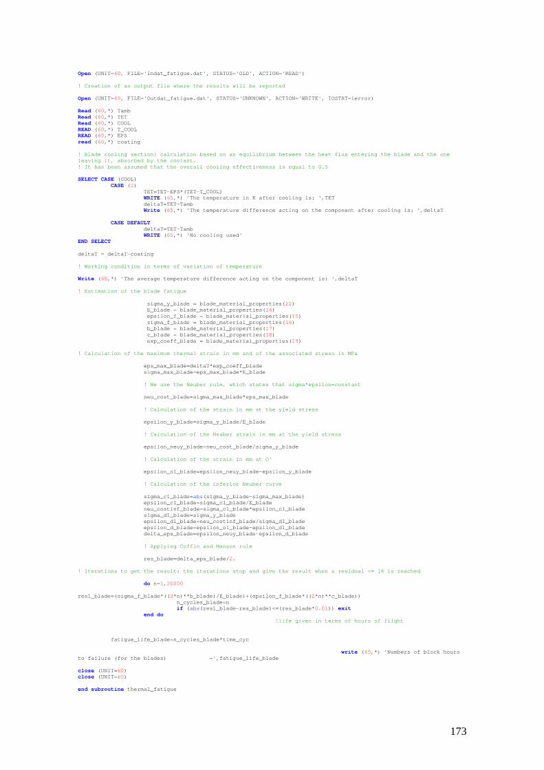
173
Open (UNIT=60, FILE='Indat_fatigue.dat', STATUS='OLD', ACTION='READ')
! Creation of an output file where the results will be reported
Open (UNIT=65, FILE='Outdat_fatigue.dat', STATUS='UNKNOWN', ACTION='WRITE', IOSTAT=ierror)
Read (60,*) TambRead (60,*) TETRead (60,*) COOLREAD (60,*) T_COOLREAD (60,*) EPSread (60,*) coating
! Blade cooling section: calculation based on an equilibrium between the heat flux entering the blade and the oneleaving it, absorbed by the coolant.! It has been assumed that the overall cooling effectiveness is equal to 0.5
SELECT CASE (COOL)CASE (1)
TET=TET-EPS*(TET-T_COOL)WRITE (65,*) 'The temperature in K after cooling is: ',TETdeltaT=TET-TambWrite (65,*) 'The temperature difference acting on the component after cooling is: ',deltaT
CASE DEFAULTdeltaT=TET-TambWRITE (65,*) 'No cooling used'
END SELECT
deltaT = deltaT-coating
! Working condition in terms of variation of temperature
Write (65,*) 'The average temperature difference acting on the component is: ',deltaT
! Estimation of the blade fatigue
sigma_y_blade = blade_material_properties(22)E_blade = blade_material_properties(14)epsilon_f_blade = blade_material_properties(15)sigma_f_blade = blade_material_properties(16)b_blade = blade_material_properties(17)c_blade = blade_material_properties(18)exp_coeff_blade = blade_material_properties(19)
! Calculation of the maximum thermal strain in mm and of the associated stress in MPa
eps_max_blade=deltaT*exp_coeff_bladesigma_max_blade=eps_max_blade*E_blade
! We use the Neuber rule, which states that sigma*epsilon=constant
neu_cost_blade=sigma_max_blade*eps_max_blade
! Calculation of the strain in mm at the yield stress
epsilon_y_blade=sigma_y_blade/E_blade
! Calculation of the Neuber strain in mm at the yield stress
epsilon_neuy_blade=neu_cost_blade/sigma_y_blade
! Calculation of the strain in mm at O'
epsilon_o1_blade=epsilon_neuy_blade-epsilon_y_blade
! Calculation of the inferior Neuber curve
sigma_c1_blade=abs(sigma_y_blade-sigma_max_blade)epsilon_c1_blade=sigma_c1_blade/E_bladeneu_costinf_blade=sigma_c1_blade*epsilon_c1_bladesigma_d1_blade=sigma_y_bladeepsilon_d1_blade=neu_costinf_blade/sigma_d1_bladeepsilon_d_blade=epsilon_o1_blade-epsilon_d1_bladedelta_eps_blade=epsilon_neuy_blade-epsilon_d_blade
! Applying Coffin and Manson rule
res_blade=delta_eps_blade/2.
! Iterations to get the result: the iterations stop and give the result when a residual <= 1% is reached
do n=1,20000
res1_blade=(sigma_f_blade*((2*n)**b_blade)/E_blade)+(epsilon_f_blade*((2*n)**c_blade))n_cycles_blade=nif (abs(res1_blade-res_blade)<=(res_blade*0.01)) exit
end do!life given in terms of hours of flight
fatigue_life_blade=n_cycles_blade*time_cyc
write (65,*) 'Numbers of block hoursto failure (for the blades) =',fatigue_life_blade
close (UNIT=60)close (UNIT=65)
end subroutine thermal_fatigue

174
F.5 Creep Module
! the following subroutine will be able to estimate the creep life of an engine component, by using the larson-millerapproach.it is included also a very simple! mechanism of cooling, where inserting the cooling effectiveness and the coolant temperature as inputs, the newcomponent temperature is calculated. Here in! particular the subroutine is written for a single stage turbine, and allows the user to analyse the blade, the discor both.
subroutine creep (blade_creep_life,blade_material_properties,disk_material_properties)
implicit none
! Declaration of all the variables:double precision :: blade_creep_life,disc_creep_lifeinteger ::nseg,p,q,r,num_t,lmp_check_blade,lmp_type_blade,lmp_constant_blade,lmp_type_disc,lmp_constant_disc,lmp_check_disc,nlmp_blade,nlmp_disc,&& rpm,sf,cool,ierror,blade_stress_select,disc_stress_select,MATERIAL_BLADE,MATERIAL_DISKdouble precision ::temp,time,blade_lmp_value,blade_lmp_stress,blade_lmp,blade_tf,blade_sum_life,blade_total_life,total_time,sigma_max_blade,disc_lmp_value,disc_lmp_stress,&& eps,disc_lmp,disc_tf,disc_sum_life,disc_total_life,sigma_max_disc,sigma_cf,root_cf_load,Coatingdouble precision, allocatable ::t_cool(:),blade_lmp_curve(:,:),disc_lmp_curve(:,:),disc_stress_temp(:,:),blade_stress_temp(:,:),rpm_array(:),temp_array(:),time_array(:)double precision :: blade_material_properties(23),disk_material_properties(23)
! Description of all the variables:! nseg = number of segment into which the flight envelope has been split! sf = rpm of the high pressure turbine first stage at design point! blade_stress_select = stress selector: 1 if the maximum stress acting will be estimated using the blade stresssubroutine, 2 if the maximum stress is inputted by the user! cool = check used to determine whether the blade is cooled or not: 1 if it is, 2 if not! t_cool = temperature in k of the coolant entering the blade! eps = cooling effectiveness! num_t = flight segment time selector: 1 if time is expressed in hours, 2 if it is expressed as percentage of thewhole envelope! total_time = total time spent in flight from the beginning of the simulation! time = time spent during each segment of flight, expressed in hours if num_t = 1, or as a percentage of the wholeflight envelope if num_t = 2! lmp_check_blade = larson-miller parameter selector: 1 if the LMP are unknown and have to be calculated from the LMcurve (inputted by points), 2 if the LMP for each load condition (i.e. segment of flights) are known! lmp_type_blade = larson-miller parameter type selector: 1 if the LM equation is expressed in Imperial Units(temperature in °F and stress in Ksi), 2 if it is expressed in SI (temperature in °K and stress in MPa)! lmp_constant_blade = value of the constant of the LM equation (usually 20 or 25, depending upon the material)! nlmp_blade = number of points of the larson-miller curve known, and that will be inputted to create a curve fromwhere the LMP corresponding to each stress condition will be taken (by interpolation)! blade_lmp = larson-miller parameter for each load condition! cyc_hrs_blade = creep life selector: 1 for creep life in hours, 2 for creep life in cycles (the whole flightenvelope is considered as 1 cycle)! blade_sum_life = sum of all the life fractions of each segment! blade_total_life = total creep life of the blade without safety factors! blade_creep_life = total creep life of the blade with safety factors! disc_stress_select = stress selector: 1 if the maximum stress acting will be estimated using the disc stresssubroutine, 2 if the maximum stress is inputted by the user! lmp_check_disc = larson-miller parameter selector: 1 if the LMP are unknown and have to be calculated from the LMcurve (inputted by points), 2 if the LMP for each load condition (i.e. segment of flights) are known! lmp_type_disc = larson-miller parameter type selector: 1 if the LM equation is expressed in Imperial Units(temperature in °F and stress in Ksi), 2 if it is expressed in SI (temperature in °K and stress in MPa)! lmp_constant_disc = value of the constant of the LM equation (usually 20 or 25, depending upon the material)! nlmp_disc = number of points of the larson-miller curve known, and that will be inputted to create a curve fromwhere the LMP corresponding to each stress condition will be taken (by interpolation)! disc_lmp = larson-miller parameter for each load condition! cyc_hrs_disc = creep life selector: 1 for creep life in hours, 2 for creep life in cycles (the whole flight envelopeis considered as 1 cycle)! disc_sum_life = sum of all the life fractions of each segment! disc_total_life = total creep life of the disc without safety factors! disc_creep_life = total creep life of the disc with safety factors! ierror = indication of an error in the output file! p,q,r = counters used for the loop cycles! num = check used to determine whether the larson-miller parameters will be calculated as an interpolation of atleast 6 values of the curve known, or! they are already known and typed by the user; 1 if there are some curve's values available to interpolate, 2 if theparameters will be inserted as input by the user! nlmp = number of known point of the larson-miller curve, that have to be interpolated the find the current values ofthe larson-miller parameter. this number has to be => 6! cyc_hrs = check used to define wether the user wants a creep life in terms of hours (1) or cycles (2)! stress = values of the stresses acting during each segment of the flight envelope (in mpa), determined fromturbomatch simulations! temp = values of the temperatures acting during each segment of the flight envelope (in k), determined fromturbomatch simulations! time = time spent for each segment of flight (in hours or percentage)! lmp_value = larson-miller parameter known from the curve and interpolated to give the larson-miller parameter weneed! lmp_stress = stresses in mpa correspondant to each larson-miller parameter typed before! lmp = larson-miller parameter acting during each segment of flight. they are already known, so there's no needing tointerpolate! tf = time to failure in hours of each segment of flight, estimated through the larson-miller method! sum_life = sum of the life fractions! total_life = total time to failure of the whole component! total_time = total time (in hours) spent for the whole flight envelope! lmp_curve = matrix that contains the larson-miller parameter and the respective stress associated, that define thelarson-miller curve! stress_temp = matrix that contains all the data we need: stress for each segment, temperature for each segment, timespent for each segment! larson-miller parameter for each segment, time to failure of each segment and total life fraction of each segment! creep_life = creep life in hours of the component! sigma_max_blade = maximum stress acting on the blade
! -------------------opening the input files where data are listed----------------------

175
open (unit=50, file='indat_creep.dat', status='old', action='read')
! --------------------creation of an output file where the results will be reported-----open (unit=55, file='outdat_creep.dat', status='unknown', action='write', iostat=ierror)
! --------------------creep analysis------------------read (50,*) nsegread (50,*) sfread (50,*) blade_stress_selectread (50,*) disc_stress_selectread (50,*) coolread (50,*) epsread (50,*) Coatingread (50,*) lmp_check_bladeread (50,*) lmp_check_disclmp_type_disc=disk_material_properties(23)lmp_constant_disc=disk_material_properties(21)lmp_constant_blade=blade_material_properties(21)lmp_type_blade=blade_material_properties(23)sf=sf*60
allocate (blade_stress_temp(nseg,6)) ! A matrix which will contain all the dataneeded the carry out a creep analysis is created
allocate (rpm_array(nseg),temp_array(nseg),time_array(nseg),t_cool(nseg))
! input stress and temperatures acting during each segment of flight
do p=1,nsegread(50,*) rpm_array(p)
enddo
do p=1,nsegread(50,*) t_cool(p)
enddo
do p=1,nsegread(50,*) temp_array(p)
enddo
do p=1,nsegread(50,*) time_array(p)time_array(p)=time_array(p)/60
enddo
read (50,'(2/)')
do p=1,nsegselect case (blade_stress_select)
case (1)rpm=rpm_array(p)*sf
! The rpm is the needed input file to use the blade stress subroutinecall blade_stress
(rpm,sigma_max_blade,root_cf_load,blade_material_properties)case (2)
read (50,*) sigma_max_bladeend selectblade_stress_temp(p,1)=sigma_max_blade
! The first coloumn of the matrix contains the stresses acting during each segment of flightblade_stress_temp(p,2)=temp_array(p) ! The second
coloumn of the matrix contains the maximum temperature acting during each segment of flightend do
! -------------------cooling section------------------! calculation based on an equilibrium between the heat flux entering the blade and the one leaving
it, absorbed by the coolant.
select case (cool)case (1)! calculation of the new temperature of the metal after cooling:
do p=1,nsegblade_stress_temp(p,2)=blade_stress_temp(p,2)-
eps*(blade_stress_temp(p,2)-t_cool(p))end do
case (2) ! no coolingwrite (55,*) 'no cooling used'
end select! ----------------------end of the blade cooling section------------------
!--------------------------Effect of thermal barrier coating---------------------
do p=1,nsegblade_stress_temp(p,2)=blade_stress_temp(p,2)-Coating
end do
! ---------------------input of time spent for each flight segment--------
total_time=0 ! inizialization of the variabledo p=1,nseg
blade_stress_temp(p,3)=time_array(p) ! Thethird coloumn of the matrix contains the amount of time spent during each segment of flight
total_time=total_time+blade_stress_temp(p,3)end do
! -------------------------calculation of the larson-miller parameter--------------------
if (lmp_check_blade==1) thennlmp_blade = 6allocate (blade_lmp_curve(nlmp_blade,2))
! A matrix containing the LMP and their respective stresses is created! values of the larson-miller parameter available(at least 6), with the corresponding stress
value, read from the input file:

176
! IMPORTANT!! The known Larson-miller parameters have to be inserted in a decreasing order, fromthe higher to the lower!
blade_lmp_curve(1,1)=blade_material_properties(1) ! first coloumn of the matrixcontaining the LMP
blade_lmp_curve(2,1)=blade_material_properties(3)
blade_lmp_curve(3,1)=blade_material_properties(5)
blade_lmp_curve(4,1)=blade_material_properties(7)
blade_lmp_curve(5,1)=blade_material_properties(9)
blade_lmp_curve(6,1)=blade_material_properties(11)
blade_lmp_curve(1,2)=blade_material_properties(2) ! second coloumn of the matrixcontaining the stress
blade_lmp_curve(2,2)=blade_material_properties(4)blade_lmp_curve(3,2)=blade_material_properties(6)blade_lmp_curve(4,2)=blade_material_properties(8)blade_lmp_curve(5,2)=blade_material_properties(10)blade_lmp_curve(6,2)=blade_material_properties(12)
! interpolation of the available larson-miller curve to get the larson-miller parameter for stresscondition (i.e. each segment of flight)
select case (lmp_type_blade)case (1)
! LM equation in Imperial Unitsdo p=1,nseg
blade_stress_temp(p,1)=blade_stress_temp(p,1)/6.894 ! Stress converted from MPa to Ksi, as the Larson-Miller curve is given in Imperial Units
blade_stress_temp(p,2)=blade_stress_temp(p,2)-273.15
blade_stress_temp(p,2)=(blade_stress_temp(p,2)*9./5.)+32. ! Temperatures in farenightend doouter: do p=1,nseg
inner: do q=1,nlmp_blade-1
blade_lmp=0if
(blade_stress_temp(p,1)>=blade_lmp_curve(q,2).and.blade_stress_temp(p,1)<=blade_lmp_curve(q+1,2)) then
blade_lmp=blade_lmp_curve(q+1,1)+(blade_lmp_curve(q,1)-blade_lmp_curve(q+1,1))*(blade_lmp_curve(q+1,2)-blade_stress_temp(p,1))/(blade_lmp_curve(q+1,2)-blade_lmp_curve(q,2))
elseif(blade_stress_temp(p,1)<blade_lmp_curve(1,2)) then
blade_lmp=blade_lmp_curve(1,1)
elseif(blade_stress_temp(p,1)>blade_lmp_curve(nlmp_blade,2)) then
blade_lmp=blade_lmp_curve(nlmp_blade,1)
endif! calculation of time to failure
for each segment (in hours)
blade_tf=10**(blade_lmp*1000/(blade_stress_temp(p,2)+460)-lmp_constant_blade)blade_stress_temp(p,4)=blade_lmp
! fourth coloumn of the matrix containing the LMP corresponding to the loadcondition
blade_stress_temp(p,5)=blade_tf! fifth coloumn of the matrix
containing the time to failure corresponding to each load condition
blade_stress_temp(p,6)=blade_stress_temp(p,3)/blade_tf ! sixth coloumn containing the life fraction ofeach load condition
if (blade_lmp/=0) exitend do inner
end do outercase (2)
! LM equation in SIdo p=1,nsegdo q=1,nlmp_blade
blade_lmp=0if
(blade_stress_temp(p,1)>=blade_lmp_curve(q,2).and.blade_stress_temp(p,1)<=blade_lmp_curve(q+1,2)) then
blade_lmp=blade_lmp_curve(q+1,1)+(blade_lmp_curve(q,1)-blade_lmp_curve(q+1,1))*(blade_lmp_curve(q+1,2)-blade_stress_temp(p,1))/(blade_lmp_curve(q+1,2)-blade_lmp_curve(q,2))
elseif(blade_stress_temp(p,1)<blade_lmp_curve(1,2)) then
blade_lmp=blade_lmp_curve(1,1)
elseif(blade_stress_temp(p,1)>blade_lmp_curve(nlmp_blade,2)) then
blade_lmp=blade_lmp_curve(nlmp_blade,1)endif
blade_stress_temp(p,4)=blade_lmp ! fourth coloumn of the matrixcontaining the LMP corresponding to the load condition

177
! calculation of time to failure for each segment (in hours)
blade_tf=10**(blade_lmp*1000/blade_stress_temp(p,2)-lmp_constant_blade)
blade_stress_temp(p,5)=blade_tf! fifth coloumn of the matrix containing the time to failure corresponding to each load condition
blade_stress_temp(p,6)=blade_stress_temp(p,3)/blade_tf ! sixth coloumn containing the lifefraction of each load condition
if (blade_lmp/=0) exitend do
end doend select
else if (lmp_check_blade==2) then ! larson-miller parameter already known for eachsegment and introduced by the user through the input file
do p=1,nseg ! larson-miller parameter acting on each segment of flight,read from the input file
read (50,*) blade_lmpblade_stress_temp(p,4)=blade_lmp
! calculation of time to failure for each segment (in hours)select case (lmp_type_blade)
case (1) ! LM equation in Imperial Unitsblade_stress_temp(p,1)=blade_stress_temp(p,1)/6.894blade_stress_temp(p,2)=blade_stress_temp(p,2)-273.15
blade_stress_temp(p,2)=(blade_stress_temp(p,2)*9./5.)+32. ! Temperatures in farenight
blade_tf=10**(blade_lmp*1000/(blade_stress_temp(p,2)+460)-lmp_constant_blade)case (2) ! LM equation in
SI
blade_tf=10**(blade_lmp*1000/blade_stress_temp(p,2)-lmp_constant_blade)end select
blade_stress_temp(p,5)=blade_tfblade_stress_temp(p,6)=blade_stress_temp(p,3)/blade_tf
end doend if
! -------------------------------calculation of creep life using the cumulative Miner'slaw----------------------------------! first of all, it is to be decided wether to estimate the creep life in hours or cycles; talking about cycles, weassume that the sum of all the segments of! flight (i.e. the whole flight envelope) represents 1 cycle through the variable cyc_hrs, read from the input file,it is decided whether we want the creep life! in hours (cyc_hrs = 1) or in cycles (cyc_hrs = 2)
! creep life in hoursblade_sum_life=0 !
inizialization of the variabledo r=1,nseg
blade_sum_life=blade_sum_life+blade_stress_temp(r,6)end doblade_total_life=total_time/blade_sum_life
blade_creep_life=blade_total_life ! total creep life of the component
write (55,*) 'total blade creep life=',blade_creep_life, 'hrs'
write (55,*)if (lmp_type_blade==1) then
do p=1,nsegblade_stress_temp(p,1)=blade_stress_temp(p,1)*6.894 ! Stress converted from MPa to Ksi, as the Larson-
Miller curve is given in Imperial Unitsblade_stress_temp(p,2)=(blade_stress_temp(p,2)-32.)*5./9. ! Temperatures in farenightblade_stress_temp(p,2)=blade_stress_temp(p,2)+273.15
end doend if
write (55,110) 'Blade Stress (MPa) ',blade_stress_temp(:,1)write (55,110) 'Blade Temperature (K) ',blade_stress_temp(:,2)write (55,110) 'Blade Time spent (hrs) ',blade_stress_temp(:,3)write (55,110) 'Blade LMP ',blade_stress_temp(:,4)write (55,120) 'Blade Time to failure (hrs) ',blade_stress_temp(:,5)write (55,130) 'Blade Life fraction ',blade_stress_temp(:,6)
!****************************************************************************************************************
! disk creep calculations
allocate (disc_stress_temp(nseg,6)) ! A matrix whichwill contain all the data needed the carry out a creep analysis is created
! input stress and temperatures acting during each segment of flight
do p=1,nsegselect case (disc_stress_select)
case (1)rpm=rpm_array(p)*sf
! The rpm is the needed input file to use the disc stress subroutinecall disc_stress
(rpm,sigma_max_disc,sigma_cf,sigma_max_blade,disk_material_properties,blade_material_properties)case default
read (50,*) sigma_max_discend selectdisc_stress_temp(p,1)=sigma_max_disc ! The first coloumn of the
matrix contains the stresses acting during each segment of flightdisc_stress_temp(p,2)=temp_array(p)
! The second coloumn of the matrix contains the maximum temperature acting during each segment of flightend do
! ---------------------input of time spent for each flight segment--------

178
total_time=0 ! inizialization of the variabledo p=1,nseg
disc_stress_temp(p,3)=time_array(p)! The third coloumn of the matrix contains the amount of time spent during each segment of flight
total_time=total_time+disc_stress_temp(p,3)end do
! -------------------------calculation of the larson-miller parameter--------------------
if (lmp_check_disc==1) thennlmp_disc = 6allocate (disc_lmp_curve(nlmp_disc,2)) ! A
matrix containing the LMP and their respective stresses is created
! values of the larson-miller parameter available(at least6), with the corresponding stress value, read from the input file:
! IMPORTANT!! The known Larson-miller parameters have tobe inserted in a decreasing order, from the higher to the lower!
disc_lmp_curve(1,1)=disk_material_properties(1)! first coloumn of the matrix containing the LMP
disc_lmp_curve(2,1)=disk_material_properties(3)disc_lmp_curve(3,1)=disk_material_properties(5)disc_lmp_curve(4,1)=disk_material_properties(7)disc_lmp_curve(5,1)=disk_material_properties(9)disc_lmp_curve(6,1)=disk_material_properties(11)
disc_lmp_curve(1,2)=disk_material_properties(2)! second coloumn of the matrix containing the stress
disc_lmp_curve(2,2)=disk_material_properties(4)disc_lmp_curve(3,2)=disk_material_properties(6)disc_lmp_curve(4,2)=disk_material_properties(8)disc_lmp_curve(5,2)=disk_material_properties(10)disc_lmp_curve(6,2)=disk_material_properties(12)
! interpolation of the available larson-miller curve to get the larson-miller parameter for stress condition(i.e. each segment of flight)
select case (lmp_type_disc)case (1)
! LM equation in Imperial Unitsdo p=1,nseg
disc_stress_temp(p,1)=disc_stress_temp(p,1)/6.894 ! Stress converted from MPa to Ksi, as the Larson-Miller curve isgiven in Imperial Units
disc_stress_temp(p,2)=disc_stress_temp(p,2)-273.15
disc_stress_temp(p,2)=(disc_stress_temp(p,2)*9./5.)+32.end do
do p=1,nsegdo q=1,nlmp_discdisc_lmp=0
if(disc_stress_temp(p,1)>=disc_lmp_curve(q,2).and.disc_stress_temp(p,1)<=disc_lmp_curve(q+1,2)) then
disc_lmp=disc_lmp_curve(q+1,1)+(disc_lmp_curve(q,1)-disc_lmp_curve(q+1,1))*(disc_lmp_curve(q+1,2)-disc_stress_temp(p,1))/(disc_lmp_curve(q+1,2)-disc_lmp_curve(q,2))
else if(disc_stress_temp(p,1)<disc_lmp_curve(1,2))then
disc_lmp=disc_lmp_curve(1,1)else if
(disc_stress_temp(p,1)>disc_lmp_curve(nlmp_disc,2)) then
disc_lmp=disc_lmp_curve(6,1)end if
disc_stress_temp(p,4)=disc_lmp ! fourth coloumn of the matrixcontaining the LMP corresponding to the load condition
! calculation of time to failure for each segment (in hours)
disc_tf=10**(disc_lmp*1000/(disc_stress_temp(p,2)+460)-lmp_constant_disc)
disc_stress_temp(p,5)=disc_tf ! fifthcoloumn of the matrix containing the time to failure corresponding to each load condition
disc_stress_temp(p,6)=disc_stress_temp(p,3)/disc_tf ! sixth coloumn containing the lifefraction of each load condition
if (disc_lmp/=0)exit
end doend do
case (2)! LM equation in SI
do p=1,nsegdo q=1,nlmp_discdisc_lmp=0
if(disc_stress_temp(p,1)>=disc_lmp_curve(q,2).and.disc_stress_temp(p,1)<=disc_lmp_curve(q+1,2)) then
disc_lmp=disc_lmp_curve(q+1,1)+(disc_lmp_curve(q,1)-disc_lmp_curve(q+1,1))*(disc_lmp_curve(q+1,2)-disc_stress_temp(p,1))/(disc_lmp_curve(q+1,2)-disc_lmp_curve(q,2))
else if(disc_stress_temp(p,1)<disc_lmp_curve(1,2)) then
disc_lmp=disc_lmp_curve(1,1)else if
(disc_stress_temp(p,1)>disc_lmp_curve(nlmp_disc,2)) then

179
disc_lmp=disc_lmp_curve(6,1)end if
disc_stress_temp(p,4)=disc_lmp ! fourth coloumn of the matrixcontaining the LMP corresponding to the load condition
! calculation of time to failure for each segment (in hours)
disc_tf=10**(disc_lmp*1000/disc_stress_temp(p,2)-lmp_constant_disc)
disc_stress_temp(p,5)=disc_tf ! fifthcoloumn of the matrix containing the time to failure corresponding to each load condition
disc_stress_temp(p,6)=disc_stress_temp(p,3)/disc_tf ! sixth coloumn containing the lifefraction of each load condition
if (disc_lmp/=0) exitend do
end doend select
else if (lmp_check_disc==2) then ! larson-miller parameter already known for eachsegment and introduced by the user through the input file
do p=1,nseg! larson-miller parameter acting on each segment of flight, read from the input file
read (50,*) disc_lmpdisc_stress_temp(p,4)=disc_lmp
! calculation of time to failure for each segment (in hours)select case (lmp_type_disc)
case (1) ! LM equation in Imperial Unitsdisc_stress_temp(p,1)=disc_stress_temp(p,1)/6.894 !
Stress converted from MPa to Ksi, as the Larson-Miller curve is given in Imperial Unitsdisc_stress_temp(p,2)=disc_stress_temp(p,2)-
273.15
disc_stress_temp(p,2)=(disc_stress_temp(p,2)*9./5.)+32.
disc_tf=10**(disc_lmp*1000/(disc_stress_temp(p,2)+460)-lmp_constant_disc)
case (2) ! LM equation in SI
disc_tf=10**(disc_lmp*1000/disc_stress_temp(p,2)-lmp_constant_disc)end select
disc_stress_temp(p,5)=disc_tfdisc_stress_temp(p,6)=disc_stress_temp(p,3)/disc_tf
end doend if
! -------------------------------calculation of creep life using the cumulative Miner's law----------------------------------! first of all, it is to be decided wether to estimate the creep life in hours or cycles; talking about cycles,
! we assume that the sum of all the segments of flight (i.e. the whole flight envelope)represents 1 cycle! through the variable cyc_hrs, read from the input file, it is decided whether we want the creep life in hours(cyc_hrs = 1) or in cycles (cyc_hrs = 2)
! creep life in hoursdisc_sum_life=0 !
inizialization of the variabledo r=1,nseg
disc_sum_life=disc_sum_life+disc_stress_temp(r,6)end dodisc_total_life=total_time/disc_sum_life
disc_creep_life=disc_total_life ! total creep life of the componentwrite (55,*)
write (55,*) 'total disc creep life=',disc_creep_life, 'hrs'
write (55,*)if (lmp_type_disc==1) then
do p=1,nsegdisc_stress_temp(p,1)=disc_stress_temp(p,1)*6.894 ! Stress converted from MPa to Ksi, as the Larson-Miller
curve is given in Imperial Unitsdisc_stress_temp(p,2)=(disc_stress_temp(p,2)-32.)*5./9.disc_stress_temp(p,2)=disc_stress_temp(p,2)+273.15
end doend if
write (55,110) 'Disc Stress (MPa) ',disc_stress_temp(:,1)write (55,110) 'Disc Temperature (K) ',disc_stress_temp(:,2)write (55,110) 'Disc Time spent (hrs) ',disc_stress_temp(:,3)write (55,110) 'Disc LMP ',disc_stress_temp(:,4)write (55,120) 'Disc Time to failure (hrs) ',disc_stress_temp(:,5)write (55,130) 'Disc Life fraction ',disc_stress_temp(:,6)
! --------------------end of creep analysis------------------
! -------------------closing the input and output units------------------------------close (unit=50)close (unit=55)
! --------------------------outputs format-----------------------------110 format (' ',A30,5(F10.2,10X))120 format (' ',A30,F10.2,10X,F10.2,10X,F10.2,11X,F12.2,7X,F10.2,10X)130 format (' ',A30,F10.8,10X,F10.8,10X,F10.8,11X,F12.8,7X,F10.8,10X)end subroutine creep

180
F.6 Disk Stress Module
! The following subroutine will be able to estimate the maximum stress acting on the disc of a turbine stage: the discto be! analysed can be a constant thickness or a varying thickness one: a subroutine is needed to proceed solving a linearsystem! of equations.
subroutine disc_stress(rpm,sigma_max_disc,sigma_cf,sigma_max_blade,disk_material_properties,blade_material_properties)
implicit none
! Variables declarationinteger, intent(in) :: rpmdouble precision, intent(out) :: sigma_max_disc,sigma_cf,sigma_max_bladedouble precision ::rim_dia,bore_dia,thick,sigma_r_bore,sigma_h_bore,sigma_r_rim,sigma_h_rim,sigma_eq_rim,rim_radial_stress,blade_mass,in_rad,out_rad,blade_cg_rad,rim_area,&& root_cf_load,omega,ro_disc,nuinteger :: istat,i,j,n,const_thick,n_ring,check,rim_stress,n_bladesinteger, parameter :: n_eq=6 ! maximum number of equations to solve in a linear system (using a subroutineincluded)double precision, parameter :: pi=3.1415926double precision, parameter :: iter=10000.double precision, dimension(n_eq,n_eq) :: adouble precision, dimension(n_eq) :: binteger :: errordouble precision, allocatable ::inner_radius(:,:),outer_radius(:,:),thickness(:,:),sigma_h_in(:,:),sigma_r_in(:,:),S_in(:,:),S_out(:,:),D_in(:,:),D_out(:,:),&& sigma_h_out(:,:),sigma_r_out(:,:),delta_sigma_r(:,:),delta_sigma_h(:,:),von_mises(:,:)double precision :: disk_material_properties(23),blade_material_properties(23)
! Description of all the variables:! nu = Poisson's ratio of the disc material! ro_disc = density of the disc material (in Kg/m^3)! const_thick = disc type selector: 1 if the disc is a constant thickness type, 2 if it is a varying thickness one! rim_stress = rim stress selector: 1 if the centrifugal load is unknown and has to be calculated using the bladestress subroutine, 2 if it is calculated knowing blade mass and radius of blade centre of gravity, 3 if the rim stressis already given as input! omega = angular velocity in rad/s! n = number of equations to be solved in the linear system! rim_dia = rim diameter (m) of the constant thickness disc! bore_dia = bore diameter (m) of the constant thickness disc! thick = thickness (m) of the constant thickness disc (or of each ring the varying thickness disc has beendiscretised into)! n_blades = number of blades carried by the disc! rim_area = area of the disc (m^2) over which the centrifugal stress due to the presence of the blades is spread! root_cf_load = centrifugal load of one blade (MN)! sigma_cf = rim stress! blade_mass = mass of a blade (Kg)! blade_cg_rad = radius of the centre of gravity of the blade (m)! rim_radial_stress = sigma_cf = rim radial stress! sigma_r_bore = radial stress at the bore! sigma_r_rim = radial stress at the rim! sigma_h_bore = hoop stress at the bore! sigma_h_rim = hoop stress at the rim! sigma_eq_rim = von mises stress at the rim, obtained combining the hoop and the radial stress at the rim! sigma_max_disc = maximum stress acting on the disc! n_ring = number of rings into which the! inner_radius = matrix containing the inner radius (m) of each ring the varying thickness disc has been discretisedinto! outer_radius = matrix containing the outer radius (m) of each ring the varying thickness disc has been discretisedinto! thickness = matrix containing the thickness (m) of each ring the varying thickness disc has been discretised into! in_rad = inner radius (m) of each ring the varying thickness disc has been discretised into! von_mises = equivalent von mises stress calculated combining the hoop and radial stress at each station
! -------------------opening the input file where data are listed------------------------------open (unit=1,file='disc_input.dat',status='old',action='read',iostat=istat)
! -------------------creation of the output file where the results will be written------------------------------open (unit=2,file='disc_output.dat',status='unknown',action='write',iostat=istat)
nu = disk_material_properties(20)ro_disc = disk_material_properties(13)read (1,*) const_thickread (1,*) rim_stressread (1,*) rim_diaread (1,*) bore_diaread (1,*) thickread (1,*) n_blades
omega=(rpm/60.)*2*pi ! rpm transformed into angular velocity (rad/s)
!------------------Constant thickness hollow disc------------------
select case (const_thick)case (1) ! Constant Thickness disc
n=2 ! number of equations to solve withthe subroutine
select case (rim_stress)case (1) ! Rim stress to be calculated using
the blade stress subroutinecall blade_stress (rpm,sigma_max_blade,root_cf_load,blade_material_properties)rim_area=pi*rim_dia*thicksigma_cf=root_cf_load*n_blades/rim_area
case (2) ! Rim stress to be calculated knowingnumber of blades, balde mass and radius of the centre of gravity

181
read (1,*) blade_massread (1,*) blade_cg_radrim_area=pi*rim_dia*thicksigma_cf=n_blades*blade_mass*blade_cg_rad*omega**2/rim_area
case (3)read (1,*) sigma_cf
end select
rim_radial_stress=sigma_cf
! Coefficient (a) and right-hand side (b) of the linear system of equationa(1,1)=1a(1,2)=-1./((bore_dia/2.)**2.)b(1)=(3.+nu)*ro_disc*(omega**2)*((bore_dia/2.)**2.)/8.a(2,1)=1a(2,2)=-1./((rim_dia/2.)**2.)b(2)=(sigma_cf*10**6)+((3.+nu)*ro_disc*(omega**2)*((rim_dia/2.)**2.)/8.)
! Solve equations (using the subroutine provided)call simul (a,b,n_eq,n,error)do i=1,n
write (2,*) 'solution of equation',i,' = ',b(i) ! The solutions ofthe equations are written
end do
sigma_r_bore=0sigma_r_rim=sigma_cfsigma_h_bore=(b(1)+b(2)/((bore_dia/2.)**2.)-
((1+3*nu)*ro_disc*(omega**2)*((bore_dia/2.)**2.)/8.))/10.**6sigma_h_rim=(b(1)+b(2)/((rim_dia/2.)**2.)-
((1+3*nu)*ro_disc*(omega**2)*((rim_dia/2.)**2.)/8.))/10.**6
! Combination of the hoop and radial stress acting at the rim, using Von Mises equationsigma_eq_rim=1/(sqrt(2.))*sqrt((sigma_h_rim-sigma_r_rim)**2.+(sigma_r_rim-0)**2.+(0-
sigma_h_rim)**2.)
write (2,*) 'sigma_r_bore =',sigma_r_borewrite (2,*) 'sigma_r_rim =',sigma_r_rimwrite (2,*) 'sigma_h_bore =',sigma_h_borewrite (2,*) 'sigma_h_rim =',sigma_h_rimwrite (2,*) 'sigma_eq_rim =',sigma_eq_rim
! Comparison of the stresses in order to get the maximum acting on the discif (sigma_r_bore>=sigma_h_bore) then
sigma_max_disc=sigma_r_boreelse
sigma_max_disc=sigma_h_boreend if
if (sigma_max_disc>=sigma_eq_rim) thensigma_max_disc=sigma_max_disc
elsesigma_max_disc=sigma_eq_rim
end if
!------------------Varying thickness hollow disc------------------
case (2)n=6 ! number of equations to be solvedread (1,*) n_ring
allocate(inner_radius(n_ring+1,1),outer_radius(n_ring,1),thickness(n_ring+1,1),sigma_h_in(n_ring+1,1000000),sigma_r_in(n_ring+1,1000000),&&von_mises(n_ring+1,1000000),S_in(n_ring+1,1000000),S_out(n_ring,1000000),D_in(n_ring+1,1000000),D_out(n_ring,1000000),sigma_h_out(n_ring,1000000),&& sigma_r_out(n_ring,1000000),delta_sigma_r(n_ring,1000000),delta_sigma_h(n_ring,1000000))
do i=1,n_ring+1read (1,*) in_radinner_radius(i,1)=in_radread (1,*) thickthickness(i,1)=thick
end do
do j=1,n_ringouter_radius(j,1)=inner_radius(j+1,1)
end do
select case (rim_stress)case (1) ! Rim stress to be calculated using the blade stress subroutine
call blade_stress (rpm,sigma_max_blade,root_cf_load,blade_material_properties)rim_area=pi*rim_dia*thicksigma_cf=root_cf_load*n_blades/rim_area
case (2) ! Rim stress to be calculated knowingnumber of blades, balde mass and radius of the centre of gravity
read (1,*) blade_massread (1,*) blade_cg_radrim_area=pi*rim_dia*thicksigma_cf=n_blades*blade_mass*blade_cg_rad*omega**2/rim_area
case (3)read (1,*) sigma_cf
end select
rim_radial_stress=sigma_cf
! Boundary conditions: bore radial stress = 0 and bore hoop stress guessed to be = 100 MPasigma_h_in(1,1)=100.*10**6sigma_r_in(1,1)=0.S_in(1,1)=sigma_h_in(1,1)D_in(1,1)=S_in(1,1)

182
! Iterations needed to get a calculated rim radial stress equal to the actual value of itdo j=1,iter
do i=1,n_ring! Coefficient of the linear system to be solveda(1,1)=1.a(1,2)=0.a(1,3)=-1./2.a(1,4)=-1./2.a(1,5)=0.a(1,6)=0.a(2,1)=0.a(2,2)=1.a(2,3)=-1./2.a(2,4)=1./2.a(2,5)=0.a(2,6)=0.a(3,1)=0.a(3,2)=0.a(3,3)=1.a(3,4)=0.a(3,5)=0.a(3,6)=0.a(4,1)=0.a(4,2)=0.a(4,3)=0.a(4,4)=1.a(4,5)=0.a(4,6)=0.a(5,1)=0.a(5,2)=-(thickness(i,1)/thickness(i+1,1)-1)a(5,3)=0.a(5,4)=0.a(5,5)=1.a(5,6)=0.a(6,1)=0.a(6,2)=0.a(6,3)=0.a(6,4)=0.a(6,5)=-nua(6,6)=1.
! Right-hand side of the linear system of equations to be solvedb(1)=0.b(2)=0.b(3)=S_in(i,j)-((1.+nu)/2.)*ro_disc*(omega**2)*(outer_radius(i,1)**2-
inner_radius(i,1)**2)b(4)=D_in(i,j)*(inner_radius(i,1)**2/outer_radius(i,1)**2)-(1.-
nu)*ro_disc*(omega**2)*(inner_radius(i,1)**4/outer_radius(i,1)**2-outer_radius(i,1)**2)/4.b(5)=0.b(6)=0.
call simul (a,b,n_eq,n,error)
! Results got from the system of linear equations
sigma_h_out(i,j)=b(1)sigma_r_out(i,j)=b(2)S_out(i,j)=b(3)D_out(i,j)=b(4)delta_sigma_r(i,j)=b(5)delta_sigma_h(i,j)=b(6)sigma_h_in(i+1,j)=sigma_h_out(i,j)+delta_sigma_h(i,j)sigma_r_in(i+1,j)=sigma_r_out(i,j)+delta_sigma_r(i,j)S_in(i+1,j)=sigma_h_in(i+1,j)+sigma_r_in(i+1,j)D_in(i+1,j)=sigma_h_in(i+1,j)-sigma_r_in(i+1,j)
end do
check=j! Check of the results: the iterations stop when the estimated rim radial stress differs
from the actual value for 0.001%if ((abs((sigma_r_in(n_ring+1,j)-rim_radial_stress*10**6))<=rim_radial_stress*10) .and.
sigma_r_in(n_ring+1,j)>=0.) exit
sigma_h_in(1,j+1)=sigma_h_in(1,j)+1000.sigma_r_in(1,j+1)=0.S_in(1,j+1)=sigma_h_in(1,j+1)D_in(1,j+1)=S_in(1,j+1)
end do
! Results converted into MPasigma_h_in=sigma_h_in/10**6sigma_r_in=sigma_r_in/10**6
! Equivalent von mises stress calculationif (check<1000000.) then
do i=1,n_ringvon_mises(i,check)=(1./sqrt(2.))*sqrt((sigma_h_in(i,check)-
sigma_r_in(i,check))**2+(sigma_r_in(i,check)-0)**2+(0-sigma_h_in(i,check))**2)write (2,*) 'sigma (h_in,r_in,von_mises) =
',sigma_h_in(i,check),sigma_r_in(i,check),von_mises(i,check)end do
sigma_max_disc=0.
! Maximum stress identificationdo i=1,n_ring
if (sigma_max_disc < von_mises(i,check)) thensigma_max_disc = von_mises(i,check)write (2,*) 'von mises sigma max =',sigma_max_disc
elsesigma_max_disc = sigma_max_discwrite (2,*) 'sigma max =',sigma_max_disc
end if

183
end doelse
write (2,*) 'no convergence'end if
end select
close (unit=1)close (unit=2)
end subroutine disc_stress
!--------------------------------------------------------------------------------------------------------------------------------------
subroutine simul (a,b,ndim,n,error)
! Purpose: subroutine to solve a set of n linear equations in n unknowns using Gaussian elimination and the maximumpivot technique
implicit none
! Data dictionary: declare calling parameters types & definitionsinteger, intent(in) :: ndim !dimension of arrays a and bdouble precision, intent(inout), dimension(ndim,ndim) :: a ! Array of coefficient (n xn). This array is of size ndim x ndim, but only n x n of the coefficients are being used. The declare dimension mustbe passed to the subroutine or it won't be able to interpret subscripts correctly. (This array is destroyed duringprocessing)double precision, intent(inout), dimension(ndim) :: b ! input: right-hand side of equations.
! output: solution vector
integer, intent(in) :: n ! numberof equations to solveinteger, intent(out) :: error ! error flag: 0 noerror, 1 singular equations
! Data dictionary: declare constantsdouble precision, parameter :: epsilon = 1.0D-6 ! a"small" number for comparison when determining singular equations
! Data dictionary: declare local variable types and definitionsdouble precision :: factor
! factor to multiply equation i-row by, before adding to equation j-rowinteger :: irow
! number of the equation currently being processedinteger :: ipeak
! pointer to equation containing maximum pivot valueinteger :: jrow
! number of the equation compared to the current equationinteger :: kcol
! index over all columns of euqationsdouble precision :: temp
! scratch value
! Process n times to get all equations....mainloop: do irow=1,n
! Find peak pivot for column irow in rows irow to nipeak=irowmax_pivot: do jrow=irow+1,n
if (abs(a(jrow,irow))>abs(a(ipeak,irow))) thenipeak=jrow
end ifend do max_pivot
! Check for singular equations.singular: if (abs(a(ipeak,irow))<epsilon) then
error=1return
end if singular
! Otherwise, if ipeak/= irow, swap equations irow and ipeakswap_eqn: if (ipeak/=irow) then
do kcol=1,ntemp=a(ipeak,kcol)a(ipeak,kcol)=a(irow,kcol)a(irow,kcol)=temp
end dotemp=b(ipeak)b(ipeak)=b(irow)b(irow)=temp
end if swap_eqn
! Multiply equation irow by -a(jrow,irow)/a(irow,irow), and add it to Eqn jrow (for all eqns except irowitself)
eliminate: do jrow=1,nif (jrow/=irow) then
factor=-a(jrow,irow)/a(irow,irow)do kcol=1,n
a(jrow,kcol)=a(irow,kcol)*factor+a(jrow,kcol)end dob(jrow)=b(irow)*factor+b(jrow)
end ifend do eliminate
end do mainloop
! End of main loop over all equations. All off-diagonal terms are now zero. To get the final answer, we must divideeach! equations by the coefficient of its non-diagonal termdivide: do irow=1,n
b(irow)=b(irow)/a(irow,irow)

184
a(irow,irow)=1end do divide
! Set error flag to 0 and returnerror=0
end subroutine simul
F.7 Blade Stess Module
!--------------------------Blade Stress Calculation using centrifugal forces only-------
subroutine blade_stress (rpm,sigma_max_blade,root_cf_load,blade_material_properties)
implicit none
integer, intent(in) :: rpmdouble precision, intent(out) :: sigma_max_bladedouble precision, intent(out) :: root_cf_loaddouble precision :: ro_blade,omega,An,rad,area,sigma_cf,sigma_cf_approxdouble precision,parameter :: pi=3.1415926double precision,allocatable :: radius(:,:)double precision,allocatable ::cross_area(:,:),mean_cross_area(:,:),sec_height(:,:),volume(:,:),mass(:,:),cg_radius(:,:),sec_cf_load(:,:),tot_cf_load(:,:),cf_stress(:,:)double precision :: blade_material_properties(23)integer :: n_sec,t
open (40,file='blade_stress_input.dat',status='unknown',action='read')open (45,file='blade_stress_output.dat',status='unknown',action='write')
read (40,*) n_secro_blade = blade_material_properties(13)
omega=(rpm/60.)*2.*pi
allocate(radius(n_sec+1,1),cross_area(n_sec+1,1),mean_cross_area(n_sec,1),sec_height(n_sec,1),volume(n_sec,1),mass(n_sec,1),cg_radius(n_sec,1),&& sec_cf_load(n_sec,1),tot_cf_load(n_sec+1,1),cf_stress(n_sec+1,1))
do t=1,n_sec+1read (40,*) radradius(t,1)=rad
end do
do t=1,n_sec+1read (40,*) areacross_area(t,1)=area
end do
do t=1,n_secmean_cross_area(t,1)=(cross_area(t,1)+cross_area(t+1,1))/2.sec_height(t,1)=radius(t+1,1)-radius(t,1)volume(t,1)=mean_cross_area(t,1)*sec_height(t,1)mass(t,1)=volume(t,1)*ro_bladecg_radius(t,1)=(radius(t+1,1)+radius(t,1))/2.sec_cf_load(t,1)=mass(t,1)*cg_radius(t,1)*omega**2
end do
do t=n_sec+1,2,-1tot_cf_load(n_sec+1,1)=0
tot_cf_load(t-1,1)=sec_cf_load(t-1,1)+tot_cf_load(t,1)end do
do t=1,n_sec+1cf_stress(t,1)=(tot_cf_load(t,1)/cross_area(t,1))/1000000.
end do
sigma_cf=cf_stress(1,1)root_cf_load=tot_cf_load(1,1)/1000000.An=pi*(radius(n_sec+1,1)**2.-radius(1,1)**2.)
! approximate estimate of the maximum centrifugal stress at the root
sigma_cf_approx=(2.*pi*((rpm/60.)**2.)*ro_blade*An)/1000000. !maximumcentrifugal force that occurs at the blade root
write (45,*) 'sec_cf_load = ',sec_cf_loadwrite (45,*) 'tot_cf_load =',tot_cf_loadwrite (45,*) 'cf_stress =',cf_stresswrite (45,*) 'sigma_cf =',sigma_cfwrite (45,*) 'sigma_cf_approx =',sigma_cf_approx
sigma_max_blade=sigma_cf_approx
close (unit=40)close (unit=45)
end subroutine blade_stress