Daniel Kroening and Ofer Strichman

Decision ProceduresAn Algorithmic Point of View

Gaussian Elimination andSimplex

Gaussian’s elimination

Given a linear system Ax = b

Manipulate A|b to an upper-triangular form

A x = b

Gaussian’s elimination

Then, solve backwards from the k’s row according to:

Gaussian elimination - example

And now… x3 = -1, x2 = 3, x1 = 1 problem solved.

Feasibility with Simplex

Simplex was originally designed for solving the optimization problem:

s.t.

We are only interested in the feasibility problem.

Is this system optimal ?

Is this system feasible ?

General simplex

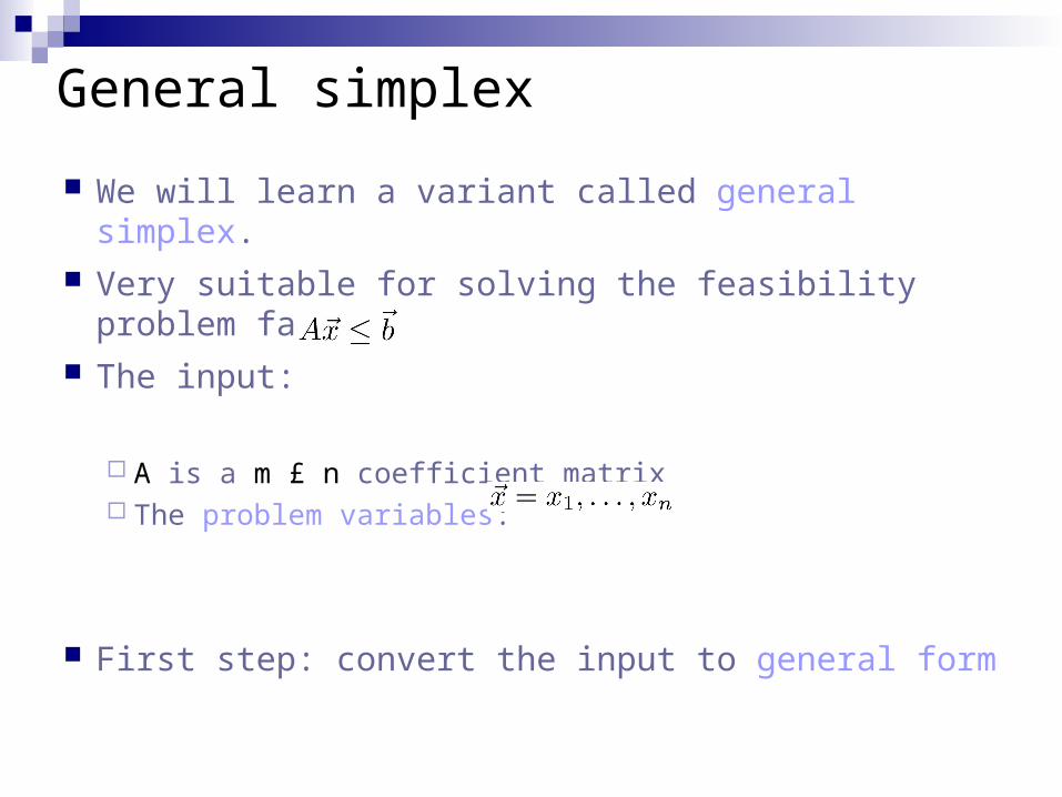
We will learn a variant called general simplex. Very suitable for solving the feasibility problem fast. The input:

A is a m £ n coefficient matrix The problem variables:

First step: convert the input to general form

General form

General form:

A combination of: Linear equalities of the form Lower and upper bounds on variables.

Converting to General Form

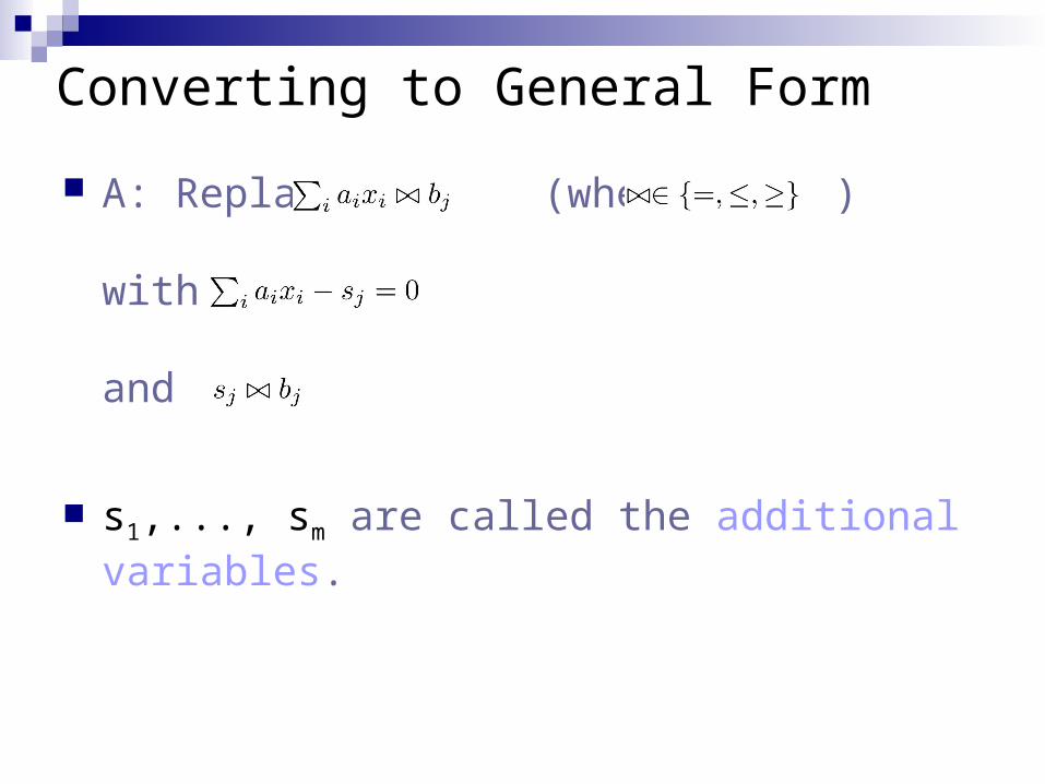
A: Replace (where )

with

and

s1,..., sm are called the additional variables.

Example 1

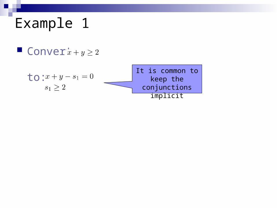
Convert

to: It is common to keep

the conjunctions implicit

Example 2

Convert

to:

Simplex basics…

Linear inequality constraints, geometrically, define a convex polyhedron.

© Wikipedia

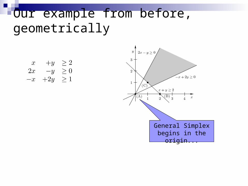
Our example from before, geometrically

General Simplex begins in the origin...

Matrix form

x y s1 s2 s3

Recall the general form: Due to the additional variables:

now A is an m £ (n + m) matrix.

The tableau

The diagonal part is inherent to the general form

We can instead write:

x y s1 s2 s3

x y

s1

s2

s3

This is called the tableau

The tableau

The tableau changes throughout the algorithm, but maintains its m £ n structure

Distinguish between basic and nonbasic variables Initially, basic variables = the additional variables.

x y

s1

s2

s3

Basic variables

Nonbasic variables

The tableau

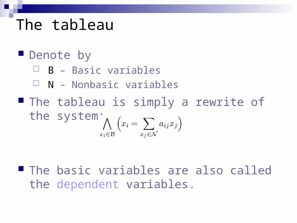
Denote by B – Basic variables N – Nonbasic variables

The tableau is simply a rewrite of the system:

The basic variables are also called the dependent variables.

The general simplex algorithm

Simplex maintains: The tableau, an assignment ® to all variables The bounds

Initially, B = additional variables N = problem variables ®(xi) = 0 for i 2 {1,...,n+m}

Invariants

Two invariants are maintained throughout:

1.

2. All nonbasic variables satisfy their bounds

Can you see why these invariants are maintained initially ?

We should check that they are indeed maintained

The general simplex algorithm

The initial assignment satisfies If the bounds of all basic variables are satisfied by ®,

return `Satisfiable’.

Otherwise... pivot.

Pivoting

Find a basic variable xi that violates its bounds.

Suppose that ®(xi) < li

Find a nonbasic variable xj such that aij > 0 and (xj) < uj, or

aij < 0 and (xj) > lj

Why ?

Pivoting

Find a basic variable xi that violates its bounds.

Suppose that ®(xi) < li

Find a nonbasic variable xj such that aij > 0 and (xj) < uj, or

aij < 0 and (xj) > lj

Such a variable xj is called suitable.

If there is no suitable variable – return ‘Unsatisfiable’ Why ?

Pivoting xi with xj

Solve equation i for xj:

From:

To:

Swap xi and xj, and update the i-th row accordingly.

From

To:

ai1 ... aij ... ain

-ai1

aij

... 1

aij

... -ain

aij

Pivoting xi with xj

Update all other rows: Replace xj with its equivalent obtained from row i:

Pivoting

Update ® as follows:

Increase ®(xj) by Now xj is a basic variable: it can violate its bounds.

Update ®(xi) accordingly

Q: What is now ®(xi) ?

Update for all other basic (dependent) variables.

Example

Recall the tableau and constraints in our example:

Initially assigns 0 to all variables

Bounds of s1 and s3 are violated

Example

Recall the tableau and constraints in our example:

We will solve s1

x is a suitable nonbasic variable for pivoting It has no upper bound

So now we pivot s1 with x

Example

Recall the tableau and constraints in our example:

Solve 1st row for x:

Replace x with s1 in other rows:

Example

The new state:

Solve 1st row for x:

Replace x with s1 in other rows:

Example

The new state:

What about the assignment ? We should increase x by

Hence, (x) = 0 + 2 = 2

Now s1 is equal to its lower bound: (s1) = 2

Update all the others

Example

The new state:

Now s3 violates its lower bound

Which nonbasic variable is suitable for pivoting ? That’s right… y

Example

The new state:

We should increase y by

Example

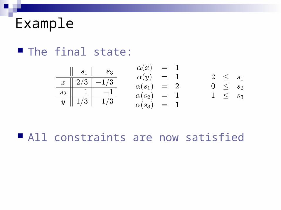
The final state:

All constraints are now satisfied

Observations

The additional variables: Only additional variables have bounds. These bounds are permanent. Additional variables exit the base only on extreme points

(their lower or upper bounds). When entering the base, they shift towards the other bound

and possibly cross it (violate it).

Observations

Can it be that we pivot(xi,xj) and then pivot(xj,xi) and enter a (local) cycle ? No. For example, suppose that aij > 0.

We increased (xj) so now (xi) = li.

After pivoting, possibly (xj) > uj

But aij’ = 1 / aij > 0, hence xi is not suitable.

Observations

Is termination guaranteed ? Not obvious.

Perhaps there are bigger cycles.

In order to avoid circles, we use Bland’s rule: determine a total order on the variables. Choose the first basic variable that violates its bounds, and

first nonbasic suitable variable for pivoting. It can be proven that this guarantees that no base is

repeated, which implies termination.

General-Simplex with Bland’s rule