daniel j. bernstein with big galois groups. computational ... · pdf file2013.07 talk slide...
TRANSCRIPT

Computational
algebraic number theory
tackles lattice-based cryptography
Daniel J. Bernstein
University of Illinois at Chicago &
Technische Universiteit Eindhoven
Moving to the left
Moving to the right
Big generator
Moving through the night
—Yes, “Big Generator”, 1987
2013.07 talk slide online:
“I think NTRU should switch to
random prime-degree extensions
with big Galois groups.”
2014.02 blog post:
“Here’s a concrete suggestion,
which I’ll call NTRU Prime,
for eliminating the structures
that I find worrisome in
existing ideal-lattice-based
encryption systems.”
NTRU Prime uses primes p; q
with field (Z=q)[x ]=(xp − x − 1).
Clear advantage of the usual
cyclotomics: minor speedup.
Extra advantage often claimed:
some “security reductions”.
But is this really an advantage?
Lange and I conjecture that
security is negatively correlated
with strength of reductions.
Disadvantage of cyclotomics:
many more symmetries
feed a scary attack strategy.
Already serious damage
to some lattice-based systems,
concerns about other systems.
Typical lattice advertisement:
“Because finding short vectors
in high-dimensional lattices
has been a notoriously hard
algorithmic question for hundreds
of years : : : we have solid and
unique evidence that lattice-based
cryptoschemes are secure.”
No. Dangerous exaggeration!
There are many obvious gaps
between lattice-based systems
and the classic lattice problems:
e.g., the systems use ideals.
Important to study these gaps.
2009 Smart–Vercauteren “Fully
homomorphic encryption with
relatively small key and ciphertext
sizes”: “Recovering the private
key given the public key is
therefore an instance of the small
principal ideal problem: : : : Given
a principal ideal : : : compute a
‘small’ generator of the ideal.
This is one of the core problems
in computational number theory
and has formed the basis of
previous cryptographic proposals,
see for example [3].”
Smart–Vercauteren, continued:
“There are currently two
approaches to the problem. : : :
In conclusion determining the
private key given only the public
key is an instance of a classical
and well studied problem in
algorithmic number theory. In
particular there are no efficient
solutions for this problem, and
the only sub-exponential method
does not find a solution which is
equivalent to our private key.”
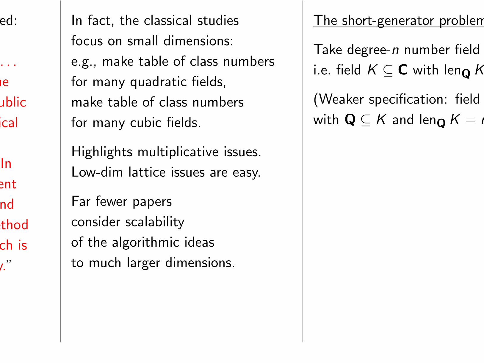
In fact, the classical studies
focus on small dimensions:
e.g., make table of class numbers
for many quadratic fields,
make table of class numbers
for many cubic fields.
Highlights multiplicative issues.
Low-dim lattice issues are easy.
Far fewer papers
consider scalability
of the algorithmic ideas
to much larger dimensions.

2009 Smart–Vercauteren “Fully
homomorphic encryption with
relatively small key and ciphertext
sizes”: “Recovering the private
key given the public key is
therefore an instance of the small
principal ideal problem: : : : Given
a principal ideal : : : compute a
‘small’ generator of the ideal.
This is one of the core problems
in computational number theory
and has formed the basis of
previous cryptographic proposals,
see for example [3].”
Smart–Vercauteren, continued:
“There are currently two
approaches to the problem. : : :
In conclusion determining the
private key given only the public
key is an instance of a classical
and well studied problem in
algorithmic number theory. In
particular there are no efficient
solutions for this problem, and
the only sub-exponential method
does not find a solution which is
equivalent to our private key.”
In fact, the classical studies
focus on small dimensions:
e.g., make table of class numbers
for many quadratic fields,
make table of class numbers
for many cubic fields.
Highlights multiplicative issues.
Low-dim lattice issues are easy.
Far fewer papers
consider scalability
of the algorithmic ideas
to much larger dimensions.
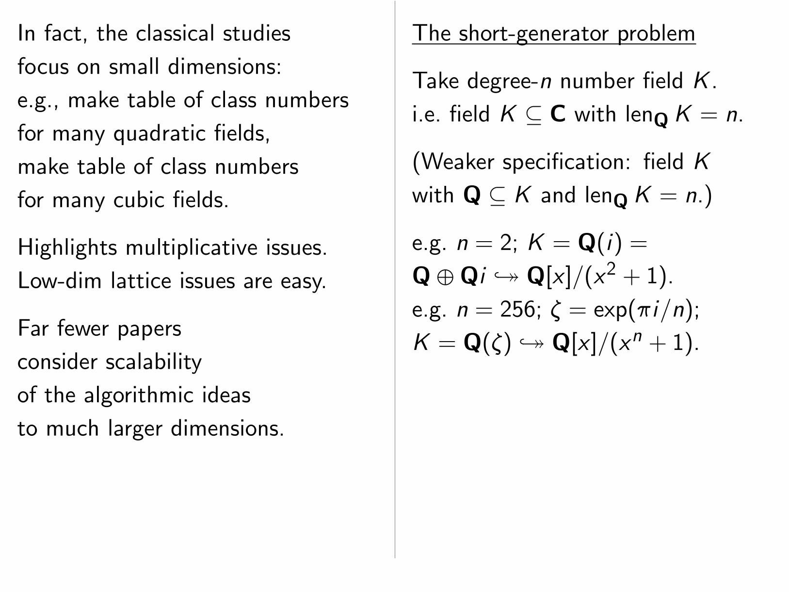
The short-generator problem
Take degree-n number field K.
i.e. field K ⊆ C with lenQK = n.
(Weaker specification: field K
with Q ⊆ K and lenQK = n.)

Smart–Vercauteren, continued:
“There are currently two
approaches to the problem. : : :
In conclusion determining the
private key given only the public
key is an instance of a classical
and well studied problem in
algorithmic number theory. In
particular there are no efficient
solutions for this problem, and
the only sub-exponential method
does not find a solution which is
equivalent to our private key.”
In fact, the classical studies
focus on small dimensions:
e.g., make table of class numbers
for many quadratic fields,
make table of class numbers
for many cubic fields.
Highlights multiplicative issues.
Low-dim lattice issues are easy.
Far fewer papers
consider scalability
of the algorithmic ideas
to much larger dimensions.
The short-generator problem
Take degree-n number field K.
i.e. field K ⊆ C with lenQK = n.
(Weaker specification: field K
with Q ⊆ K and lenQK = n.)
e.g. n = 2; K = Q(i) =
Q⊕Qi ,� Q[x ]=(x2 + 1).
e.g. n = 256; “ = exp(ıi=n);
K = Q(“) ,� Q[x ]=(xn + 1).
e.g. n = 660; “ = exp(2ıi=661);
K = Q(“) ,� Q[x ]=(xn + · · ·+ 1).
e.g. K=Q(√
2;√
3;√
5; : : : ;√
29).
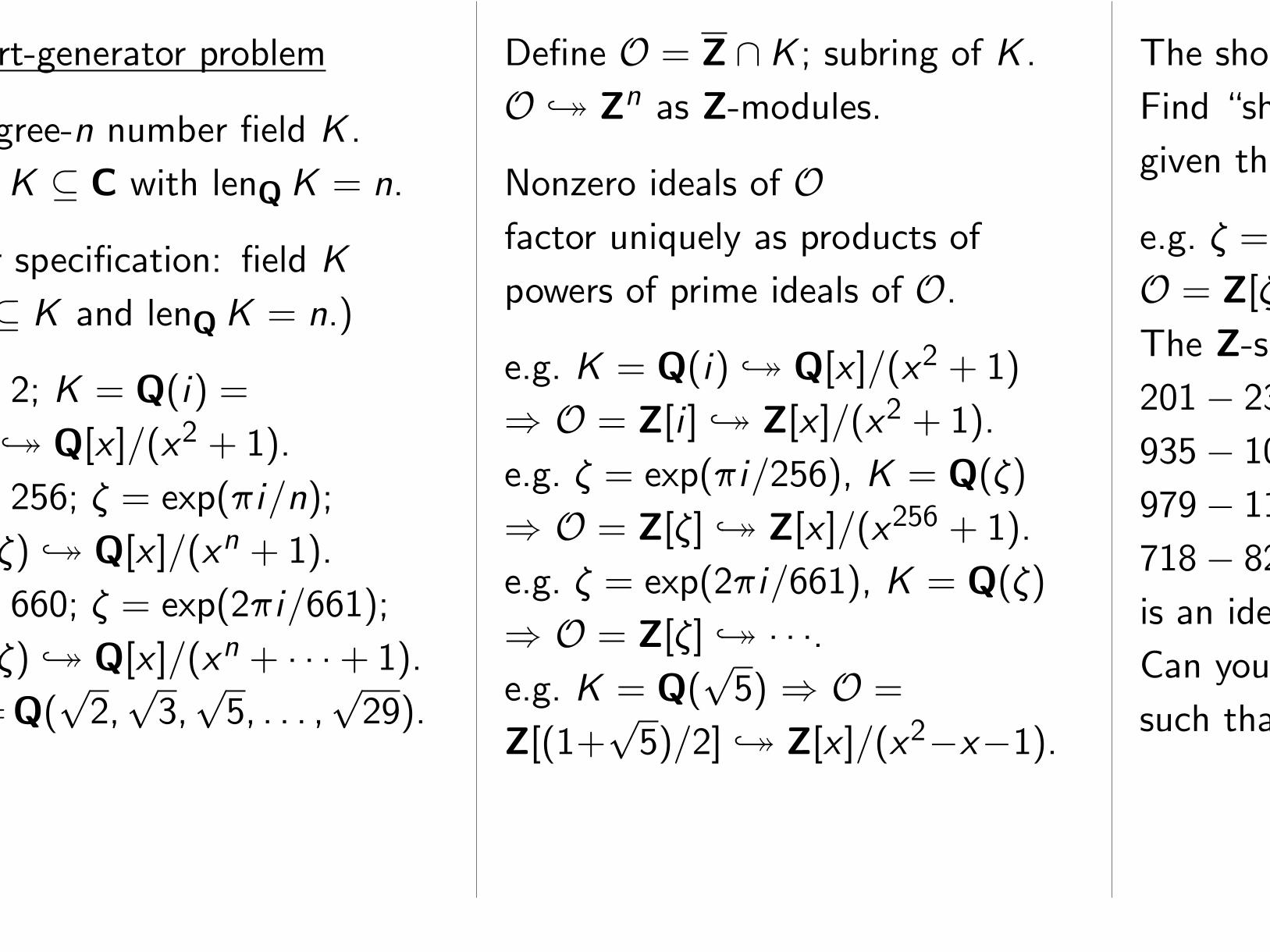
Define O = Z ∩K; subring of K.
O ,� Zn as Z-modules.
Nonzero ideals of Ofactor uniquely as products of
powers of prime ideals of O.

In fact, the classical studies
focus on small dimensions:
e.g., make table of class numbers
for many quadratic fields,
make table of class numbers
for many cubic fields.
Highlights multiplicative issues.
Low-dim lattice issues are easy.
Far fewer papers
consider scalability
of the algorithmic ideas
to much larger dimensions.
The short-generator problem
Take degree-n number field K.
i.e. field K ⊆ C with lenQK = n.
(Weaker specification: field K
with Q ⊆ K and lenQK = n.)
e.g. n = 2; K = Q(i) =
Q⊕Qi ,� Q[x ]=(x2 + 1).
e.g. n = 256; “ = exp(ıi=n);
K = Q(“) ,� Q[x ]=(xn + 1).
e.g. n = 660; “ = exp(2ıi=661);
K = Q(“) ,� Q[x ]=(xn + · · ·+ 1).
e.g. K=Q(√
2;√
3;√
5; : : : ;√
29).
Define O = Z ∩K; subring of K.
O ,� Zn as Z-modules.
Nonzero ideals of Ofactor uniquely as products of
powers of prime ideals of O.
e.g. K = Q(i) ,� Q[x ]=(x2 + 1)
⇒ O = Z[i ] ,� Z[x ]=(x2 + 1).
e.g. “ = exp(ıi=256), K = Q(“)
⇒ O = Z[“] ,� Z[x ]=(x256 + 1).
e.g. “ = exp(2ıi=661), K = Q(“)
⇒ O = Z[“] ,� · · ·.

The short-generator problem
Take degree-n number field K.
i.e. field K ⊆ C with lenQK = n.
(Weaker specification: field K
with Q ⊆ K and lenQK = n.)
e.g. n = 2; K = Q(i) =
Q⊕Qi ,� Q[x ]=(x2 + 1).
e.g. n = 256; “ = exp(ıi=n);
K = Q(“) ,� Q[x ]=(xn + 1).
e.g. n = 660; “ = exp(2ıi=661);
K = Q(“) ,� Q[x ]=(xn + · · ·+ 1).
e.g. K=Q(√
2;√
3;√
5; : : : ;√
29).
Define O = Z ∩K; subring of K.
O ,� Zn as Z-modules.
Nonzero ideals of Ofactor uniquely as products of
powers of prime ideals of O.
e.g. K = Q(i) ,� Q[x ]=(x2 + 1)
⇒ O = Z[i ] ,� Z[x ]=(x2 + 1).
e.g. “ = exp(ıi=256), K = Q(“)
⇒ O = Z[“] ,� Z[x ]=(x256 + 1).
e.g. “ = exp(2ıi=661), K = Q(“)
⇒ O = Z[“] ,� · · ·.e.g. K = Q(
√5) ⇒ O =
Z[(1+√
5)=2] ,� Z[x ]=(x2−x−1).
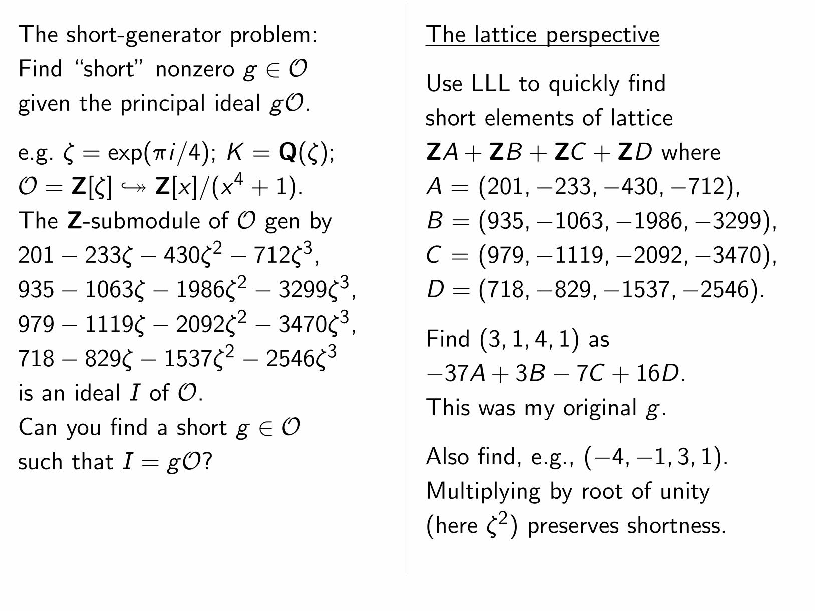
The short-generator problem:
Find “short” nonzero g ∈ Ogiven the principal ideal gO.
e.g. “ = exp(ıi=4); K = Q(“);
O = Z[“] ,� Z[x ]=(x4 + 1).
The Z-submodule of O gen by
201− 233“ − 430“2 − 712“3,
935− 1063“ − 1986“2 − 3299“3,
979− 1119“ − 2092“2 − 3470“3,
718− 829“ − 1537“2 − 2546“3
is an ideal I of O.
Can you find a short g ∈ Osuch that I = gO?

The short-generator problem
Take degree-n number field K.
i.e. field K ⊆ C with lenQK = n.
(Weaker specification: field K
with Q ⊆ K and lenQK = n.)
e.g. n = 2; K = Q(i) =
Q⊕Qi ,� Q[x ]=(x2 + 1).
e.g. n = 256; “ = exp(ıi=n);
K = Q(“) ,� Q[x ]=(xn + 1).
e.g. n = 660; “ = exp(2ıi=661);
K = Q(“) ,� Q[x ]=(xn + · · ·+ 1).
e.g. K=Q(√
2;√
3;√
5; : : : ;√
29).
Define O = Z ∩K; subring of K.
O ,� Zn as Z-modules.
Nonzero ideals of Ofactor uniquely as products of
powers of prime ideals of O.
e.g. K = Q(i) ,� Q[x ]=(x2 + 1)
⇒ O = Z[i ] ,� Z[x ]=(x2 + 1).
e.g. “ = exp(ıi=256), K = Q(“)
⇒ O = Z[“] ,� Z[x ]=(x256 + 1).
e.g. “ = exp(2ıi=661), K = Q(“)
⇒ O = Z[“] ,� · · ·.e.g. K = Q(
√5) ⇒ O =
Z[(1+√
5)=2] ,� Z[x ]=(x2−x−1).
The short-generator problem:
Find “short” nonzero g ∈ Ogiven the principal ideal gO.
e.g. “ = exp(ıi=4); K = Q(“);
O = Z[“] ,� Z[x ]=(x4 + 1).
The Z-submodule of O gen by
201− 233“ − 430“2 − 712“3,
935− 1063“ − 1986“2 − 3299“3,
979− 1119“ − 2092“2 − 3470“3,
718− 829“ − 1537“2 − 2546“3
is an ideal I of O.
Can you find a short g ∈ Osuch that I = gO?
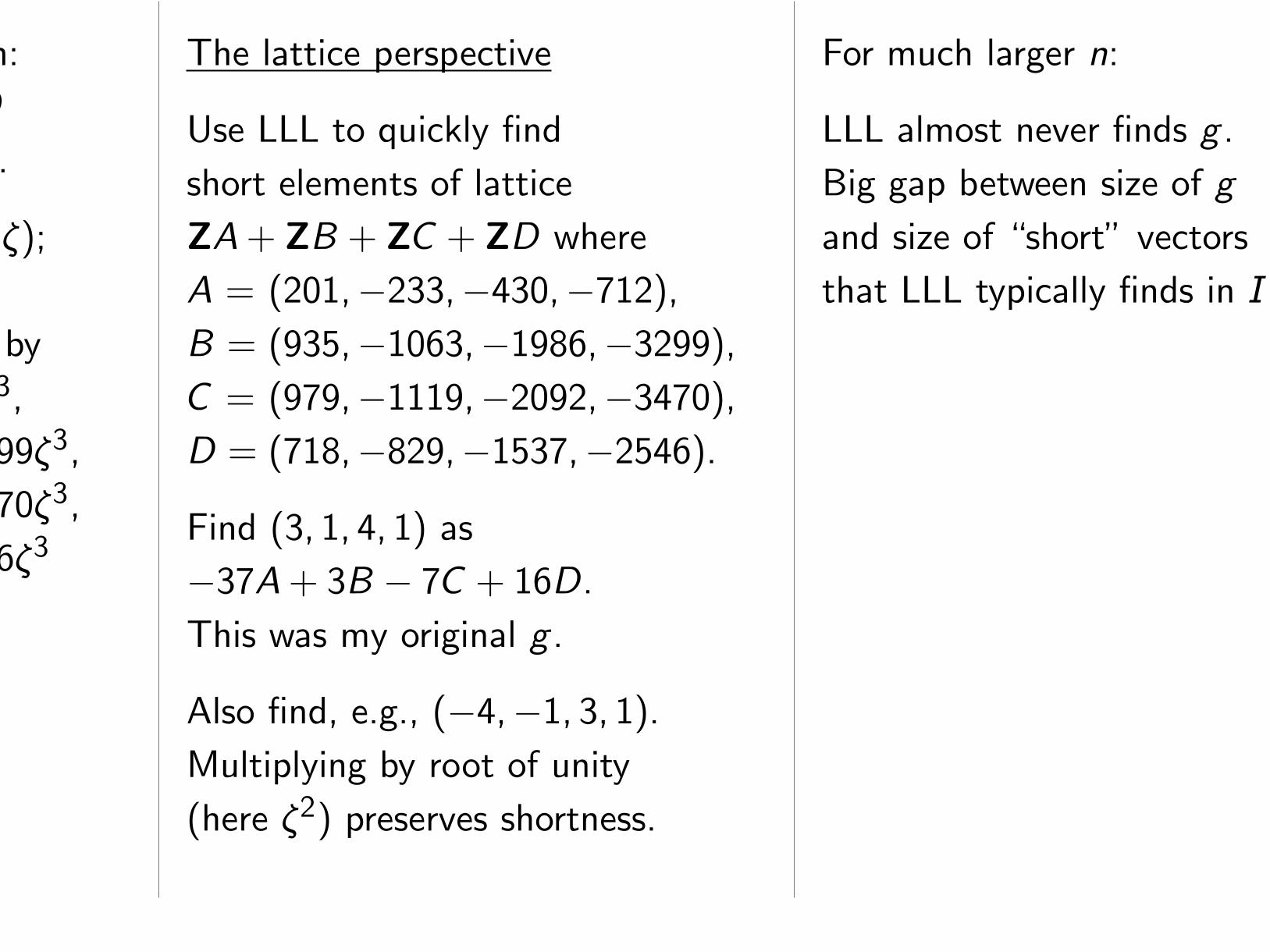
The lattice perspective
Use LLL to quickly find
short elements of lattice
ZA+ ZB + ZC + ZD where
A = (201;−233;−430;−712);
B = (935;−1063;−1986;−3299);
C = (979;−1119;−2092;−3470);
D = (718;−829;−1537;−2546):

Define O = Z ∩K; subring of K.
O ,� Zn as Z-modules.
Nonzero ideals of Ofactor uniquely as products of
powers of prime ideals of O.
e.g. K = Q(i) ,� Q[x ]=(x2 + 1)
⇒ O = Z[i ] ,� Z[x ]=(x2 + 1).
e.g. “ = exp(ıi=256), K = Q(“)
⇒ O = Z[“] ,� Z[x ]=(x256 + 1).
e.g. “ = exp(2ıi=661), K = Q(“)
⇒ O = Z[“] ,� · · ·.e.g. K = Q(
√5) ⇒ O =
Z[(1+√
5)=2] ,� Z[x ]=(x2−x−1).
The short-generator problem:
Find “short” nonzero g ∈ Ogiven the principal ideal gO.
e.g. “ = exp(ıi=4); K = Q(“);
O = Z[“] ,� Z[x ]=(x4 + 1).
The Z-submodule of O gen by
201− 233“ − 430“2 − 712“3,
935− 1063“ − 1986“2 − 3299“3,
979− 1119“ − 2092“2 − 3470“3,
718− 829“ − 1537“2 − 2546“3
is an ideal I of O.
Can you find a short g ∈ Osuch that I = gO?
The lattice perspective
Use LLL to quickly find
short elements of lattice
ZA+ ZB + ZC + ZD where
A = (201;−233;−430;−712);
B = (935;−1063;−1986;−3299);
C = (979;−1119;−2092;−3470);
D = (718;−829;−1537;−2546):
Find (3; 1; 4; 1) as
−37A+ 3B − 7C + 16D.
This was my original g .
Also find, e.g., (−4;−1; 3; 1).
Multiplying by root of unity
(here “2) preserves shortness.
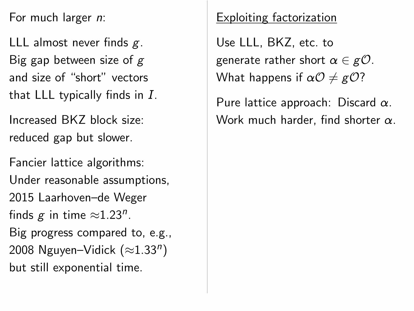
For much larger n:
LLL almost never finds g .
Big gap between size of g
and size of “short” vectors
that LLL typically finds in I.

The short-generator problem:
Find “short” nonzero g ∈ Ogiven the principal ideal gO.
e.g. “ = exp(ıi=4); K = Q(“);
O = Z[“] ,� Z[x ]=(x4 + 1).
The Z-submodule of O gen by
201− 233“ − 430“2 − 712“3,
935− 1063“ − 1986“2 − 3299“3,
979− 1119“ − 2092“2 − 3470“3,
718− 829“ − 1537“2 − 2546“3
is an ideal I of O.
Can you find a short g ∈ Osuch that I = gO?
The lattice perspective
Use LLL to quickly find
short elements of lattice
ZA+ ZB + ZC + ZD where
A = (201;−233;−430;−712);
B = (935;−1063;−1986;−3299);
C = (979;−1119;−2092;−3470);
D = (718;−829;−1537;−2546):
Find (3; 1; 4; 1) as
−37A+ 3B − 7C + 16D.
This was my original g .
Also find, e.g., (−4;−1; 3; 1).
Multiplying by root of unity
(here “2) preserves shortness.
For much larger n:
LLL almost never finds g .
Big gap between size of g
and size of “short” vectors
that LLL typically finds in I.
Increased BKZ block size:
reduced gap but slower.
Fancier lattice algorithms:
Under reasonable assumptions,
2015 Laarhoven–de Weger
finds g in time ≈1:23n.
Big progress compared to, e.g.,
2008 Nguyen–Vidick (≈1:33n)
but still exponential time.
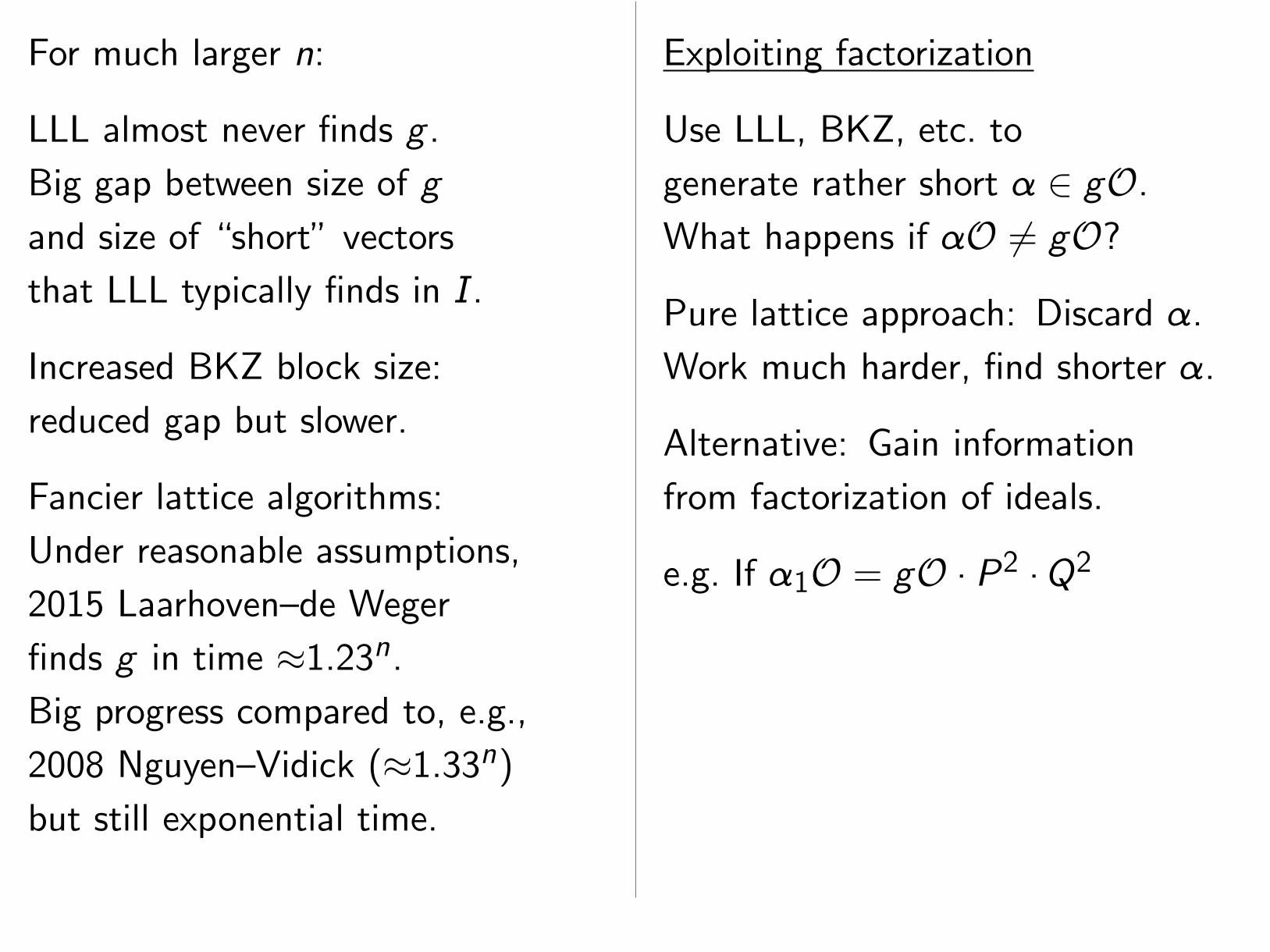
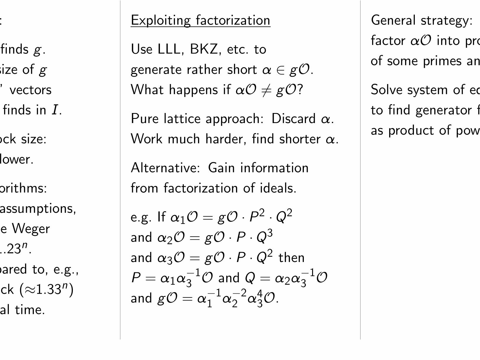
Exploiting factorization
Use LLL, BKZ, etc. to
generate rather short ¸ ∈ gO.
What happens if ¸O 6= gO?
Pure lattice approach: Discard ¸.
Work much harder, find shorter ¸.

The lattice perspective
Use LLL to quickly find
short elements of lattice
ZA+ ZB + ZC + ZD where
A = (201;−233;−430;−712);
B = (935;−1063;−1986;−3299);
C = (979;−1119;−2092;−3470);
D = (718;−829;−1537;−2546):
Find (3; 1; 4; 1) as
−37A+ 3B − 7C + 16D.
This was my original g .
Also find, e.g., (−4;−1; 3; 1).
Multiplying by root of unity
(here “2) preserves shortness.
For much larger n:
LLL almost never finds g .
Big gap between size of g
and size of “short” vectors
that LLL typically finds in I.
Increased BKZ block size:
reduced gap but slower.
Fancier lattice algorithms:
Under reasonable assumptions,
2015 Laarhoven–de Weger
finds g in time ≈1:23n.
Big progress compared to, e.g.,
2008 Nguyen–Vidick (≈1:33n)
but still exponential time.
Exploiting factorization
Use LLL, BKZ, etc. to
generate rather short ¸ ∈ gO.
What happens if ¸O 6= gO?
Pure lattice approach: Discard ¸.
Work much harder, find shorter ¸.
Alternative: Gain information
from factorization of ideals.
e.g. If ¸1O = gO · P 2 · Q2
and ¸2O = gO · P · Q3
and ¸3O = gO · P · Q2

For much larger n:
LLL almost never finds g .
Big gap between size of g
and size of “short” vectors
that LLL typically finds in I.
Increased BKZ block size:
reduced gap but slower.
Fancier lattice algorithms:
Under reasonable assumptions,
2015 Laarhoven–de Weger
finds g in time ≈1:23n.
Big progress compared to, e.g.,
2008 Nguyen–Vidick (≈1:33n)
but still exponential time.
Exploiting factorization
Use LLL, BKZ, etc. to
generate rather short ¸ ∈ gO.
What happens if ¸O 6= gO?
Pure lattice approach: Discard ¸.
Work much harder, find shorter ¸.
Alternative: Gain information
from factorization of ideals.
e.g. If ¸1O = gO · P 2 · Q2
and ¸2O = gO · P · Q3
and ¸3O = gO · P · Q2 then
P = ¸1¸−13 O and Q = ¸2¸
−13 O
and gO = ¸−11 ¸−2
2 ¸43O.
General strategy: For many ¸’s,
factor ¸O into products of powers
of some primes and gO.
Solve system of equations
to find generator for gOas product of powers of the ¸’s.
For much larger n:
LLL almost never finds g .
Big gap between size of g
and size of “short” vectors
that LLL typically finds in I.
Increased BKZ block size:
reduced gap but slower.
Fancier lattice algorithms:
Under reasonable assumptions,
2015 Laarhoven–de Weger
finds g in time ≈1:23n.
Big progress compared to, e.g.,
2008 Nguyen–Vidick (≈1:33n)
but still exponential time.
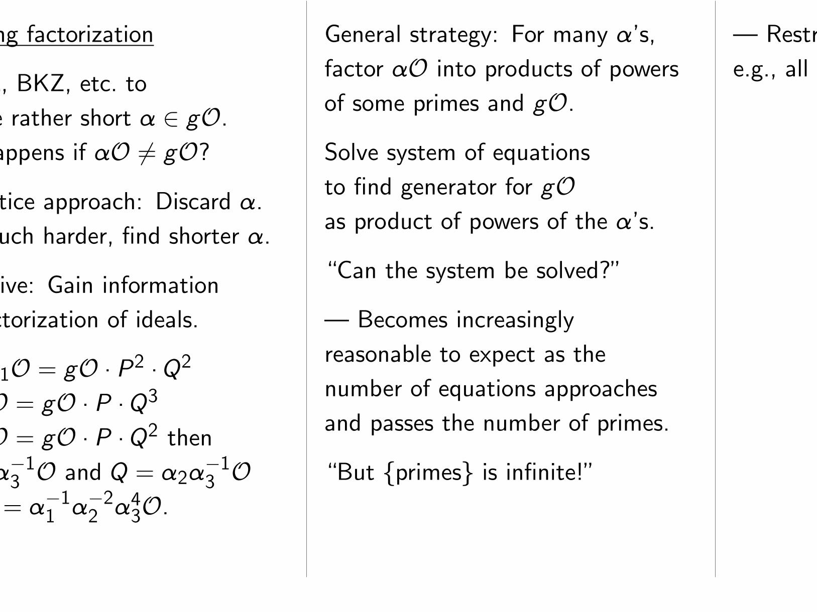
Exploiting factorization
Use LLL, BKZ, etc. to
generate rather short ¸ ∈ gO.
What happens if ¸O 6= gO?
Pure lattice approach: Discard ¸.
Work much harder, find shorter ¸.
Alternative: Gain information
from factorization of ideals.
e.g. If ¸1O = gO · P 2 · Q2
and ¸2O = gO · P · Q3
and ¸3O = gO · P · Q2 then
P = ¸1¸−13 O and Q = ¸2¸
−13 O
and gO = ¸−11 ¸−2
2 ¸43O.
General strategy: For many ¸’s,
factor ¸O into products of powers
of some primes and gO.
Solve system of equations
to find generator for gOas product of powers of the ¸’s.

For much larger n:
LLL almost never finds g .
Big gap between size of g
and size of “short” vectors
that LLL typically finds in I.
Increased BKZ block size:
reduced gap but slower.
Fancier lattice algorithms:
Under reasonable assumptions,
2015 Laarhoven–de Weger
finds g in time ≈1:23n.
Big progress compared to, e.g.,
2008 Nguyen–Vidick (≈1:33n)
but still exponential time.
Exploiting factorization
Use LLL, BKZ, etc. to
generate rather short ¸ ∈ gO.
What happens if ¸O 6= gO?
Pure lattice approach: Discard ¸.
Work much harder, find shorter ¸.
Alternative: Gain information
from factorization of ideals.
e.g. If ¸1O = gO · P 2 · Q2
and ¸2O = gO · P · Q3
and ¸3O = gO · P · Q2 then
P = ¸1¸−13 O and Q = ¸2¸
−13 O
and gO = ¸−11 ¸−2
2 ¸43O.
General strategy: For many ¸’s,
factor ¸O into products of powers
of some primes and gO.
Solve system of equations
to find generator for gOas product of powers of the ¸’s.
“Can the system be solved?”
— Becomes increasingly
reasonable to expect as the
number of equations approaches
and passes the number of primes.
“But {primes} is infinite!”
— Restrict to a “factor base”:
e.g., all primes of norm ≤y .
“But what if ¸O doesn’t
factor into those primes?”
— Then throw it away.
But often it does factor.
Familiar issue from
“index calculus” DL methods,
CFRAC, LS, QS, NFS, etc.
Model the norm of (¸=g)Oas “random” integer in [1; x ];
y -smoothness chance ≈1=y
if log y ≈p
(1=2) log x log log x .
Variation: Ignore gO.
Generate rather short ¸ ∈ O,
factor ¸O into small primes.
After enough ¸’s,
solve system of equations;
obtain generator for each prime.
After this precomputation,
factor one ¸O ⊆ gO;
obtain generator for gO.
“Do all primes have generators?”
— Standard heuristics:
For many (most?) number fields,
yes; but for big cyclotomics, no!
Modulo a few small primes, yes.
{principal nonzero ideals} is
kernel of a semigroup map
{nonzero ideals}� C where
C is a finite abelian group,
the “class group of K”.
Fundamental object of study
in algebraic number theory.
Factoring many small ¸Ois a standard textbook method
of computing class group
and generators of ideals.
Also compute unit group O∗
via ratios of generators.
A note on time analysis
Smart–Vercauteren statement
regarding similar algorithm by
Buchmann: “This method has
complexity exp(O(N logN) ·plog(∆) · log log(∆)).”
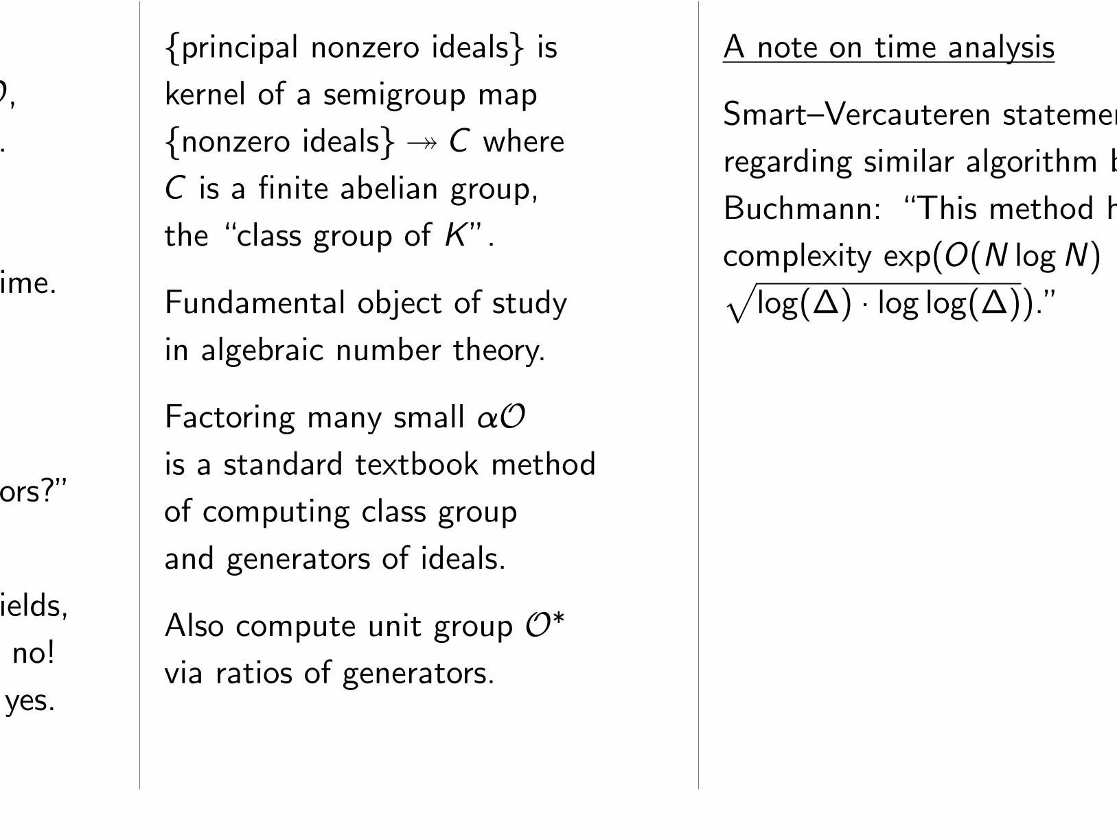
— [citation needed]
Did they mean Θ? And +?
exp(Θ(N logN)) factor
for short-vector enumeration?
Silly: BKZ works just fine.
The whole algorithm will be
subexponential unless norms are
much worse than exponential.
Big generator
Smart–Vercauteren: “However
this method is likely to produce
a generator of large height, i.e.,
with large coefficients. Indeed so
large, that writing the obtained
generator down as a polynomial in
„ may take exponential time.”
Indeed, generator found for gO is
product of powers of various ¸’s.
Must be gu for some u ∈ O∗,but extremely unlikely to be g .
How do we find g from gu?
There are exactly n distinct
ring maps ’1; : : : ; ’n : K → C.
Define Log : K∗ → Rn by
Log = (log |’1|; : : : ; log |’n|).
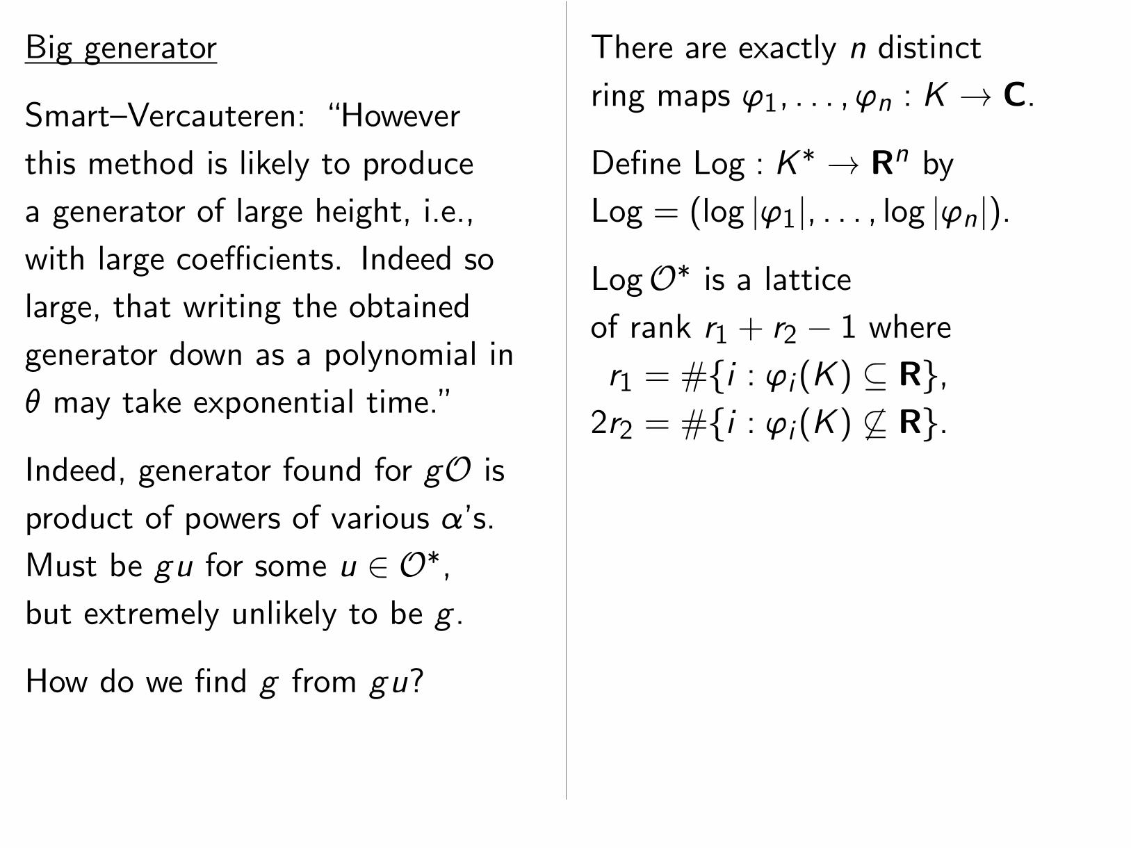
LogO∗ is a lattice
of rank r1 + r2 − 1 where
r1 = #{i : ’i (K) ⊆ R},2r2 = #{i : ’i (K) 6⊆ R}.
e.g. “ = exp(ıi=256), K = Q(“):
images of “ under ring maps
are “; “3; “5; : : : ; “511.
r1 = 0; r2 = 128; rank 127.
Compute Log gu
as sum of multiples of Log¸
for the original ¸’s.
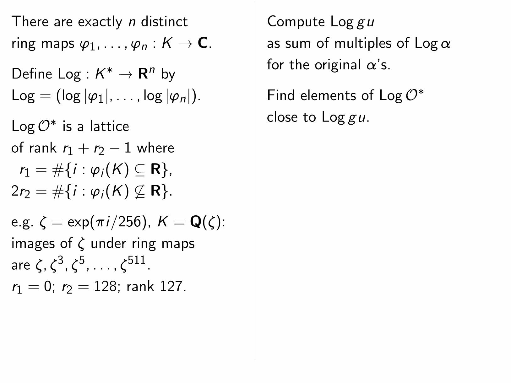
Find elements of LogO∗
close to Log gu.
This is a close-vector problem
(“bounded-distance decoding”).
“Embedding” heuristic:
CVP as fast as SVP.
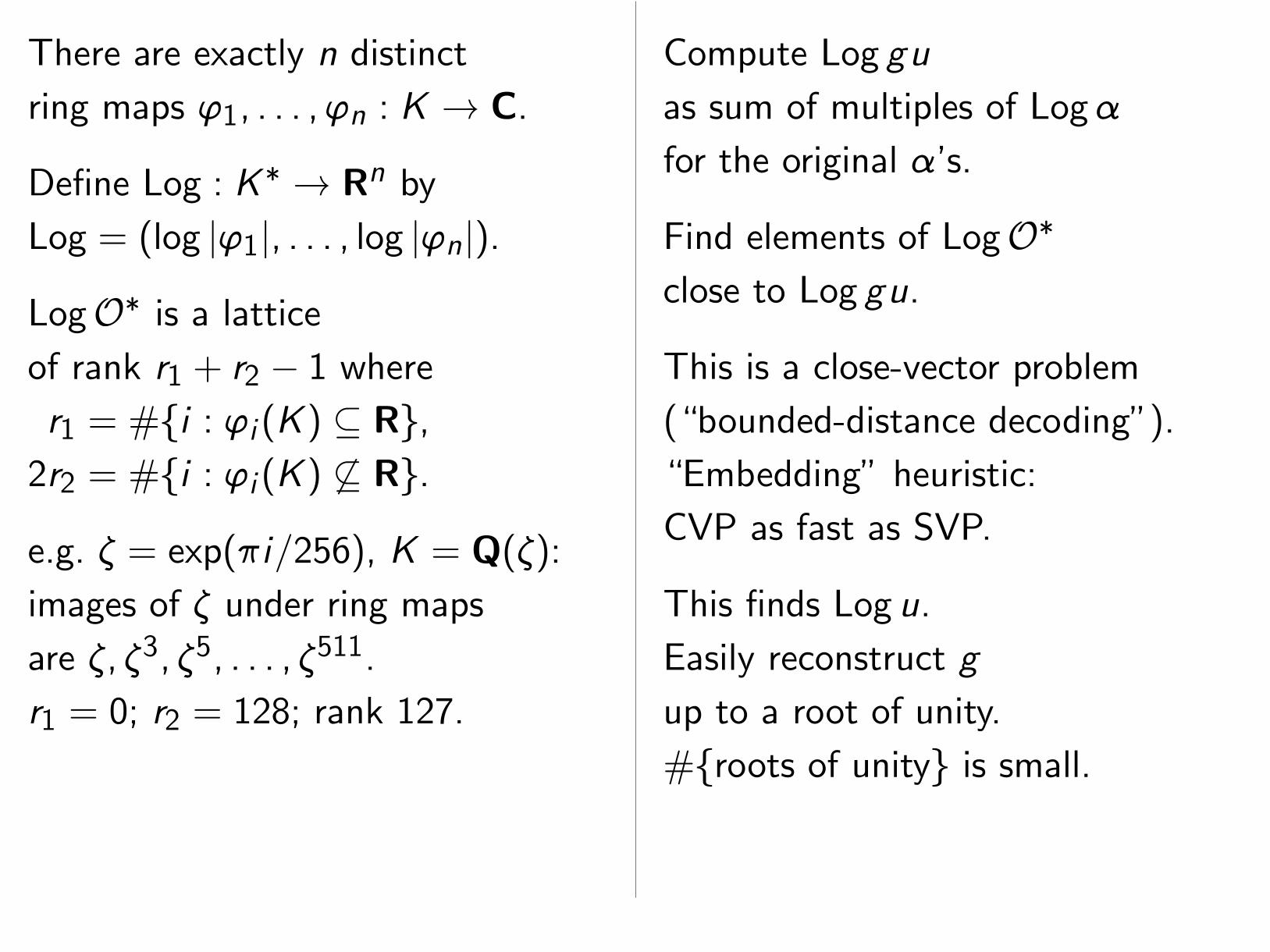
This finds Log u.
Easily reconstruct g
up to a root of unity.
#{roots of unity} is small.
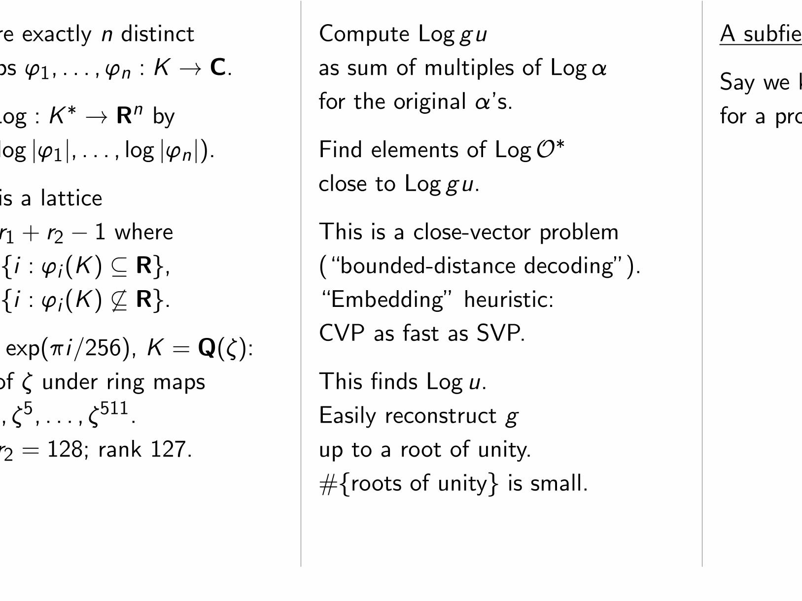
A subfield-logarithm attack
Say we know Log normK:F g
for a proper subfield F ⊂ K.
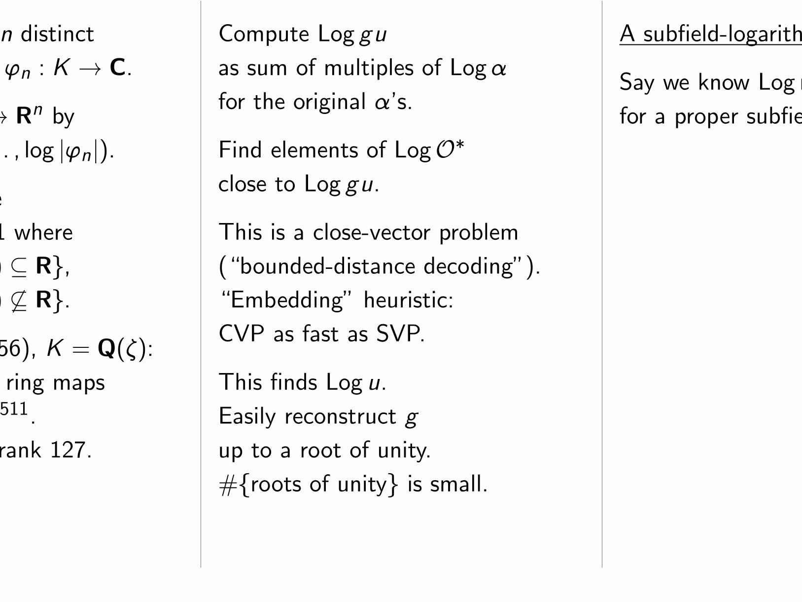
We also know Log normK:F gu,
so we know Log normK:F u.
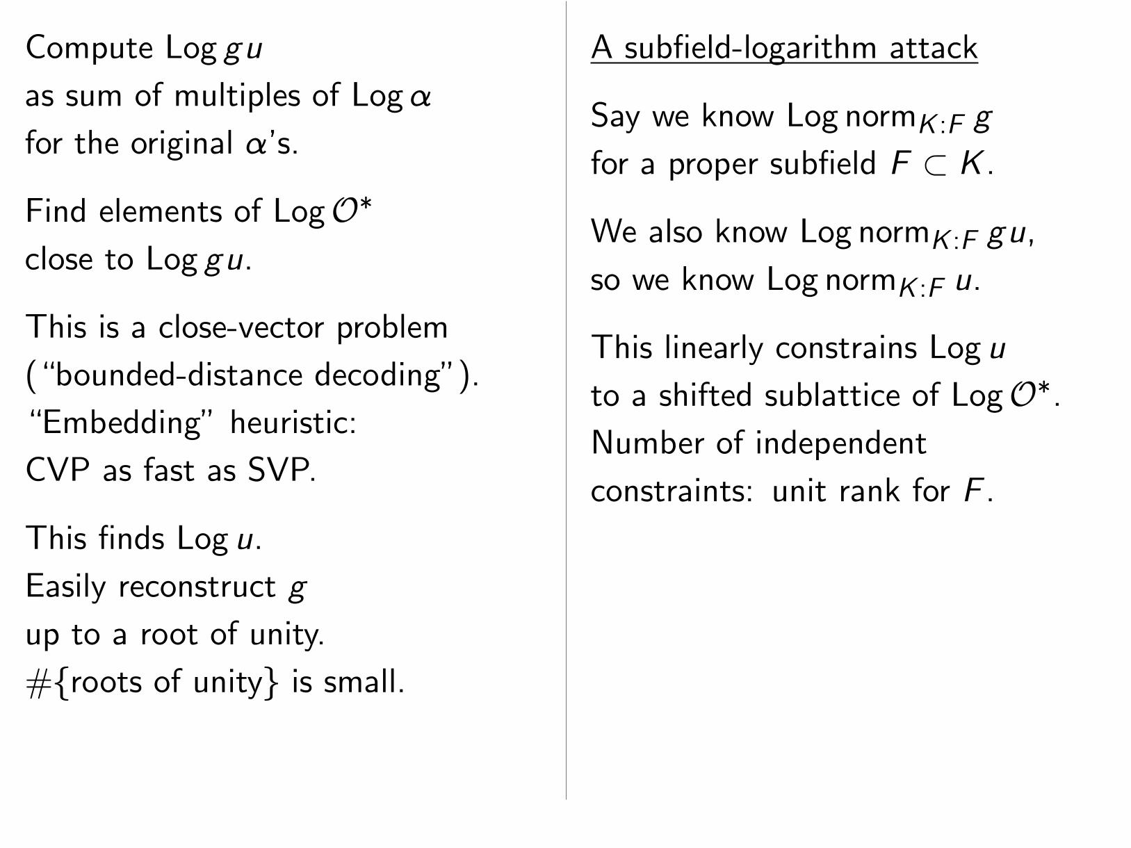
This linearly constrains Log u
to a shifted sublattice of LogO∗.Number of independent
constraints: unit rank for F .
Find elements close to Log gu.
Lower-dimension lattice problem,
if unit rank of F is positive.
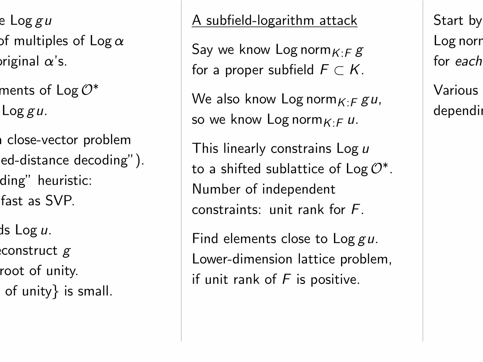
Start by recursively computing
Log normK:F g via norm of gOfor each F ⊂ K.
Various constraints on Log u,
depending on subfield structure.
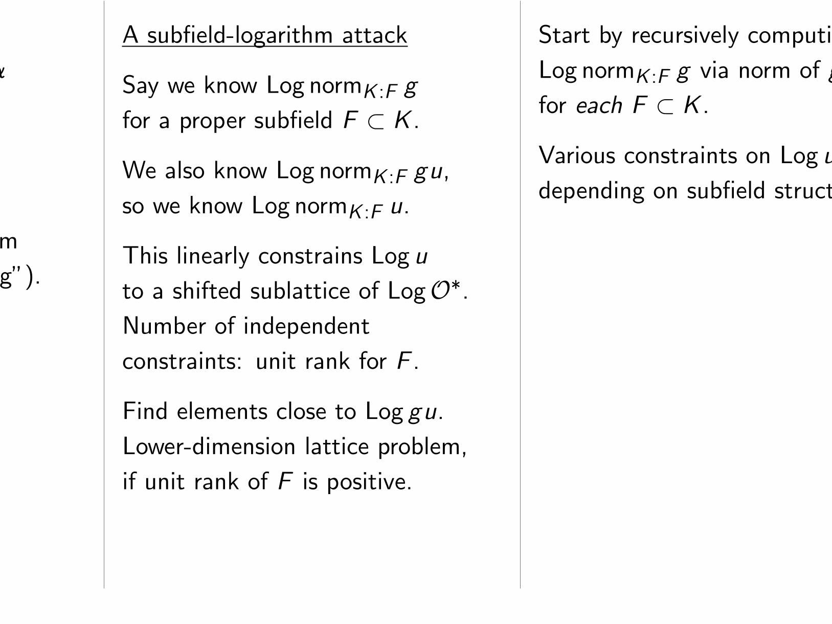
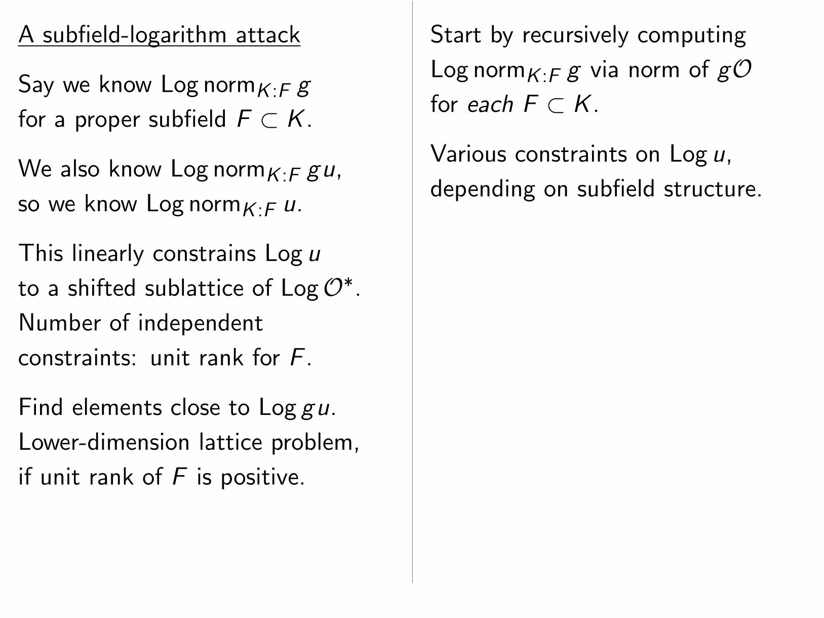
e.g. “ = exp(2ıi=661), K = Q(“).
Degrees of subfields of K:
660
330qqq
220��
132
22
60
MMM
165qqq
110�� qqq
66
22 qqq44
222 ��� 30
TTTTTTT ��20
TTTTTTT22
12
TTTTTTTMMMM
55zz
33
DD zz22
DD zz15
VVVVVVVVV zz10
VVVVVVVVV zz6
VVVVVVVVVVDDD zzz
4
VVVVVVVVVVDDD
11
MMMM 22 ��5
TTTTTTTT �� qqqq3
TTTTTTTT22 zzz
2
TTTTTTTT22 �� qqqqq
1
MMMM22 �� qqqqq
Most extreme case:
Composite of quadratics, such as
K=Q(√
2;√
3;√
5; : : : ;√
29).
CVP becomes trivial!
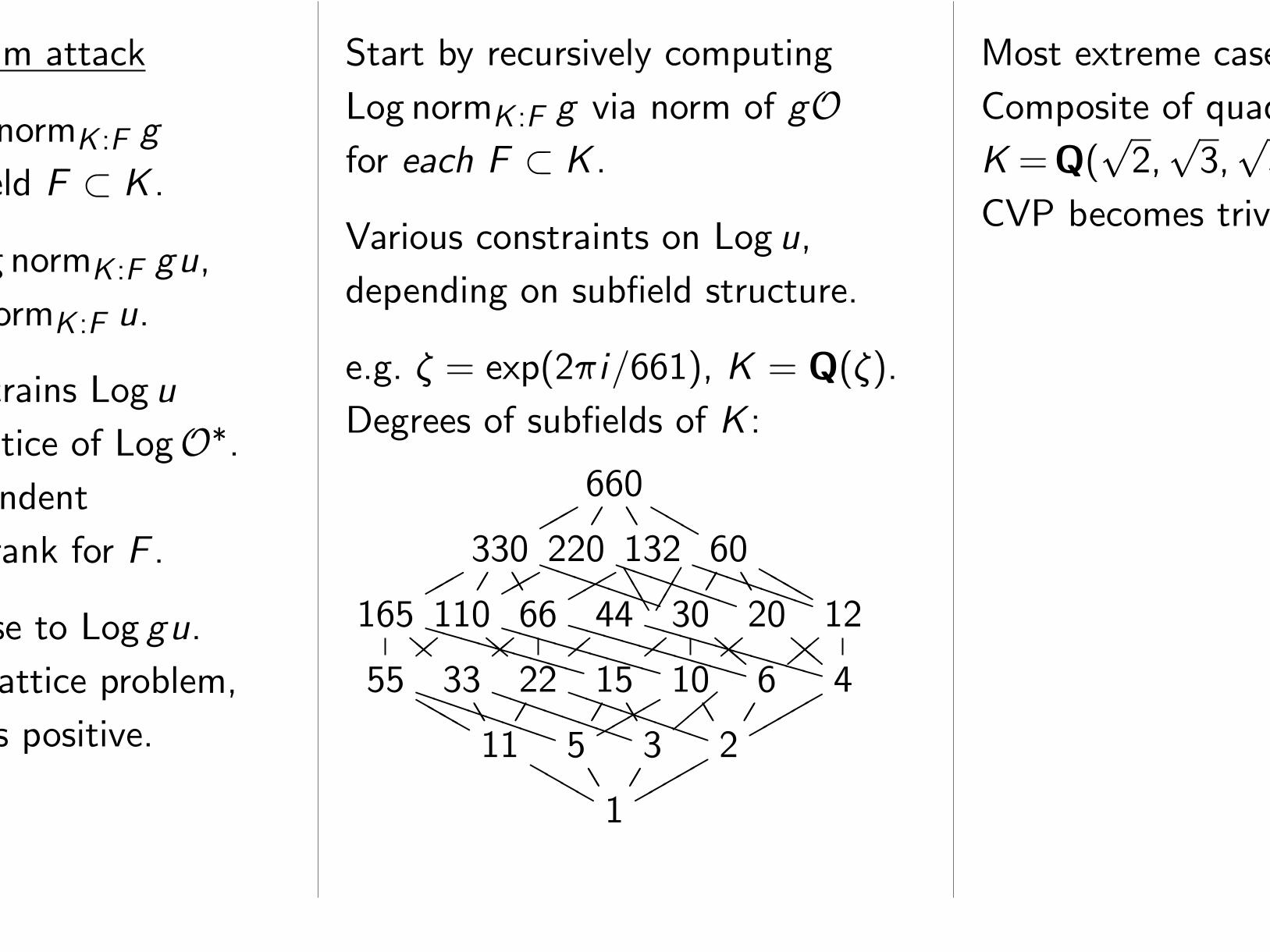
Many intermediate cases.
“Subexponential in cyclotomic
rings of highly smooth index”:
It’s much more general than that.
For cyclotomics this approach
is superseded by subsequent
Campbell–Groves–Shepherd
algorithm, using known (good)
basis for cyclotomic units.