damping models for structural vibrationengweb.swan.ac.uk/~adhikaris/fulltext/other/ftphd.pdf ·...
TRANSCRIPT

Damping Models for Structural Vibration
Cambridge UniversityEngineering Department
A dissertationsubmitted to the University of Cambridgefor the Degree of Doctor of Philosophy
by
Sondipon AdhikariTrinity College, Cambridge
September, 2000

ii

To my Parents

iv

Declaration
This dissertation describes part of the research performed at the Cambridge University EngineeringDepartment between October 1997 and September 2000. It is the result of my own work andincludes nothing which is the outcome of work done in collaboration, except where stated. Thedissertation contains approximately 63,000 words, 120 figures and 160 references.
Sondipon AdhikariSeptember, 2000
v

vi DECLARATION

Abstract
This dissertation reports a systematic study on analysis and identification of multiple parameter dampedmechanical systems. The attention is focused on viscously and non-viscously damped multiple degree-of-freedom linear vibrating systems. The non-viscous damping model is such that the damping forces dependon the past history of motion via convolution integrals over some kernel functions. The familiar viscousdamping model is a special case of this general linear damping model when the kernel functions have nomemory.
The concept of proportional damping is critically examined and a generalized form of proportionaldamping is proposed. It is shown that the proportional damping can exist even when the damping mechanismis non-viscous.
Classical modal analysis is extended to deal with general non-viscously damped multiple degree-of-freedom linear dynamic systems. The new method is similar to the existing method with some modificationsdue to non-viscous effect of the damping mechanism. The concept of (complex) elastic modes and non-viscous modes have been introduced and numerical methods are suggested to obtain them. It is furthershown that the system response can be obtained exactly in terms of these modes. Mode orthogonalityrelationships, known for undamped or viscously damped systems, have been generalized to non-viscouslydamped systems. Several useful results which relate the modes with the system matrices are developed.
These theoretical developments on non-viscously damped systems, in line with classical modal analy-sis, give impetus towards understanding damping mechanisms in general mechanical systems. Based on afirst-order perturbation method, an approach is suggested to the identify non-proportional viscous dampingmatrix from the measured complex modes and frequencies. This approach is then further extended to iden-tify non-viscous damping models. Both the approaches are simple, direct, and can be used with incompletemodal data.
It is observed that these methods yield non-physical results by breaking the symmetry of the fitteddamping matrix when the damping mechanism of the original system is significantly different from what isfitted. To solve this problem, approaches are suggested to preserve the symmetry of the identified viscousand non-viscous damping matrix.
The damping identification methods are applied experimentally to a beam in bending vibration withlocalized constrained layer damping. Since the identification method requires complex modal data, a gen-eral method for identification of complex modes and complex frequencies from a set of measured transferfunctions have been developed. It is shown that the proposed methods can give useful information aboutthe true damping mechanism of the beam considered for the experiment. Further, it is demonstrated thatthe damping identification methods are likely to perform quite well even for the case when noisy data isobtained.
The work conducted here clarifies some fundamental issues regarding damping in linear dynamic sys-tems and develops efficient methods for analysis and identification of generally damped linear systems.
vii

viii ABSTRACT

Acknowledgements
I am very grateful to my supervisor Prof. Jim Woodhouse for his technical guidance and encour-aging association throughout the period of my research work in Cambridge. I would also like tothank Prof R. S. Langley for his interest into my research.
I would like to express my gratitude to the Nehru Memorial Trust, London, the Cambridge
Commonwealth Trust, The Committee of Vice-chancellors and Principals, UK and Trinity College,Cambridge for providing the financial support during the period in which this research work wascarried out.
I wish to take this opportunity to thank The Old Schools, Cambridge for awarding me the JohnWibolt Prize 1999 for my paper (Adhikari, 1999).
I am thankful to my colleagues in the Mechanics Group of the Cambridge University Engineer-ing Department for providing a congenial working atmosphere in the laboratory. I am particularlythankful to David Miller and Simon Smith for their help in setting up the experiment and JamesTalbot for his careful reading of the manuscript.
I also want to thank my parents for their inspiration, in spite of being far away from me. Finally,I want to thank my wife Sonia − without her constant mental support this work might not comeinto this shape.
ix

x ACKNOWLEDGEMENTS

Contents
Declaration v
Abstract vii
Acknowledgements ix
Nomenclature xxi
1 Introduction 11.1 Dynamics of Undamped Systems . . . . . . . . . . . . . . . . . . . . . . . . . . . 2
1.1.1 Equation of Motion . . . . . . . . . . . . . . . . . . . . . . . . . . . . . . 31.1.2 Modal Analysis . . . . . . . . . . . . . . . . . . . . . . . . . . . . . . . . 4
1.2 Models of Damping . . . . . . . . . . . . . . . . . . . . . . . . . . . . . . . . . . 51.2.1 Single Degree-of-freedom Systems . . . . . . . . . . . . . . . . . . . . . 51.2.2 Continuous Systems . . . . . . . . . . . . . . . . . . . . . . . . . . . . . 81.2.3 Multiple Degrees-of-freedom Systems . . . . . . . . . . . . . . . . . . . . 91.2.4 Other Studies . . . . . . . . . . . . . . . . . . . . . . . . . . . . . . . . . 10
1.3 Modal Analysis of Viscously Damped Systems . . . . . . . . . . . . . . . . . . . 111.3.1 The State-Space Method . . . . . . . . . . . . . . . . . . . . . . . . . . . 121.3.2 Methods in Configuration Space . . . . . . . . . . . . . . . . . . . . . . . 13
1.4 Analysis of Non-viscously Damped Systems . . . . . . . . . . . . . . . . . . . . . 181.5 Identification of Viscous Damping . . . . . . . . . . . . . . . . . . . . . . . . . . 19
1.5.1 Single Degree-of-freedom Systems Systems . . . . . . . . . . . . . . . . . 191.5.2 Multiple Degrees-of-freedom Systems . . . . . . . . . . . . . . . . . . . . 20
1.6 Identification of Non-viscous Damping . . . . . . . . . . . . . . . . . . . . . . . . 211.7 Open Problems . . . . . . . . . . . . . . . . . . . . . . . . . . . . . . . . . . . . 221.8 Outline of the Dissertation . . . . . . . . . . . . . . . . . . . . . . . . . . . . . . 23
2 The Nature of Proportional Damping 252.1 Introduction . . . . . . . . . . . . . . . . . . . . . . . . . . . . . . . . . . . . . . 252.2 Viscously Damped Systems . . . . . . . . . . . . . . . . . . . . . . . . . . . . . . 26
2.2.1 Existence of Classical Normal Modes . . . . . . . . . . . . . . . . . . . . 262.2.2 Generalization of Proportional Damping . . . . . . . . . . . . . . . . . . . 28
2.3 Non-viscously Damped Systems . . . . . . . . . . . . . . . . . . . . . . . . . . . 322.3.1 Existence of Classical Normal Modes . . . . . . . . . . . . . . . . . . . . 332.3.2 Generalization of Proportional Damping . . . . . . . . . . . . . . . . . . . 34
2.4 Conclusions . . . . . . . . . . . . . . . . . . . . . . . . . . . . . . . . . . . . . . 35
xi
xii CONTENTS
3 Dynamics of Non-viscously Damped Systems 373.1 Introduction . . . . . . . . . . . . . . . . . . . . . . . . . . . . . . . . . . . . . . 373.2 Eigenvalues and Eigenvectors . . . . . . . . . . . . . . . . . . . . . . . . . . . . . 38
3.2.1 Elastic Modes . . . . . . . . . . . . . . . . . . . . . . . . . . . . . . . . . 393.2.2 Non-viscous Modes . . . . . . . . . . . . . . . . . . . . . . . . . . . . . 433.2.3 Approximations and Special Cases . . . . . . . . . . . . . . . . . . . . . . 43
3.3 Transfer Function . . . . . . . . . . . . . . . . . . . . . . . . . . . . . . . . . . . 453.3.1 Eigenvectors of the Dynamic Stiffness Matrix . . . . . . . . . . . . . . . . 463.3.2 Calculation of the Residues . . . . . . . . . . . . . . . . . . . . . . . . . 473.3.3 Special Cases . . . . . . . . . . . . . . . . . . . . . . . . . . . . . . . . . 49
3.4 Dynamic Response . . . . . . . . . . . . . . . . . . . . . . . . . . . . . . . . . . 493.5 Summary of the Method . . . . . . . . . . . . . . . . . . . . . . . . . . . . . . . 513.6 Numerical Examples . . . . . . . . . . . . . . . . . . . . . . . . . . . . . . . . . 523.7 The System . . . . . . . . . . . . . . . . . . . . . . . . . . . . . . . . . . . . . . 52
3.7.1 Example 1: Exponential Damping . . . . . . . . . . . . . . . . . . . . . . 533.7.2 Example 2: GHM Damping . . . . . . . . . . . . . . . . . . . . . . . . . 56
3.8 Conclusions . . . . . . . . . . . . . . . . . . . . . . . . . . . . . . . . . . . . . . 59
4 Some General Properties of the Eigenvectors 614.1 Introduction . . . . . . . . . . . . . . . . . . . . . . . . . . . . . . . . . . . . . . 614.2 Nature of the Eigensolutions . . . . . . . . . . . . . . . . . . . . . . . . . . . . . 614.3 Normalization of the Eigenvectors . . . . . . . . . . . . . . . . . . . . . . . . . . 624.4 Orthogonality of the Eigenvectors . . . . . . . . . . . . . . . . . . . . . . . . . . 634.5 Relationships Between the Eigensolutions and Damping . . . . . . . . . . . . . . 66
4.5.1 Relationships in Terms of M−1 . . . . . . . . . . . . . . . . . . . . . . . . 674.5.2 Relationships in Terms of K−1 . . . . . . . . . . . . . . . . . . . . . . . . 68
4.6 System Matrices in Terms of the Eigensolutions . . . . . . . . . . . . . . . . . . . 684.7 Eigenrelations for Viscously Damped Systems . . . . . . . . . . . . . . . . . . . . 694.8 Numerical Examples . . . . . . . . . . . . . . . . . . . . . . . . . . . . . . . . . 70
4.8.1 The System . . . . . . . . . . . . . . . . . . . . . . . . . . . . . . . . . . 704.8.2 Eigenvalues and Eigenvectors . . . . . . . . . . . . . . . . . . . . . . . . 714.8.3 Orthogonality Relationships . . . . . . . . . . . . . . . . . . . . . . . . . 724.8.4 Relationships With the Damping Matrix . . . . . . . . . . . . . . . . . . . 72
4.9 Conclusions . . . . . . . . . . . . . . . . . . . . . . . . . . . . . . . . . . . . . . 72
5 Identification of Viscous Damping 755.1 Introduction . . . . . . . . . . . . . . . . . . . . . . . . . . . . . . . . . . . . . . 755.2 Background of Complex Modes . . . . . . . . . . . . . . . . . . . . . . . . . . . 775.3 Identification of Viscous Damping Matrix . . . . . . . . . . . . . . . . . . . . . . 785.4 Numerical Examples . . . . . . . . . . . . . . . . . . . . . . . . . . . . . . . . . 80
5.4.1 Results for Small γ . . . . . . . . . . . . . . . . . . . . . . . . . . . . . . 835.4.2 Results for Larger γ . . . . . . . . . . . . . . . . . . . . . . . . . . . . . 86
5.5 Conclusions . . . . . . . . . . . . . . . . . . . . . . . . . . . . . . . . . . . . . . 92

CONTENTS xiii
6 Identification of Non-viscous Damping 956.1 Introduction . . . . . . . . . . . . . . . . . . . . . . . . . . . . . . . . . . . . . . 956.2 Background of Complex Modes . . . . . . . . . . . . . . . . . . . . . . . . . . . 976.3 Fitting of the Relaxation Parameter . . . . . . . . . . . . . . . . . . . . . . . . . . 98
6.3.1 Theory . . . . . . . . . . . . . . . . . . . . . . . . . . . . . . . . . . . . 986.3.2 Simulation Method . . . . . . . . . . . . . . . . . . . . . . . . . . . . . . 1006.3.3 Numerical Results . . . . . . . . . . . . . . . . . . . . . . . . . . . . . . 102
6.4 Selecting the Value of µ . . . . . . . . . . . . . . . . . . . . . . . . . . . . . . . 1056.4.1 Discussion . . . . . . . . . . . . . . . . . . . . . . . . . . . . . . . . . . 109
6.5 Fitting of the Coefficient Matrix . . . . . . . . . . . . . . . . . . . . . . . . . . . 1116.5.1 Theory . . . . . . . . . . . . . . . . . . . . . . . . . . . . . . . . . . . . 1116.5.2 Summary of the Identification Method . . . . . . . . . . . . . . . . . . . . 1136.5.3 Numerical Results . . . . . . . . . . . . . . . . . . . . . . . . . . . . . . 114
6.6 Conclusions . . . . . . . . . . . . . . . . . . . . . . . . . . . . . . . . . . . . . . 120
7 Symmetry Preserving Methods 1237.1 Introduction . . . . . . . . . . . . . . . . . . . . . . . . . . . . . . . . . . . . . . 1237.2 Identification of Viscous Damping Matrix . . . . . . . . . . . . . . . . . . . . . . 124
7.2.1 Theory . . . . . . . . . . . . . . . . . . . . . . . . . . . . . . . . . . . . 1247.2.2 Numerical Examples . . . . . . . . . . . . . . . . . . . . . . . . . . . . . 128
7.3 Identification of Non-viscous Damping . . . . . . . . . . . . . . . . . . . . . . . . 1347.3.1 Theory . . . . . . . . . . . . . . . . . . . . . . . . . . . . . . . . . . . . 1347.3.2 Numerical Examples . . . . . . . . . . . . . . . . . . . . . . . . . . . . . 137
7.4 Conclusions . . . . . . . . . . . . . . . . . . . . . . . . . . . . . . . . . . . . . . 140
8 Experimental Identification of Damping 1438.1 Introduction . . . . . . . . . . . . . . . . . . . . . . . . . . . . . . . . . . . . . . 1438.2 Extraction of Modal Parameters . . . . . . . . . . . . . . . . . . . . . . . . . . . 144
8.2.1 Linear Least-Square Method . . . . . . . . . . . . . . . . . . . . . . . . . 1458.2.2 Determination of the Residues . . . . . . . . . . . . . . . . . . . . . . . . 1468.2.3 Non-linear Least-Square Method . . . . . . . . . . . . . . . . . . . . . . . 1498.2.4 Summary of the Method . . . . . . . . . . . . . . . . . . . . . . . . . . . 152
8.3 The Beam Experiment . . . . . . . . . . . . . . . . . . . . . . . . . . . . . . . . 1538.3.1 Experimental Set-up . . . . . . . . . . . . . . . . . . . . . . . . . . . . . 1538.3.2 Experimental Procedure . . . . . . . . . . . . . . . . . . . . . . . . . . . 155
8.4 Beam Theory . . . . . . . . . . . . . . . . . . . . . . . . . . . . . . . . . . . . . 1578.5 Results and Discussions . . . . . . . . . . . . . . . . . . . . . . . . . . . . . . . . 158
8.5.1 Measured and Fitted Transfer Functions . . . . . . . . . . . . . . . . . . . 1588.5.2 Modal Data . . . . . . . . . . . . . . . . . . . . . . . . . . . . . . . . . . 1628.5.3 Identification of the Damping Properties . . . . . . . . . . . . . . . . . . . 166
8.6 Error Analysis . . . . . . . . . . . . . . . . . . . . . . . . . . . . . . . . . . . . . 1758.6.1 Error Analysis for Viscous Damping Identification . . . . . . . . . . . . . 1758.6.2 Error Analysis for Non-viscous Damping Identification . . . . . . . . . . . 179
8.7 Conclusions . . . . . . . . . . . . . . . . . . . . . . . . . . . . . . . . . . . . . . 183

xiv CONTENTS
9 Summary and Conclusions 1859.1 Summary of the Contributions Made . . . . . . . . . . . . . . . . . . . . . . . . . 1859.2 Suggestions for Further Work . . . . . . . . . . . . . . . . . . . . . . . . . . . . . 187
A Calculation of the Gradient and Hessian of the Merit Function 191
B Discretized Mass Matrix of the Beam 193
References 195

List of Figures
2.1 Curve of modal damping ratios (simulated) . . . . . . . . . . . . . . . . . . . . . . . . . . 31
3.1 Three degree-of-freedom non-viscously damped system, mu = 1 kg, ku = 1 N/m . . . . . . 523.2 Root-locus plot showing the locus of the third eigenvalue (s3) as a function of µ . . . . . . . 543.3 Power spectral density function of the displacement at the third DOF (z3) . . . . . . . . . . 573.4 Transfer function H33(iω) . . . . . . . . . . . . . . . . . . . . . . . . . . . . . . . . . . . 58
5.1 Linear array of N spring-mass oscillators, N = 30, mu = 1 Kg, ku = 4× 10³N/m . . . . 825.2 Fitted viscous damping matrix for the local case, γ = 0.02, damping model 2 . . . . . . . . 845.3 Fitted viscous damping matrix using first 20 modes for the local case, γ = 0.02, damping
model 2 . . . . . . . . . . . . . . . . . . . . . . . . . . . . . . . . . . . . . . . . . . . . . 855.4 Fitted viscous damping matrix using first 10 modes for the local case, γ = 0.02, damping
model 2 . . . . . . . . . . . . . . . . . . . . . . . . . . . . . . . . . . . . . . . . . . . . . 855.5 Fitted viscous damping matrix for the non-local case, γ = 0.02, damping model 2 . . . . . . 865.6 Modal Q-factors, γ = 0.02, damping model 2 . . . . . . . . . . . . . . . . . . . . . . . . . 875.7 Fitted viscous damping matrix for the local case, γ = 0.5, damping model 1 . . . . . . . . . 885.8 Fitted viscous damping matrix for the local case, γ = 0.5, damping model 2 . . . . . . . . . 885.9 Fitted viscous damping matrix for the local case, γ = 2.0, damping model 1 . . . . . . . . . 895.10 Fitted viscous damping matrix for the non-local case, γ = 0.5, damping model 1 . . . . . . 895.11 Fitted viscous damping matrix for the non-local case, γ = 0.5, damping model 2 . . . . . . 905.12 Modal Q-factors for the local case, γ = 0.5 . . . . . . . . . . . . . . . . . . . . . . . . . . 915.13 Modal Q-factors for the non-local case, γ = 0.5 . . . . . . . . . . . . . . . . . . . . . . . . 915.14 Transfer functions for the local case, γ = 0.5, damping model 1, k = 11, j = 24 . . . . . . 92
6.1 Linear array of N spring-mass oscillators, N = 30, mu = 1 Kg, ku = 4× 10³N/m. . . . . 1016.2 Values of γ obtained from different µ calculated using equations (6.18)–(6.20) for the local
case, damping model 2 . . . . . . . . . . . . . . . . . . . . . . . . . . . . . . . . . . . . . 1036.3 Values of γ obtained from different µ calculated using equations (6.18)–(6.20) for the local
case, damping model 3 . . . . . . . . . . . . . . . . . . . . . . . . . . . . . . . . . . . . . 1046.4 Values of γ obtained from different µ calculated using equations (6.18)–(6.20) for the local
case, damping model 2 . . . . . . . . . . . . . . . . . . . . . . . . . . . . . . . . . . . . . 1056.5 Values of γ obtained from different µ calculated using equations (6.18)–(6.20) for the non-
local case, damping model 2 . . . . . . . . . . . . . . . . . . . . . . . . . . . . . . . . . . 1066.6 Values of γ obtained from different µ calculated using equations (6.18)–(6.20) for the local
case, damping model 3 . . . . . . . . . . . . . . . . . . . . . . . . . . . . . . . . . . . . . 1066.7 First six moments of the three damping functions for γ = 0.5 . . . . . . . . . . . . . . . . . 1106.8 Fitted coefficient matrix of exponential model for the local case, γ = 0.02, damping model 2 1146.9 Fitted coefficient matrix of exponential model for the non-local case, γ = 0.02, damping
model 2 . . . . . . . . . . . . . . . . . . . . . . . . . . . . . . . . . . . . . . . . . . . . . 1156.10 Fitted coefficient matrix of exponential model for the local case, γ = 0.5, damping model 1 . 1166.11 Fitted coefficient matrix of exponential model for the local case, γ = 0.5, damping model 2 . 117
xv

xvi LIST OF FIGURES
6.12 Original and fitted damping time function for the local case with damping model 2 . . . . . 1176.13 Fitted coefficient matrix of exponential model for the local case, γ = 0.5, damping model 3 . 1186.14 Fitted coefficient matrix of exponential model for the non-local case, γ = 0.5, damping
model 2 . . . . . . . . . . . . . . . . . . . . . . . . . . . . . . . . . . . . . . . . . . . . . 119
7.1 Linear array of N spring-mass oscillators, N = 30, mu = 1 Kg, ku = 4× 10³N/m. . . . . 1287.2 Fitted viscous damping matrix for the local case, γ = 0.02, damping model 2 . . . . . . . . 1297.3 Fitted viscous damping matrix for the non-local case, γ = 0.02, damping model 2 . . . . . . 1307.4 Fitted viscous damping matrix for the local case, γ = 0.5, damping model 1 . . . . . . . . . 1317.5 Fitted viscous damping matrix for the local case, γ = 2.0, damping model 1 . . . . . . . . . 1317.6 Fitted viscous damping matrix for the local case, γ = 0.5, damping model 2 . . . . . . . . . 1327.7 Fitted viscous damping matrix using first 20 modes for the local case, γ = 0.5, damping
model 2 . . . . . . . . . . . . . . . . . . . . . . . . . . . . . . . . . . . . . . . . . . . . . 1327.8 Fitted viscous damping matrix using first 10 modes for the local case, γ = 0.5, damping
model 2 . . . . . . . . . . . . . . . . . . . . . . . . . . . . . . . . . . . . . . . . . . . . . 1337.9 Fitted viscous damping matrix for the non-local case, γ = 0.5, damping model 1 . . . . . . 1337.10 Fitted viscous damping matrix for the non-local case, γ = 0.5, damping model 2 . . . . . . 1347.11 Transfer functions for the local case, γ = 0.5, damping model 1, k = 11, j = 24 . . . . . . 1357.12 Fitted coefficient matrix of exponential model for the local case, γ = 0.02, damping model 2 1387.13 Fitted coefficient matrix of exponential model for the non-local case, γ = 0.02, damping
model 2 . . . . . . . . . . . . . . . . . . . . . . . . . . . . . . . . . . . . . . . . . . . . . 1397.14 Fitted coefficient matrix of exponential model for the local case, γ = 0.5, damping model 2 . 1397.15 Fitted coefficient matrix of exponential model without using the symmetry preserving method
for the local case, γ = 2.0, damping model 2 . . . . . . . . . . . . . . . . . . . . . . . . . 1407.16 Values of γ obtained from different µ calculated using equations (6.18)–(6.20) for the local
case, damping model 2 . . . . . . . . . . . . . . . . . . . . . . . . . . . . . . . . . . . . . 1417.17 Fitted coefficient matrix of exponential model using the symmetry preserving method for
the local case, γ = 2.0, damping model 2 . . . . . . . . . . . . . . . . . . . . . . . . . . . 1417.18 Fitted coefficient matrix of exponential model for the local case, γ = 0.5, damping model 3 . 1427.19 Fitted coefficient matrix of exponential model for the non-local case, γ = 0.5, damping
model 2 . . . . . . . . . . . . . . . . . . . . . . . . . . . . . . . . . . . . . . . . . . . . . 142
8.1 The general linear-nonlinear optimization procedure for identification of modal parameters . 1528.2 Schematic representation of the test set-up . . . . . . . . . . . . . . . . . . . . . . . . . . . 1558.3 Details of the beam considered for the experiment; (a) Grid arrangement, (b) Back view
showing the position of damping, (c) Side view of the constrained layer damping . . . . . . 1568.4 Amplitude and phase of transfer function H1(ω) . . . . . . . . . . . . . . . . . . . . . . . . 1598.5 Amplitude and phase of transfer function H2(ω) . . . . . . . . . . . . . . . . . . . . . . . . 1598.6 Amplitude and phase of transfer function H3(ω) . . . . . . . . . . . . . . . . . . . . . . . . 1598.7 Amplitude and phase of transfer function H4(ω) . . . . . . . . . . . . . . . . . . . . . . . . 1608.8 Amplitude and phase of transfer function H5(ω) . . . . . . . . . . . . . . . . . . . . . . . . 1608.9 Amplitude and phase of transfer function H6(ω) . . . . . . . . . . . . . . . . . . . . . . . . 1608.10 Amplitude and phase of transfer function H7(ω) . . . . . . . . . . . . . . . . . . . . . . . . 1618.11 Amplitude and phase of transfer function H8(ω) . . . . . . . . . . . . . . . . . . . . . . . . 1618.12 Amplitude and phase of transfer function H9(ω) . . . . . . . . . . . . . . . . . . . . . . . . 1618.13 Amplitude and phase of transfer function H10(ω) . . . . . . . . . . . . . . . . . . . . . . . 1628.14 Amplitude and phase of transfer function H11(ω) . . . . . . . . . . . . . . . . . . . . . . . 1628.15 Comparison of measured and analytical natural frequencies . . . . . . . . . . . . . . . . . . 1638.16 Modal Q-factors obtained from the experiment . . . . . . . . . . . . . . . . . . . . . . . . 1638.17 Real and imaginary parts of complex mode z1 . . . . . . . . . . . . . . . . . . . . . . . . . 1648.18 Real and imaginary parts of complex mode z2 . . . . . . . . . . . . . . . . . . . . . . . . . 164

LIST OF FIGURES xvii
8.19 Real and imaginary parts of complex mode z3 . . . . . . . . . . . . . . . . . . . . . . . . . 1658.20 Real and imaginary parts of complex mode z4 . . . . . . . . . . . . . . . . . . . . . . . . . 1658.21 Real and imaginary parts of complex mode z5 . . . . . . . . . . . . . . . . . . . . . . . . . 1668.22 Real and imaginary parts of complex mode z6 . . . . . . . . . . . . . . . . . . . . . . . . . 1668.23 Real and imaginary parts of complex mode z7 . . . . . . . . . . . . . . . . . . . . . . . . . 1678.24 Real and imaginary parts of complex mode z8 . . . . . . . . . . . . . . . . . . . . . . . . . 1678.25 Real and imaginary parts of complex mode z9 . . . . . . . . . . . . . . . . . . . . . . . . . 1688.26 Real and imaginary parts of complex mode z10 . . . . . . . . . . . . . . . . . . . . . . . . 1688.27 Real and imaginary parts of complex mode z11 . . . . . . . . . . . . . . . . . . . . . . . . 1698.28 Mass matrix in the modal coordinates using the modes obtained from the beam theory . . . . 1698.29 Mass matrix in the modal coordinates using the modes obtained from measurement . . . . . 1708.30 Fitted viscous damping matrix for the beam . . . . . . . . . . . . . . . . . . . . . . . . . . 1708.31 Diagonal of the fitted viscous damping matrix . . . . . . . . . . . . . . . . . . . . . . . . . 1718.32 Values of γ obtained from different µ calculated using equations (6.18)–(6.20) . . . . . . . . 1718.33 Fitted damping time function for the beam . . . . . . . . . . . . . . . . . . . . . . . . . . . 1728.34 Fitted coefficient matrix of exponential model . . . . . . . . . . . . . . . . . . . . . . . . . 1728.35 Diagonal of the fitted coefficient matrix of exponential model . . . . . . . . . . . . . . . . . 1738.36 Fitted symmetric viscous damping matrix . . . . . . . . . . . . . . . . . . . . . . . . . . . 1738.37 Values of γ obtained from different µ calculated using equations (6.18)–(6.20) . . . . . . . . 1748.38 Fitted coefficient matrix of exponential model . . . . . . . . . . . . . . . . . . . . . . . . . 1758.39 Fitted viscous damping matrix for the local case, γ = 0.02, damping model 2, noise case (a) 1768.40 Fitted viscous damping matrix for the local case, γ = 0.02, damping model 2, noise case (b) 1778.41 Fitted viscous damping matrix for the local case, γ = 0.02, damping model 2, noise case (c) 1778.42 Values of γ obtained from different µ calculated using equations (6.18)–(6.20) for the local
case, damping model 2, noise case (a) . . . . . . . . . . . . . . . . . . . . . . . . . . . . . 1798.43 Fitted coefficient matrix of exponential model for the local case, γ = 0.02, damping model
2, noise case (a) . . . . . . . . . . . . . . . . . . . . . . . . . . . . . . . . . . . . . . . . . 1808.44 Values of γ obtained from different µ calculated using equations (6.18)–(6.20) for the local
case, damping model 2, noise case (b) . . . . . . . . . . . . . . . . . . . . . . . . . . . . . 1808.45 Fitted coefficient matrix of exponential model for the local case, γ = 0.02, damping model
2, noise case (b) . . . . . . . . . . . . . . . . . . . . . . . . . . . . . . . . . . . . . . . . . 1818.46 Values of γ obtained from different µ calculated using equations (6.18)–(6.20) for the local
case, damping model 2, noise case (c) . . . . . . . . . . . . . . . . . . . . . . . . . . . . . 1818.47 Fitted coefficient matrix of exponential model for the local case, γ = 0.02, damping model
2, noise case (c) . . . . . . . . . . . . . . . . . . . . . . . . . . . . . . . . . . . . . . . . . 182
B.1 Discretization of the displacement field . . . . . . . . . . . . . . . . . . . . . . . . . . . . 193

xviii LIST OF FIGURES

List of Tables
1.1 Summary of damping functions in the Laplace domain . . . . . . . . . . . . . . . . . . . . 10
8.1 Summary of the equipment used . . . . . . . . . . . . . . . . . . . . . . . . . . . . . . . . 1558.2 Material and geometric properties of the beam considered for the experiment . . . . . . . . 1568.3 Natural frequencies using beam theory . . . . . . . . . . . . . . . . . . . . . . . . . . . . . 158
xix

xx LIST OF TABLES

Nomenclature
Chapters 1 and 2C Viscous damping matrixf(t) Forcing vectorF Dissipation functionIN Identity matrix of size N
i Unit imaginary number, i =√−1
K Stiffness matrixL Laglargian of the systemM Mass matrixN Degrees-of-freedom of the systemON Null matrix of size N
q(t) Vector of the generalized coordinatesQnck
Non-conservative forcest TimeT Kinetic energy of the systemV Potential energy of the systemX Matrices of the eigenvectorsy(t) Modal coordinatesz(t) Response vector in the state-spaceδ(t) Dirac-delta functionδjk Kroneker-delta functionG(t) Damping function in the time domainωk k-th undamped natural frequencyΩ Diagonal matrix containing ωk
τ Dummy time variable
Chapter 3D(s) Dynamic stiffness matrixG(s) Damping function in the Laplace domainG′(s) Damping function (in the Laplace domain) in the modal coordinatesH(s) Transfer function matrix in the Laplace domainm Order of the characteristic polynomials Laplace domain parameterzj j-th eigenvector of the systemZ Matrix of the eigenvectorsp Number of non-viscous modes, p = m− 2NQj Q-factors
xxi
xxii NOMENCLATURE
q0 Vector of initial displacementsq0 Vector of initial velocitiesRj Residue matrix corresponding to the pole sj
xj j-th undamped eigenvectorα
(j)l Constants associated with expansion of j-th elastic modes
sj j-th eigenvalue of the systemΦ(s) Matrix of the eigenvectors of D(s)µ Parameter of the exponential damping modelµ1, µ2 Parameters of the GHM damping modelνk(s) k-th eigenvalue of D(s)ν(s) Diagonal matrix containing νk(s)
Chapter 4S Diagonal matrix containing Sk
Θ Normalization matrix(•)e Elastic modes(•)n Non-viscous modes(•)′ Derivative of (•) with respect to s
Chapters 5, 6 and 7C Coefficient matrix associated with the non-viscous damping functionsC Viscous damping matrixD(t) Energy dissipation functionD(ω) Fourier transform of D(t)f(t) Non-viscous damping functions (not normalized)F (ω) Fourier transform of f(t)FR(ω) Real part of F (ω)FI(ω) Imaginary part of F (ω)G(t) Damping function matrix in the time domaing(t) Normalized non-viscous damping functionsG(ω) Fourier transform of damping function matrix G(t)G(ω) Fourier transform of damping function g(t)GR(ω) Real part of G(ω)GI(ω) Imaginary part of G(ω)G′(ω) Frequency domain damping function matrix in the modal coordinatesHij(ω) Set of measured transfer functionsi Unit imaginary number, i =
√−1K Stiffness matrixmµ Number of modes used for estimation of µ
M Mass matrixMk k-th moment of g(t)N Degrees-of-freedom of the system
NOMENCLATURE xxiii
m number of measured modesQj Q-factor for j-th modet TimeTmin Minimum time period for the systemxj j-th undamped modeX Matrix containing xj
y(t) Vector of the generalized coordinateszj j-th complex modezj j-th measured complex modeU Matrix containing zj
uj Real part of zj
U Matrix containing uj
vj Imaginary part of zj
V Matrix containing vj
ωj j-th undamped natural frequencyλj j-th complex natural frequency of the systemεj Error vector associated with j-th complex modeα
(j)l Constants associated with expansion of j-th elastic modes
ζj j-th modal damping factorµ Relaxation parameter of the fitted damping modelµj Estimated relaxation parameter for j-th modeµ1 Constant associated with exponential damping functionµ2 Constant associated with Gaussian damping functionµ3, µ4 Constants associated with double exponential damping functionβ1, β2 Weights associated with double exponential damping functionβ Normalization constant associated with non-viscous damping function, f(t) = βg(t)
θj Estimated characteristic time constant for j-th modeθ(ω) Frequency dependent estimated characteristic time constantθ Characteristic time constantγ Non-dimensional characteristic time constantˆ(•) Estimated value of (•)
Chapter 8Hn(ω) Fitted transfer functionsYn(ω) Measured transfer functionsRkjn
Transfer function residuesεn(ω) frequency dependent error corresponding to nth transfer functionsD Hessian matrixV Vector of Q factors and natural frequencies∇(•) Gradient of (•)M′ Mass matrix in the modal coordinates∆(•) Error associated with (•)(•)0 Error-free part of (•)

xxiv NOMENCLATURE
Notations and SymbolsC Space of complex numbersR Space of real numbersi Unit imaginary number, i =
√−1<(•) Real part of (•)=(•) Imaginary part of (•)det(•) Determinant of (•)adj(•) Adjoint matrix of (•)diag A diagonal matrix∈ Belongs to∀ For all(•)T Matrix transpose of (•)(•)−1 Matrix inverse of (•)(•)−T Inverse transpose of (•)˙(•) Derivative of (•) with respect to t
(•)∗ Complex conjugate of (•)‖ • ‖ l2 matrix norm of (•)| • | Absolute value of (•)
AbbreviationsDOF Degrees of freedomFEM Finite element methodMDOF Multiple-degrees-of-freedom systemPSD Power spectral densitySDOF Single-degree-of-freedom system

Chapter 1
Introduction
It is true that the grasping of truth is not possible without empirical basis. How-
ever, the deeper we penetrate and the more extensive and embracing our theories
become, the less empirical knowledge is needed to determine those theories.
Albert Einstein, December 1952.
Problems involving vibration occur in many areas of mechanical, civil and aerospace engineering:wave loading of offshore platforms, cabin noise in aircrafts, earthquake and wind loading of cablestayed bridges and high rise buildings, performance of machine tools – to pick only few randomexamples. Quite often vibration is not desirable and the interest lies in reducing it by dissipation ofvibration energy or damping. Characterization of damping forces in a vibrating structure has longbeen an active area of research in structural dynamics. Since the publication of Lord Rayleigh’sclassic monograph ‘Theory of Sound (1877)’, a large body of literature can be found on damping.Although the topic of damping is an age old problem, the demands of modern engineering have ledto a steady increase of interest in recent years. Studies of damping have a major role in vibrationisolation in automobiles under random loading due to surface irregularities and buildings subjectedto earthquake loadings. The recent developments in the fields of robotics and active structures haveprovided impetus towards developing procedures for dealing with general dissipative forces in thecontext of structural dynamics. Beside these, in the last few decades, the sophistication of moderndesign methods together with the development of improved composite structural materials instilleda trend towards lighter structures. At the same time, there is also a constant demand for largerstructures, capable of carrying more loads at higher speeds with minimum noise and vibration levelas the safety/workability and environmental criteria become more stringent. Unfortunately, thesetwo demands are conflicting and the problem cannot be solved without proper understanding ofenergy dissipation or damping behaviour. It is the aim of this dissertation is to develop fundamentaltechniques for the analysis and identification of damped structural systems.
In spite of a large amount of research, understanding of damping mechanisms is quite primitive.A major reason for this is that, by contrast with inertia and stiffness forces, it is not in generalclear which state variables are relevant to determine the damping forces. Moreover, it seems that
1

2 Chapter 1. Introduction
in a realistic situation it is often the structural joints which are more responsible for the energydissipation than the (solid) material. There have been detailed studies on the material damping(see Bert, 1973) and also on energy dissipation mechanisms in the joints (Earls, 1966, Beards andWilliams, 1977). But here difficulty lies in representing all these tiny mechanisms in different partsof the structure in an unified manner. Even in many cases these mechanisms turn out be locallynon-linear, requiring an equivalent linearization technique for a global analysis (Bandstra, 1983).A well known method to get rid of all these problems is to use the so called ‘viscous damping’.This approach was first introduced by Rayleigh (1877) via his famous ‘dissipation function’, aquadratic expression for the energy dissipation rate with a symmetric matrix of coefficients, the‘damping matrix’. A further idealization, also pointed out by Rayleigh, is to assume the dampingmatrix to be a linear combination of the mass and stiffness matrices. Since its introduction thismodel has been used extensively and is now usually known as ‘Rayleigh damping’, ‘proportionaldamping’ or ‘classical damping’. With such a damping model, the modal analysis procedure,originally developed for undamped systems, can be used to analyze damped systems in a verysimilar manner.
In this Chapter, we begin our discussion with classical dynamics of undamped systems. Abrief review of literature on currently available damping models, techniques for analysis of dampeddynamic systems and methods for identification of damping is presented. Based on this literaturereview, some open problems have been identified which are discussed in the subsequent Chaptersof this dissertation.
From an analytical point of view, models of vibrating systems are commonly divided into twobroad classes – discrete, or lumped-parameter models, and continuous, or distributed-parametermodels. In real life, however, systems can contain both distributed and lumped parameter mod-els (for example, a beam with a tip mass). Distributed-parameter modelling of vibrating systemsleads to partial-differential equations as the equations of motion. Exact solutions of such equationsare possible only for a limited number of problems with simple geometry, boundary conditions,and material properties (such as constant mass density). For this reason, normally we need somekind of approximate method to solve a general problem. Such solutions are generally obtainedthrough spatial discretization (for example, the Finite Element Method, Zienkiewicz and Taylor,1991), which amounts to approximating distributed-parameter systems by lumped-parameter sys-tems. Equations of motion of lumped-parameter systems can be shown to be expressed by a setof coupled ordinary-differential equations. In this dissertation we mostly deal with such lumped-parameter systems. We also restrict our attention to the linear system behaviour only.
1.1 Dynamics of Undamped Systems
Linear dynamics of undamped systems occupy a central role in vibrational studies of engineeringsystems. This is also the starting point of the work taken up in this dissertation and here we briefly

1.1. Dynamics of Undamped Systems 3
outline the classical theory of linear dynamics of undamped systems.
1.1.1 Equation of Motion
Suppose that a system with N degrees of freedom is executing small oscillations around equilib-rium points. The theory of small oscillations was studied in detail by Rayleigh (1877). Consideringthe vector of generalized coordinates
q = q1(t), q2(t), · · · , qN(t)T ∈ RN (1.1)
the potential energy could be expanded in the form of a Taylor series in the neighborhood of theequilibrium position as (see Meirovitch, 1997, for details)
V (q) = V (0) +N∑
j=1
(∂V∂qj
)
q=0qj +
1
2
N∑j=1
N∑
k=1
(∂2V
∂qj∂qk
)
q=0qjqk +O(q3). (1.2)
Since the potential energy is defined only to a constant, it may be assumed that V (0) = 0, andconsequently the second order approximation yields
V (q) =1
2
N∑j=1
N∑
k=1
Kjkqjqk (1.3)
because second term is zero at equilibrium. Here the elastic coefficients
Kjk =
(∂2V
∂qj∂qk
)
q=0. (1.4)
Equation (1.3) can also be put in the matrix positive definite quadratic form as
V (q) =1
2qT Kq (1.5)
where K ∈ RN×N , the (linear) stiffness matrix of the system, is symmetric and non-negativedefinite. In a similar way, in the absence of any centripetal and Coriolis forces, the kinetic energyof a system can be expressed as
T (q) =1
2
N∑j=1
N∑
k=1
Mjkqj qk =1
2qT Mq. (1.6)
In the above expression q is the vector of the generalized velocities and M ∈ RN×N , the mass
matrix of the system, is a symmetric and positive definite matrix. The equations of motion of freevibration can now be obtained by the application of Lagrange’s equation
d
dt
(∂L∂qk
)− ∂L
∂qk
= Qnck+ fk, ∀k = 1, · · · , N (1.7)

4 Chapter 1. Introduction
where L = T − V is the Lagrangian, Qnckare the non-conservative forces and fk are the applied
forces acting on the system. For undamped systems Qnck= 0, ∀k. Using the expressions of V and
T from equation (1.5) and (1.6) and substituting L, from equation (1.7), the equations of motionof an undamped non-gyroscopic system can be obtained as
Mq(t) + Kq(t) = f(t) (1.8)
where f(t) ∈ RN is the forcing vector. Equation (1.8) represents a set of coupled second-orderordinary-differential equations. The solution of this equation also requires knowledge of the initialconditions in terms of the displacements and velocities of all the coordinates.
1.1.2 Modal Analysis
Rayleigh (1877) has shown that undamped linear systems, equations of motion of which are givenby (1.8), are capable of so-called natural motions. This essentially implies that all the systemcoordinates execute harmonic oscillation at a given frequency and form a certain displacementpattern. The oscillation frequency and displacement pattern are called natural frequencies andnormal modes, respectively. The natural frequencies (ωj) and the mode shapes (xj) are intrinsiccharacteristic of a system and can be obtained by solving the associated matrix eigenvalue problem
Kxj = ω2j Mxj, ∀ j = 1, · · · , N. (1.9)
Since the above eigenvalue problem is in terms of real symmetric matrices M and K, the eigenval-ues and consequently the eigenvectors are real, that is ωj ∈ R and xj ∈ RN . In addition to this, itwas also shown by Rayleigh that the undamped eigenvectors satisfy an orthogonality relationshipover the mass and stiffness matrices, that is
xTl Mxj = δlj (1.10)
and xTl Kxj = ω2
j δlj, ∀ l, j = 1, · · · , N (1.11)
where δlj is the Kroneker delta function. In the above equations the eigenvectors are unity massnormalized, a convention often used in practice. This orthogonality property of the undampedmodes is very powerful as it allows to transform a set of coupled differential equations to a set ofindependent equations. For convenience, we construct the matrices
Ω = diag [ω1, ω2, · · · , ωN ] ∈ RN×N (1.12)
and X = [x1, x2, · · · , xN ] ∈ RN×N (1.13)
where the eigenvalues are arranged such that ω1 < ω2, ω2 < ω3, · · · , ωk < ωk+1. Use a coordinatetransformation
q(t) = Xy(t). (1.14)

1.2. Models of Damping 5
Substituting q(t) in equation (1.8), premultiplying by XT and using the orthogonality relationshipsin (1.12) and (1.13), the equations of motion in the modal coordinates may be obtained as
y(t) + Ω2y(t) = f(t) (1.15)
where f(t) = XT f(t) is the forcing function in modal coordinates. Clearly, this method signifi-cantly simplifies the dynamic analysis because complex multiple degrees of freedom systems canbe treated as collections of single degree of freedom oscillators. This approach of analyzing lin-ear undamped systems is known as modal analysis, possibly the most efficient tool for vibrationanalysis of complex engineering structures.
1.2 Models of Damping
Damping is the dissipation of energy from a vibrating structure. In this context, the term dissipate isused to mean the transformation of energy into the other form of energy and, therefore, a removalof energy from the vibrating system. The type of energy into which the mechanical energy istransformed is dependent on the system and the physical mechanism that cause the dissipation.For most vibrating system, a significant part of the energy is converted into heat.
The specific ways in which energy is dissipated in vibration are dependent upon the physicalmechanisms active in the structure. These physical mechanisms are complicated physical processthat are not totally understood. The types of damping that are present in the structure will dependon which mechanisms predominate in the given situation. Thus, any mathematical representationof the physical damping mechanisms in the equations of motion of a vibrating system will haveto be a generalization and approximation of the true physical situation. As Scanlan (1970) hasobserved, any mathematical damping model is really only a crutch which does not give a detailedexplanation of the underlying physics.
For our mathematical convenience, we divide the elements that dissipate energy into threeclasses: (a) damping in single degree-of-freedom (SDOF) systems, (b) damping in continuoussystems, and (c) damping in multiple degree-of-freedom (MDOF) systems. Elements such asdampers of a vehicle-suspension fall in the first class. Dissipation within a solid body, on theother hand, falls in the second class, demands a representation which accounts for both its intrinsicproperties and its spatial distribution. Damping models for MDOF systems can be obtained bydiscretization of the equations of motion. There have been attempt to mathematically describe thedamping in SDOF, continuous and MDOF systems.
1.2.1 Single Degree-of-freedom Systems
Free oscillation of an undamped SDOF system never die out and the simplest approach to introducedissipation is to incorporate an ideal viscous dashpot in the model. The damping force (Fd) is

6 Chapter 1. Introduction
assumed to be proportional to the instantaneous velocity, that is
Fd = c x (1.16)
and the coefficient of proportionality, c is known as the dashpot-constant or viscous dampingconstant. The loss factor, which is the energy dissipation per radian to the peak potential energyin the cycle, is widely accepted as a basic measure of the damping. For a SDOF system this lossfactor can be given by
η =c|ω|k
(1.17)
where k is the stiffness. The expression similar to this equation have been discussed by Ungar andKerwin (1962) in the context of viscoelastic systems. Equation (1.17) shows a linear dependenceof the loss factor on the driving frequency. This dependence has been discussed by Crandall (1970)where it has been pointed out that the frequency dependence, observed in practice, is usually notof this form. In such cases one often resorts to an equivalent ideal dashpot. Theoretical objectionsto the approximately constant value of damping over a range of frequency, as observed in aeroelas-ticity problems, have been raised by Naylor (1970). On the lines of equation (1.17) one is temptedto define the frequency-dependent dashpot as
c(ω) =kη(ω)
|ω| . (1.18)
This representation, however has some serious physical limitations. Crandall (1970, 1991), New-land (1989) and Scanlan (1970) have pointed out that such a representation violates causality, aprinciple which asserts that the states of a system at a given point of time can be affected only bythe events in the past and not by those of the future.
Now for the SDOF system, the frequency domain description of the equation of motion can begiven by [−mω2 + iωc(ω) + k
]X(iω) = F (iω) (1.19)
where X(iω) and F (iω) are the response and excitation respectively, represented in the frequencydomain. Note that the dashpot is now allowed to have frequency dependence. Inserting equation(1.18) into (1.19) we obtain
[−mω2 + k 1 + iη(ω)sgn(ω)] X(iω) = F (iω) (1.20)
where sgn(•) represents the sign function. The ‘time-domain’ representations of equations (1.19)and (1.20) are often taken as
mx + c(ω)x + kx = f (1.21)
and
mx + kx 1 + iη(ω)sgn(ω) = f (1.22)

1.2. Models of Damping 7
respectively. It has been pointed out by Crandall (1970) that these are not the correct Fourier in-verses of equations (1.19) and (1.20). The reason is that the inertia, the stiffness and the forcingfunction are inverted properly, while the damping terms in equations (1.21) and (1.22) are ob-tained by mixing the frequency-domain and time-domain operations. Crandall (1970) calls (1.21)and (1.22) the ‘non-equations’ in time domain. It has been pointed out by Newland (1989) thatonly certain forms of frequency dependence for η(ω) are allowed in order to to satisfy causality.Crandall (1970) has shown that the impulse response function for the ideal hysteretic dashpot (ηindependent of frequency), is given by
h(t) =1
πkη0
.1
t, −∞ < t < ∞. (1.23)
This response function is clearly non-causal since it states that the system responds before the ex-citation (or the cause) takes place. This non-physical behaviour of the hysteretic damping modelis a flaw, and further attempts have been made to cure this problem. Bishop and Price (1986)introduced the band limited hysteretic damper and suggested that it might satisfy the causalityrequirement. However, Crandall (1991) has further shown that the band-limited hysteretic dash-pot is also non-causal. In view of this discussion it can be said that the most of the hystereticdamping model fails to satisfy the casualty condition. Recently, based on the analyticity of thetransfer function, Makris (1999) has shown that for causal hysteretic damping the real and imag-inary parts of the dynamic stiffness matrix must form a Hilbert transform pair1. He has shownthat the causal hysteretic damping model is the limiting case of a linear viscoelastic model withnearly frequency-independent dissipation that was proposed by Biot (1958). It was also shown thatthere is a continuous transition from the linear viscoelastic model to the ideally hysteretic dampingmodel.
The physical mechanisms of damping, including various types of external friction, fluid viscos-ity, and internal material friction, have been studied rather extensively in some detail and are com-plicated physical phenomena. However, a certain simplified mathematical formulation of dampingforces and energy dissipation can be associated with a class of physical phenomenon. Coulombdamping, for example is used to represent dry friction present in sliding surfaces, such as structuraljoints. For this kind of damping, the force resisting the motion is assumed to be proportional to thenormal force between the sliding surfaces and independent of the velocity except for the sign. Thedamping force is thus
Fd =x
|x|Fr = sgn(x)Fr (1.24)
where Fr is the frictional force. In the context of finding equivalent viscous damping, Bandstra(1983) has reported several mathematical models of physical damping mechanisms in SDOF sys-tems. For example, velocity squared damping, which is present when a mass vibrates in a fluid or
1The Hilbert transform relation is known as Kramers-Kronig result.

8 Chapter 1. Introduction
when fluid is forced rapidly through an orifice. The damping force in this case is
Fd = sgn(x)ax2; or, more generally Fd = cx|x|n−1 (1.25)
where c is the damping proportionality constant. Viscous damping is a special case of this type ofdamping. If the fluid flow is relatively slow i.e. laminar, then by letting n = 1 the above equationreduces to the case of viscous damping (1.16).
1.2.2 Continuous Systems
Construction of damping models becomes more difficult for continuous systems. Banks and Inman(1991) have considered four different damping models for a composite beam. These models ofdamping are:
1. Viscous air damping: For this model the damping operator in the Euler-Bernoulli equationfor beam vibration becomes
L1 = γ∂
∂t(1.26)
where γ is the viscous damping constant.
2. Kelvin-Voigt damping: For this model the damping operator becomes
L1 = cdI∂5
∂x4∂t(1.27)
where I is the moment of inertia and cd is the strain-rate dependent damping coefficient. Asimilar damping model was also used by Manohar and Adhikari (1998) and Adhikari andManohar (1999) in the context of randomly parametered Euler-Bernoulli beams.
3. Time hysteresis damping: For this model the damping operator is assumed as
L1 =
∫ t
−∞g(τ)uxx(x, t + τ)dτ where g(τ) =
α√−τexp(βτ) (1.28)
where α and β are constants. Later, this model will be discussed in detail.
4. Spatial hysteresis damping:
L1 =∂
∂x
[∫ L
0
h(x, ξ)uxx(x, t)− uxt(ξ, t)dξ
](1.29)
The kernel function h(x, ξ) is defined as
h(x, ξ) =a
b√
πexp[−(x− ξ)2/2b2]
where b is some constant.
It was observed by them that the spatial hysteresis model combined with a viscous air dampingmodel results in the best quantitative agreement with the experimental time histories. Again, in thecontext of Euler-Bernoulli beams, Bandstra (1983) has considered two damping models where thedamping term is assumed to be of the forms sgn ut(x, t) b1u
2(x, t) and sgn ut(x, t) b2|u(x, t)|.

1.2. Models of Damping 9
1.2.3 Multiple Degrees-of-freedom Systems
The most popular approach to model damping in the context of multiple degrees-of-freedom(MDOF) systems is to assume viscous damping. This approach was first introduced by Rayleigh(1877). By analogy with the potential energy and the kinetic energy, Rayleigh assumed the dissi-
pation function, given by
F (q) =1
2
N∑j=1
N∑
k=1
Cjkqj qk =1
2qT Cq. (1.30)
In the above expression C ∈ RN×N is a non-negative definite symmetric matrix, known as the vis-cous damping matrix. It should be noted that not all forms of the viscous damping matrix can behandled within the scope of classical modal analysis. Based on the solution method, viscous damp-ing matrices can be further divided into classical and non-classical damping. Further discussionson viscous damping will follow in Section 1.3.
It is important to avoid the widespread misconception that viscous damping is the only linearmodel of vibration damping in the context of MDOF systems. Any causal model which makes theenergy dissipation functional non-negative is a possible candidate for a damping model. There havebeen several efforts to incorporate non-viscous damping models in MDOF systems. Bagley andTorvik (1983), Torvik and Bagley (1987), Gaul et al. (1991), Maia et al. (1998) have considereddamping modeling in terms of fractional derivatives of the displacements. Following Maia et al.
(1998), the damping force using such models can be expressed by
Fd =l∑
j=1
gjDνj [q(t)]. (1.31)
Here gj are complex constant matrices and the fractional derivative operator
Dνj [q(t)] =dνj q(t)
dtνj=
1
Γ(1− νj)
d
dt
∫ t
0
q(t)
(t− τ)νjdτ (1.32)
where νj is a fraction and Γ(•) is the Gamma function. The familiar viscous damping appearsas a special case when νj = 1. We refer the readers to the review papers by Slater et al. (1993),Rossikhin and Shitikova (1997) and Gaul (1999) for further discussions on this topic. The physicaljustification for such models, however, is far from clear at the present time.
Possibly the most general way to model damping within the linear range is to consider non-viscous damping models which depend on the past history of motion via convolution integrals oversome kernel functions. A modified dissipation function for such damping model can be defined as
F (q) =1
2
N∑j=1
N∑
k=1
qk
∫ t
0
Gjk(t− τ)qj(τ)dτ =1
2qT
∫ t
0
G(t− τ)q(τ)dτ. (1.33)
10 Chapter 1. Introduction
Here G(t) ∈ RN×N is a symmetric matrix of the damping kernel functions, Gjk(t). The kernelfunctions, or others closely related to them, are described under many different names in the lit-erature of different subjects: for example, retardation functions, heredity functions, after-effectfunctions, relaxation functions etc. In the special case when G(t − τ) = C δ(t − τ), where δ(t)
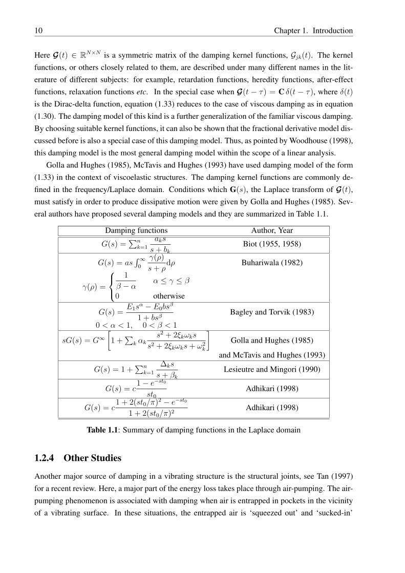
is the Dirac-delta function, equation (1.33) reduces to the case of viscous damping as in equation(1.30). The damping model of this kind is a further generalization of the familiar viscous damping.By choosing suitable kernel functions, it can also be shown that the fractional derivative model dis-cussed before is also a special case of this damping model. Thus, as pointed by Woodhouse (1998),this damping model is the most general damping model within the scope of a linear analysis.
Golla and Hughes (1985), McTavis and Hughes (1993) have used damping model of the form(1.33) in the context of viscoelastic structures. The damping kernel functions are commonly de-fined in the frequency/Laplace domain. Conditions which G(s), the Laplace transform of G(t),must satisfy in order to produce dissipative motion were given by Golla and Hughes (1985). Sev-eral authors have proposed several damping models and they are summarized in Table 1.1.
Damping functions Author, Year
G(s) =∑n
k=1
aks
s + bk
Biot (1955, 1958)
G(s) = as∫∞0
γ(ρ)
s + ρdρ Buhariwala (1982)
γ(ρ) =
1
β − αα ≤ γ ≤ β
0 otherwise
G(s) =E1s
α − E0bsβ
1 + bsβBagley and Torvik (1983)
0 < α < 1, 0 < β < 1
sG(s) = G∞[1 +
∑k αk
s2 + 2ξkωks
s2 + 2ξkωks + ω2k
]Golla and Hughes (1985)
and McTavis and Hughes (1993)
G(s) = 1 +∑n
k=1
∆ks
s + βk
Lesieutre and Mingori (1990)
G(s) = c1− e−st0
st0Adhikari (1998)
G(s) = c1 + 2(st0/π)2 − e−st0
1 + 2(st0/π)2Adhikari (1998)
Table 1.1: Summary of damping functions in the Laplace domain
1.2.4 Other Studies
Another major source of damping in a vibrating structure is the structural joints, see Tan (1997)for a recent review. Here, a major part of the energy loss takes place through air-pumping. The air-pumping phenomenon is associated with damping when air is entrapped in pockets in the vicinityof a vibrating surface. In these situations, the entrapped air is ‘squeezed out’ and ‘sucked-in’

1.3. Modal Analysis of Viscously Damped Systems 11
through any available hole. Dissipation of energy takes place in the process of air flow and culomb-friction dominates around the joints. This damping behaviour has been studied by many authorsin some practical situations, for example by Cremer and Heckl (1973). Earls (1966) has obtainedthe energy dissipation in a lap joint over a cycle under different clamping pressure. Beards andWilliams (1977) have noted that significant damping can be obtained by suitably choosing thefastening pressure at the interfacial slip in joints.
Energy dissipation within the material is attributed to a variety of mechanisms such as thermoe-lasticity, grainboundary viscosity, point-defect relaxation etc (see Lazan, 1959, 1968, Bert, 1973).Such effects are in general called material damping. In an imperfect elastic material, the stress-strain curve forms a closed hysteresis loop rather that a single line upon a cyclic loading. Mucheffort has been devoted by numerous investigators to develop models of hysteretic restoring forcesand techniques to identify such systems. For a recent review on this literature we refer the readersto Chassiakos et al. (1998). Most of these studies are motivated by the observed fact that the energydissipation from materials is only a weak function of frequency and almost directly proportional toxn. The exponent on displacement for the energy dissipation of material damping ranges from 2 to3, for example 2.3 for mild steel (Bandstra, 1983). In this context, another large body of literaturecan be found on composite materials where many researchers have evaluated a material’s specificdamping capacity (SDC). Baburaj and Matsukai (1994) and the references therein give an accountof research that has been conducted in this area.
1.3 Modal Analysis of Viscously Damped Systems
Equations of motion of a viscously damped system can be obtained from the Lagrange’s equation(1.7) and using the Rayleigh’s dissipation function given by (1.30). The non-conservative forcescan be obtained as
Qnck= −∂F
∂qk
, k = 1, · · · , N (1.34)
and consequently the equations of motion can expressed as
Mq(t) + Cq(t) + Kq(t) = f(t). (1.35)
The aim is to solve this equation (together with the initial conditions) by modal analysis as de-scribed in Section 1.1.2. Using the transformation in (1.14), premultiplying equation (1.35) by XT
and using the orthogonality relationships in (1.12) and (1.13), equations of motion of a dampedsystem in the modal coordinates may be obtained as
y(t) + XT CXy(t) + Ω2y(t) = f(t). (1.36)
Clearly, unless XT CX is a diagonal matrix, no advantage can be gained by employing modalanalysis because the equations of motion will still be coupled. To solve this problem, it it common

12 Chapter 1. Introduction
to assume proportional damping, that is C is simultaneously diagonalizable with M and K. Suchdamping model allows to analyze damped systems in very much the same manner as undampedsystems. Later, Caughey and O’Kelly (1965) have derived the condition which the system matricesmust satisfy so that viscously damped linear systems possess classical normal modes. In Chapter2, the concept of proportional damping or classical damping will be analyzed in more detail.
Modes of proportionally damped systems preserve the simplicity of the real normal modes as inthe undamped case. Unfortunately there is no physical reason why a general system should behavelike this. In fact practical experience in modal testing shows that most real-life structures do not doso, as they possess complex modes instead of real normal modes. This implies that in general linearsystems are non-classically damped. When the system is non-classically damped, some or all ofthe N differential equations in (1.36) are coupled through the XT CX term and can not be reducedto N second-order uncoupled equation. This coupling brings several complication in the systemdynamics – the eigenvalues and the eigenvectors no longer remain real and also the eigenvectorsdo not satisfy the classical orthogonality relationship as given by equations (1.10) and (1.11). Themethods for solving this kind of problem follow mainly two routes, the state-space method and themethods in configuration space or ‘N -space’. A brief discussion of these two approaches is takenup in the following sections.
1.3.1 The State-Space Method
The state-space method is based on transforming the N second-order coupled equations into aset of 2N first-order coupled equations by augmenting the displacement response vectors with thevelocities of the corresponding coordinates (see Newland, 1989). Equation (1.35) can be recast as
z(t) = Az(t) + p(t) (1.37)
where A ∈ R2N×2N is the system matrix, p(t) ∈ R2N the force vector and z(t) ∈ R2N is theresponse vector in the state-space given by
A =
[ON IN
−M−1K −M−1C
], z(t) =
q(t)q(t)
, and p(t) =
0
−M−1f(t).
(1.38)
In the above equation ON is the N × N null matrix and IN is the N × N identity matrix. Theeigenvalue problem associated with the above equation is in term of an asymmetric matrix now.Uncoupling of equations in the state-space is again possible and has been considered by manyauthors, for example, Meirovitch (1980), Newland (1989) and Veletsos and Ventura (1986). Thisanalysis was further generalized by Newland (1987) for the case of systems involving singularmatrices. In the formulation of equation (1.37) the matrix A is no longer symmetric, and so eigen-vectors are no longer orthogonal with respect to it. In fact, in this case, instead of an orthogonalityrelationship, one obtains a biorthogonality relationship, after solving the adjoint eigenvalue prob-lem. The complete procedure for uncoupling the equations now involves solving two eigenvalue

1.3. Modal Analysis of Viscously Damped Systems 13
problems, each of which is double the size of an eigenvalue problem in the modal space. The de-tails of the relevant algebra can be found in Meirovitch (1980, 1997). It should be noted that thesesolution procedures are exact in nature. One disadvantage of such an exact method is that it re-quires significant numerical effort to determine the eigensolutions. The effort required is evidentlyintensified by the fact that the eigensolutions of a non-classically damped system are complex.From the analyst’s view point another disadvantage is the lack of physical insight afforded by thismethod which is intrinsically numerical in nature.
Another variation of the state-space method available in the literature is through the use of‘Duncan form’. This approach was introduced by Foss (1958) and later several authors, for ex-ample, Beliveau (1977), Nelson and Glasgow (1979), Vigneron (1986), Suarez and Sing (1987,1989), Sestieri and Ibrahim (1994) and Ren and Zheng (1997) have used this approach to solve awide range of interesting problems. The advantage of this approach is that the system matrices inthe state-space retain symmetry as in the configuration space.
1.3.2 Methods in Configuration Space
It has been pointed out that the state-space approach towards the solution of equation of motionin the context of linear structural dynamics is not only computationally expensive but also fails toprovide the physical insight which modal analysis in configuration space or N -space offers. Theeigenvalue problem associated with equation (1.35) can be represented by the λ−matrix problem(Lancaster, 1966)
s2jMuj + sjCuj + Kuj = 0 (1.39)
where sj ∈ C is the j-th latent root (eigenvalue) and uj ∈ CN is the j-th latent vector (eigenvector).The eigenvalues, sj , are the roots of the characteristic polynomial
det[s2M + sC + K
]= 0. (1.40)
The order of the polynomial is 2N and the roots appear in complex conjugate pairs. Several authorshave studied non-classically damped linear systems by approximate methods. In this section webriefly review the existing methods for this kind of analysis.
Approximate Decoupling Method
Consider the equations of motion of a general viscously damped system in the modal coordinatesgiven by (1.36). Earlier it has been mentioned that due to non-classical nature of the damping thisset of N differential equations are coupled through the C′ = XT CX term. An usual approach inthis case is simply to ignore the off-diagonal terms of the modal damping matrix C′ which couplethe equations of motion. This approach is termed the decoupling approximation. For large-scalesystems, the computational effort in adopting the decoupling approximation is an order of magni-tude smaller than the methods of complex modes. The solution of the decoupled equation would

14 Chapter 1. Introduction
be close to the exact solution of the coupled equations if the non-classical damping terms are suffi-ciently small. Analysis of this question goes back to Rayleigh (1877). A preliminary discussion onthis topic can be found in Meirovitch (1967, 1997). Thomson et al. (1974) have studied the effectof neglecting off-diagonal entries of the modal damping matrix through numerical experiments andhave proposed a method for improved accuracy. Warburton and Soni (1977) have suggested a cri-terion for such a diagonalization so that the computed response is acceptable. Using the frequencydomain approach, Hasselsman (1976) proposed a criterion for determining whether the equationsof motion might be considered practically decoupled if non-classical damping exists. The criterionsuggested by him was to have adequate frequency separation between the natural modes.
Using matrix norms, Shahruz and Ma (1988) have tried to find an optimal diagonal matrixCd in place of C′. An important conclusion emerging from their study is that if C′ is diagonallydominant, then among all approximating diagonal matrices Cd, the one that minimizes the errorbound is simply the diagonal matrix obtained by omitting the off-diagonal elements of C′. Usinga time-domain analysis Shahruz (1990) has rigorously proved that if Cd is obtained form C′ byneglecting the off-diagonal elements of C′, then the error in the solution of the approximatelydecoupled system will be small as long as the off-diagonal elements of C′ are not too large.
Ibrahimbegovic and Wilson (1989) have developed a procedure for analyzing non-pro- portion-ally damped systems using a subspace with a vector basis generated from the mass and stiffnessmatrices. Their approach avoids the use of complex eigensolutions. An iterative approach forsolving the coupled equations is developed by Udwadia and Esfandiari (1990) based on updatingthe forcing term appropriately. Felszeghy (1993) presented a method which searches for anothercoordinate system in the neighborhood of the normal coordinate system so that in the new coordi-nate system removal of coupling terms in the equations of motion produces a minimum bound onthe relative error introduced in the approximate solution. Hwang and Ma (1993) have shown thatthe error due to the decoupling approximation can be decomposed into an infinite series and canbe summed exactly in the Laplace domain. They also concluded that by solving a small number ofadditional coupled equations in an iterative fashion, the accuracy of the approximate solution canbe greatly enhanced. Felszeghy (1994) developed a formulation based on biorthonormal eigen-vector for modal analysis of non-classically damped discrete systems. The analytical proceduretake advantage of simplification that arises when the modal analysis of the motion separated into aclassical and non-classical modal vector expansion.
From the above mentioned studies it has been believed that either frequency separation be-tween the normal modes (Hasselsman, 1976), often known as ‘Hasselsman’s criteria’, or someform of diagonal dominance (Shahruz and Ma, 1988), in the modal damping matrix C′ is sufficientfor neglecting modal coupling. In contrast to these widely accepted beliefs Park et al. (1992a,b,1994) have shown using Laplace transform methods that within the practical range of engineeringapplications neither the diagonal dominance of the modal damping matrix nor the frequency sep-aration between the normal modes would be sufficient for neglecting modal coupling. They have

1.3. Modal Analysis of Viscously Damped Systems 15
also given examples when the effect of modal coupling may even increase following the previouscriterion.
In the context of approximate decoupling, Shahruz and Srimatsya (1997) have considered errorvectors in modal and physical coordinates, say denoted by eN(•) and eP(•) respectively. Theyhave shown that based on the norm (denoted here as ‖ (•) ‖) of these error vectors three cases mayarise:
1. ‖ eN(•) ‖ is small (respectively, large) and ‖ eP(•) ‖ is small (respectively, large)
2. ‖ eN(•) ‖ is large but ‖ eP(•) ‖ is small
3. ‖ eN(•) ‖ is small but ‖ eP(•) ‖ is large
From this study, especially in view of case 3, it is clear that the error norms based on the modalcoordinates are not reliable to use in the actual physical coordinates. However, they have givenconditions when ‖ eN(•) ‖ will lead to a reliable estimate of ‖ eP(•) ‖. For a flexible structurewith light damping, Gawronski and Sawicki (1997) have shown that neglecting off-diagonal termsof the modal damping matrix in most practical cases imposes negligible errors in the system dy-namics. They also concluded that the requirement of diagonal dominance of the damping matrixis not necessary in the case of small damping, which relaxes the criterion earlier given by Shahruzand Ma (1988).
In order to quantify the extent of non-proportionality, several authors have proposed ‘non-proportionality indices’. Parter and Sing (1986) and Nair and Sing (1986) have developed sev-eral indices based on modal phase difference, modal polygon areas, relative magnitude of cou-pling terms in the modal damping matrix, system response, Nyquist plot etc. Recently, basedon the idea related to the modal polygon area, Bhaskar (1999) has proposed two more indicesof non-proportionality. Another index based on driving frequency and elements of the modaldamping matrix is given by Bellos and Inman (1990). Bhaskar (1992, 1995) has proposed a non-proportionality index based on the error introduced by ignoring the coupling terms in the modaldamping matrix. Tong et al. (1992, 1994) have developed an analytical index for quantification ofnon-proportionality for discrete vibrating systems. It has been shown that the fundamental natureof non-proportionality lies in finer decompositions of the damping matrix. Shahruz (1995) haveshown that the analytical index given by Tong et al. (1994) solely based on the damping matrix canlead to erroneous results when the driving frequency lies close to a system natural frequency. Theyhave suggested that a suitable index for non-proportionality should include the damping matrixand natural frequencies as well as the excitation vector. Prells and Friswell (2000) have shown thatthe (complex) modal matrix of a non-proportionally damped system depends on an orthonormalmatrix, which represents the phase between different degrees of freedom of the system. For pro-portionally damped systems this matrix becomes an identity matrix and consequently they haveused this orthonormal matrix as an indicator of non-proportionality. Recently, Liu et al. (2000) has

16 Chapter 1. Introduction
proposed three indices to measure the damping non-proportionality. The first index measures thecorrelation between the real and imaginary parts of the complex modes, the second index measuresthe magnitude of the imaginary parts of the complex modes and the third index quantifies the de-gree of modal coupling. These indices are based on the fact that the complex modal matrix can bedecomposed to a product of a real and and complex matrix.
Complex Modal Analysis
Other than the approximate decoupling methods, another approach towards the analysis of non-proportionally damped linear systems is to use complex modes. Since the original contributionof Caughey and O’Kelly (1965), many papers have been written on complex modes. Several au-thors, for example, Mitchell (1990), Imregun and Ewins (1995) and Lallement and Inman (1995),have given reviews on this subject. Placidi et al. (1991) have used a series expansion of complexeigenvectors into the subspace of real modes, in order to identify normal modes from complexeigensolutions. In the context of modal analysis Liang et al. (1992) have posed and analyzed thequestion of whether the existence of complex modes is an indicator of non-proportional dampingand how a mode is influenced by damping. Analyzing the errors in the use of modal coordinates,Sestieri and Ibrahim (1994) and Ibrahim and Sestieri (1995) have concluded that the complex modeshapes are not necessarily the result of high damping. The complexity of the mode shapes is theresult of particular damping distributions in the system and depends upon the proximity of themode shapes. Liu and Sneckenberger (1994) have developed a complex mode theory for a linearvibrating deficient system based on the assumption that it has a complete set of eigenvectors. Com-plex mode superposition methods have been used by Oliveto and Santini (1996) in the context ofsoil structure interaction problems. Balmes (1997) has proposed a method to find normal modesand the associated non-proportional damping matrix from the complex modes. He has also shownthat a set of complex modes is complete if it verifies a defined properness condition which is usedto find complete approximations of identified complex modes. Garvey et al. (1995) have given arelationship between real and imaginary parts of complex modes for general systems whose mass,stiffness and damping can be expressed by real symmetric matrices. They have also observed thatthe relationship becomes most simple when all roots are complex and the real part of all the rootshave same sign. Recently Bhaskar (1999) has analyzed complex modes in detail and addressed theproblem of visualizing the deformed modes shapes when the motion is not synchronous.
While the above mentioned works concentrate on the properties of the complex modes, severalauthors have considered the problem of determination of complex modes in the N -space. Cronin(1976) has obtained an approximate solution for a non-classically damped system under harmonicexcitation by perturbation techniques. Clough and Mojtahedi (1976) considered several methodsof treating generally damped systems, and concluded that the proportional damping approxima-tion may give unreliable results for many cases. Similarly, Duncan and Taylor (1979) have shownthat significant errors can be incurred when dynamic analysis of a non-proportionally damped sys-

1.3. Modal Analysis of Viscously Damped Systems 17
tem is based on a truncated set of modes, as is commonly done in modelling continuous systems.Meirovitch and Ryland (1985) have used a perturbation approach to obtain left and right eigen-vectors of damped gyroscopic systems. Chung and Lee (1986) applied perturbation techniques toobtain the eigensolutions of damped systems with weakly non-classical damping. Cronin (1990)has developed an efficient perturbation-based series method to solve the eigenproblem for dynamicsystems having non-proportional damping matrix. To illustrate the general applicability of thismethod, Peres-Da-Silva et al. (1995) have applied it to determine the eigenvalues and eigenvectorsof a damped gyroscopic system. In the context of non-proportionally damped gyroscopic systemsMalone et al. (1997) have developed a perturbation method which uses an undamped gyroscopicsystem as the unperturbed system. Based on a small damping assumption, Woodhouse (1998)has given the expression for complex natural frequencies and mode shapes of non-proportionallydamped linear discrete systems with viscous and non-viscous damping. More recently, based onthe idea related to the first-order perturbation method, Adhikari (2000) has proposed an expressionof complex modes in terms of classical normal modes.
Response Bounds and Frequency Response
In the two previous subsections we have mainly discussed on the eigensolutions of non-classicallydamped systems. In this subsection we briefly consider the problem of obtaining dynamic responseof such systems. Nicholson (1987b) and Nicholson and Baojiu (1996) have reviewed the literatureon stable response of non-classically damped mechanical systems. Nicholson (1987a) gave upperbounds for the response of non-classically damped systems under impulsive loads and step loads.Yae and Inman (1987) have obtained bound on the displacement response of non-proportionallydamped discrete systems in terms of physical parameters of the system and input. They also haveobserved that the larger the deviation from proportional damping the less accurate their resultsbecome.
Bellos and Inman (1990) have given a procedure for computing the transfer functions of anon-proportionally damped discrete system. Their method was based on Laplace transformationof the equation of motion in modal coordinates. A fairly detailed survey of the previous research ismade in Bellos and Inman (1990). Yang (1993) has developed a iterative procedure for calculationof the transfer functions of non-proportionally damped systems. Bhaskar (1995) has analyzedthe behaviour of errors in calculating frequency response function when the off-diagonal terms ofmodal damping matrix are neglected. It has been shown that the exact response can be expressedby an infinite Taylor series and the approximation of ignoring the off-diagonal terms of modaldamping matrix is equivalent to retaining one term of the series.
Finally, it should be noted that frequency responses of viscously damped systems with non-proportional damping can be obtained exactly in terms of the complex frequencies and complexmodes in the configuration space, see for example Lancaster (1966, Section 7.5) and Geradin andRixen (1997, pp. 126-128). Similar expressions are also derived by Fawzy and Bishop (1976),

18 Chapter 1. Introduction
Vigneron (1986) and Woodhouse (1998). This in turn requires determination of complex modes inthe configuration space.
1.4 Analysis of Non-viscously Damped Systems
In Section 1.2.3 it was pointed out that the most general way to model (non-viscous) dampingwithin the scope of linear theory is through the use of the modified dissipation function given byequation (1.33). Equations of motion of such non-viscously damped systems can be obtained fromthe Lagrange’s equation (1.7). The non-conservative forces can be obtained as
Qnck= −∂F
∂qk
= −N∑
j=1
∫ t
0
Gjk(t− τ)qj(τ)dτ, k = 1, · · · , N (1.41)
and consequently the equations of motion can be expressed as
Mq(t) +
∫ t
0
G(t− τ)q(τ)dτ + Kq(t) = f(t). (1.42)
This is a set of coupled second-order integro-differential equation. The presence of the ‘integral’term in the equations of motion complicates the analysis. Unlike the viscously damped systems,the concept of ‘proportional damping’ cannot easily be formulated for such systems. The questionof the existence of classical normal modes in such systems, i.e., if proportional damping can occurin such systems, will be discussed in Chapter 2.
Equations similar to (1.42) occur in many different subjects. Bishop and Price (1979) haveconsidered equations of motion similar to (1.42) in the context of ship dynamics. The convolutionterm appeared in order to represent the fluid forces and moments. They have discussed the eigen-value problem associated with equation (1.42) and presented an orthogonality relationship for theright and left eigenvectors. They have also given an expression for the system response due to sinu-soidal excitation. Their results were not very efficient because the orthogonality relationship of theeigenvectors were not utilized due to the difficulty associated with the form of the orthogonalityequation, which itself became frequency dependent.
Equations of motion like (1.42) also arise in the dynamics of viscoelastic structures. Gollaand Hughes (1985), McTavis and Hughes (1993) have proposed a method to obtain such equationsusing a time-domain finite-element formulation. Their approach (the GHM method), which intro-duces additional dissipation coordinates corresponding to the internal dampers, increases the sizeof the problem. Dynamic responses of the system were obtained by using the eigensolutions of theaugmented problem in the state-space. Muravyov (1997, 1998) has proposed a method to obtainthe time and frequency-domain description of the response by introducing additional coordinateslike the GHM method. To reduce the order of the problem, recently Park et al. (1999) and Friswelland Inman (1999) have proposed a state-space approach which employs a modal truncation anduses an iterative approach to obtain the eigensolutions. Using a first-order perturbation approach,

1.5. Identification of Viscous Damping 19
Woodhouse (1998) has obtained expressions for the eigensolutions and transfer functions of system(1.42). His method, although it avoids the state-space representations and additional dissipationcoordinates, is valid for small damping terms only.
1.5 Identification of Viscous Damping
In Section 1.3 we have discussed several methods for analysis of viscously damped linear dynamicsystems. In this section we focus our attention on the methodologies available for identification ofviscous damping parameters from experimental measurements.
1.5.1 Single Degree-of-freedom Systems Systems
Several methods are available for identifying the viscous damping parameters for single degree offreedom systems for linear and non-linear damping models (see Nashif et al., 1985). For lineardamping models these methods can be broadly described as:
1. Methods based on transient response of the system: This is also known as logarithmic decre-ment method: if qi and qi+i are heights of two subsequent peaks then the damping ratio ζ
can be obtained asδ = loge
(qi
qi+i
)≈ 2πζ (1.43)
For applicability of this method the decay must be exponential.
2. Methods based on harmonic response of the system: These methods are based on calculatingthe half power points and bandwidth from the frequency response curve. It can be shown thatthe damping factor ζ can be related to a peak of the normalized frequency response curve by
|H|max ≈ 1
2ζ(1.44)
3. Methods based on energy dissipation: Consider the force-deflection behaviour of a spring-mass-damper (equivalent to a block of material) under sinusoidal loading at some particularfrequency. In steady-state, considering conservation of energy, energy loss per cycle (∆ucyc)can be calculated by equating it with the input power. Here it can be shown that the dampingfactor ζ can be related as
2ζ =∆ucyc
2πUmax
(1.45)
where Umax is maximum energy of the system.
The above mentioned methods, although developed for single-degree-of-freedom systems, can beused for separate modes of multiple degree of freedom systems, for example a cantilever beamvibrating in the first mode. Recently Chassiakos et al. (1998) proposed an on-line parameter iden-tification technique for a single degree of freedom hysteretic system.

20 Chapter 1. Introduction
1.5.2 Multiple Degrees-of-freedom Systems
For multiple degree-of-freedom systems, most of the common methods for experimental determi-nation of the damping parameters use the proportional damping assumption. A typical procedurecan be described as follows (see Ewins, 1984, for details):
1. Measure a set of transfer functions Hij(ω) at a set of grid points on the structure.
2. Obtain the natural frequencies ωk by a pole-fitting method.
3. Evaluate the modal half-power bandwidth ∆ωk from the frequency response functions, thenthe Q-factor Qk = ωk
∆ωkand the modal damping factor ζk = 1
2Qk.
4. Determine the modal amplitude factors ak to obtain the mode shapes, uk.
5. Finally reconstruct some transfer functions to verify the accuracy of the evaluated parame-ters.
Such a procedure does not provide reliable information about the nature or spatial distribution ofthe damping, though the reconstructed transfer functions may match the measured ones well.
The next stage, followed by many researchers, is to attempt to obtain the full viscous dampingmatrix from the experimental measurements. Pilkey and Inman (1998) have given a recent surveyon methods of viscous damping identification. These methods can be divided into two basic cate-gories (Fabunmi et al., 1988): (a) damping identification from modal testing and analysis, and (b)direct damping identification from the forced response measurements.
The modal testing and analysis method seeks to determine the modal parameters, such as nat-ural frequencies, damping ratio and mode shapes, from the measured transfer functions, and thenfit a damping matrix to these data. In one of the earliest works, Lancaster (1961) has given anexpression from which the damping matrix can be constructed from complex modes and frequen-cies. Unfortunately this expression relies on having all the modes, which is almost impossiblein practice. For this reason, several authors have proposed identification methods by consider-ing the modal data to be incomplete or noisy. Hasselsman (1972) has proposed a perturbationmethod to identify a non-proportional viscous damping matrix from complex modes and frequen-cies. Beliveau (1976) has proposed a method which uses eigensolutions, phase angles and dampingratios to identify the parameters of viscous damping matrix. His method utilizes a Bayesian frame-work based on eigensolution perturbation and a Newton-Raphson scheme. Ibrahim (1983b) usesthe higher order analytical modes together with the experimental set of complex modes to computeimproved mass, stiffness and damping matrices. Minas and Inman (1991) have proposed a methodfor viscous damping identification in which it is assumed that the mass and stiffness are a priori
known and modal data, obtained from experiment, allowed to be incomplete. Starek and Inman(1997) have proposed an inverse vibration problem approach in which it is assumed that the damp-ing matrix has an a priori known structure. Their method yields a positive-definite damping matrix

1.6. Identification of Non-viscous Damping 21
but requires the full set of complex modes. Pilkey and Inman (1997) have developed an iterativemethod for damping matrix identification by using Lancaster’s (1961) algorithm. This method re-quires experimentally identified complex eigensolutions and the mass matrix. Alvin et al. (1997)have proposed a method in which a correction was applied to the proportionally damped matrix bymeans of an error minimization approach. Recently Halevi and Kenigsbuch (1999) have proposeda method for updating the damping matrix by using the reference basis approach in which error andincompleteness of the measured modal data were taken into account. As an intermediate step, theirmethod corrects the imaginary parts of the measured complex modes which are more inaccuratethan their corresponding real parts.
Direct damping identification methods attempt to fit the equations of motion to the measuredforced response data at several time/frequency points. Caravani and Thomson (1974) have pro-posed a least-square error minimization approach to obtain the viscous damping matrix. Theirmethod uses measured frequency response at a set of chosen frequency points and utilizes an it-erative method to successively improve the identified parameters. Fritzen (1986) has used theinstrumental variable method for identification of the mass, damping and stiffness matrices. It wasobserved that the identified values are less sensitive to noise compared to what obtained from least-square approach. Fabunmi et al. (1988) has presented a damping matrix identification scheme thatuses forced response data in the frequency domain and assumes that the mass and stiffness ma-trices are known. Mottershead (1990) has used the inverse of the frequency response functionsto modify the system matrices so that the modified model varies minimally from an initial finite-element model. Using a different approach, Roemer and Mook (1992) have developed methodsin the time domain for simultaneous identification of the mass, damping and stiffness matrices. Itwas observed that the identified damping matrix has larger relative error than that of the mass andstiffness matrices. Chen et al. (1996a) have proposed a frequency domain technique for identifi-cation of the system matrices in which the damping matrix was determined independently. It wasshown that separate identification of the damping matrix improves the result as relative magnitudeof the damping matrix is less than those of the mass and stiffness matrices. Later, Baruch (1997)has proposed a similar approach in which the damping matrix was identified separately from themass and stiffness matrices.
1.6 Identification of Non-viscous Damping
Unlike viscous damping, there is very little available in the literature which discusses genericmethodologies for identification of non-viscous damping. Most of the methods proposed in theliterature are system-specific. Banks and Inman (1991) have considered the problem of estimatingdamping parameters in a non-proportionally damped beam. They have taken four different mod-els of damping: viscous air damping, Kelvin-Voigt damping, time hysteresis damping and spatialhysteresis damping, and used a spline inverse procedure to form a least-square fit to the experimen-

22 Chapter 1. Introduction
tal data. A procedure for obtaining hysteretic damping parameters in free-hanging pipe systemsis given by Fang and Lyons (1994). Assuming material damping is the only source of dampingthey have given a theoretical expression for the loss factor of the n-th mode. Their theory pre-dicts higher modal damping ratios in higher modes. Maia et al. (1997) have emphasized the needfor development of identification methodologies of general damping models and indicated severaldifficulties that might arise. Recently, Dalenbring (1999) has proposed a method for identificationof (exponentially decaying) damping functions from the measured frequency response functionsand finite element displacement modes. A limitation of this method is that it neglects the effect ofmodal coupling, that is, the identified non-viscous damping model is effectively proportional.
1.7 Open Problems
From the discussions based on the existing literature it is clear that in spite of extensive research ef-fort, many questions regarding damped dynamic systems are still to be answered. These questionscan be broadly divided as follows:
1. What damping model has to be used for a given structure, i.e., viscous or non-viscous, andif non-viscous then what kind of model should it be?
2. How can conventional modal analysis be extended to systems with non-viscous damping?
3. How is it possible to determine the damping parameters by conventional modal testing if asystem is non-viscous?
The first question is a major issue, and in the context of general vibration analysis, has been ‘set-tled’ by assuming viscous damping, although has been pointed out in the literature that in generalit will not be the correct model. The last two questions are related to each other in the sense thatfor identification of the non-viscous damping parameters a reliable method of modal analysis isalso required.
Most of the techniques for detecting damping in a structure either consider the structure to beviscously damped or a priori assume some particular non-viscous model of damping and try to fitits parameters with regard to some specific structure. This a priori selection of damping no doubthides the physics of the system and there has not been any indication in the literature on how to finda damping model by doing conventional vibration testing. However another relevant question inthis context is whether this a priori selection of damping model matters from an engineering pointof view: it may be possible that a pre-assumed damping model with a ‘correct’ set of parametersmay represent the system response quite well, although the actual physical mechanism behind thedamping may be different. These issues will be discussed in this dissertation. Next, the workstaken up in this dissertation is outlined briefly.
1.8. Outline of the Dissertation 23
1.8 Outline of the Dissertation
Motivated by the existing gaps and open problems identified in the last section, a systematic studyon analysis and identification of damped discrete linear dynamic systems has been carried out inthis dissertation. In Section 1.2 it has been brought out that the convolution integral model is themost general damping model for multiple-degrees-of-freedom linear systems. Attention is specif-ically focused on this kind of general damping model. However, for comparing and establishingthe relationship with the current literature, viscously damped systems are also discussed. Thedissertation is divided into nine chapters and two Appendices.
In Chapter 2, the concept of classical damping, well known for viscously damped systems,is extended to non-viscously damped discrete linear systems. The convolution integral model isassumed for non-viscous damping. Conditions for the existence of classical normal modes insuch non-viscously damped systems are discussed. Several numerical examples are provided toillustrate the derived results.
Chapter 3 is aimed at extending classical modal analysis to treat lumped-parameter non-viscouslydamped linear dynamic systems. The nature of the eigenvalues and eigenvectors are discussedunder certain simplified but physically realistic assumptions concerning the system matrices andkernel functions. A numerical method for calculation of the eigenvectors is suggested. The transferfunction matrix of the system is derived in terms of the eigenvectors of the second-order system.Exact closed-form expressions for the dynamic response due to general forces and initial condi-tions are derived.
In Chapter 4, the mode-orthogonality relationships, known for undamped or viscously dampedsystems, have been generalized to such non-viscously damped systems. Some expressions aresuggested for the normalization of the eigenvectors. A number of useful results which relate thesystem matrices with the eigensolutions have been established.
The above mentioned studies give a firm basis for modal analysis of non-viscously dampedsystems. Motivated by these results, from Chapter 5 onwards, studies on damping identificationare considered. Chapter 5 considers identification of viscous damping under circumstances whenthe actual damping model in the structure is non-viscous. A method is presented to obtain a full(non-proportional) viscous damping matrix from complex modes and complex natural frequencies.It is assumed that the damping is ‘small’ so that a first order perturbation method is applicable.The proposed method and several related issues are discussed by considering numerical examplesbased on a linear array of damped spring-mass oscillators. It is shown that the method can predictthe spatial location of damping with good accuracy, and also give some indication of the correctmechanism of damping.
From the studies in Chapter 5 it is observed that when a system is non-viscously damped, anidentified equivalent viscous damping model does not accurately represent the damping behaviour.This demands new methodologies to identify non-viscous damping models. Chapter 6 takes a

24 Chapter 1. Introduction
first step, by outlining a procedure for identifying a damping model involving an exponentially-decaying relaxation function. The method uses experimentally identified complex modes and com-plex natural frequencies, together with the knowledge of mass matrix for the system. The proposedmethod and several related issues are discussed by considering numerical examples of a linear ar-ray of damped spring-mass oscillators. It is shown that good estimates can be obtained for theexponential time constant and the spatial distribution of the damping.
In some cases the identified damping matrix become non-symmetric, which in a way is a non-physical result because the original system is reciprocal. In Chapter 7, methods are developedto identify damping models which preserve the symmetry of the system. Both viscous and non-viscous models are considered. The procedures are based on a constrained error minimizationapproach and they use experimentally identified complex modes and complex natural frequencies.The proposed methods are supported by suitable numerical examples.
Experimental verification of the damping identification techniques developed in this disserta-tion is considered in Chapter 8. First, extraction of complex modes and frequencies from a set ofmeasured transfer functions is considered as all the damping identification procedures rely heav-ily on these complex modal parameters. A general methodology based on linear-nonlinear least-square approach is proposed. The experimental structure is comprised of a beam with localizedconstrained layer damping. It is demonstrated that the proposed approach for damping identifica-tion can indeed predict the nature of the damping with good accuracy. Through an error analysis,it is further shown that the proposed method is likely to be robust in the presence of noisy data,as the identified damping matrix is less sensitive to the imaginary parts of the complex modes, onwhich any measurement noise has highest effect.
Finally, Chapter 9 presents the conclusions emerging from the studies taken up in this disserta-tion and makes a few suggestions for further research.

Chapter 2
The Nature of Proportional Damping
2.1 Introduction
Modal analysis is the most popular and efficient method for solving engineering dynamic problems.The concept of modal analysis, as introduced by Rayleigh (1877), was originated from the lineardynamics of undamped systems. It was shown (see Section 1.1.2 for details) that the undampedmodes or classical normal modes satisfy an orthogonality relationship over the mass and stiffnessmatrices and uncouple the equations of motion, i.e., If X ∈ RN×N is the modal matrix then XT MXand XT KX are both diagonal matrices. This significantly simplifies the dynamic analysis becausecomplex multiple degree-of-freedom (MDOF) systems can be treated as a collection of singledegree-of-freedom oscillators.
Real-life systems are however, not undamped, but possess some kind of energy dissipationmechanism or damping. In order to apply modal analysis of undamped systems to damped sys-tems, it is common to assume the proportional damping, a special case of viscous damping. Theproportional damping model expresses the damping matrix as a linear combination of the mass andstiffness matrices, that is
C = α1M + α2K (2.1)
where α1, α2 are real scalars. This damping model is also known as ‘Rayleigh damping’ or ‘clas-sical damping’. Modes of classically damped systems preserve the simplicity of the real normalmodes as in the undamped case. Caughey and O’Kelly (1965) have derived the condition whichthe system matrices must satisfy so that viscously damped linear systems possess classical normalmodes. They have also proposed an (series) expression for the damping matrix in terms of themass and stiffness matrices so that the system can be decoupled by the undamped modal matrixand have shown that the Rayleigh damping is a special case of this general expression. In thischapter a more general expression of the damping matrix is proposed so that the system possessclassical normal modes.
There are no physical reasons to believe that viscous damping is the only linear damping model.It is perfectly possible for the damping forces to depend on values of other quantities. In the last
25

26 Chapter 2. The Nature of Proportional Damping
chapter (see Section 1.2.3) it was concluded that the convolution integral model is the most generallinear damping model. Since the concept of classical or proportional damping is defined in thecontext of viscously damped systems, it is not clear whether such a concept exists for this kind ofnon-viscously damped systems. In this chapter we address the question – under what conditionscan such non-viscously damped systems be ‘classically damped’? i.e., under what conditions suchnon-viscously damped systems possess classical normal modes?
2.2 Viscously Damped Systems
The equations of motion of free vibration of a viscously damped system can be expressed by
Mq(t) + Cq(t) + Kq(t) = 0. (2.2)
In this case the equations of motion are characterized by three real symmetric matrices whichbrings additional complication compared to the undamped systems where the equations of motionare characterized by two matrices. We require a non-zero matrix X ∈ RN×N such that it simulta-neously diagonalizes M, C and K under a congruence transformation. This requirement restrictsthe admissible forms of these matrices as discussed below.
2.2.1 Existence of Classical Normal Modes
Caughey and O’Kelly (1965) have proved that a damped linear system of the form (2.2) can pos-sess classical normal modes if and only if the system matrices satisfy the relationship KM−1C =
CM−1K. This is an important result on modal analysis of viscously damped systems and is nowwell known. However, this result does not immediately generalize to systems with singular massmatrices (see Newland, 1989, Chapter 6). This apparent restriction in Caughey and O’Kelly’s re-sult may be removed by considering the fact that the properties (and roles) of all the three systemmatrices are identical and can be treated on equal basis. In view of this, a modified version ofCaughey and O’Kelly’s theorem can be stated as following:Theorem 2.1. If M, C and K are positive definite matrices and there exist a nonsingular X ∈RN×N such that XT MX, XT CX and XT KX are all real diagonal matrices then the following are
equivalent
(a) KM−1C = CM−1K, (b) MK−1C = CK−1M, (c) MC−1K = KC−1M.
Proof. We have to prove that: (1) from the given condition (a), (b) and (c) follows, (2) from (a),(b) and (c) the given condition follows – in total all the six statements proposed in the theorem. Fornotational brevity define Z = M, C, K as a ordered collection of the system property matrices.Instead of proving all the six statements separately, first we will prove that ‘ there exist a X such
that XT ZkX is a real diagonal if and only if there exist an i, 1 ≤ i ≤ 3 such that ZjZ−1i Zm =
ZmZ−1i Zj for all j, m = 1, 2, 3 6= i’ and then will come back to our main result.

2.2. Viscously Damped Systems 27
Consider the ‘if’ part first: Let Zi is the positive definite matrix, then there exist a V suchthat Z−1
i = VVT . From the given condition ZjZ−1i Zm = ZmZ−1
i Zj we have Zj(VVT )Zm =
Zm(VVT )Zj or (VT ZjV)(VT ZmV) = (VT ZmV)(VT ZjV). This implies that (VT ZjV), ∀j,are symmetric matrices and also pairwise commutative. So there exist a orthogonal Q such thatQT (VT ZjV)Q is diagonal ∀j. The ‘if’ part follows by selecting X = VQ.
To prove the ‘only if’ part, suppose (XT ZiX) = Λi is a diagonal matrix with its elementsλir > 0, ∀r. So Λ
−1/2i (XT ZiX)Λ
−1/2i = I, from which one has Zi = X−TΛ
1/2i Λ
1/2i X−1 or
Z−1i = XΛ
−1/2i Λ
−1/2i XT . Now from the given condition (XT ZjX) = Λj is a diagonal matrix
∀j 6= i, or Λ−1/2i (XT ZjX)Λ
−1/2i = Λj/i a diagonal matrix. Similar expression for Λm/i can also
be obtained by considering that (XT ZmX) is diagonal. Since two diagonal matrix always commutewe have Λj/iΛm/i = Λm/iΛj/i, ∀j, m 6= i or
Λ−1/2i XT ZjXΛ
−1/2i Λ
−1/2i XT ZmXΛ
−1/2i =
Λ−1/2i XT ZmXΛ
−1/2i Λ
−1/2i XT ZjXΛ
−1/2i .
Using the expression of Z−1i obtained before, the above equation results ZjZ
−1i Zm = ZmZ−1
i Zj ,∀j, m 6= i.
Since in this proof l,m, i are all arbitrary and Z−1i exist ∀i = 1, 2, 3 all the six statements
proposed in the theorem have been proved by successive change of indices.
This result may be alternatively proved by following Caughey and O’Kelly’s approach andinterchanging M, K and C successively. If a system is (•)-singular then the condition(s) involving(•)−1 have to be disregarded and remaining condition(s) have to be used. Thus, for a positivedefinite system, along with Caughey and O’Kelly’s result (condition (a) of the theorem), thereexist two other equivalent criterion to judge whether a damped system can possess classical normalmodes. It is important to note that these three conditions are equivalent and simultaneously validbut in general not the same.Example 2.1. Assume that a system’s mass, stiffness and damping matrices are given by
M =
1.0 1.0 1.01.0 2.0 2.01.0 2.0 3.0
and K =
2 −1 0.5−1 1.2 0.40.5 0.4 1.8
and C =
15.25 −9.8 3.4−9.8 6.48 −1.843.4 −1.84 2.22
.
It may be verified that all the system matrices are positive definite. The mass-normalized undampedmodal matrix is obtained as
X =
0.4027 −0.5221 −1.25110.5845 −0.4888 1.1914−0.1127 0.9036 −0.4134
. (2.3)
Since Caughey and O’Kelly’s condition
KM−1C = CM−1K =
125.45 −80.92 28.61−80.92 52.272 −18.17628.61 −18.176 7.908

28 Chapter 2. The Nature of Proportional Damping
is satisfied, the system possess classical normal modes and that X given in equation (2.3) is themodal matrix. Because the system is positive definite the other two conditions,
MK−1C = CK−1M =
2.0 −1.0 0.5−1.0 1.2 0.40.5 0.4 1.8
and
MC−1K = KC−1M =
4.1 6.2 5.66.2 9.73 9.25.6 9.2 9.6
are also satisfied. Thus all three conditions described in theorem 2.1 are simultaneously validalthough none of them are the same. So, if any one of the three conditions proposed in Theorem2.1 is satisfied, a viscously damped positive definite system possesses classical normal modes.Example 2.2. Suppose for a system
M =
[7.0584 1.31391.3139 0.2446
], K =
[3.0 −1.0−1.0 4.0
]and C =
[1.0 −1.0−1.0 3.0
].
It may be verified that the mass matrix is singular for this system. For this reason, Caughey andO’Kelly’s criteria is not applicable. But, as the other two conditions in theorem 2.1,
MK−1C = CK−1M =
[1.6861 0.31390.3139 0.0584
]
andMC−1K = KC−1M =
[29.5475 5.5
5.5 1.0238
]
are satisfied all three matrices can be diagonalized by a congruence transformation using the un-damped modal matrix
X =
[0.9372 −0.18300.3489 0.9831
].
2.2.2 Generalization of Proportional Damping
Obtaining a damping matrix from ‘first principles’ as with the mass and stiffness matrices is notpossible for most systems. For this reason, assuming M and K are known, we often want to findC in terms of M and K such that the system still possesses classical normal modes. Of course,the earliest work along this line is the proportional damping shown in equation (2.1) by Rayleigh(1877). It may be verified that, for positive definite systems, expressing C in such a way willalways satisfy all three conditions given by theorem 2.1. Caughey (1960) proposed that a sufficient
condition for the existence of classical normal modes is: if M−1C can be expressed in a seriesinvolving powers of M−1K. His result generalized Rayleigh’s result, which turns out to be the firsttwo terms of the series. Later, Caughey and O’Kelly (1965) proved that the series representationof damping
C = MN−1∑j=0
αj
[M−1K
]j (2.4)

2.2. Viscously Damped Systems 29
is the necessary and sufficient condition for existence of classical normal modes for systems with-out any repeated roots. This series is now known as the ‘Caughey series’ and is possibly the mostgeneral form of damping under which the system will still possess classical normal modes.
Here, a further generalized and useful form of proportional damping will be proposed. Weassume that the system is positive definite. Consider the conditions (a) and (b) of theorem 2.1;premultiplying (a) by M−1 and (b) by K−1 one has
(M−1K
) (M−1C
)=
(M−1C
) (M−1K
)or AB = BA
(K−1M
) (K−1C
)=
(K−1C
) (K−1M
)or A−1D = DA−1
(2.5)
where A = M−1K, B = M−1C and D = K−1C. Notice that we did not consider the condition (c)of theorem 2.1. Premultiplying (c) by C−1, one would obtain a similar commutative condition butit would involve C terms in both the matrices, from which any meaningful expression of C in termsof M and K can not be deduced. For this reason only the above two commutative relationshipswill be considered. It is well known that for any two matrices A and B, if A commutes withB, f(A) also commutes with B where f(z) is any analytic function of the variable z. Thus,in view of the commutative relationships represented by equation (2.5), one can use almost all
well known functions to represent M−1C in terms of M−1K and also K−1C in terms of K−1M,that is, representations like C = Mf(M−1K) and C = Kf(K−1M) are valid for any analytic f(z).Adding these two quantities and also taking A and A−1 in the argument of the function as (trivially)A and A−1 always commute we can express the damping matrix in the form of
C = Mf1
(M−1K, K−1M
)+ Kf2
(M−1K, K−1M
)(2.6)
such that the system possesses classical normal modes. Further, postmultiplying condition (a) oftheorem 2.1 by M−1 and (b) by K−1 one has
(KM−1
) (CM−1
)=
(CM−1
) (KM−1
)(MK−1
) (CK−1
)=
(CK−1
) (MK−1
).
(2.7)
Following a similar procedure we can express the damping matrix in the form
C = f3
(KM−1, MK−1
)M + f4
(KM−1, MK−1
)K (2.8)
for which system (2.2) possesses classical normal modes. The functions fi, i = 1, · · · , 4 canhave very general forms− they may consist of an arbitrary number of multiplications, divisions,summations, subtractions or powers of any other functions or can even be functional compositions.Thus, any conceivable form of analytic functions that are valid for scalars can be used in equations(2.6) and (2.8). In a natural way, common restrictions applicable to scalar functions are also valid,for example logarithm of a negative number is not permitted. Although the functions fi, i =
1, · · · , 4 are general, the expression of C in (2.6) or (2.8) gets restricted because of the specialnature of the arguments in the functions. As a consequence, C represented in (2.6) or (2.8) does not

30 Chapter 2. The Nature of Proportional Damping
cover the whole RN×N , which is well known that many damped systems do not possess classicalnormal modes.
Rayleigh’s result (2.1) can be obtained directly from equation (2.6) or (2.8) as a very special− one could almost say trivial − case by choosing each matrix function fi as real scalar timesan identity matrix. The damping matrix expressed in equation (2.6) or (2.8) provides a new wayof interpreting the ‘Rayleigh damping’ or ‘proportional damping’ where the identity matrices (al-ways) associated in the right or left side of M and K are replaced by arbitrary matrix functionsfi with proper arguments. This kind of damping model will be called generalized proportional
damping. We call the representation in equation (2.6) right-functional form and that in equation(2.8) left-functional form. Caughey series (2.4) is an example of right functional form. Note that ifM or K is singular then the argument involving its corresponding inverse has to be removed fromthe functions.
All analytic functions have power series form via Taylor expansion. It is also known that for anyA ∈ RN×N , all Ak, for integer k > N , can be expressed as a linear combination of Aj, j ≤ (N−1)
by a recursive relationship using the Cayley-Hamilton theorem. For this reason the expression ofC in (2.6) or (2.8) can in turn be expressed in the form of Caughey series (2.4). However, sinceall fi can have very general forms, such a representation may not be always straight forward.For example, if C = M(M−1K)e the system possesses normal modes, but it is neither a directmember of the Caughey series (2.4) nor is it a member of the series involving rational fractionalpowers given by Caughey (1960) as e is an irrational number. However, we know that e =
1+ 11!
+ · · ·+ 1r!
+ · · ·∞, from which we can write C = M(M−1K)(M−1K)11! · · · (M−1K)
1r! · · ·∞,
which can in principle be represented by the Caughey series. It is easy to verify that, from apractical point of view, this representation is not simple and requires truncation of the series up tosome finite number of terms. Hence, C expressed in the form of equation (2.6) or (2.8) is a moreconvenient representation of the Caughey series and we say that viscously damped positive definite
systems possess classical normal modes if and only if C can be represented by equation (2.6) or
(2.8).Example 2.3. It will be shown that the linear dynamic system satisfying the following equations offree vibration
Mq+
[Me
−“M−1K
”2/2
sinh(K−1M ln(M−1K)2/3)
+ K cos2(K−1M)4√
K−1M tan−1
√M−1Kπ
]q + Kq = 0
(2.9)
possesses classical normal modes and can be analyzed using modal analysis. Here M and K arethe same as example 2.1.
Direct calculation shows C =
−67.9188 −104.8208 −95.9566−104.8208 −161.1897 −147.7378−95.9566 −147.7378 −135.2643
. Using the modal ma-

2.2. Viscously Damped Systems 31
trix calculated before in equation (2.3), we obtain
XT CX =
−88.9682 0.0 0.0
0.0 0.0748 0.00.0 0.0 0.5293
,
a diagonal matrix. Analytically the modal damping ratios can be obtained as
2ξjωj = e−ω4j /2 sinh
(1
ω2j
ln4
3ωj
)+ ω2
j cos2
(1
ω2j
)1√ωj
tan−1 ωj
π. (2.10)
A natural question which arises in the context of the generalized proportional damping is howto obtain the damping functions fi from experimental modal analysis. The following numericalexample shows how one might obtain these damping functions.Example 2.4. Suppose Figure 2.1 shows modal damping ratios as a function of frequency obtainedby conducting simple vibration testing on a structural system. The damping ratio is such that,within the frequency range considered, it shows very low values in the low frequency region, highvalues in the mid frequency region and again low values in the high frequency region. We want to
0 0.5 1 1.5 2 2.5 3 3.5 4 4.5 50
0.002
0.004
0.006
0.008
0.01
0.012
0.014
0.016
0.018
0.02
Frequency (ω), rad/sec
Modal dam
pin
g r
atio, ξ
(ω)
original recalculated
Figure 2.1: Curve of modal damping ratios (simulated)
find a damping model which shows this kind of behaviour. The first step is to identify the functionwhich produces this curve. Here this (continuous) curve was simulated using the equation
ξ(ω) =1
15
(e−2.0ω − e−3.5ω
) (1 + 1.25 sin
ω
7π
) (1 + 0.75ω3
). (2.11)
From the above equation, the modal damping ratios in terms of the discrete natural frequencies,can be obtained by
2ξjωj =2ωj
15
(e−2.0ωj − e−3.5ωj
) (1 + 1.25 sin
ωj
7π
) (1 + 0.75ω3
j
). (2.12)

32 Chapter 2. The Nature of Proportional Damping
In the light of the previous example, identifying the damping matrix which will produce the abovedamping ratio is straightforward (see the relationship between equation (2.9) and (2.10)). We viewequation (2.12) as a function of ω2
j and simply replace ω2j by M−1K and any constant terms by that
constant times I to obtain the damping matrix. Using the right functional form in this case one has
C =2
15M
√M−1K
[e−2.0
√M−1K − e−3.5
√M−1K
]
×[
I + 1.25 sin
(1
7π
√M−1K
)] [I + 0.75(M−1K)3/2
] (2.13)
as the identified damping matrix. Using the numerical values of M and K from example 2.1 weobtain
C =
2.3323 0.9597 1.42550.9597 3.5926 3.76241.4255 3.7624 7.8394
× 10−2. (2.14)
If we recalculate the damping ratios from the above constructed damping matrix, it will pro-duce three points corresponding to the three natural frequencies which will exactly match withour initial curve as shown in figure 2.1. The method outlined here can produce a very accu-rate estimate of the damping matrix if the modal damping ratio function is known. When anexact expression of ξ(ω) is not known, all polynomial fitting methods can be employed to ap-proximate ξ(ω) and corresponding to the fitted function one can construct a damping matrix bythe procedure outlined here. As an example, if 2ξjωj can be represented in a Fourier series by2ξjωj = a0
2+
∑∞r=1
[ar cos
(2πrωj
Ω
)+ br sin
(2πrωj
Ω
)]then the damping matrix can be expanded
as C = a0
2I+M
∑∞r=1
[ar cos
(2πrΩ−1
√M−1K
)+ br sin
(2πrΩ−1
√M−1K
)]in a Fourier series.
2.3 Non-viscously Damped Systems
In Section 1.2.3 a class of non-viscous linear damping models where the damping forces depend onthe past history of motion via convolution integrals was considered. Equations of motion governingfree vibration of a linear system with such damping can be expressed by the following coupledintegro-differential equations
Mq(t) +
∫ t
−∞G(t, τ) q(τ) dτ + Kq(t) = 0. (2.15)
Here G(t, τ) ∈ RN×N is the matrix of kernel functions. It is also assumed that G(t, τ) is a sym-metric matrix so that reciprocity holds. Often the kernel depends upon the difference (t− τ) only:then, G(t, τ) = G(t − τ). In a special case when G(t, τ) = C δ(t − τ), where δ(t) is the Dirac-delta function, equation (2.15) reduces to equation (2.2). Most of the current research considerssystem (2.15) in its general form. For this reason an exact analysis becomes computationally ex-pensive and almost intractable for large systems (see Chapter 3 for further discussions). Here weare interested in whether such non-viscously damped systems can exhibit ‘proportional damping’

2.3. Non-viscously Damped Systems 33
or ‘classical damping’, similar to the viscously damped case, so that a simplified analysis methodcan be adopted.
2.3.1 Existence of Classical Normal Modes
It is required to find out the conditions when there exist a non-zero X ∈ RN×N which diagonalizesequation (2.15) by a congruence transformation. Unlike the viscously damped case where all thesystem matrices were constant and symmetric, here the system dynamics is characterized by twoconstant symmetric matrices and one symmetric matrix containing real functions. The problemof simultaneous diagonalization of Hermitian matrices with functional entries through constantcomplex transformations has been discussed by Chakrabarti et al. (1978). In view of their resultsand our earlier result (theorem 2.2) on viscously damped systems, the conditions for existence ofclassical normal modes in system (2.15) can be described as follows:Theorem 2.2. If M, K and G(t, τ), ∀t, τ are positive definite matrices and there exist a non-zero
X ∈ RN×N such that XT MX, XT KX and XT G(t, τ)X,∀t, τ are all real diagonal matrices then
the following are equivalent
(a) KM−1G(t, τ) = G(t, τ)M−1K,
(b) MK−1G(t, τ) = G(t, τ)K−1M,
(c) MG−1(t, τ)K = KG−1(t, τ)M, ∀t, τ .A rigorous proof of this theorem can be constructed following the proof of theorem 2.1 to-
gether with the results established by Chakrabarti et al. (1978). Intuitively, if G(t, τ) is a suffi-ciently smooth matrix function then one can obtain a sequence Gjk = G(tj, τk) ∈ RN×N , ∀j, k =
1, 2, · · · ,∞, where all Gjk are symmetric. Use of theorem 2.1 for all j, k = 1, 2, · · · ,∞ essentiallyleads to the result of this theorem.Example 2.5. Consider a system whose equation of motion can be described by (2.15) with
M =
[2 −1−1 3
], K =
[1 −2−2 5
]
and
G(t, τ) =
[1.0177e−µ1τ + 0.3517e−µ2τ2/2 −1.7724e−µ1τ − 0.5364e−µ2τ2/2
−1.7724e−µ1τ − 0.5364e−µ2τ2/2 4.4749e−µ1τ + 1.3688e−µ2τ2/2
], where τ = t−τ
and µ1, µ2 are constants. Note that M, K and G(t, τ) are positive definite. It may be easily verifiedthat all the three conditions outlined in Theorem 2.2 are satisfied. For this reason the undampedmodal matrix
X =
[0.7710 −0.07430.3124 0.5499
]
which diagonalizes M and K also diagonalizes G(t, τ) as
XT G(t, τ)X =
[0.1879e−µ1τ + 0.0843e−µ2τ2/2 0.0
0.0 1.5037e−µ1τ + 0.4597e−µ2τ2/2
]

34 Chapter 2. The Nature of Proportional Damping
is a diagonal matrix ∀t, τ .
2.3.2 Generalization of Proportional Damping
We can now follow the approach similar to the viscously damped case for obtaining an expressionof the damping function in terms of M and K so that system (2.15) possesses classical normalmodes. From results (a) and (b) of theorem 2.2, the conditions for existence of classical normalmodes can be expressed as
AB(t, τ) = B(t, τ)A and A−1D(t, τ) = D(t, τ)A−1, ∀t, τ (2.16)
where A = M−1K, B(t, τ) = M−1G(t, τ) and D(t, τ) = K−1G(t, τ). In view of this commutativecondition we say system (2.15) possesses classical normal modes if and only if
G(t, τ) = MF1
(M−1K, K−1M, t, τ
)+ KF2
(M−1K, K−1M, t, τ
)(2.17)
whereFi(z1, z2, t, τ), i = 1, 2 are any real z1z2-analytic functions such that∣∣∣∫∞−∞Fi(z1, z2, t, τ) dτ
∣∣∣ <
∞, ∀z1, z2, t . This representation of damping is the right-functional form. Following a similar ap-proach to that outlined for the viscous damping case, one can also have the left-functional formas
G(t, τ) = F3
(KM−1, MK−1, t, τ
)M + F4
(KM−1, MK−1, t, τ
)K. (2.18)
This is possibly the most general class of damping that can be treated within the scope of classicalmodal analysis. The representation of C in equation (2.6) and (2.8) can be obtained as a specialcase when Fi(z1, z2, t, τ) = fi(z1, z2)δ(t − τ). This in turn relates equation (2.17) and (2.18) tothe Rayleigh’s representation and Caughey series.Example 2.6. It will be shown that the linear dynamic system satisfying the following equations ofmotion of free vibration
Mq +
∫ t
−∞
[M(K−1M)−π/4e−µ(t−τ) + e−
√KM−1
Kδ(t− τ)
]q(τ) dτ + Kq = 0
possesses classical normal modes. Here M and K are the same as example 2.1 and µ is a constant.Introduce the transformation y(t) = Xq(t) where the mass normalized modal matrix X is given
as before in equation (2.3). From direct calculation, equations of motion in the modal coordinatesmay be obtained as
Iy+
∫ t
−∞
0.2695 0.0 0.00.0 0.9732 0.00.0 0.0 5.2433
e−µ(t−τ)y(τ) dτ
+
0.1220 0.0 0.00.0 0.3615 0.00.0 0.0 0.4668
y +
0.1883 0.0 0.00.0 0.9660 0.00.0 0.0 8.2457
y = 0.
The above equations are uncoupled and can be solved in the frequency domain adopting similarprocedures to those used for viscously damped systems.

2.4. Conclusions 35
2.4 Conclusions
Conditions for the existence of classical normal modes in viscously and non-viscously dampedlinear multiple degree-of-freedom systems have been discussed. The non-viscous damping mech-anism is such that it depends on the past history of the velocities via convolution integrals oversome kernel functions. Caughey and O’Kelly’s (1965) criteria for the existence of classical normalmodes in viscously damped systems is extended to non-viscously damped systems and systemswith a singular mass matrix. By introducing the concept of generalized proportional damping wehave extended the applicability of classical damping. The generalized proportional damping ex-presses the damping in terms of any non-linear function involving time and specially arranged massand stiffness matrices so that the system still posses classical normal modes. This enables to ana-lyze more general class of non-viscously damped discrete linear dynamic systems using classicalmodal analysis.

36 Chapter 2. The Nature of Proportional Damping

Chapter 3
Dynamics of Non-viscously DampedSystems
3.1 Introduction
In the last chapter, the concept of proportional damping was extended to non-viscously dampedsystems. Conditions for existence of proportional damping in non-viscously damped systems werederived. It is clear that these conditions are purely mathematical in nature and there is no rea-son why a general linear system should obey such conditions. Thus, in general, non-viscouslydamped systems are non-proportionally damped. The central theme of this chapter is to analyzenon-viscously damped multiple-degrees-of-freedom linear systems with non-proportional damp-ing. We rewrite the equations of motion of forced vibration of an N -degrees-of-freedom linearsystem with non-viscous damping as
Mq(t) +
∫ t
0
G(t− τ)q(τ)dτ + Kq(t) = f(t). (3.1)
The initial conditions associated with the above equation are
q(0) = q0 ∈ RN
and q(0) = q0 ∈ RN .(3.2)
In Section 1.4 currently available methods for analyzing such systems were discussed. Majorityof the available methods employ additional dissipation coordinates and then use the state-spaceformalism. This approach not only computationally more involved but also physical insight islost in such approach. For this reason, we develop procedures which avoid this approach and isconsistent with traditional modal analysis.
The nature of eigenvalues and eigenvectors is discussed under certain simplified but physicallyrealistic assumptions on the system matrices and kernel functions. A series expansion method forthe determination of complex eigenvectors is proposed. The transfer function matrix of the systemis derived in term of these eigenvectors. Exact closed-form expressions are derived for the transientresponse and the response due to non-zero initial conditions. Applications of the proposed method
37

38 Chapter 3. Dynamics of Non-viscously Damped Systems
and related numerical issues are discussed using a non-viscously damped three-degrees-of-freedomsystem.
3.2 Eigenvalues and Eigenvectors
Considering free vibration, that is f(t) = q0 = q0 = 0, and taking the Laplace transform of theequations of motion (3.1) one has
s2Mq + sG(s)q + Kq = 0. (3.3)
Here q(s) = L [q(t)] ∈ CN , G(s) = L [G(t)] ∈ CN×N and L [•] denotes the Laplace transform.In the context of structural dynamics, s = iω, where i =
√−1 and ω ∈ R+ denotes the frequency.It is assumed that: (a) M−1 exists, and (b) all the eigenvalues of M−1K are distinct and positive.Because G(t) is a real function, G(s) is also a real function of the parameter s. We assumethat G(s) is such that the motion is dissipative. Conditions which G(s) must satisfy in order toproduce dissipative motion were given by Golla and Hughes (1985). Several physically realisticmathematical forms of the elements of G(s) were given in Table 1.1. For the linear viscoelasticcase it can be shown that (see Bland, 1960, Muravyov, 1997), in general, the elements of G(s) canbe represented as
Gjk(s) =pjk(s)
qjk(s)(3.4)
where pjk(s) and qjk(s) are finite-order polynomials in s. Here, we do not assume any specificfunctional form of Gjk(s) but assume that |Gjk(s)| < ∞ when s → ∞. This in turn implies thatthe elements of G(s) are at the most of order 1/s in s or constant, as in the case of viscous damping.The eigenvalues, sj , associated with equation (3.3) are roots of the characteristic equation
det[s2M + sG(s) + K
]= 0. (3.5)
If the elements of G(s) have simple forms, for example – as in equation (3.4), then the charac-teristic equation becomes a polynomial equation of finite order. In other cases the characteristicequation can be expressed as a polynomial equation by expanding G(s) in a Taylor series. How-ever, the order of the equation will be infinite in those cases. For practical purposes the Taylorexpansion of G(s) can be truncated to a finite series to make the characteristic equation a poly-nomial equation of finite order. Such equations can be solved using standard numerical methods(see Press et al., 1992, Chapter 9). Suppose the order of the characteristic polynomial is m. Ingeneral m is more than 2N , that is m = 2N + p; p ≥ 0. Thus, although the system has N
degrees-of-freedom, the number of eigenvalues is more than 2N . This is a major difference be-tween the non-viscously damped systems and the viscously damped systems where the number ofeigenvalues is exactly 2N , including any multiplicities.
A general analysis on the nature of the eigenvalues of non-viscously damped systems is beyondthe scope of this chapter. It is assumed that all m eigenvalues are distinct. We further restrict

3.2. Eigenvalues and Eigenvectors 39
our attention to a special case when, among the m eigenvalues, 2N appear in complex conjugatepairs1. Under such assumptions it is easy to show that the remaining p eigenvalues become purelyreal. The mathematical conditions which M, K and G(s) must satisfy in order to produce sucheigenvalues will not be obtained but a physical justification will follow shortly. For conveniencethe eigenvalues are arranged as
s1, s2, · · · , sN , s∗1, s∗2, · · · , s∗N , s2N+1, · · · , sm (3.6)
where (•)∗ denotes complex conjugation.The eigenvalue problem associated with equation (3.1) can be defined from (3.3) as
D(sj)zj = 0, for j = 1, · · · ,m (3.7)
whereD(sj) = s2
jM + sj G(sj) + K (3.8)
is the dynamic stiffness matrix corresponding to the j-th eigenvalue and zj is the j-th eigenvec-tor. Here (•)T denotes the matrix transpose. From equation (3.7) it is clear that, when sj appearin complex conjugate pairs, zj also appear in complex conjugate pairs, and when sj is real zj isalso real. Corresponding to the 2N complex conjugate pairs of eigenvalues, the N eigenvectorstogether with their complex conjugates will be called elastic modes. These modes are related tothe N modes of vibration of the structural system. Physically, the assumption of ‘2N complexconjugate pairs of eigenvalues’ implies that all the elastic modes are oscillatory in nature, that is,they are sub-critically damped. The modes corresponding to the ‘additional’ p eigenvalues willbe called non-viscous modes. These modes are induced by the non-viscous effect of the dampingmechanism. For stable passive systems the non-viscous modes are over-critically damped (i.e.,negative real eigenvalues) and not oscillatory in nature. Non-viscous modes, or similar to these,are known by different names in the literature of different subjects, for example, ‘wet modes’ inthe context of ship dynamics (Bishop and Price, 1979) and ‘damping modes’ in the context of vis-coelastic structures (McTavis and Hughes, 1993). Determination of the eigenvectors is considerednext.
3.2.1 Elastic Modes
Once the eigenvalues are known, zj, ∀j = 1, · · · , 2N can be obtained from equation (3.7) by fixingany one element and inverting the matrix D(sj) ∈ CN×N . Note that inversion of an (N − 1) ×(N − 1) complex matrix is required for calculation of every zj . Although the method is exact,it is computationally expensive and does not offer much physical insight. Here we propose analternative method based on Neumann expansion approach which utilizes the familiar undampedeigenvectors discussed in Section 1.1.2.
1Because G(t) is real, G∗(s) = G(s∗). Using this and taking complex conjugation of (3.3) it is clear that s∗2Mq+
s∗G(s∗)q + Kq = 0, i.e., if s satisfies equation (3.3) then so does s∗.

40 Chapter 3. Dynamics of Non-viscously Damped Systems
Neumann Expansion Method
For distinct undamped eigenvalues (ω2l ), xl, ∀ l = 1, · · · , N , form a complete set of vectors. For
this reason, zj can be expanded as a complex linear combination of xl. Thus, an expansion of theform
zj =N∑
l=1
α(j)l xl (3.9)
may be considered. Now, without any loss of generality, we can assume that α(j)j = 1 (normaliza-
tion) which leaves us to determine α(j)l ,∀l 6= j. Substituting the expansion of zj , from equation
(3.7) one obtainsN∑
l=1
s2jα
(j)l Mxl + sjα
(j)l G(sj)xl + α
(j)l Kxl = 0. (3.10)
Premultiplying above equation by xTk and using the orthogonality property of the undamped eigen-
vectors described by (1.10) and (1.11) one obtains
s2jα
(j)k + sj
N∑
l=1
α(j)l G′
kl(sj) + ω2kα
(j)k = 0, ∀k = 1, · · · , N (3.11)
where G′kl(sj) = xT
k G(sj)xl. The j-th equation of this set obtained by setting k = j is a trivialcase because α
(j)j = 1 has already been assumed. From the above set of equations, excluding this
trivial case, one has
s2jα
(j)k + sj
(G′
kj(sj) + α(j)k G′
kk(sj) +N∑
l 6=k 6=j
α(j)l G′
kl(sj)
)+ω2
kα(j)k = 0,
∀k = 1, · · · , N ; 6= j.
(3.12)
These equations can be combined into a matrix form as[P(j) −Q(j)
]a(j) = gu
(j). (3.13)
In the above equation:
P(j) = diag
[s2
j + sjG′11(sj) + ω2
1
−sj
, · · · ,j−th term deleted ,
· · · ,s2
j + sjG′NN(sj) + ω2
N
−sj
]∈ C(N−1)×(N−1),
(3.14)
the trace-less matrix
Q(j) =
0 G′12(sj) · · · j−th term deleted · · · G′
1N(sj)
G′21(sj) 0
......
... G′2N(sj)
......
... j−th term deleted ......
......
......
......
G′N1(sj) G′
N2(sj) · · · j−th term deleted · · · 0
∈ C(N−1)×(N−1), (3.15)

3.2. Eigenvalues and Eigenvectors 41
gu(j) =
G′
1j(sj), G′2j(sj), · · · ,j−th term deleted , · · · , G′
Nj(sj)T ∈ C(N−1) (3.16)
anda(j) =
α
(j)1 , α
(j)2 , · · · ,j−th term deleted , · · · , α
(j)N
T
∈ C(N−1) (3.17)
is the vector of unknown α(j)k ,∀k 6= j. From equation (3.13), a(j) has to be determined by per-
forming the associated matrix inversion and is achieved by using the Neumann expansion method.Now, using the Neumann expansion we have
a(j) =[IN−1 − P(j)−1
Q(j)]−1
P(j)−1
gu(j)
=[IN−1 + Ru
(j) + Ru(j)2 + Ru
(j)3 + · · ·]a
(j)0
(3.18)
where IN−1 is a (N − 1)× (N − 1) identity matrix,
Ru(j) = P(j)−1
Q(j) ∈ C(N−1)×(N−1) (3.19)
anda
(j)0 = P(j)−1
gu(j) ∈ C(N−1). (3.20)
Because P(j) is a diagonal matrix, its inversion can be carried out analytically and subsequently theclosed-form expressions of Ru
(j) and a(j)0 can be obtained as
R(j)ukl
=−sjG
′kl(sj) (1− δkl)
ω2k + s2
j + sjG′kk(sj)
, ∀k, l 6= j (3.21)
a(j)0l
=−sjG
′lj(sj)
ω2l + s2
j + sjG′ll(sj)
, ∀l 6= j. (3.22)
This makes further calculations involving these quantities simpler. From equation (3.18), a(j) canbe calculated in an efficient way as one can write
a(j) = a(j)0 + a
(j)1 + a
(j)2 + · · ·+ a
(j)k + · · · (3.23)
wherea
(j)1 = Ru
(j)a(j)0 , a
(j)2 = Ru
(j)a(j)1 , · · · a
(j)k = Ru
(j)a(j)k−1. (3.24)
This implies that all the a(j)k can be obtained using successive matrix-vector multiplications only.
Noting that a(j) is the vector of α(j)k , ∀k 6= j, substitution of it in equation (3.9) will give the
elastic modes. It is easy to see that by taking more terms in the series represented by (3.23), onecan obtain the elastic modes to any desired accuracy provided the complex matrix power seriesIN−1 + Ru
(j) + Ru(j)2 + Ru
(j)3 + · · · is convergent. Convergence of this series will be addressedlater.
From the preceding formulation one may verify that, corresponding to the complex conjugatepairs of the eigenvalues, the eigenvectors also appear in complex conjugate pairs. For many en-gineering problems it is often observed that the damping forces are not very ‘big’ and that by

42 Chapter 3. Dynamics of Non-viscously Damped Systems
retaining only a few terms in the series expression (3.23) will result in an acceptable accuracy.Closed-form approximate expressions for the elastic modes obtained by retaining one and twoterms of these series are given in Section 3.2.3. These expressions might be useful whenever wefind that the entries of the damping kernel-functions are small compared to those of M and K.
Convergence of the Neumann Series
For the validity of the series expressions for a(j) in (3.23) it is required that the series
Su = IN−1 + Ru(j) + Ru
(j)2 + Ru(j)3 + · · · (3.25)
should be convergent. We develop following conditions for convergence.Condition 1. The complex matrix power series Su converges if, and only if, for all the eigenvalues
σ(j)l of the matrix Ru
(j), the inequality |σ(j)l | < 1 holds.
Although this condition is both necessary and sufficient, checking convergence for all j =
1, · · · , N is often not feasible. So we look for a sufficient condition which is relatively easy tocheck and which ensures convergence for all j = 1, · · · , N .Condition 2. The complex matrix power series Su converges for any sj, ωj if G′(sj) is a diagonally
dominant matrix.
Proof. Since a matrix norm is always greater than or equal to its maximum eigenvalue, it followsfrom condition 1 that convergence of the series is guaranteed if ‖ Ru
(j) ‖< 1. Writing the sumof absolute values of entries of Ru
(j) results in the following inequality as the required sufficientcondition for convergence
N∑k=1k 6=j
N∑l=1l6=j
∣∣∣∣sjG
′kl(sj)
ω2k + s2
j + sjG′kk(sj)
∣∣∣∣ (1− δlk) < 1. (3.26)
Dividing both numerator and denominator by sj the above inequality can be written as
N∑k=1k 6=j
N∑l=1
l6=i6=k
|G′kl(sj)|
|1/sj
(ω2
k + s2j
)+ G′
kk(sj)|< 1. (3.27)
Taking the maximum for all k 6= j this condition can further be represented as
maxk 6= j
∑Nl=1
l6=j,k|G′
kl(sj)||1/sj
(ω2
k + s2j
)+ G′
kk(sj)|< 1. (3.28)
It is clear that (3.28) always holds if
N∑l=1
l6=j 6=k
|G′kl(sj)| < |G′
kk(sj)|, ∀k 6= j; (3.29)

3.2. Eigenvalues and Eigenvectors 43
which in turn implies that, for all j = 1 · · ·N , the inequality ‖ Ru(j) ‖< 1 holds if G′(sj) is a
diagonally dominant matrix. It is important to note that the diagonal dominance of G′(sj) is onlya sufficient condition and the lack of it does not necessarily prevent convergence of Su.
3.2.2 Non-viscous Modes
When 2N < j ≤ m, the eigenvalues become real and consequently from equation (3.8) we observethat D(sj) ∈ RN×N . The non-viscous modes can be obtained from equation (3.7) by fixing anyone element of the eigenvectors. Since D(sj) ∈ RN×N , from equations (3.7) it is easy to see thatzj ∈ RN . Partition zj as
zj =
z1j
z2j
. (3.30)
We select z1j = 1 so that z2j ∈ R(N−1) has to be determined from equations (3.7). Further,partition D(sj) as
D(sj) =
[D11(sj) D12(sj)D21(sj) D22(sj)
](3.31)
where D11(sj) ∈ R, D12(sj) ∈ R1×(N−1), D21(sj) ∈ R(N−1)×1 and D22(j) ∈ R(N−1)×(N−1). In
view of (3.31) and recalling that z1j = 1, from equation (3.7) we can have
D22(sj)z2j = −D21(sj)
or z2j = − [D22(sj)]−1 D21(sj).
(3.32)
It may be noted that determination of the non-viscous modes is computationally more demand-ing than the elastic modes because inversion of an (N − 1) × (N − 1) real matrix is associatedwith each eigenvector. However, for most physically realistic non-viscous damping models it ap-pears that the number of non-viscous modes is not very high and also the contribution of themto the global dynamic response is not very significant (see the example section). For this reason,calculation of the first few non-viscous modes may be sufficient from a practical point view.
3.2.3 Approximations and Special Cases
The expression of the elastic modes derived in Section 3.2.1 is quite general. In this section weconsider some special cases and approximation of this general expression which are of practicalinterest.
Light Non-proportionally Damped Systems
For light non-proportionally damped systems, the off-diagonal entries of the modal damping func-tion matrix is small compared to the diagonal entries, that is G′
kl(sj) ≤ G′kk(sj), ∀k 6= l, sj . For
this reason higher order terms in the series expression (3.23) can be neglected.The expression for the elastic modes obtained by taking one term in the series (3.23) is close
to the one obtained from the first-order perturbation analysis. Considering the j-th set of equation

44 Chapter 3. Dynamics of Non-viscously Damped Systems
(3.11) and neglecting the second-order terms involving α(j)k and G′
kl(sj), ∀k 6= l, and also notingthat α
(j)j = 1, one obtains
s2j + sjG
′jj(sj) + ω2
j ≈ 0
or sj ≈ ±iωj −G′jj(±iωj)/2
= iωj −G′jj(iωj)/2, −iωj −G′
jj(−iωj)/2.
(3.33)
This is the first-order approximate expression for the complex eigenvalues of system (3.1) corre-sponding to the elastic modes. A similar result was also obtained by Woodhouse (1998). In de-riving this expression the assumption has been made that G(sj) ≈ G(iωj). Since the off-diagonalelements of G(sj) is assumed small, it is expected that this approximation will not result in signif-icant errors. Note that, as G(t) is a real function, G′
jj(•) satisfies the property
G′jj(−iωj) = G′∗
jj(iωj). (3.34)
Using this relationship it may be confirmed that the eigenvalues corresponding to the elastic modes,approximately given by equation (3.33), appear in complex conjugate pairs.
To obtain approximate expression for the eigenvectors, one simply considers only the first termof the series (3.23) and substitutes a(j) in equation (3.9) to obtain
zj ≈ xj −N∑
k=1k 6=j
sjG′kj(sj)xk
ω2k + s2
j + sjG′kk(sj)
. (3.35)
Now, retaining the first two terms of the series expression (3.23) and substituting a(j) in equation(3.9) one obtains
zj ≈ xj−N∑
k=1k 6=j
sjG′kj(sj)xk
ω2k + s2
j + sjG′k(sj)
+N∑
k=1k 6=j
N∑l=1
l6=j 6=k
s2jG
′kl(sj)G
′lj(sj)xk(
ω2k + s2
j + sjG′kk(sj)
) (ω2
l + s2j + sjG′
ll(sj)) .
(3.36)
The above equation is second-order approximate expressions for the eigenvectors correspondingto the elastic modes of system (3.1). Finally, note that no such simple expressions can be obtainedfor the non-viscous modes unless some specific forms for the kernel function are assumed.
Viscously Damped Systems With Light Non-proportional Damping
Eigensolutions of viscously damped systems consist of only the elastic modes. All the resultsderived for elastic modes can be applied to viscously damped systems by considering the factthat the matrix of the damping functions, G(s), is a constant matrix. Say G(s) = C, ∀s, whereC ∈ RN×N is the viscous damping matrix.

3.3. Transfer Function 45
Using this simplification, from equation (3.33), the approximate eigenvalues (appear in com-plex conjugate pairs) can be obtained as
sj ≈ ±iωj − C ′jj/2 = −C ′
jj/2 + iωj, −C ′jj/2− iωj. (3.37)
From equation (3.35), the first-order approximate expressions of eigenvectors may be obtained as
zj ≈ xj −N∑
k=1k 6=j
sjC′kjxk
ω2k + s2
j + sjC ′kk
. (3.38)
Similarly, from equation (3.36), the second-order approximate expressions of eigenvectors may beobtained as
zj ≈ xj −N∑
k=1k 6=j
sjC′kjxk
ω2k + s2
j + sjC ′k
+N∑
k=1k 6=j
N∑l=1
l6=j 6=k
s2jC
′klC
′ljxk(
ω2k + s2
j + sjC ′kk
) (ω2
l + s2j + sjC ′
ll
) . (3.39)
3.3 Transfer Function
The transfer function (matrix) of a system completely defines its input-output relationship insteady-state. It is well known that for any linear system, if the forcing function is harmonic,that is f(t) = f exp[st] with s = iω and amplitude vector f ∈ RN , the steady-state response willalso be harmonic at frequency ω ∈ R+. So we seek a solution of the form q(t) = q exp[st], whereq ∈ CN is the response vector in the frequency domain. Substitution of q(t) and f(t) in equation(3.1) gives
s2Mq + s G(s)q + Kq = f or D(s)q = f . (3.40)
Here the dynamic stiffness matrix
D(s) = s2M + s G(s) + K ∈ CN×N . (3.41)
From equation (3.40) the response vector q can be obtained as
q = D−1(s)f = H(s)f (3.42)
whereH(s) = D−1(s) ∈ CN×N (3.43)
is the transfer function matrix. From this equation one further has
H(s) =adj [D(s)]
det [D(s)]. (3.44)
The poles of H(s), denoted by sj , are the eigenvalues of the system. Because it is assumed that all
the m eigenvalues are distinct, each pole is a simple pole. The matrix inversion in (3.42) is difficult

46 Chapter 3. Dynamics of Non-viscously Damped Systems
to carry out in practice because of the singularities associated with the poles. Moreover, such anapproach would be an expensive numerical exercise and may not offer much physical insight. Forthese reasons, we seek a solution analogous to the classical modal series solution of the undampedor proportionally damped systems.
From the residue theorem it is known that any complex function can be expressed in terms ofthe poles and residues, that is, the transfer function has the form
H(s) =m∑
j=1
Rj
s− sj
. (3.45)
Here
Rj =res
s=sj[H(s)]
def= lim
s→sj
(s− sj) [H(s)] (3.46)
is the residue of the transfer function matrix at the pole sj . It may be noted that equation (3.45) isequivalent to expressing the right hand side of equation (3.44) in the partial-fraction form. Herewe try to obtain the residues, that is the coefficients in the partial-fraction form, in terms of thesystem eigenvectors.
3.3.1 Eigenvectors of the Dynamic Stiffness Matrix
It turns out that the eigenvectors of the dynamic stiffness matrix play an important role in deter-mining the residues of the transfer function matrix. For any given s ∈ C, the eigenvalue problemassociated with the dynamic stiffness matrix can be expressed by
D(s)φk(s) = νk(s)φk(s), ∀ k = 1, · · · , N. (3.47)
In the preceding equation the eigenvalues νk(s) ∈ C are the roots of the characteristic equation
det [D(s)− ν(s)IN ] = 0 (3.48)
and φk(s) ∈ CN is the k-th eigenvector of D(s). The symbols νk(s) and φk(s) indicate functionaldependence of these quantities on the complex parameter s. Such a continuous dependence is ex-pected whenever D(s) is a sufficiently smooth matrix function of s. It should be noted that becauseD(s) is an N ×N complex matrix for a fixed s, the number of eigenvalues (and consequently theeigenvectors) must be N . Further, it can be shown that, for distinct eigenvalues, φk(s) also satisfyan orthogonality relationship although zk do not enjoy any such simple relationship. We normalizeφk(s) such that
φTj (s)φk(s) = δkj, ∀ k, j = 1, · · · , N (3.49)
In view of the above relationship, from equation (3.47) we have
φTj (s)D(s)φk(s) = νk(s)δkj, ∀ k, j = 1, · · · , N (3.50)

3.3. Transfer Function 47
or in the matrix form
ΦT (s)D(s)Φ(s) = ν(s). (3.51)
Here
Φ(s) = [φ1(s),φ2(s), · · · ,φN(s)] ∈ CN×N , (3.52)
and ν(s) = diag [ν1(s), ν2(s), · · · , νN(s)] ∈ CN×N . (3.53)
It is possible to establish the relationships between the original eigenvalue problem of the systemdefined by equation (3.7) and that by equation (3.47). Consider the case when the parameter s
approaches any one of the system eigenvalues, say sj . Since all the νk(s) are assumed to bedistinct, for nontrivial eigenvectors, comparing equations (3.7) and (3.47) we can conclude thatone and only one of the νk(s) must be zero when s → sj (see Yang and Wu, 1998). Suppose thatthe r-th eigenvalue of the eigenvalue problem (3.47) is zero when s → sj . It is also clear that theeigenvector in (3.47) corresponding to the r-th eigenvalue also approaches the eigenvector in (3.7)as s → sj . Thus, when s = sj one has
νr(sj) = 0 and νk(sj) 6= 0,∀k = 1, · · · , N ; 6= r (3.54)
and also
φr(sj) = zj. (3.55)
These equations completely relate the eigensolutions of (3.7) with (3.47). Now, these relationshipswill be utilized to obtain the residues of the transfer function matrix.
3.3.2 Calculation of the Residues
From equation (3.51) one has
D−1(s) = Φ(s)ν−1(s)ΦT (s). (3.56)
Using the expression of the transfer function in equation (3.43) and noting that ν(s) is a diagonalmatrix, we may expand the right-hand side of the above equation to obtain
H(s) = D−1(s) =N∑
k=1
φk(s)φTk (s)
νk(s). (3.57)
Separation of the r-th term in the above sum yields
H(s) =φr(s)φ
Tr (s)
νr(s)+
N∑k=1k 6=r
φk(s)φTk (s)
νk(s)
. (3.58)
48 Chapter 3. Dynamics of Non-viscously Damped Systems
Clearly, when s → sj , the second term of the right-hand side of equation (3.58) is analytic becauseaccording to equation (3.54) νk(sj) 6= 0,∀k = 1, · · · , N ; 6= r. Now, from equation (3.46) theresidue at s = sj may be obtained as
Rjdef= lim
s→sj
(s− sj)
φr(s)φTr (s)
νr(s)+
N∑k=1k 6=r
φk(s)φTk (s)
νk(s)
= lims→sj
(s− sj)φr(s)φ
Tr (s)
νr(s)
=φr(s)φ
Tr (s)|s=sj
∂νr(s)
∂s|s=sj
+ lims→sj
(s− sj)∂
∂s
[φk(s)φ
Tk (s)
]
∂νr(s)
∂s
(using l’Hospital’s rule)
=zjzT
j
∂νr(s)
∂s|s=sj
(by equation (3.55)).
(3.59)
The denominator in the above expression for the residues, ∂νr(s)∂s
|s=sj, is still unknown. Now,
consider the r-th eigenvalue problem associated with the dynamic stiffness matrix. Differentiationof equation (3.47) for k = r with respect to s yields
∂D(s)
∂sφr(s) + D(s)
∂φr(s)
∂s=
∂νr(s)
∂sφr(s) + νr(s)
∂φr(s)
∂s. (3.60)
Premultiplying the above equation by φTr (s) and rearranging one obtains
φTr (s)
∂D(s)
∂sφr(s) +
[φT
r (s)D(s)− φTr (s)νr(s)
] ∂φr(s)
∂s= φT
r (s)∂νr(s)
∂sφr(s). (3.61)
Taking transpose of equation (3.47) it follows that the second term of the left-hand side of the aboveequation is zero. Using the normalizing condition in (3.49) and letting s → sj , from equation(3.61) we have
∂νr(s)
∂s|s=sj
= zTj
∂D(s)
∂s|s=sj
zj = zTj
∂D(sj)
∂sj
zj. (3.62)
The term∂D(sj)
∂sj
can be obtained by differentiating equation (3.41) as
∂D(sj)
∂sj
= 2sjM + G(sj) + sj∂G(sj)
∂sj
. (3.63)
Using (3.59) and (3.62) one finally obtains the residue as
Rj =zjzT
j
zTj
∂D(sj)
∂sjzj
. (3.64)
The above equation completely relates the transfer function residues to the eigenvalues and eigen-vectors of the system. Recalling that, among the m eigenvalues 2N appear in complex conjugate

3.4. Dynamic Response 49
pairs, from equation (3.45) the transfer function matrix may be obtained as
H(iω) =N∑
j=1
[γjzjzT
j
iω − sj
+γ∗j z∗jz∗T
j
iω − s∗j
]+
m∑j=2N+1
γjzjzTj
iω − sj
, (3.65)
where
γj =1
zTj
∂D(sj)
∂sjzj
. (3.66)
The transfer function matrix has two parts, the first part is due to the elastic modes, and the secondpart is due to the non-viscous modes. Using a first-order perturbation method, Woodhouse (1998,equation (35)) has obtained an expression of the transfer functions similar to equation (3.65). How-ever, the non-viscous part of the transfer functions has not been obtained by him.
3.3.3 Special Cases
The expression for the transfer function matrix in equation (3.65) is a natural generalization for thefamiliar expressions for the transfer function matrix of undamped or viscously damped systems.Transfer functions for several useful special cases may be obtained from (3.65) as follows:
1. Undamped systems: In this case G(s) = 0 results the order of the characteristic polynomialm = 2N ; sj is purely imaginary so that sj = iωj where ωj ∈ R are the undamped naturalfrequencies and zj = xj ∈ RN . In view of the mass normalization relationship in (1.10),γj = 1
2iωjand equation (3.65) leads to
H(iω) =N∑
j=1
1
2iωj
[1
iω − iωj
− 1
iω + iωj
]xjxT
j =N∑
j=1
xjxTj
ω2j − ω2
. (3.67)
2. Viscously-damped systems with non-proportional damping (see, Lancaster, 1966, Vigneron,1986, Geradin and Rixen, 1997): In this case m = 2N and γj = 1
zTj [2sjM+C]zj
. These
reduce expression (3.65) to
H(iω) =N∑
j=1
[γjzjzT
j
iω − sj
+γ∗j z∗jz∗T
j
iω − s∗j
]. (3.68)
3.4 Dynamic Response
The steady-state response due to harmonic loads or the response due to broad-band random excita-tion can be obtained directly from the expression of the transfer function matrix in equation (3.65).In this section we consider the system response due to transient loads and initial conditions in thetime and frequency domains.
50 Chapter 3. Dynamics of Non-viscously Damped Systems
Taking the Laplace transform of equation (3.1) and considering the initial conditions in (3.2)we have
s2Mq− sMq0 −Mq0 + s G(s)q−G(s)q0 + Kq = f(s)
or[s2M + s G(s) + K
]q = f(s) + Mq0 + [sM + G(s)]q0.
(3.69)
Using the expression for the transfer function derived before, the response vector q may be ob-tained as
q =m∑
j=1
γjzjzTj
s− sj
f(s) + Mq0 + [sM + G(s)]q0
. (3.70)
This can be simplified further to
q(iω) =m∑
j=1
γjAj(iω)
iω − sj
zj (3.71)
where the frequency-dependent complex scalar
Aj(iω) = zTj f(iω) + zT
j Mq0 + iωzTj Mq0 + zT
j G(iω)q0. (3.72)
The summation in equation (3.71) may be split into two different parts – the first part wouldcorrespond to the 2N complex conjugate pairs of elastic modes and the second part would be thecontribution of the non-viscous modes.
The response in the time domain due to any forcing function can be obtained using a convo-lution integral over the impulse response function. From the expression of the transfer function inequation (3.65), the impulse response function matrix h(t) ∈ RN×N may be obtained as
h(t) =N∑
j=1
[γjzjzT
j esjt + γ∗j z∗jz∗T
j es∗j t]
+m∑
j=2N+1
γjzjzTj esjt. (3.73)
The response due to the initial conditions may also be obtained by taking the inverse transform ofequation (3.70). First, simplify equation (3.70) to obtain
q(s) =m∑
j=1
γj
[zTj f(s) + zT
j G(s)q0
s− sj
+zTj Mq0
s− sj
+
(1 +
sj
s− sj
)zT
j Mq0
]zj. (3.74)
From the above, one has
q(t) = L−1[q(s)] =N∑
j=1
[γjaj(t)zj + γ∗j a
∗j(t)z
∗j
]+
m∑j=2N+1
γjaj(t)zj (3.75)
where the time-dependent scalar coefficients
aj(t) =
∫ t
0
esj(t−τ)
zTj f(τ) + zT
j G(τ)q0
dτ + esjt
zT
j Mq0 + sjzTj Mq0
; ∀t > 0. (3.76)

3.5. Summary of the Method 51
The expression of the system response, either the frequency-domain description in equation (3.71)or the time-domain description in equation (3.75), is similar to the classical modal superposi-tion result for undamped or proportionally damped systems usually obtained using the mode-orthogonality relationships. Thus, the formulation presented here is a generalization of the classicalresult where the real normal modes are appropriately replaced by the elastic modes and the non-viscous modes. Also note that we have not used any orthogonality relationship – the expressionof the transfer function residue in equation (3.64) allows us to express the response in terms ofsuperposition of individual modes even when the equations of motion cannot be decoupled.
3.5 Summary of the Method
Following the procedure outlined so far one can obtain the eigensolutions and dynamic responseof non-viscously damped linear systems. Here we briefly summarize the steps to be followedin order to obtain the eigenvalues, eigenvectors and dynamic response of non-viscously dampedlinear systems:
1. Evaluate the natural frequencies ωj and eigenvectors xj of the undamped system from Kxj =
ω2j Mxj for all j = 1, · · · , N . Normalize so that xT
l Mxj = δlj .
2. Obtain the eigenvalues by solving the (say m-th order) characteristic equationdet [s2M + sG(s) + K] = 0. For convenience, arrange the eigenvalues ass1, s2, · · · , sN , s∗1, s
∗2, · · · , s∗N , s2N+1, s2N+2, · · · , sm.
3. Set up the G′(sj) matrix using G′kl(sj) = xT
k G(sj)xl. Calculate the matrices Ru(j) using
R(j)uk1l1
=−sjG
′kl(sj) (1− δk1l1)
ω2k + s2
j + sjG′kk(sj)
. (3.77)
In order to keep the dimension of Ru(j) to (N − 1)× (N − 1), the subscript k1 is expressed
as k1 = k − U(k,j). Here the function U(k,j) is defined as
U(k,j) =
0 if k < j,
1 if k > j,
not defined if k = j.
(3.78)
4. Obtain the vectors a(j)0 using
a(j)0l1
=−sjG
′lj(sj)
ω2l + s2
j + sjG′ll(sj)
. (3.79)
5. Select the number of terms, say n, and calculate a(j)k = Ru
(j)a(j)k−1 for all k = 1, · · · , n .
Subsequently obtain the complex constants a(j) =∑n
k=1 a(j)k−1.
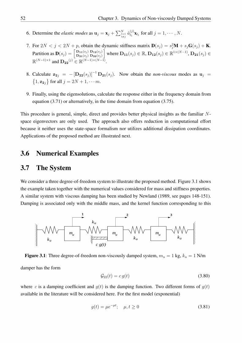
52 Chapter 3. Dynamics of Non-viscously Damped Systems
6. Determine the elastic modes as uj = xj +∑N
l=1l6=j
a(j)l1
xl1 for all j = 1, · · · , N .
7. For 2N < j < 2N + p, obtain the dynamic stiffness matrix D(sj) = s2jM + sjG(sj) + K.
Partition as D(sj) =[
D11(sj) D12(sj)
D21(sj) D22(sj)
]where D11(sj) ∈ R, D12(sj) ∈ R1×(N−1), D21(sj) ∈
R(N−1)×1 and D22(j) ∈ R(N−1)×(N−1).
8. Calculate z2j = − [D22(sj)]−1 D21(sj). Now obtain the non-viscous modes as uj =
1, z2j
for all j = 2N + 1, · · ·m.
9. Finally, using the eigensolutions, calculate the response either in the frequency domain fromequation (3.71) or alternatively, in the time domain from equation (3.75).
This procedure is general, simple, direct and provides better physical insights as the familiar N -space eigenvectors are only used. The approach also offers reduction in computational effortbecause it neither uses the state-space formalism nor utilizes additional dissipation coordinates.Applications of the proposed method are illustrated next.
3.6 Numerical Examples
3.7 The System
We consider a three degree-of-freedom system to illustrate the proposed method. Figure 3.1 showsthe example taken together with the numerical values considered for mass and stiffness properties.A similar system with viscous damping has been studied by Newland (1989, see pages 148-151).Damping is associated only with the middle mass, and the kernel function corresponding to this
u
c g(t)
321
ku
m
ku
m mku ku
u u
Figure 3.1: Three degree-of-freedom non-viscously damped system, mu = 1 kg, ku = 1 N/m
damper has the form
G22(t) = c g(t) (3.80)
where c is a damping coefficient and g(t) is the damping function. Two different forms of g(t)
available in the literature will be considered here. For the first model (exponential)
g(t) = µe−µt; µ, t ≥ 0 (3.81)

3.7. The System 53
and for the second model (double exponential)
g(t) =1
2
(µ1e
−µ1t + µ2e−µ2t
); µ1, µ2, t ≥ 0. (3.82)
The exponential function in (3.81) is possibly the simplest physically realistic non-viscous damp-ing model. This function, often known as a ‘relaxation function’, was introduced by Biot (1955).It has been used extensively in the context of viscoelastic systems. In Chapter 6 a method will beproposed to identify such damping models using modal testing. The double exponential dampingfunction, known as the GHM model, was introduced by Golla and Hughes (1985) and McTavis andHughes (1993). Identification of GHM model has been discussed by Friswell et al. (1997). Bothdamping functions have been scaled so as to have unit area when integrated to infinity. This makesthem directly comparable with the viscous model in which the corresponding damping functionwould be a unit delta function, g(t) = δ(t), and the coefficient c would be the usual viscous damp-ing coefficient. The difference between a delta function and g(t) given by equations (3.81) and(3.82) is that at t = 0 they start with finite values of µ and 1/2 (µ1 + µ2) respectively. Thus, thevalues of µ, µ1 and µ2 give a notion of non-viscousness − if they are large the damping behaviourwill be near-viscous, and vice versa.
The mass and stiffness matrices and the damping matrix in the Laplace domain for the problemcan be obtained as:
M =
mu 0 00 mu 00 0 mu
, (3.83)
K =
2ku −ku 0−ku 2ku −ku
0 −ku 2ku
(3.84)
and
G(s) =
0 0 00 cG(s) 00 0 0
. (3.85)
Here G(s) is the Laplace transform of g(t). Next, the eigensolutions and the dynamic response ofthe system are discussed for the two functional forms of g(t).
3.7.1 Example 1: Exponential Damping
Eigensolutions
We assume c = 0.3, as considered by Newland (1989, page 149) for the equivalent viscouslydamped system. From equation (3.81) one obtains
G(s) =1
s + µ. (3.86)

54 Chapter 3. Dynamics of Non-viscously Damped Systems
Using this expression, the characteristic equation can be simplified as
m3us
7 + m3uµ s6 +
(2 m2
uku + mu (µ cmu + 4 muku))s5 + 6 kum
2uµ s4
+(2 ku (µ cmu + 4 muku) + mu
(2 µ cku + 2 ku
2))
s3 + 10 ku2muµ s2
+ 2 ku
(2 µ cku + 2 ku
2)s + 4 ku
3µ = 0.
(3.87)
The order of the above polynomial, m = 7. Since the system has three degrees of freedom there arethree elastic modes corresponding to the three modes of vibration. The number of the non-viscousmodes, p = m− 2N = 1.
It is of interest to us to understand the effect of ‘non-viscousness’ on the eigensolutions. Figure3.2 shows the locus of the third eigenvalue, that is s3, plotted as a function of µ. It is interesting toobserve that the locus is much more sensitive in the region of lower values of µ (i.e., when dampingis significantly non-viscous) compared to that in the region of higher values. The eigenvalue of thecorresponding viscously damped system is also plotted (marked by *) in the same diagram. Notethat, the non-viscous damping mechanism approaches the viscous damping when µ >≈ 50.0.Similar behaviour has been observed (results not shown here) for the locus of s1 also. The secondmode, in which the middle mass remains stationary, is not effected by damping.
−0.08 −0.07 −0.06 −0.05 −0.04 −0.03 −0.02 −0.01 01.83
1.84
1.85
1.86
1.87
1.88
1.89
1.9
Real
Imag
inar
y
µ=0.601
µ=1.401µ=1.801
µ=3.801
µ=25.0
µ=50.0
viscous damping case
Figure 3.2: Root-locus plot showing the locus of the third eigenvalue (s3) as a function of µ
The eigenvectors of the system, i.e., the three elastic modes (together with their complex con-jugates) and one non-viscous mode can be obtained in a straight forward manner by followingthe steps outlined in the previous section. We select two representative values of µ – one when

3.7. The System 55
µ is large (i.e., near viscous case) and the other when µ is small. The undamped eigenvalues andeigenvectors are obtained as
ω1, ω2, ω3 = 0.7654, 1.4142, 1.8478 (3.88)
and
[x1, x2, x3] =
0.5 0.7071 −0.50.7071 0.0 0.7071
0.5 −0.7071 −0.5
. (3.89)
Using these results, when µ = 50.0, for the elastic modes we have
s1, s2, s3 = −0.0757 + 0.7659i, 1.4142i,−0.0751 + 1.8416i (3.90)
and
[z1, z2, z3] =
0.4983 + 0.0204i 0.7071 −0.5002 + 0.0491i0.7095− 0.0289i 0.0 0.7069 + 0.0694i0.4983 + 0.0204i −0.7071 −0.5002 + 0.0491i
. (3.91)
The above calculation is performed by retaining five terms in the series (3.23). It may be verifiedthat, because µ is large (about 27 times of the maximum natural frequency), the results obtainedare close to the viscously damped case (see Newland, 1989, page 149). For the one non-viscousmode we obtain
s7 = −49.6984 and z7 =
1.02.4719× 103
1.0
(3.92)
Because s7 is purely real and negative this mode is non-oscillatory (over critically damped) andstable.
When µ = 0.5 the damping is significantly non-viscous. For this case, performing similarcalculations for the elastic modes one has
s1, s2, s3 = −0.0207 + 0.8i, 1.4142i,−0.0053 + 1.8671i (3.93)
and
[z1, z2, z3] =
0.4983 + 0.0204i 0.7071 −0.5002 + 0.0491i0.6787 + 0.0112i 0.0 0.7442− 0.0630i0.4983 + 0.0204i −0.7071 −0.5002 + 0.0491i
. (3.94)
These values are not significantly different from those obtained for µ = 50.0 in (3.91). For thisproblem the elastic modes are not very sensitive to the damping mechanism. However, we empha-size that this fact cannot be generalized to all systems. For the non-viscous mode one has
s7 = −0.4480 and z7 =
1.02.2007
1.0
. (3.95)
These values are, however, quite different from those obtained for µ = 50.0 in (3.92). It is difficultto physically visualize the nature of the non-viscous modes in general. These modes are intrinsicto the dampers and we do not have sufficient generalized coordinates to represent them properly.Nevertheless, they yield non-zero residues in the system transfer functions and thus contribute tothe global dynamic response.

56 Chapter 3. Dynamics of Non-viscously Damped Systems
Dynamic Response Analysis
The problem of stationary random vibration analysis of the system is considered here. Supposethe system is subjected to a band-limited Gaussian white noise at the third DOF. We are interestedin the resulting displacement of the system at the third DOF (i.e., z3). The power spectral density(PSD) of the response (see Nigam, 1983, for details) can be given by
Suu(iω) = |H33(iω)|2Sff (iω) (3.96)
where
Sff (iω) =
1 if 0 < ω ≤ 2.5 rad/sec0 otherwise
. (3.97)
In Figure 3.3 the PSD of z3 that is |H33(iω)|2 is plotted for the cases when µ = 50.0 and µ = 0.5.These results are obtained by direct application of equation (3.65). From the diagram observe thatthe damping is less for the case when µ = 0.5 than when µ = 50.0. Also note the (horizontal)shift in the position of the natural frequencies. These features may also be observed in the lootlocus diagram as shown in Figure 3.2. To understand the effect of ‘non-viscosity’, in the samediagram we have plotted the non-viscous term (the second term) appearing in equation (3.65) forboth values of µ. For this problem the non-viscous part is quite small and becomes smaller athigher frequencies. Observe that when µ = 0.5, that is when damping is significantly non-viscous,the value of the non-viscous part of the response is more than that when µ = 50.0. This plot alsoclearly demonstrates that the non-viscous part of the response is not oscillatory in nature.
3.7.2 Example 2: GHM Damping
Taking the Laplace transform of equation (3.82) one obtains
G(s) =(µ1 + µ2) /2 s + µ1µ2
s2 + (µ1 + µ2) s + µ1µ2
. (3.98)
Using this equation, together with the expressions of the system matrices given by equations (3.83)– (3.85), it can be shown that the order of the characteristic polynomial, m = 8. Thus, the numberof the non-viscous modes, p = m−2N = 2. In this section we focus our attention on the numericalaccuracy of the formulation developed in this chapter.
Regarding the numerical values of the damping parameters, we assume c = 0.5, µ1 = 1 andµ2 = 3. Small values of µ1 and µ2 indicate that the damping mechanism is strongly non-viscous.Solving the characteristic equation, exact eigenvalues corresponding to the three elastic modes canbe obtained as
s1, s2, s3 = −0.0994 + 0.8180i, 1.4142i,−0.0687 + 1.9025i (3.99)
and their complex conjugate pairs. Eigenvalues corresponding to the two non-viscous modes arefound to be
s7, s8 = −2.7901,−0.8738. (3.100)

3.7. The System 57
0 0.5 1 1.5 2 2.510
−4
10−3
10−2
10−1
100
101
102
103
104
Frequency (rad/sec)
PS
D
| H33
(i ω)|2, µ = 50.0| H
33(i ω)|2, µ = 0.5
Non−viscous term, µ = 50.0 Non−viscous term, µ = 0.5
Figure 3.3: Power spectral density function of the displacement at the third DOF (z3)
Eigenvalues corresponding to the elastic modes can also be obtained approximately by equation(3.33) in Section 3.2.3. Recall that only the undamped eigensolutions are required in order to applythis equation. Approximate eigenvalues using equation (3.33) are calculated as
s1, s2, s3approx = −0.0981− 0.8105i, 1.4142i,−0.0595− 1.9018i. (3.101)
It is useful to compare the exact and approximate eigenvalues in the light of the Q-factors. In thisproblem the second mode is not damped, so Q2 = ∞. For the first and third modes we obtainQ1 = 4.1164 and Q3 = 13.8540. Small values of Q-factor indicate that these modes are quiteheavily damped. Comparing equations (3.99) and (3.101) it may be observed that the approximatevalues are quite close to the exact one even when damping is reasonably high.
In order to check the numerical accuracy of the eigenvectors, first the exact values are calculatedby the matrix inversion method. For the elastic modes we obtain
[z1, z2, z3] =
0.5114 + 0.0299i 0.7071 −0.4639 + 0.0403i0.6905− 0.0431i 0.0 0.7596 + 0.0562i0.5114 + 0.0299i −0.7071 −0.4639 + 0.0403i
(3.102)
and their complex conjugates. For the two non-viscous modes one has
[z7, z8] =
1.0000 1.00009.7847 2.76361.0000 1.0000
. (3.103)

58 Chapter 3. Dynamics of Non-viscously Damped Systems
Approximate eigenvectors corresponding to the elastic modes, calculated by equation (3.35), areobtained as
[z1, z2, z3]approx =
0.5114 + 0.0299i 0.7071 −0.4639 + 0.0403i0.6910− 0.0422i 0.0 0.7582 + 0.0569i0.5114 + 0.0299i −0.7071 −0.4639 + 0.0403i
. (3.104)
The above values are equivalent to performing the calculation by retaining only one term in theseries (3.23). Also recall that the approximate values are obtained from the undamped eigensolu-tions only. Comparing equation (3.102) and (3.104) it is clear that the results obtained from theapproximate method match the exact solutions to an excellent accuracy.
As a final check on the formulation developed in this chapter, we compare the transfer func-tion obtained from equation (3.65) with the exact transfer function calculated by inversion of thedynamic stiffness matrix. Figure 3.4 shows such a comparison for H33(iω). Approximate naturalfrequencies and modes given by (3.101) and (3.104) are used and also the non-viscous term inequation (3.65) is neglected in order to calculate the approximate transfer function. Thus, in turn,the approximate transfer function in Figure 3.4 is obtained only by proper ‘post-processing’ of theundamped eigensolutions. From this figure it may be observed that, except in a few places, theapproximate transfer function is reasonably close to the exact one. This analysis demonstrates theusefulness of the proposed method.
0 0.5 1 1.5 2 2.510
−1
100
101
102
Frequency (rad/sec)
| H33
(i ω)
|
Exact, by matrix inversion Approximate, by series expansion
Figure 3.4: Transfer function H33(iω)

3.8. Conclusions 59
3.8 Conclusions
The problem of dynamic analysis of non-viscously damped multiple-degrees-of-freedom linearsystems has been considered. The assumed non-viscous damping model is such that the dampingforces depend on the past history of motion via convolution integrals over some kernel functions.It has been assumed that, in general, the mass and stiffness matrices as well as the matrix of thekernel functions cannot be simultaneously diagonalized by any linear transformation. The analysisis, however, restricted to systems with non-repetitive eigenvalues and non-singular mass matrices.
The system eigenvalues were obtained by solving the characteristic equation. It turns out that,unlike viscously damped systems, the order of the characteristic equation for an N -degrees-of-freedom system is more than 2N . As a consequence, the number of modes become more than2N and they were grouped into two types – (a) elastic modes and (b) non-viscous modes. It isassumed that the elastic modes appear in complex conjugate pairs, that is, they are sub-criticallydamped. The elastic modes, which consist of N eigenvectors together with their complex conju-gate pairs, correspond to N modes of vibration of the structural system. These N eigenvectorswere expressed as a complex linear combination of the (real) eigenvectors of the correspondingundamped system. The vector of these complex constants were further determined from a seriesobtained by the Neumann expansion method. Based on this analysis, some approximate formulasfor the eigenvalues and eigenvectors were suggested and their accuracy were verified using numer-ical examples. The non-viscous modes, which occur due to the non-viscous damping mechanism,are real, over critically damped and non-oscillatory in nature. These modes were obtained byinversion of a partition of the dynamic stiffness matrix evaluated at the corresponding eigenvalues.
The transfer function matrix of the system was derived in terms of the eigenvalues and eigen-vectors of the second-order system. Exact closed-form expressions of the response due to arbitraryforcing functions and initial conditions were obtained. The response can be expressed as a sumof two parts, one that arises in usual viscously damped systems and the other that occurs due tonon-viscous damping mechanisms. Through an example it was shown that the non-viscous part ofthe response is purely dissipative and non-oscillatory in nature.
The method developed here is analogous to classical modal analysis where undamped naturalfrequencies and modes have to be appropriately replaced by elastic modes and non-viscous modesof the non-conservative system. The method presented offers a reduction in computational effortbecause neither the first-order formalisms nor the additional dissipation coordinates are employed.Moreover, this approach also provides better physical insight as familiar N -space eigenvectors areutilized.

60 Chapter 3. Dynamics of Non-viscously Damped Systems

Chapter 4
Some General Properties of theEigenvectors
4.1 Introduction
In the last chapter, the eigenvalues, eigenvectors and transfer functions associated with multiple-degrees-of-freedom non-viscously damped systems have been discussed. A method was outlinedto obtain the eigenvectors and dynamic response of the system. Although the method is analogousto classical modal analysis, unlike the classical modes, very little is known about qualitative prop-erties of the modes of non-viscously damped systems. Purpose of this chapter is to develop somebasic relationships satisfied by the eigensolutions and the system matrices of (3.1). Specifically wehave focused our attention to the normalization and orthogonality relationship of the eigenvectors.
4.2 Nature of the Eigensolutions
The eigenvalue problem associated with equation (3.1) can be defined as
[s2
jM + sj G(sj) + K]
zj = 0 or D(sj)zj = 0, ∀ k = 1, · · · ,m (4.1)
where the dynamic stiffness matrix
D(s) = s2M + s G(s) + K ∈ CN×N . (4.2)
Here zj is the j-th eigenvector and sj is the j-th eigenvalue. In general the number of eigenvalues,m = 2N + p; p ≥ 0. It is assumed that all m eigenvalues are distinct. It should be noted thateigenvalue problems of this kind are not similar to the eigenvalue problems arise in the contextof Lambda-matrices (Lancaster, 1966) because G(s) is not a constant matrix. We consider thedamping to be ‘non-proportional’, that is, the mass and stiffness matrices as well as the matrixof the kernel functions cannot be simultaneously diagonalized by any linear transformation. It isassumed that |Gjk(s)| < ∞ when s → ∞. This in turn implies that the elements of G(s) are at
61

62 Chapter 4. Some General Properties of the Eigenvectors
the most of order 1/s in s or constant, as in the case of viscous damping. Construct the diagonalmatrix containing the eigenvalues as
S = diag [s1, s2, · · · , sm] ∈ Cm×m (4.3)
and the matrix containing the eigenvectors (the modal matrix) as
Z = [z1, z2, · · · , zm] ∈ CN×m. (4.4)
Next, we consider the normalization relationship of the eigenvectors.
4.3 Normalization of the Eigenvectors
Premultiplying equation (4.1) by zTk , applying equation (4.1) for k-th set and postmultiplying by
zj and subtracting one from the other we obtain
zTk
[(s2
j − s2k
)M + sjG(sj)− skG(sk)
]zj = 0. (4.5)
Since sj and sk are distinct for different j and k, the above equation can be divided by (sj − sk) toobtain
zTk
[(sj + sk) M +
sjG(sj)− skG(sk)
sj − sk
]zj = 0, ∀j, k; j 6= k. (4.6)
This equation may be regarded as the orthogonality relationship of the eigenvectors. It is easyto verify that, in the undamped limit equation (4.6) degenerates to the familiar mass orthogonal-ity relationship of the undamped eigenvectors. However, this orthogonality relationship is not veryuseful because it is expressed in terms of the natural frequencies. A frequency-independent orthog-onality relationship of the eigenvectors will be derived later in this chapter. Assuming δs = sj−sk,rewrite equation (4.6) as
zTk
[(δs + 2sk) M +
(sk + δs) G(sk + δs)− skG(sk)
δs
]zj = 0. (4.7)
Consider the case when sj → sk, that is, δs → 0. For this limiting case, equation (4.7) reads
zTk
[2skM +
∂ [sG(s)]
∂s|sk
]zk = θk (4.8)
or zTk [2skM + G(sk) + skG′(sk)] zk = θk, (4.9)
∀k = 1, · · · ,m
for some non-zero θk ∈ C. Equation (4.9) is the normalization relationship for the eigenvectorsof the non-viscously damped system (3.1). From the expression of the dynamic stiffness matrix in(4.2), the normalization condition in equation (4.9) can also be expressed as
zTk D′(sk)zk = θk, ∀k = 1, · · · ,m. (4.10)

4.4. Orthogonality of the Eigenvectors 63
Equation (4.9), and consequently equation (4.10), can be regarded as the generalization of the‘mass normalization’ relationship used in structural dynamics. In the undamped limit when G(s)
is a null matrix, equation (4.9) reduces to the familiar mass normalization relationship for theundamped eigenvectors. For viscously damped systems (see Section 4.7 for details), relationshipanalogous to (4.9) was obtained, for example, by Sestieri and Ibrahim (1994) using state-spaceapproach and, by Fawzy and Bishop (1976) and Fawzy (1977) using second-order equations ofmotion. We define the normalization matrix, Θ, as
Θ = diag [θ1, θ2, · · · , θm] ∈ Cm×m. (4.11)
Numerical values of θk can be selected in various ways:
• Choose θk = 2sk, ∀k that is Θ = 2S. This reduces to zTk Mzk = 1, ∀k when the damping is
zero. This is consistent with the unity modal mass convention, often used in experimentalmodal analysis and finite element methods.
• Choose θk = 1 + 0i,∀k, that is, Θ = Im. Theoretical analysis becomes easiest with thisnormalization. However, as pointed out by Fawzy (1977) and Vigneron (1986) in the contextof viscously damped systems, this normalization is inconsistent with undamped or classicallydamped modal theories.
4.4 Orthogonality of the Eigenvectors
The orthogonality relationship of the eigenvectors given by equation (4.6) is not very useful be-cause it is expressed in terms of the eigenvalues of the system. In this section, we will develop anorthogonality relationship which is independent of the eigenvalues. Expressions equivalent to theorthogonality relationships of the undamped eigenvectors with respect to the mass and stiffnessmatrices will also be established. In order to derive these results, first recall the expression of thetransfer function matrix derived in Section 3.3. In the pole-residue form the inverse of the dynamicstiffness matrix (transfer function matrix) can be expressed as
D−1(s) =adj [D(s)]
det [D(s)]=
m∑j=1
Rj
s− sj
. (4.12)
Here Rj , the residue of D−1(s) at the pole sj obtained from equation (3.64) as
Rj =zjzT
j
zTj
∂D(sj)
∂sjzj
∈ CN×N . (4.13)
Interestingly, observe that denominator of left-hand side of the above equation is exactly the sameas the normalization condition given by equation (4.10). Now, using equations (4.10) and (4.13)one finally obtains the residues as
Rj =zjzT
j
θj
. (4.14)

64 Chapter 4. Some General Properties of the Eigenvectors
For undamped systems, i.e., when G(s) = ON , ∀ s, the eigenvectors satisfy familiar orthog-onality relationship over the mass and stiffness matrices as given by equations (1.10) and (1.11).For viscously damped systems (with non-proportional damping), equivalent relationships may beobtained by converting the equations of motion into the state-space form (see Sestieri and Ibrahim,1994). The eigenproblem in the state-space form is essentially similar to the undamped eigen-problem except that the size of the problem gets doubled, and the eigensolutions become complex.Thus, from the analysis point of view, the state-space approach offers significant advantage forviscously damped systems. Unfortunately, for non-viscously damped systems, no advantage canbe gained by adopting the state-space formalism as at least one of the system matrices will not be aconstant matrix. For this reason, and also realizing that the state-space eigenvectors are not phys-ically appealing, we kept the analysis in the second-order form. One of our main result regardingthe orthogonality of the eigenvectors is the following:Theorem 4.1. The modal matrix of a non-viscously damped system, Z ∈ CN×m, satisfy the or-
thogonality relationship ZΘ−1ZT = ON .
Proof. From equations (4.12) and (4.14) one obtains
adj [D(s)]
det [D(s)]=
m∑j=1
1
s− sj
zjzTj
θj
. (4.15)
Multiplying both side of the above equation by s and taking limit as s →∞ we obtain
lims→∞
sadj [D(s)]
det [D(s)]= lim
s→∞
m∑j=1
s
s− sj
zjzTj
θj
=m∑
j=1
zjzTj
θj
. (4.16)
It is easy to observe that the order of the elements of adj [D(s)] is at the most (m− 2) in s. Sincethe order of the determinant, det [D(s)], is m, after taking the limit every element of the left-handside of equation (4.16) reduces to zero. Thus, in the limit, the left-hand side of equation (4.16)approaches to an N ×N null matrix. Finally, writing equation (4.16) in the matrix form we obtain
ZΘ−1ZT = ON (4.17)
and the theorem is proved.
The result of this theorem is quite general and it does not depend on the nature of the systemproperty matrices. The only requirement of this theorem is that the system must have m ≥ 2N dis-tinct eigenvalues. Clearly, the undamped systems as well as the viscously damped systems are alsocovered as special cases. In the context of viscously damped systems (see Section 4.7 for details),similar result has been derived by Fawzy and Bishop (1976) by considering the normalization ma-trix Θ as the identity matrix. Later Fawzy (1977) generalized this result for the case when Θ is notan identity matrix. The result obtained in theorem 4.1 can be viewed as a further generalization ofthese results to the non-viscously damped systems. Next, we consider the relationship between theeigensolutions and the mass matrix.

4.4. Orthogonality of the Eigenvectors 65
Theorem 4.2. The modal matrix of a non-viscously damped system, Z ∈ CN×m, satisfy the rela-
tionship ZΘ−1SZT = M−1.
Proof. First consider the function sD−1(s). Following the approach outlined in Section 3.3.2 andusing the residue theorem one obtains
sD−1(s) =m∑
j=1
Qj
s− sj
. (4.18)
Here the residues Qj can be obtained as
Qjdef= lim
s→sj
(s− sj)[sD−1(s)
]= sj
zjzTj
θj
. (4.19)
Using the expression of the dynamic stiffness matrix in equation (4.2) we can deduce
lims→∞
D(s)
s2= lim
s→∞
[M +
G(s)
s+
Ks2
]= M. (4.20)
Taking the inverse of the above equation results
lims→∞
[s2D−1(s)
]= M−1. (4.21)
Now, multiplying equation (4.18) by s and taking limit as s →∞ we obtain
lims→∞
[s2D−1(s)
]= lim
s→∞
m∑j=1
s
s− sj
sjzjzTj
θj
=m∑
j=1
sjzjzTj
θj
. (4.22)
Casting the right-hand side of the above equation in the matrix form and equating it with (4.21)results
ZΘ−1SZT = M−1 (4.23)
and the theorem is proved.
Since Θ and S are diagonal matrices, they commute in product. For this reason the aboveresult can also be expressed as ZSΘ−1ZT = M−1. For viscously damped systems, similar resulthas been derived by Fawzy and Bishop (1976) by considering the normalization matrix Θ as theidentity matrix. It might be thought that by taking the inverse of equation (4.23) and rearranging,the conventional mass-orthogonality relationship
ZT MZ = S−1Θ (4.24)
could be obtained. We emphasize that the representation of equation (4.23) in the form of equation(4.24) is not always possible. To show this, premultiply equation (4.24) by ZΘ−1 to obtain
ZΘ−1ZT MZ = ZΘ−1S−1Θ = ZS−1. (4.25)

66 Chapter 4. Some General Properties of the Eigenvectors
Due to theorem 4.1, the left-hand side of equation (4.25) is a null matrix, while its right-hand sideis not. Thus (4.24) cannot be a valid equation. However, for a special case, when the system isundamped, the modal matrix Z can be expressed by a square matrix and equation (4.23) can berepresented by the classical mass-orthogonality relationship in (4.24). Thus, theorem 4.2 providesthe result equivalent to the classical mass-orthogonality relationship for general cases.
Like the mass-orthogonality relationship of the eigenvectors, the orthogonality relationshipwith respect to the stiffness matrix can also be obtained. Assuming that K−1 exists we have thefollowing:Theorem 4.3. The modal matrix of a non-viscously damped system, Z ∈ CN×m, satisfy the rela-
tionship ZΘ−1S−1ZT = −K−1.
Proof. Using the expression of the dynamic stiffness matrix in equation (4.2) we can easily deduce
lims→0
D(s) = K. (4.26)
Taking the inverse of the above equation results
lims→0
D−1(s) = K−1. (4.27)
From equations (4.12) and (4.14) one obtains
D−1(s) =m∑
j=1
1
s− sj
zjzTj
θj
. (4.28)
Taking the limit as s → 0 in equation (4.28) we obtain
lims→0
D−1(s) =m∑
j=1
1
−sj
zjzTj
θj
. (4.29)
Casting the right-hand side of the preceding equation in the matrix form and equating it with (4.27)results
ZΘ−1S−1ZT = −K−1 (4.30)
and the theorem is proved.
4.5 Relationships Between the Eigensolutions and Damping
In the last section, some direct relationships have been established between the mass and stiffnessmatrices and the eigensolutions. In this section we try to establish the relationships between thedamping matrix and the eigensolutions. A major difficulty in this regard is that, unlike the massand stiffness matrices, the damping matrix, G(s), is a function of s. To simplify the problem weconsider only two limiting cases, (a) when s →∞, and (b) when s → 0. Suppose
lims→∞
G(s) = G∞ ∈ RN×N (4.31)
and lims→0
G(s) = G0 ∈ RN×N , (4.32)
where ‖G∞‖, ‖G0‖ < ∞.

4.5. Relationships Between the Eigensolutions and Damping 67
4.5.1 Relationships in Terms of M−1
Casting equation (4.28) into the matrix form one obtains
D−1(s) = ZΘ−1 (sIm − S)−1 ZT . (4.33)
The preceding equation can be expanded as
D−1(s) =1
sZΘ−1
(Im − S
s
)−1
ZT
=1
s
(ZΘ−1ZT
)+
1
s2
(ZΘ−1SZT
)
+1
s3
(ZΘ−1S2ZT
)+
1
s4
(ZΘ−1S3ZT
)+ · · ·
(4.34)
Now, rewrite the expression of the dynamic stiffness matrix in equation (4.2) as
D(s) = s2M[
IN +M−1
s
(G(s) +
Ks
)]. (4.35)
Taking the inverse of this equation and expanding the right-hand side one obtains
D−1(s) =
[IN − M−1
s
(G(s) +
Ks
)
+
M−1
s
(G(s) +
Ks
)2
− · · ·]
M−1
s2.
(4.36)
Equation (4.36) can be further simplified to obtain
D−1(s) =M−1
s2+
1
s3
(−M−1G(s)M−1)
+1
s4
(M−1
[G(s)M−1G(s)−K
]M−1
)+ · · ·
(4.37)
Comparing equations (4.34) and (4.37) it is clear that their right-hand sides are equal. Theorems1 and 2 can be alternatively proved by multiplying these equations by s and s2 respectively andtaking the limit as s → ∞. Observe that, the coefficients associated with the corresponding(negative) powers of s in the series expressions (4.34) and (4.37) cannot be equated because G(s)
is also a function of s. However, in the limit when s → ∞, the variation of G(s) becomesnegligible as by equation (4.31) it approaches to G∞. Considering the second term of the right-hand side of equation (4.37), equating it with the corresponding term of equation (4.34) and takingthe limit as s →∞ one obtains
ZΘ−1S2ZT = −M−1G∞M−1. (4.38)
It must be noted that this procedure cannot be extended to further lower order terms as all of themwould be effected by the functional variation of G(s) from previous terms.
Were the system viscously damped G(s) would be a constant matrix and equating the coef-ficients associated with different powers of s one could obtain several relationships between theeigensolutions and the system matrices. Considering the first few terms in the series expressions(4.34) and (4.37), some such relationships are reported in Section 4.7.

68 Chapter 4. Some General Properties of the Eigenvectors
4.5.2 Relationships in Terms of K−1
We rewrite equation (4.33) as
D−1(s) = −ZΘ−1S−1(Im − sS−1
)−1 ZT . (4.39)
Expanding equation (4.39) one obtains
D−1(s) =− ZΘ−1S−1ZT − s(ZΘ−1S−2ZT
)
− s2(ZΘ−1S−3ZT
)− s3(ZΘ−1S−4ZT
)− · · ·(4.40)
The expression of the dynamic stiffness matrix in equation (4.2) can be rearranged as
D(s) = K[IN + s
(sK−1M + K−1G(s)
)]. (4.41)
Taking the inverse of equation (4.41) and expanding the right-hand side one obtains
D−1(s) =[IN − s
(sK−1M + K−1G(s)
)
+s(sK−1M + K−1G(s)
)2 − · · ·]
K−1.(4.42)
The preceding equation can be further simplified to obtain
D−1(s) =K−1 + s(−K−1G(s)K−1
)
+ s2(K−1
[G(s)K−1G(s)−M
]K−1
)+ · · ·
(4.43)
Comparing the right-hand side of equations (4.40) and (4.43), theorem 4.3 can be proved alterna-tively by taking the limit as s → 0. Considering the second term of the right-hand side of equation(4.43), equating it with the second term of equation (4.40) and taking the limit as s → 0 oneobtains
ZΘ−1S−2ZT = K−1G0K−1. (4.44)
Again, note that this approach cannot be extended to the higher order terms as all of them wouldbe effected by the functional variation of G(s) from previous terms.
4.6 System Matrices in Terms of the Eigensolutions
Theorems 4.2, 4.3 and equations (4.38), (4.44) allow us to represent the system property matricesexplicitly in terms of the eigensolutions. This might be useful in system identification problemswhere the eigensolutions of a structure can be measured from experiments. Using the eigensolu-tions we define two matrices
P1 = ZΘ−1SZT (4.45)
and P2 = ZΘ−1S−1ZT . (4.46)

4.7. Eigenrelations for Viscously Damped Systems 69
Using these equations, from equation (4.23) one obtains the mass matrix as
M = P−11 . (4.47)
Similarly from equation (4.30) the stiffness matrix can be obtained as
K = −P−12 . (4.48)
The damping matrix in the Laplace domain, G(s), can be obtained only at the two limiting valueswhen s →∞, and s → 0. From equations (4.38) and (4.44) one obtains
G∞ = −P−11
[ZΘ−1S2ZT
]P−1
1 (4.49)
and G0 = P−12
[ZΘ−1S−2ZT
]P−1
2 . (4.50)
These results, however, do not give any indication regarding the functional behaviour of G(s)
between these two extreme values.
4.7 Eigenrelations for Viscously Damped Systems
Viscously damped systems arise as a special case of the more general non-viscously damped sys-tems when the damping matrix become a constant matrix, that is, G(s) = C ∈ RN×N ,∀ s. Here,several relationships satisfied by the eigensolutions and the system matrices will be derived for thisspecial case.
For viscously damped systems the order of the characteristic polynomial m = 2N , and conse-quently the modal matrix Z ∈ CN×2N and the diagonal matrices S,Θ ∈ C2N×2N . From equation(4.9), the normalization relationship reads
zTk [2skM + C] zk = θk, ∀k = 1, · · · , 2N. (4.51)
Now, consider the series expansion of D−1(s) given by equations (4.34) and (4.37). Equating thecoefficients of 1/s we obtain the mode orthogonality relationship
ZΘ−1ZT = ON . (4.52)
This relationship was also derived by Fawzy (1977). Now, equating the coefficients of 1/s2, · · · , 1/s5
in the right hand sides of equations (4.34) and (4.37), several relationships involving the eigenso-lutions and M−1, C and K may be obtained:
ZΘ−1SZT = M−1 (4.53)
ZΘ−1S2ZT = −M−1CM−1 (4.54)
ZΘ−1S3ZT = M−1[CM−1C−K
]M−1 (4.55)

70 Chapter 4. Some General Properties of the Eigenvectors
andZΘ−1S4ZT = M−1
[KM−1C + CM−1K− CM−1CM−1C
]M−1. (4.56)
This procedure can be extended to obtain further higher order terms involving S.Similarly, equating the coefficients of s0, · · · , s3 in the right-hand sides of equations (4.40) and
(4.43), several relationships involving the eigensolutions and K−1, C and M may be obtained:
ZΘ−1S−1ZT = −K−1 (4.57)
ZΘ−1S−2ZT = K−1CK−1 (4.58)
ZΘ−1S−3ZT = K−1[M− CK−1C
]K−1 (4.59)
andZΘ−1S−4ZT = K−1
[CK−1CK−1C−MK−1C + CK−1M
]K−1. (4.60)
This procedure can be extended to obtain further lower order terms involving S. Employing adifferent approach, and considering the normalization matrix Θ as the identity matrix, Fawzy andBishop (1976) obtained expressions similar to equations (4.53) – (4.55) and (4.57) – (4.59). Thus,the relationships derived here extend their results to generally normalized eigenvectors.
4.8 Numerical Examples
4.8.1 The System
A three-degree-of-freedom system, similar to what considered in Section 3.7, is used to illustratethe results derived in this chapter. The mass and stiffness matrices are assumed to be
M =
3 0 00 3 00 0 3
(4.61)
and K =
4 −2 0−2 4 −2
0 −2 4
. (4.62)
Numerical values for these matrices are taken by assuming mu = 3 and ku = 2 in the exampleconsidered in Section 3.7. The matrix of the damping functions is assumed to be of the form
G(t) =
0 0 00 1.5g(t) 00 0 0
(4.63)
whereg(t) = δ(t) +
(µ1e
−µ1t + µ2e−µ2t
); µ1, µ2 > 0. (4.64)
The damping matrix in the Laplace domain, G(s), can be obtained by taking the Laplace transformof equation (4.63). The Laplace transform of g(t) given by (4.64) can be obtained as
G(s) = 1 +(µ1 + µ2) s + 2µ1µ2
s2 + (µ1 + µ2) s + µ1µ2
. (4.65)

4.8. Numerical Examples 71
This damping model is a linear combination of the viscous model and the GHM model consideredin the last chapter. Regarding the numerical values of the damping parameters, we assume µ1 = 1.5
and µ2 = 0.1.
4.8.2 Eigenvalues and Eigenvectors
Using equation (4.65), together with the expressions of the system matrices given by equations(4.61) – (4.63), it can be shown that the order of the characteristic polynomial, m = 8. It hasbeen mentioned that (for lightly damped systems), among the m eigenvalues, 2N = 6 appear incomplex conjugate pairs (elastic modes) and the rest p = m− 2N = 2 eigenvalues become purelyreal (non-viscous modes).
Solving the characteristic equation, the diagonal matrix containing the eigenvalues can be ex-pressed as
S = diag [se, s∗e, sn] ∈ C8×8. (4.66)
Here, the eigenvalues corresponding to the three elastic modes are
se = −0.2632 + 0.7363i, 1.1547i,−0.2392 + 1.5177i, . (4.67)
The eigenvalues corresponding to the two non-viscous modes are found to be
sn = −1.0029,−0.0921 . (4.68)
Since these eigenvalues are purely real and negative, it implies that the non-viscous modes arestable and non-oscillatory in nature (i.e., over critically damped).
The eigenvectors can be obtained by applying the procedure outlined in the last chapter. Thematrix of eigenvectors can be expressed as
Z = [Ze, Z∗e, Zn] ∈ C3×8 (4.69)
Here, Ze, the matrix of eigenvectors corresponding to the three elastic modes, is
Ze =
1 1 11.2908− 0.5814i 0 −1.3690− 1.0893i
1 −1 1
. (4.70)
The matrix of eigenvectors corresponding to the two non-viscous modes is calculated as
Zn =
1 13.5088 2.0127
1 1
. (4.71)
Using the eigenvectors given by equations (4.70) – (4.71), the normalization matrix Θ can beobtained from equation (4.9) as
Θ = diag [θe,θ∗e,θn] . (4.72)

72 Chapter 4. Some General Properties of the Eigenvectors
Here
θe = 0.0223 + 0.1180i, 0.1386i,−0.2756 + 0.2359i (4.73)
and
θn = 1.0075, 9.8738 . (4.74)
4.8.3 Orthogonality Relationships
Using Z and Θ one can easily verify that the mode orthogonality relationship given by theorem4.1 is satisfied, that is,
ZΘ−1ZT = O3. (4.75)
Now, in the line of theorem 4.2 we calculate
ZΘ−1SZT =
0.3333 0 00 0.3333 00 0 0.3333
= M−1. (4.76)
Similarly, following theorem 4.3 one obtains
− ZΘ−1S−1ZT =
0.375 0.250 0.1250.250 0.500 0.2500.125 0.250 0.375
= K−1. (4.77)
4.8.4 Relationships With the Damping Matrix
Taking the Laplace transform of equation (4.63) and considering the limiting cases as s →∞, ands → 0 one obtains
G∞ =
0 0 00 1.5 00 0 0
(4.78)
and G0 =
0 0 00 4.5 00 0 0
. (4.79)
Note that the matrices P1 and P2, defined in equations (4.45) and (4.46) respectively, can be directlyobtained from (4.76) and (4.77). Using these matrices, the truth of equations (4.49) and (4.50),which relate G∞ and G0 to the eigensolutions, can be verified. Thus, the damping matrix, G(s),can be reconstructed from the eigensolutions for the cases when s →∞, and s → 0.
4.9 Conclusions
In this chapter we have developed several eigenrelations for non-viscously damped multiple-degrees-of-freedom linear dynamic systems. It has been assumed that, in general, the mass and

4.9. Conclusions 73
stiffness matrices as well as the matrix of the kernel functions cannot be simultaneously diago-nalized by any linear transformation. The analysis is, however, restricted to systems with non-repetitive eigenvalues and non-singular mass matrices. Relationships regarding the normalizationand the orthogonality of the (complex) eigenvectors have been established (theorem 4.1). Expres-sions equivalent to the orthogonality of the undamped modes over the mass and stiffness matriceshave been proposed (theorems 4.2 and 4.3). It was shown that the classical relationships can beobtained as special cases of these general results. Based on these results, we have shown that themass and stiffness matrices can be uniquely expressed in terms of the eigensolutions. The damp-ing matrix, G(s), cannot be reconstructed using this approach because it is not a constant matrix.However, we have provided expressions which relate the damping matrix to the eigensolutions forthe cases when s → ∞, and s → 0. Whenever applicable, viscously damped counterparts of thenewly developed results were provided.

74 Chapter 4. Some General Properties of the Eigenvectors

Chapter 5
Identification of Viscous Damping
5.1 Introduction
In Chapters 3 and 4, a systematic study on modal analysis of generally damped linear systems hasbeen carried out. The results based on these studies give a firm basis for further analysis, to use thedetails of the measured vibration data to learn more about the underlying damping mechanisms.It was shown that non-viscously damped systems have two types of modes, (a) elastic modes,and (b) non-viscous modes. The elastic modes correspond to the ‘modes of vibration’ of a linearsystem. The non-viscous modes occur due to the non-viscous damping mechanism and they are notoscillatory in nature. For an underdamped system, that is a system whose all modes are vibrating,the elastic modes are complex (appear in complex conjugate pairs) and non-viscous modes are real.For an N -degrees-of-freedom non-viscously damped systems there are exactly N pairs of elasticmodes. The number of non-viscous modes depends on the nature of the damping mechanisms.Conventional viscously damped systems are special cases of non-viscously damped systems whenthe damping kernel functions have no ‘memory’. Modes of viscously damped systems consist ofonly (complex) elastic modes as non-viscous modes do not appear in such systems. Elastic modescan be real only if the damping is proportional, that is only if the conditions derived in Theorem2.2 are satisfied.
There is no physical reason why a general system should follow the mathematical conditionsfor existence of real normal modes. In fact practical experience in modal testing shows that mostreal-life structures do not do so, as they possess complex modes instead of real normal modes.As Sestieri and Ibrahim (1994) have put it ‘ ... it is ironic that the real modes are in fact not realat all, in that in practice they do not exist, while complex modes are those practically identifiablefrom experimental tests. This implies that real modes are pure abstraction, in contrast with complexmodes that are, therefore, the only reality!’ For this reason it is legitimate to consider only complexmodes for further developments. However, consideration of complex modes in experimental modalanalysis has not been very popular among researchers. In fact many publications, for exampleIbrahim (1983a), Chen et al. (1996b) and Balmes (1997), discuss how to obtain the ‘best’ realnormal modes from identified complex modes.
75

76 Chapter 5. Identification of Viscous Damping
The works in the previous chapters made it clear that the standard procedure of experimentalmodal analysis actually measured ‘modes’ when complex results were obtained. The justificationof the method in the standard texts (eg., Ewins, 1984) is based on assuming viscous damping, andbegs the question of how one might tell in practice whether a viscous model is applicable to agiven structure, let alone of how to proceed if a viscous model is not supported by the measure-ments. These are the central questions to be addressed in this study. The works in the earlierchapters showed that the expression for vibration transfer functions in terms of mode shapes andnatural frequencies, familiar from undamped systems, carries over almost unchanged to systemswith completely general linear damping. One simply replaces the mode shapes with correspondingcomplex elastic modes and non-viscous modes, and the natural frequencies with their correspond-ing values. This result shows that experimental modal analysis can indeed measure the correctcomplex modes of a structure, since the pole-fitting strategy normally used is based on the validityof this transfer function expression. Here we emphasize that by conducting conventional modaltesting procedure it is only possible to obtain the elastic modes as the non-viscous modes do notproduce any ‘peak’ in the measured transfer functions (see Section 8.2 for further discussions ).This is however, not a very big limitation since it was shown before that the effect of non-viscousmodes is not very significant on the vibration response. For this reason, in what follows next, thenon-viscous modes will not be considered. Beside this we also assume that the damping is light sothat the first-order perturbation method can be applied.
There are good arguments to support the principle of reciprocity when the physical mechanismof damping arises from linear viscoelastic behaviour within some or all of the material of which thestructure is built. The ‘correspondence principle’ of linear viscoelasticity applies to such problemsunder rather general conditions (see eg., Fung, 1965), and since the undamped problem satisfiesreciprocity, then the damped one will also do so. However, the case is less obvious for dampingassociated with structural joints, often the dominant source of damping in practice. The mech-anisms of such damping are frequently non-linear when examined in detail, but empirically theoverall result frequently satisfies normal experimental tests of linearity. The question of whethersuch systems should be expected to satisfy reciprocity remains open. For the purpose of the presentinvestigation, reciprocity will be assumed in all cases.
These facts gives us the confidence to ask some general questions of interest:
1. From experimentally determined complex modes can one identify the underlying dampingmechanism? Is it viscous or non-viscous? Can the correct model parameters be found ex-perimentally?
2. Is it possible to establish experimentally the spatial distribution of damping?
3. Is it possible that more than one damping model with corresponding ‘correct’ sets of param-eters may represent the system response equally well, so that the identified model becomesnon-unique?

5.2. Background of Complex Modes 77
4. Does the selection of damping model matter from an engineering point of view? Whichaspects of behaviour are wrongly predicted by an incorrect damping model?
This chapter and following two address these questions. The analysis is restricted to linear systemswith light damping: we assume throughout the validity of the first-order perturbation results. Theinitial aim is to consider what can be learned about these questions in principle, so procedures willbe illustrated by applying them to simulated transfer functions, with no noise. The issue of how theusefulness of any procedure might be limited in practice by measurement noise will be deferred tolater studies. This chapter will concentrate on the fitting of viscous models to ‘measured’ transferfunctions, and on establishing the symptoms by which a non-viscous model might be recognized.In Section 5.2 we briefly review the theory of determination of complex frequencies and modesbased on the first-order perturbation method. In Section 5.3 an algorithm is given for fitting anon-proportional viscous damping model, using the complex modes and complex frequencies. InSection 5.4 numerical examples are given to illustrate the fitting procedure. Some implications ofthese results for damping identification are summarized in Section 5.5. In Chapter 6, the proceduresare generalized to some non-viscous models of damping, and the discussion extended to this moregeneral case.
5.2 Background of Complex Modes
Dynamics of viscously damped systems has been discussed in details in Section 1.3. Complexmodes arise in viscously damped systems provided the damping is non-proportional. Expressionsof complex modes can be obtained as a special case of the general analysis presented in Section3.2.1. One such special case when the damping is lightly non-proportional is discussed in Section3.2.3. In this section we consider a further special case when the damping is light so that the first-order perturbation method can be applied. First-order perturbation results can be obtained fromthe results in Section 3.2.3 as follows.
Suppose λj, zj is the j-th complex natural frequency and complex mode shape. In the contextof the notations used in Section 3.2.3, sj = iλj . Using this, from equation (3.37) approximateexpression for the complex natural frequencies can be obtained as
λj ≈ ±ωj + iC ′jj/2. (5.1)
From equation (3.38), the first-order approximate expression of the complex eigenvectors is
zj ≈ xj + iN∑
k=1k 6=j
ωjC′kj
(ω2j − ω2
k)xk. (5.2)
In the above expressions C ′kl = xT
k Cxl are the elements of the damping matrix in modal coordi-nates. These results were obtained by Rayleigh (1877, see Section 102, equation 5 and 6). The

78 Chapter 5. Identification of Viscous Damping
above equation shows (up to first order approximation) that the real parts of the complex modesare the same as the undamped modes and that the off-diagonal terms of the modal damping matrixare responsible for the imaginary parts.
5.3 Identification of Viscous Damping Matrix
Currently available methods for identification of viscous damping matrix in the context of linearmultiple-degrees-of-freedom systems have been discussed in Section 1.5.2. These methods rangeform the simplest case, that is proportional damping, to more general non-proportional dampingcase. Several practical issues, for example, effect of measurement noise, incomplete modal data,consistency with FE models, etc. have been discussed. However, all these methods are based onthe assumption that the damping mechanism of the structure is viscous, and their efficacy when thedamping mechanism is not viscous is largely unexplored. Here we propose a method to obtain thefull non-proportional viscous damping matrix from complex modal data, in a way which will gen-eralize very naturally to the fitting of non-viscous damping models in Chapter 6. The perturbationexpression from the previous section is used as the basis of the fitting procedure, and it is assumedthat the damping is sufficiently light to justify this.
Approximate complex natural frequencies and mode shapes for a system with light viscousdamping can be obtained from the expressions given in equations (5.1) and (5.2). Write
zj = uj + ivj (5.3)
where zj ∈ CN is the measured j-th complex mode, and N denotes the number of measurementpoints on the structure. Suppose that the number of modes to be considered in the study is m: ingeneral m 6= N , usually N ≥ m. If the measured complex mode shapes are consistent with aviscous damping model then from equation (5.1) the real part of each complex natural frequencygives the undamped natural frequency:
ωj = <(λj
), (5.4)
where λj denotes the j-th complex natural frequency measured from the experiment. Similarlyfrom equation (5.2), the real part of each complex mode uj immediately gives the correspondingundamped mode and the mass orthogonality relationship (1.10) will be automatically satisfied.Now from equation (5.2), expand the imaginary part of zj as a linear combination of uj:
vj =m∑
k=1
Bkjuk; where Bkj =ωjC
′kj
ω2j − ω2
k
. (5.5)
With N ≥ m this relation cannot be satisfied exactly in general. Then the constants Bkj should becalculated such that the error in representing vj by such a sum is minimized. Note that in the abovesum we have included the k = j term although in the original sum in equation (5.2) this term was

5.3. Identification of Viscous Damping Matrix 79
absent. This is done to simplify the mathematical formulation to be followed, and has no effecton the result. Our interest lies in calculating C ′
kj from Bkj through the relationship given by thesecond part of the equation (5.5), and indeed for k = j we would obtain C ′
kj = 0. The diagonalterms C ′
jj are instead obtained from the imaginary part of the complex natural frequencies:
C ′jj = 2=(λj). (5.6)
The error from representing vj by the series sum (5.5) can be expressed as
εj = vj −m∑
k=1
Bkjuk. (5.7)
To minimize the error a Galerkin approach can be adopted. The undamped mode shapes ul,∀l =
1, · · · ,m, are taken as ‘weighting functions’. Using the Galerkin method on εj ∈ RN for a fixedj one obtains
uTl εj = 0; ∀l = 1, · · ·m. (5.8)
Combining equations (5.7) and (5.8) yields
uTl
vj −
m∑
k=1
Bkjuk
= 0 or
m∑
k=1
Wlk Bkj = Dlj; l = 1, · · · ,m (5.9)
with Wlk = uTl uk and Dlj = uT
l vj . Since Wkl is j−independent, for all j = 1, · · ·m the aboveequations can be combined in matrix form
W B = D (5.10)
where B ∈ Rm×m is the matrix of unknown coefficients to be found, W = UT U ∈ Rm×m andD = UT V ∈ Rm×m with
U = [u1, u2, · · · um] ∈ RN×m
V = [v1, v2, · · · vm] ∈ RN×m.(5.11)
Now B can be obtained by carrying out the matrix inversion associated with equation (5.10) as
B = W−1D =[UT U
]−1
UT V. (5.12)
From the B matrix, the coefficients of the modal damping matrix can be derived from
C ′kj =
(ω2j − ω2
k)Bkj
ωj
; k 6= j (5.13)
The above two equations together with equation (5.6) completely define the modal damping matrixC′ ∈ Rm×m. If U ∈ RN×N is the complete undamped modal matrix then the damping matricesin the modal coordinates and original coordinates are related by C′ = UTCU. Thus given C′, thedamping matrix in the original coordinates can be easily obtained by the inverse transformation as

80 Chapter 5. Identification of Viscous Damping
C = UT−1C′U−1. For the case when the full modal matrix is not available, that is U ∈ RN×m
is not a square matrix, a pseudoinverse is required in order to obtain the damping matrix in theoriginal coordinates. The damping in the original coordinates is then given by
C =
[(UT U
)−1
UT
]T
C′[(
UT U)−1
UT
]. (5.14)
It is clear from the above equations that we need only the complex natural frequencies and modeshapes to obtain C. The method is very simple and does not require much computational time.Another advantage is that neither the estimation of mass and stiffness matrices nor the full set ofmodal data is required to obtain an estimate of the full damping matrix. Using a larger numberof modes will of course produce better results with higher spatial resolution. In summary, thisprocedure can be described by the following steps:
1. Measure a set of transfer functions Hij(ω).
2. Choose the number m of modes to be retained in the study. Determine the complex naturalfrequencies λj and complex mode shapes zj from the transfer functions, for all j = 1, · · ·m.Obtain the complex mode shape matrix Z = [z1, z2, · · · zm] ∈ CN×m.
3. Estimate the ‘undamped natural frequencies’ as ωj = <(λj).
4. Set U = <[Z
]and V = =
[Z
], from these obtain W = UT U and D = UT V. Now denote
B = W−1D.
5. From the B matrix get C ′kj =
(ω2j − ω2
k)Bkj
ωj
for k 6= j and C ′jj = 2=(λj).
6. Finally, carry out the transformation C =
[(UTU
)−1
UT
]T
C′[(
UT U)−1
UT
]to get the
damping matrix in physical coordinates.
It should be observed that even if the measured transfer functions are reciprocal, this proceduredoes not necessarily yield a symmetric damping matrix. If we indeed obtain a non-symmetricdamping matrix then it may be deduced that the physical law behind the damping mechanism inthe structure is not viscous. This fact is illustrated by example in the next section. Under thosecircumstances, if an accurate model for the damping in the structure is needed then a non-viscousmodel of some kind must be fitted to the measured data. Some examples of such models andalgorithms for fitting them will be illustrated in the next chapter.
5.4 Numerical Examples
There is a major difference in emphasis between this study and other related studies on dampingidentification reported in the literature. Most of the methods assume from the outset that the
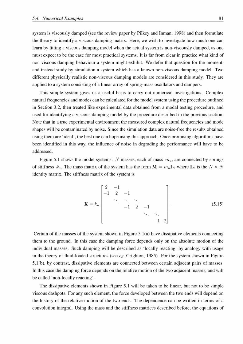
5.4. Numerical Examples 81
system is viscously damped (see the review paper by Pilkey and Inman, 1998) and then formulatethe theory to identify a viscous damping matrix. Here, we wish to investigate how much one canlearn by fitting a viscous damping model when the actual system is non-viscously damped, as onemust expect to be the case for most practical systems. It is far from clear in practice what kind ofnon-viscous damping behaviour a system might exhibit. We defer that question for the moment,and instead study by simulation a system which has a known non-viscous damping model. Twodifferent physically realistic non-viscous damping models are considered in this study. They areapplied to a system consisting of a linear array of spring-mass oscillators and dampers.
This simple system gives us a useful basis to carry out numerical investigations. Complexnatural frequencies and modes can be calculated for the model system using the procedure outlinedin Section 3.2, then treated like experimental data obtained from a modal testing procedure, andused for identifying a viscous damping model by the procedure described in the previous section.Note that in a true experimental environment the measured complex natural frequencies and modeshapes will be contaminated by noise. Since the simulation data are noise-free the results obtainedusing them are ‘ideal’, the best one can hope using this approach. Once promising algorithms havebeen identified in this way, the influence of noise in degrading the performance will have to beaddressed.
Figure 5.1 shows the model systems. N masses, each of mass mu, are connected by springsof stiffness ku. The mass matrix of the system has the form M = muIN where IN is the N × N
identity matrix. The stiffness matrix of the system is
K = ku
2 −1−1 2 −1
. . . . . . . . .−1 2 −1
. . . . . .−1 2
. (5.15)
Certain of the masses of the system shown in Figure 5.1(a) have dissipative elements connectingthem to the ground. In this case the damping force depends only on the absolute motion of theindividual masses. Such damping will be described as ‘locally reacting’ by analogy with usagein the theory of fluid-loaded structures (see eg. Crighton, 1985). For the system shown in Figure5.1(b), by contrast, dissipative elements are connected between certain adjacent pairs of masses.In this case the damping force depends on the relative motion of the two adjacent masses, and willbe called ‘non-locally reacting’.
The dissipative elements shown in Figure 5.1 will be taken to be linear, but not to be simpleviscous dashpots. For any such element, the force developed between the two ends will depend onthe history of the relative motion of the two ends. The dependence can be written in terms of aconvolution integral. Using the mass and the stiffness matrices described before, the equations of

82 Chapter 5. Identification of Viscous Damping
(a)
(b)
m
. . .
. . .
uk uk umuk um uk um uk
umukum
ukumukuk
g(t)
g(t)
g(t)
N- th
N- th
um uk
u
Figure 5.1: Linear array of N spring-mass oscillators, N = 30, mu = 1 Kg, ku = 4× 10³N/m
motion can thus be expressed in the form
Mq(t) + C
∫ t
−∞g(t− τ) q(τ) dτ + Kq(t) = 0 (5.16)
where g(t) is the damping function (assumed to have the same form for all the damping elementsin the system) and C is the associated coefficient matrix which depends on the distribution of thedampers. Two specific damping models will be considered, defined by two different forms of g(t):
MODEL 1: g(1)(t) = µ1e−µ1t; t ≥ 0 (5.17)
MODEL 2: g(2)(t) = 2
õ2
πe−µ2t2 ; t ≥ 0 (5.18)
where µ1 and µ2 are constants. Any physically realistic damping model must satisfy a conditionof positive energy dissipation at all frequencies. A sufficient condition to guarantee this, satisfiedby both models considered here, will be described in Chapter 6.
It is convenient to normalize the functions to make comparisons between models meaningful.Both functions have already been scaled so as to have unit area when integrated to infinity. Thismakes them directly comparable with the viscous model, in which the corresponding dampingfunction would be a unit delta function, g(t) = δ(t), and the coefficient matrix C would be theusual damping matrix. It is also convenient to define a characteristic time constant θj for eachdamping function, via the first moment of g(j)(t):
θj =
∫ ∞
0
t g(j)(t) dt (5.19)
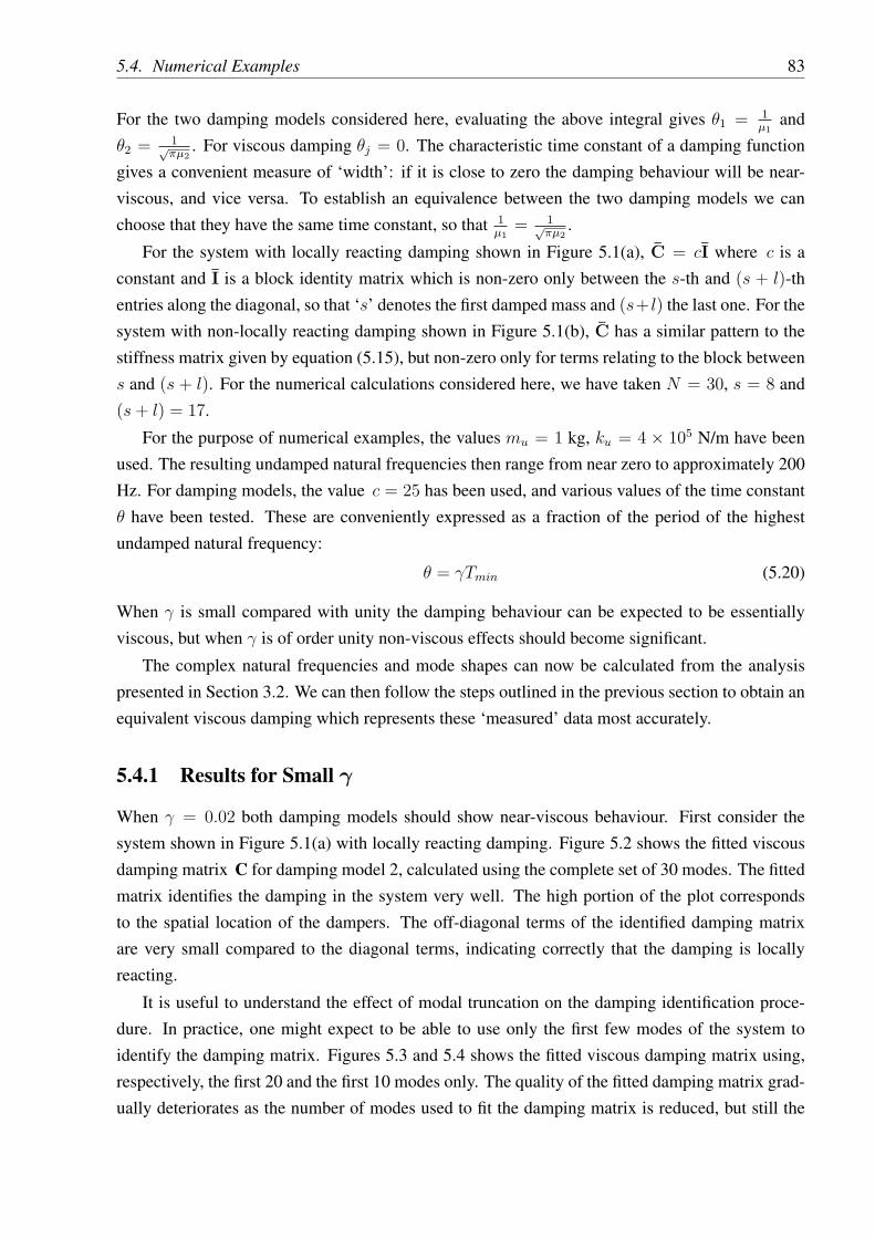
5.4. Numerical Examples 83
For the two damping models considered here, evaluating the above integral gives θ1 = 1µ1
andθ2 = 1√
πµ2. For viscous damping θj = 0. The characteristic time constant of a damping function
gives a convenient measure of ‘width’: if it is close to zero the damping behaviour will be near-viscous, and vice versa. To establish an equivalence between the two damping models we canchoose that they have the same time constant, so that 1
µ1= 1√
πµ2.
For the system with locally reacting damping shown in Figure 5.1(a), C = cI where c is aconstant and I is a block identity matrix which is non-zero only between the s-th and (s + l)-thentries along the diagonal, so that ‘s’ denotes the first damped mass and (s+ l) the last one. For thesystem with non-locally reacting damping shown in Figure 5.1(b), C has a similar pattern to thestiffness matrix given by equation (5.15), but non-zero only for terms relating to the block betweens and (s + l). For the numerical calculations considered here, we have taken N = 30, s = 8 and(s + l) = 17.
For the purpose of numerical examples, the values mu = 1 kg, ku = 4 × 10⁵ N/m have beenused. The resulting undamped natural frequencies then range from near zero to approximately 200Hz. For damping models, the value c = 25 has been used, and various values of the time constantθ have been tested. These are conveniently expressed as a fraction of the period of the highestundamped natural frequency:
θ = γTmin (5.20)
When γ is small compared with unity the damping behaviour can be expected to be essentiallyviscous, but when γ is of order unity non-viscous effects should become significant.
The complex natural frequencies and mode shapes can now be calculated from the analysispresented in Section 3.2. We can then follow the steps outlined in the previous section to obtain anequivalent viscous damping which represents these ‘measured’ data most accurately.
5.4.1 Results for Small γ
When γ = 0.02 both damping models should show near-viscous behaviour. First consider thesystem shown in Figure 5.1(a) with locally reacting damping. Figure 5.2 shows the fitted viscousdamping matrix C for damping model 2, calculated using the complete set of 30 modes. The fittedmatrix identifies the damping in the system very well. The high portion of the plot correspondsto the spatial location of the dampers. The off-diagonal terms of the identified damping matrixare very small compared to the diagonal terms, indicating correctly that the damping is locallyreacting.
It is useful to understand the effect of modal truncation on the damping identification proce-dure. In practice, one might expect to be able to use only the first few modes of the system toidentify the damping matrix. Figures 5.3 and 5.4 shows the fitted viscous damping matrix using,respectively, the first 20 and the first 10 modes only. The quality of the fitted damping matrix grad-ually deteriorates as the number of modes used to fit the damping matrix is reduced, but still the
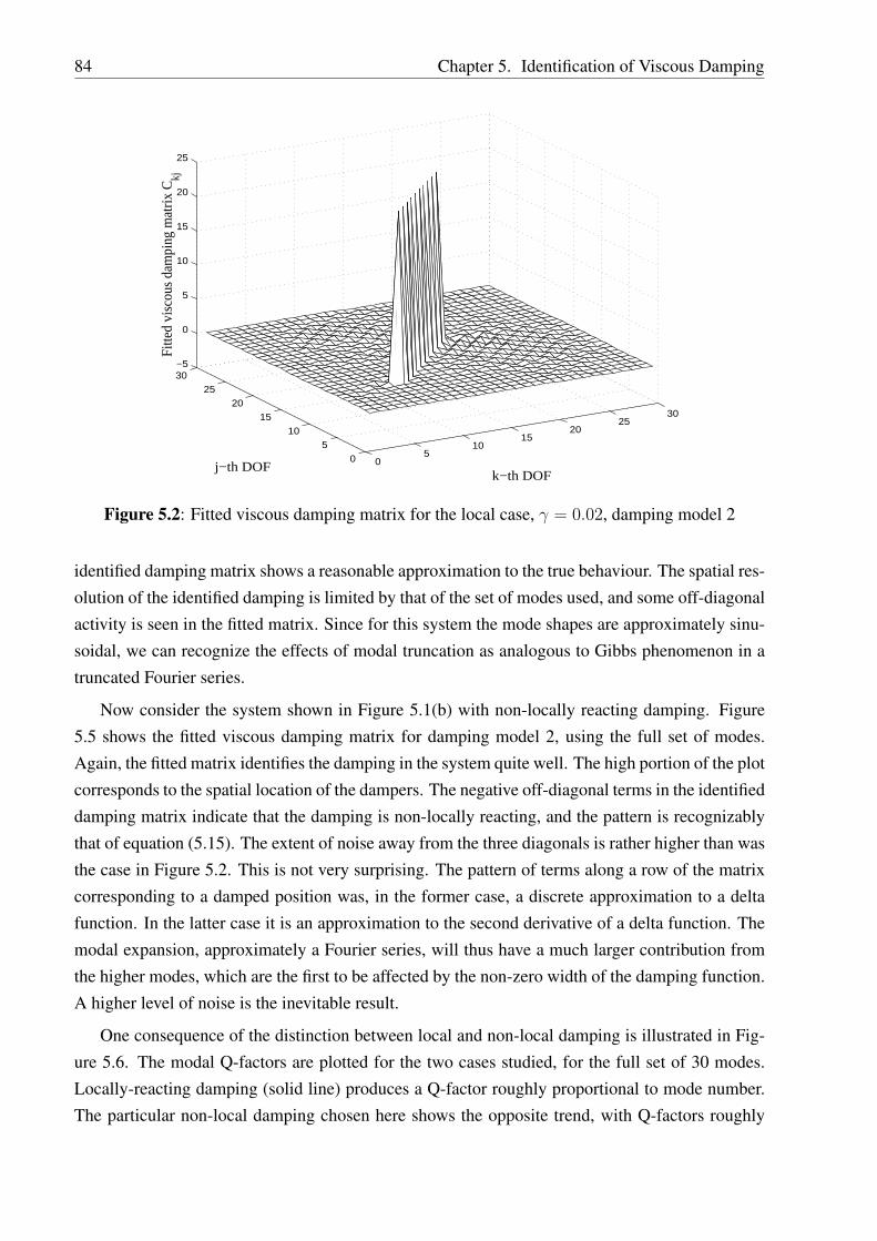
84 Chapter 5. Identification of Viscous Damping
05
1015
2025
30
0
510
15
2025
30−5
0
5
10
15
20
25
k−th DOFj−th DOF
Fitt
ed v
isco
us d
ampi
ng m
atrix
C kj
Figure 5.2: Fitted viscous damping matrix for the local case, γ = 0.02, damping model 2
identified damping matrix shows a reasonable approximation to the true behaviour. The spatial res-olution of the identified damping is limited by that of the set of modes used, and some off-diagonalactivity is seen in the fitted matrix. Since for this system the mode shapes are approximately sinu-soidal, we can recognize the effects of modal truncation as analogous to Gibbs phenomenon in atruncated Fourier series.
Now consider the system shown in Figure 5.1(b) with non-locally reacting damping. Figure5.5 shows the fitted viscous damping matrix for damping model 2, using the full set of modes.Again, the fitted matrix identifies the damping in the system quite well. The high portion of the plotcorresponds to the spatial location of the dampers. The negative off-diagonal terms in the identifieddamping matrix indicate that the damping is non-locally reacting, and the pattern is recognizablythat of equation (5.15). The extent of noise away from the three diagonals is rather higher than wasthe case in Figure 5.2. This is not very surprising. The pattern of terms along a row of the matrixcorresponding to a damped position was, in the former case, a discrete approximation to a deltafunction. In the latter case it is an approximation to the second derivative of a delta function. Themodal expansion, approximately a Fourier series, will thus have a much larger contribution fromthe higher modes, which are the first to be affected by the non-zero width of the damping function.A higher level of noise is the inevitable result.
One consequence of the distinction between local and non-local damping is illustrated in Fig-ure 5.6. The modal Q-factors are plotted for the two cases studied, for the full set of 30 modes.Locally-reacting damping (solid line) produces a Q-factor roughly proportional to mode number.The particular non-local damping chosen here shows the opposite trend, with Q-factors roughly

5.4. Numerical Examples 85
05
1015
2025
30
0
510
15
2025
30−5
0
5
10
15
20
k−th DOFj−th DOF
Fitt
ed v
isco
us d
ampi
ng m
atrix
C kj
Figure 5.3: Fitted viscous damping matrix using first 20 modes for the local case, γ = 0.02,damping model 2
05
1015
2025
30
0
510
15
2025
30−2
0
2
4
6
8
10
k−th DOFj−th DOF
Fitt
ed v
isco
us d
ampi
ng m
atrix
C kj
Figure 5.4: Fitted viscous damping matrix using first 10 modes for the local case, γ = 0.02,damping model 2
inversely proportional to mode number (dashed line). Both trends can be understood in terms ofRayleigh damping. If the damping extended over the entire structure rather that being limited to afinite patch, then the local-reacting damping would correspond to a dissipation matrix proportionalto the mass matrix, while the non-local damping would correspond to a dissipation matrix propor-

86 Chapter 5. Identification of Viscous Damping
05
1015
2025
30
0
510
15
2025
30−30
−20
−10
0
10
20
30
40
50
k−th DOFj−th DOF
Fitt
ed v
isco
us d
ampi
ng m
atrix
C kj
Figure 5.5: Fitted viscous damping matrix for the non-local case, γ = 0.02, damping model 2
tional to the stiffness matrix. The trends of modal Q-factor with frequency would then be exactlyproportional and inversely proportional, respectively. Limiting the damping to a part of the struc-ture has evidently not disturbed this pattern very much. The variation with frequency has translatedinto a variation with mode number: the mode number relates rather directly to wavenumber for thissimple system, and the physical origins of the different trends of Q-factors lies in dependence onwavelength, rather than on frequency as such.
When the fitting procedure is repeated using the alternative damping model of equation (5.17)the results are sufficiently similar that they are not reproduced here. Since the time constant isso short, both damping models are near to viscous damping and the detailed difference in theirfunctional behaviour does not influence the results significantly. In summary, we can say thatwhen the time constant for a damping model is small the proposed identification method worksquite well regardless of the functional form of the damping mechanism. The spatial location ofdamping is revealed clearly, and whether it is locally or non-locally reacting. Modal truncationblurs the results, but does not invalidate the identification process.
5.4.2 Results for Larger γ
When γ is larger the two non-viscous damping models depart from the viscous damping model,each in its own way. For the value γ = 0.5, Figure 5.7 shows the result of running the fittingprocedure for damping model 1 (equation (5.17)) with locally-reacting damping and the full set ofmodes, similar to Figure 5.2. Figure 5.8 shows the corresponding fitted viscous damping matrixC for damping model 2 (equation (5.18)). In both cases it may be noted that although we have
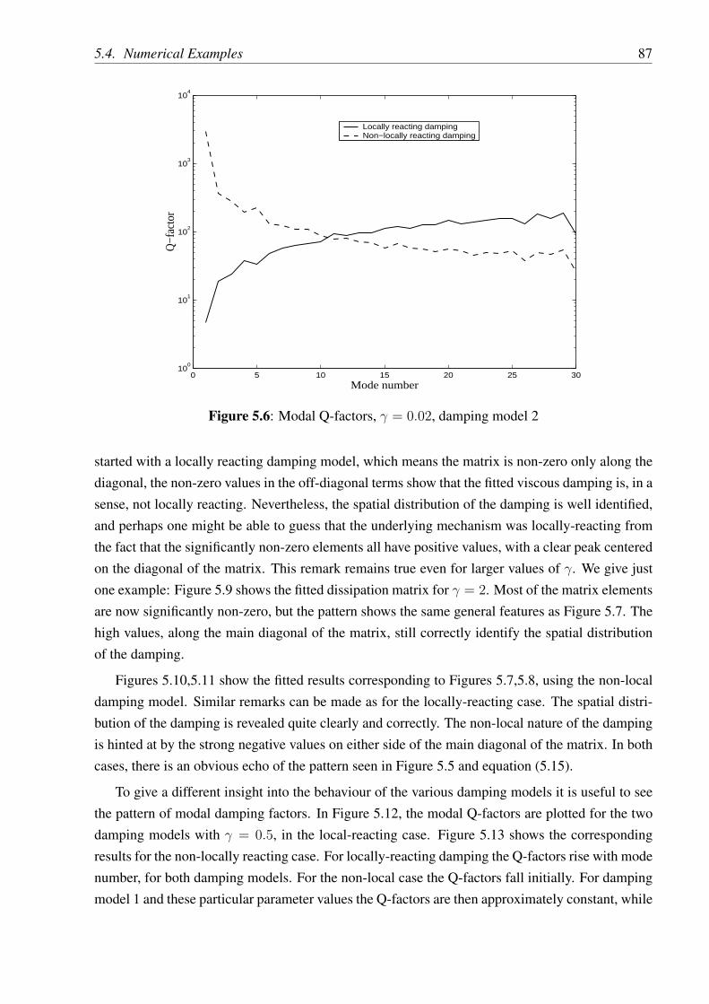
5.4. Numerical Examples 87
0 5 10 15 20 25 3010
0
101
102
103
104
Mode number
Q−f
acto
r
Locally reacting damping Non−locally reacting damping
Figure 5.6: Modal Q-factors, γ = 0.02, damping model 2
started with a locally reacting damping model, which means the matrix is non-zero only along thediagonal, the non-zero values in the off-diagonal terms show that the fitted viscous damping is, in asense, not locally reacting. Nevertheless, the spatial distribution of the damping is well identified,and perhaps one might be able to guess that the underlying mechanism was locally-reacting fromthe fact that the significantly non-zero elements all have positive values, with a clear peak centeredon the diagonal of the matrix. This remark remains true even for larger values of γ. We give justone example: Figure 5.9 shows the fitted dissipation matrix for γ = 2. Most of the matrix elementsare now significantly non-zero, but the pattern shows the same general features as Figure 5.7. Thehigh values, along the main diagonal of the matrix, still correctly identify the spatial distributionof the damping.
Figures 5.10,5.11 show the fitted results corresponding to Figures 5.7,5.8, using the non-localdamping model. Similar remarks can be made as for the locally-reacting case. The spatial distri-bution of the damping is revealed quite clearly and correctly. The non-local nature of the dampingis hinted at by the strong negative values on either side of the main diagonal of the matrix. In bothcases, there is an obvious echo of the pattern seen in Figure 5.5 and equation (5.15).
To give a different insight into the behaviour of the various damping models it is useful to seethe pattern of modal damping factors. In Figure 5.12, the modal Q-factors are plotted for the twodamping models with γ = 0.5, in the local-reacting case. Figure 5.13 shows the correspondingresults for the non-locally reacting case. For locally-reacting damping the Q-factors rise with modenumber, for both damping models. For the non-local case the Q-factors fall initially. For dampingmodel 1 and these particular parameter values the Q-factors are then approximately constant, while

88 Chapter 5. Identification of Viscous Damping
05
1015
2025
30
0
510
15
2025
30−1
0
1
2
3
4
5
6
7
8
k−th DOFj−th DOF
Fitt
ed v
isco
us d
ampi
ng m
atrix
C kj
Figure 5.7: Fitted viscous damping matrix for the local case, γ = 0.5, damping model 1
05
1015
2025
30
0
510
15
2025
30−1
0
1
2
3
4
5
6
k−th DOFj−th DOF
Fitt
ed v
isco
us d
ampi
ng m
atrix
C kj
Figure 5.8: Fitted viscous damping matrix for the local case, γ = 0.5, damping model 2
for damping mode 2 they rise again after a while, reaching very high values at high mode numbers.In terms of physical plausibility, damping model 1 in the non-local configuration gives the closestmatch to the common practical experience that modal damping factors are approximately constant.However, physical plausibility is not a major issue here, where the aim is to test the procedureunder a wide range of circumstances.

5.4. Numerical Examples 89
05
1015
2025
30
0
510
15
2025
30−0.5
0
0.5
1
1.5
2
k−th DOFj−th DOF
Fitt
ed v
isco
us d
ampi
ng m
atrix
C kj
Figure 5.9: Fitted viscous damping matrix for the local case, γ = 2.0, damping model 1
0
5
10
15
20
25
30
05
1015
2025
30−4
−2
0
2
4
6
8
k−th DOFj−th DOF
Fitt
ed v
isco
us d
ampi
ng m
atrix
C kj
Figure 5.10: Fitted viscous damping matrix for the non-local case, γ = 0.5, damping model 1
To judge the numerical accuracy of the fitted viscous damping it is useful to reconstruct transferfunctions. It is easy to do this, by inverting the dynamic stiffness matrix using the fitted viscousdamping matrix. A typical transfer function Hkj(ω), for k = 11 and j = 24 is shown in Figure5.14, based on locally-reacting damping using damping model 1. It is clear that the reconstructedtransfer function agrees well with the original one. This is to be expected: the fitting procedure

90 Chapter 5. Identification of Viscous Damping
0
5
10
15
20
25
30
05
1015
2025
30−2
−1
0
1
2
k−th DOFj−th DOF
Fitt
ed v
isco
us d
ampi
ng m
atrix
C kj
Figure 5.11: Fitted viscous damping matrix for the non-local case, γ = 0.5, damping model 2
outlined in the previous section is exact, within the the approximations of the small-damping per-turbation theory, provided the full set of modes is used. The full set of poles and their residues arecorrectly reproduced — this is the essential contrast between this approach and one which fits onlyproportional damping, for which the poles can be correct but the residues cannot (because they willbe real, not complex). This result has a far-reaching implication: an incorrect damping model (thefitted viscous damping) with a different spatial distribution from the true locally-reacting modelcan reproduce accurately the full set of transfer functions. This means that by measuring transferfunctions it is not possible to identify uniquely the governing mechanism.
However, it should be noted that in all cases of Figures 5.7−5.11 the fitted damping matrix isnot symmetric. This is, in some sense, a non-physical result. In view of this non-symmetry, it isinteresting to check the reciprocity of the transfer functions. In Figure 5.14 the reciprocal transferfunction Hjk(ω) is also plotted, as a dashed line. It is not visible as a separate line in the figure,because it matches Hkj(ω) to good accuracy. This plot demonstrates that the non-symmetry ofthe fitted viscous damping in the spatial coordinate does not necessarily affect the reciprocity ofthe transfer functions. Instead, we should regard non-symmetry of a fitted dissipation matrix asevidence that the true damping model is not viscous. To obtain a correct physical description ofthe damping, a non-viscous model should be fitted instead. This idea is developed in Chapter 6.

5.4. Numerical Examples 91
0 5 10 15 20 25 3010
0
101
102
103
104
105
106
Mode number
Q−fa
ctor
Model 1Model 2
Figure 5.12: Modal Q-factors for the local case, γ = 0.5
0 5 10 15 20 25 3010
2
103
104
105
106
Mode number
Q−f
acto
r
Model 1Model 2
Figure 5.13: Modal Q-factors for the non-local case, γ = 0.5

92 Chapter 5. Identification of Viscous Damping
0 200 400 600 800 1000 1200−170
−160
−150
−140
−130
−120
−110
−100
−90
−80
Frequency (rad/s)
Tran
sfer F
uncti
on (d
B)
Exact Hk,j
Fitted H
k,jFitted H
j,k
Figure 5.14: Transfer functions for the local case, γ = 0.5, damping model 1, k = 11, j = 24
5.5 Conclusions
In this chapter a method has been proposed to identify a non-proportional viscous damping matrixin vibrating systems. It is assumed that damping is light so that the first order perturbation methodis applicable. The method is simple, direct, and compatible with conventional modal testing proce-dures. The complex modes and natural frequencies are used, but the method does not require eitherthe full set of modal data, or any knowledge of the mass and stiffness matrices. The validity of theproposed method has been explored by applying it to simulated data from a simple test problem,in which a linear array of spring-mass oscillators is damped by non-viscous elements over part ofits length.
Numerical experiments have been carried out with a wide range of parameter values and dif-ferent damping models. The main features of the results have been illustrated by two particulardamping models and representative parameter values. It has been shown that the method generallypredicts the spatial location of the damping with good accuracy, and also gives a good indication ofwhether the damping is locally-reacting or not. Whatever the nature of the fitted damping matrix C,the transfer functions obtained from the fitted viscous damping agree well with the exact transferfunctions of the simulated system. Reciprocity of the transfer functions remains preserved withinan acceptable accuracy although in some cases the fitted viscous damping C is not symmetric.
Symmetry breaking of the fitted viscous damping matrix C depends on the value of the char-acteristic time constants θ of the damping model, defined by equation (5.19). When θ is shortcompared with the natural periods of the vibration, the damping is effectively viscous and the fit-ting procedure gives a physically-sensible symmetric matrix. When θ is larger, though, the memoryof the damping function influences the detailed behaviour. Although the poles and residues of the

5.5. Conclusions 93
transfer functions can still be fitted accurately with a model of viscous form, the underlying non-viscous behaviour manifests itself in a non-symmetrical matrix. If a correct physical description ofthe damping mechanism is needed, then a suitable non-viscous model must be selected and fitted.We take up this question in Chapter 6.

94 Chapter 5. Identification of Viscous Damping

Chapter 6
Identification of Non-viscous Damping
6.1 Introduction
Linear systems must generally be expected to exhibit non-viscous damping. In the last chapterit was shown that when a system is non-viscously damped, it is possible to fit a viscous damp-ing model to the set of measured transfer functions but that the fitted damping matrix will benon-symmetrical. The fitted model may also be misleading in other ways: for example it maypredict the wrong spatial distribution of damping over the structure. Of course, a priori selectionof viscous damping in the identification procedure rules out any possibility of recognizing otherdamping behaviour present in the structure. In this chapter we consider the identification of certainnon-viscous damping models in the context of general multiple degrees-of-freedom linear systems.
A key issue in identifying non-viscous damping is to decide on an appropriate damping modelto consider. A brief review on available damping models may be found in Section 1.2. There havebeen detailed studies of material damping and of specific structural components. Lazan (1968),Bert (1973) and Ungar (1973) have given excellent accounts of different mathematical methodsfor modelling damping in (solid) material and their engineering applications. The book by Nashifet al. (1985) presents more recent studies in this area. Other than material damping a major sourceof energy dissipation in a vibrating structure is the structural joints. Here, energy loss can takeplace through air-pumping and local frictional effects. The air-pumping phenomenon is associatedwith air trapped in pockets in the vicinity of a vibrating surface. In these situations, the air issqueezed in and out through any available gap, leading to viscous dissipation of energy. Dampingbehaviour associated with joints has been studied by many authors. For example Earls (1966) hasobtained the energy dissipation in a lap joint over a cycle under different clamping pressure. Beardsand Williams (1977) have noted that significant damping can be obtained by suitably choosing thefastening pressure to allow some interfacial slip in joints. In many cases these damping mecha-nisms turn out be locally non-linear, requiring an equivalent linearization technique for a globalanalysis (Bandstra, 1983). These studies provide useful physical insights into damping mecha-nisms, but due to their very specific nature it is not possible to formulate a general procedure foridentification of such mechanisms by simple vibration measurement.
95

96 Chapter 6. Identification of Non-viscous Damping
In Section 1.6 it was pointed out that methodologies of identification of non-viscous dampingin the context of general MDOF systems is not well developed. Banks and Inman (1991) haveproposed a somewhat general approach for identification of non-viscous damping models in Euler-Bernoulli beams. They have considered four different models of damping: viscous air damping,Kelvin-Voigt damping, time hysteresis damping and spatial hysteresis damping, and used a splineinverse procedure to form a least-square fit to the experimental data. It was observed that the spatialhysteresis model combined with a viscous air damping model gave the best quantitative agreementwith the experimental time histories. A procedure for obtaining hysteretic damping parameters infree-hanging pipe systems is given by Fang and Lyons (1994). Assuming material damping to bethe only source of damping they have given a theoretical expression for the loss factor of the n-thmode. The system-specific nature of these methods means that they cannot be extended in a simpleway to more general multiple degrees-of-freedom systems.
In Section 1.2.3 it was mentioned that convolution integral models are most general class oflinear non-viscous damping models in the context of multiple degrees-of-freedom systems. InChapter 3 it was shown that such damping models can be handled in a very similar way to viscousmodels. These results motivate us to develop procedures for identification this type of generaldamping models from standard vibration testing data. A wide variety of mathematical expressions,as shown in Table 1.1, could be used for the kernel functions. Of these, the exponential functionseems a particularly promising candidate. Cremer and Heckl (1973) have written ‘Of the manyafter-effect functions that are possible in principle, only one — the so-called relaxation function— is physically meaningful.’ They go on to give a physical justification for this model, by whichthey mean the exponential case. The argument applies most convincingly to the case of materialdamping, rather than joint damping. An alternative mathematical rationalization can be givenin terms of exponential contributions from the poles of frequency-response functions when theFourier transform is inverted (see Muravyov, 1997). With this motivation, we concentrate here onfitting exponential damping models to vibration data.
The analysis in this chapter is restricted to linear system behaviour and it is assumed that thedamping is light. In Section 6.2 we outline the expressions of complex frequencies and modesbased on the first-order perturbation method when the system is non-viscously damped. Usingthese perturbation results, a method for identification of non-viscous damping models using com-plex modes and natural frequencies is proposed. We assume that the mass matrix of the structureis known — either directly from a finite element model or by means of modal updating based onexperimental measurements. Having the mass matrix we try to identify an exponential dampingmodel consistent with the measured complex modes. In Section 6.3 a procedure to obtain the re-
laxation parameter of an exponential damping model is outlined. Identification of the associateddamping coefficient matrix is discussed in Section 6.5. The proposed method is illustrated usingsimulated numerical examples directly comparable to those in the last chapter. Finally Section 6.6summarizes the main findings of this chapter.

6.2. Background of Complex Modes 97
6.2 Background of Complex Modes
Dynamics of non-viscously damped systems has been discussed in details in Chapter 3. As men-tioned earlier, only elastic modes will be considered because non-viscous modes are not measur-able within the scope of traditional modal analysis. Thus, in the context of non-viscously dampedsystems ‘complex modes’ implies complex elastic modes. Expressions of complex modes can beobtained from the analysis presented in Section 3.2.1. One special case of this general analysis inconsidered in Section 3.2.3 when the damping is lightly non-proportional. In this section we con-sider a further special case when the damping is light so that the first-order perturbation methodcan be applied. First-order perturbation results can be obtained from the results in Section 3.2.3 asfollows.
Suppose λj, zj is j-th complex natural frequency and and complex mode shape. In the contextof the notations used in Section 3.2.3, sj = iλj . Using this, from equation (3.33) approximateexpression for the complex natural frequencies can be obtained as
λj ≈ ±ωj + iG′jj(±ωj)/2 (6.1)
where G′kl(ωj) = xT
k G(ωj)xl is the frequency dependent damping matrix expressed in normalcoordinates and G(ω) is the Fourier transform of the matrix of kernel functions G(t). Since theinverse Fourier transform of G(ω) must be real it must satisfy the condition G(−ω) = G(ω)∗,where (•)∗ denotes complex conjugation. It follows that the eigenvalues of the generally dampedsystem appear in pairs λ and −λ∗ (unless λ is purely imaginary). The first-order approximateexpression for the complex eigenvectors can be obtained as a special case of equation (3.35). Theresult is
zj ≈ xj + iN∑
k=1k 6=j
ωjG′kj(ωj)
(ω2j − ω2
k)xk. (6.2)
Equations (6.1) and (6.2) were first obtained by Woodhouse (1998). Note that the eigenvectorsalso appear in complex conjugate pairs. Since in general G′
kj(ωj) will be complex, in contrast tothe viscously damped case the real part of complex natural frequencies and complex mode shapesdo not coincide with the undamped ones. This fact will complicate the problem of fitting modelparameters to experimental complex modes.
It is natural to consider first the idealized problem in which just one relaxation function is usedfor identification purposes. In that case the general form of the kernel function in equation (3.1)reduces to
G(t) = C g(t) (6.3)
where g(t) is some damping function and C is a positive-definite coefficient matrix. The admissibleform of g(t) is restricted by the condition of non-negative energy loss given in equation (1.33). Thedamping model in equation (6.3) is physically realistic if the real part of the Fourier transform ofthe kernel function is non-negative within the driving frequency range, that is <[G(ω)] ≥ 0,∀ω.

98 Chapter 6. Identification of Non-viscous Damping
This can be easily shown. Rewriting equation (1.33) in the frequency domain and using (6.3), therate of energy dissipation can be expressed as
F (ω) =ω2
2<
q∗T C qG(ω)
(6.4)
where <(•) represents the real part of (•) and F (ω), q and G(ω) are the Fourier transform of F(t),q(t) and g(t) respectively. For a physically realistic model of damping we must have
F (ω) ≥ 0
orω2
2<
q∗T C qG(ω)
≥ 0
or <G(ω) ≥ 0
(6.5)
since for a real value of driving frequency ω2 ≥ 0 and q can be chosen in a way that<
q∗T C q≥
0 as C is positive definite.
6.3 Fitting of the Relaxation Parameter
As has been mentioned earlier, from the wide range of non-viscous damping models the exponen-tial function seems a particularly good candidate. It satisfies the condition (6.5) at all frequencies.In this section we outline a general method to fit the relaxation parameter of an exponential damp-ing model using measured modal data.
6.3.1 Theory
We assume that the damping has only one relaxation function, so that the matrix of kernel functionsis of the form
G(t) = µe−µt C (6.6)
where µ is the relaxation parameter and C is the associated coefficient matrix. The factor µ servesto normalize the kernel function: see Section 6.3.2. Complex natural frequencies and mode shapesfor systems with this kind of damping can be obtained from equations (6.1) and (6.2). In view ofthe expression for damping given in equation (6.6) it is easy to see that the term G′
kj(ωj) appearingin these equations can be expressed as
G′kj(ωj) =
µ
µ + iωj
C ′kj =
[µ2
µ2 + ω2j
− iµωj
µ2 + ω2j
]C ′
kj (6.7)
where C ′kj = xT
k Cxj . Using this expression in equation (6.1), the j-th complex natural frequencyis given by
λj ≈ ωj + iC ′
jj
2
[µ2
µ2 + ω2j
− iµωj
µ2 + ω2j
]. (6.8)

6.3. Fitting of the Relaxation Parameter 99
Similarly from equation (6.2) the j-th complex mode can be expressed as
zj ≈ xj +N∑
k=1k 6=j
µωj
(µ2 + ω2j )
ωjC′kj
(ω2j − ω2
k)xk + i
N∑k=1k 6=j
µ2
(µ2 + ω2j )
ωjC′kj
(ω2j − ω2
k)xk. (6.9)
Suppose that λj and zj for j = 1, 2, · · ·m are the measured complex natural frequencies andmodes. Write
zj = uj + ivj. (6.10)
Here zj ∈ CN where N denotes the number of measurement points on the structure and thenumber of modes considered in the study is m. In general m 6= N , usually N ≥ m. Assumethat xj ∈ RN are the undamped modes and µ is the relaxation parameter to be estimated from theexperiment. In order to fit a damping model of the form (6.6), equations (6.8) and (6.9) must bevalid in conjunction with the experimental measurements λj and zj . As an initial approximationwe may suppose the real part of the complex natural frequencies to be the same as the undampednatural frequencies:
ω(0)j = <
(λj
). (6.11)
For most practical cases it turns out that the above value of ω(0)j is sufficiently accurate to carry out
further analysis. However, we present later an iterative method which may be used to update thevalue of ωj and remove the need for this approximation (see Section 6.5.2 for details).
In view of equations (6.9) and (6.10) and considering that only m modes are measured, sepa-rating real and imaginary parts of uj gives
uj = <(zj) ≈ xj +m∑
k=1k 6=j
Akjxk; where Akj =µωj
(µ2 + ω2j )
Bkj (6.12)
and
vj = =(zj) ≈m∑
k=1k 6=j
Bkjxk; where Bkj =µ2
(µ2 + ω2j )
Bkj. (6.13)
Here the unknown constants Bkj are defined as
Bkj =ωjC
′kj
ω2j − ω2
k
. (6.14)
It may be noted that in addition to Bkj , the relaxation constant µ and the undamped modes xk arealso unknown. Combining equations (6.12) and (6.13) one can write
uj = xj +ωj
µvj. (6.15)
From the preceding equation it is clear that if µ À ωj , then uj → xj . This implies that whenthe damping mechanism is near to viscous, the real part of each complex mode tends towards

100 Chapter 6. Identification of Non-viscous Damping
the corresponding undamped mode. Since the undamped modes are orthonormal with respect tothe mass matrix, from equation (6.13) it may be observed that the imaginary part of each complexmode vj is M-orthogonal to its corresponding undamped mode so that vT
j Mxj = 0. Premultiplyingequation (6.15) by vT
j M one can write
vTj Muj = vT
j Mxj +ωj
µvT
j Mvj (6.16)
Now use of the orthogonality property of vj and xj leads to
µj =ωjv
Tj Mvj
vTj Muj
. (6.17)
We have used the notation µj because for different choices of j on the right hand side one willin general obtain different values of µ. If in practice one obtained very similar values, this wouldconfirm the initial assumption that the actual system has only one relaxation time. On the otherhand, if significantly different values are obtained it would indicate that the assumed model needsto be extended. We show shortly that the pattern of variation of µj can give some clues about thetrue underlying model. If one wished to choose a single value of µ to best represent a range ofvalues found by this procedure, one could consider several alternatives:
1. Simply select a value of j, say j = k ≤ m, to obtain µ. For this choice
µ =ωkv
Tk Mvk
vTk Muk
. (6.18)
How to select the value of k will be discussed in the next subsection.
2. Average the realizations of µ. For this choice
µ =1
mµ
mµ∑j=1
ωjvTj Mvj
vTj Muj
. (6.19)
where mµ ≤ m are the number of terms to be retained.
3. Sum the numerator and denominator separately and take their ratio to obtain µ. For thischoice
µ =
∑mµ
j=1 ωjvTj Mvj∑mµ
j=1 vTj Muj
. (6.20)
We can best illustrate via a numerical example.
6.3.2 Simulation Method
Numerical studies have been carried out using simulated systems identical to those used in Chapter5. Figure 6.1 shows the model systems together with the numerical values used. For these param-eter values the resulting undamped natural frequencies range from near zero to approximately 200

6.3. Fitting of the Relaxation Parameter 101
Hz. The damping elements are associated with masses between the s-th and (s + l)-th (N = 30,s = 8 and (s + l) = 17 are taken for the numerical calculations). For the system shown in Fig-ure 6.1(a) the damping force depends only on the absolute motion of the individual masses. Suchdamping will be described as ‘locally reacting’. For the system shown in Figure 6.1(b), by con-trast, dissipative elements are connected between certain adjacent pairs of masses. In this casethe damping force depends on the relative motion of the two adjacent masses, and will be called‘non-locally reacting’. In the previous chapter, a viscous damping matrix was calculated from thecomplex modes and frequencies of these systems. Here we seek to identify the parameters of anexponential damping model using the same modal data.
(a)
(b)
m
. . .
. . .
uk uk umuk um uk um uk
umukum
ukumukuk
g(t)
g(t)
g(t)
N- th
N- th
um uk
u
Figure 6.1: Linear array of N spring-mass oscillators, N = 30, mu = 1 Kg, ku = 4× 10³N/m.
The dissipative elements shown in Figure 6.1 are taken to be linear non-viscous dampers sothat the equations of motion are described by (5.16). Three damping models, two of which wereconsidered in 5, are used: one with an exponential kernel function as assumed in the model beingfitted, and two others with different functions to probe the limitations of the fitting procedure. Theyare determined by three different forms of g(t) (defined in equation (6.3)):
• MODEL 1 (exponential):
g(1)(t) = µ1e−µ1t (6.21)
• MODEL 2 (Gaussian):
g(2)(t) = 2
õ2
πe−µ2t2 (6.22)

102 Chapter 6. Identification of Non-viscous Damping
• MODEL 3 (double exponential or GHM):
g(3)(t) =β1µ3e
−µ3t + β2µ4e−µ4t
β1 + β2
(6.23)
All the three damping models are normalized such that the damping functions have unit area whenintegrated to infinity, i.e., ∫ ∞
0
g(j)(t) dt = 1. (6.24)
This will make them directly comparable with the viscous model, in which the correspondingdamping function would be a unit delta function, g(t) = δ(t), and the coefficient matrix C wouldbe the usual dissipation matrix. For each damping function a characteristic time constant can bedefined via the first moment of g(j)(t):
θ(j) =
∫ ∞
0
t g(j)(t) dt. (6.25)
For the three damping models considered here, evaluating this integral gives
θ(1) =1
µ1
(6.26)
θ(2) =1√πµ2
(6.27)
θ(3) =β1/µ3 + β2/µ4
β1 + β2
. (6.28)
Note that for viscous damping θ = 0. The characteristic time constant of a damping function givesa convenient measure of ‘width’: if it is close to zero the damping behaviour will be near-viscous,and vice versa. For comparability between the three damping models we take them all to have thesame time constant.
Complex natural frequencies and modes of the systems are calculated using equations (6.1)and (6.2), then these are treated as if they were experimental data obtained from a modal testingprocedure. The procedures described above can be applied to identify the relaxation parameterof an exponential damping model. We present results of the fitting procedure for both small andlarge values of the characteristic time constant, expressed in non-dimensional form as given byequation (5.20). When γ is small compared with unity the damping behaviour can be expected tobe essentially viscous, but when γ is of order unity or bigger non-viscous effects are likely to besignificant.
6.3.3 Numerical ResultsResults for Small γ
We consider first γ = 0.02, so that damping models show near-viscous behaviour. Since theviscous model is a special case of the exponential model we might expect good fit quality in this

6.3. Fitting of the Relaxation Parameter 103
case. For the system shown in Figure 6.1(a) with locally reacting damping, Figure 6.2 shows thevalues of γ obtained from µ (recall that γ = 1
Tminµ) for all j = 1, · · · , 30 for Gaussian damping
(model 2). In the same Figure the values of γ corresponding to equations (6.19) and (6.20) usingmµ = 30 are also shown. Because the damping mechanism is near to viscous the fitted values ofγ are quite small, and in fact agree well with the assumed γ = 0.02 for all values of j. To obtaina single ‘best’ value any one of the three relationships in equations (6.18) – (6.20) could be used.Similar features were observed (results not shown) when the fitting procedure was repeated for thenon-locally damped case shown in Figure 6.1(b).
0 5 10 15 20 25 300.0199
0.02
0.0201
0.0202
Mode number
Ori
gina
l and
fitte
d γ
Fitted γ for different modes Fitted using Eq. (6.19), γ
fit= 0.020033
Fitted using Eq. (6.20), γfit
= 0.020071
Original γ = 0.02
Figure 6.2: Values of γ obtained from different µ calculated using equations (6.18)–(6.20) for thelocal case, damping model 2
Now we turn our attention to the systems with double exponential damping model (model 3).It is supposed that the two exponential functions combine to give a value γ = 0.02. In this casewe consider β1 = 0.5, γ3 = 0.01 and β2 = 0.5, γ4 = 0.03. Values of γ obtained for differentmodes for the locally reacting case with this damping model is shown in Figure 6.3. In the samefigure we also show the values of γ corresponding to equation (6.19) and (6.20). Again, as in thecase of damping model 2 discussed above, the fitted values of γ are all very close to the correctvalue γ = 0.02. The only difference from the previous case is that values now decrease slightlywith j rather than increasing. Similar features were observed (results not shown) when the fittingprocedure is extended to non-locally damped systems with damping model 3. We conclude that,when the damping is near to viscous, regardless of the functional form or damping type, the fittingprocedure gives a good estimate of the damping time constant and that any one of the relationshipin equations (6.18) – (6.20) may be used to obtain the ‘best’ relaxation parameter.

104 Chapter 6. Identification of Non-viscous Damping
0 5 10 15 20 25 300.0198
0.0199
0.02
0.0201
Mode number
Ori
gina
l and
fitte
d γ
Fitted γ for different modes Fitted using Eq. (6.19), γ
fit= 0.019914
Fitted using Eq. (6.20), γfit
= 0.01984
Original γ= 0.02
Figure 6.3: Values of γ obtained from different µ calculated using equations (6.18)–(6.20) for thelocal case, damping model 3
Results for Larger γ
When γ is larger the three damping models depart more strongly from the viscous damping modeleach in its own way. Also, model 1, which is used for fitting purpose, differ form the other twodamping models. We show typical results for the case γ = 0.5. When the fitting procedure isrun for damping model 1, the calculation correctly reproduces the assumed γ value for all modesbecause the model being fitted is precisely the one assumed by the theory. This confirms theaccuracy of the computer coding, but nothing further is to be learnt from displaying the results.Figure 6.4 shows the values of γ obtained for each mode for damping model 2 applied to thelocally reacting system. The value of γ now vary considerably with j. This indicate, of course,that the assumption of a single kernel is not correct for this system. As will be discussed shortly,the variation of γ with j gives some clue as to the correct form of the kernel function. Estimatesof γ obtained from equations (6.19) and (6.20) using mµ = 30 are also shown in Figure 6.4. Boththese estimates are higher than the value of γ used for simulation and also the estimate obtainedusing equation (6.19) is higher than that obtained using equation (6.20). Observe that the valueof γ obtained using equation (6.18) with k = 1 (marked by a *) is very close to the value of theoriginal γ used in the simulation. An explanation of this behaviour is given in Section 6.4. It isshown there that under rather general circumstances, a value of γ obtained from equation (6.18)with k = 1 is likely to be a good estimate of the correct characteristic time constant defined viathe first moment as in equation (5.20). Results for the non-local case are shown in Figure 6.5. Asimilar trend is seen to that in Figure 6.4. In this figure also we observe that the value of γ obtained

6.4. Selecting the Value of µ 105
from equation (6.18) with k = 1 (marked by a *) is very close to the value of the original γ whilethose obtained from equations (6.19) and (6.20) differ significantly from the original one. Alsoobserve that estimates of γ obtained from the two former equations are higher than the simulatedvalue for both the local and nonlocal systems. However, unlike the case of Figure 6.4, here thevalue of γ obtained from equation (6.19) is lower than that obtained using equation (6.20).
0 5 10 15 20 25 3010
−1
100
101
102
Mode number
Ori
gina
l and
fitte
d γ
Fitted γ for different modes Fitted using Eq. (6.19), γ
fit= 1.5642
Fitted using Eq. (6.20), γfit
= 0.63666
Original γ = 0.5
Figure 6.4: Values of γ obtained from different µ calculated using equations (6.18)–(6.20) for thelocal case, damping model 2
Now consider damping model 3, consisting of two exponential functions. For the numericalvalues we take: β1 = 0.5, γ3 = 0.2 and β2 = 0.5, γ4 = 0.8. This results an equivalent γ for themodel of 0.5, the same as for damping model 2 discussed above. Figure 6.6 shows the values of γ
obtained for each mode for this damping model applied to the locally reacting system. This timeγ decreases with j, in contrast to the Gaussian case. The range of variation is less dramatic, butstill significant. Observe that, as with damping model 2, the value of γ obtained from equation(6.18) with k = 1 (marked by a *) is very close to the value of the original γ used in the simulationwhile that obtained from equations (6.19) and (6.20) differ significantly from the original one.However, unlike the case of damping model 2, here the estimates of γ obtained from the two formerequations are lower than the simulated value. Behaviour analogous to this was also observed whenthe identification procedure is repeated for the nonlocally damped system.
6.4 Selecting the Value of µ
From equations (6.18) – (6.20) it is clear that different choices of j yield different values of µ,which contradicts our initial assumption that the system has only one relaxation time. Here it

106 Chapter 6. Identification of Non-viscous Damping
0 5 10 15 20 25 3010
−1
100
101
102
Mode number
Ori
gina
l and
fitte
d γ
Fitted γ for different modes Fitted using Eq. (6.19), γ
fit= 1.5722
Fitted using Eq. (6.20), γfit
= 2.813
Original γ = 0.5
Figure 6.5: Values of γ obtained from different µ calculated using equations (6.18)–(6.20) for thenon-local case, damping model 2
0 5 10 15 20 25 300.1
0.2
0.3
0.4
0.5
0.6
0.7
0.8
0.9
Mode number
Orig
inal
and
fitte
d γ
Fitted γ for different modes Fitted using Eq. (6.19), γ
fit= 0.29049
Fitted using Eq. (6.20), γfit
= 0.25898
Original γ= 0.5 γ for 2 functions
Figure 6.6: Values of γ obtained from different µ calculated using equations (6.18)–(6.20) for thelocal case, damping model 3
will be shown that for systems with normalized damping functions similar to equations (6.21) and(6.22) the best estimate of µ is given by equation (6.18) with k = 1.
Since the damping functions are normalized to have unit area when integrated to infinity they

6.4. Selecting the Value of µ 107
can be written in the form
g(t) = β f(t); where β =1∫∞
0f(t)dt
. (6.29)
The characteristic time constant is obtained from equation (6.25) as
θ =
∫∞0
t f(t)dt∫∞0
f(t)dt. (6.30)
It is useful to express this result in the frequency domain. From the definition of the Fouriertransform
F (ω) =
∫ ∞
0
f(t)e−iωtdt, (6.31)
differentiating with respect to ω we have
F ′(ω) =dF (ω)
dω=
∫ ∞
0
−itf(t)e−iωtdt. (6.32)
From equations (6.31) and (6.32) it is clear that
F (0) =
∫ ∞
0
f(t)dt
and iF ′(0) =
∫ ∞
0
t f(t)dt
(6.33)
so that from equation (6.30) the characteristic time constant may be represented as
θ =iF ′(0)
F (0). (6.34)
Substituting g(t) from (6.29) and taking the Fourier transform of equation (6.3) one obtains
G(ω) = C βF (ω) = C β [FR(ω) + iFI(ω)] (6.35)
where
F (ω) = FR(ω) + iFI(ω) (6.36)
where FR and FI are respectively the real and imaginary parts of F . Using this G(ω) in theapproximate expression for the complex modes in equation (6.2) and separating real and imaginaryparts we have
uj = <(zj) ≈ xj − ωjβFI(ωj)N∑
k=1k 6=j
C ′kj
(ω2j − ω2
k)xk (6.37)
and
vj = =(zj) ≈ ωjβFR(ωj)m∑
k=1k 6=j
C ′kj
(ω2j − ω2
k)xk. (6.38)

108 Chapter 6. Identification of Non-viscous Damping
From the above two equations it is easy to see that
uj = xj − FI(ωj)
FR(ωj)vj (6.39)
It has been mentioned that vj is M-orthogonal to its corresponding undamped mode, i.e., vTj Mxj =
0. Using this relationship in equation (6.39) we have
vTj Muj = −FI(ωj)
FR(ωj)vT
j Mvj orvT
j Muj
vTj Mvj
= −FI(ωj)
FR(ωj)(6.40)
From this equation the expression for µ may be rewritten as
µ = − ωjFR(ωj)
FI(ωj). (6.41)
For the exponential function we have shown that the characteristic time constant θ = 1/µ.Thus using equation (6.34) one has
µ =1
θ=−iF (0)
F ′(0). (6.42)
This is an exact relationship. We now show why equation (6.41) is a good approximation toequation (6.42) when ωj is small. Since f(t) is a real function F (ω) can be expanded as a realpolynomial in (iω). Thus
F (ω) = F (0) + (iω)F (1) +(iω)2
2!F (2) + · · · (6.43)
where all F (k) are real. From this expansion we obtain
F (0) = F (0)
F ′(0) = iF (1)(6.44)
Now consider the case when ω is small. For this case the higher order terms in series (6.43) can beneglected to obtain
F (ω) ≈ F (0) + iωF (1). (6.45)
Comparing above with equation (6.36) and in view of (6.44) one has
FR(ω) ≈ F (0) = F (0)
and FI(ω) ≈ ωF (1) = −iωF ′(0).(6.46)
Substituting in equation (6.42) we obtain
µ ≈ −ωFR(ω)
FI(ω)when ω → 0. (6.47)
This result is immediately comparable with the expression of µ in (6.41). Observe that ωj is closestto zero when j = 1. For this reason the best estimate of µ can be obtained by choosing j = 1 in(6.41). From equation (6.40) this in turn implies that
µ ≈ − ω1FR(ω1)
FI(ω1)=
ω1vT1 Mv1
vT1 Mu1
. (6.48)

6.4. Selecting the Value of µ 109
6.4.1 Discussion
It should be noted that for all the cases in Figures 6.2, 6.4, 6.5 and Figures 6.3, 6.6 the values ofγ evaluated for each mode show opposite trend: for system with damping model 2 the values of γ
increases with increase of the mode number j whereas for system damping model 2 the values of γ
decreases with increase of the mode number. This behaviour can give us further insight regardingthe underlying damping function. Recall that after obtaining the complex modes and frequenciesand having the mass matrix it is possible to obtain γ for different modes:
γj =1
Tminµj
(6.49)
where µj is given by equation (6.17). Because by equation (5.20) we know that γj is proportionalto θj it is sufficient if we understand the behaviour of the fitted θj . Using the expression of µj inequation (6.41) one can express θj as
θj =1
µj
= − FI(ωj)
ωjFR(ωj)(6.50)
where FR and FI are respectively the real and imaginary parts of F , the Fourier transform of the(non-normalized) damping function f(t) as defined in equation (6.29). Multiplying the numeratorand denominator of equation (6.50) by the normalization constant β, the fitted θj can be expressedin a more convenient form as
θj = − GI(ωj)
ωjGR(ωj). (6.51)
Here G(ω), the Fourier transform of the normalized damping function g(t), is defined as
G(ω) =
∫ ∞
0
g(t)e−iωtdt. (6.52)
Expanding e−iωt in the above expression gives
G(ω) =
∫ ∞
0
g(t)
[1− iωt− ω2t2
2!+
iω3t3
3!− · · ·
]dt
=M0 − iωM1 − ω2
2M2 +
iω3
6M3 − · · ·
(6.53)
where Mk, the k-th moment of the damping function g(t), is defined as
Mk =
∫ ∞
0
tkg(t)dt; k = 0, 1, 2, · · · (6.54)
For the three damping functions considered here in equations (6.21) – (6.22) the exact expressionsfor the k-th moment may be obtained as follows:
• MODEL 1:Mk = k! µ−k
1 ; k = 0, 1, 2, · · · (6.55)

110 Chapter 6. Identification of Non-viscous Damping
• MODEL 2:
M2k =(2k − 1)!!
2µk2
; M2k+1 =k!√π
µ−(k+1/2)2 ; k = 0, 1, 2, · · · (6.56)
• MODEL 3:
Mk =β1 k! µ−k
3 + β2 k! µ−k4
β1 + β2
; k = 0, 1, 2, · · · (6.57)
Clearly, for all the damping functions Mk > 0∀k. In Figure 6.7 the first 6 moments of the threedamping functions considered here are plotted when γ = 0.5. It is clear that although all Mk > 0
their values approach zero as k increases. This ensures that omission of the higher order termsin equation (6.53) do not introduce much error for low values of ω. Now separating real andimaginary parts of G(ω) in equation (6.53) one has
GR(ω) = < [G(ω)] ≈M0 − ω2
2M2
GI(ω) = = [G(ω)] ≈− ωM1 +ω3
6M3.
(6.58)
Using these relationships, from equation (6.51) the value of θ at any frequency can be obtained as
0 1 2 3 4 5 610
−14
10−12
10−10
10−8
10−6
10−4
10−2
100
n
n−th
Mom
ent o
f the
dam
ping
func
tion
Model 1Model 2Model 3
Figure 6.7: First six moments of the three damping functions for γ = 0.5
θ(ω) ≈ −−ωM1 +
ω3
6M3
ω
(M0 − ω2
2M2
) =M1 − ω2
6M3
M0 − ω2
2M2
. (6.59)

6.5. Fitting of the Coefficient Matrix 111
From this we can further deduce
θ(ω) ≈
M1 − ω2
6M3
M0
1 +
ω2
2
(M2
M0
)+
ω4
4
(M2
M0
)2
+ · · ·
(6.60)
Since ω is small and M0 > M2, higher order terms arising in this expression will be small. Thus,neglecting all the terms associated with higher power than ω2 we obtain
θ(ω) ≈
M1 − ω2
6M3
M0
1 +
ω2
2
M2
M0
≈M1 + ω2
1
2
M1M2
M0
− M3
6
M0
(6.61)
The variation of the fitted θj in the low frequency region can now be deduced. The curve of fittedθj will increase, as for the system with damping model 2 shown in Figures 6.2, 6.4 and 6.5, if
M1M2
M0
− M3
3> 0; since ω,M0 > 0
or 3M2
M3
− M0
M1
> 0.
(6.62)
Currently the curve of fitted θj will decrease if the above quantity is negative. This analysis givessome insight into the nature of the underlying damping function. Using the expressions for the mo-ments given by equations (6.55) – (6.57) it may be verified that the damping functions consideredhere always satisfy this condition.
6.5 Fitting of the Coefficient Matrix
6.5.1 Theory
Once the relaxation parameter of the damping function is estimated our next step is to obtainthe coefficient matrix C associated with the damping function as shown in equation (6.6). Afterobtaining µ, from the imaginary part of equation (6.8) the diagonal entries of C′ can be obtainedas
C ′jj = 2=(λj)
(µ2 + ω2j )
µ2. (6.63)
This C ′jj and µ can be substituted in equation (6.8) and subsequently an improved estimate value
of ωj may be obtained from (6.11) by
ω(new)j = ωj +
C ′jj
2
µωj
µ2 + ω2j
. (6.64)
If all the ω(new)j are sufficiently close to ω
(0)j then we take the values of ω
(new)j as the estimated
values, i.e., ωj = ω(new)j . Otherwise the process can be repeated by substituting ω
(new)j in place of

112 Chapter 6. Identification of Non-viscous Damping
ωj in one of the equations (6.18) – (6.20) to obtain µ, and subsequently obtaining a new set ofωj from (6.64). This iterative procedure may be continued until the differences between all newωj and old ωj become sufficiently small. We select the final values of ωj and µ as our estimatedvalues.
Now µ can be substituted in equation (6.15) to obtain an estimate of the undamped modes as
xj = uj − ωj
µvj. (6.65)
After obtaining xj in this way from equation (6.13), the constants Bkj can be derived usingGalerkin error minimization as described in Section 5.3. Denoting B ∈ Rm×m as the matrixof unknown Bkj one obtains
B =[XT X
]−1
XT V. (6.66)
where
X = [x1, x2, · · · xm] ∈ RN×m (6.67)
is the matrix of undamped modes. Now the off-diagonal terms C ′kj can be obtained from
C ′kj =
(ω2j − ω2
k)
ωj
(µ2 + ω2j )
µ2Bkj ∀ k, j = 1, · · ·m; k 6= j (6.68)
The diagonal entries of C′ have already been obtained in (6.63). Recall that C ′kj are constant
coefficients of the damping matrix in the modal coordinates, with associated time function e−µt.The coefficients in the original coordinates can be calculated using the transformation
C =
[(XT X
)−1
XT
]T
C′[(
XT X)−1
XT
]∈ Rm×m. (6.69)
This coefficient matrix together with the relaxation parameter completely defines the fitted damp-ing model for the structure. This fitting procedure has made use only of the complex natural fre-quencies, mode shapes and mass matrix to identify the best exponential damping model associatedwith the measurements.
It is easy to check that when µ is large, i.e., when the damping mechanism is near to viscous,this procedure reduces exactly to the procedure described in the earlier chapter 5 for identificationof a viscous damping model. Thus, this method is a generalization of identification of viscousdamping properties to the more general linear damping case described by an exponential modelwith a single relaxation time constant. One limitation of this method compared to the identificationmethod of viscous damping matrix is that an estimate of the mass matrix is required. The extrainformation from the mass matrix also enables us to detect whether the correct damping model ofthe system is viscous/exponential or not.

6.5. Fitting of the Coefficient Matrix 113
6.5.2 Summary of the Identification Method
In summary, the procedure can be described by the following steps:
1. Measure a set of transfer functions Hij(ω) at a set of N grid points. Fix the number ofmodes to be retained in the study, say m. Determine the complex natural frequencies λj andcomplex mode shapes zj from the transfer functions, for all j = 1, · · ·m. Denote by Z =
[z1, z2, · · · zm] ∈ CN×m the complex mode shape matrix. Set U = <[Z
]= [u1, u2, · · · um]
and V = =[Z
]= [v1, v2, · · · vm].
2. Obtain the first guess (i.e., r = 0) of the ‘undamped natural frequencies’ as ω(r)j = <(λj).
3. Estimate the relaxation parameter µ(r) =ω
(r)1 vT
1 Mv1
vT1 Mu1
(or using a different estimate of µ
given by equations (6.19) or (6.20)).
4. Calculate the diagonal terms of the C′ matrix as C ′(r)
jj = 2=(λj)(µ(r)2 + ω
(r)2
j )
µ(r)2for all j.
5. Obtain new values of the undamped natural frequencies ω(r+1)j = ω
(r)j +
C ′(r)
jj
2
µ(r)ω(r)j
(µ(r)2 + ω(r)2
j ).
6. Select a value of ε, say ε = 0.001. If |ω(r+1)j − ω
(r)j | < ε∀j then ωj = ω
(r+1)j , C ′
jj = C ′(r)
jj
and µ = µ(r) and move to the next step. Otherwise increase r, set the final values of ωj asthe current values, i.e., ω
(r)j = ω
(r+1)j , and go back to step 3.
7. For all j = 1, · · · ,m calculate the ‘undamped mode shapes’ xj =
uj − ωj
µvj
. Set
X = [x1, x2, · · · xm] ∈ RN×m.
8. Evaluate the matrix B =[XT X
]−1
XT V.
9. From the B matrix get C ′kj =
(ω2j − ω2
k)
ωj
(µ2 + ω2j )
µ2Bkj for k, j = 1, 2 · · ·m; k 6= j.
10. Use C =
[(XTX
)−1
XT
]T
C′[(
XT X)−1
XT
]to get the coefficient matrix in physical
coordinates.
It may be observed that even if the measured transfer functions are reciprocal, from this procedurethere is no reason why the fitted coefficient matrix C will always be symmetric. If we indeed detecta non-symmetric C then it may be guessed that the physical law behind the damping mechanismin the structure cannot be described by an exponential model. This possibility will be illustratedby considering numerical examples.

114 Chapter 6. Identification of Non-viscous Damping
6.5.3 Numerical ResultsResults for Small γ
Consider first γ = 0.02 so that all the damping models show near-viscous behaviour. For thesystem shown in Figure 6.1(a), with locally reacting damping, Figure 6.8 shows the fitted coeffi-cient matrix of the exponential model for damping model 2, calculated using the complete set of30 modes. The fitted matrix identifies the damping in the system very well. Equation (6.18) withk = 1 has been used to obtain the relaxation parameter. As has seen in Figure 6.2, the fitted relax-ation parameter γ = 0.02 so that the fitted characteristic time constant also agrees exactly with theoriginal one, even though the underlying model was Gaussian rather than exponential. The highportion of the plot corresponds exactly to the spatial location of the dampers. The off-diagonalterms of the identified damping matrix are very small compared to the diagonal terms, indicatingcorrectly that the damping is locally reacting.
05
1015
2025
30
0
510
15
2025
30−5
0
5
10
15
20
25
30
k−th DOFj−th DOF
Fitt
ed c
oeffi
cien
t mat
rix C kj
Figure 6.8: Fitted coefficient matrix of exponential model for the local case, γ = 0.02, dampingmodel 2
Now consider the system shown in Figure 6.1(b) with non-locally reacting damping. Figure6.9 shows the fitted coefficient matrix of an exponential model for damping model 2, using the fullset of modes. Again the high portion of the plot corresponds to the spatial location of the dampers.Now the negative off-diagonal terms in the identified damping matrix indicate that the dampingis non-locally reacting. We conclude that in both cases the proposed method extracts accurateinformation from the complex frequencies and modes. In practice, one might expect to be able touse only the first few modes of the system to identify the damping matrix. The proposed methodcan be applied using a smaller number of modes, and it is found that the result behaves in a very

6.5. Fitting of the Coefficient Matrix 115
similar way to the case of identification of a viscous damping matrix as discussed in Chapter 5 —the spatial resolution of the identified coefficient matrix gradually deteriorates as the number ofmodes used to fit the damping matrix is reduced, but still the identified coefficient matrix shows areasonable approximation to the true behaviour.
05
1015
2025
30
0
510
15
2025
30−30
−20
−10
0
10
20
30
40
50
60
k−th DOFj−th DOF
Fitt
ed c
oeffi
cien
t mat
rix C kj
Figure 6.9: Fitted coefficient matrix of exponential model for the non-local case, γ = 0.02, damp-ing model 2
When the fitting procedure is repeated using other damping models with a similarly short char-acteristic time constant, the result are very similar. The detailed difference in their functionalbehaviour does not influence the results significantly. It may be observed that the results obtainedhere are quite similar to those obtained by fitting a viscous damping model for the correspondingcase discussed in Section 5.4.1. In summary, we can say that when the time constant for a dampingmodel is small the proposed identification method seems to work well regardless of the functionalform of the damping mechanism. The spatial location of damping is revealed clearly and the as-sociated relaxation parameter is accurately estimated whether damping is locally or non-locallyreacting. Modal truncation blurs the fitted coefficient matrix, but does not degrade the estimate ofthe relaxation parameter and overall the identification process remains valid.
Results for Larger γ
When γ is larger the two non-exponential damping models depart from the exponential dampingmodel, each in its own way. For the value γ = 0.5, Figure 5.7 shows the result of fitting a vis-cous damping matrix, using the procedure described in Chapter 5, for damping model 1 (equation(6.21)) with locally-reacting damping and the full set of 30 modes. Note that although we have

116 Chapter 6. Identification of Non-viscous Damping
started with a locally reacting damping model, which means the true coefficient matrix is non-zeroonly along the diagonal, non-zero values in the off-diagonal terms show that the fitted viscousdamping is, in a sense, not locally reacting. Figure 6.10 shows the corresponding result of fittingthe exponential model for this problem. This result clearly demonstrates the improvement of fit-ting over the result in Figure 5.7. Since the damping model is ‘identified’ correctly in this case,the correct value of the relaxation parameter is obtained, and the coefficient matrix correspondsto the exact coefficient matrix for the problem. Thus, even if the characteristic time constant ofthe damping mechanism present in a system is large, a correctly identified damping model canrepresent the true damping behaviour.
05
1015
2025
30
0
510
15
2025
30−1
0
1
2
3
4
5
6
7
8
9
k−th DOFj−th DOF
Fitt
ed c
oeffi
cien
t mat
rix C kj
Figure 6.10: Fitted coefficient matrix of exponential model for the local case, γ = 0.5, dampingmodel 1
Figure 6.11 shows the fitted coefficient matrix of the exponential function similar to Figure 6.10but with damping model 2 (equation (6.22)). The fitted matrix has some negative off-diagonal val-ues which wrongly gives the impression that the damping type is non-local. For this result equation(6.18) with k = 1 has been used to estimate the relaxation parameter. Figure 6.12 compares theoriginal damping time function (Gaussian) with the fitted exponential function. It may be observedthat although the fitted coefficient matrix does not match the original one very accurately the timefunctions agree with reasonable accuracy. Since γ = 0.4951 the characteristic time constant of thefitted exponential model is surprisingly close to the exact γ of the simulated model. This remainstrue with even larger values of the characteristic time constant for systems with damping model 2.
The identification results show somewhat different behaviour for systems with damping model3. Figure 6.13 shows the fitted coefficient matrix of the exponential function with γ = 0.5 fordamping model 3 with two exponential functions as considered in subsection 6.3.3. Compared

6.5. Fitting of the Coefficient Matrix 117
05
1015
2025
30
0
510
15
2025
30−1
0
1
2
3
4
5
6
7
8
9
k−th DOFj−th DOF
Fitt
ed c
oeffi
cien
t mat
rix C kj
Figure 6.11: Fitted coefficient matrix of exponential model for the local case, γ = 0.5, dampingmodel 2
0 0.005 0.01 0.015 0.02 0.025 0.03 0.035 0.04 0.045 0.050
50
100
150
200
250
300
350
400
450
Time (sec)
Dam
ping
tim
e fu
nctio
n
Original damping function, γ=0.5Fitted function, γ
fit=0.49507
Figure 6.12: Original and fitted damping time function for the local case with damping model 2
to the case of damping model 2 (Figure 6.11), the fitted coefficient matrix is much closer to theoriginal coefficient matrix used for simulation. However, we note that for the fitted exponentialfunction γ = 0.4834, less close to the correct value compared to that with damping model 2.Explanation of this fact lies in values of γj shown in Figures 6.5 and 6.6 for damping model 2 and3 respectively. For damping model 2 variation of γj is much more compared to that for damping
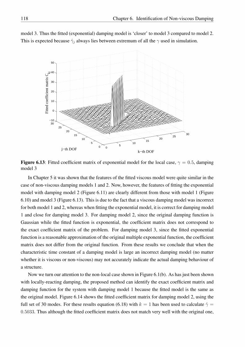
118 Chapter 6. Identification of Non-viscous Damping
model 3. Thus the fitted (exponential) damping model is ‘closer’ to model 3 compared to model 2.This is expected because γj always lies between extremum of all the γ used in simulation.
05
1015
2025
30
0
510
15
2025
30−10
0
10
20
30
40
50
k−th DOFj−th DOF
Fitt
ed c
oeffi
cien
t mat
rix C kj
Figure 6.13: Fitted coefficient matrix of exponential model for the local case, γ = 0.5, dampingmodel 3
In Chapter 5 it was shown that the features of the fitted viscous model were quite similar in thecase of non-viscous damping models 1 and 2. Now, however, the features of fitting the exponentialmodel with damping model 2 (Figure 6.11) are clearly different from those with model 1 (Figure6.10) and model 3 (Figure 6.13). This is due to the fact that a viscous damping model was incorrectfor both model 1 and 2, whereas when fitting the exponential model, it is correct for damping model1 and close for damping model 3. For damping model 2, since the original damping function isGaussian while the fitted function is exponential, the coefficient matrix does not correspond tothe exact coefficient matrix of the problem. For damping model 3, since the fitted exponentialfunction is a reasonable approximation of the original multiple exponential function, the coefficientmatrix does not differ from the original function. From these results we conclude that when thecharacteristic time constant of a damping model is large an incorrect damping model (no matterwhether it is viscous or non-viscous) may not accurately indicate the actual damping behaviour ofa structure.
Now we turn our attention to the non-local case shown in Figure 6.1(b). As has just been shownwith locally-reacting damping, the proposed method can identify the exact coefficient matrix anddamping function for the system with damping model 1 because the fitted model is the same asthe original model. Figure 6.14 shows the fitted coefficient matrix for damping model 2, using thefull set of 30 modes. For these results equation (6.18) with k = 1 has been used to calculate γ =
0.5033. Thus although the fitted coefficient matrix does not match very well with the original one,

6.5. Fitting of the Coefficient Matrix 119
we find once again that the value of the characteristic time constant is quite accurately predicted.For damping model 3 it was observed (results not shown) that, as in the locally-reacting case, theidentified coefficient matrix is very close to the original one.
05
1015
2025
30
0
510
15
2025
30−4
−3
−2
−1
0
1
2
3
4
5
k−th DOFj−th DOF
Fitt
ed c
oeffi
cien
t mat
rix C kj
Figure 6.14: Fitted coefficient matrix of exponential model for the non-local case, γ = 0.5, damp-ing model 2
It might be thought that a useful check on the accuracy of the fitting method could be madeby comparing the ‘measured’ and reconstructed transfer functions. However, little informationis gained from such a comparison. The reason is that, for both viscous and non-viscous fittingprocedures, the poles and corresponding residues of all transfer functions are fitted correctly. Itfollows from Liouville’s theorem that the transfer functions are always well reproduced. Thisdemonstrates that there is a fundamental ambiguity in damping identification: two different damp-ing models (eg., the viscous model and the exponential model) with different spatial distributionsand different sets of parameters can reproduce accurately the full set of transfer functions of asystem with an entirely different damping model (eg., the Gaussian model) with different spatialdistributions and parameters. This in turn implies that just by measuring the transfer functions it is
not possible to identify uniquely the governing damping mechanism. However, it should be notedthat in cases like Figures 6.11, 6.14 etc., the fitted coefficient matrix is not symmetric. This is anon-physical result, which can be regarded as evidence that the true damping behaviour is not infact described by an exponential function. In Chapter 5 similar features were also observed whilefitting a viscous damping matrix.

120 Chapter 6. Identification of Non-viscous Damping
6.6 Conclusions
In this chapter a method has been proposed to identify a non-proportional non-viscous dampingmodel in vibrating systems. It is assumed that damping is light so that the first-order perturbationmethod is applicable. The method is simple, direct, and compatible with conventional modaltesting procedures. The complex modes and natural frequencies are used together with the systemmass matrix. The method does not require the full set of modal data. The damping behaviour isassumed to be described by an exponential relaxation function, and the relaxation time constantis found as part of the fitting procedure. Identification of the familiar viscous damping model is aspecial case of the general method proposed here. The validity of the proposed method has beenexplored by applying it to simulated data from a simple test problem, in which a linear array ofspring-mass oscillators is damped by non-viscous elements over part of its length.
Numerical experiments have been carried out with a wide range of parameter values and dif-ferent damping models. The main features of the results have been illustrated by two particulardamping models and representative parameter values. It has been shown that the method generallypredicts the spatial location of the damping with good accuracy, and also gives a good indication ofwhether the damping is locally-reacting or not. In general, the relaxation time constant was fittedwell, even when the coefficient matrix was less accurate. The transfer functions obtained fromthe fitted exponential damping model agree well with the exact transfer functions of the simulatedsystem. Reciprocity of the transfer functions is preserved within an acceptable accuracy, althoughin some cases the fitted coefficient matrix is not symmetric, indicating that the true damping modeldiffers from the assumed exponential model.
When the time constant is short compared with the periods of all modes retained in the analy-sis, the damping is close to viscous and the fitting procedure gives a physically-sensible symmetriccoefficient matrix and an accurate value of the relaxation parameter. When the time constant islarger, though, the memory of the damping function influences the detailed behaviour. If the iden-tified model matches the true model then the fitting procedure gives a correct physical descriptionof the damping. When the models are different, the poles and residues of the transfer functionsare still fitted accurately with a model of the form considered, but the underlying different func-tional behaviour manifests itself in a non-symmetrical coefficient matrix and significant variationof fitted relaxation parameter with mode number. A correct physical description of the dampingmechanism can be obtained only if a correct model is selected and fitted.
From equation (6.2) we can deduce that, within the approximation of small damping, eachfrequency function G′
kj(ω) can be observed at only two frequencies, ωj and ωk. This fact imposesa fundamental restriction on identification of an exact damping function using this approach. Whenthe fitted coefficient matrix turns out to be non-symmetric, this indicates that it was not possible tofit the assumed function through both ‘measured’ frequency points, and two different coefficientswere needed. To correct this problem it would be necessary to fit a different damping model,

6.6. Conclusions 121
able to pass through both measured points while retaining symmetric coefficients. The functioncannot be uniquely determined by this requirement, of course. There can be two possible ways totackle this problem. One can ‘invent’ different physically plausible damping models and try to fittheir parameters using the approach outlined in this chapter and see which model fits the measureddata most convincingly. Alternatively, one might use the viscous or exponential model and putconstraints on the coefficients such that they yield symmetric coefficient damping matrix. Thisapproach is explored in the next chapter.

122 Chapter 6. Identification of Non-viscous Damping

Chapter 7
Symmetry Preserving Methods forDamping Identification
7.1 Introduction
In the preceding two chapters (Chapter 5 and Chapter 6) methods were proposed to identify viscousand non-viscous damping models from modal data. Some general conclusions emerging from thesestudies are
1. Whenever the fitted damping model (whether viscous or non-viscous) is not close to theoriginal damping model of the system, the identified coefficient matrix becomes asymmetric.
2. Once the poles and residues of transfer functions are obtained, several damping models canbe fitted. In other words, more than one damping model can reproduce some measured setof transfer functions exactly.
An asymmetric fitted damping matrix is a non-physical result because the original system is recip-rocal. Thus, result 1 above may be regarded as an indication of the fact that the selected model isincorrect. Whereas, result 2 indicates that if one’s interest is reconstructing the transfer functionswithin a given frequency band, then it does not matter even if a wrong damping model is assumed.This is the justification of widespread use of the viscous damping model. Motivated by these facts,in this chapter we consider fitting of viscous and exponential damping models so that reciprocityof the system is preserved. Unless the identified damping matrix is symmetric, the model mayhave poor predictive power for changes to the system.
Like the previous two chapters, analysis in this chapter is restricted to linear systems withlight damping. Based on first-order perturbation results, a method for identification of a symmetrypreserving viscous damping model using complex modes and natural frequencies is outlined inSection 7.2. In Section 7.3 this method is extended to identify the coefficients of an exponentialdamping model with a single relaxation parameter. Applications of these methods are illustratedby considering a few numerical examples. Finally Section 7.4 summarizes the main findings ofthis chapter.
123

124 Chapter 7. Symmetry Preserving Methods
7.2 Identification of Viscous Damping Matrix
7.2.1 Theory
In Chapter 5 we have proposed a method to identify a viscous damping matrix from measuredcomplex frequencies and modes using a Galerkin type error minimization approach. This methoddoes not guarantee symmetry of the identified damping matrix. In a numerical simulation study itwas observed that in some cases the identified viscous damping matrix becomes asymmetric. Thisis a non-physical result since the viscous damping matrix by its definition (through the Rayleighsdissipation function) is symmetric. For this reason we now develop a method so that the identi-fied damping matrix is always symmetric. A Lagrange multiplier based constrained optimizationmethod is adopted for this purpose.
Consider λj and zj for all j = 1, 2, · · ·m to be the measured complex natural frequencies andmodes. Here zj ∈ CN where N denotes the number of measurement points on the structure andthe number of modes considered in the study is m. In general m 6= N , usually N ≥ m. Denotethe complex modal matrix
Z = [z1, z2, · · · , zm] ∈ CN×m. (7.1)
If the measured complex mode shapes are consistent with a viscous damping model then fromequation (5.1) the real part of each complex natural frequency gives the undamped natural fre-quency:
ωj = <(λj
). (7.2)
Similarly from equation (5.2), the real part of the complex modes immediately gives the corre-sponding undamped modes and the usual mass orthogonality relationship will be automaticallysatisfied. Write
Z = U + iV (7.3)
where
U = [u1, u2, · · · , um] ∈ RN×m
and V = [v1, v2, · · · , vm] ∈ RN×m(7.4)
are respectively the matrices of real and imaginary parts of the measured complex modes. Now inview of equation (5.2), expand the imaginary part of zj as a linear combination of uj:
vj =m∑
k=1
Bkjuk; where Bkj =ωjC
′kj
ω2j − ω2
k
. (7.5)
The constants Bkj should be calculated such that the error in representing vj by the above sum isminimized while the resulting damping matrix remains symmetric. Note that in the above sum wehave included the k = j term although in the original sum in equation (5.2) this term was absent.This is done to simplify the mathematical formulation to be followed, and has no effect on the

7.2. Identification of Viscous Damping Matrix 125
result. Our interest lies in calculating C ′kj from B′
kj through the relationship given by the secondpart of the equation (7.5), and indeed for k = j we would obtain C ′
kj = 0. The diagonal terms C ′jj
are instead obtained from the imaginary part of the complex natural frequencies:
C ′jj = 2=(λj). (7.6)
For symmetry of the identified damping matrix C, it is required that C′ is symmetric, that is
C ′kj = C ′
jk. (7.7)
Using the relationship given by the second part of the equation (7.5) the above condition reads
Bkj
ω2j − ω2
k
ωj
= Bjk
ω2k − ω2
j
ωk
. (7.8)
Simplification of equation (7.8) yields
Bkj
ωj
= −Bjk
ωk
or Bkjωk + Bjkωj = 0; ∀k 6= j. (7.9)
For further calculations is it convenient to cast the above set of equations in a matrix form. ConsiderB ∈ Rm×m to be the matrix of unknown constants Bkj and define
Ω = diag(ω1, ω2, · · · , ωm) ∈ Rm×m (7.10)
to be the diagonal matrix of the measured undamped natural frequencies. From equation (7.9) forall k, j = 1, 2, · · · ,m (including k = j for mathematical convenience) we have
ΩB + BT Ω = 0 (7.11)
This equation must be satisfied by the matrix B in order to make the identified viscous dampingmatrix C symmetric. The error from representing vj by the series sum (7.5) can be expressed as
εj = vj −m∑
k=1
Bkjuk ∈ RN (7.12)
We need to minimize the above error subject to the constraints given by equation (7.9). Thestandard inner product norm of εj is selected to minimize the error. Considering the Lagrangemultipliers φkj the objective function may be constructed as
χ2 =m∑
j=1
εTj εj +
m∑j=1
m∑
k=1
(Bkjωk + Bjkωj) φkj (7.13)
To obtain Bjk by the error minimization approach set
∂χ2
∂Brs
= 0; ∀r, s = 1, · · · , m. (7.14)

126 Chapter 7. Symmetry Preserving Methods
Substituting εj from equation (7.12) one has
− 2uTr
(vs −
m∑
k=1
Bksuk
)+ [φrs + φsr] ωr = 0
orm∑
k=1
(uT
r uk
)Bks +
1
2[ωrφrs + ωrφsr] = uT
r vs; ∀r, s = 1, · · · ,m.
(7.15)
The above set of equations can be represented in a matrix form as
WB +1
2
[ΩΦ + ΩΦT
]= D (7.16)
where
W =UT U ∈ Rm×m
D =UT V ∈ Rm×m(7.17)
and Φ ∈ Rm×m is the matrix of φrs. Note that both B and Φ are unknown, so there are in total 2m2
unknowns. Equation (7.16) together with the symmetry condition (7.11) provides 2m2 equations.Thus both B and Φ can be solved exactly provided their coefficient matrix is not singular or badlyscaled. We follow the following procedure to obtain B and Φ.
Because in this study Φ is not a quantity of interest, we try to eliminate it. Recalling that Ω isa diagonal matrix taking transpose of (7.16) one has
BT WT +1
2
[ΦT Ω + ΦΩ
]= DT (7.18)
Now postmultiplying equation (7.16) by Ω and premultiplying equation (7.18) by Ω and subtract-ing one has
WBΩ +1
2ΩΦΩ +
1
2ΩΦT Ω− ΩBT WT − 1
2ΩΦT Ω− 1
2ΩΦΩ = DΩ− ΩDT
or WBΩ− ΩBT WT = DΩ− ΩDT .(7.19)
This way Φ has been eliminated. However, note that since the above is a rank deficient system ofequations it cannot be used to obtain B and here we need to use the symmetry condition (7.11).Rearranging equation (7.11) we have
BT = −ΩBΩ−1
(7.20)
Substituting BT in equation (7.19) and premultiplying by Ω−1
results in
Ω−1
WBΩ + ΩBΩ−1
WT = Ω−1
DΩ− DT . (7.21)
Observe from equation (7.17) that W is a symmetric matrix. Now denote
Q =Ω−1
W = Ω−1
WT
P =Ω−1
DΩ− DT .(7.22)

7.2. Identification of Viscous Damping Matrix 127
Using the above definitions, equation (7.21) reads
QBΩ + ΩBQ = P. (7.23)
This matrix equation represents a set of m2 equations and can be solved to obtain B (m2 unknowns)uniquely. To ease the solution procedure let us define the operation vec: Rm×n → Rmn whichtransforms a matrix to a long vector formed by stacking the columns of the matrix in a sequenceone below other. It is known that (see Zhou et al., 1995, page 25) for any three matrices A ∈Ck×m, B ∈ Cm×n, and C ∈ Cn×l, we have vec (ABC) =
(CT ⊗ A
)vec(B) where ⊗ denotes
the Kronecker product. Using this relationship and taking vec of both side of equation (7.23) oneobtains
(Ω⊗Q
)vec(B) +
(QT ⊗ Ω
)vec (B) = vec (P)
or [R] vec (B) = vec (P)(7.24)
where
R =(Ω⊗Q
)+
(QT ⊗ Ω
)∈ Rm2×m2
. (7.25)
Since R is square matrix equation (7.24) can be solved to obtain
vec (B) = [R]−1 vec (P) . (7.26)
From vec (B) the matrix B can be easily obtained by the inverse operation. Obtaining B in sucha way will always make the identified damping matrix symmetric. The coefficients of the modaldamping matrix can be derived from
C ′kj =
(ω2j − ω2
k)Bkj
ωj
; k 6= j (7.27)
Once C′ is obtained, the damping matrix in the original coordinates can be obtained fromequation (5.14). In summary, this procedure can be described by the following steps:
1. Measure a set of transfer functions Hij(ω) at a set of N grid points. Fix the number ofmodes to be retained in the study, say m. Determine the complex natural frequencies λj
and complex mode shapes zj from the transfer function, for all j = 1, · · ·m. Denote Z =
[z1, z2, · · · zm] ∈ CN×m the complex mode shape matrix.
2. Set the ‘undamped natural frequencies’ as ωj = <(λj). Denote the diagonal matrixΩ = diag(ω1, ω2, · · · , ωm) ∈ Rm×m.
3. Separate the real and imaginary parts of Z to obtain U = <[Z
]and V = =
[Z
].
4. From these obtain the m × m matrices W = UT U, D = UT V, Q = Ω−1
W and P =
Ω−1
DΩ− DT .

128 Chapter 7. Symmetry Preserving Methods
5. Now denote p = vec (P) ∈ Rm2
and calculate R =(Ω⊗Q
)+
(QT ⊗ Ω
)∈ Rm2×m2
(MATLABTM command kron can be used to calculate the Kronecker product).
6. Evaluate vec (B) = [R]−1 p and obtain the matrix B.
7. From the B matrix get C ′kj =
(ω2j − ω2
k)Bkj
ωj
for k 6= j and C ′jj = 2=(λj).
8. Finally, carry out the transformation C =
[(UTU
)−1
UT
]T
C′[(
UT U)−1
UT
]to get the
damping matrix in physical coordinates.
A numerical illustration of the proposed method is considered next.
7.2.2 Numerical Examples
Numerical studies have been carried out using simulated systems identical to those used in Chap-ters 5 and 6. Figure 7.1 shows the model systems together with the numerical values used. The
(a)
(b)
m
. . .
. . .
uk uk umuk um uk um uk
umukum
ukumukuk
g(t)
g(t)
g(t)
N- th
N- th
um uk
u
Figure 7.1: Linear array of N spring-mass oscillators, N = 30, mu = 1 Kg, ku = 4× 10³N/m.
damping elements are associated with masses between the s-th and (s + l)-th (N = 30, s = 8 and(s+l) = 17 are taken for the numerical calculations). Damping shown in Figure 7.1(a) is describedas ‘locally reacting’ and that in Figure 7.1(b) is called ‘non-locally reacting’. The dissipative el-ements shown in Figure 7.1 are taken to be linear non-viscous dampers so that the equations ofmotion are described by (5.16). The two damping models considered in Chapter 5 are used. Herewe seek to identify a symmetric viscous damping matrix using the modal data.

7.2. Identification of Viscous Damping Matrix 129
05
1015
2025
30
0
510
15
2025
30−5
0
5
10
15
20
25
k−th DOFj−th DOF
Fitt
ed v
isco
us d
ampi
ng m
atrix
C kj
Figure 7.2: Fitted viscous damping matrix for the local case, γ = 0.02, damping model 2
Results for Small γ
When γ = 0.02 both damping models show near-viscous behaviour. In Section 5.4.1 it was shownthat for this case the fitted viscous damping matrix is symmetric. For this reason, results obtainedby using the symmetry preserving identification procedure developed in this paper must approachto the corresponding results obtained by using the procedure outlined in Chapter 5. Figure 7.2shows the fitted viscous damping matrix for the local case using damping model 2. One immedi-ately recognizes that this result is similar to its corresponding result shown in Figure 5.2. Figure7.3 shows the fitted viscous damping matrix for non-local case using damping model 2. Again, thefitted matrix is similar to its corresponding case shown in Figure 5.5. Thus, when γ is small, theprocure developed in the last section and that outlined in Chapter 5 yields similar result.
Results for Larger γ
When γ is larger the two non-viscous damping models depart from the viscous damping model.For this case, one obtains an asymmetric fitted viscous damping matrix following the procedurein Chapter 5. It is interesting to see how these results change when symmetry preserving methoddeveloped here is applied. Figure 7.4 shows the result of running the symmetry preserving fittingprocedure for damping model 1 with locally-reacting damping and the full set of modes. Theresult of applying the usual viscous damping identification procedure corresponding to this casewas shown before in Figure 5.7. Comparing the Figures 5.7 and 7.4 it may be observed that allthe features of fitting in Figure 5.7, except asymmetry of the damping matrix, reappears in Figure7.4. From the high non-zero values along the diagonal it is easy to identify the spatial location

130 Chapter 7. Symmetry Preserving Methods
05
1015
2025
30
0
510
15
2025
30−30
−20
−10
0
10
20
30
40
50
k−th DOFj−th DOF
Fitt
ed v
isco
us d
ampi
ng m
atrix
C kj
Figure 7.3: Fitted viscous damping matrix for the non-local case, γ = 0.02, damping model 2
of damping. Also observe that all non-zero off-diagonal elements have positive values. Thisimplies that the damping mechanism maybe locally reacting. In order to understand what resultthe symmetry preserving fitting procedure yields when damping is significantly non-viscous weconsider γ = 2 for damping model 1. Figure 7.5 shows the fitted viscous damping matrix for localcase. The result corresponding to this without using the symmetry preserving method was beforeshown in Figure 5.9. Again, from Figure 7.5 the spatial distribution of damping can be guessed,however, the accuracy is reduced as the fitted model differs significantly from the actual dampingmodel.
Figure 7.6 shows the symmetric fitted viscous damping matrix for damping model 2 corre-sponding to the case considered earlier in Figure 5.8. Comparing Figures 5.8 and 7.6, observationssimilar to the case of damping model 1 can be made. Consider now the effect of modal truncationon the symmetry preserving damping identification procedure. In practice, one might hope to beable to use only the first few modes of the system to identify the damping matrix. Figures 7.7 and7.8 shows the fitted viscous damping matrix using, respectively, the first 20 and the first 10 modesonly. The quality of the fitted damping matrix does not significantly deteriorate as the numberof modes used to fit the damping matrix is reduced. This in turn implies that, if the fitted model(viscous in this case) is not close to the original one, then by using more modes in the symmetrypreserving identification method does not significantly improve the result.
Figures 7.9 and 7.10 show the fitted symmetric viscous damping matrix for γ = 0.5 using thenon-local damping model for damping model 1 and 2. Results corresponding to these obtainedwithout the symmetry preserving method was shown in Figures 5.10 and 5.11. The spatial distri-

7.2. Identification of Viscous Damping Matrix 131
05
1015
2025
30
0
510
15
2025
30−1
0
1
2
3
4
5
6
7
8
k−th DOFj−th DOF
Fitt
ed v
isco
us d
ampi
ng m
atrix
C kj
Figure 7.4: Fitted viscous damping matrix for the local case, γ = 0.5, damping model 1
05
1015
2025
30
0
510
15
2025
300
0.2
0.4
0.6
0.8
1
1.2
1.4
1.6
1.8
k−th DOFj−th DOF
Fitt
ed v
isco
us d
ampi
ng m
atrix
C kj
Figure 7.5: Fitted viscous damping matrix for the local case, γ = 2.0, damping model 1
bution of the damping is revealed quite clearly and correctly. In both cases, the non-local natureof the damping is hinted at by the strong negative values on either side of the main diagonal of thematrix.
Because the symmetry preserving method uses a constrained optimization approach, numericalaccuracy of the fitting procedure might be lower compared to the procedure outlined in Chapter 5.

132 Chapter 7. Symmetry Preserving Methods
05
1015
2025
30
0
510
15
2025
30−1
0
1
2
3
4
5
k−th DOFj−th DOF
Fitt
ed v
isco
us d
ampi
ng m
atrix
C kj
Figure 7.6: Fitted viscous damping matrix for the local case, γ = 0.5, damping model 2
05
1015
2025
30
0
510
15
2025
30−1
0
1
2
3
4
5
k−th DOFj−th DOF
Fitt
ed v
isco
us d
ampi
ng m
atrix
C kj
Figure 7.7: Fitted viscous damping matrix using first 20 modes for the local case, γ = 0.5,damping model 2
In order to check numerical accuracy we have reconstructed the transfer functions using the com-plex modes obtained by using the fitted viscous damping matrix. Comparison between a typicaloriginal and reconstructed transfer function Hkj(ω), for k = 11 and j = 24 is shown in Figure7.11, based on locally-reacting damping using damping model 1. It is clear that the reconstructed

7.2. Identification of Viscous Damping Matrix 133
05
1015
2025
30
0
510
15
2025
30−1
0
1
2
3
4
5
k−th DOFj−th DOF
Fitt
ed v
isco
us d
ampi
ng m
atrix
C kj
Figure 7.8: Fitted viscous damping matrix using first 10 modes for the local case, γ = 0.5,damping model 2
0
5
10
15
20
25
30
05
1015
2025
30−2
0
2
4
6
8
k−th DOFj−th DOF
Fitt
ed v
isco
us d
ampi
ng m
atrix
C kj
Figure 7.9: Fitted viscous damping matrix for the non-local case, γ = 0.5, damping model 1
transfer function agrees well with the original one. Thus the symmetry preserving viscous damp-ing matrix identification method developed here does not introduce much error due to the appliedconstrains in the optimization procedure.

134 Chapter 7. Symmetry Preserving Methods
05
1015
2025
30
05
1015
2025
30−1
−0.5
0
0.5
1
1.5
k−th DOFj−th DOF
Fitt
ed v
isco
us d
ampi
ng m
atrix
C kj
Figure 7.10: Fitted viscous damping matrix for the non-local case, γ = 0.5, damping model 2
7.3 Identification of Non-viscous Damping
7.3.1 Theory
As has been mentioned earlier, out of several non-viscous damping models the exponential functionturns out to be the most plausible. In this section we outline a general method to fit an exponentialmodel to measured data such that the resulting coefficient matrix remains symmetric. We assumethat the mass matrix of the structure is known either directly from a finite element model or bymeans of modal updating. Also suppose that the damping has only one relaxation parameter, sothat the matrix of the kernel functions is of the form
G(t) = µe−µt C (7.28)
where µ is the relaxation parameter and C is the associated coefficient matrix. In Chapter 6 amethod was proposed to obtain µ and C from measured complex modes and frequencies. Thismethod may yield a C matrix which is not symmetric. In this section we develop a method whichwill always produce a symmetric C matrix.
The starting point of our discussion is equations (6.12) and (6.13), the expressions for the realand imaginary parts of the complex modes of a linear system with damping of the form (7.28).Assume that
X = [x1, x2, · · · , xm] ∈ RN×m (7.29)
is the matrix of undamped mode shapes and µ is the relaxation parameter and m is the number of
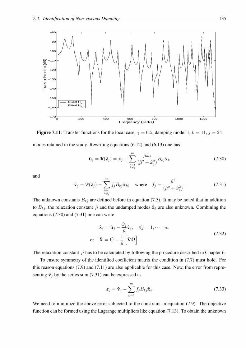
7.3. Identification of Non-viscous Damping 135
0 200 400 600 800 1000 1200−170
−160
−150
−140
−130
−120
−110
−100
−90
−80
Frequency (rad/s)
Tran
sfer F
uncti
on (d
B)
Exact Hk,j
Fitted H
k,j
Figure 7.11: Transfer functions for the local case, γ = 0.5, damping model 1, k = 11, j = 24
modes retained in the study. Rewriting equations (6.12) and (6.13) one has
uj = <(zj) = xj +m∑
k=1k 6=j
µωj
(µ2 + ω2j )
Bkjxk (7.30)
and
vj = =(zj) =m∑
k=1k 6=j
fjBkjxk; where fj =µ2
(µ2 + ω2j )
. (7.31)
The unknown constants Bkj are defined before in equation (7.5). It may be noted that in additionto Bkj , the relaxation constant µ and the undamped modes xk are also unknown. Combining theequations (7.30) and (7.31) one can write
xj = uj − ωj
µvj; ∀j = 1, · · · ,m
or X = U− 1
µ
[VΩ
].
(7.32)
The relaxation constant µ has to be calculated by following the procedure described in Chapter 6.To ensure symmetry of the identified coefficient matrix the condition in (7.7) must hold. For
this reason equations (7.9) and (7.11) are also applicable for this case. Now, the error from repre-senting vj by the series sum (7.31) can be expressed as
εj = vj −m∑
k=1
fjBkjxk (7.33)
We need to minimize the above error subjected to the constraint in equation (7.9). The objectivefunction can be formed using the Lagrange multipliers like equation (7.13). To obtain the unknown
136 Chapter 7. Symmetry Preserving Methods
coefficients Bjk using equation (7.14) one has
− 2xTr
(vs −
m∑
k=1
fsBksxk
)+ + [φrs + φsr] ωr = 0
orm∑
k=1
(xT
r xk
)fsBks +
1
2[ωrφrs + ωrφsr] = xT
r vs; ∀r, s = 1, · · · ,m
(7.34)
The above set of equations can be combined in a matrix form and can be conveniently expressedas
W1BF +1
2
[ΩΦ + ΩΦT
]= D1. (7.35)
where the m×m matrices
W1 =XT X
D1 =XT V
F =diag(f1, f2, · · · , fm).
(7.36)
Equation (7.35) needs to be solved with the symmetry condition (7.11). To eliminate Φ, postmul-tiplying (7.35) by Ω and premultiplying its transpose by by Ω and subtracting we obtain
W1BFΩ− ΩFT BTW1T = D1Ω− ΩD1
T . (7.37)
Substitution of BT from (7.20) in the above equation and premultiplication by Ω−1
results
Ω−1
W1BFΩ + FT ΩBΩ−1
W1T = Ω
−1D1Ω−D1
T . (7.38)
Observe from equation (7.36) that W1 is a symmetric matrix and F is diagonal matrix. Now denote
Q1 =Ω−1
W1 = Ω−1
W1T
P1 =Ω−1
D1Ω−D1T
H =FΩ = FT Ω.
(7.39)
Using above definitions equation (7.38) reads
Q1BH + HBQ1 = P1. (7.40)
This equation is similar to equation (7.23) obtained for the viscously damped case and can besolved using a similar procedure by taking vec of both sides. The procedures to be followed laterto obtain the coefficient matrix C also remain similar to the viscously damped case. In summarythe method can be implemented by the following steps:
1. Measure a set of transfer functions Hij(ω) at a set of N grid points. Fix the number ofmodes to be retained in the study, say m. Determine the complex natural frequencies λj
and complex mode shapes zj from the transfer function, for all j = 1, · · ·m. Denote Z =
[z1, z2, · · · zm] ∈ CN×m the complex mode shape matrix.

7.3. Identification of Non-viscous Damping 137
2. Set the ‘undamped natural frequencies’ as ωj = <(λj). Denote the diagonal matrix Ω =
diag(ω1, ω2, · · · , ωm) ∈ Rm×m.
3. Separate the real and imaginary parts of Z to obtain U = <[Z
]and V = =
[Z
].
4. Obtain the relaxation parameter µ =ω1v
T1 Mv1
vT1 Mu1
.
5. Calculate the diagonal matrix F = diag(
µ2
(µ2+ω2j )
)∈ Rm×m.
6. Obtain the ‘undamped modal matrix’ X = U− 1
µ
[VΩ
].
7. From these evaluate the m×m matrices W1 = XT X, D1 = XT V, Q1 = Ω−1
W1,P1 = Ω
−1D1Ω−D1
T and H = FΩ.
8. Now denote p1 = vec (P1) ∈ Rm2
and calculate R1 = (H⊗Q1)+(Q1
T ⊗H) ∈ Rm2×m2
.
9. Evaluate vec (B) = [R1]−1 p1 and obtain the matrix B.
10. From the B matrix get C ′kj =
(ω2j − ω2
k)Bkj
ωj
for k 6= j and C ′jj = 2=(λj).
11. Finally, carry out the transformation C =
[(XTX
)−1
XT
]T
C′[(
XT X)−1
XT
]to get the
damping matrix in physical coordinates.
7.3.2 Numerical Examples
We again consider the systems shown in Figure 7.1 to illustrate symmetry preserving fitting of ex-ponential damping models outlined in last subsection. Three damping models, given by equations(6.21), (6.21) and (6.23) will be considered. Recall that the relaxation parameter has to be obtainedby the procedure outlined in Chapter 6. So here we will only discuss fitting of the coefficient ma-trix.
Results for Small γ
It has been mentioned before that when γ is small, the ordinary viscous damping identificationmethod (in Chapter 5), non-viscous damping identification method (in Chapter 6) and symmetrypreserving viscous damping identification method (in Section 7.2) yields same result. This isbecause all the non-viscous damping models approach to a viscous damping model for small valueof γ. Since the viscous damping model is a special case of the exponential damping model, weexpect this method to produce results like the three previous methods. Figure 7.12 shows the fittedcoefficient matrix of the exponential model for damping model 2, calculated using the complete setof 30 modes. It is clear that this result is similar to the corresponding result obtained in Figure 6.8

138 Chapter 7. Symmetry Preserving Methods
without using the symmetry preserving method. Figure 7.13 shows the fitted coefficient matrix fordamping model 2 for the non-local case using the symmetry preserving method. Again, comparingit with Figure 6.9 one observes that they are similar. Thus, when γ is small the symmetry preservingmethod for fitting the coefficient matrix for the exponential function and the method described inChapter 6 yields similar results.
05
1015
2025
30
0
510
15
2025
30−5
0
5
10
15
20
25
30
k−th DOFj−th DOF
Fitt
ed c
oeffi
cien
t mat
rix C kj
Figure 7.12: Fitted coefficient matrix of exponential model for the local case, γ = 0.02, dampingmodel 2
Results for Larger γ
When γ is larger the two non-exponential damping models depart from the exponential dampingmodel. Like previous examples, we consider γ = 0.5. For this case, in Chapter 6 it was observedthat the identification method proposed there results an asymmetric coefficient matrix. The degreeof asymmetry of the fitted coefficient depends on how much the original damping model deviatesfrom the identified exponential model. Specifically, it was concluded that if variation of µj withj calculated using equation (6.17) is more, then the fitted coefficient matrix is likely to be moreasymmetric. In this section we want to understand how the proposed method overcomes thisproblem and what one could tell from the identified coefficient matrix about the nature of damping.Figure 7.14 shows the fitted symmetric coefficient matrix for the local case with damping model2. The result corresponding to this without using the symmetry preserving method was shownbefore in Figure 6.11. Comparison of these two figures clearly demonstrates the advantage of theproposed symmetry preserving method. The identified coefficient matrix is not only symmetric,but also the correct spatial location of damping can be deduced from the peak along the diagonal.

7.3. Identification of Non-viscous Damping 139
05
1015
2025
30
0
510
15
2025
30−30
−20
−10
0
10
20
30
40
50
60
k−th DOFj−th DOF
Fitt
ed c
oeffi
cien
t mat
rix C kj
Figure 7.13: Fitted coefficient matrix of exponential model for the non-local case, γ = 0.02,damping model 2
Besides, predominantly positive values of the off-diagonal entries of the fitted coefficient matrixindicate that damping is locally reacting.
05
1015
2025
30
0
510
15
2025
30−1
0
1
2
3
4
5
6
7
8
9
k−th DOFj−th DOF
Fitt
ed c
oeffi
cien
t mat
rix C kj
Figure 7.14: Fitted coefficient matrix of exponential model for the local case, γ = 0.5, dampingmodel 2
To demonstrate the efficacy of the proposed method we consider a further larger value of γ.

140 Chapter 7. Symmetry Preserving Methods
Figure 7.15 shows the fitted coefficient matrix of the exponential function without using the sym-metry preserving method for damping model 2 with γ = 2.0 and local case. Clearly, the largevariation of µj with j, shown in Figure 7.16, is the reason for significant asymmetry of the fittedcoefficient matrix. Application of the symmetry preserving method for this case is shown in Fig-ure 7.17. In spite of large off-diagonal activity one can still guess about the position of damping.Again, like Figure 7.14, non-negative values of the off-diagonal entries indicate that damping is oflocal type.
0
5
10
15
20
25
30
0
5
10
15
20
25
30−0.5
0
0.5
1
1.5
2
2.5
k−th DOFj−th DOF
Fitt
ed c
oeffi
cien
t mat
rix C kj
Figure 7.15: Fitted coefficient matrix of exponential model without using the symmetry preservingmethod for the local case, γ = 2.0, damping model 2
The fitted coefficient matrix for the local case with a double exponential damping model (model3) with γ = 0.5 using the procedure outlined in Chapter 6 was shown in Figure 6.13. Observe thatthis matrix is not asymmetric as the corresponding variation of µj with j, shown in Figure 6.6,is small. Thus, application of the symmetry preserving method will not be significantly differentfrom the result obtained using the procedure in Chapter 6 and may be verified from Figure 7.18.
Finally we turn our attention to the non-local case. Figure 7.19 shows the fitted coefficientmatrix for non-local case with damping model 2 and γ = 0.5. Again, improvement of the fittedcoefficient matrix may be observed by comparing it with Figure 6.14.
7.4 Conclusions
In this chapter a method is proposed to preserve symmetry of the identified damping matrix. Bothviscous and non-viscous damping models are considered. For fitting a viscous damping model

7.4. Conclusions 141
0 5 10 15 20 25 3010
0
1010
1020
1030
1040
1050
Mode number
Ori
gina
l and
fitte
d γ
Fitted γ for different modes Fitted using Eq. (6.19), γ
fit= 31.8381
Fitted using Eq. (6.20), γfit
= 2.7673
Original γ = 2
Figure 7.16: Values of γ obtained from different µ calculated using equations (6.18)–(6.20) forthe local case, damping model 2
05
1015
2025
30
0
5
10
15
20
25
30−0.5
0
0.5
1
1.5
2
2.5
k−th DOFj−th DOF
Fitt
ed c
oeffi
cien
t mat
rix C kj
Figure 7.17: Fitted coefficient matrix of exponential model using the symmetry preserving methodfor the local case, γ = 2.0, damping model 2
only complex natural frequencies and mode shapes are required. To fit a non-viscous model, inaddition to the modal data, knowledge of the mass matrix is also required. However, availabilityof the complete set of modal data is not a requirement of these methods. The proposed methodsutilize a least-square error minimization approach together with a set of constraints which guaran-

142 Chapter 7. Symmetry Preserving Methods
05
1015
2025
30
0
510
15
2025
30−10
0
10
20
30
40
50
k−th DOFj−th DOF
Fitt
ed c
oeffi
cien
t mat
rix C kj
Figure 7.18: Fitted coefficient matrix of exponential model for the local case, γ = 0.5, dampingmodel 3
05
1015
2025
30
0
5
10
15
20
25
30−3
−2
−1
0
1
2
3
4
5
k−th DOFj−th DOF
Fitt
ed c
oeffi
cien
t mat
rix C kj
Figure 7.19: Fitted coefficient matrix of exponential model for the non-local case, γ = 0.5, damp-ing model 2
tee symmetry of the fitted damping matrix. It was shown that, for the cases when application ofthe usual damping identification methods described in Chapters 5 and 6 produces an asymmetricmatrix, this method not only fits a symmetric matrix but also all the other useful information aboutthe systems damping properties are preserved.

Chapter 8
Experimental Identification of Damping
8.1 Introduction
In the last three Chapters several methods have been proposed to identify damping in a vibratingstructure. The purpose of this Chapter is to verify some of the developed theories by conductingvibration experiments. Unlike mass and stiffness properties, damping is a purely dynamic propertyof a system, i.e., damping can be measured only by conducting dynamic testing on a structure.
A description of a mechanical structure requires knowledge of the geometry, boundary condi-tions and material properties. The mass and stiffness matrices of a structure with complicatedgeometry, boundary conditions and material properties can be obtained experimentally or nu-merically (for example, using the finite-element method). Unfortunately, present knowledge ofdamping does not allow us to obtain the damping matrix like the mass and stiffness matrices forcomplicated systems. For this reason we consider simple systems for which geometry, boundaryconditions and material properties are easy to determine. Specifically, a free-free uniform beam inbending vibration is considered in this Chapter to implement and verify the damping identificationprocedures developed so far in this dissertation. Details of the beam experiment will follow inSection 8.3.
The damping identification procedures developed in Chapters 5, 6 and 7 rely on complex natu-ral frequencies and mode shapes. For lightly damped structures, complex natural frequencies canbe expressed in terms of undamped natural frequencies and modal Q-factors. Natural frequencies,Q-factors and mode shapes are collectively called modal parameters or modal data. It should benoted that, in the context of general multiple-degree-of-freedom systems, these modal parameterscan not be directly measured by conducting a vibration experiment. Typically one measures timehistories of the responses at different degrees of freedom together with time histories of the inputforces. The transfer functions of a system can be obtained by taking ratios of Fourier transforms ofoutput time histories to that of corresponding input time histories. The modal parameters of a struc-ture can be extracted from a set of transfer functions obtained in this way. The subject which dealswith extraction of modal parameters is called experimental modal analysis. We refer to the booksby Ewins (1984) and Maia and Silva (1997) for further details on experimental modal analysis. It
143

144 Chapter 8. Experimental Identification of Damping
should be mentioned that the underlying theory behind experimental modal analysis explicitly orimplicitly assumes that damping is viscous. It is legitimate to ask the question: what happens if thedamping of the system is not viscous – does the conventional experimental modal analysis method-ology extract correct modal parameters? In the next section we address this question and proposea generic method to extract modal parameters of generally damped multiple-degrees-of-freedomlinear systems.
8.2 Extraction of Modal Parameters
It was mentioned that the starting point of extracting modal parameters is transfer functions. Atransfer function Hjn(ω) is defined as
Hjn(ω) =uj(ω)
fn(ω)(8.1)
where uj(ω) is the response at j-th degree of freedom and fn(ω) is the applied force at n-th degreeof freedom. A closed-form exact expression of the transfer function matrix of a generally dampedN -degrees-of-freedom linear systems was obtained in Section 3.3. Taking the jn-th element of thetransfer function matrix given by equation (3.65) one has
Hjn(ω) =N∑
k=1
[Rkjn
iω − sk
+R∗
kjn
iω − s∗k
]+
m∑j=2N+1
Rkjn
iω − sk
. (8.2)
In the above expression Rkjnis the jn-th element of the residue matrix corresponding to pole sk.
From equation (3.64) one obtains the relationship between residues Rkjnand mode shapes as
Rkjn= γkznkzjk (8.3)
where znk is the n-th element of k-the mode shape and γk, the normalization constant of k-th mode,was defined in equation (3.66). The poles are related to natural frequencies λk by
sk = iλk. (8.4)
In Chapter 3 it was mentioned that the first part of the right hand side of equation (8.2) corre-sponds to elastic modes and the second part corresponds to non-viscous modes. In general, elasticmodes are complex in nature as damping is non-proportional. For an N -degree-of-freedom linearsystem, N elastic modes together with their complex conjugates correspond to N physical vibra-tion modes. For lightly damped systems, the complex natural frequencies corresponding to theelastic modes have the form
λk ≈ ωk + iωk
2Qk
. (8.5)
In the above equation ωk is the k-th undamped natural frequency and Qk is the k-th Q-factor. TheQ-factors or quality factors, reciprocal of twice the damping ratios, are expressed as
Qk ≈ <(λk)
2=(λk)=
1
2ζk
(8.6)

8.2. Extraction of Modal Parameters 145
where ζk are damping ratios. If the damping is sufficiently light then all the elastic modes are sub-critically damped, i.e., all of them are oscillatory in nature. In this case the transfer functions ofa system has ‘peaks’ corresponding to all the elastic modes. The natural frequencies (ωk) and theQ-factors (Qk) can be obtained by examining each peak separately, for example using the circlefitting method (see Ewins, 1984). Estimation of ωk and Qk is likely to be good if the peaks arewell separated.
For passive systems, the kind of systems we mostly encounter in practice, non-viscous modesare usually over-critically damped. Thus, in contrast to elastic modes, they do not produce anypeaks in the transfer functions. As a consequence to this, the modal parameters correspondingto non-viscous modes cannot be obtained by usual techniques of experimental modal analysis asdiscussed above. This is the fundamental difficulty in applying conventional experimental modalanalysis procedure to non-viscously damped systems. However, as shown through an examplein Section 3.7.1, the non-viscous part of the response may be quite small compared to that ofthe elastic part. Thus, for practical purposes the second part of the right hand side of equation(8.2) may be neglected. In that case, the transfer functions of generally damped systems can berepresented in way similar to viscously damped systems, that is,
Hjn(ω) ≈N∑
k=1
[Rkjn
iω − sk
+R∗
kjn
iω − s∗k
]. (8.7)
Once equation (8.7) is assumed as the expression for transfer functions, conventional exper-imental modal analysis procedure may be applied to deal with non-viscously damped systems.This, analysis justifies that the conventional experimental modal analysis procedure, which a pri-
ori assumes the viscous damping model, indeed measures modal parameters of a system evenwhen it is non-viscously damped. Next, assuming the validity of equation (8.7) a linear-nonlinearoptimization approach is presented to extract complex modal parameters of non-viscously dampedmultiple-degrees-of-freedom linear systems.
8.2.1 Linear Least-Square Method
From equation (8.7) it is easy to observe that Hjn(ω) is a linear function of the residues while it isa nonlinear function of the poles. On the basis of this fact, it is legitimate to separate the extractionprocedure for the poles and the residues. We propose a linear least-square approach to obtain theresidues and a non-linear optimization approach to obtain the poles. Recently Duffour (1998) hasproposed a similar method by considering all the residues to be real. His approach is equivalent toassuming that the systems is proportionally damped and consequently it yields real normal modes.In this section we extend this method to identify complex residues in order to extract complexmodes.
Depending on what quantity is measured, the transfer functions can be (a) displacement trans-fer functions (receptance), (b) velocity transfer functions (mobility), and (c) acceleration transfer

146 Chapter 8. Experimental Identification of Damping
functions (accelerance). Substituting sk from equation (8.4), in a more general form, the transferfunctions given by equation (8.7) may be expressed as
Hjn(ω) ≈ (iω)r
N∑
k=1
[Rkjn
iω − iλk
+R∗
kjn
iω + iλ∗k
]
= (iω)r
N∑
k=1
[− iRkjn
ω − λk
+
(iRkjn
)∗ω + λ∗k
] (8.8)
where
• r = 0 corresponds to displacement transfer functions
• r = 1 corresponds to velocity transfer functions
• r = 2 corresponds to acceleration transfer functions.
Since the systems we consider are reciprocal, the transfer function matrix and consequently theresidue matrix corresponding to each pole is symmetric, that is Rkjn
= Rknj. For this reason
evaluation of the upper or lower half of the transfer function matrix is sufficient. However, mostoften only one row of the transfer matrix is measured in practice. For example, if one uses animpulse hammer for the excitation, then often the response measurement point is kept fixed whilethe excitation point varies according to an a priori selected grid on a structure. Thus, in equation(8.8) , j is fixed with its value equals to the degree of freedom of the response measurement point.Suppose the number of channels (i.e., DOF of the system) is N and the number of modes retainedin the study is m. Usually m ≤ N . For brevity, omitting the subscript j, from equation (8.8) weobtain
Hn(ω) ≈m∑
k=1
[f1k(ω)Akn + f2k
(ω)A∗kn] ; ∀n = 1, 2, · · · , N (8.9)
where
f1k(ω) = − (iω)r
ω − λk
(8.10)
f2k(ω) =
(iω)r
ω + λ∗k(8.11)
Akn = iRkjn. (8.12)
8.2.2 Determination of the Residues
Suppose Yn(ω),∀n = 1, 2, · · · , N are set of the measured transfer functions corresponding toall the channels. We assume that initial estimates of ωk, Qk,∀ k = 1, 2, · · · , m are known, forexample using a circle fitting method. Thus, from equations (8.5), (8.10) and (8.11) it is clear thatthe complex functions f1k
(ω) and f2k(ω) are known for all ω. Our aim is to obtain the matrix
A : Akn ∈ Cm×N such that the error in representing Yn(ω) by equation (8.9) is minimized.

8.2. Extraction of Modal Parameters 147
We define the frequency dependent error as
εn(ω) = Yn(ω)−Hn(ω). (8.13)
Based on this, further define the merit function as
χ2 =N∑
n=1
∫
ω∈Ω
|εn(ω)|2dω
=N∑
n=1
∫
ω∈Ω
εn(ω)ε∗n(ω)dω
(8.14)
where Ω is the range of frequency over which the transfer functions are obtained. To obtain Akn
by the error minimization approach, set
∂χ2
∂Apq
= 0; ∀p = 1, · · · ,m; q = 1, · · · , N. (8.15)
Substituting εn from equation (8.13) the preceding equation can be expressed as
−N∑
n=1
∫
ω∈Ω
[∂Hn(ω)
∂Apq
Y ∗n (ω)−H∗
n(ω)+ Yn(ω)−Hn(ω) ∂H∗n(ω)
∂Apq
]dω = 0. (8.16)
Now, from the expression of Hn(ω) in equation (8.9) one obtains the following:
∂Hn(ω)
∂Apq
= 0; ∀n 6= q (8.17)
∂Hq(ω)
∂Apq
= f1p(ω) (8.18)
∂H∗q (ω)
∂Apq
= f ∗2p(ω). (8.19)
Using the above three equations, (8.16) may be simplified to∫
ω∈Ω
[f1p(ω)H∗
q (ω) + f ∗2p(ω)Hq(ω)
]dω =
∫
ω∈Ω
[f1p(ω)Y ∗
q (ω) + f ∗2p(ω)Yn(ω)
]dω. (8.20)
Substituting the expression of Hn(ω) in (8.9) for n = q, the preceding equation reduces to
m∑
k=1
WpkAkq + EpkA∗kq = Spk (8.21)
where
Wpk =
∫
ω∈Ω
[f1p(ω)f ∗2k
(ω) + f ∗2p(ω)f1k
(ω)]dω (8.22)
Epk =
∫
ω∈Ω
[f1p(ω)f ∗1k
(ω) + f ∗2p(ω)f2k
(ω)]dω (8.23)
Spk =
∫
ω∈Ω
[f1p(ω)Y ∗
q (ω) + f ∗2p(ω)Yn(ω)
]dω. (8.24)

148 Chapter 8. Experimental Identification of Damping
For p = 1, · · · ,m and q = 1, · · · , N equation (8.21) can be rewritten in matrix form as
WA + EA∗ = S (8.25)
where W, E ∈ Cm×m and S ∈ Cm×N . Since χ2 is a real function we also have
∂χ2
∂A∗pq
=
(∂χ2
∂Apq
)∗. (8.26)
In view of the above, taking the complex conjugate of (8.25) one has
W∗A∗ + E∗A = S∗
or A∗ = W∗−1
[S∗ − E∗A](8.27)
Substituting A∗ from the above equation in (8.25) we finally obtain
A =[W− EW∗−1E∗
]−1 [S− EW∗−1S∗
]. (8.28)
Transfer function residues can be calculated from the above formula provided the matrix
W− EW∗−1E∗ 6= Om (8.29)
where Om is a m×m null matrix. Premultiplying the above equation by E−1 and defining
Q = E−1W (8.30)
the condition for which A can be determined can be expressed as
Q 6= Q∗−1
or Q∗Q 6= Im. (8.31)
Determination of the Complex Modes
Once the residues are obtained from equation (8.28), the complex modes can be calculated easily.Combining equations (8.12) and (8.3) one has
Akn = iγkznkzjk. (8.32)
In Chapter 4 it was mentioned that the normalization constants can be selected in various ways.The one which is consistent with conventional modal analysis is when γk = 1/2iλk. Substitutingthis value of γk, equation (8.32) reads
Akn =znkzjk
2λk
. (8.33)
Note that in the above equation j is fixed (the response measurement point). For n = j, fromequation (8.33) one has
zjk =√
2λkAkj; ∀k = 1, 2, · · · ,m (8.34)

8.2. Extraction of Modal Parameters 149
Substituting zjk from the above into equation (8.33) the mode shapes are obtained as
znk =2λkAkn
zjk
=√
2λkAkn√Akj
, ∀ k = 1, 2, · · · ,m,n = 1, 2, · · · , N.
(8.35)
Thus, equation (8.35) together with (8.28), provides a closed-form expression for the complexmodes extracted from a set of measured transfer functions.
8.2.3 Non-linear Least-Square Method
In the formulation presented before it was assumed that ‘good’ initial guesses of ωk and Qk areavailable. However, if substantially good initial values of ωk and Qk are not available then it is re-quired to update them. Since Hn(ω) is a nonlinear function of ωk and Qk, a nonlinear optimizationmethod needs to be employed for this purpose. We use a nonlinear least-square method outlinedin Press et al. (1992, Section 15.5).
For convenience construct the parameter vector
V = ω1, ω2, · · · , ωm, Q1, Q2, · · · , QmT ∈ R2m. (8.36)
Suppose, for some current value of V , say Vcur, χ2(V) is sufficiently close to minimum. Expandingχ2(V) about Vcur in a Taylor series and retaining quadratic terms we have
χ2(V) ≈ χ2(V − Vcur)− (V − Vcur)T ∇χ2 (Vcur) +
1
2(V − Vcur)
T D (V − Vcur) (8.37)
where ∇(•) =
∂(•)∂Vj
, ∀j is the gradient vector and D ∈ R2m×2m is the Hessian matrix. Differ-
entiating equation (8.37) one obtains
∇χ2(V) = ∇χ2 (Vcur) + D (V − Vcur) . (8.38)
If the approximation is good, then by setting ∇χ2(V) = 0, the minimizing parameters Vmin canobtained from the current trial parameters Vcur as
Vmin = Vcur + D−1[−∇χ2 (Vcur)
]. (8.39)
However, if (8.37) is a poor approximation, then the best we can do is to move down the gradient(steepest descent method), that is
Vnext = Vcur − constant×∇χ2 (Vcur) (8.40)
Selection procedure of this constant will be discussed shortly. In order to use (8.39) or (8.40) weneed to calculate the gradient of χ2. Moreover, to use (8.39) calculation of the second derivativematrix (Hessian matrix) is also required. These issues are discussed next.
150 Chapter 8. Experimental Identification of Damping
Calculation of the Gradient and Hessian
Differentiating the expression of χ2 in equation (8.14) with respect to Vp the elements of the gra-dient vector can be obtained as
∂χ2
∂Vp
=N∑
n=1
∫
ω∈Ω
[∂εn(ω)
∂Vp
ε∗n(ω) + εn(ω)∂ε∗n(ω)
∂Vp
]dω
= −N∑
n=1
∫
ω∈Ω
[∂Hn(ω)
∂Vp
ε∗n(ω) + εn(ω)∂H∗
n(ω)
∂Vp
]dω.
(8.41)
The preceding equation can further be simplified as
∂χ2
∂Vp
= −2N∑
n=1
∫
ω∈Ω
<[εn(ω)
∂H∗n(ω)
∂Vp
]dω. (8.42)
The term∂H∗
n(ω)
∂Vp
can be calculated following Appendix A. Taking an additional partial derivative
of (8.41) with respect to Vq the elements of the Hessian matrix can be obtained as
∂2χ2
∂Vp∂Vq
= −N∑
n=1
∫
ω∈Ω
[∂2Hn(ω)
∂Vp∂Vq
ε∗n(ω) +∂Hn(ω)
∂Vp
∂ε∗n(ω)
∂Vq
+∂εn(ω)
∂Vq
∂H∗n(ω)
∂Vp
+ εn(ω)∂2H∗
n(ω)
∂Vp∂Vq
]dω.
(8.43)
Substituting εn from equation (8.13) the preceding equation can be expressed as
∂2χ2
∂Vp∂Vq
= 2N∑
n=1
∫
ω∈Ω
<[∂Hn(ω)
∂Vp
∂H∗n(ω)
∂Vq
− εn(ω)∂2H∗
n(ω)
∂Vp∂Vq
]dω. (8.44)
It is customary to neglect the second term in the above expression because εn(ω) and∂2H∗
n(ω)
∂Vp∂Vq
are
both small quantities. Thus, the elements of the Hessian matrix can be obtained from
∂2χ2
∂Vp∂Vq
≈ 2N∑
n=1
∫
ω∈Ω
<[∂Hn(ω)
∂Vp
∂H∗n(ω)
∂Vq
]dω. (8.45)
For convenience, removing the factors 2 from equations (8.42) and (8.45) we define a vector β ∈R2m and a matrix α ∈ R2m×2m such that
βp = −1
2
∂χ2
∂Vp
(8.46)
αpq =1
2
∂2χ2
∂Vp∂Vq
. (8.47)
The matrix α =1
2D is often known as the curvature matrix. Using these relationships, equation
(8.39) can be rewritten as the set of linear equations
α δV = β. (8.48)
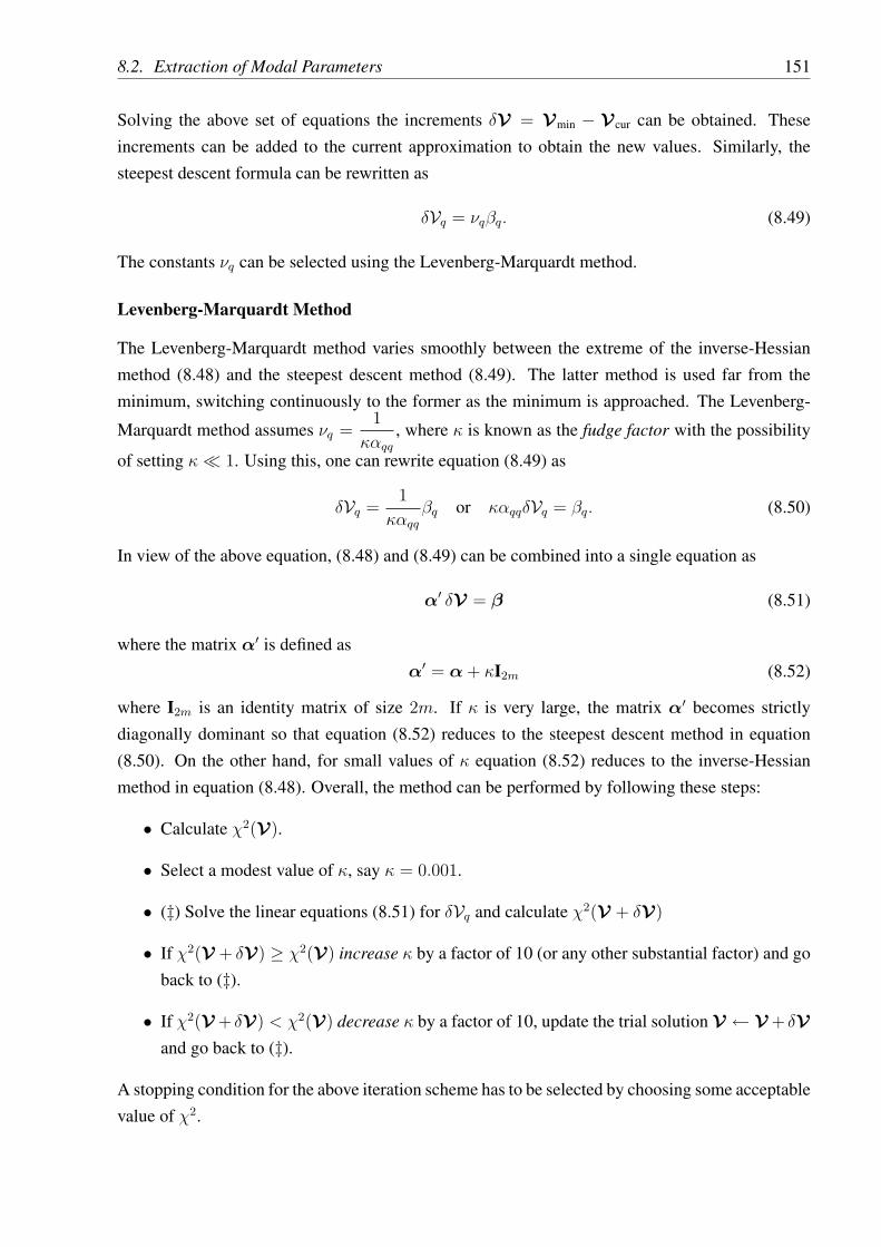
8.2. Extraction of Modal Parameters 151
Solving the above set of equations the increments δV = Vmin − Vcur can be obtained. Theseincrements can be added to the current approximation to obtain the new values. Similarly, thesteepest descent formula can be rewritten as
δVq = νqβq. (8.49)
The constants νq can be selected using the Levenberg-Marquardt method.
Levenberg-Marquardt Method
The Levenberg-Marquardt method varies smoothly between the extreme of the inverse-Hessianmethod (8.48) and the steepest descent method (8.49). The latter method is used far from theminimum, switching continuously to the former as the minimum is approached. The Levenberg-
Marquardt method assumes νq =1
καqq
, where κ is known as the fudge factor with the possibility
of setting κ ¿ 1. Using this, one can rewrite equation (8.49) as
δVq =1
καqq
βq or καqqδVq = βq. (8.50)
In view of the above equation, (8.48) and (8.49) can be combined into a single equation as
α′ δV = β (8.51)
where the matrix α′ is defined as
α′ = α + κI2m (8.52)
where I2m is an identity matrix of size 2m. If κ is very large, the matrix α′ becomes strictlydiagonally dominant so that equation (8.52) reduces to the steepest descent method in equation(8.50). On the other hand, for small values of κ equation (8.52) reduces to the inverse-Hessianmethod in equation (8.48). Overall, the method can be performed by following these steps:
• Calculate χ2(V).
• Select a modest value of κ, say κ = 0.001.
• (‡) Solve the linear equations (8.51) for δVq and calculate χ2(V + δV)
• If χ2(V + δV) ≥ χ2(V) increase κ by a factor of 10 (or any other substantial factor) and goback to (‡).
• If χ2(V + δV) < χ2(V) decrease κ by a factor of 10, update the trial solution V ← V + δVand go back to (‡).
A stopping condition for the above iteration scheme has to be selected by choosing some acceptablevalue of χ2.
152 Chapter 8. Experimental Identification of Damping
8.2.4 Summary of the Method
In the last two sections a linear least-square and a nonlinear least-square method have been pro-posed to obtain the modal parameters. For practical purposes these two methods can unified toconstruct a single linear-nonlinear optimization method. Figure 8.1 shows the steps to followedin order to apply this method. A set of MATLABTM programs have been developed to implementthis method. Several authors, for example Balmes (1995), Cole et al. (1995), Lin and Ling (1996),Balmes (1996) and Rosa et al. (1999) have proposed modal identification methods in frequencydomain. Application of the approach developed in this study to a beam in bending vibration isconsidered next.
Amplitude coefficients [A] computation by linearleast square
Input: ωω, Q, ε
Computation of χ2(ωω, Q, [A])
Computation of the frequencies and dampingincrements: dωω, dQ
Computation of χ2(ωω+dωω, Q+ dQ, [A])
|χ2(ωω+dωω, Q+ dQ, [A])-χ2(ωω, Q, [A])|< ε
Yes
No
Solution displayed
linear
non-linear
Figure 8.1: The general linear-nonlinear optimization procedure for identification of modal pa-rameters

8.3. The Beam Experiment 153
8.3 The Beam Experiment
We consider a free-free beam for experimental verification of the procedures developed so far inthis dissertation. The physical properties of the beam, the arrangement of the damping mechanismand the scheme for the grid points will be discussed in Section 8.3.2. In the next section, the detailsof the equipment used for the experiment are explained.
8.3.1 Experimental Set-up
A schematic diagram of the experimental set-up is shown in Figure 8.2 while the details of themeasuring equipment are given in Table 8.1. Figure 8.2 shows three main components of themeasurement technique implemented:
• Excitation of the structure
• Sensing of the response
• Data acquisition and processing
Details of the above components of the experiment are discussed next.
Excitation of the Structure
A mechanical structure can be excited mainly in two ways, (a) using an exciter or shaker, and(b) using an impulse hammer. Shaker attachments have the advantage of providing any knownwaveform as the driving signal to a structure. This allows one to control the frequency content ofthe excitation and consequently to excite the modes in a chosen frequency-band. In addition, thesteady-state sinusoidal driving is probably the only efficient way to measure the frequency responseat different frequencies directly. However, a major disadvantage of attaching shakers as the drivingmechanism is that it becomes a part of the vibrating structure and as a result the stiffness, and moreimportantly the damping behaviour, which we want to identify from this experiment, get changed.Beside this, there are some practical difficulties, for example:
• it not always convenient to mount a shaker to access all the excitation points we choose;
• to obtain a set of transfer functions with high frequency resolution and covering severalmodes is very time consuming.
For these reasons, the possibility of using shakers has been ruled out for this experiment.It is much easier to excite a structure by hitting it with an instrumented hammer. The instru-
mented hammer essentially consists of three main components: a handle, a force transducer and ahammer tip. With experience it was found that the impulse excitation provided by an instrumentedhammer gave the most reliable results for the present purpose. Impulse excitation using a hammerhas the following advantages:

154 Chapter 8. Experimental Identification of Damping
• the location of excitation point can be chosen arbitrarily;
• once an impulse has been struck and the hammer separated, the response obtained thereafteris free from any undesirable interaction with the excitation apparatus;
• depending on the nature of the hammer tip (that is soft or hard) the frequency range can beselected as desired.
For the hammer used in this experiment, the force transducer was a PCB A218 and a hard plastictip was used. With this hard plastic tip we can go up to 2.5KHz.
Sensing of the Response
Response sensors have to be selected on the basis of what quantity one wants to measure and thesize of the structure under test. The relative size and mass of the response transducers have influ-ence on the vibrational behaviour of the test structure. It is very much desirable that a transducerhas minimum effect on the structure so that one can avoid the corrections required at a later stageto discard the effect of the transducer.
The response of a structure may be defined in terms of displacement, velocity or accelera-tion. Accelerometers are the most widely used form of response transducer although, as laservibrometers are more readily available, velocity transducers are also gaining popularity. The mainadvantage of the laser vibrometer is that the response measurement technique is ‘non-contact’.Thus, questions of interactions between the response measurement apparatus and the structure donot arise for laser vibrometers. Beside, laser vibrometers can be used to measure response at pointswhere accelerometers can not be attached. However, for the simple beam considered in this exper-iment it was found that traditional piezoelectric accelerometers are sufficient. A DJB piezoelectricaccelerometer is used for the experiment. We have measured the acceleration response at onlyone point in the structure (detail will follow in Section 8.3.2). A small hole of 3mm diameter wasdrilled into the beam and the accelerometer was attached by screwing it through the hole.
Data Acquisition and Processing
(a) Amplifiers
Signals from the impulse hammer and the accelerometer give small charges. As a result thesignals need to be amplified by using a charge amplifier. For this purpose in-house charge am-plifiers were designed. The acceleration signal was amplified by using a charge amplifier with asensitivity of 14mV/pc while the impulse signal was amplified by using a charge amplifier with asensitivity of 2.0mV/pc. Both these amplifiers had a frequency range of 0.44Hz to 10KHz.(b) Data-logging system
A National Instruments DAQCard 1200 was used to log the impulse force and the accelerationresponse. This card gives analog-to-digital conversion in 12 bits. The maximum sampling rate wasset to 20kHz, which was sufficient for the frequency bandwidth of interest (i.e., 0-2.5KHz).

8.3. The Beam Experiment 155
beamdamped
computer with A/D card
oscilloscope
output charge amplifier
input charge amplifier
hammer
Figure 8.2: Schematic representation of the test set-up
A Visual Basic program running on a Daytek desktop computer controlled the DAQCard. Thisprogram was used to start data logging, set sampling frequencies, check sample saturation and savethe data. After the raw data were measured and saved they were then opened using MATLABTM andchecked as to whether they were suitable or not by calculating the FRFs.
Item UseDJB Accelerometers Measuring the acceleration
response of the beamPCB modal hammer Measuring the force ap-
plied using the impulsehammer
Impulse charge amplifier Amplifying the impulseforce exerted on the struc-ture
Response charge amplifier Amplifying the accelera-tion response
National Instruments DAQ-Card 1200 data acquisitionpersonal computer card
Sampling transducer timesignals
Daytek Desktop Computer Control of DAQCard 1200,data storage and analysis
Table 8.1: Summary of the equipment used
8.3.2 Experimental Procedure
A steel beam with uniform rectangular cross-section is considered for the experiment. Figure 8.3shows the beam with details of the grid and damping mechanism. The physical and geometricalproperties of the steel beam are shown in Table 8.2. The damping mechanism of the beam isthrough constrained layers (see Ungar, 2000, for a recent review on this topic). For the purpose ofthis experiment a double sided glued tape is sandwiched between the beam and a thin aluminumplate.
The impulse hammer test is performed on the ‘front side’ of the beam (i.e., opposite to thedamping layer side). The impulse is applied at 11 different locations as indicated in Figure 8.3(a).One of the problems that was encountered during impulse testing has the difficulty of exciting thebeam only in the bending mode but not in the torsional mode. Overcoming this difficulty requirescareful application of the impulse along the centre-line of the beam.
We have tried to simulate a free-free condition for the test. The free-free boundary condition ispreferred for several reasons. Firstly, from practical point of view the free-free condition is easiestto incorporate as it avoids the use of any clamping arrangements. Secondly, and most importantly,the free-free condition removes uncertainties regarding damping and stiffness properties associated

156 Chapter 8. Experimental Identification of Damping
grid
two sided tape
1
2
aluminum plate
3
4
5
6
7
8
9
10
measurment point)11 (response
(a) (b) (c)
constrainedlayer damping
points
Figure 8.3: Details of the beam considered for the experiment; (a) Grid arrangement, (b) Backview showing the position of damping, (c) Side view of the constrained layer damping
Beam Properties Numerical valuesLength (L) 1.00 mWidth (b) 39.0 mmThickness (th) 5.93 mmMass density (ρ) 7800 Kg/m3
Youngs modulus (E) 2.0× 10⁵ GPaCross sectional area (a = bth) 2.3127× 10⁻⁴ m2
Moment of inertia (I = 1/12bt3h) 6.7772× 10⁻¹⁰ m4
Mass per unit length (ρl) 1.8039 Kg/mBending rigidity (EI) 135.5431 Nm2
Table 8.2: Material and geometric properties of the beam considered for the experiment
with boundary conditions, for example, the kind of problems one often encounters with clampedor pinned boundary conditions. For the purpose of the present experiment a 3mm hole was drilledin the beam and it was hung by a thread. The thread was chosen thin and long (one and half timesthe length of the beam) so as to produce minimum damping to the beam.
Results from initial testing on the ‘undamped beam’, that is without the damping layer, showedthat damping is extremely light (Q-factors in the order of 1000). In fact, the damping is so lightthat for most of the modes the measurement of the Q-factor was not possible using the conven-tional circle fitting method and an alternative sonogram method was used. This ensures that thesignificant part of the damping comes from the localized constrained damping layer only. In arecent paper Ungar (2000) has mentioned that such damping is likely to be viscoelastic rather thatviscous. This case is thus analogous to the numerical systems considered in the previous three

8.4. Beam Theory 157
chapters, and we hope to obtain results close to that obtained from the numerical studies. Beforediscussing the results we briefly outline the theory of bending vibration of Euler-Bernoulli beams.
8.4 Beam Theory
The equation of motion describing free vibration of an undamped uniform Euler-Bernoulli beamin bending vibration can be expressed by
EI∂4Y (x, t)
∂x4+ ρl
∂2Y (x, t)
∂t4= 0. (8.53)
Assuming harmonic motion, that is Y (x, t) = y(x)eiωt, the above equation can be expressed as
EId4y(x)
dx4− β4y(x) = 0, where β4 =
ω2ρl
EI. (8.54)
The natural frequencies and the mode shapes can be obtained by solving the differential eigenvalueproblem (8.54) subjected to appropriate boundary conditions. For a free-free beam, the boundaryconditions are expressed as
d2y(x)
dx2|x=0 = 0,
d3y(x)
dx3|x=0 = 0, (8.55)
d2y(x)
dx2|x=L = 0,
d3y(x)
dx3|x=L = 0. (8.56)
(8.57)
Solving the eigenvalue problem (see Meirovitch, 1997, Section 7.7) the natural frequencies areobtained approximately as
ωj ≈(
(2j + 1)π
2
)2√
EI
ρlL4. (8.58)
The mode shapes corresponding to the above natural frequencies are approximately
φj(x) ≈bj [(sin αjL− sinh αjL)(sin αjx− sinh αjx)
+(cos αjL + cosh αjL)(cos αjx− cosh αjx)] , where αj =(2j + 1)π
2L
(8.59)
and bj are normalization constants.
In Chapter 6 it was mentioned that in order to fit a non-viscous damping model, the mass matrixof the system is required. Note that for a continuous system, like the beam as considered here, amass matrix of finite dimension essentially requires discretization of the equation of motion. Thisdiscretization can be performed in several ways, for example using the finite element method.However, for the simple uniform beam considered in the experiment, a discretized mass matrixcan be obtained by following the simple procedure outlined in Appendix B.

158 Chapter 8. Experimental Identification of Damping
8.5 Results and Discussions
In this section, results obtained from modal testing of the beam are described. All the results arefor the case when damping is attached between the points 2 and 6 (see figure 8.3). First, somemeasured transfer functions and extracted modal properties are shown. Later, results on dampingidentification obtained using the procedures developed in the previous chapters are shown.
8.5.1 Measured and Fitted Transfer Functions
The frequency range for the experiment has to be selected based on the number of modes to beretained in the study. Because there are eleven grid points along the length of the beam we consideronly the first eleven modes in this study. Table 8.3 shows the natural frequencies corresponding tothe first eleven modes of the beam obtained from equation (8.58). These values give an indication
Mode Natural frequency (Hz)number
1 30.63612 85.10043 166.79684 275.72535 411.88606 575.27887 765.90378 983.76089 1228.8499
10 1501.171311 1800.7247
Table 8.3: Natural frequencies using beam theory
of the frequency range to be selected for the experiment. We use a hard plastic tip for the hammerwhich produces frequency range of 0 − 2.5 KHz. The sampling frequency was selected to be20KHz and 65536 samples are used for logging the time response data. The transfer functionscorresponding to input forces at the eleven points shown in Figure 8.3(a) are calculated by takingthe Fourier transform of the logged time histories. In-house software was used for handling thedata. The measured transfer functions are fitted using the modal identification procedure developedin Section 8.2. Figures 8.4 to 8.14 show amplitude and phase of the measured and fitted transferfunctions obtained by hitting the hammer at points one to eleven respectively. It may be observedthat the fitting of all the transfer functions is in general good. Results on the identified modalparameters obtained by this fitting procedure are discussed next.

8.5. Results and Discussions 159
0 200 400 600 800 1000 1200 1400 1600 1800−45
−40
−35
−30
−25
−20
−15
−10
−5
0
5
Frequency (Hz)
Log
Am
plitu
de (
dB)
0 200 400 600 800 1000 1200 1400 1600 1800−2
−1.5
−1
−0.5
0
0.5
1
1.5
2
Frequency (Hz)
Phas
e
Figure 8.4: Amplitude and phase of transfer function H1(ω),‘—’ measured, ‘−−’ fitted
0 200 400 600 800 1000 1200 1400 1600 1800−90
−80
−70
−60
−50
−40
−30
−20
−10
0
Frequency (Hz)
Log
Am
plitu
de (
dB)
0 200 400 600 800 1000 1200 1400 1600 1800−2
−1.5
−1
−0.5
0
0.5
1
1.5
2
Frequency (Hz)
Phas
e
Figure 8.5: Amplitude and phase of transfer function H2(ω),‘—’ measured, ‘−−’ fitted
0 200 400 600 800 1000 1200 1400 1600 1800−80
−70
−60
−50
−40
−30
−20
−10
0
Frequency (Hz)
Log
Am
plitu
de (d
B)
0 200 400 600 800 1000 1200 1400 1600 1800−2
−1.5
−1
−0.5
0
0.5
1
1.5
2
Frequency (Hz)
Phas
e
Figure 8.6: Amplitude and phase of transfer function H3(ω),‘—’ measured, ‘−−’ fitted

160 Chapter 8. Experimental Identification of Damping
0 200 400 600 800 1000 1200 1400 1600 1800−70
−60
−50
−40
−30
−20
−10
0
Frequency (Hz)
Log
Am
plitu
de (
dB)
0 200 400 600 800 1000 1200 1400 1600 1800−2
−1.5
−1
−0.5
0
0.5
1
1.5
2
Frequency (Hz)
Phas
e
Figure 8.7: Amplitude and phase of transfer function H4(ω),‘—’ measured, ‘−−’ fitted
0 200 400 600 800 1000 1200 1400 1600 1800−100
−90
−80
−70
−60
−50
−40
−30
−20
−10
0
Frequency (Hz)
Log
Am
plitu
de (
dB)
0 200 400 600 800 1000 1200 1400 1600 1800−2
−1.5
−1
−0.5
0
0.5
1
1.5
2
Frequency (Hz)
Phas
e
Figure 8.8: Amplitude and phase of transfer function H5(ω),‘—’ measured, ‘−−’ fitted
0 200 400 600 800 1000 1200 1400 1600 1800−60
−50
−40
−30
−20
−10
0
Frequency (Hz)
Log
Am
plitu
de (d
B)
0 200 400 600 800 1000 1200 1400 1600 1800−2
−1.5
−1
−0.5
0
0.5
1
1.5
2
Frequency (Hz)
Phas
e
Figure 8.9: Amplitude and phase of transfer function H6(ω),‘—’ measured, ‘−−’ fitted

8.5. Results and Discussions 161
0 200 400 600 800 1000 1200 1400 1600 1800−90
−80
−70
−60
−50
−40
−30
−20
−10
0
Frequency (Hz)
Log
Am
plitu
de (
dB)
0 200 400 600 800 1000 1200 1400 1600 1800−2
−1.5
−1
−0.5
0
0.5
1
1.5
2
Frequency (Hz)
Phas
e
Figure 8.10: Amplitude and phase of transfer function H7(ω),‘—’ measured, ‘−−’ fitted
0 200 400 600 800 1000 1200 1400 1600 1800−80
−70
−60
−50
−40
−30
−20
−10
0
Frequency (Hz)
Log
Am
plitu
de (
dB)
0 200 400 600 800 1000 1200 1400 1600 1800−2
−1.5
−1
−0.5
0
0.5
1
1.5
2
Frequency (Hz)
Phas
e
Figure 8.11: Amplitude and phase of transfer function H8(ω),‘—’ measured, ‘−−’ fitted
0 200 400 600 800 1000 1200 1400 1600 1800−80
−70
−60
−50
−40
−30
−20
−10
0
Frequency (Hz)
Log
Am
plitu
de (d
B)
0 200 400 600 800 1000 1200 1400 1600 1800−2
−1.5
−1
−0.5
0
0.5
1
1.5
2
Frequency (Hz)
Phas
e
Figure 8.12: Amplitude and phase of transfer function H9(ω),‘—’ measured, ‘−−’ fitted

162 Chapter 8. Experimental Identification of Damping
0 200 400 600 800 1000 1200 1400 1600 1800−70
−60
−50
−40
−30
−20
−10
0
Frequency (Hz)
Log
Am
plitu
de (
dB)
0 200 400 600 800 1000 1200 1400 1600 1800−2
−1.5
−1
−0.5
0
0.5
1
1.5
2
Frequency (Hz)
Phas
e
Figure 8.13: Amplitude and phase of transfer function H10(ω),‘—’ measured, ‘−−’ fitted
0 200 400 600 800 1000 1200 1400 1600 1800−70
−60
−50
−40
−30
−20
−10
0
10
Frequency (Hz)
Log
Am
plitu
de (
dB)
0 200 400 600 800 1000 1200 1400 1600 1800−2
−1.5
−1
−0.5
0
0.5
1
1.5
2
Frequency (Hz)
Phas
e
Figure 8.14: Amplitude and phase of transfer function H11(ω),‘—’ measured, ‘−−’ fitted
8.5.2 Modal Data
Figure 8.15 compares the measured natural frequencies (extracted using the non-linear optimiza-tion method described in Section 8.2.3) and the analytical natural frequencies as shown in Table8.3. From this diagram it is clear that the natural frequencies obtained from the experiment matchvery well to the analytical natural frequencies obtained using simple beam theory. This gives usthe confidence to compare the mode shape associated with each natural frequency.
The modal Q-factors obtained from the experiment are shown in Figure 8.16. The values ofthe Q-factors lie between 80 and 140. This implies that the beam is moderately damped and thedamping identification procedures developed in the previous three chapters may be applied to thissystem.
Mode shapes can be obtained from the identified transfer function residues by using equation(8.35). It has been mentioned that if the damping is small then the real part of the complex modes

8.5. Results and Discussions 163
1 2 3 4 5 6 7 8 9 10 110
200
400
600
800
1000
1200
1400
1600
1800
2000
Mode number
Nat
ural
freq
uenc
y (H
z)
Experiment Beam theory
Figure 8.15: Comparison of measured and analytical natural frequencies
1 2 3 4 5 6 7 8 9 10 1180
90
100
110
120
130
140
Mode number
Q−f
acto
rs
Figure 8.16: Modal Q-factors obtained from the experiment
obtained from equation (8.35) would be close to the undamped mode shapes. The undamped modeshapes of the free-free beam under consideration can be obtained from equation (8.59) sampledat the points corresponding to the grid points shown in Figure 8.3(a). In Figures 8.17 to 8.27 thereal and imaginary parts of extracted complex modes and the undamped modes obtained fromthe beam theory are shown. From these figures it may be observed that the real parts of the

164 Chapter 8. Experimental Identification of Damping
extracted complex modes (uj) match very well with the undamped modes obtained from the beamtheory (xj). This agreement confirms the accuracy of the experimental procedure and the computerprogram developed to implement the mode extraction method described in Section 8.2.
0 0.1 0.2 0.3 0.4 0.5 0.6 0.7 0.8 0.9 1−2
−1.5
−1
−0.5
0
0.5
1(a)
Lenght (x) in metre
ℜ (
z 1)
0 0.1 0.2 0.3 0.4 0.5 0.6 0.7 0.8 0.9 1−0.06
−0.05
−0.04
−0.03
−0.02
−0.01
0
0.01
0.02
0.03(b)
Lenght (x) in metre
ℑ (
z 1)
Figure 8.17: (a) The real part of complex mode z1,‘—’ experiment, ‘−−’ theory; (b) The imagi-nary part of complex mode z1 for four sets of experimental data
0 0.1 0.2 0.3 0.4 0.5 0.6 0.7 0.8 0.9 1−1.5
−1
−0.5
0
0.5
1
1.5(a)
Lenght (x) in metre
ℜ (
z 2)
0 0.1 0.2 0.3 0.4 0.5 0.6 0.7 0.8 0.9 1−0.1
−0.08
−0.06
−0.04
−0.02
0
0.02
0.04
0.06(b)
Lenght (x) in metre
ℑ (
z 2)
Figure 8.18: (a) The real part of complex mode z2,‘—’ experiment, ‘−−’ theory; (b) The imagi-nary part of complex mode z2 for four sets of experimental data
It is useful to check the mass orthogonality relationship satisfied by the real parts of extractedcomplex modes and the undamped modes obtained from the beam theory. The (tri-diagonal) massmatrix is obtained using equation (B.8) derived in Appendix B. Figure 8.28 shows the mass matrixin the modal coordinates (M′) using analytical undamped modes. The ‘ridge’ along the diagonalindicates that the matrix M′ is diagonally dominant. Also note that the modes are normalizedsuch that M′ is an identity matrix or close to that. From this figure it is clear that the real partsof extracted complex modes satisfy the mass orthogonality relationship with good accuracy. In

8.5. Results and Discussions 165
0 0.1 0.2 0.3 0.4 0.5 0.6 0.7 0.8 0.9 1−1.5
−1
−0.5
0
0.5
1(a)
Lenght (x) in metre
ℜ (
z 3)
0 0.1 0.2 0.3 0.4 0.5 0.6 0.7 0.8 0.9 1−0.06
−0.05
−0.04
−0.03
−0.02
−0.01
0
0.01
0.02
0.03
0.04(b)
Lenght (x) in metre
ℑ (
z 3)
Figure 8.19: (a) The real part of complex mode z3,‘—’ experiment, ‘−−’ theory; (b) The imagi-nary part of complex mode z3 for four sets of experimental data
0 0.1 0.2 0.3 0.4 0.5 0.6 0.7 0.8 0.9 1−1.5
−1
−0.5
0
0.5
1
1.5(a)
Lenght (x) in metre
ℜ (
z 4)
0 0.1 0.2 0.3 0.4 0.5 0.6 0.7 0.8 0.9 1−0.06
−0.04
−0.02
0
0.02
0.04
0.06(b)
Lenght (x) in metre
ℑ (
z 4)
Figure 8.20: (a) The real part of complex mode z4,‘—’ experiment, ‘−−’ theory; (b) The imagi-nary part of complex mode z4 for four sets of experimental data
Figure 8.29 the matrix M′ obtained using the real parts of extracted complex modes is shown.
The imaginary parts of extracted complex modes cannot be compared with ‘theory’ because acorrect theoretical damping model is required in order to produce the imaginary parts of complexmodes. Thus, unlike the real parts of extracted complex modes, there is no simple way in whichone can verify the accuracy of the imaginary parts. Unfortunately, it is the imaginary parts of theextracted complex modes which are more likely to get affected by any experimental noise becausetheir magnitudes are much smaller compared to the corresponding real parts (see Figures 8.17 to8.27).
Besides numerical accuracy, it also not known if the shapes of the imaginary parts of the ex-tracted complex modes are at all correct. For the purpose of this study the experiment was repeatedseveral times and from Figures 8.17 to 8.27 it may be verified that the imaginary parts of the ex-

166 Chapter 8. Experimental Identification of Damping
0 0.1 0.2 0.3 0.4 0.5 0.6 0.7 0.8 0.9 1−1.5
−1
−0.5
0
0.5
1(a)
Lenght (x) in metre
ℜ (
z 5)
0 0.1 0.2 0.3 0.4 0.5 0.6 0.7 0.8 0.9 1−0.08
−0.06
−0.04
−0.02
0
0.02
0.04
0.06(b)
Lenght (x) in metre
ℑ (
z 5)Figure 8.21: (a) The real part of complex mode z5,‘—’ experiment, ‘−−’ theory; (b) The imagi-nary part of complex mode z5 for four sets of experimental data
0 0.1 0.2 0.3 0.4 0.5 0.6 0.7 0.8 0.9 1−1
−0.8
−0.6
−0.4
−0.2
0
0.2
0.4
0.6
0.8
1(a)
Lenght (x) in metre
ℜ (
z 6)
0 0.1 0.2 0.3 0.4 0.5 0.6 0.7 0.8 0.9 1−0.06
−0.04
−0.02
0
0.02
0.04
0.06(b)
Lenght (x) in metre
ℑ (
z 6)
Figure 8.22: (a) The real part of complex mode z6,‘—’ experiment, ‘−−’ theory; (b) The imagi-nary part of complex mode z6 for four sets of experimental data
tracted complex modes are reasonably accurately repeatable. This confirms that although they aresmall, these quantities are not random noise, but possibly arise due to the physics of the dampingmechanism. Results on identification of the damping properties using the real and imaginary partsof complex modes are discussed next.
8.5.3 Identification of the Damping Properties
Fitting of the Viscous Damping Model
First, we consider fitting of a viscous damping matrix to the extracted modal data. The procedurefor fitting the viscous damping matrix developed in Chapter 5 is applied. Figure 8.30 shows thefitted viscous damping matrix of the beam. Observes that this matrix is not symmetric. The

8.5. Results and Discussions 167
0 0.1 0.2 0.3 0.4 0.5 0.6 0.7 0.8 0.9 1−1
−0.8
−0.6
−0.4
−0.2
0
0.2
0.4
0.6
0.8(a)
Lenght (x) in metre
ℜ (
z 7)
0 0.1 0.2 0.3 0.4 0.5 0.6 0.7 0.8 0.9 1−0.08
−0.06
−0.04
−0.02
0
0.02
0.04
0.06(b)
Lenght (x) in metre
ℑ (
z 7)
Figure 8.23: (a) The real part of complex mode z7,‘—’ experiment, ‘−−’ theory; (b) The imagi-nary part of complex mode z7 for four sets of experimental data
0 0.1 0.2 0.3 0.4 0.5 0.6 0.7 0.8 0.9 1−1
−0.8
−0.6
−0.4
−0.2
0
0.2
0.4
0.6
0.8
1(a)
Lenght (x) in metre
ℜ (
z 8)
0 0.1 0.2 0.3 0.4 0.5 0.6 0.7 0.8 0.9 1−0.08
−0.06
−0.04
−0.02
0
0.02
0.04
0.06
0.08
0.1(b)
Lenght (x) in metre
ℑ (
z 8)
Figure 8.24: (a) The real part of complex mode z8,‘—’ experiment, ‘−−’ theory; (b) The imagi-nary part of complex mode z8 for four sets of experimental data
negative off-diagonal terms in some places indicate that the damping is not local. However, itis encouraging that the high portion in the diagram roughly corresponds to the position of thedamping layer used in the beam. This fact is more evident if one takes the diagonal of the fittedviscous damping matrix as shown in Figure 8.31. The features of fitting the viscous dampingmatrix observed here are quite similar to the cases discussed in Chapter 5 when the damping in theoriginal system is significantly non-viscous (see, for example Figures 5.7,5.8 and 5.9).
According to the conclusions drawn in Chapter 5, we may regard the asymmetry of the fittedviscous damping matrix as an indication that a wrong damping model has been chosen for fitting.This indicates that the damping mechanism of the constrained layer damped beam used here isnot viscous. This results also illustrates that the viscous damping model commonly used in theliterature is not correct for this system. Next we consider fitting of an exponential damping model

168 Chapter 8. Experimental Identification of Damping
0 0.1 0.2 0.3 0.4 0.5 0.6 0.7 0.8 0.9 1−0.8
−0.6
−0.4
−0.2
0
0.2
0.4
0.6(a)
Lenght (x) in metre
ℜ (
z 9)
0 0.1 0.2 0.3 0.4 0.5 0.6 0.7 0.8 0.9 1−0.08
−0.06
−0.04
−0.02
0
0.02
0.04
0.06
0.08(b)
Lenght (x) in metre
ℑ (
z 9)Figure 8.25: (a) The real part of complex mode z9,‘—’ experiment, ‘−−’ theory; (b) The imagi-nary part of complex mode z9 for four sets of experimental data
0 0.1 0.2 0.3 0.4 0.5 0.6 0.7 0.8 0.9 1−1.5
−1
−0.5
0
0.5
1
1.5(a)
Lenght (x) in metre
ℜ (
z 10)
0 0.1 0.2 0.3 0.4 0.5 0.6 0.7 0.8 0.9 1−0.3
−0.2
−0.1
0
0.1
0.2
0.3
0.4(b)
Lenght (x) in metre
ℑ (
z 10)
Figure 8.26: (a) The real part of complex mode z10,‘—’ experiment, ‘−−’ theory; (b) The imagi-nary part of complex mode z10 for four sets of experimental data
to the measured modal data.
Fitting of Non-Viscous Damping
A procedure for fitting of a non-viscous damping model was developed in Chapter 6. In this sectionwe apply this method to the damped beam considered here. Figure 8.32 shows the values of γ
obtained from different µ calculated using equations (6.18)–(6.20). The trend of this plot is similarto the one corresponding to the double-exponential model (GHM model) shown in Figure 6.6. Thevalues of fitted γ approximately vary from 53 to 0.9. In view of the discussions in Chapter 6, weselect the value of γ corresponding to the value at the first mode (marked by a ∗). For this value ofγ, the damping time function is shown in Figure 8.33. The fitted coefficient matrix correspondingto this function is shown in Figure 8.34. The high portion near one end roughly indicates the

8.5. Results and Discussions 169
0 0.1 0.2 0.3 0.4 0.5 0.6 0.7 0.8 0.9 1−1.5
−1
−0.5
0
0.5
1(a)
Lenght (x) in metre
ℜ (
z 11)
0 0.1 0.2 0.3 0.4 0.5 0.6 0.7 0.8 0.9 1−0.25
−0.2
−0.15
−0.1
−0.05
0
0.05
0.1
0.15
0.2
0.25(b)
Lenght (x) in metre
ℑ (
z 11)
Figure 8.27: (a) The real part of complex mode z11,‘—’ experiment, ‘−−’ theory; (b) The imagi-nary part of complex mode z11 for four sets of experimental data
02
46
810
12
0
2
4
6
8
10
12−0.4
−0.2
0
0.2
0.4
0.6
0.8
1
jk
M ′ jk
Figure 8.28: Mass matrix in the modal coordinates using the modes obtained from the beam theory
position of the damping in the beam. The diagonal of the fitted coefficient matrix shown in Figure8.35 clearly reveals this fact. Off-diagonal elements are present in the fitted coefficient matrix, butsince they are all positive, this may indicate that the damping mechanism is approximately local.Interestingly, observe that the fitted coefficient matrix is symmetric which indicates that the fittedmodel might be correct. This is, in a way, contradictory to the result shown in Figure 8.32 for thefitted values of γ. If the original damping model is truly exponential then the values of fitted γ
for all the modes would have been the same, that is, a straight line would be obtained rather thana line with downward slope as obtained here. In spite of this, the fitted coefficient matrix turns

170 Chapter 8. Experimental Identification of Damping
02
46
810
12
0
2
4
6
8
10
12−1
−0.5
0
0.5
1
1.5
jk
M ′ jk
Figure 8.29: Mass matrix in the modal coordinates using the modes obtained from measurement
0
2
4
6
8
10
12
0
2
4
6
8
10
12
−2
0
2
4
x 104
k−th DOFj−th DOF
Fitt
ed v
isco
us d
ampi
ng m
atrix
Figure 8.30: Fitted viscous damping matrix for the beam
out to be symmetric. This is due to the fact that the values of γ are not very high (in the orderof 50). Recall that similar features were also observed in the simulation studies, see Figures 6.6and 6.13. From these results we conclude that the damping mechanism of the constrained layerdamped beam considered here is perhaps close to a single exponential model. This is consistentwith the fact that constrained layer damping is often viscoelastic (see Ungar, 2000).

8.5. Results and Discussions 171
1 2 3 4 5 6 7 8 9 10 11−1.5
−1
−0.5
0
0.5
1
1.5
2x 10
4
DOF along the chain
Diag
onal
of th
e dam
ping m
atrix
Experiment Original damping position
Figure 8.31: Diagonal of the fitted viscous damping matrix
1 2 3 4 5 6 7 8 9 10 1110
−1
100
101
102
Mode number
Fitte
d γ
Fitted γ for different modes γ1= 53.2748
Fitted using Eq. (6.19), γfit
= 3.1536Fitted using Eq. (6.20), γ
fit= 1.5103
Figure 8.32: Values of γ obtained from different µ calculated using equations (6.18)–(6.20)
Symmetry-Preserving Fitting
In this section the symmetry-preserving damping identification method developed in Chapter 7is applied to the modal data extracted for the damped beam. Because the coefficient matrix ofthe identified exponential damping function is symmetric, the symmetry preserving method isapplied to identification of the viscous damping model only. Figure 8.36 shows the fitted symmetricviscous damping matrix. The high portion corresponds to the position of the damping layer in the

172 Chapter 8. Experimental Identification of Damping
0 0.05 0.1 0.15 0.2 0.25 0.3 0.350
5
10
15
20
25
30
35
Time (sec)
Dam
ping
tim
e fu
nctio
n
Figure 8.33: Fitted damping time function for the beam
02
46
810
12
0
2
4
6
8
10
12−2
0
2
4
6
8
10
x 105
k−th DOFj−th DOF
Coe
ffici
ent o
f fitt
ed e
xpon
entia
l mod
el
Figure 8.34: Fitted coefficient matrix of exponential model
beam. Comparison of Figures 8.36 and 8.30 clearly demonstrates improvement of the fitted viscousdamping matrix for the latter case.

8.5. Results and Discussions 173
1 2 3 4 5 6 7 8 9 10 110
1
2
3
4
5
6
7
8
9x 10
5
DOF along the chain
Diag
onal
of th
e dam
ping m
atrix
Experiment Original damping position
Figure 8.35: Diagonal of the fitted coefficient matrix of exponential model
02
46
810
12
0
2
4
6
8
10
12−1
−0.5
0
0.5
1
1.5
2
2.5
x 104
k−th DOFj−th DOF
Fitt
ed v
isco
us d
ampi
ng m
atrix
Figure 8.36: Fitted symmetric viscous damping matrix
Discussions
From the results shown so far it may be concluded that the damping characteristics of the beamconsidered in study is best represented by the exponential damping model. Application of the usualmethod of fitting the viscous damping matrix yields an asymmetric damping matrix. This indicatesthat the damping mechanism of the beam is non-viscous. However, recall that both the dampingmodels are fitted from the same set of poles and residues extracted from the measured transfer

174 Chapter 8. Experimental Identification of Damping
functions. This demonstrates that two different damping models with different spatial distributionsand parameters can be fitted to the measured transfer functions. On the one hand, this result isnegative because it says that by conducting conventional modal testing it is not possible to identifyunique damping model. On the other hand, this result is positive as any damping model can befitted to reconstruct the measured set of poles and residues.
It is now the analyst’s choice to decide on which approach should be adopted. If the interestlies in understanding the true damping mechanism of a system then a model should be fitted forwhich the coefficient matrix is symmetric. If, however, the interest is only to reconstruct a setof measured transfer functions, then either a viscous or a non-viscous model can be fitted. Thechoice of viscous or non-viscous model in this case depends on whether an accurate mass matrixof the system is available or not. If the identified coefficient matrix is found to be asymmetric,the symmetry preserving methods can be applied. As shown here, the damping matrix obtainedusing the symmetry preserving method can give a reasonable account of the spatial distribution ofdamping even for the case when the fitted model is incorrect.
Modal testing of the beam was conducted several times and the results shown so far correspondto just one set of data. It was observed that in some cases the results on damping identificationwere not very good. Figure 8.37 shows fitted values of γ for a different set of measurements. Theidentified coefficient matrix using the value of γ1 is shown in Figure 8.38. Although general trends
1 2 3 4 5 6 7 8 9 10 1110
−1
100
101
102
103
Mode number
Fitte
d γ
Fitted γ for different modes γ1= 192.1558
Fitted using Eq. (6.19), γfit
= 2.887 Fitted using Eq. (6.20), γ
fit= 1.3014
Figure 8.37: Values of γ obtained from different µ calculated using equations (6.18)–(6.20)
of these two figures are similar to Figures 8.32 and 8.34, the numerical values are quite different.The value of γ1 is much higher in Figure 8.37 compared to that in Figure 8.32. Also observe thatthe spatial distribution of damping shown in Figure 8.38 is less accurate than that in Figure 8.34.

8.6. Error Analysis 175
02
46
810
12
0
2
4
6
8
10
12−1
−0.5
0
0.5
1
1.5
x 108
k−th DOFj−th DOF
Coe
ffici
ent o
f fitt
ed e
xpon
entia
l mod
el
Figure 8.38: Fitted coefficient matrix of exponential model
This raises the question – how sensitive are the damping identification procedures to measurementnoise? We take up this issue in the next section.
8.6 Error Analysis
In this section we consider the effects of measurement noise on the identified damping matrix. Dueto the presence of noise or random errors, the measured transfer functions become noisy. This inturn makes the poles and residues, and consequently the complex natural frequencies and modeserroneous. Further, recall that for lightly damped systems the imaginary parts of the complexmodes are small compared to their corresponding real parts. Thus, the presence of random errorsis likely to affect the imaginary parts more than the real parts. The effect of errors in the modaldata on identification of viscous and non-viscous damping is considered in the next two sections.
8.6.1 Error Analysis for Viscous Damping Identification
In Chapter 5, the method for viscous damping identification was developed by assuming that thecomplex natural frequencies as well as the complex modes are obtained exactly. In this section,how the identified viscous damping matrix behaves due to the presence of errors in the modal datais investigated. This can be done best by considering the numerical example used in Section 5.4.
In order to simulate the effect of noise, we perturb the modal data by adding zero-mean Gaus-sian random noise to them. Numerical experiments have been performed by adding different levelsof noise to the following four quantities:

176 Chapter 8. Experimental Identification of Damping
05
1015
2025
30
0
510
15
2025
30−10
−5
0
5
10
15
20
25
30
k−th DOFj−th DOF
Fitt
ed v
isco
us d
ampi
ng m
atrix
C kj
Figure 8.39: Fitted viscous damping matrix for the local case, γ = 0.02, damping model 2, noisecase (a)
1. Real parts of complex natural frequencies (rω)
2. Imaginary parts of complex natural frequencies (rη)
3. Real parts of complex modes (ru)
4. Imaginary parts of complex modes (rv).
Levels of noise, denoted by the quantities rω, rη, ru and rv, are expressed as a percentage of theircorresponding original values. In practice we hope to obtain the natural frequencies and Q-factorswith good accuracy. So, in what follows next, we assume rω = rη = 2% for all the modes. Thefollowing cases are considered regarding noise levels ru and rv for all the modes:
(a) ru = 2% and rv = 10%
(b) ru = 10% and rv = 2%
(c) ru = 2% and rv = 30%.
Figures 8.39, 8.40 and 8.41 show fitted viscous damping matrix for damping model 2 corre-sponding to the noise cases (a), (b) and (c) respectively. The locally reacting damping modelshown in Figure 5.1(a) is considered and γ = 0.02 is assumed. Observe that for the noise case(a), the fitted coefficient matrix is not very different from the exact one shown in Figure 5.2. Thisindicates that 2% noise in the real parts of complex modes and 10% noise in the imaginary partsof complex modes do not effect the fitting result significantly. However, as observed from Figure

8.6. Error Analysis 177
05
1015
2025
30
0
10
20
30−30
−20
−10
0
10
20
30
40
k−th DOFj−th DOF
Fitt
ed v
isco
us d
ampi
ng m
atrix
C kj
Figure 8.40: Fitted viscous damping matrix for the local case, γ = 0.02, damping model 2, noisecase (b)
05
1015
2025
30
0
10
20
30−20
−10
0
10
20
30
40
k−th DOFj−th DOF
Fitt
ed v
isco
us d
ampi
ng m
atrix
C kj
Figure 8.41: Fitted viscous damping matrix for the local case, γ = 0.02, damping model 2, noisecase (c)

178 Chapter 8. Experimental Identification of Damping
8.40, the story becomes completely different for the noise case (b) when the values of ru and rv areswapped. This clearly shows that the proposed viscous damping identification procedure is muchmore sensitive to errors in the real parts of complex modes than to errors in the imaginary parts. Toillustrate this fact further, noise case (c) is considered where the noise level in the imaginary partsof complex modes is 30%. From Figure 8.41 observe that even for this high value of rv, the fittedviscous damping matrix is close to the noise-free case as shown before in Figure 5.2.
Numerical experiments have been carried out using different damping models and parametersets. The results are in general quite similar. From this simulation study we conclude that errorsin the real parts of complex modes affect the damping fitting procedure much more than errorsin the imaginary parts of complex modes. This fact makes the proposed method very suitable forpractical purposes because the real parts of complex modes can be obtained more accurately andreliably than their corresponding imaginary parts.
A semi-analytical explanation of this fact may be given by a perturbation analysis. Suppose,the real and imaginary parts of the complex modal matrix can be expressed as
U =U0 + ∆U
V =V0 + ∆V(8.60)
where ∆(•) denotes the ‘error part’ and (•)0 denotes the ‘error-free part’. Note that, in general Uand V are not square matrices. From equation (5.12), one obtains the matrix of constants
B =[UT U
]−1 UT V
=[(U0 + ∆U)T (U0 + ∆U)
]−1
(U0 + ∆U)T (V0 + ∆V)
=[I− (
UT0 U0
)−1 (∆UT U0 + UT
0 ∆U + ∆UT∆U)]−1
(UT
0 U0
)−1(U0 + ∆U)T (V0 + ∆V)
(8.61)
Neglecting second or higher order terms involving ∆, the above relationship can be approximatedas
B ≈ B0 +[(
UT0 U0
)−1∆UT V0 −
(UT
0 U0
)−1 (∆UT U0 + UT
0 ∆U) (
UT0 U0
)−1 UT0 V0
]
+[(
UT0 U0
)−1 UT∆V]
(8.62)
whereB0 =
(UT
0 U0
)−1 UT0 V0. (8.63)
From equation (8.62) observe that there is only one term which contains ∆V in the approximateexpression of B. Also recall that the steps to be followed in order to obtain C′ and C do not involveV. For this reason the effect of ∆V is much less than that of ∆U. This simple analysis explainswhy errors in the real parts of complex modes effect the viscous damping fitting procedure muchmore than errors in the imaginary parts of complex modes.

8.6. Error Analysis 179
8.6.2 Error Analysis for Non-viscous Damping Identification
For identification of the exponential damping model we need to obtain the relaxation parameterand the coefficient damping matrix. The three noise cases introduced before have been considered.Again, the locally reacting damping model shown in Figure 5.1(a) is used and γ = 0.02 is assumed.
Figure 8.42 shows the values of fitted γ for the noise case (a). The fitted coefficient matrix
0 5 10 15 20 25 30−0.05
0
0.05
0.1
0.15
0.2
Mode number
Ori
gina
l and
fitte
d γ
Fitted γ for different modes Fitted using Eq. (6.19), γ
fit= 0.036884
Fitted using Eq. (6.20), γfit
= 0.020136
Original γ = 0.02
Figure 8.42: Values of γ obtained from different µ calculated using equations (6.18)–(6.20) forthe local case, damping model 2, noise case (a)
corresponding to this case is shown in Figure 8.43. Note that, the pattern of fitted γ for differentmodes shown in Figure 8.42 is quite different from its corresponding noise-free case shown inFigure 6.2. However, the fitted coefficient matrix in Figure 8.43 is not very different from thenoise-free case as shown in Figure 6.8 except that the matrix become noisy. The spatial distributionof damping and that the damping is local type is clear from this diagram.
Figure 8.44 shows the values of fitted γ for the noise case (b). The fitted coefficient matrixcorresponding to this case is shown in Figure 8.45. Like the noise case (a), the pattern of fitted γ
for different modes shown in Figure 8.44 is quite different from its corresponding noise-free caseand also variation in the values of fitted γ is more now. However, unlike noise case (a), the fittedcoefficient matrix in Figure 8.45 is quite noisy and getting useful information from it becomes verydifficult.
Figure 8.42 shows the values of fitted γ for the noise case (c). The fitted coefficient matrixcorresponding to this case is shown in Figure 8.47. Like the two previous noise cases, the pattern offitted γ for different modes shown in Figure 8.46 is quite different from its corresponding noise-freecase and the values of fitted γ varies to a greater extent now. In spite of this, the fitted coefficient

180 Chapter 8. Experimental Identification of Damping
05
1015
2025
30
0
10
20
30−15
−10
−5
0
5
10
15
20
25
30
k−th DOFj−th DOF
Fitt
ed c
oeffi
cien
t mat
rix C kj
Figure 8.43: Fitted coefficient matrix of exponential model for the local case, γ = 0.02, dampingmodel 2, noise case (a)
0 5 10 15 20 25 30−1
−0.5
0
0.5
Mode number
Orig
inal
and
fitte
d γ
Fitted γ for different modes Fitted using Eq. (6.19), γ
fit= 0.078832
Fitted using Eq. (6.20), γfit
= 0.01879
Original γ = 0.02
Figure 8.44: Values of γ obtained from different µ calculated using equations (6.18)–(6.20) forthe local case, damping model 2, noise case (b)
matrix in Figure 8.47 is not very different from the noise-free case shown in Figure 6.8. The spatialdistribution of damping and that the damping is local type can be recognized from this diagram.
From these results we conclude that the values of relaxation parameter are sensitive to errorsin both the real and imaginary parts of complex modes. However, the fitted coefficient matrix is

8.6. Error Analysis 181
05
1015
2025
30
0
10
20
30−200
−100
0
100
200
300
400
k−th DOFj−th DOF
Fitt
ed c
oeffi
cien
t mat
rix C kj
Figure 8.45: Fitted coefficient matrix of exponential model for the local case, γ = 0.02, dampingmodel 2, noise case (b)
0 5 10 15 20 25 30−0.04
−0.02
0
0.02
0.04
0.06
0.08
0.1
0.12
0.14
Mode number
Ori
gina
l and
fitte
d γ
Fitted γ for different modes Fitted using Eq. (6.19), γ
fit= 0.03569
Fitted using Eq. (6.20), γfit
= 0.019189
Original γ = 0.02
Figure 8.46: Values of γ obtained from different µ calculated using equations (6.18)–(6.20) forthe local case, damping model 2, noise case (c)
more sensitive to errors in the real parts of complex modes than the imaginary parts as observedfor identification of the viscous damping matrix.
Explanation of these facts can again be given by a simple perturbation analysis. Since the theprocedure for fitting of the coefficient matrix is similar to that of the viscous damping matrix, we

182 Chapter 8. Experimental Identification of Damping
05
1015
2025
30
05
1015
2025
30−10
−5
0
5
10
15
20
25
30
35
40
k−th DOFj−th DOF
Fitt
ed c
oeffi
cien
t mat
rix C kj
Figure 8.47: Fitted coefficient matrix of exponential model for the local case, γ = 0.02, dampingmodel 2, noise case (c)
will discuss sensitivity analysis for the relaxation parameter only. Suppose for any j-th mode
uj =u0j+ ∆uj
vj =v0j+ ∆vj
ωj =ω0j+ ∆ωj
(8.64)
Now, from equation (6.17), the expression of the relaxation parameter for j-th mode, µj can bewritten as
µj = ωj
vTj Mvj
vTj Muj
=(ω0j
+ ∆ωj
) (v0j
+ ∆vj
)T M(u0j
+ ∆uj
)(v0j
+ ∆vj
)T M(v0j
+ ∆vj
)(8.65)
Neglecting all terms of second or higher order involving ∆, the above expression may be approx-imated as
µj ≈ µ0j− µ0j
∆vTj Mu0j
+ vT0j
M∆uj
vT0j
Mu0j
+ µ0j
∆vTj Mv0j
+ vT0j
M∆vj
vT0j
Mv0j
+ µ0j
∆ωj
ω0j
(8.66)
where
µ0j= ω0j
vT0j
Mv0j
vT0j
Mu0j
(8.67)
Equation (8.66) describes how approximately the values of µj get effected due to error in the modaldata. Observe that error in the real and imaginary parts of complex modes as well as error in thenatural frequencies introduces error in the estimate of the relaxation parameter.

8.7. Conclusions 183
8.7 Conclusions
Identification of damping properties by conducting dynamic testing of structures has been dis-cussed. It was shown that conventional modal testing theory, the basis of which is viscouslydamped linear systems, can be applied to generally damped linear systems with reasonable ac-curacy. A linear-nonlinear optimization method is proposed to extract complex modal parametersfrom a set of measured transfer functions.
A free-free beam with constrained layer damping is considered to illustrate the damping iden-tification methods developed in the previous chapters of this dissertation. Modal parameters of thebeam were extracted using the newly developed method. It was shown that the transfer functionscan be reconstructed with very good accuracy using this modal extraction procedure. The real partsof complex frequencies and modes show good agreement with the undamped natural frequenciesand modes obtained from beam theory. It was shown that, in contrast to the traditional viscousdamping assumption, the damping properties of the beam can be adequately represented by an ex-ponential (non-viscous) damping model. This fact emphasizes the need to incorporate non-viscousdamping models in structural systems.
The effects of noise in the modal data on the identified damping properties has been inves-tigated. For the case of viscous damping matrix identification, it was observed that the result isvery sensitive to small errors in the real parts of complex modes while it is not very sensitive toerrors in the imaginary parts. For the identification of non-viscous damping model, the relaxationparameter is sensitive to errors in both the real and imaginary parts, however the associated coef-ficient damping matrix is not very sensitive to errors in the imaginary parts. This fact makes theproposed method more suitable for practical problems because the real parts of complex modescan be obtained more accurately that the imaginary parts.
With this chapter the work taken up in this dissertation comes to an end. The contributionsmade in the study are summarized in the next chapter and and a few suggestions for further workare also made.

184 Chapter 8. Experimental Identification of Damping

Chapter 9
Summary and Conclusions
The studies taken up in this dissertation have developed fundamental methods for analysis andidentification of damped linear systems. Summary and detailed discussions have been taken upat the end of relevant chapters. The purpose of this chapter is to recapitulate the main findings,unifying them and to suggest some further research directions.
9.1 Summary of the Contributions Made
Modal analysis, the most popular tool for solving engineering vibration problems, is based on dy-namics of undamped systems. However, all real-life structural systems exhibit vibration damping.The presence of damping give rise to two major problems. Firstly, the classical modal analysisprocedure cannot be applied directly to generally damped systems. Secondly, and possibly moreimportantly, unlike the stiffness and inertia forces which have strong theoretical as well as exper-imental basis, knowledge of the damping forces is largely empirical in nature. For this reason, itis not obvious what equations of motion should be used at the first place, let alone how to proceedwith a solution procedure. The studies reported in this dissertation address these two problems.
Viscous damping model is the most common form of damping normally considered in the con-text of general multiple degree-of-freedom systems. This dissertation considers a more generalnon-viscous damping model in which the damping forces depend on the past history of motionvia convolution integrals. The importance of considering such general damping models has beenbrought out. It was shown that classical modal analysis can be extended to incorporate generalnon-viscous damping models, at least when the damping is light. General methodologies for iden-tification of damping properties have been proposed and through an experimental investigation itwas further shown that the damping mechanism of a system is indeed likely to be non-viscous.
The answer to the question, whether classical modal analysis is directly applicable to a dampedsystem or not, comes from the concept of existence of classical normal modes in that system. Inthis line, classical damping or proportional damping was proposed for viscously damped systems.In this dissertation, the concept of proportional damping is generalized to non-viscously dampedsystems. This result demonstrates that, contrary to the traditional beliefs, the damping mechanism
185
186 Chapter 9. Summary and Conclusions
need not be viscous in order to apply classical modal analysis. This was the initial motivation forconsidering more general non-viscous damping models. It was shown that, general non-viscouslydamped systems possess two kinds of modes: (a) elastic modes, and (b) non-viscous modes. Elasticmodes are counterparts of the ‘modes’ of viscously damped systems, while non-viscous modes areintrinsic to the non-viscous damping mechanism and do not appear in viscously damped systems.For underdamped systems, elastic modes appear in complex conjugate pairs and are oscillatory innature. Non-viscous modes are real and not oscillatory in nature. It was shown that the systemresponse can be expressed exactly in terms of these modes in a manner similar to that used forundamped or viscously damped systems. Classical mode orthogonality relationships known forundamped systems were generalized to non-viscously damped systems. It was shown that thereexist unique relationships which relate the system matrices to the natural frequencies and modesof non-viscously damped systems. These relationships, in turn, enable us to reconstruct the systemmatrices from full set of modal data.
The above mentioned results give a strong footing to pursue more fundamental studies regard-ing damping mechanisms in general vibrating systems. Assuming that the damping is small, amethod is proposed to obtain a viscous damping matrix from complex modes and complex naturalfrequencies. It was observed that when the actual damping mechanism of the structure is not vis-cous, this method fits a viscous damping matrix which is asymmetric, therefore non-physical1. If,however, the damping mechanism is viscous or close to viscous, this method identifies the correctviscous damping matrix. Thus, using this method it is possible to tell whether the damping mech-anism of a structure is effectively viscous or not. This fact makes this method particularly usefulbecause currently there are no methods available in the literature which address this question, mostof them a priori assume the damping mechanism to be viscous and then try to fit a viscous model.This study also indicates that when the damping mechanism of a structure is non-viscous, someparticular non-viscous damping model must be used for fitting. As a first step towards this, we haveconsidered the simplest non-viscous damping model, namely a single relaxation parameter model,for fitting purposes. Identification of the damping properties using this model offers a greater flex-ibility than that of the conventional viscous damping model. However, when the original dampingmodel of the system is not close to the fitted one, the method again yields a non-physical result.Thus, using this method also, it is possible to understand whether the damping mechanism of theoriginal system is close to what was considered for the fitting. Another important result to emergefrom these studies is that, when the damping is light, several damping models can be fitted to re-produce some measured set of transfer functions exactly. In other words, the identified dampingmodel is non-unique. On the one hand, this result is encouraging and serves as a kind of justifi-cation of the widespread use of the viscous damping model. On the other hand, it demonstratesthat by conducting conventional modal testing procedure in general it is not possible to identify thetrue damping model. Motivated by this fact, some methods were developed to identify damping
1According to the definition of Rayleighs dissipation function, see Section 1.2.3

9.2. Suggestions for Further Work 187
models which will preserve the symmetry of the system. These methods in general yield physicallyrealistic damping matrix and reconstruct the transfer functions with good accuracy. The symmetrypreserving methods should be used when both the viscous and non-viscous damping identificationmethod fail to yield a symmetric damping matrix. However, the disadvantage is that the identifiedmodels may have poor predictive power for changes to the system as the actual damping model isincorrect.
It must be noted that complex modes and frequencies can not be measured directly in order toapply the damping identification methods developed here. A linear-nonlinear optimization methodwas proposed to extract the complex modal data from the measured transfer functions. This methodwas applied experimentally to a beam with constrained layer damping and quite good agreementbetween the measured and the reconstructed transfer functions was obtained. It was observed thatthe damping mechanism of the beam considered for the experiment was not viscous but could beadequately represented by an exponential damping model. This result clearly demonstrates theneed to use non-viscous damping modes in linear dynamic systems.
In summary, the work conducted in this dissertation achieves the following:
• Redefinition of the concept of proportional damping and generalization of it to the non-viscous case (Chapter 2).
• Extension of modal analysis to deal with non-classical and non-viscously damped linearsystems by introducing the concept of elastic modes and non-viscous modes (Chapter 3).
• Generalization of the classical mode orthogonality and normalization relationships knownfor undamped systems to non-classical and non-viscously damped systems (Chapter 4).
• Identification of the full non-proportional viscous damping matrix from incomplete andnoisy modal data (Chapters 5 and 8).
• Identification of non-viscous damping functions from incomplete and noisy modal data to-gether with the mass matrix (Chapters 6 and 8).
• A method for preserving symmetry in damping identification procedures (Chapter 7).
• A general procedure for extraction of complex natural frequencies and modes from the mea-sured transfer functions in the context of non-viscously damped systems (Chapter 8).
9.2 Suggestions for Further Work
The study conducted in this dissertation throws open several questions on generally damped vi-brating systems. The following are some important areas of research which emerge immediatelyfrom this study:

188 Chapter 9. Summary and Conclusions
• Multiple parameter exponential models for damping identification: The non-viscous damp-ing identification method proposed in Chapter 6 considers only single parameter exponentialmodel for fitting purposes. It was observed that this simple model becomes inadequate whenthe true damping mechanism is different from the exponential model. In order to overcomethis problem, it is required to fit a multiple parameter exponential model to measured com-plex modes and frequencies. Currently there has been very little study in this direction. Themultiple parameter exponential model has several advantages. From a mathematical pointof view, having more parameters offers more flexibility for fitting purposes. From the pointof view of the physics of the damping mechanism, it is perfectly possible that the dampingmechanism of a structure comprises of a linear combination of several relaxation functions.Thus, there are good physical as well as mathematical reasons to pursue a systematic studyon fitting of multiple parameter exponential models to measured complex modes and fre-quencies.
• Analysis of complex modes: In spite of extensive research efforts, the nature of complexmodes is not quite clear. Although the results derived in Chapter 4 clarify some of theimportant theoretical issues, eg., normalization, orthogonality etc., there are several topicswhich need further attention. Upon proper normalization, the real parts of the complexmodes can be understood from our usual knowledge of normal modes (for example, seeFigures 8.17 to 8.27). However, nothing so simple can be said about the imaginary parts.Beside this there are several general questions of interest:
1. How should one quantify the amount of ‘complexity’ in a given complex mode?
2. Does the amount of ‘complexity’ have a direct relationship with the amount of non-proportionality?
3. What should we except the shape of the imaginary parts of the complex modes to looklike? What are the parameters which govern these shapes?
Some of these questions have been addressed to some extent in the literature for viscouslydamped systems. It is required to extend these results to generally damped systems.
• Numerical and experimental study on 2D systems: The experimental and numerical stud-ies on damping identification conducted here were on one dimensional (1D) systems. It isrequired to extend these works to more general two dimensional (2D) systems (plates, forexample). Some preliminary numerical studies were conducted by the author (although theresults are not reported) and it was observed that the methods proposed here can be appliedto such general 2D systems. Further studies are required to exploit the generality of theproposed damping identification methods.
• Stability and Criticality of non-viscously damped systems: In Chapter 3, the nature of the

9.2. Suggestions for Further Work 189
eigenvalues of non-viscously damped systems were discussed under simplified assumptions.Clearly, these assumptions are not valid under general circumstances. For viscously dampedsystems, based on the nature of the eigenvalues, there are well established works on when thedamping become critical or the system become unstable. It is important to obtain analogousresults for non-viscously damped systems.
• Asymmetric systems: The studies conducted in Chapters 2, 3 and 4 are self-contained as longas systems with symmetric coefficient matrices are considered. However, the dynamical be-haviour of some systems encountered in practice cannot be expressed in terms of symmetriccoefficient matrices or self-adjoint linear operators. Some examples are − gyroscopic andcirculatory systems (Huseyin and Liepholz, 1973), aircraft flutter (Fawzy and Bishop, 1977),ship motion in sea water (Bishop and Price, 1979), contact problems (Soom and Kim, 1983)and many actively controlled systems (Caughey and Ma, 1993). Therefore, for the sake ofgenerality, it is required to extend the formulation in Chapters 2, 3 and 4 to linear asymmetricMDOF systems.
• Distributed parameter systems: In this dissertation we have considered only discrete param-eter systems or discretized model of distributed parameter systems. Modelling of mechanicalsystems through distributed parameters (inertia, stiffness and damping) offers more accuratetreatment of the problem. In this case the equations of motion can be expressed by partialdifferential equations. The difficulty in adopting such an approach is that the exact solutionscan be obtained for only very special cases with simple geometry and boundary conditions.There have been some studies on viscously damped distributed parameter systems but verylittle is available in the literature on non-viscously damped distributed parameter systems. Itwill be useful to extend the works reported in Chapters 2, 3 and 4 to distributed parametersystems.

190 Chapter 9. Summary and Conclusions

Appendix A
Calculation of the Gradient and Hessian ofthe Merit Function
The gradient and Hessian of the merit function χ2 can be obtained from equations (8.42) and (8.45)
respectively. Since V is a real vector,∂H∗
n(ω)
∂Vp
=
(∂Hn(ω)
∂Vp
)∗. Thus, it is sufficient to obtain an
expression of the term∂Hn(ω)
∂Vp
only.
First note that, from the definition of V in equation (8.36) we have
∂Hn(ω)
∂Vp
=∂Hn(ω)
∂ωp
, ∀p = 1, 2, · · · ,m (A.1)
and∂Hn(ω)
∂Vp
=∂Hn(ω)
∂Q(p−m)
, ∀p = m + 1,m + 2, · · · , 2m. (A.2)
Consider the expression of Hn(ω) in equation (8.9). Since the residue matrix A is independent ofV , from (8.9) we further have
∂Hn(ω)
∂ωj
=∂f1j
(ω)
∂ωj
Ajn +∂f2j
(ω)
∂ωj
A∗jn (A.3)
and∂Hn(ω)
∂Qj
=∂f1j
(ω)
∂Qj
Ajn +∂f2j
(ω)
∂Qj
A∗jn, ∀j = 1, 2, · · · ,m (A.4)
because, for l = 1, 2,∂flk(ω)
∂ωj
=∂flk(ω)
∂Qj
= 0,∀k 6= j.
Using equation (8.5), the functions f1j(ω) and f2j
(ω) can be expressed in terms of ωj and Qj
as
f1j(ω) = − (iω)r
d1j(ω)
, where d1j(ω) = ω −
(ωj + i
ωj
2Qj
)(A.5)
and f2j(ω) =
(iω)r
d2j(ω)
, where d2j(ω) = ω +
(ωj − i
ωj
2Qj
). (A.6)
191

192 Appendix A. Calculation of the Gradient and Hessian of the Merit Function
Differentiating equations (A.5) and (A.6) with respect to ωj and Qj we have
∂f1j(ω)
∂ωj
= − (1 + i/2Qk)(iω)r
d21j
(ω)(A.7)
∂f2j(ω)
∂ωj
= − (1− i/2Qk)(iω)r
d22j
(ω)(A.8)
∂f1j(ω)
∂Qj
=(iωj/2Q
2k
) (iω)r
d21j
(ω)(A.9)
∂f2j(ω)
∂Qj
= − (iωj/2Q
2k
) (iω)r
d22j
(ω), ∀j = 1, 2, · · · ,m (A.10)

Appendix B
Discretized Mass Matrix of the Beam
Suppose that the displacement field of the beam is sampled at n points. All the points are equallyspaced with a spacing distance of a and denoted by 0, a, 2a, · · · , (n − 1)a as shown in FigureB.1. The values of displacement at these points are denoted by u1, n2, · · · , un. Consider the first
.......
a 2a
uk1
un
(n−1)a
.....
0
Lx
3u
u1
2u
(k−1)a ka
uk+1
u (x)~
Figure B.1: Discretization of the displacement field
segment and denote u1(x) as the value of the displacement in 0 ≤ x ≤ a. Assuming linear
variation of u1(x) between u1 and u2, one has
u1 − u2
a=
u1(x)− u2
a− xor u1(x) =
u2x + u1(a− x)
a. (B.1)
Similar expressions can be obtained for other segments also. To obtain the mass matrix, firstconsider the kinetic energy of the beam in the frequency domain given by
T = ω2 1
2
∫ L
o
m(x)u2(x)dx. (B.2)
193

194 Appendix B. Discretized Mass Matrix of the Beam
In the above expression L denote the length of the beam, m(x) is the mass distribution and u(x) isthe displacement function. Equation (B.2) can be expressed in a discretized form as
T = ω2 1
2
n−1∑
k=0
∫ a
o
mku2k(x)dx. (B.3)
Assuming uniform mass density and denoting M as the total mass of the beam, the above equationcan be expressed as
T = ω2 1
2
M
(n− 1)
n−1∑
k=0
∫ a
o
u2k(x)dx. (B.4)
Substituting u1(x) from (B.1), the first term of the above series reads
∫ a
o
u21(x)dx =
∫ a
o
[u2x + u1(a− x)
a
]2
dx =a
3[u2
1 + u22 + u1u2]. (B.5)
Similarly, considering all the terms, from (B.4) the kinetic energy of the beam can be expressed as
T = ω2 1
2uT Mu (B.6)
where u = u1, u1, · · · , unT (B.7)
and M = mu
1 1/21/2 2 1/2
. . . . . . . . .1/2 2 1/2
. . . . . .1/2 1
with mu =Ma
3(n− 1). (B.8)

Bibliography
Adhikari, S. (1998), Energy Dissipation in Vibrating Structures, First Year Report, CambridgeUniversity Engineering Department, Cambridge, UK.
Adhikari, S. (1999), “Rates of change of eigenvalues and eigenvectors in damped dynamic sys-tems”, AIAA Journal, 37 (11), pp. 1152–1158.
Adhikari, S. (2000), “Calculation of derivative of complex modes using classical normal modes”,Computer and Structures, 77 (6), pp. 625–633.
Adhikari, S. and Manohar, C. S. (1999), “Dynamic analysis of framed structures with statisticaluncertainties”, International Journal for Numerical Methods in Engineering, 44 (8), pp. 1157–1178.
Alvin, K. F., Peterson, L. D., and Park, K. C. (1997), “Extraction of normal modes and full modaldamping from complex modal parameters”, AIAA Journal, 35 (7), pp. 1187–1194.
Baburaj, V. and Matsukai, Y. (1994), “A study on the material damping of thin angle-ply laminatedplates”, Journal of Sound and Vibration, 172 (3), pp. 415–419.
Bagley, R. L. and Torvik, P. J. (1983), “Fractional calculus–a different approach to the analysis ofviscoelastically damped structures”, AIAA Journal, 21 (5), pp. 741–748.
Balmes, E. (1995), Structural Dynamics Toolbox, User’s Manual 2.0, Serves, France: ScientificSoftware Group, France.
Balmes, E. (1996), “Frequency domain identification of structural dynamics using the pole/residueparametrization”, in “Proceedings of the 14th International Modal Analysis Conference(IMAC)”, Dearbon, MI, volume 1, (pp. 540–546).
Balmes, E. (1997), “New results on the identification of normal modes from experimental complexmodes”, Mechanical System and Signal Processing, 11 (2), pp. 229–243.
Bandstra, J. P. (1983), “Comparison of equivalent viscous damping in discrete and continuousvibrating system”, Transaction of ASME, Journal of Vibration, Acoustics, Stress and Reliabilityin Design, 105, pp. 382–392.
Banks, H. T. and Inman, D. J. (1991), “On damping mechanisms in beams”, Transaction of ASME,Journal of Applied Mechanics, 58, pp. 716–723.
Baruch, M. (1997), “Identification of the damping matrix”, Technical Report TAE No.803, Tech-nion, Israel, Faculty of Aerospace Engineering, Israel Institute of Technology, Haifa.
195

196 BIBLIOGRAPHY
Beards, C. F. and Williams, J. L. (1977), “The damping of structural vibration by rotational slip instructural joint”, Journal of Sound and Vibration, 53 (3), pp. 333–340.
Beliveau, J.-G. (1976), “Identification of viscous damping in structures from modal information”,Transaction of ASME, Journal of Applied Mechanics, 43, pp. 335–339.
Beliveau, J.-G. (1977), “Eigenrelations in structural dynamics”, AIAA Journal, 15 (7), pp. 1039–1041.
Bellos, J. and Inman, D. J. (1990), “Frequency response of non-proportionally damped, lumpedparameter, linear systems”, Transaction of ASME, Journal of Vibration and Acoustics, 112,pp. 194–201.
Bert, C. W. (1973), “Material damping: an introductory review of mathematical models, measureand experimental techniques”, Journal of Sound and Vibration, 29 (2), pp. 129–153.
Bhaskar, A. (1992), Damping in Mechanical Vibrations: New Methods of Analysis and Estimation,Ph.D. thesis, Cambridge University Engineering Department, Cambridge, UK.
Bhaskar, A. (1995), “Estimates of errors in the frequency response of non-classically dampedsystem”, Journal of Sound and Vibration, 184 (1), pp. 59–72.
Bhaskar, A. (1999), “Mode shapes during asynchronous motion and non-proportionality indices”,Journal of Sound and Vibration, 224 (1), pp. 1–16.
Biot, M. A. (1955), “Variational principles in irreversible thermodynamics with application toviscoelasticity”, Physical Review, 97 (6), pp. 1463–1469.
Biot, M. A. (1958), “Linear thermodynamics and the mechanics of solids”, in “Proceedings of theThird U. S. National Congress on Applied Mechanics”, ASME, New York, (pp. 1–18).
Bishop, R. E. D. and Price, W. G. (1979), “An investigation into the linear theory of ship responseto waves”, Journal of Sound and Vibration, 62 (3), pp. 353–363.
Bishop, R. E. D. and Price, W. G. (1986), “A note on hysteretic damping of transient motion”, in“Random Vibration Status and Recent Developments”, edited by I. Elishakoff and R. H. Lyon,Elsevier, Amsterdam, (pp. 39–45).
Bland, D. R. (1960), Theory of Linear Viscoelasticity, Pergamon Press, London.
Buhariwala, K. J. (1982), Dynamic Response of Viscoelastic Fibre Reinforced Composite Materi-als, Master’s thesis, University of Toronto, Institute for Aerospace Studies.
Caravani, P. and Thomson, W. T. (1974), “Identification of damping coefficients in multidimen-sional linear systems”, Transaction of ASME, Journal of Applied Mechanics, 41, pp. 379–382.
Caughey, T. K. (1960), “Classical normal modes in damped linear dynamic systems”, Transactionof ASME, Journal of Applied Mechanics, 27, pp. 269–271.
Caughey, T. K. and Ma, F. (1993), “Complex modes and solvability of non-classical linear sys-tems”, Transaction of ASME, Journal of Applied Mechanics, 60, pp. 26–28.

BIBLIOGRAPHY 197
Caughey, T. K. and O’Kelly, M. E. J. (1965), “Classical normal modes in damped linear dynamicsystems”, Transaction of ASME, Journal of Applied Mechanics, 32, pp. 583–588.
Chakrabarti, S., Bhattacharyya, B. B., and Swamy, M. N. S. (1978), “On simultaneous diagonaliza-tion of a collection of hermitian matrices”, The Matrix and Tensor Quarterly, 29 (2), pp. 35–54.
Chassiakos, A. G., F.Masri, S., Smyth, A. W., and Caughey, T. K. (1998), “On-line identificationof hysteretic systems”, Transaction of ASME, Journal of Applied Mechanics, 65, pp. 194–203.
Chen, S. Y., Ju, M. S., and Tsuei, Y. G. (1996a), “Estimation of mass stiffness and dampingmatrices from frequency response function”, Transaction of ASME, Journal of Vibration andAcoustics, 118, pp. 78–82.
Chen, S. Y., Ju, M. S., and Tsuei, Y. G. (1996b), “Extraction of normal modes for highly coupledincomplete systems with general damping”, Mechanical System and Signal Processing, 10 (1),pp. 93–106.
Chung, K. R. and Lee, C. W. (1986), “Dynamic reanalysis of weakly non-proportionally dampedsystems”, Journal of Sound and Vibration, 111, pp. 37–50.
Clough, R. W. and Mojtahedi, S. (1976), “Earthquake response analysis considering non-proportional damping”, Earthquake Engineering and Structural Dynamics, 4, pp. 489–496.
Cole, D. G., Saunders, W. R., and Robertshaw, H. H. (1995), “Modal parameter estimation forpiezostructures”, Transaction of ASME, Journal of Vibration and Acoustics, 117, pp. 431–437.
Crandall, S. H. (1970), “The role of damping in vibration theory”, Journal of Sound and Vibration,11 (1), pp. 3–18.
Crandall, S. H. (1991), “The hysteretic damping model in vibration theory”, Journal of MechanicalEngineering Science, 205, pp. 23–28.
Cremer, L. and Heckl, M. (1973), Structure-Brone Sound, Springer-Verlag Berlin, Germany, sec-ond edition, translated by E. E. Ungar.
Crighton, D. G. (1985), “Acoustics of a stiff locally reacting structure”, Proceedings of the RoyalSociety of London, Series- A, 397, pp. 99–120.
Cronin, D. L. (1976), “Approximation for determining harmonically excited response of non-classically damped system”, ASME Journal of Engineering for Industry, 98 (1), pp. 43–47.
Cronin, D. L. (1990), “Eigenvalue and eigenvector determination of non-classically damped dy-namic systems”, Computer and Structures, 36 (1), pp. 133–138.
Dalenbring, M. (1999), “Damping function estimation based on measured vibration frequencyresponses and finite-element displacement modes”, Mechanical System and Signal Processing,13 (4), pp. 547–569.
Duffour, P. (1998), Modal Testing of Violin Bodies, Master’s thesis, Cambridge University Engi-neering Department, Cambridge, UK.

198 BIBLIOGRAPHY
Duncan, P. E. and Taylor, R. E. (1979), “A note on the dynamic analysis of non-proportionallydamped systems”, Earthquake Engineering and Structural Dynamics, 7, pp. 99–105.
Earls, S. W. E. (1966), “Theoretical estimation of frictional energy dissipation in a simple lapjoint”, Journal of Mechanical Engineering Science, 8 (2), pp. 207–214.
Ewins, D. J. (1984), Modal Testing: Theory and Practice, Research Studies Press, Taunton.
Fabunmi, J., Chang, P., and Vorwald, J. (1988), “Damping matrix identification using the spectralbasis technique”, Transaction of ASME, Journal of Vibration, Acoustics, Stress and Reliabilityin Design, 1110, pp. 332–337.
Fang, J. and Lyons, G. J. (1994), “Material damping of free hanging pipes: Theoretical and exper-imental studies”, Journal of Sound and Vibration, 172 (3), pp. 371–389.
Fawzy, I. (1977), “Orthogonality of generally normalize eigenvector and eigenrows”, AIAA Jour-nal, 15 (2), pp. 276–278.
Fawzy, I. and Bishop, R. E. D. (1976), “On the dynamics of linear non-conservative systems”,Proceedings of the Royal Society of London, Series- A, 352, pp. 25–40.
Fawzy, I. and Bishop, R. E. D. (1977), “On the nature of resonance in non-conservative systems”,Journal of Sound and Vibration, 55 (4), pp. 475–485.
Felszeghy, S. F. (1993), “On uncoupling and solving the equations of motion of vibrating lineardiscrete systems”, Transaction of ASME, Journal of Applied Mechanics, 60, pp. 456–462.
Felszeghy, S. F. (1994), “Development of biorthonormal eigenvectors for modal analysis of lineardiscrete non-classically damped systems”, Journal of Sound and Vibration, 176 (2), pp. 225–269.
Foss, K. A. (1958), “Co-ordinates which uncouple the equations of motion of damped linear dy-namic systems”, Transaction of ASME, Journal of Applied Mechanics, 25, pp. 361–364.
Friswell, M. I. and Inman, D. J. (1999), “Reduced-order models of structures with viscoelasticcomponents”, AIAA Journal, 37 (10), pp. 1318–1325.
Friswell, M. I., Inman, D. J., and Lam, M. J. (1997), “On the realisation of GHM models inviscoelasticity”, Journal of Intelligent Material Systems and Structures, 8 (11), pp. 986–993.
Fritzen, C.-P. (1986), “Identification of mass, damping and stiffness matrices of mechanical sys-tems”, Transaction of ASME, Journal of Vibration, Acoustics, Stress and Reliability in Design,108, pp. 9–16.
Fung, Y. C. (1965), Foundations of Solid Mechanics, Prentice-Hall Inc., Englewood Cliffs, NewJersey.
Garvey, S. D., Penny, J. E. T., and Friswell, M. I. (1995), “The relationship between the real andimaginary parts of complex modes”, Journal of Sound and Vibration, 212 (1), pp. 75–83.
Gaul, L. (1999), “The influence of damping on waves and vibrations”, Mechanical System andSignal Processing, 13 (1), pp. 1–30.
BIBLIOGRAPHY 199
Gaul, L., Klein, P., and Kemple, S. (1991), “Damping description involving fractional operators”,Mechanical System and Signal Processing, 5 (2), pp. 81–88.
Gawronski, W. and Sawicki, J. T. (1997), “Response errors of non-proportionally lightly dampedstructures”, Journal of Sound and Vibration, 200 (4), pp. 543–550.
Geradin, M. and Rixen, D. (1997), Mechanical Vibrations, John Wiely & Sons, New York, NY,second edition, translation of: Theorie des Vibrations.
Golla, D. F. and Hughes, P. C. (1985), “Dynamics of viscoelastic structures - a time domain finiteelement formulation”, Transaction of ASME, Journal of Applied Mechanics, 52, pp. 897–906.
Halevi, Y. and Kenigsbuch, R. (1999), “Model updating of the complex modeshapes and the damp-ing matrix”, in “Inverse Problems in Engineering”, edited by M. I. Friswell, J. E. Mottershead,and A. W. Lees, Swansea, Wales, UK, (pp. 251–260).
Hasselsman, T. K. (1972), “A method of constructing a full modal damping matrix from experi-mental measurements”, AIAA Journal, 10 (4), pp. 526–527.
Hasselsman, T. K. (1976), “Modal coupling in lightly damped structures”, AIAA Journal, 14,pp. 1627–1628.
Huseyin, K. and Liepholz, H. H. E. (1973), “Divergence instability of multiple parameter circula-tory systems”, Quarterly of Applied Mathematics, 31, pp. 185–197.
Hwang, J. H. and Ma, F. (1993), “On the approximate solution of non-classically damped linearsystems”, Transaction of ASME, Journal of Applied Mechanics, 60, pp. 695–701.
Ibrahim, S. R. (1983a), “Computation of normal modes from identified complex modes”, AIAAJournal, 21 (3), pp. 446–451.
Ibrahim, S. R. (1983b), “Dynamic modeling of structures from measured complex modes”, AIAAJournal, 21 (6), pp. 898–901.
Ibrahim, S. R. and Sestieri, A. (1995), “Existence and normalization of complex modes in postexperimental use in modal analysis”, in “Proceedings of the 13th International Modal AnalysisConference (IMAC)”, Nashville, TN, volume 1, (pp. 483–489).
Ibrahimbegovic, A. and Wilson, E. L. (1989), “Simple numerical algorithms for the mode super-position analysis of linear structural systems with non-proportional damping”, Computer andStructures, 33 (2), pp. 523–531.
Imregun, M. and Ewins, D. J. (1995), “Complex modes - origin and limits”, in “Proceedings of the13th International Modal Analysis Conference (IMAC)”, Nashville, TN, (pp. 496–506).
Lallement, G. and Inman, D. J. (1995), “A tutorial on complex eigenvalues”, in “Proceedings ofthe 13th International Modal Analysis Conference (IMAC)”, Nashville, TN, (pp. 490–495).
Lancaster, P. (1961), “Expression of damping matrices in linear vibration problems”, Journal ofAerospace Sciences, 28, p. 256.

200 BIBLIOGRAPHY
Lancaster, P. (1966), Lambda-matrices and Vibrating System, Pergamon Press, London.
Lazan, B. J. (1959), “Energy dissipation mechanisms in structures with particular reference tomaterial damping”, in “Structural Dynamics”, edited by J. E. Ruzcka, ASME Annual Meeting,Atlantic City, N. J.
Lazan, B. J. (1968), Damping of Materials and Members in Structural Mechanics, Pergamon Press,Oxford.
Lesieutre, G. A. and Mingori, D. L. (1990), “Finite element modeling of frequency-dependentmaterial properties using augmented thermodynamic fields”, AIAA Journal of Guidance, Controland Dynamics, 13, pp. 1040–1050.
Liang, Z., Tong, M., and Lee, C. G. (1992), “Complex modes in damped linear systems”, Interna-tional Journal of Analytical and Experimental Modal Analysis, 7 (1), pp. 1–20.
Lin, R. M. and Ling, S. F. (1996), “New method for accurate and consistent identification of modalparameters”, AIAA Journal of Guidance, Control and Dynamics, 19 (5), pp. 992–999.
Liu, K., Kujath, M. R., and Zheng, W. (2000), “Quantification of non-proportionality of dampingin discrete vibratory systems”, Computer and Structures, 77 (5), pp. 557–569.
Liu, Q. K. and Sneckenberger, J. E. (1994), “Free vibration analysis of linear vibrating deficientsystems with arbitrary damping”, Journal of Sound and Vibration, 177 (1), pp. 43–55.
Maia, N. M. M. and Silva, J. M. M. (Eds.) (1997), Theoretical and Experimental Modal Analysis,Engineering Dynamics Series, Research Studies Press, Taunton, England, series Editor, J. B.Robetrs.
Maia, N. M. M., Silva, J. M. M., and Ribeiro, A. M. R. (1997), “A contribution to understandingthe identification of systems with general damping”, in “Proceedings of the 17th InternationalModal Analysis Conference (IMAC)”, volume 2, (pp. 1145–1151).
Maia, N. M. M., Silva, J. M. M., and Ribeiro, A. M. R. (1998), “On a general model for damping”,Journal of Sound and Vibration, 218 (5), pp. 749–767.
Makris, N. (1999), “Frequency-independent dissipation and causality”, in “ComputationalStochastic Mechanics”, edited by P. Spanos, Balkema, Rotterdam, (pp. 435–441).
Malone, D. P., Cronin, D. L., and Randolph, T. W. (1997), “Eigenvalue and eigenvector determi-nation for damped gyroscopic systems”, Transaction of ASME, Journal of Applied Mechanics,64, pp. 710–712.
Manohar, C. S. and Adhikari, S. (1998), “Dynamic stiffness of randomly parametered beams”,Probabilistic Engineering Mechanics, 13 (1), pp. 39–51.
McTavis, D. J. and Hughes, P. C. (1993), “Modeling of linear viscoelastic space structures”, Trans-action of ASME, Journal of Vibration and Acoustics, 115, pp. 103–110.
Meirovitch, L. (1967), Analytical Methods in Vibrations, Macmillan Publishing Co., Inc., NewYork.

BIBLIOGRAPHY 201
Meirovitch, L. (1980), Computational Methods in Structural Dynamics, Sijthoff & Noordohoff,Netherlands.
Meirovitch, L. (1997), Principles and Techniques of Vibrations, Prentice-Hall International, Inc.,New Jersey.
Meirovitch, L. and Ryland, G. (1985), “A perturbation technique for gyroscopic systems with smallinternal and external damping”, Journal of Sound and Vibration, 100 (3), pp. 393–408.
Minas, C. and Inman, D. J. (1991), “Identification of a nonproportional damping matrix fromincomplete modal information”, Transaction of ASME, Journal of Vibration and Acoustics, 113,pp. 219–224.
Mitchell, L. (1990), “Complex modes: a review”, in “Proceedings of the 8th International ModalAnalysis Conference (IMAC)”, Kissimmee, Florida, volume 2, (pp. 891–899).
Mottershead, J. E. (1990), “Theory for the estimation of structural vibration parameters from in-complete data”, AIAA Journal, 28 (3), pp. 559–561.
Muravyov, A. (1997), “Analytical solutions in the time domain for vibration problems of discreteviscoelastic systems”, Journal of Sound and Vibration, 199 (2), pp. 337–348.
Muravyov, A. (1998), “Forced vibration responses of a viscoelastic structure”, Journal of Soundand Vibration, 218 (5), pp. 892–907.
Nair, S. S. and Sing, R. (1986), “Examination of the validity of proportional damping approxima-tions with two further numerical indices”, Journal of Sound and Vibration, 104, pp. 348–350.
Nashif, A. D., Jones, D. I. G., and Henderson, J. P. (1985), Vibration Damping, John Wiley, NewYork.
Naylor, V. D. (1970), “Some fallacies in modern damping theory”, Journal of Sound and Vibration,11, pp. 278–280.
Nelson, H. D. and Glasgow, D. A. (1979), “Eigenrelations for general second-order systems”,AIAA Journal, 17 (7), pp. 795–797.
Newland, D. E. (1987), “On the modal analysis of nonconservative linear systems”, Journal ofSound and Vibration, 112 (1), pp. 69–96.
Newland, D. E. (1989), Mechanical Vibration Analysis and Computation, Longman, Harlow andJohn Wiley, New York.
Nicholson, D. W. (1987a), “Response bounds for non-classically damped mechanical systems un-der transient loads”, Transaction of ASME, Journal of Applied Mechanics, 54, pp. 430–433.
Nicholson, D. W. (1987b), “Stable response of non-classically damped mechanical systems”, Ap-plied Mechanics Reviews, ASME, 40 (6), pp. 733–740.
Nicholson, D. W. and Baojiu, L. (1996), “Stable response of non-classically damped mechanicalsystems - ii”, Applied Mechanics Reviews, ASME, 49 (10, Part-2), pp. S49–S54.

202 BIBLIOGRAPHY
Nigam, N. C. (1983), Introduction to Random Vibration, The MIT Press, Cambridge, Mas-sachusetts.
Oliveto, G. and Santini, A. (1996), “Complex modal analysis of a continuous model with radiationdamping”, Journal of Sound and Vibration, 192 (1), pp. 15–33.
Park, C. H., Inman, D. J., and Lam, M. J. (1999), “Model reduction of viscoelastic finite elementmodels”, Journal of Sound and Vibration, 219 (4), pp. 619–637.
Park, I. W., Kim, J. S., and Ma, F. (1992a), “On the modal coupling in non-classically dampedlinear systems”, Mechanics Research Communications, 13, pp. 407–413.
Park, I. W., Kim, J. S., and Ma, F. (1994), “Characteristics of modal coupling in non-classicallydamped systems under harmonic excitation”, Transaction of ASME, Journal of Applied Mechan-ics, 61, pp. 77–83.
Park, S., Park, I. W., and Ma, F. (1992b), “Decoupling approximation of non-classically dampedstructures”, AIAA Journal, 30 (9), pp. 2348–2351.
Parter, G. and Sing, R. (1986), “Quantification of the extent on non-proportional damping discretevibratory systems”, Journal of Sound and Vibration, 104 (1), pp. 109–125.
Peres-Da-Silva, S. S., Cronin, D. L., and Randolph, T. W. (1995), “Computation of eigenvalues andeigenvectors of nonclassically damped systems”, Computer and Structures, 57 (5), pp. 883–891.
Pilkey, D. F. and Inman, D. J. (1997), “Iterative approach to viscous damping matrix identifica-tion”, in “Proceedings of the 15th International Modal Analysis Conference (IMAC)”, volume 2,(pp. 1152–1157).
Pilkey, D. P. and Inman, D. J. (1998), “Survey of damping matrix identification”, in “Proceedingsof the 16th International Modal Analysis Conference (IMAC)”, volume 1, (pp. 104–110).
Placidi, F., Poggi, F., and Sestieri, A. (1991), “Real modes computation from identified modalparameters with estimate of general damping”, in “Proceedings of the 9th International ModalAnalysis Conference (IMAC)”, London.
Prells, U. and Friswell, M. I. (2000), “A measure of non-proportional damping”, Mechanical Sys-tem and Signal Processing, 14 (2), pp. 125–137.
Press, W. H., Teukolsky, S. A., Vetterling, W. T., and Flannery, B. P. (1992), Numerical Recipes inC, Cambridge University Press, Cambridge.
Rayleigh, Lord (1877), Theory of Sound (two volumes), Dover Publications, New York, reissued1945, second edition.
Ren, G. and Zheng, Z. (1997), “A quasi-decoupling approach for nonclassical linear systems instate-space”, Transaction of ASME, Journal of Applied Mechanics, 64, pp. 946–950.
Roemer, M. J. and Mook, D. J. (1992), “Mass, siffness and damping matrix identification: anintegrated approach”, Transaction of ASME, Journal of Vibration and Acoustics, 114, pp. 358–363.
BIBLIOGRAPHY 203
Rosa, L. F. L., Magluta, C., and Roitman, N. (1999), “Estimation of modal parameters through anon-linear optimisation technique”, Mechanical System and Signal Processing, 13 (4), pp. 593–607.
Rossikhin, Y. A. and Shitikova, M. V. (1997), “Applications of fractional calculus to dynamicproblems of linear and nonlinear hereditary mechanics of solids”, Applied Mechanics Reviews,ASME, pp. 15–67.
Scanlan, R. H. (1970), “Linear damping models and causality in vibrations”, Journal of Sound andVibration, 13 (4), pp. 499–503.
Sestieri, A. and Ibrahim, R. (1994), “Analysis of errors and approximations in the use of modalcoordinates”, Journal of Sound and Vibration, 177 (2), pp. 145–157.
Shahruz, S. M. (1990), “Approximate decoupling of the equations of motion of damped linearsystems”, Journal of Sound and Vibration, 136 (1), pp. 51–64.
Shahruz, S. M. (1995), “Comments on ‘an index of damping non-proportionality for discrete vi-brating systems”’, Journal of Sound and Vibration, 186 (3), pp. 535–542, letters to the editor.
Shahruz, S. M. and Ma, F. (1988), “Approximate decoupling of the equations of motion of linearunderdamped system”, Transaction of ASME, Journal of Applied Mechanics, 55, pp. 716–720.
Shahruz, S. M. and Srimatsya, P. A. (1997), “Approximate solutions of non-classically dampedlinear systems in normalized and physical coordinates”, Journal of Sound and Vibration, 201 (2),pp. 262–271.
Slater, J. C., Belvin, W. K., and Inman, D. J. (1993), “A survey of modern methods for modelingfrequency dependent damping in finite element models”, in “Proceedings of the 11th Interna-tional Modal Analysis Conference (IMAC)”, (pp. 1508–1512).
Soom, A. and Kim, C. (1983), “Roughness-induced dynamic loading at dry boundary-lubricatedsliding contacts”, ASME Journal of Lubrication Technology, 105, pp. 514–517.
Starek, L. and Inman, D. J. (1997), “A symmetric inverse vibration problem for nonproportionalunderdamped systems”, Transaction of ASME, Journal of Applied Mechanics, 64, pp. 601–605.
Suarez, L. E. and Sing, M. P. (1987), “Eigenproperties of nonclassically damped primary structureand oscillator systems”, Transaction of ASME, Journal of Applied Mechanics, 54, pp. 668–673.
Suarez, L. E. and Sing, M. P. (1989), “Dynamic synthesis of nonclassically damped substructures”,ASCE Journal of Engineering Mechanics, 115 (1), pp. 52–70.
Tan, G. B. (1997), Non-Linear Vibration of Cable-Deployed Space Structures, Ph.D. thesis, Cam-bridge University Engineering Department, Cambridge, UK.
Thomson, W. T., Calkins, C., and Caravani, P. (1974), “A numerical study of damping”, Earth-quake Engineering and Structural Dynamics, 3, pp. 97–103.
Tong, M., Liang, Z., and Lee, G. C. (1992), “On non-proportionality of generally damped sys-tems”, in “Proceedings of the 10th International Modal Analysis Conference (IMAC)”, SanDiego, CA, USA, (pp. 1302–1308).

204 BIBLIOGRAPHY
Tong, M., Liang, Z., and Lee, G. C. (1994), “An index of damping non-proportionality for discretevibrating systems”, Journal of Sound and Vibration, 174, pp. 37–55.
Torvik, P. J. and Bagley, R. L. (1987), “Fractional derivatives in the description of damping: mate-rials and phenomena”, in “The Role of Damping in Vibration and Noise Control”, ASME DE-5,(pp. 125–135).
Udwadia, F. E. and Esfandiari, R. S. (1990), “Non-classically damped dynamic systems: An itera-tive approach”, Transaction of ASME, Journal of Applied Mechanics, 57, pp. 423–433.
Ungar, E. E. (1973), “The status of engineering knowledge concerning the damping of built-upstructures”, Journal of Sound and Vibration, 26, pp. 141–154.
Ungar, E. E. (2000), “Damping by viscoelastic layers”, Applied Mechanics Reviews, ASME, 53 (6),pp. R33–R38.
Ungar, E. E. and Kerwin, E. M. (1962), “Loss factors of viscoelastic systems in terms of energyconcepts”, The Journal of the Acoustical Society of America, 34 (7), pp. 954–957.
Veletsos, A. S. and Ventura, C. E. (1986), “Modal analysis of non-classically damped linear sys-tems”, Earthquake Engineering and Structural Dynamics, 14, pp. 217–243.
Vigneron, F. R. (1986), “A natural modes model and modal identities for damped linear structures”,Transaction of ASME, Journal of Applied Mechanics, 53, pp. 33–38.
Warburton, G. B. and Soni, S. R. (1977), “Errors in response calculations for non-classicallydamped structures”, Earthquake Engineering and Structural Dynamics, 5, pp. 365–376.
Woodhouse, J. (1998), “Linear damping models for structural vibration”, Journal of Sound andVibration, 215 (3), pp. 547–569.
Yae, K. H. and Inman, D. J. (1987), “Response bounds for linear underdamped systems”, Trans-action of ASME, Journal of Applied Mechanics, 54, pp. 419–423.
Yang, B. (1993), “Exact receptances of non-proportionally damped dynamic systems”, Transactionof ASME, Journal of Vibration and Acoustics, 115, pp. 47–52.
Yang, B. and Wu, X. (1998), “Modal expansion of structural systems with time delays”, AIAAJournal, 36 (12), pp. 2218–2224.
Zhou, K., Doyle, J. C., and Glover, K. (1995), Robust and Optimal Control, Prentice-Hall Inc,Upper Saddle River, New Jersey 07458.
Zienkiewicz, O. C. and Taylor, R. L. (1991), The Finite Element Method, McGraw-Hill, London,fourth edition.