damage-mitigating control of a reusable rocket engine for ... · rocket engine for high performance...
TRANSCRIPT
NASA Contractor Report 4640
//v- 3/
Damage-Mitigating Control of a Reusable
Rocket Engine for High Performanceand Extended Life
Asok Ray and Xiaowen Dai
GRANT NAG3--1240
JANUARY 1995
National Aeronautics and
Space Administration
tt_
N!
(7,Z
0'1
t-
UJZ
Z(_ fO_ Z 0'-.
I-- WZ CuJ rO
Q _- I-- >
!-- _ w >-
EE) D C:I _Z I=:
UJ ({ _)(._uJ 0.<[ ..I UJ _,E_3<{({Z
Wo_O
A_C] CL
_0 kU,_f I.L 0._-
I C] m
_J -d (3 ,-I O_U-
V_I-- UJ<{ Z c( U-ZOO ,-__, LJ LL ..J
GL
.,#(7.
|
.11
E
.Om
t,5
O
,,0
00
3:
https://ntrs.nasa.gov/search.jsp?R=19950016778 2020-03-29T17:53:19+00:00Z

z
z
Z _
=
NASA Contractor Report 4640
Damage-Mitigating Control of a ReusableRocket Engine for High Performanceand Extended Life
Asok Ray and Xiaowen DaiThe Pennsylvania State UniversityMechanical Engineering Department
Prepared forLewis Research Center
under Grant NAG3-1240
National Aeronautics and
Space Administration
Office of Management
Scientific and Technical
Information Program
1995

A Report entitled
DAMAGE-MITIGATING CONTROL OF
ENGINE FOR HIGH PERFORMANCE
Prepared for
A REUSABLE ROCKET
AND EXTENDED LIFE
NASA Lewis Research Center
under Grant Number: NAG3-1240
by
Asok Ray and Xiaowen Dai
Mechanical Engineering Department
The Pennsylvania State University
University Park, PA 16802
Subject Terms: Life Extending Control; Damage modeling; Creep; Creep ratcheting; Fatigue; Optimization
ABSTRACT
The goal of damage mitigating control in reusable rocket engines is to achieve highperformance with increased durability of mechanical structures such that functional lives of the
critical components are increased. The major benefit is an increase in structural durability with nosignificant loss of performance. This report investigates the feasibility of damage mitigatingcontrol of reusable rocket engines. Phenomenological models of creep and thermo-mechanical
fatigue damage have been formulated in the state-variable setting such that these models can becombined with the plant model of a reusable rocket engine, such as the Space Shuttle Main Engine(SSME), for synthesizing an optimal control policy. Specifically, a creep damage model of themain thrust chamber wall is analytically derived based on the theories of sandwich beam andviscoplasticity. This model characterizes progressive bulging-out and incremental thinning of thecoolant channel ligament leading to its eventual failure by tensile rupture. The objective is togenerate a closed form solution of the wall thin-0ut phenomenon in real time where the ligamentgeometry is continuously updated to account for the resulting deformation. The results are inagreement with those obtained from the finite element analyses and experimental observation forboth Oxygen Free High Conductivity (OFHC) copper and a copper-zirconium-silver alloy calledNARloy-Z. Due to its computational efficiency, this damage model is suitable for on-lineapplications of life prediction and damage mitigating control, and also permits parametric studiesfor off-line synthesis of damage mitigating control systems. The results are presented todemonstrate the potential of life extension of reusable rocket engines via damage mitigating control.The control system has also been simulated on a testbed to observe how the damage at differentcritical points can be traded off without any significant loss of engine performance. The researchwork reported here is built upon concepts derived from the disciplines of Controls, Thermo-Fluids, Structures, and Materials. The concept of damage mitigation, as presented in this report, isnot restricted to control of rocket engines. It can be applied to any system where structuraldurability is an important issue.
TABLE OF CONTENTS
ABSTRACT .............................................................................................. i
LIST OF TABLES ...................................................................................... iv
LIST OF FIGURES .................................................................................... v
NOMENCLATURE .................................................................................... viii
1 INTRODUCTION ................................................................................. 1
1.1 Literature Review .............................................................................. 2
1.1.1 Dynamic Modeling of a Reusable Rocket Engine .................................. 2
1.1.2 Structural and Damage Model of Reusable Rocket Engines ...................... 2
1.1.2.1 Life Prediction of the Main Thrust Chamber ............................ 2
1.1.2.2 Structural Modeling of the Main Thrust Chamber ...................... 3
1.1.3 Damage Mitigating Control System .................................................. 3
1.2 Objectives and Synopsis of the Report ...................................................... 4
1.3 Contributions of the Reported Research Work ............................................. 6
1.4 Organization of the Report .................................................................... 6
2 THERMO-FLUID DYNAMIC MODELING OF
THE REUSABLE ROCKET ENGINE ..................................................... 7
2.1 Description of the Reusable Rocket Engine ................................................. 7
2.2 Development of Plant Model Equations ..................................................... 7
2.2.1 Fuel and Oxidizer Turbopump Subsystems ......................................... 7
2.2.2 Preburner Fuel and Oxidizer Supply Header Subsystems ........................ 9
2.2.3 Main Chamber Fuel Injector Subsystem ............................................ 10
2.2.4 Oxygen Control Valve Subsystem ................................................... 11
2.2.5 Preburner and Combustion Subsystems ............................................ 11
2.2.6 Main Thrust Chamber/Fixed Nozzle Cooling Subsystems ....................... 12
2.3 Simulation of Transient Responses of the Rocket Engine ................................. 14
213.1 Steady State Response Simulation ................................................... 14
2.3.2 Transient Response Simulation ...................................................... 14
STRUCTURAL AND DAMAGE MODEL OF
THE REUSABLE ROCKET ENGINE ..................................................... 26
3.1 Structural and Damage Model of the Turbine Blades ...................................... 26
3.2 Structural Model of the C_iant Channel Ligament ....... 27
3.2.1
3.2.2
3.2.3
3.2.4
3.2.5
3.2.6
3.2.7
3.3
Formulation of an Equivalent Sandwich Beam Model ............................ 27
Kinematic Assumptions .............................................................. 28
Constitutive Equations ................................................................ 29
Equilibrium Equations ................................................................. 29
Governing Equations ................................................................. 30
Boundary Conditions .................................................................. 31
Closed Form Solution of the Sandwich Beam Model Equations ................. 31
Thinning Model of the Coolant Channel Ligament ........................................ 33

3.4 ViscoplasticModel for theCoolant Channel Ligament ................................... 35
3.4.1 Freed's Viscoplastic Model for OFHC Copper .................................... 35
3.4.2 Robinson's Viscoplastic Model for NARloy-Z .................................... 36
3.5 Model Solution Approach ..................................................................... 37
4 VALIDATION OF STRUCTURAL AND DAMAGE MODEL
OF THE REUSABLE ROCKET ENGINE ................................................ 39
4.1 Validation of the Thrust Chamber Life Prediction Model for OFHC Copper ........... 39
4.1.1 Single Cycle Behavior ................................................................. 40
4.1.2 Multi-Cycle Behavior .................................................................. 41
4.2 Validation of the Thrust Chamber Life Prediction Model for NARIoy-Z ............... 424.3 Parametric Studies ............................................................................. 44
4.3.1
4.3.2
4.3.3
4.3.4
4.3.5
Effects of Materials (OFHC Copper and NARloy-Z) ............................. 44
Effects of Ligament Dimensions (Number of 390 and 540 Channels) .......... 45
Effects of Mechanical Loading ....................................................... 45
Effects of Thermal Loading ........................................................... 46
Effects of Loading Cycle Duration ................................................... 47
5 INTEGRATED LIFE EXTENSION AND CONTROL
OF THE REUSABLE ROCKET ENGINE ................................................ 57
5.1 Feedforward Optimal Control Policy ........................................................ 575.1.1 Process to Be Controlled .............................................................. 58
5.1.2 System Constraints .................................................................... 585.1.3 Cost Functional ........................................................................ 59
5.2 Problem Formulation ...................................................................... ,.. 59
5.3 Optimization Results And Discussion ....................................................... 6I
5.3.1 Different Creep Damage Constraints
on the Coolant Channel Ligament ................................................... 62
5.3.2 Different Initial Values of Creep Damagein the Coolant Channel Ligament .................................................... 63
5.3.3 Different Fatigue Damage Constraintson the Fuel and Oxidizer Turbine Blades ............................................ 64
5.3.4 Different Initial Values of Fatigue Damagein the Fuel and Oxidizer Turbine Blades ............................................. 65
5.4 Parametric Studies on Feedforward Optimal Control Policy ............................. 74
5.5 Simulation of the Damage Mitigating Control System on a Testbed ..................... 76
6 SUMMARY, CONCLUSIONS AND
RECOMMENDATIONS FOR FUTURE WORK ........................................ 77
6.1 Summary and Conclusions ................................................................... 77
6.1.1 Plant Dynamic Model of a Reusable Rocket Engine ............................... 77
6.1.2 Structural and Damage Model of the Combustion Chamber Wall ................ 77
6.1.3 Integrated Life Extension and Control Synthesis .................................. 786.2 Recommendations for Future Work ......................................................... 79
REFERENCES .......................................................................................... 80
iii
LIST OF TABLES
Table ......................................................................................................... Page
2.1 The fuel turbopump model equations ............................................................. 16
2.2 The oxidizer turbopump model equations ........................................................ 17
2.3 Prebumer fuel supply header model equations .................................................. 18
2.4 Valve, preburner, combustion, and fixed nozzle model equations ............................ 19
2.5 Main chamber and fixed nozzle regenerative cooling model equations ....................... 20
2.6 Steady state model results at different load levels ............................................ 21
4.1 The OFHC copper material constants for Freed's viscoplastic model ........................ 39
4.2 The geometrical dimensions of the OFHC copper
cylindrical thrust chamber coolant channel ligament ............................................ 39
4.3 The NARloy-Z material constants for Robinson's viscoplastic model ........................ 43
4.4 The geometrical dimensions of the NARloy-Z
cylindrical thrust chamber coolant channel ligament ............................................ 43
4.5 Different geometrical configurations of the S SME
main thrust chamber coolant channel ligament .................................................. 45
5.1 The damage rate constraints 13(t) and initial damage D O
under Simulation Condition 1 (SC-1) ............................................................. 62
5.2 The damage rate constraints [3(t) and initial damage D O
under Simulation Condition 2 (SC-2) ............................................................. 63
5.3 The damage rate constraint 13(t) and initial damage D O
under Simulation Condition 3 (SC-3) ............................................................. 64
5.4 The damage rate constraint 13(t) and initial damage D O
under Simulation Condition 4 (SC-4) ............................................................. 65
5.5 The damage rate constraint 13(0 and initial damage D O
for 15 cases with five different constraints and three different initial damages .............. 74
iv
LIST OF FIGURES
Figure ........................................................................................................ Page
1.1
1.2
2.1
2.2
2.3
2.4
2.5
2.6
2.7
2.8
2.9
2.10
2.11
2.12
3.1
3.2
3.3
3.4
3.5
4.1
4.2
4.3
4.4
4.5
4.6
4.7
4.8
4.9
4.10
4.11
4.12
4.13
4.14
4.15
4.16
4.17
The damage prediction system .................................................................... 3
Schematic diagram of the damage mitigating control system ................................... 5
Schematic diagram of the Space Shuttle Main Engine ........................................... 22
Solution diagram of the Space Shuttle Main Engine ............................................. 22
Heat transfer model of the main thrust chamber coolant channel .............................. 22
Transient response of pump discharge pressure ................................................. 23
Transient response of pump/turbine torque ...................................................... 23
Transient response of turbopump speed ......................................................... 23
Transient response of oxygen flow rate .......................................................... 24
Transient response of chamber pressure .......................................................... 24
Transient response of chamber temperature ...................................................... 24
Transient response of oxygen to hydrogen mixture ratio ............ ; ......................... 25
Transient response of heat flux rate ............................................................... 25
Transient response of wall/coolant temperature .................................................. 25
Schematic picture of one of enlarged coolant channel ligament ............................... 27
Sandwich beam model of the coolant channel ligament ......................................... 28
Loading conditions on the sandwich beam model ............................................... 29
Linear thinning model of SSME cooling channel ligament ..................................... 34
Schematic diagram for solving the creep damage model of the cooling wall ................. 38
Typical temperature/pressure profile for each cycle ............................................. 48
Hoop stress/strain at x=g for the 3rd cycle ....................................................... 48
Hoop stress distribution at specified time for the 3rd cycle. .................................... 48
Plastic hoop strain distribution at specified time for the 3rd cycle ............................. 49
Bulging-out wI(x,t) / O o distribution for the 3rd cycle ........................................ 49
Bending moment M I (x,t) distribution for the 3rd cycle ....................................... 49
Normalized thinning _(t) profile at x=g for the 3rd cycle ...................................... 49
Cyclic stress/strain hysteresis loop ................................................................ 49
Average cyclic hoop stress/strain profile at x=g for mutiple cycle ............................ 50
Hoop stress distribution at specified time for multi-cycle ....................................... 50
Plastic hoop strain distribution at t=3.4 sec for multi-cycle .................................... 50
Predicted plastic hoop strain range distribution for multi-cycle ................................ 50
wI(x,t)/O o at cold phase of each cycle for multi-cycle ........................................ 51
MI(x,t) distribution at cold phase of cycle for multi-cycle .................................... 51
Normalized thinning _(t) profile at x=g for multi-cycle ........................................ 51
Temperature/pressuure profile for a typical operating cycle ................................... 51
Average cyclic hoop stress/strain profile at x=g .................................................. 52
V
4.18
4.19
4.20
4.21
4.22
4.23
4.24
4.25
4.26
4.27
4.28
4.29
4.30
4.31
4.32
4.33
4.34
4.35
4.36
4.37
4.38
4.39
5.1
5.2
Normalized thinning _(t) profile for a typical operating cycle ................................. 52
Average cyclic stress/strain hysteresis loop ...................................................... 52
Normalized thinning 7(t) profile at x=g .......................................................... 52
Averaged cyclic stress/strain hysteresis loopfor different materials during the first three cycles .............................................. 53
Normalized thinning _(t) profile
for different materials during the first three cycles .............................................. 53
Average cyclic stress/strain hysteresis loopfor different channel dimensions during the first three cycles (NARIoy-Z) .................. 53
Average cyclic stress/strain hysteresis loop
for different channel dimensions during the first three cycles (OFHC) ....................... 53
Normalized thinning 7(t) profile at x=g
for different channel dimensions during the first three cycles (NARloy-Z) .................. 53
Normalized thinning 7(t) profile at x=g
for different channel dimensions during the first three cycles (OFHC) ....................... 53
Two pressure loading (Ap=P1-P2) histories for each operating cycle ......................... 54
Average cyclic stress/strain hysteresis loop
for different pressure loading during the first three cycles (OFHC) ........................... 54
Average cyclic stress/strain hysteresis loop
for different pressure loading during the first three cycles (NARloy-Z) ...................... 54
Normalized thinning _(t) profile at x=g
for different pressure loading during the first three cycles (OFHC) .......................... 54
Normalized thinning _(t) profile at x=g
for different pressure loading during the first three cycles (NARIoy-Z) ...................... 54
Typical temperature profile for different temperature loading cycles .......................... 55
Typical temperature profile for different temperature loading cycles .......................... 55
Average cyclic stress/strain hysteresis loop
for different temperature loading during the first three cycles (OFHC) ...................... 55
Average cyclic stress/strain hysteresis loop
for different temperature loading during the first three cycles (NARloy-Z) .................. 55
Normalized thinning 7(t) profile for multi-cycle
for different temperature loading during first three cycles (OFHC) ........................... 56
Normalized thinning _(t) profile
for different temperature loading during first three cycles (NARIoy-Z) ....................... 56
Normalized thinning _(t) profile for multi-cycle
for different operational cycle duration (OFHC) ................................................ 56
Normalized thinning _(t) profile for multi-cycle
for different operational cycle duration (NARloy-Z) ............................................ 56
Schematic diagram of damage mitigating control system
synthesis for the SSME ............................................................................. 57
Transients of creep damage of the coolant channel ligament (Simulation Condition 1) ..... 66
vi
5.35.45.55.6
5.75.85.95.105.11
5.125.135.14
5.155.165.175.185.195.205.215.22
5.235.245.255.265.27
TransientsTransientsTransientsTransients
TransientsTransientsTransientsTransientsTransients
Transients
of inputsto creepdamagemodel(SimulationCondition1) ....................... 66of hydrogenturbinestressesandfatiguedamage(SimulationCondition1).....66of oxidizerturbinestressesandfatiguedamage(SimulationCondition1) ...... 67of oxygenflow rateWo2(Ibm/ s) (Simulation Condition 1) ...................... 67
of plant performance (Simulation Condition 1) ..................................... 67
of creep damage of the coolant channel ligament (Simulation Condition 2) ..... 68
of hydrogen turbine stresses and fatigue damage (SC-2) .......................... 68
of oxidizer turbine stresses and fatigue damage (Simulation Condition 2) ...... 68
of oxygen flow rate Wo2 (Ibm / s) (SC-2) ............................................ 69
of plant performance (Simulation Condition 2) ..................................... 69
Transients of inputs to creep damage model (Simulation Condition 2) ....................... 69
Transients of oxygen flow rate Wo2 (Ibm / s) (Simulation Condition 3) ...................... 70
Transients of plant performance (Simulation Condition 3) ................................ ..... 70
Transients of hydrogen turbine stresses and fatigue damage (Simulation Condition 3) ..... 70
Transients of oxidizer turbine stresses and fatigue damage (Simulation Condition 3) ...... 71
Transients of inputs to creep damage model (SC-3) ............................................. 71
Transients of creep damage of the coolant channel ligament (Simulation Condition 3) ..... 71
Transients of hydrogen turbine stresses and fatigue damage (Simulation Condition 4) ..... 72
Transients of oxidizer turbine stresses and fatigue damage (Simulation Condition 4) ...... 72
Transients of oxygen flow rate Wo2 (Ibm / s) (Simulation Condition 4) ...................... 72
Transients of plant performance (Simulation Condition 4) ..................................... 73
Transients of inputs to creep damage model (Simulation Condition 4) ....................... 73
Transients of creep damage of the coolant channel ligament (Simulation Condition 4) ..... 73
Optimization results of performance vs. damage reduction/life extension .................... 75
Schematic diagram of the simulation testbed operations ........................................ 76
vii

English
A
a
all, bll, dll
b, c
B
C
Cp
Cv
d
dl, d2
D
Do
E
f
F
g
G G O
h
hc
H
HpMp
Head
I
I2
J2
k
K, Koi
K
1
l, m, n, p,r,L
m
M
M, R, Q, Si
n, n
N
MR
PP
NOMENCLATURE
area or valve position, cross sectional area, constant in viscoplastic modeldeviatoric back stress
coefficients in stiffness matrix
constant in fatigue damage modelback stress
constant, constant in fatigue damage model
constant pressure specific heat
constant volume specific heat
thickness of the core of sandwich beam
distance between the centroids of the thin faces to the beam mid-plane in thesandwich beam model
diameter, damage measure, drag stress
material constant
Young's modulusfriction coefficient
function in viscoplastic model
gravity
function or material constant in viscoplastic model
inelastic material constant
convective heat transfer coefficient
enthalpy, inelastic material constant
pump head
pump pressure headmoment of inertia
square of _2 norm of the deviatoric back stress
square of e 2 norm of the effective stress
specific heat ratio, heat conductivity, Boltzmann constant
function or material constant in viscoplastic model
material parameter in fatigue damage model
half length of the beamdimension s of vectors and matrices
length, limiting value of the back stress
material parameters
Mach number, bending moment,
weighting matrices
material parameters
tensional force, total number of steps in the optimization problem
0 2 / H 2 mixture ratio
distributed force per unit length
pressure
VIII
q
QQh
r
R
RA
S
t
T
U
U
.V
V
V
W
w
x, y, zX
X
YZ
Greek
(X
C_
_5
51, _2
£
7
0n
o
®
p
F
E
structural output vector of the structural model
volume flow rate, activity energy
heat flux rate
recovery function in the viscoplastic model
characteristic gas constanteffective area ratio
turbopump speed, deviatoric stress, material constanttime
absolute temperature
axial displacement
input vector of the plant model
velocity
damage state vector
power, volumemass flow rate
mid-plane radial deflection, weight in fatigue damage modelCartesian coordinate
state vector of the plant model
torque
output vector of the plant model
Zener- Hollomom parameter
coefficient of thermal expansion, back stress
natural upper bound of the valve position
damage rate constraint vector
material parameter
damage, linear fatigue damage
radial deflection of the two faces of the ligament
normal strain
parameter in nonlinear fatigue damage model
function
curvature angle in the sandwich beam
efficiency, dummy variable in the integration
mid-plane curvature
thickness of each face in the sandwich beam
thermal diffusivity function,
actual thickness of the coolant channel ligament
density
averaged density
damage accumulation constraint vector
stress
effective stress
ix
,[
'o
APpMp
Subscript
1
2
a
B
C
Creep
e
f
g
gw
H2ideal
in
k
m
N
O
OUt
02
Pr
ref
SS
t
wl
w2
w
wf
WW
Superscript
E
e
o
R
Pth
thinning of the ligament, shear stress, torque, time constant
velocity of the fluid
angular speed of the turbopump shaft
dummy variable in the integration
pump pressure rise
coolant side surface of the coolant channel ligament
hot-gas side surface of the coolant channel ligament
amplitude, ambientclose-out wall
accumulated damage
creep damage on the main thrust chamber
exit section, elastic part
final point, fluid
gas
gas to wall
H 2 turbine fatigue damage
for ideal gasinlet
instant of time
mean value, melting point
final state in the discretized setting of the optimization problem
initial value, reference point, reaction loadoutlet
0 2 turbine fatigue damage
plastic part
reference point, damage rate
reference point
steady statethroat section
hot-side wall
cold-side wall
wall
wall to fluid (coolant)
wall to wall
equivalent sandwich beam model
elastic part
mid-plane
rectangular beam model
plastic part
thermal part
X
CHAPTER 1
INTRODUCTION
The concept of Damage Mitigating Control (DMC), also known as life extending control(Lorenzo and Merrill, 1991a), has been recently introduced by Ray et al. (1994a, 1994b), andRay and Wu (1994a) for structural durability of complex thermo-mechanical systems such asspacecraft, aircraft, and power plants. The key idea of this DMC concept is extension of theservice life of critical plant components while simultaneously maximizing the plant performance.Potential benefits of DMC include the following:
• Plant performance enhancement without overstraining the mechanical structures;
• Life extension of the plant with increased reliability, availability and durability;
• Reduction of plant operational cost via predictive maintenance and diagnostics;
• Risk reduction in the integrated control-structure-materials systems design.
However, the traditional approach to decision and control systems synthesis for thermo-mechanical systems, which is often based upon the assumption of invariant damagecharacteristics of materials, may lead to either of the following events:
• Less than achievable performance due to overly conservative design;
• Unexpected failures and drastic reduction of the useful life span due to over-straining ofmechanical structures.
For example, the original design goal of the Space Shuttle Main Engine (SSME) was specifiedfor 55 flights before any major maintenance, but the current practice is to disassemble the engineafter each flight for maintenance (Lorenzo and Merrill, 1991b). A major concern in the controlsystems design and plant operations is to assure reliable and satisfactory long term performance.From these perspectives, damage mitigating control systems need to be synthesized by takingperformance, mission objectives, service life, and maintenance and operational costs intoconsideration in order to achieve high performance and extended service life. A major goal of
the control system is then to achieve an optimum trade-off between performance and structuraldurability of the critical plant components. The challenge here is to characterize the thermo-mechanical behavior of structural materials for life prediction in conjunction with dynamic
performance analysis of the thermo-fluid process, and then utilize this information in amathematically and computationally tractable form for synthesizing algorithms of robust control,
diagnostics and prognostics, and risk assessment in complex mechanical systems.
Although a significant amount of research has been conducted in each of the individual areasof structural and thermo-fluid analysis, life prediction of materials, and synthesis of decision and
control systems, integration of these disciplines for optimal design of complex thermo-mechanical systems has not apparently received much attention. As the science and technologyof materials continue to evolve, methodologies for analysis and design of thermo-mechanical
systems must have the capability of easily incorporating an appropriate representation of materialproperties, structural behavior, and thermo-fluid dynamics in the control systems analysis andsynthesis procedure. In view of integrated structural and flight control of advanced aircraft, Nollet al. (1991) have pointed out the need for interdisciplinary research in the fields of active control
technology and structural integrity, specifically fatigue life assessment and aero-servo-elasticity.This report attempts to formulate a unified methodology for damage mitigating control systemssynthesis for reusable rocket engines such as the SSME. However, this concept of damagemitigation is not restricted to reusable rocket engines; it can be applied to any system wherestructural durability is an important issue.

1.1 Literature Review
This section presents the literature review for each of the following interdisciplinaryresearch areas, namely, thermo-fluid dynamic modeling of rocket engines including the SSME,structural and damage modeling of the main thrust chamber, and synthesis of damage mitigatingcontrol systems.
1.1.1 Dynamic Modeling of a Reusable Rocket Engine
Finite-dimensional modeling has been recognized as a valuable tool for predicting dynamicperformance of complex thermo-mechanical systems such as rocket engines, turbojet or turbofanengines, and electric power plants at a macroscopic level. For complex process dynamics, it isimportant to have a plant model which is computationally tractable and predicts transientperformance with sufficient accuracy for the purpose of control systems synthesis. Both wide-
range nonlinear models and piece-wise linear models are useful for different applications.
A nonlinear model representing the dynamic characteristics of the Space Shuttle MainEngine (SSME) has been developed by Rockwell (1989). Due to its size and complexity,however, this nonlinear model is not readily adaptable for synthesis of control and diagnosticssystems. Linear dynamic models of the SSME at several different operating points weregenerated by Duyar et al (1990, 1991) using system identification techniques. However,applications of piece-wise linear models are limited in the sense that these models are onlyaccurate in the vicinity of the operating points. The interpolation or extrapolation away fromthese operating points may yield unacceptable inaccuracy and possible discontinuity leading toperformance degradation or instability of the control system.
To circumvent the difficulties of the above two approaches, namely, complexity of a highorder nonlinear model and the narrow operating range of a linear model, a reduced order
nonlinear model of a reusable rocket engine is formulated to synthesize a damage mitigatingcontrol system. This model is computationally less complex than the high order nonlinear model
of Rockwell (1981) and yet remains valid over the operating conditions of 1200 psi to 3000 psiof the main thrust chamber pressure. The model equations and the underlying assumptions formajor components of the rocket engine are presented in Chapter 2.
1.1.2 Structural and Damage Modeling of Reusable Rocket Engines
The critical components, under consideration, of a rocket engine such as the SSME are thefuel and oxidizer turbine blades and the main thrust chamber coolant walls. A literature review
on fatigue failure of turbine blades is presented in the earler NASA report (Ray and Wu, 1994a).In this section, only the literature pertinent to life prediction of the main thrust chamber isreviewed.
1.1.2.1 Life Prediction of the Main Thrust Chamber
Hannum et al. (1976) conducted a test program including 13 rocket combustion chambers
with oxygen-free high-conductivity (OFHC) copper and a copper-zirconium alloy (-99.85% Cuand ~0.1% Zr) called Amzirc. Quentmeyer (1977) investigated low-cycle thermal fatigue for 22cylindrical rocket thrust chambers with OFHC copper, Amzirc, and a copper-zirconium-silveralloy (-96.5% Cu, -3.0% Ag, and -0.15% Zr) called NARloy-Z. It was revealed that theprogressive deformation indicated by incremental bulging-out and thinning of the ligamentsoccurs before the development of a fatigue failure. This is especially true for OFHC copperduring the heating and cooling processes associated with each cycle of engine operation. Asthermo-mechanical loading cycles continue, the inelastic ratcheting strains induce incrementalbulging-out and progressive thinning of the ligament down to the critical value, and eventuallylead to failure by tensile rupture. Both Hannum et al. (1976) and Quentmeyer (1977) identifiedthe prime cause of coolant wall failures to be the creep rupture enhanced by ratcheting. In theiropinion, fatigue is not the dominant mechanism for ligament failure.
2
1.1.2.2 Structural Modeling of the Main Thrust Chamber
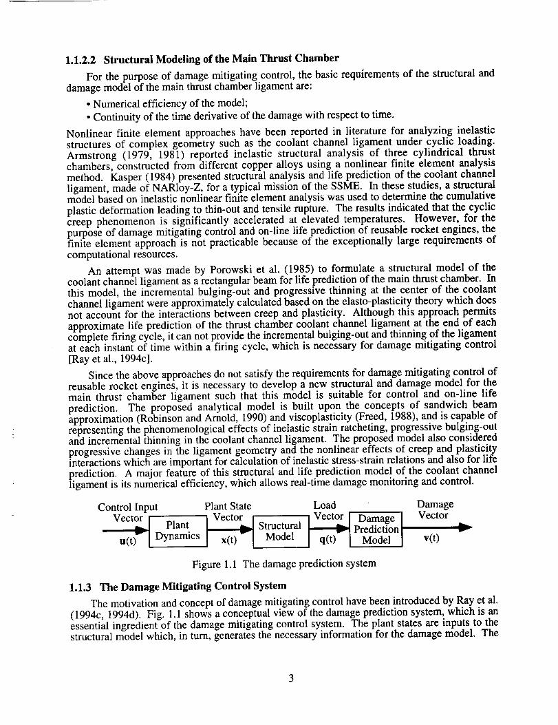
For the purpose of damage mitigating control, the basic requirements of the structural anddamage model of the main thrust chamber ligament are:
• Numerical efficiency of the model;
• Continuity of the time derivative of the damage with respect to time.
Nonlinear finite element approaches have been reported in literature for analyzing inelasticstructures of complex geometry such as the coolant channel ligament under cyclic loading.Armstrong (1979, 1981) reported inelastic structural analysis of three cylindrical thrustchambers, constructed from different copper alloys using a nonlinear finite element analysismethod. Kasper (1984) presented structural analysis and life prediction of the coolant channelligament, made of NARloy-Z, for a typical mission of the SSME. In these studies, a structuralmodel based on inelastic nonlinear finite element analysis was used to determine the cumulativeplastic deformation leading to thin-out and tensile rupture. The results indicated that the cycliccreep phenomenon is significantly accelerated at elevated temperatures. However, for thepurpose of damage mitigating control and on-line life prediction of reusable rocket engines, thefinite element approach is not practicable because of the exceptionally large requirements ofcomputational resources.
An attempt was made by Porowski et al. (1985) to formulate a structural model of thecoolant channel ligament as a rectangular beam for life prediction of the main thrust chamber. Inthis model, the incremental bulging-out and progressive thinning at the center of the coolantchannel ligament were approximately calculated based on the elasto-plasticity theory which doesnot account for the interactions between creep and plasticity. Although this approach permitsapproximate life prediction of the thrust chamber coolant channel ligament at the end of eachcomplete firing cycle, it can not provide the incremental bulging-out and thinning of the ligamentat each instant of time within a firing cycle, which is necessary for damage mitigating control[Ray et al., 1994c].
Since the above approaches do not satisfy the requirements for damage mitigating control ofreusable rocket engines, it is necessary to develop a new structural and damage model for themain thrust chamber ligament such that this model is suitable for control and on-line lifeprediction. The proposed analytical model is built upon the concepts of sandwich beamapproximation (Robinson and Arnold, 1990) and viscoplasticity (Freed, 1988), and is capable ofrepresenting the phenomenological effects of inelastic strain ratcheting, progressive bulging-outand incremental thinning in the coolant channel ligament. The proposed model also consideredprogressive changes in the ligament geometry and the nonlinear effects of creep and plasticityinteractions which are important for calculation of inelastic stress-strain relations and also for lifeprediction. A major feature of this structural and life prediction model of the coolant channelligament is its numerical efficiency, which allows real-time damage monitoring and control.
Control Input Plant State
Vector I I Vector
•..- Plant ,,._
u(t) Dynamics x(t) ""
Load
Structural _
Model ] q(t)
Damage [Prediction [
Model[
DamageVector
v(t)
Figure 1.1 The damage prediction system
1.1.3 The Damage Mitigating Control System
The motivation and concept of damage mitigating control have been introduced by Ray et al.(1994c, 1994d). Fig. 1.1 shows a conceptual view of the damage prediction system, which is anessential ingredient of the damage mitigating control system. The plant states are inputs to thestructural model which, in turn, generates the necessary information for the damage model. The
3
damagemodel is constructedin continuous-time such that the process and damage dynamics canbe simultaneously incorporated within the framework of the control system in the state-variablesetting. A major objective is to quantitatively evaluate the effects of damage rate and damageaccumulation on structural durability under time-dependent thermo-mechanical loading. The
damage state vector v(t) indicates, for example, the level of creep and fatigue damage
accumulation at one or more critical points, and its time derivative i'(t) indicates how the
instantaneous load is affecting the structural components (Ray and Wu, 1994b).
1.2 Objectives and Synopsis of the Report
The discussions above evince the need for interdisciplinary research in the fields of thermo-fluid dynamics, structural dynamics, thermo-mechanical fatigue and creep, and robust control
and decision for enhancement of structural durability and performance of rocket propulsionsystems (Ray et al., 1994d). Fig. 1.2 shows a schematic representation of a damage mitigatingcontrol system which is constructed by integrating the above four interacting disciplines toachieve optimized trade-off between the system performance and structural durability of areusable rocket engine. The procedure for synthesizing a damage mitigating control system forrocket engines is partitioned into the following four tasks:
Task 1: Modeling of the process dynamics of the rocket engine for control system synthesis anddamage evaluation;
Task 2: Modeling of the structural dynamics and damage dynamics of the critical componentssuch as blades of the fuel and oxidizer turbines and the coolant channel ligament in themain thrust chamber;
Task 3: Analysis and synthesis of a feedforward control policy for open loop control of up-thrust transients of the rocket engine;
Task 4: Analysis and synthesis of a feedback control to track the desired open loop trajectory.
The model formulation in Task 1 and Task 2 involves thermal-fluid-structure-materialssystems interactions and must satisfy the following two criteria:
• The model must be sufficiently accurate for damage prediction, plant performanceanalysis, and control systems synthesis;
• The governing equations must be mathematically and computationally tractable togenerate feasible solutions for integrated systems optimization.
In essence, the model must be accurate and numerically efficient for systems analysis and controlsynthesis and, at the same time, provide the necessary information for life prediction and plantperformance evaluation. Task 3 optimizes the plant dynamic performance while maintaining thedamage of critical components of the rocket engine within the prescribed limits. Task 4
compensates for external disturbances and uncertainties in modeling of plant dynamics anddamage dynamics.
The research work in this report focuses on the first three tasks in which a damagemitigating control methodology has been formulated for structural durability and performanceenhancement of reusable rocket engines such as the SSME. A unique feature of the proposeddamage mitigating control is that a substantial gain in service life and maintenance cost can beachieved with no significant reduction in engine performance. The trade-off between service life
and performance is obtained by integrating the plant model with the damage model whichprovides the fatigue/creep damage information for control analysis and synthesis.
A finite-dimensional state-space model of the thermo-fluid propulsion dynamics has beenformulated based on the fundamental principles of fluid flow and thermodynamics. The criticalplant components that are prone to failure include the fuel and oxidizer turbine blades, and the
main thrust chamber coolant wall. Inputs to the structural models are time-dependent plant
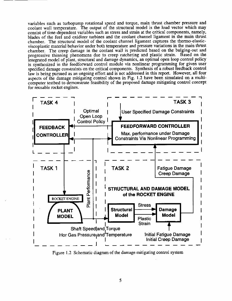
variables such as turbopump rotational speed and torque, main thrust chamber pressure andcoolant wall temperature. The output of the structural model is the load vector which mayconsist of time-dependent variables such as stress and strain at the critical components, namely,blades of the fuel and oxidizer turbines and the coolant channel ligament in the main thrustchamber. The structural model of the coolant channel ligament captures the thermo-elastic-
viscoplastic material behavior under both temperature and pressure variations in the main thrustchamber. The creep damage in the coolant wall is predicted based on the bulging-out andprogressive thinning phenomena due to creep ratcheting and plastic strain. Based on theintegrated model of plant, structural and damage dynamics, an optimal open loop control policyis synthesized in the feedforward control module via nonlinear programming for given userspecified damage constraints on the critical components. Synthesis of a robust feedback controllaw is being pursued as an ongoing effort and is not addressed in this report. However, all fouraspects of the damage mitigating control shown in Fig. 1.2 have been simulated on a multi-computer testbed to demonstrate feasibility of the proposed damage mitigating control conceptfor reusable rocket engines.
[ ! I
TASK 4 I III I Optimal I
Open Loop
1_[, Control Policy 11
L!L I I
TASK 3
User Specified Damage Constraints
FEEDFORWARD CONTROLLER
Max. performance under DamageConstraints Via Nonlinear Programming
n iTASK 1 e I I TASK 2 Fatigue Damage
=o I Creep Damage
•t:: , STRUCTURAL AND DAMAGE MODEL
_ _ ,I [ of the ROCKET ENGINEI ROCKET ENGINE I ,-- I I I
' I_-- StrainShaft SpeedlandlTorque
Hor Gas Pressureland'Temperature Initial Fatigue DamageI Initial Creep Damage
1 .__
Figure 1.2 Schematic diagram of the damage mitigating control system
5
1.3 Contributions of the Reported Research Work
This report presents a unified methodology for damage mitigating control systems analysisand synthesis where the objective is to achieve optimized trade-off between the systemperformance and structural durability of reusable rocket engines such as the SSME. Theproposed methodology integrates the disciplines of thermo-fluid dynamics, mechanicalstructures, and mechanics of materials along with control and optimization of dynamic systems.
The major contribution of this report is the formulation of a new structural and damagemodel of coolant channel ligaments of the main thrust chamber for both on-line life predqctionand damage mitigating control of reusable rocket engines. The structural and damage model isdeveloped based on the theories of sandwich beam and viscoplasticity. This structural model hasproven to be numerically much more efficient than other finite element analysis models, and is ofcomparable accuracy. To the best of the authors' knowledge, no other structural and damagemodel of the main thrust chamber wall is suitable for both control systems synthesis and on-line
life prediction of rocket engines.
Besides rocket engines, the proposed methodology of damage mitigation and life predictionis directly applicable to any thermo-mechanical process such as stream-electric power plants,land-based gas turbines, and aircraft engines where structural durability is a critical issue.
1.4 Organization of the Report
This report is organized into six main chapters including the introduction. Chapter 2presents a simplified nonlinear model of the thermal-fluid dynamics of a rocket engine, similar tothe SSME, which is the plant under control. The results of steady state solutions and transient
responses are discussed. The first part of Chapter 3 presents a brief review of the structuralmodel and the continuous-time fatigue damage model of the turbine blades, which are based onlinear finite element analysis and nonlinear strain-life approach. In the second part of Chapter 3,a new structural and damage model of the coolant channel ligament is developed based on thetheories of sandwich beam and viscoplasticity. By comparison with the nonlinear finite elementanalysis reported by other investigators, Chapter 4 validates the proposed structural and damagemodel of the coolant channel ligament for two different materials, namely, oxygen-free high-
conductivity (OFHC) copper and a copper-zirconium-silver alloy called NARloy-Z. A series ofparametric studies have been conducted corresponding to different design factors of the mainthrust chamber coolant wall, such as ligament materials and configurations, thermo andmechanical loading, and loading cycle duration of the rocket engine. Chapter 5 discusses theprocedure of the damage mitigating control synthesis, and formulates an optimal policy forfeedforward control of up-thrust transients of rocket engines. Results of simulation experimentsand parametric studies are presented for different damage constraints and different initial damageof the critical components. Chapter 6 summarizes and concludes the report along with thedirection for future research and potential technology transfer.
6
CHAPTER 2
THERMO-FLUID DYNAMIC MODELING OF THE REUSABLE ROCKET ENGINE
This chapter presents a nonlinear dynamic model of the thermal-fluid dynamics in a reusablerocket engine. The purpose of this model is to represent the overall dynamic performance andcomponent interactions with sufficient accuracy for control synthesis and damage prediction.The governing equations used in the model are based on the fundamental principles of physics aswell as on the experimental data under a variety of plant operating conditions. The model is
formulated in the state-variable setting via nonlinear differential equations with time-invariantcoefficients.
The operating principles of the rocket engine under consideration are briefly described inSection 2.1. Section 2.2 presents the development of the nonlinear dynamic model equationsusing lumped parameter approximation. Section 2.3 discusses the results of simulationexperiments for model evaluation where the transient responses of the plant state variables due toindependent step disturbances in the control inputs are presented.
2.1 Description of the Reusable Rocket Engine
The reusable bipropellant rocket engine, under consideration in this report, is similar to theSpace Shuttle Main Engine (SSME). Fig. 2.1 shows a functional diagram for operations andcontrol of the rocket engine. The propellants, namely, liquid hydrogen and liquid oxygen, areindividually pressurized by separate turbopumps. Pressurized liquid hydrogen and oxygen arepumped into individual high-pressure preburners which feed the respective turbines with fuel-rich hot gas. The exhaust gas from each turbine is mixed in the common manifold and theninjected into the main combustion chamber where it burns with the oxidizer to make mostefficient use of the energy liberated by combustion. The oxygen flow into each of the twopreburners is independently controlled by the respective servo-valve while the valve position foroxygen flow into the main thrust chamber is held in a fixed position to derive maximum possible
power from the engine. The plant outputs of interest are 0 2 / H 2 mixture ratio and combustor
pressure which are closely related to the rocket engine performance in terms of thrust-to-weightratio and engine efficiency. The liquid hydrogen is used as a regenerative coolant for the wallsof the combustion chamber and thrust nozzle where structural integrity is endangered by the hightemperature environment. The pressurized liquid fuel is circulated through the coolant jackets toabsorb the heat transferred from the hot reaction gases to the thrust chamber and nozzle walls.
2.2 Development of Plant Model Equations
Standard lumped parameter approaches have been used to model the thermo-fluid dynamicsof the engine in order to approximate the partial differential equations describing mass,momentum, and energy conservation by a set of first-order differential equations with time as the
independent variable. The plant model is constructed via causal interconnection of the primarysubsystem models such as the main thrust chamber, preburners, turbopumps, valves, fuel andoxidizer supply headers, and regenerative cooling systems. Fig. 2.2 shows a model solutiondiagram (Ray, 1976 and Ray and Bowman, 1978) of the engine corresponding to the functionaldiagram in Fig. 2.1. Each block in Fig. 2.2 represents a physical plant component or subsystem.The governing equations for the lumped parameter model of the plant dynamics are described inthe following sections. In addition to the basic assumption of the lumped parameter approach,other pertinent assumptions are stated while describing the models of the individual subsystems.
2.2.1 Fuel and Oxidizer Turbopump Subsystems
The rocket engine has two sets of turbopumps, namely, low pressure and high pressure, foreach of the two propellants. A simplified representation of the dynamic characteristics of the
7
rocket engine is developed by lumping the low pressure and high pressure turbopumps into asingle subsystem for each of the fuel and oxidizer propellants as shown in Fig. 2.1. On theoxidizer side, however, two pumps are modeled to obtain two sources of oxygen at different
pressures. Model equations for the fuel and oxidizer turbopumps are given in Table 2.1 andTable 2.2, respectively.
Models of the hydraulic pump subsystems are derived based on the following assumptions:
(a) The pump head which is proportional to the difference between static pressures at thesuction and discharge is derived based on the assumptions of: (i) one-dimensional steady
incompressible flow with negligible heat transfer; (ii) identical fluid velocities at the suction anddischarge section of the pump; and (iii) no change in potential energy
(b) The static performance of the pump is based on empirical characteristics (Rockwell,
1989) where the pump head APpM P, power VpM P, and efficiency l_pMp are modeled as
functions of the ratio of mass flow rate, WpM P, to pump speed S:
AppM P _ S 2 O1(O); VpM P _ S 2 02(0); and TIpMp _ $O3(O) (2.1)
where O = WpM P ] S, and the functions • 1, 0 2, and • 3 are obtained from Rockwell (1989).
Therefore, the outputs of the pump model, namely, pump discharge pressure, temperature,enthalpy, and torque, can be obtained from the pump characteristics and thermodynamic staterelations.
The governing equations for the turbine model are formulated under the following
assumptions:
(c) The working fluid in the turbine is a perfect gas and the expansion process in the turbineis adiabatic. For the ideal frictionless process, the following relationship holds:
Tin / Tout,ideal = (Pin / Pout)(k-l)/k (2.2)
where T is the absolute temperature, P is the pressure, the subscripts "in" and "out" respectivelyindicate the inlet and the outlet of the turbine, the subscript "ideal" stands for the idealized
isentropic condition, and k is the ratio of the specific heats at constant pressure and temperature,which is assumed to be a constant within the operating range of turbine.
(d) No loss of pressure and enthalpy occurs between the preburner outlet and turbine inlet.That is,
PPBR = PTRB,in; and HpB R = HTRB,in (2.3)
(e) Flow through the turbine is assumed to be choked, and the kinetic energy of the fluid in
the preburner chamber is negligible such that the stagnation pressure and temperature, P* and
T*, are respectively identical to the static preburner pressure and temperature, P and T.Therefore, the mass flow rate WTRB through the turbine can be expressed as:
P'_RB,in PPBR C PPBR (2.4)
WTR B = C _TTRB,in, = C _ = _T_PBR
where the coefficient C is calculated from the steady-state data.
(f) The turbine efficiency and the output torque are obtained from the empiricalcharacteristics of the turbine (Rockwell, 1989) as:
, SrITRS= rlTRBO(_)
S
XTR B = WTRB_AI--Iideal tl)(_)
where ideal(i.e.,isentropic)enthalpydrop AHideaIisgiven as:
ToutEIPo eal l pTinI I pTin'
(2.5a)
(2.5b)
(2.6)
The outputs of the fuel and oxidizer turbine models, namely, turbine pressure, temperature,enthalpy, flow rate, and output torque are obtained from thermodynamic relations as delineatedin Tables 2.1 and 2.2, respectively.
The state variables in the fuel and oxidizer turbopump subsystems are respectively the shaft
speeds SpM P and SoPMP. The power delivered by each turbine is equal to the sum of the power
required by the propellant pump, and power losses in the bearings, gears, seals, and wear rings.Therefore, the dynamics of shaft speed in each turbopump are given m terms of the difference m
torque as:
IdS = (XTR s _ XpMp ) (2.7)dt
where I is the moment of inertia and X indicates the torque.
2.2.2 Preburner Fuel and Oxidizer Supply Header Subsystems
The model equations of the prebumer fuel and oxidizer supply header subsystems are listedin Table 2.3. The equations of fuel flow to each prebumer are approximated to simplify the
complexity of flow boundaries. The fuel flow to the two prebumers accounts for the mixture ofthe coolant flow from the primary nozzle cooling region and the primary nozzle bypass. Thegoverning equations of the fuel flow through the preburner header are derived under thefollowing assumptions:
(a) The prebumer fuel supply pressure P_s is proportional to the fuel flow pressure at the
main fuel valve.
(b) Two coolant flows, namely, main chamber coolant flow (WCMBF) and primary nozzle
coolant flow (WNozF), varies in proportion to the total fuel flow (WpMp). Since the coolant
control valve position is held fixed, it is treated as fully open. Accordingly, the fixed nozzle
bypass flow WFrCa P is obtained by subtracting the main chamber coolant flow and the nozzlecoolant flow as:
WCMBF = CCMBFWpMp
WNOZF = CNozFWpM P
WFNBP = WpM P -- WCMBF -- WNOZF
(2.8a)
(2.8b)
(2.8c)
By neglecting the dynamics due to fluid inertance in the flow passages, the above simplifications(a) and (b) reduce four differential equations of momentum conservation into four algebraic
f L p Q2 CIWlWae= p ,
equations. This approximation only affects the model accuracy at high frequencies because ofrelatively small fluid inertance.
(c) For one dimensional, incompressible uniform flow through a pipeline or valve and
neglecting the body force, the friction pressure drop through a pipeline or valve is expressed as:
C = f___L 1 for pipeline (2.9a)D 2A 2 '
AP=f LpQ2--C 'lwlw c' =fL 1 AD 2 A 2 RA 2 ' D 2pA 2' RA = __ for valve (2.9b)
A
The state variables of the preburner fuel and oxidizer supply headers are:
W_IPB H and WHPBO (fuel mass flow rates into the fuel and oxidizer preburners);
WOPBH and WOPBO (oxidizer mass flow rates into the fuel and oxidizer preburners).
The derivatives
momentum over a control volume of a pipeline,
_'t (w) = Cf(Pin - Pout -),Iwlw
CP
where p is the average fluid density and Cf is the inverse of equivalent fluid inertance.
of the above four state variables are obtained from conservation of linear
(2.10)
2.2.3 Main Chamber Fuel Injector Subsystem
The fuel injector mixes the two branches of fuel-rich exhaust hot-gas from the two turbinesand a small amount of fuel from the combustion chamber coolant path. Model equations for the
preburners, main thrust chamber, and fuel injector are listed in Table 2.4. The governing
equations of the fuel injector subsystem are derived under the following assumptions:
(a) The flow of an incompressible working fluid at a low Mach number (e.g., M< 0.3) is
governed by the following relation (Blackburn et al., 1960) by assuming that the subsonicvelocities exist throughout the orifices:
Q = 'oA = C'dA_/2(Pin - Pout ) /
W = Qp = C d _/2(Pin - Pout)P
(volumetric flow rate) (2.12a)
(mass flow rate) (2.12b)
where _ is the average density which is approximated as the gas density PCMB at the combustor.
(b) The flow into the fuel injector manifold is the sum of two turbine exhaust flows, WTRB
and WOT R, and main combustion chamber coolant flow WCMBF. The manifold pressure PFINJ
is derived form Eq. (2.12b) as:
PFINJ (WTRB +WoTR + WCMBF)2 +PcMB (2.13)= C2 PCMB
(c) The mixed gas temperature at the fuel injector manifold is obtained as a weighted
average of the two turbine inlet temperatures, TpB R and Top B, and the main chamber coolant
flow temperature, TCMBF. That is, TFINJ =CoTpBR+C1ToPB+C2TcMBF where the
coefficients, C d , C 0, C !, and C 2 are obtained from the steady-state data under normal operating
conditions.
10

2.2.4 Oxygen Control Valve Subsystem
The nonlinearities of control valves are compensated by inducing the inverse characteristics
of valves (Rockwell, 1989) in the control signal such the valve command becomes proportionalto the valve area under steady-state operations. The oxygen control valve subsystem model has
two state variables, namely, fuel and oxidizer preburner valve rotary positions. The dynamics ofeach valve are represented by a first order lag as:
d(AR_v) = AR_V - U_v (2.15a)XFPV
d (ARoPV) (2.15b)AROPV UoPv
'lTopv
where UFp v and Uop V are the commands to the oxygen control valves, and ARFPV and AROPV
are the effective areas of the oxidizer control valves, and 'r is the time constant of the respectivevalve.
In solving the nonlinear optimal open loop control problem, the two commands U_v and
Uov v correspond to the decision variables in the nonlinear programming which are bounded
above and below via specified constraints.
2.2.5 Preburner and Combustion Subsystems
The dynamic equations for the combustion process are developed by employing theprinciples of conservation of mass and energy with following assumptions.
(a) Conservation of momentum is satisfied by assuming that gas pressure and temperaturein the combustion chamber are spatially uniform although they are time-dependent, and thekinetic energy due to gas velocity in the chamber is negligible. This assumption is valid for alow-frequency dynamic representation, and precludes the process of high-frequency acousticpropagation.
(b) One-dimensional unsteady flow in the combustion chamber is represented by a firstorder differential equation of the rate change of mixture gas density which is related to the massflow into and out of the chamber via conservation of mass.
_tt(P) = Win-- Wou t (2.16)VCMB
where VCM B is the volume of the combustion chamber.
(c) The conservation of energy equation yields:
d(CvVpT) = _WinHin - _WoutHout + FWo 2 - Qheat (2.17)
where F is the energy liberated by per unit mass of oxygen from a macroscopic point of view of
the chemical process where the reaction dynamics is assumed to be instantaneous. Qheat is theheat transfer rate from the control volume to the coolant channel wall.
(d) Based on the thermodynamic relationship of the perfect gas law, the average gas
temperature in the combustion chamber is given as: TCM B = PCMB /(PCMB R) where R is the
characteristic gas constant. Therefore, the derivative of the main chamber pressure is obtainedby rewriting the energy Eq. (2.17) as:
11
d_'(PcMa) = (WFINjHFINJ + WCMBOHoP2E - WNozHcMB (2.18)
+ WCMaoF - QcMBw) / (CvVcMB / R)
(e) The flow through the nozzle throat is choked.
The model equations of the preburner and combustor are given in Table 2.4. The six statevariables in two preburners and main combustion chamber are:
• PPBR and RpB R: (Fuel prebumer chamber gas pressure and density);
• PoPB and Rot, B: (Oxidizer prebumer chamber gas pressure and density);
• PCMa and RCMa: (Main thrust chamber hot gas pressure and density).
The governing equations in preburners are similar to those in the main chamber because ofthe similarity of the physical processes.
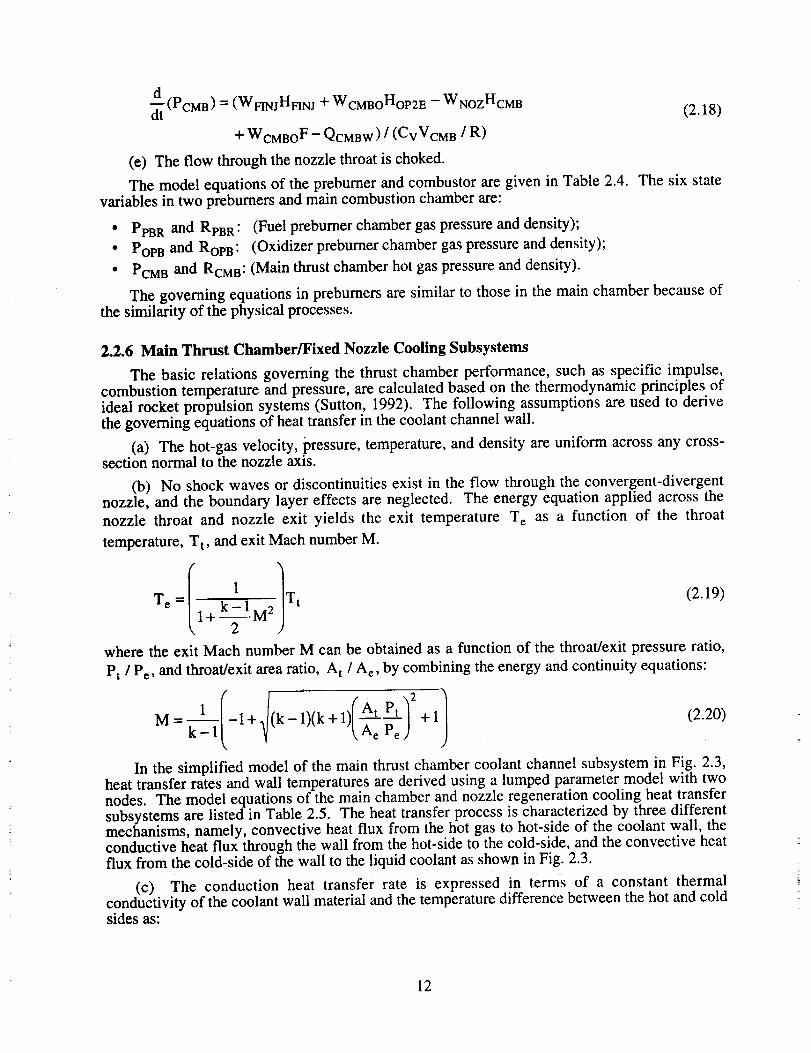
2.2.6 Main Thrust Chamber/Fixed Nozzle Cooling Subsystems
The basic relations governing the thrust chamber performance, such as specific impulse,
combustion temperature and pressure, are calculated based on the thermodynamic principles ofideal rocket propulsion systems (Sutton, 1992). The following assumptions are used to derivethe governing equations of heat transfer in the coolant channel wall.
(a) The hot-gas velocity, pressure, temperature, and density are uniform across any cross-section normal to the nozzle axis.
(b) No shock waves or discontinuities exist in the flow through the convergent-divergentnozzle, and the boundary layer effects are neglected. The energy equation applied across the
nozzle throat and nozzle exit yields the exit temperature T e as a function of the throat
temperature, T t, and exit Mach number M.
1
Te = " k - 1 M2 Tt (2.19)1+ 2
where the exit Mach number M can be obtained as a function of the throat/exit pressure ratio,
Pt / Pe, and throat/exit area ratio, A t / A e, by combining the energy and continuity equations:
M = -1 + (k- 1)(k + 1) _ee + 1 (2.20)
In the simplified model of the main thrust chamber coolant channel subsystem in Fig. 2.3,heat transfer rates and wall temperatures are derived using a lumped parameter model with twonodes. The model equations of the main chamber and nozzle regeneration cooling heat transfersubsystems are listed in Table 2.5. The heat transfer process is characterized by three differentmechanisms, namely, convective heat flux from the hot gas to hot-side of the coolant wall, theconductive heat flux through the wall from the hot-side to the cold-side, and the convective heatflux from the cold-side of the wall to the liquid coolant as shown in Fig. 2.3.
(c) The conduction heat transfer rate is expressed in terms of a constant thermalconductivity of the coolant wall material and the temperature difference between the hot and coldsides as:
12
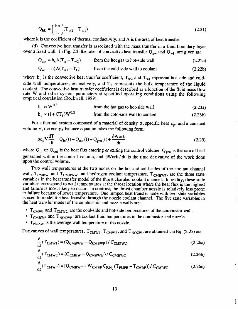
Qhk = (-_](Tw2 - Twl) (2.21)
where k is the coefficient of thermal conductivity, and A is the area of heat transfer.
(d) Convective heat transfer is associated with the mass transfer in a fluid boundary layer
over a fixed wall. In Fig. 2.3, the rates of convective heat transfer Qgw and Qwf are given as:
Qgw = hcA(Tg - Tw2) from the hot gas to hot-side wall (2.22a)
Qwf = hcA(Twl - Tf) from the cold-side wall to coolant (2.22b)
where h c is the convective heat transfer coefficient, Tw2 and Twl represent hot-side and cold-
side wall temperatures, respectively, and Tf represents the bulk temperature of the liquidcoolant. The convective heat transfer coefficient is described as a function of the fluid mass flow
rate W and other system parameters at specified operating conditions using the followingempirical correlation (Rockwell, 1989):
h e ,,_ W °'8 from the hot gas to hot-side wall (2.23a)
h c o_ (1 + CTf)W 0"8 from the cold-side wall to coolant (2.23b)
For a thermal system composed of a material of density P, specific heat Cp, and a constant
volume V, the energy balance equation takes the following form:
dT _iWork (2.25)pcpV-_- = Qin (t) - Qout (t) + Qgen(t) + dt
where Qin or Qout is the heat flux entering or exiting the control volume, Qgen is the rate of heat
generated within the control volume, and _SWork/dt is the time derivative of the work doneupon the control volume.
Two wall temperatures at the two nodes on the hot and cold sides of the coolant channel
wall, TCMBW and TCMBWW, and hydrogen coolant temperature, TCMBWF, are the three state
variables in the heat transfer model of the thrust chamber coolant channel. In reality, these statevariables correspond to wall temperatures at the throat location where the heat flux is the highestand failure is most likely to occur. In contrast, the thrust chamber nozzle is relatively less proneto failure because of lower temperature. One lumped heat transfer node with two state variablesis used to model the heat transfer through the nozzle coolant channel. The five state variables inthe heat transfer model of the combustion and nozzle walls are:
° TCMWI and TCMW2 are the cold-side and hot-side temperatures of the combustor wall.
° TCMBWF and TNOZWF: are coolant fluid temperatures in the combustor and nozzle.
° TNOZW is the average wall temperature of the nozzle.
Derivatives of wall temperatures, TCMWl, TCMW2, and TNOZW, are obtained via Eq. (2.25) as:
d_t (TcMw1) = (QcMnww - QCMBWF) CCMBWC/
d_t (TcMw2) = (QcMBW -- QCMBWW) CCMBWC/
d
_-(TcMwF) = [QcMBWF + WCMBF Cp,H 2 (TpMPE -- TCMBF)] / CCMBFC
(2.26a)
(2.26b)
(2.26c)
13
Thecold-sideandhot-sidetemperatures,TCMWI and TCMW2, of the combustor wall are denoted
as T 1 and T2 for brevity in the creep damage model in Chapter 3.
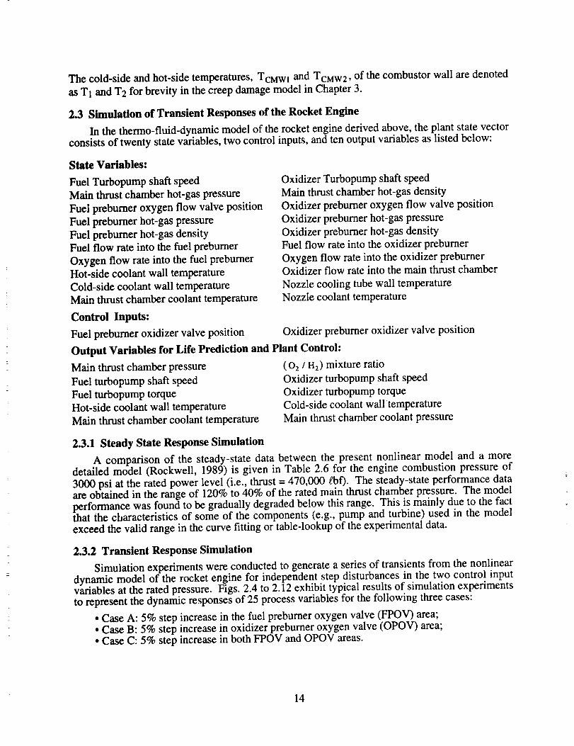
2.3 Simulation of Transient Responses of the Rocket Engine
In the thermo-fluid-dynamic model of the rocket engine derived above, the plant state vectorconsists of twenty state variables, two control inputs, and ten output variables as listed below:
State Variables:
Fuel Turbopump shaft speed
Main thrust chamber hot-gas pressure
Fuel preburner oxygen flow valve position
Fuel prebumer hot-gas pressure
Fuel prebumer hot-gas density
Fuel flow rate into the fuel preburner
Oxygen flow rate into the fuel preburner
Hot-side coolant wail temperature
Cold-side coolant wail temperature
Main thrust chamber coolant temperature
Control Inputs:
Fuel prebumer oxidizer valve position
Oxidizer Turbopump shaft speed
Main thrust chamber hot-gas density
Oxidizer prebumer oxygen flow valve position
Oxidizer prebumer hot-gas pressure
Oxidizer prebumer hot-gas density
Fuel flow rate into the oxidizer preburner
Oxygen flow rate into the oxidizer preburner
Oxidizer flow rate into the main thrust chamber
Nozzle cooling tube wail temperature
Nozzle coolant temperature
Oxidizer preburner oxidizer valve position
Output Variables for Life Prediction and Plant Control:
Main thrust chamber pressure
Fuel turbopump shaft speed
Fuel turbopump torque
Hot-side coolant wail temperature
Main thrust chamber coolant temperature
( 02 / H2) mixture ratio
Oxidizer turbopump shaft speed
Oxidizer turbopump torque
Cold-side coolant wall temperature
Main thrust chamber coolant pressure
2.3.1 Steady State Response Simulation
A comparison of the steady-state data between the present nonlinear model and a moredetailed model (Rockwell, 1989) is given in Table 2.6 for the engine combustion pressure of
3000 psi at the rated power level (i.e., thrust = 470,000 fbf). The steady-state performance dataare obtained in the range of 120% to 40% of the rated main thrust chamber pressure. The modelperformance was found to be gradually degraded below this range. This is mainly due to the factthat the characteristics of some of the components (e.g., pump and turbine) used in the modelexceed the valid range in the curve fitting or table-lookup of the experimental data.
2.3.2 Transient Response Simulation
Simulation experiments were conducted to generate a series of transients from the nonlinear
dynamic model of the rocket engine for independent step disturbances in the two control inputvariables at the rated pressure. Figs. 2.4 to 2.12 exhibit typical results of simulation experimentsto represent the dynamic responses of 25 process variables for the following three cases:
• Case A: 5% step increase in the fuel prebumer oxygen valve (FPOV) area;* Case B: 5% step increase in oxidizer prebumer oxygen valve (OPOV) area;* Case C: 5% step increase in both FPOV and OPOV areas.
14
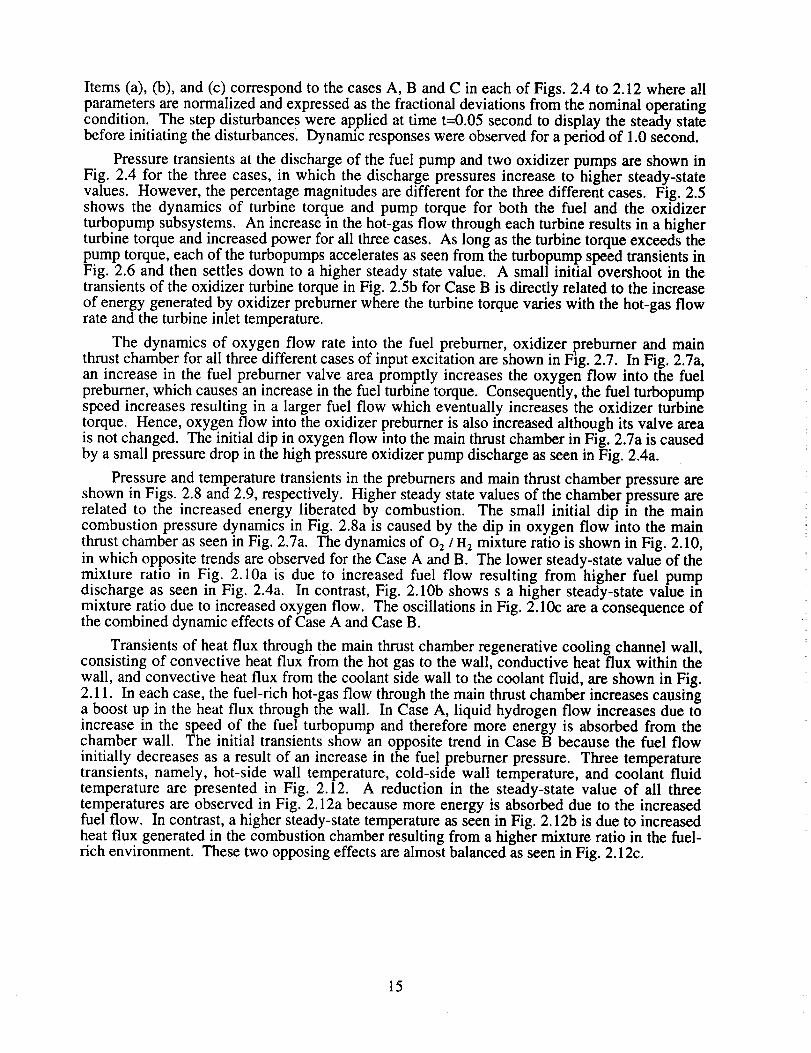
Items (a), (b), and(c) correspondto the casesA, B andC in eachof Figs.2.4 to 2.12whereallparametersarenormalizedandexpressedasthefractionaldeviationsfrom thenominaloperatingcondition. Thestepdisturbanceswereappliedat time t=0.05secondto display thesteadystatebeforeinitiating thedisturbances.Dynamicresponseswereobservedfor aperiodof 1.0second.
Pressuretransientsat thedischargeof the fuel pumpandtwo oxidizer pumpsareshowninFig. 2.4 for the threecases,in which the dischargepressuresincreaseto higher steady-statevalues. However,thepercentagemagnitudesaredifferent for thethreedifferentcases.Fig. 2.5shows the dynamics of turbine torque and pump torque for both the fuel and the oxidizerturbopumpsubsystems.An increasein thehot-gasflow througheachturbineresultsin a higherturbinetorqueandincreasedpowerfor all threecases.As long astheturbinetorqueexceedsthepumptorque,eachof theturbopumpsacceleratesasseenfrom theturbopumpspeedtransientsinFig. 2.6 and thensettlesdown to a higher steadystatevalue. A small initial overshootin thetransientsof theoxidizer turbinetorquein Fig. 2.5bfor CaseB is directly relatedto the increaseof energygeneratedby oxidizerpreburnerwheretheturbinetorquevarieswith the hot-gasflowrateandtheturbineinlet temperature.
The dynamicsof oxygen flow rate into the fuel prebumer,oxidizer preburnerand mainthrustchamberfor all threedifferentcasesof input excitationareshownin Fig. 2.7. In Fig. 2.7a,an increasein the fuel preburnervalve areapromptly increasesthe oxygen flow into the fuelpreburner,whichcausesanincreasein thefuel turbinetorque. Consequently,thefuel turbopumpspeedincreasesresulting in a larger fuel flow which eventuallyincreasestheoxidizer turbinetorque. Hence,oxygenflow into theoxidizerpreburneris alsoincreasedalthoughits valve areais notchanged.Theinitial dip in oxygenflow into themainthrustchamberin Fig. 2.7ais causedby asmallpressuredrop in thehighpressureoxidizerpumpdischargeasseenin Fig. 2.4a.
Pressureandtemperaturetransientsin thepreburnersandmainthrustchamberpressureareshownin Figs. 2.8and2.9,respectively.Highersteadystatevaluesof thechamberpressurearerelated to the increasedenergy liberatedby combustion. The small initial dip in the maincombustionpressuredynamicsin Fig. 2.8ais causedby the dip in oxygenflow into the mainthrustchamberasseenin Fig. 2.7a. Thedynamicsof o2/H2 mixture ratio is shown in Fig. 2.10,in which opposite trends are observed for the Case A and B. The lower steady-state value of themixture ratio in Fig. 2.10a is due to increased fuel flow resulting from higher fuel pumpdischarge as seen in Fig. 2.4a. In contrast, Fig. 2.10b shows s a higher steady-state value inmixture ratio due to increased oxygen flow. The oscillations in Fig. 2.10c are a consequence ofthe combined dynamic effects of Case A and Case B.
Transients of heat flux through the main thrust chamber regenerative cooling channel wall,consisting of convective heat flux from the hot gas to the wall, conductive heat flux within the
wall, and convective heat flux from the coolant side wall to the coolant fluid, are shown in Fig.2.11. In each case, the fuel-rich hot-gas flow through the main thrust chamber increases causinga boost up in the heat flux through the wall. In Case A, liquid hydrogen flow increases due toincrease in the speed of the fuel turbopump and therefore more energy is absorbed from thechamber wall. The initial transients show an opposite trend in Case B because the fuel flowinitially decreases as a result of an increase in the fuel prebumer pressure. Three temperaturetransients, namely, hot-side wall temperature, cold-side wall temperature, and coolant fluidtemperature are presented in Fig. 2.12. A reduction in the steady-state value of all threetemperatures are observed in Fig. 2.12a because more energy is absorbed due to the increased
fuel flow. In contrast, a higher steady-state temperature as seen in Fig. 2.12b is due to increasedheat flux generated in the combustion chamber resulting from a higher mixture ratio in the fuel-
rich environment. These two opposing effects are almost balanced as seen in Fig. 2.12c.
15
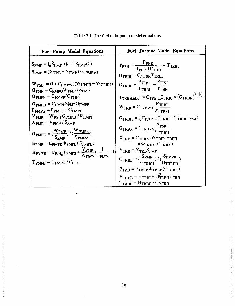
Table 2.1 The fuel turbopump model equations
Fuel Pump Model Equations
SpM P = j'_)SpMp(t)dt + SpMp(0)
SpMP = (XTRB - XpMP) / CpMPMI
WpM P = (I + CpMPw)(WHPBH + WOPBH)
GpM P = CpMPGWpMp / SpMp
GpMPP = _PMPP (GpMP)2
GpMPD = CpMppSpMpGpMpp
PPMPE = PPMPS + GpMPD
VpM P = WpMpGpMPD / RpMPI
XpM P = VpM P / SpMp
GpMPE = (WPMP ) / (.WpMPR.)SpMP SpMPR
EpM P = EpMPR_PMPE(GpMPE)
HpMPE = Cp,H2TpMPS 4 VpM p (__._l_WpMp l"lpMp
TpMPE = HpMPE / Cp,H 2
Fuel Turbine Model Equations
TpBR = PPBR = TTRB IRpBRRCTBu
HTRBI = Cp,PBRTTRBI
PTRBE = PFINJGTRBP =-
PTRBI PPBR
TTRBE,ideal = CTRBTITTRBI × (GTRB P)k-/l/k
PTRBI
WTR B = CTRBW 3
GTRBH = qCp,TRB(TTRBI - TTRBE,ideal)
SpMPGTRBX = CTRBX 5 --
GTRBH
XTR B = CTRBX5WTRBGTRBH
x OTRBX (GTRBX)
VTR B = XTRBSpMp
GTRBE = ( SpMP )/( SpMPR )GTRBH GTRBHR
ETRB = ETRBROTRBE(GTRBE)2
HTRBE = HTRBI - GTRBHETRB
TTRBE = HTRBE / Cp,TRB
16
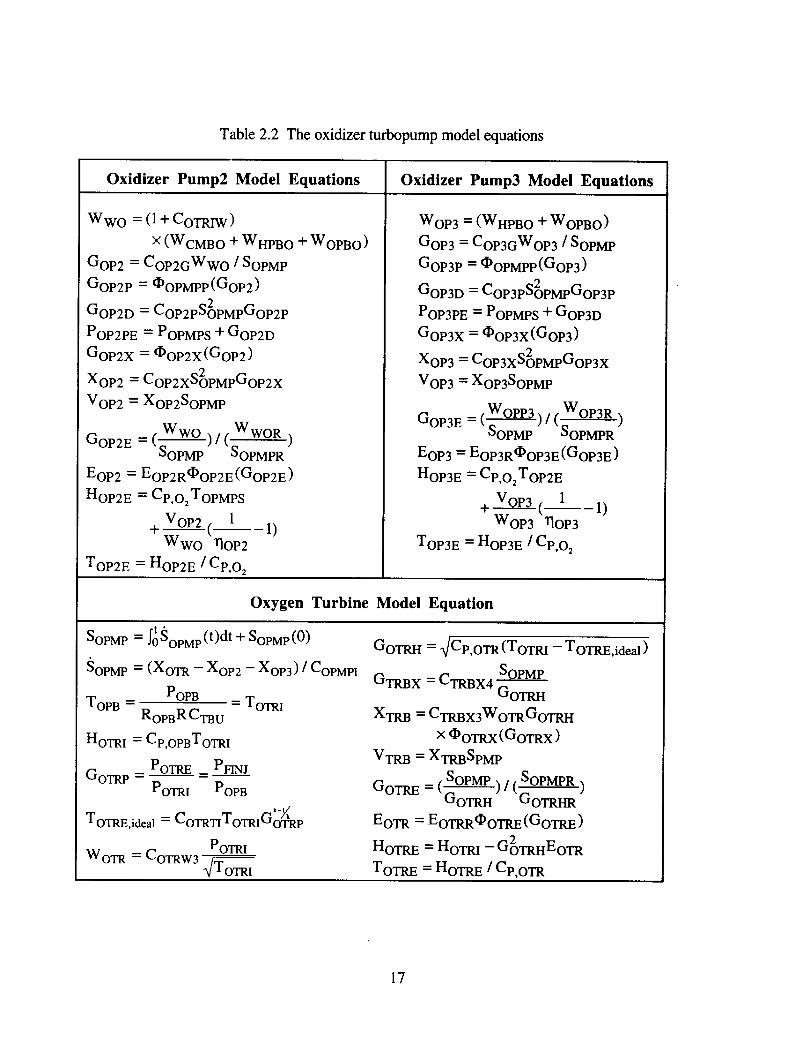
Table 2.2 The oxidizer turbopump model equations
Oxidizer Pump2 Model Equations Oxidizer Pump3 Model Equations
Wwo = (1 + COTRI w)
× (WcMBO + WHPBO + WoPBO)
Gop 2 = COP2GWwo / SoPMP
GOP2P = _OPMPP (GoP2)
2GOP2D = CoP2pSoPMpGoP2P
POP2PE = POPMPS + GOP2D
GOP2X = _OP2x(GoP2)
2Xop 2 = CoP2xSoPMpGoP2x
Vop 2 = XoP2SoPMP
WWO WGoP2 E=( )/(WOR.)
SOPMP 5OPMPR
Eop 2 = EOP2Rt_OP2E (GoP2E)
HOP2E = Cp,02ToPMP S
+ Vop 2 ( 1 1)
Wwo TIOP2
TOP2E = HOP2E /Cp,o 2
Wop 3 = (WHPBO + WoPBO)
Gop 3 = CoP3GWop 3 / SoPMP
GoP3P = _OPMpp(GoP3)
2GOP3D = CoP3pSOPMpGoP3P
POP3PE = POPMPS + GOP3D
GoP3X = OOP3X (GoP3)
2Xop 3 = COP3xSoPMpGoP3X
Vop 3 = XoP3SoPMP
GOP3E = (WoPP3) / ( WOP3R )_OPMP SOPMPR
Eop 3 = EOP3R_OP3E (GoP3E)
HOP3E = Cp,o2ToP2E
+ Vop 3 ( 1 1)WoP3 "TiOP 3
TOP3E = HOP3E / Cp,o 2
Oxygen Turbine Model Equation
SOPMP = _0SOPMP (t)dt + SoPMP (0)
SOPMP = (XoT R - Xop 2 - Xop 3) / CoPMP I
TOPB = POPB = TOTR 1RoPBRCTI3U
HOTRI = Cp,oPBTOTRI
GOTR P = POTRE _ PFINJPOTRI POPB
TOTRE,ideal = ,,..OTRTIIOTRI__,OTRP
POTRI
WOTR = COTRW3 _OTRI
GOTRH = _Cp,oy R (ToTRI - TOTRE,ideal )
GTRBX = CTRBX 4 SOPMPGOTRH
XTR B = CTRBx3WoTRGOTRH
x OOTRX (GoTRX)
VTR B = XTRBSpM P
GOTRE = (SoPMP) / ( SOPMPR )GOTRH GOTRHR
EOT R = EOTRR_OTRE(GOTRE)
HOTRE = HOTRI - G2TRHEOTR
TOTRE = HOTRE / Cp,OT R
17
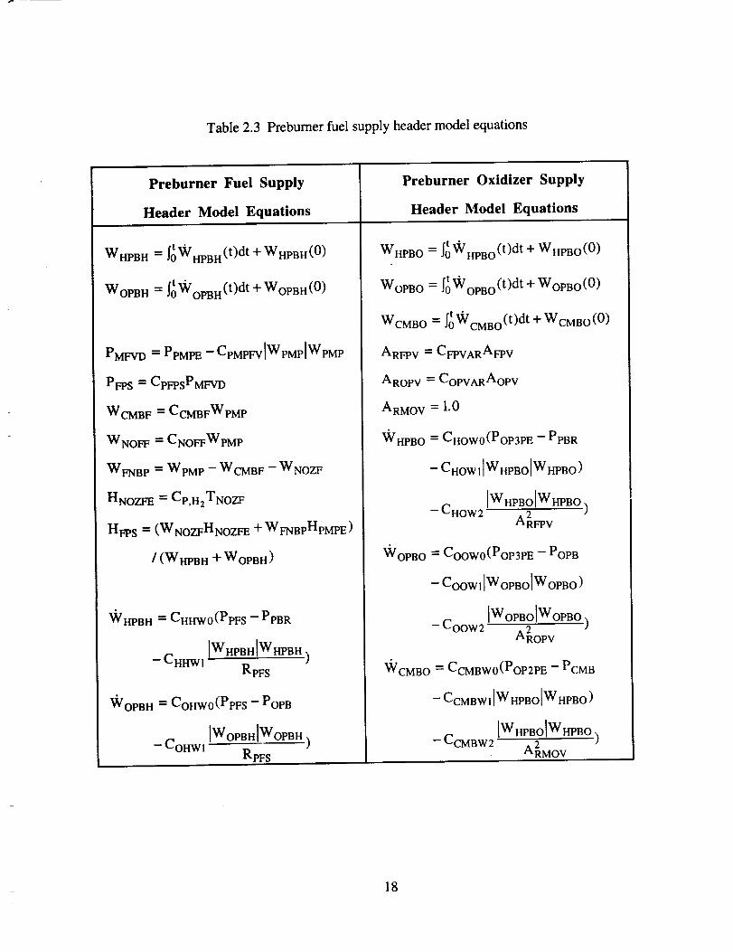
Table 2.3 Prebumer fuel supply header model equations
Preburner Fuel Supply
Header Model Equations
WHPBH= f0WHPBH(t)dt + WHPBH(0)
WOPBH= J_WOPBH(t)dt + WOPBH (0)
PMFVD = PPMPE - CpMPFvIWpMpIWpMP
Preburner Oxidizer Supply
Header Model Equations
WHPBO = _0"VlV'HPBO(t)dt + WHPBO(0)
t "WoPao = _ WOPBO (t)dt + WOPBO (0)
WCMBO = _ WCMBO(t) dt+ WCMBO(O)
ARFPV = CFPVARAFp v
P_s = CpFPsPMFVD
WCMBF = CCMBFWpMp
WNOFF = CNOFFWpM P
WF-NB P = WpM P -- WCMBF -- WNOZF
HNOZF E = Cp,H2TNozF
HFp s = (WNozFHNozF E + WFNBpHpMPE)
AROPV = COPVARAoPv
ARMOV = 1.0
WHPBO = CHOw0(PoP3PE -- PPBR
- CHOW1[WHpBo[WupBo)
WHPBO WHPBO )-- CHOW2 A2 v
/ (WFIPB H -I- WOPBH )
"V_rHPBH = CHHW0(PPFs -- PPBR
- CHHW1 ]WHPBH]WHPBH.)
RpFS
XidOPBH = COHw0(PPFs - POPB
-- COHWl ]WoPBHIWOPBH,)
RpFS
"VVoPBO = Coowo(PoP3PE - POPB
-- COOW1 ]WoPBo]WoPBO)
[WoPBoIWoPBo-- COOW2 2 )
AROPV
WCMBO = CCMBw0(PoP2PE - PCMB
-- CCMBWI[WHPBO[WHPBO)
]WHPBO ]W HPBO )-- CCMBW2 2
ARMOV
18
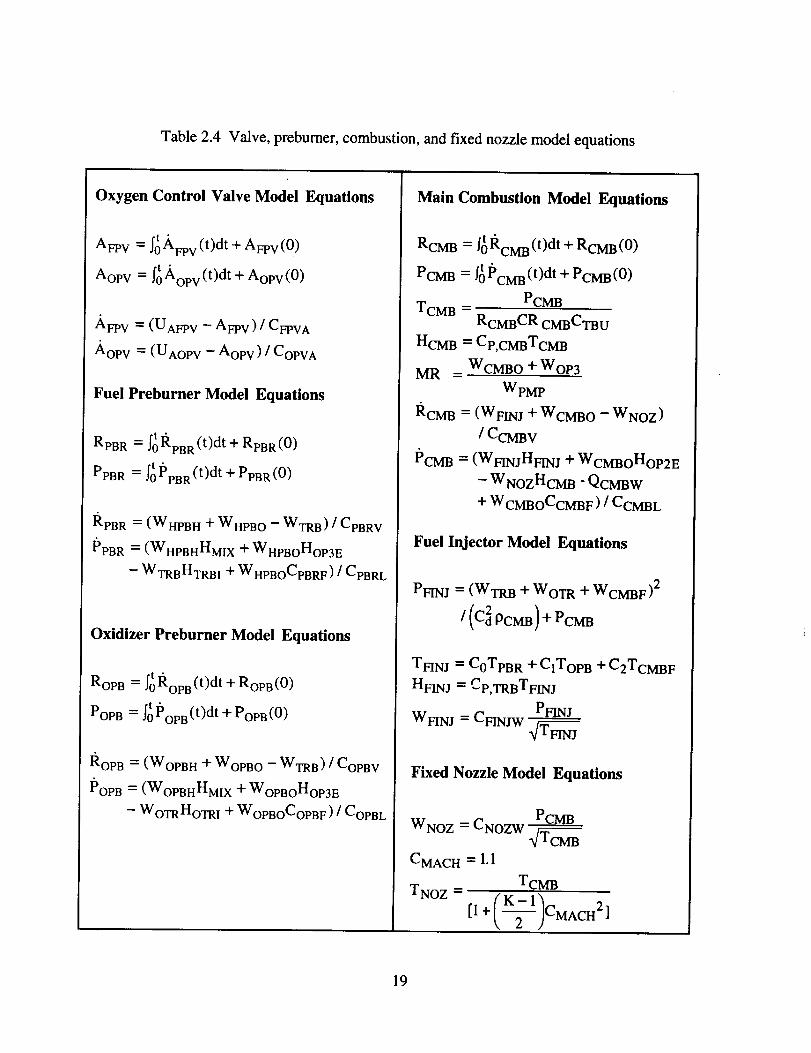
Table2.4 Valve,preburner,combustion,andfixednozzlemodelequations
Oxygen Control Valve Model Equations
t •
AFp v = f_AFp v (t)dt + AFpv(0)
Aop V = f_ Aop v (t)dt + AoPv(0)
AFPV = (UAFPV -- AFPV ) / CFPVA
Aop v = (UgoPv - Aop V) / COPVA
Fuel Preburner Model Equations
RpB R = _ l_pB R (t)dt + RpB R (0)
PPBR = _0PPBR(t) dt + PPBR(0)
RpB R = (WHPBH + WHPBO -- WTRB) [ CpBRV
PPBR = (WHPBHHMIx + WHPBOHOP3E
- WTRBHTRBI + WHPBOCpBRF) / CpBRL
Oxidizer Preburner Model Equations
Rop B = _l_oPB(t)dt + ROPB(0)
POPB = _0POPB (t)dt+ POPB (0)
Rop B = (WoPBH + WoPBO - WTRB) ] COPBV
POPB = (WoPBHHMIx + WOPBOHOP3E
- WoTRHOTRI + WOPBOCOPBF) / COPBL
Main Combustion Model Equations
RCM B = f_l_cMB(t)dt + RCMB(0)
PCMB = f_ PCMB (t)dt + PCMB(0)
TCMB = PCMBRcMBCR cMBCTBu
HCM B = Cp,cMBTCM B
MR = WCMBO + WOP3
WpMP
I_CMB = (WFINJ + WCMB 0 - WNOZ)
/CCMBV
PCMB = (WFINjHFINJ + WCMBOHOP2E
- WNozHcMB "QCMBW
+ WCMBOCCMB F) / CCMB L
Fuel Injector Model Equations
PFINJ = (WTRB + WOTR + WCMBF)2
/ (C2 PCMB) + PCMB
TFINj = CoTpB R + ClTop B + C2TCMBF
HFINj = CP,TRBTFINJ
PFINJ
WFINJ = CFINJ W
Fixed Nozzle Model Equations
PCMB
WNO z = CNOZW
CMACH = 1.1
TNO Z = TCMB
[1 + (-_]CMACH 2 ]
19
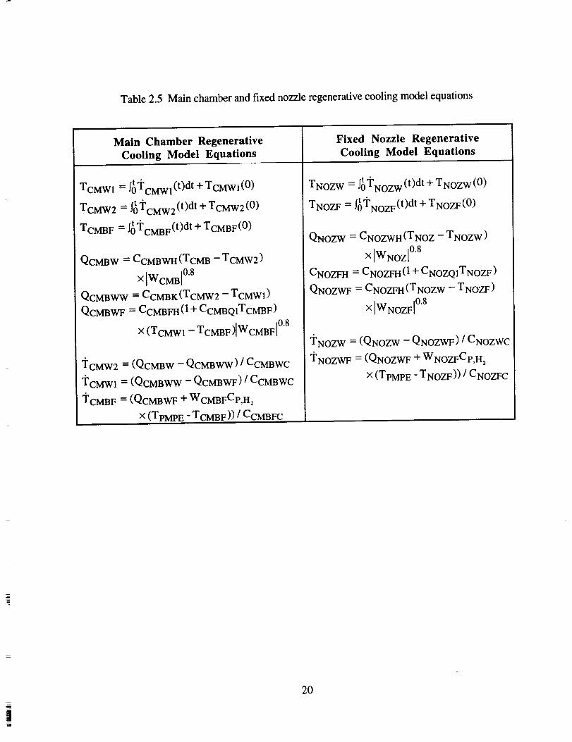
Table 2.5 Main chamber and fixed nozzle regenerative cooling model equations
Main Chamber Regenerative
Cooling Model Equations
t °
TCMW1 = _TcMwl (t)dt + TCMWl (0)
TCMW2 = _i'CMW2 (t)dt + TCMW2 (0)
TCMBF = J_TcMBF(t)dt + TCMBF(0)
QCMBW = CCMBWH(TCMB - TCMW2 )
× WCMB[ 0"8
QCMBWW = CCMBK(TcMw2 - TCMW1)
QCMBWF = CCMBFH (1 + CCMBQITCMBF)
× (TcMw 1 - TCMBF)IWCMBF[ 0"8
"FCMW2 = (QcMBW - QCMBWW) / CCMBWC
"FCMWl = (QcMBWW - QCMBWF) / CCMBWC
"FCMBF = (QcMBWF + WCMBFCp,H:
× (TpMPE - TCMBF )) / CCMBFC
Fixed Nozzle Regenerative
Cooling Model Equations
TNOZW = J_'i_NOZW (t)dt + TNOZW (0)
TNOZF = J0'rNOZF (t)dt + TNOZF (0)
QNOZW = CNOZWH (TNoz - TNOZW)
x IWNoz 0.8
CNOZF H = CNOZF H (1 + CNOZQITNOzF)
QNOZWF = CNOZFH (TNozw - TNOZF)
XIWNozF[ °'8
TNOZW = (QNozw - QNOZWF) / CNOZWC
TNOZWF = (QNozWF + WNozFCp,H2
× (TpMp E - TNOZF)) / CNOZF C
20
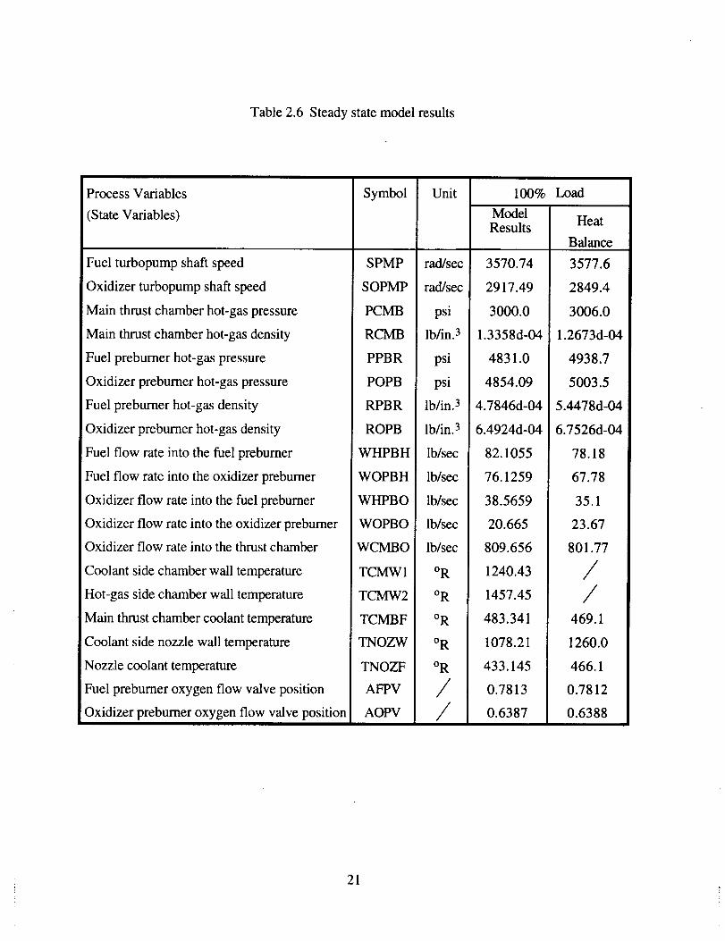
Table 2.6 Steady state model results
Process Variables
(State Variables)
Fuel turbopump shaft speed
Oxidizer turbopump shaft speed
Main thrust chamber hot-gas pressure
Main thrust chamber hot-gas density
Fuel preburner hot-gas pressure
Oxidizer preburner hot-gas pressure
Fuel preburner hot-gas density
Oxidizer preburner hot-gas density
Fuel flow rate into the fuel preburner
100% LoadSymbol Unit
ModelResults
Fuel flow rate into the oxidizer preburner
Oxidizer flow rate into the fuel preburner
Oxidizer flow rate into the oxidizer prebumer
Oxidizer flow rate into the thrust chamber
Coolant side chamber wall temperature
Hot-gas side chamber wall temperature
Main thrust chamber coolant temperature
Coolant side nozzle wall temperature
Nozzle coolant temperature
Fuel preburner oxygen flow valve position
Oxidizer prebumer oxygen flow valve position
SPMP
SOPMP
PCMB
RCMB
PPBR
POPB
RPBR
ROPB
WHPBH
rad/sec
rad/sec
psi
lb/in. 3
psi
psi
lb/in. 3
lb/in. 3
Ib/sec
3570.74
2917.49
3000.0
1.3358d-04
4831.0
4854.09
4.7846d-04
6.4924d-04
82.1055
WOPBH
WHPBO
WOPBO
WCMBO
TCMWl
TCMW2
TCMBF
TNOZW
TNOZF
AFPV
AOPV
lb/sec
lb/sec
lb/sec
lb/sec
o R
oR
oR
oR
oR
//
76.1259
38.5659
20.665
809.656
1240.43
1457.45
483.341
1078.21
433.145
0.7813
0.6387
Heat
Balance
3577.6
2849.4
3006.0
1.2673d-04
4938.7
5003.5
5.4478d-04
6.7526d-04
78.18
67.78
35.1
23.67
801.77
//
469.1
1260.0
466.1
0.7812
0.6388
21
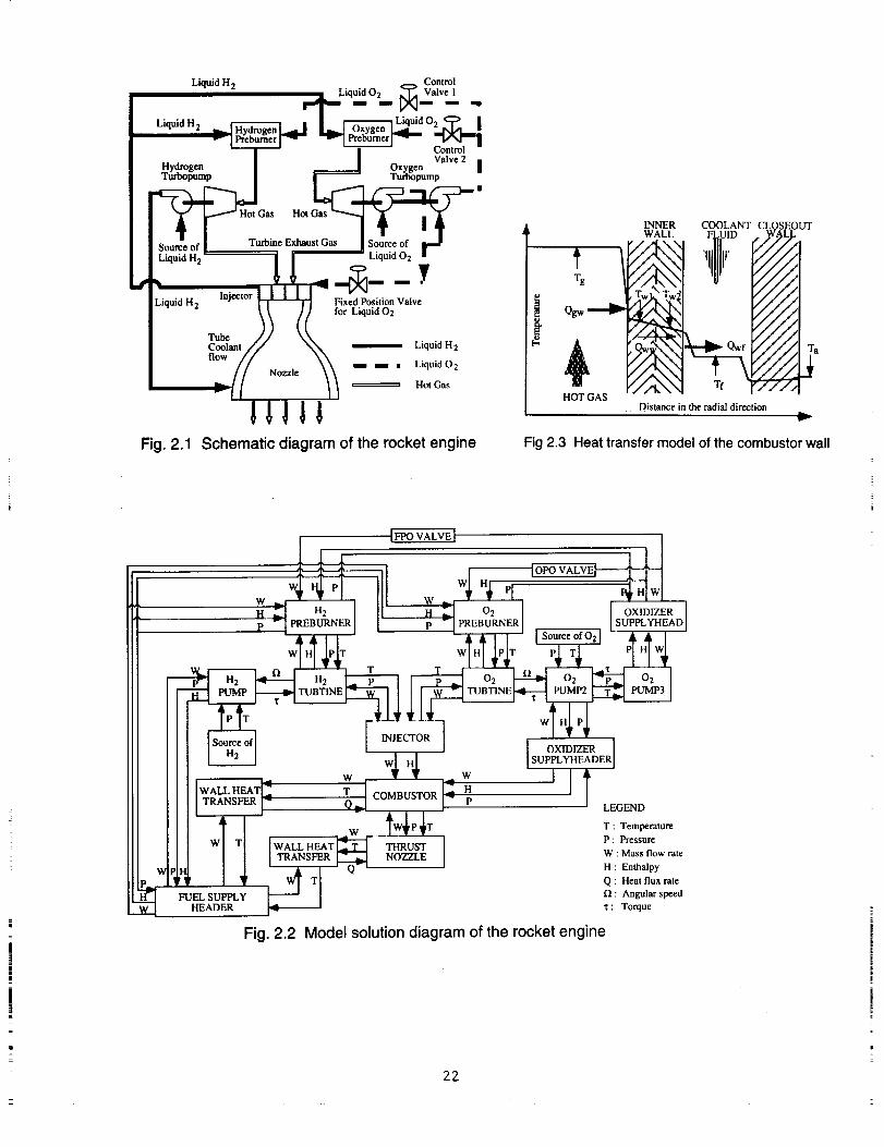
Liquid H_ __ Control- Liquid 02 _ Valve 1
,-'p.- - -N- - -Liquid H2 _ Pre LiquidO2__l. I
Hydrog¢ _ _ Oxygen mTurbopump _ _ Turbopump •
I so,SoofI Tu,bineE,_us,_as ISou_.02 ra
2_ l_ Llqul°l l YU2 •
Liquid H 2 "" .... _ Fixed Position Valve
- " _ (( for Liquid 02Tube I I \\Coolant // _ _ Liquid H 2flow / / \X
// .o,zle\\---" Liqo,dO,_{[ II _ .o,Oas
Fig. 2.1 Schematic diagram of the rocket engine
HOT GAS
INNER
. .W2LL.
. MWW _. "%'
COOLANT CLOSEOUTFLUID WALL
'l r
/_//
ffJ//
/_//
/_//
fj#l
,f _
Distance in the radial direction
Fig 2.3 Heat transfer model of the combustor wall
w
[FPOVALVE]
[OPO VALVEW
H2 02
PREBURNER p PREBURNERSource of 02
OXIDIZERSUPPLYHEAD
AAI,_1 HI WI
T
I I I
TRANSFER
FUEL SUPPLYHEADER
INJECTOROXIDIZER
W SUPPLYHEADER
W W
T COMBUSTOR HP
LEGEND
T : Temperature
P : PressureWALL HEAT THRUSTTRANSFER NOZZLE W : Mass flow rate
H : Enthalpy
Q : Heat flux rate
fl : Angular speed
•t : Torque
Fig. 2.2 Model solution diagram of the rocket engine
22
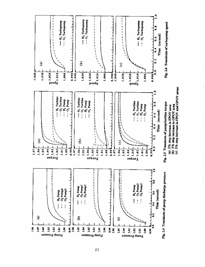
I: BS
o
paad S a paad S
" II _- _ _
I ; ,,
_" V'" ._ '_
'K-, d __._.-.... z "-"" """"" :1f I ! i ! I l, I I l [_
_nb:_oj_ _nb._o X _nbJoj_ .._
i,
i:
_. I ;
\%1,
I I 1 I I I
o.mssoa_l dmnd
' :' 1i I: I '
' I' Gi_ _, i_.,
': ',', _6'_ "_6'_ ,: ,
'Ii [" I,
ozns'so_ d dmn d _znssoz d dmn d
23

L..
ij+I': o
!
I"
I"
I"
I-I"
I"
I"
r
I"
I •
I"
4-
I-
i,
I,
I -J
I I I I -
i.-_-+I * I'I,
[ i, , ;'_ , ..] I I I
• , • • . .
L,
I...*
1=
[,-,<
e,.1
, l, 1 , I ,1 , ,-
iltl
I I 1 I
24
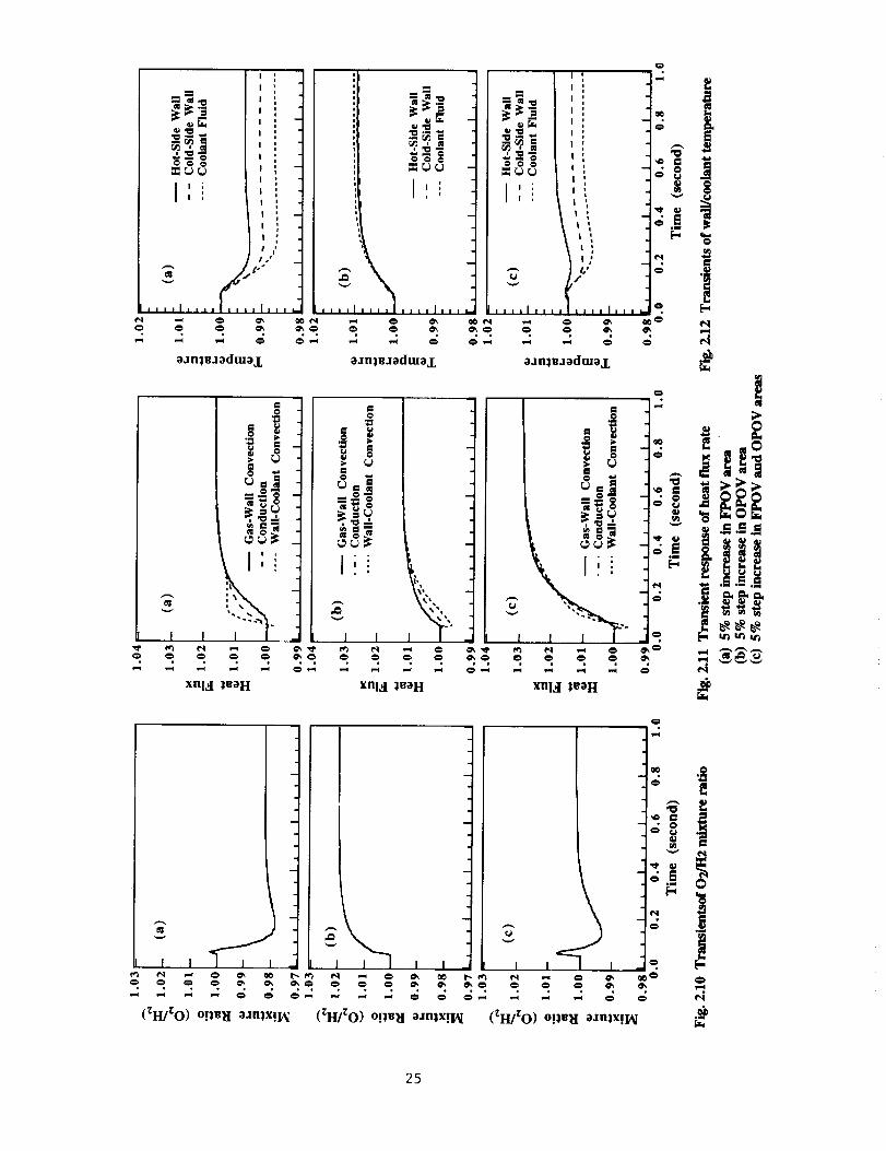
25
CHAPTER 3
STRUCTURAL AND DAMAGE MODELS OF THE REUSABLE ROCKET ENGINE
The critical components of the reusable rocket engine under consideration, which couldsignificantly reduce its service life, include (see Fig. 2. I):
• Blades of the fuel turbine;
• Blades of the oxidizer turbine;• Main thrust chamber coolant channel ligaments cooled by liquid hydrogen;• Rocket nozzle coolant channel ligaments cooled by liquid hydrogen;• Injector tubes carrying the turbine exhaust gas into the combustion chamber.
The fatigue failure in the injector tubes, originally caused by thermal stresses, has beensolved by appropriate selection of materials in the later versions of the Space Shuttle MainEngine (SSME). Therefore, the injector tube is not included as a critical point in the presentstudy. The failure of coolant channel ligaments (i.e., walls of the coolant channel) in the mainthrust chamber and rocket nozzle is caused by creep and creep ratcheting due to plasticity at high
temperatures (for example, in the vicinity of i200OR). Since the heat flux through the coolantchannel ligament at the throat section of the main thrust chamber is higher than that at othersections of the nozzle, the damage control of the coolant channel ligament in the main thrustchamber is expected to protect the nozzle coolant wall. Therefore, the first three components,namely, blades of the fuel turbine, blades of the oxidizer turbine, and coolant channel ligamentsat the main thrust chamber are selected as the critical points for damage mitigating control. Thedamage model is a representation of:
• Fatigue at the roots of the fuel and oxidizer turbine blades, and• Creep and creep ratcheting of the coolant channel ligaments at the throat plane of the
main thrust chamber.
3.1 Structural and Damage Model of the Turbine Blades
The structural model in each of the fuel and oxidizer turbines calculates the cyclicmechanical stresses at the root of a typical blade which is presumed to be a critical point in thisdissertation. The blade model for each of the two turbines is represented by a three-node beammodel with six degrees of freedom at each node while the first node at the root is fixed. The loadon each blade model is assumed to consist of two components, namely, the (time-dependent)drive torque, and the oscillatory load on the blade as it passes each stator. It is the secondcomponent that causes high cycle fatigue at the root of the blade while the first component islargely responsible for the mean stress. The resulting stiffness matrix, mass matrix, and forcevector are used to obtain a model solution for the displacements. In the last step, the stress-
displacemen t relations from the linear elastic finite element analysis are used to predict thestresses at the critical point(s) of the blade structure.
The development of this fatigue damage model is reported in detail by Ray et al. (1994a)
and Ray and Wu (1994a, 1994b) by assuming the damage rate dS/dt is obtained as theweighted average of the elastic and plastic damage rates such that
d..._ = w dS_____e+ (1 _ w) dSpdt dt dt (3.1)
where the weighting function, w, is selected as the ratio of the elastic strain amplitude and totalstrain amplitude. Since the turbine blades are subjected to loads of varying amplitude, the lineardamage is modified via a nonlinear damage rule as follows:
26
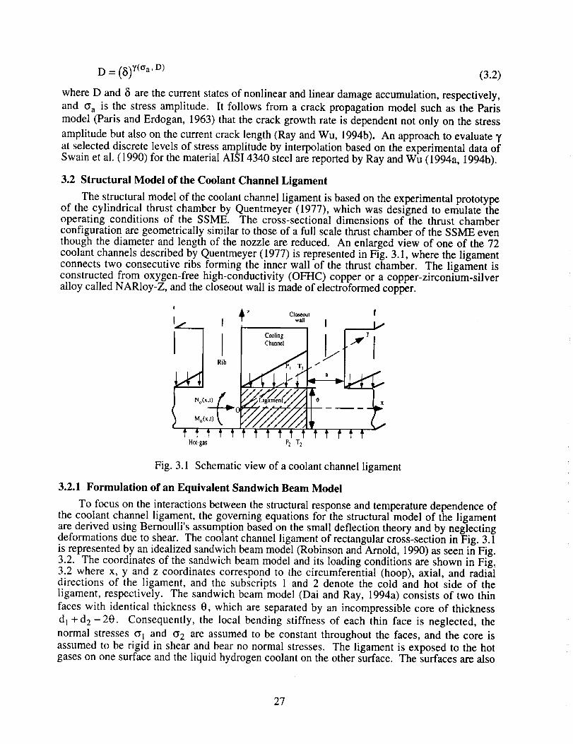
D=(Sf t(%'D) (3.2)
where D and 5 are the current states of nonlinear and linear damage accumulation, respectively,
and c_a is the stress amplitude. It follows from a crack propagation model such as the Paris
model (Paris and Erdogan, 1963) that the crack growth rate is dependent not only on the stress
amplitude but also on the current crack length (Ray and Wu, 1994b). An approach to evaluate _,
at selected discrete levels of stress amplitude by interpolation based on the experimental data ofSwain et al. (1990) for the material AIS14340 steel are reported by Ray and Wu (1994a, 1994b).
3.2 Structural Model of the Coolant Channel Ligament
The structural model of the coolant channel ligament is based on the experimental prototypeof the cylindrical thrust chamber by Quentmeyer (1977), which was designed to emulate theoperating conditions of the SSME. The cross-sectional dimensions of the thrust chamberconfiguration are geometrically similar to those of a full scale thrust chamber of the SSME even
though the diameter and length of the nozzle are reduced. An enlarged view of one of the 72coolant channels described by Quentmeyer (1977) is represented in Fig. 3.1, where the ligamentconnects two consecutive ribs forming the inner wall of the thrust chamber. The ligament isconstructed from oxygen-free high-conductivity (OFHC) copper or a copper-zirconium-silveralloy called NARloy-Z, and the closeout wall is made of electroformed copper.
i A z Closeout
I I T w_l
iL_l i "-Cooling--
1 Rib
I r_
Hot-gas P2 T2
!
Fig. 3.1 Schematic view of a coolant channel ligament
3.2.1 Formulation of an Equivalent Sandwich Beam Model
To focus on the interactions between the structural response and temperature dependence ofthe coolant channel ligament, the governing equations for the structural model of the ligamentare derived using Bernoulli's assumption based on the small deflection theory and by neglectingdeformations due to shear. The coolant channel ligament of rectangular cross-section in Fig. 3.1is represented by an idealized sandwich beam model (Robinson and Arnold, 1990) as seen in Fig.3.2. The coordinates of the sandwich beam model and its loading conditions are shown in Fig,3.2 where x, y and z coordinates correspond to the circumferential (hoop), axial, and radialdirections of the ligament, and the subscripts I and 2 denote the cold and hot side of theligament, respectively. The sandwich beam model (Dai and Ray, 1994a) consists of two thin
faces with identical thickness 0, which are separated by an incompressible core of thickness
d I +d 2 -20. Consequently, the local bending stiffness of each thin face is neglected, the
normal stresses cr! and t_ 2 are assumed to be constant throughout the faces, and the core is
assumed to be rigid in shear and bear no normal stresses. The ligament is exposed to the hotgases on one surface and the liquid hydrogen coolant on the other surface. The surfaces are also
27
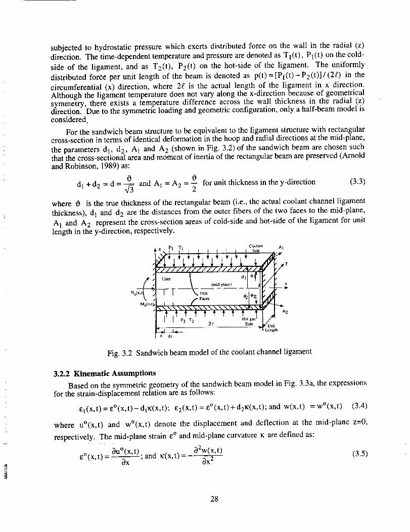
subjectedto hydrostatic pressurewhich exertsdistributed force on the wall in the radial (z)direction. The time-dependenttemperatureandpressurearedenotedasTl(t ), Pl(t) on thecold-side of the ligament, and as T2(t), P2(t) on the hot-side of the ligament. The uniformlydistributed force per unit length of the beamis denotedas p(t)= [Pl(t)-P2(t)]/(2g) in thecircumferential (x) direction, where 2g is the actual length of the ligament in x direction.Although the ligamenttemperaturedoesnot vary alongthe x-directionbecauseof geometricalsymmetry, there exists a temperaturedifference acrossthe wall thicknessin the radial (z)direction. Dueto thesymmetricloadingandgeometricconfiguration,only ahalf-beammodel isconsidered.
For thesandwichbeamstructureto beequivalentto the ligament structure with rectangularcross-section in terms of identical deformation in the hoop and radial directions at the mid-plane,
the parameters d 1, d 2 , A 1 and A 2 (shown in Fig. 3.2) of the sandwich beam are chosen suchthat the cross-sectional area and moment of inertia of the rectangular beam are preserved (Arnoldand Robinson, 1989) as:
0 0
d I + d 2 = d = -_ and A 1 = A 2 = --2 for unit thickness in the y-direction (3.3)
where 0 is the true thickness of the rectangular beam (i.e., the actual coolant channel ligament
thickness), d 1 and d 2 are the distances from the outer fibers of the two faces to the mid-plane,
A 1 and A 2 represent the cross-section areas of cold-side and hot-side of the ligament for unit
length in the y-direction, respectively.
z PI TI
• ll////l//////ti//_a
Core d 1
(._._____idzrl_'e.._._2__)_No(X,t
Mo(x,Q,
Coolant A I
//_
-- -- IP
-V 1-F_:_s aZ Oe1f
1 / /\\ \'\\\\\\\\\\\\ \ \",d \\
P2 T2
2 t Side UnitLength
x dx
Fig. 3.2 Sandwich beam model of the coolant channel ligament
3.2.2 Kinematic Assumptions
Based on the symmetric geometry of the sandwich beam model in Fig. 3.3a, the expressionsfor the strain-displacement relation are as follows:
El(x,t)=E°(x,t)-d_z(x,t); E2(x,t)=_°(x,t)+d2tc(x,t); and w(x,t) =w°(x,t) (3.4)
where u°(x,t) and w°(x,t) denote the displacement and deflection at the mid-plane z=0,
respectively. The mid-plane strain _o and mid-plane curvature tz are defined as:
E°(x,t) = _u°(x't)" and _:(x,t)= _2w(x't) (3.5)_x ' _x 2
28
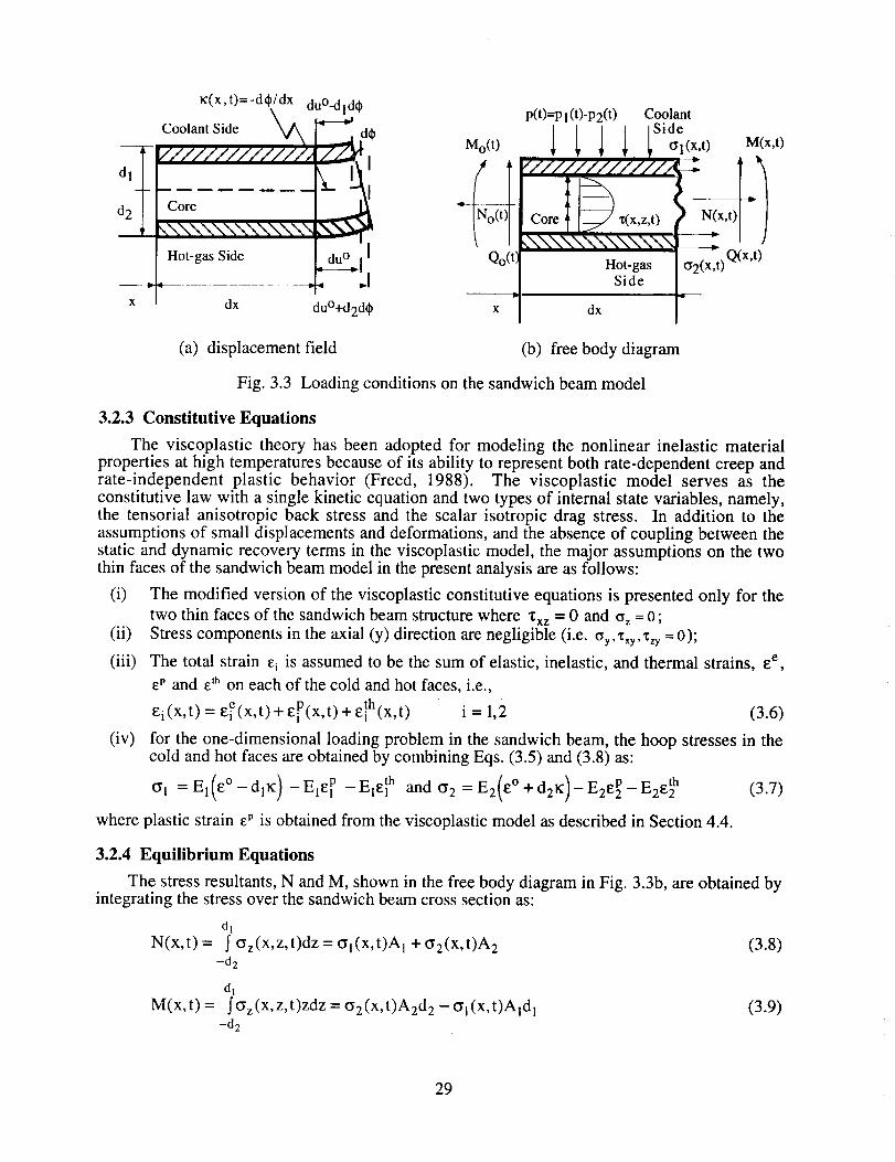
L_
x
_(x,t)=-d#/dx
Core
Hot-gas Side
dx
du°-d !dd_
du°+d2d#
p(t)=p i (t)-P2(t)
Mo(t) 1
Coolant
]Side_ 1 _ Ol(X,t) M(x,t)
,t)
Hot gas o2(x,t) Q(,t)Side
dx
(a) displacement field (b) free body diagram
Fig. 3.3 Loading conditions on the sandwich beam model
3.2.3 Constitutive Equations
The viscoplastic theory has been adopted for modeling the nonlinear inelastic materialproperties at high temperatures because of its ability to represent both rate-dependent creep andrate-independent plastic behavior (Freed, 1988). The viscoplastic model serves as theconstitutive law with a single kinetic equation and two types of internal state variables, namely,the tensorial anisotropic back stress and the scalar isotropic drag stress. In addition to theassumptions of small displacements and deformations, and the absence of coupling between thestatic and dynamic recovery terms in the viscoplastic model, the major assumptions on the twothin faces of the sandwich beam model in the present analysis are as follows:
(i) The modified version of the viscoplastic constitutive equations is presented only for the
two thin faces of the sandwich beam structure where 'Cxz = 0 and oz = 0 ;
(ii) Stress components in the axial (y) direction are negligible (i.e. %,%,% = 0);
(iii) The total strain e_ is assumed to be the sum of elastic, inelastic, and thermal strains, e e,
Ep and e_ on each of the cold and hot faces, i.e.,
_;i(x,t) = ee(x,t) + eiP(x,t) + e[h(x,t) i = 1,2 (3.6)
(iv) for the one-dimensional loading problem in the sandwich beam, the hoop stresses in thecold and hot faces are obtained by combining Eqs. (3.5) and (3.8) as:
G l = El(_°-dj_:) -Eiel p -EIEI h and G 2 = E2(£ ° +d2K)-E2EP-E2£_ h (3.7)
where plastic strain eP is obtained from the viscoplastic model as described in Section 4.4.
3.2.4 Equilibrium Equations
The stress resultants, N and M, shown in the free body diagram in Fig. 3.3b, are obtained byintegrating the stress over the sandwich beam cross section as:
dl
N(x,t) = _ az(X,Z,t)dz = ffl(x,t)A1 + G2(x,t)A2 (3.8)-d 2
dl
M(x,t) = _Oz(X,z,t)zdz = o2(x,t)A2d 2 - Gl(x,t)AId l-d 2
(3.9)
29
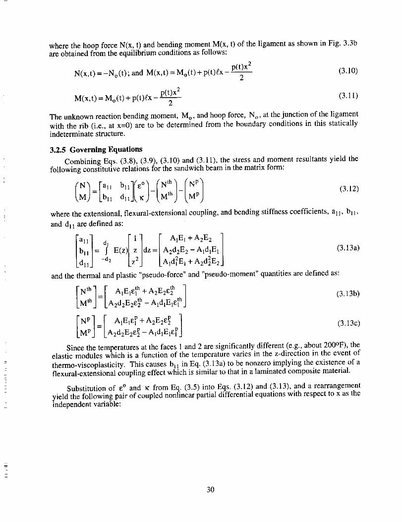
where the hoop force N(x, t) and bending moment M(x, t) of the ligament as shown in Fig. 3.3bare obtained from the equilibrium conditions as follows:
N(x,t) = -No(t); and M(x,t) = Mo(t) + p(t)gx
M(x,t) = Mo(t)+ p(t)gx P(t)x22
p(t)x 2
2(3.10)
(3.11)
The unknown reaction bending moment, M o , and hoop force, N o, at the junction of the ligament
with the rib (i.e., at x=0) are to be determined from the boundary conditions in this staticallyindeterminate structure.
3.2.5 Governing Equations
Combining Eqs. (3.8), (3.9), (3.10) and (3.11), the stress and moment resultants yield thefollowing constitutive relations for the sandwich beam in the matrix form:
blll(E°_- INth ]- ( Np ]Lb,, d,,J__) _.M 'h M p(3.12)
where the extensional, flexural-extensional coupling, and bending stiffness coefficients, all, b I x,
and dll are defined as:
a'l d_ I 1] I A1E.+A2E2
bll = I E(z) / z ]dz=lA2d2E2-AldlE ldll -d2 Lz2J LA,O, E,+A20 E2
and the thermal and plastic "pseudo-force" and "pseudo-moment" quantities are defined as:
Nth]:[ A,EIEI"+A=E26h ]Mth.J LA2dEE2E_h-AldlEl_lhj
Mp LA2d2E2eP- A,O,E1el'J
(3.13a)
(3.13b)
(3.13c)
Since the temperatures at the faces 1 and 2 are significantly different (e.g., about 200°F), theelastic modules which is a function of the temperature varies in the z-direction in the event of
thermo-viscoplasticity. This causes bll in Eq. (3.13a) to be nonzero implying the existence of aflexural-extensional coupling effect which is similar to that in a laminated composite material.
Substitution of e ° and r from Eq. (3,5) into Eqs, (3.12) and (3.13), and a rearrangementyield the following pair of coupled nonlinear partial differential equations with respect to x as theindependent variable:
30
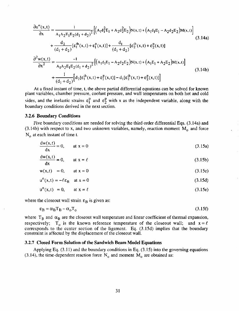
Ou°(x,t)
_x_ 1 [(Ald2EI + A2d2E2)N(x,t)+ (AldlEI- A2d2E2)M(x, t)]
AIA2E1E2(d 1 + d2 )2
+
b2w(x,t)
82
(d 1 + d 2)[elh(x,t)+eP(x,t)]+ .. dl .[etvh(x,t)+e2P(x,t)]
[,(11 +02 )
(3.14a)
-1 [(AldlE1- A2d2E2)N(x,t)+ (ALE1 + A2E2)M(x,t)]_X 2 AIA2E1E2(d 1 +d2 )2
(3.14b)1
__ retht x t) + eP(x,t)]]tO2[e h(x,t)+e,(x,t)] dl, ,-I: (dl + d2)
At a fixed instant of time, t, the above partial differential equations can be solved for knownplant variables, chamber pressure, coolant pressure, and wall temperatures on both hot and cold
sides, and the inelastic strains E1p and Ep with x as the independent variable, along with the
boundary conditions derived in the next section.
3.2.6 Boundary Conditions
Five boundary conditions are needed for solving the third order differential Eqs. (3.14a) and
(3.14b) with respect to x, and two unknown variables, namely, reaction moment M o and force
N O at each instant of time t.
dw(x,t)- 0, at x = 0 (3.15a)
dx
dw(x,t)-0, atx=g
dx
w(x,t) =0, atx=0
(3.15b)
(3.15c)
u°(x,t) =-ge a at x = 0 (3.15d)
u°(x,t) = 0, at x = g (3.15e)
where the closeout wall strain rB is given as:
_:B = °_BTB - °_oTo (3.15f)
where T B and czB are the closeout wall temperature and linear coefficient of thermal expansion,
respectively; T o is the known reference temperature of the closeout wall; and x = g
corresponds to the center section of the ligament. Eq. (3.15d) implies that the boundaryconstraint is affected by the displacement of the closeout wall.
3.2.7 Closed Form Solution of the Sandwich Beam Model Equations
Applying Eq. (3.11) and the boundary conditions in Eq. (3.15) into the governing equations
(3.14), the time-dependent reaction force N o and moment M o are obtained as:
31
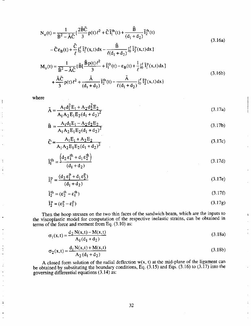
1 {_2__p(t),2 + (_i_h(t)+No(t) - f2 _ _ (dI + d2)I2th(t)
- (_ e B d2) fg i2P(x,t)dx }-CeB(t)+_-I 6 iP(x,t)dx g(dl +
Mo(t)= 1 {_[fp(t)g 2fiE-he 3 + i_h (t) - eB(t) + I g ip (x,t)dx ]
_. N i th(t)+--_p(t)g 2 -t (dl +d2) "_ d2 ) _oei2P(x,t)dx}
g(d 1 +
(3.16a)
(3.16b)
where
,_= Ald2EI+A2d2E2
A1A2E1E2(dl + d2) 2
AldlE 1 - A2d2E2f
A1A2E1E2(d 1 +d2) 2
A1EI + A2E 2
AI A2EI E2(dl + d2) 2
_{h = ( d2 e_h + dl e_h)
(d 1 + d 2)
(3.17a)
(3.17b)
(3.17c)
(3.17d)
]1p = (d2 elp + d 1 e p)(d 1 + d 2)
(3.17e)
(3.170
(3.17g)
Then the hoop stresses on the two thin faces of the sandwich beam, which are the inputs to
the viscoplastic model for computation of the respective inelastic strains, can be obtained interms of the force and moment from Eq. (3.10) as:
(_l(x,t) = d 2 N(x,t) - M(x,t) (3.18a)Al (dl + d e)
(_2(x,t) = d 1N(x,t) + M(x,t) (3.18b)A 2 (d! + d2)
A closed form solution of the radial deflection w(x, t) at the mid-plane of the ligament can
be obtained by substituting the boundary conditions, Eq. (3.15) and Eqs. (3.16) to (3.17) into the
governing differential equations (3.14) as:
32
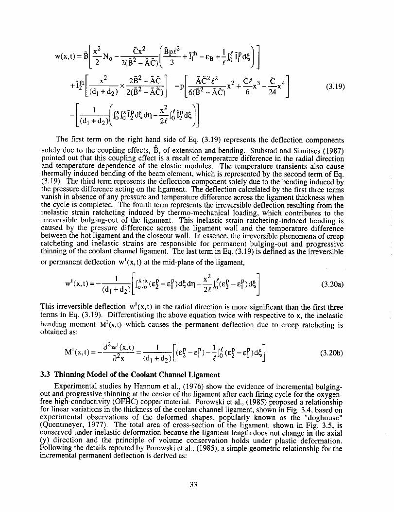
Ix 2 (2x2 (Bpg2 _ h 1 g )]Trio -EB+Tf ilPO
-P[6(_2 _ _(_ ) -Cx4
[ ( x2 rg TPd/_)]1 fx fxiPd_dTl_.__jO, 2 -_(d l+d2) JOJ012
(3.19)
The first term on the right hand side of Eq. (3.19) represents the deflection components
solely due to the coupling effects, B, of extension and bending. Stubstad and Simitses (1987)pointed out that this coupling effect is a result of temperature difference in the radial directionand temperature dependence of the elastic modules. The temperature transients also cause
thermally induced bending of the beam element, which is represented by the second term of Eq.(3.19). The third term represents the deflection component solely due to the bending induced bythe pressure difference acting on the ligament. The deflection calculated by the first three terms
vanish in absence of any pressure and temperature difference across the ligament thickness whenthe cycle is completed. The fourth term represents the irreversible deflection resulting from theinelastic strain ratcheting induced by thermo-mechanical loading, which contributes to the
irreversible bulging-out of the ligament. This inelastic strain ratcheting-induced bending iscaused by the pressure difference across the ligament wall and the temperature difference
between the hot ligament and the closeout wall. In essence, the irreversible phenomena of creepratcheting and inelastic strains are responsible for permanent bulging-out and progressivethinning of the coolant channel ligament. The last term in Eq. (3.19) is defined as the irreversible
or permanent deflection w _(x, t) at the mid-plane of the ligament,
wi xt) ]= - Io(e2 - eP)d_ (3.20a)(dl d2) drl _
This irreversible deflection w_(x,t) in the radial direction is more significant than the first three
terms in Eq. (3.19). Differentiating the above equation twice with respective to x, the inelastic
bending moment M_(x,t) which causes the permanent deflection due to creep ratcheting isobtained as:
M'(x,t) = _2w'(x't) 1 [(eP - _P)- 1.[_ (EP - eP)d_]_2 x = (d 1 + d 2)(3.20b)
3.3 Thinning Model of the Coolant Channel Ligament
Experimental studies by Hannum et al., (1976) show the evidence of incremental bulging-out and progressive thinning at the center of the ligament after each firing cycle for the oxygen-free high-conductivity (OFHC) copper material. Porowski et al., (1985) proposed a relationshipfor linear variations in the thickness of the coolant channel ligament, shown in Fig. 3.4, based onexperimental observations of the deformed shapes, popularly known as the "doghouse"(Quentmeyer, 1977). The total area of cross-section of the ligament, shown in Fig. 3.5, isconserved under inelastic deformation because the ligament length does not change in the axial(y) direction and the principle of volume conservation holds under plastic deformation.Following the details reported by Porowski et al., (I 985), a simple geometric relationship for theincremental permanent deflection is derived as:
33

l gsl(t)=l (g +4)wI(t)=l (g +2)8:(t) (3.21)
where 81 and 82 are denoted as the respective deflections of the cold-side face and hot-side face
at the center of the ligament; and a is the rib width in the coolant channel. The time-dependent
thinning, x(t), of the ligament at its center is obtained as:
x(t) = 81(t) - 82(0 = w(t)(4g + a)a (3.22)4e(2g + a)
and the normalized thinning, _(t), relative to the initial ligament thickness, Oo, is obtained as:
_(t) = 'r(t) / Oo (3.23)
and the creep damage of the coolant channel ligament is defined as:
Dcr (t) = _(t) / "_* (3.24)
where "c*is the critical thinning at which the bulging process becomes unstable leading to tensile
rupture. The critical thinning of the ligament, x*, is different for different material. For
example, x* is about 0'37 for OFHC copper (Porowski et al., 1985) and is in the range of 0.05 to0.08 for NARloy-Z (Kasper, 1984).
I II
[ ' [ CloseOUtwall
I I
CoolingChannel
Hot-gas Side
X
Figure 3.4 Linear thinning model of the coolant channel ligament
The instantaneous thickness of the deformed beam is updated by subtracting the time-dependent thinning from the original thickness:
O(t) = O 0 - "c(t) (3.25)
Following Fig. 3.5, this information is fed back to the sandwich model in Eq. (3.3).
34
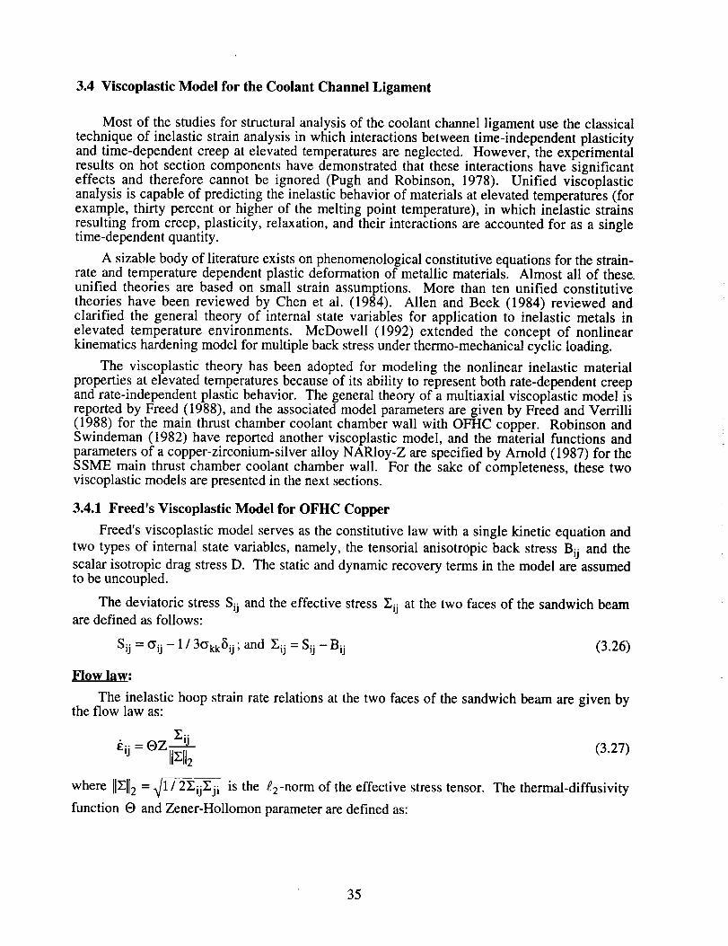
3.4 Viscoplastic Model for the Coolant Channel Ligament
Most of the studies for structural analysis of the coolant channel ligament use the classicaltechnique of inelastic strain analysis in which interactions between time-independent plasticityand time-dependent creep at elevated temperatures are neglected. However, the experimentalresults on hot section components have demonstrated that these interactions have significanteffects and therefore cannot be ignored (Pugh and Robinson, 1978). Unified viscoplasticanalysis is capable of predicting the inelastic behavior of materials at elevated temperatures (forexample, thirty percent or higher of the melting point temperature), in which inelastic strainsresulting from creep, plasticity, relaxation, and their interactions are accounted for as a singletime-dependent quantity.
A sizable body of literature exists on phenomenological constitutive equations for the strain-rate and temperature dependent plastic deformation of metallic materials. Almost all of these.unified theories are based on small strain assumptions. More than ten unified constitutivetheories have been reviewed by Chen et al. (1984). Allen and Beek (1984) reviewed and
clarified the general theory of internal state variables for application to inelastic metals inelevated temperature environments. McDowell (1992) extended the concept of nonlinearkinematics hardening model for multiple back stress under thermo-mechanical cyclic loading.
The viscoplastic theory has been adopted for modeling the nonlinear inelastic materialproperties at elevated temperatures because of its ability to represent both rate-dependent creepand rate-independent plastic behavior. The general theory of a multiaxial viscoplastic model isreported by Freed (1988), and the associated model parameters are given by Freed and Verrilli(1988) for the main thrust chamber coolant chamber wall with OFHC copper. Robinson andSwindeman (1982) have reported another viscoplastic model, and the material functions andparameters of a copper-zirconium-silver alloy NARloy-Z are specified by Arnold (1987) for theSSME main thrust chamber coolant chamber wall. For the sake of completeness, these twoviscoplastic models are presented in the next sections.
3.4.1 Freed's Viscoplastic Model for OFHC Copper
Freed's viscoplastic model serves as the constitutive law with a single kinetic equation and
two types of internal state variables, namely, the tensorial anisotropic back stress Bij and the
scalar isotropic drag stress D. The static and dynamic recovery terms in the model are assumedto be uncoupled.
The deviatoric stress Sij and the effective stress Eij at the two faces of the sandwich beamare defined as follows:
Sij -- (Yij - 1 / 3Okk_ij ; and Eij = Sij - Bij (3.26)
Flow law:
The inelastic hoop strain rate relations at the two faces of the sandwich beam are given bythe flow law as:
£ij
_ij --o211::112 (3.27)
where IlZl12= _/1 / 2EijEji is the g2-norm of the effective stress tensor. The thermal-diffusivity
function O and Zener-Hollomon parameter are defined as:
35
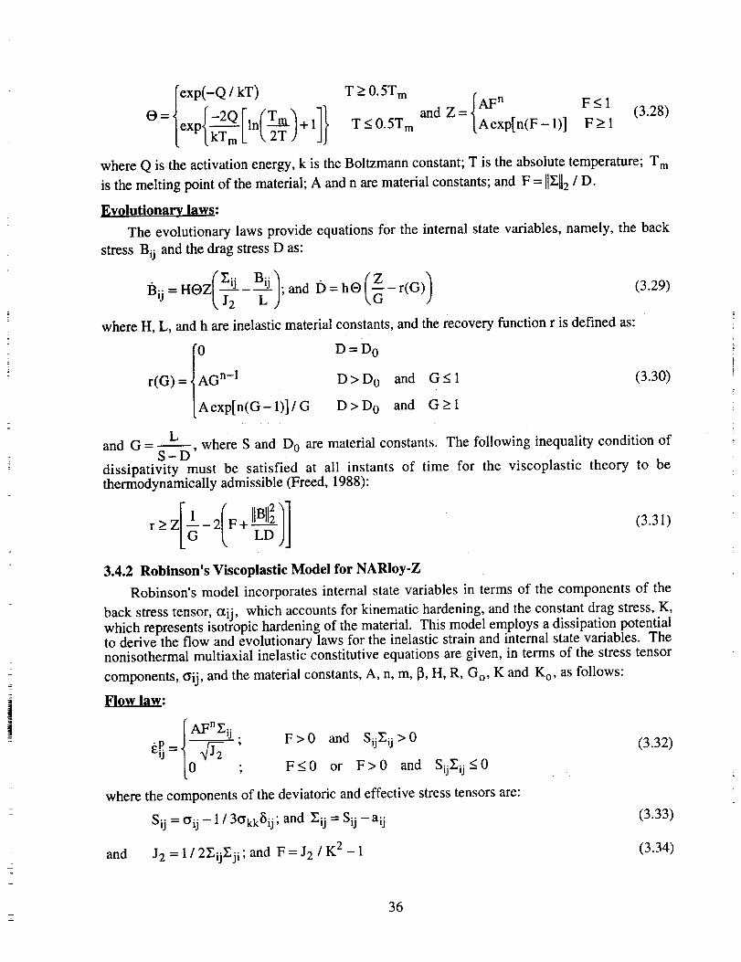
fll[exp(-Q/ kT) T > 0.5T m and Z= I AFn F < 1
O=lexp'_-2QIln(Tm_+lJl T<0.5Tm (Aexp[n(F-1)] F>I
(3.28)
l [ kTm L \ 2T J
where Q is the activation energy, k is the Boltzmann constant; T is the absolute temperature; T m
is the melting point of the material; A and n are material constants; and F = Ilxl12/ D.
Evolutionary_ laws:
The evolutionary laws provide equations for the internal state variables, namely, the back
stress Bij and the drag stress D as:
13ij = HOZ L ; and I3 = h O - r(G) (3.29)
where H, L, and h are inelastic material constants, and the recovery function r is defined as:
0 D = D Or(G)= AG n-I D>D O and G<I (3.30)
[Aexp[n(G-1)]/G D>D 0 and G>I
Land G = _, where S and D O are material constants. The following inequality condition of
S-D
dissipativity must be satisfied at all instants of time for the viscoplastic theory to bethermodynamically admissible (Freed, 1988):
(3.31)
3.4.2 Robinson's Viscoplastic Model for NARIoy-Z
Robinson's model incorporates internal state variables in terms of the components of the
back stress tensor,, oq',j which, accounts for kinematic hardening, and the constant drag stress, K,which represents lsotroplc hardening of the material. This model employs a dissipation potentialto derive the flow and evolutionary laws for the inelastic strain and internal state variables. Thenonisothermal multiaxial inelastic constitutive equations are given, in terms of the stress tensor
components, _ij, and the material constants, A, n, m, 1_,H, R, G o, K and K o, as follows:
Flow law:
f-mFnzij " F > 0 and SijZij > 0
1 '0 , F<0 or F>0 and SijEij < 0
where the components of the deviatoric and effective stress tensors are:
Sij = oij - 1 / 3Okk_Sij; and Zij = Sij - aij
(3.32)
(3.33)
and J2 = 1 / 2ZijZji ; and F = J2 / K2 - 1 (3.34)
36
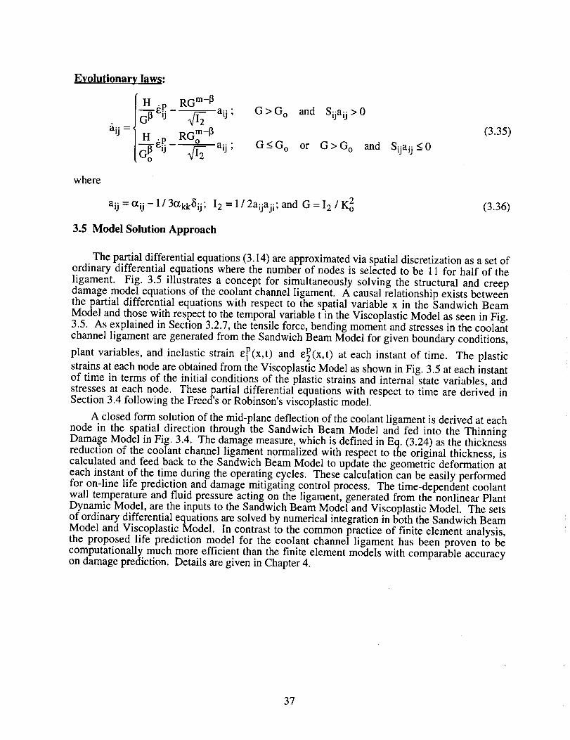
Evolutionary l_ws:
H .p RG m-13
_--ffsij _ aij ; G > G O and Sijaij > 0
RGm-I]aij; G<G o or G>G o and
aij =H.p
G_ 8iJSijaij < 0
(3.35)
where
aij = otij - 1 / 3O_kkSij; 12 = 1 / 2aijaji; and G = 12 / K 2 (3.36)
3.5 Model Solution Approach
The partial differential equations (3.14) are approximated via spatial discretization as a set ofordinary differential equations where the number of nodes is selected to be 11 for half of the
ligament. Fig. 3.5 illustrates a concept for simultaneously solving the structural and creepdamage model equations of the coolant channel ligament. A causal relationship exists betweenthe partial differential equations with respect to the spatial variable x in the Sandwich Beam
Model and those with respect to the temporal variable t in the Viscoplastic Model as seen in Fig.3.5. As explained in Section 3.2.7, the tensile force, bending moment and stresses in the coolant
channel ligament are generated from the Sandwich Beam Model for given boundary conditions,
plant variables, and inelastic strain 81P(x,t) and 8P(x,t) at each instant of time. The plastic
strains at each node are obtained from the Viscoplastic Model as shown in Fig. 3.5 at each instantof time in terms of the initial conditions of the plastic strains and internal state variables, andstresses at each node. These partial differential equations with respect to time are derived inSection 3.4 following the Freed's or Robinson's viscoplastic model.
A closed form solution of the mid-plane deflection of the coolant ligament is derived at eachnode in the spatial direction through the Sandwich Beam Model and fed into the ThinningDamage Model in Fig. 3.4. The damage measure, which is defined in Eq. (3.24) as the thicknessreduction of the coolant channel ligament normalized with respect to the original thickness, iscalculated and feed back to the Sandwich Beam Model to update the geometric deformation ateach instant of the time during the operating cycles. These calculation can be easily performedfor on-line life prediction and damage mitigating control process. The time-dependent coolantwall temperature and fluid pressure acting on the ligament, generated from the nonlinear PlantDynamic Model, are the inputs to the Sandwich Beam Model and Viscoplastic Model. The setsof ordinary differential equations are solved by numerical integration in both the Sandwich Beam
Model and Viscoplastic Model. In contrast to the common practice of finite element analysis,the proposed life prediction model for the coolant channel ligament has been proven to becomputationally much more efficient than the finite element models with comparable accuracyon damage prediction. Details are given in Chapter 4.
37
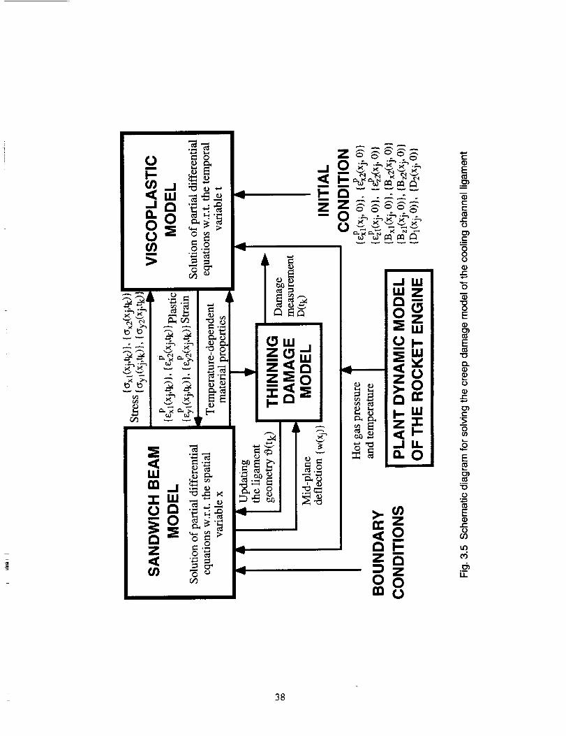
38
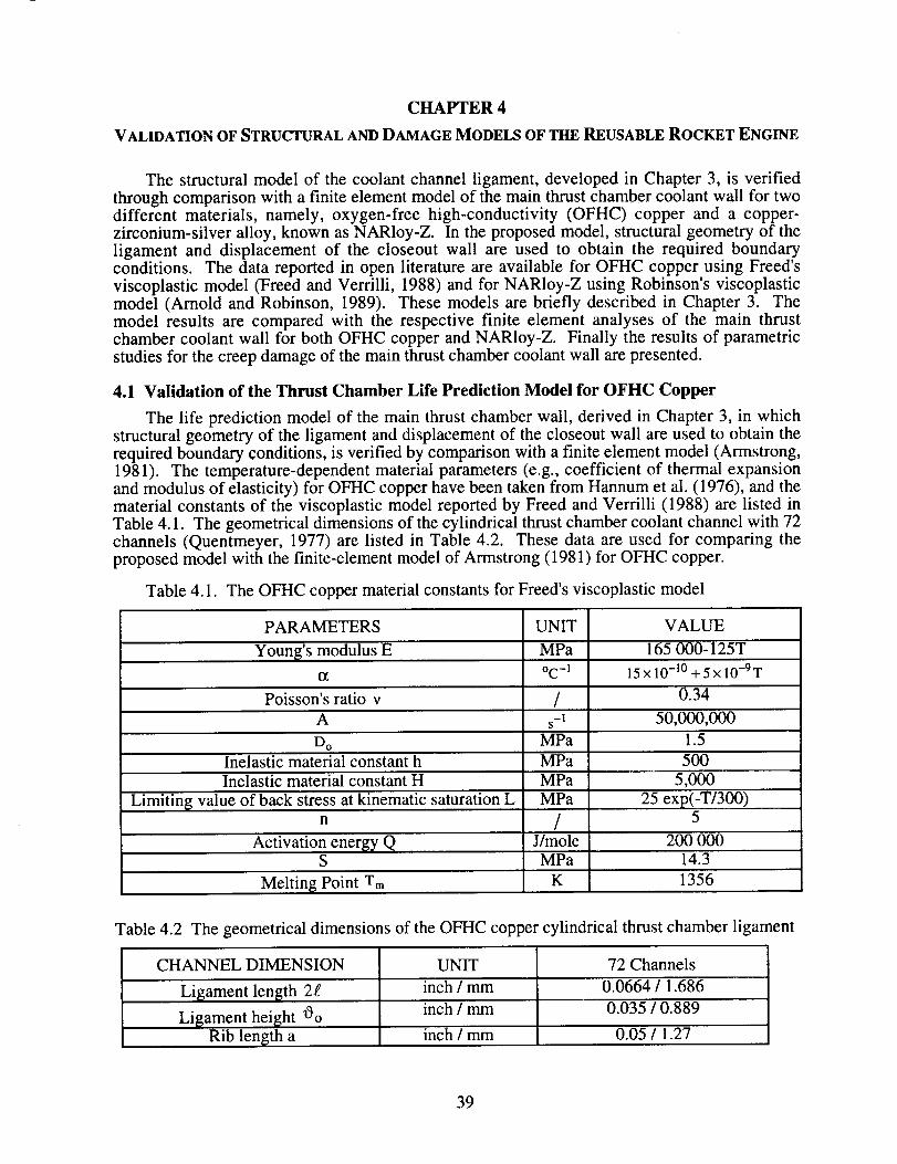
CHAPTER 4
VALIDATION OF STRUCTURAL AND DAMAGE MODELS OF THE REUSABLE ROCKET ENGINE
The structural model of the coolant channel ligament, developed in Chapter 3, is verified
through comparison with a finite element model of the main thrust chamber coolant wall for twodifferent materials, namely, oxygen-free high-conductivity (OFHC) copper and a copper-zirconium-silver alloy, known as NARloy-Z. In the proposed model, structural geometry of theligament and displacement of the closeout wall are used to obtain the required boundaryconditions. The data reported in open literature are available for OFHC copper using Freed's
viscoplastic model (Freed and Verrilli, 1988) and for NARIoy-Z using Robinson's viscoplasticmodel (Arnold and Robinson, 1989). These models are briefly described in Chapter 3. Themodel results are compared with the respective finite element analyses of the main thrustchamber coolant wall for both OFHC copper and NARIoy-Z. Finally the results of parametricstudies for the creep damage of the main thrust chamber coolant wall are presented.
4.1 Validation of the Thrust Chamber Life Prediction Model for OFHC Copper
The life prediction model of the main thrust chamber wail, derived in Chapter 3, in whichstructural geometry of the ligament and displacement of the closeout wall are used to obtain therequired boundary conditions, is verified by comparison with a finite element model (Armstrong,1981). The temperature-dependent material parameters (e.g., coefficient of thermal expansionand modulus of elasticity) for OFHC copper have been taken from Hannum et al. (1976), and thematerial constants of the viscoplastic model reported by Freed and Verrilli (1988) are listed inTable 4.1. The geometrical dimensions of the cylindrical thrust chamber coolant channel with 72channels (Quentmeyer, 1977) are listed in Table 4.2. These data are used for comparing theproposed model with the finite-element model of Armstrong (1981) for OFHC copper.
Table 4.1. The OFHC copper material constants for Freed's viscoplastic model
PARAMETERS UNIT VALUE
MPa 165 000-125TYoung's modulus E
0_
Poisson's ratio v
A
D O
Inelastic material constant h
Inelastic material constant H
Limitin_ value of back stress at kinematic saturation Ln
Activation energy Qs
Melting Point Tm
oc-1
-1S
MPa
MPa
MPa
MPa
J/mole
MPa
K
15x 10 -1° +5x 10⁻⁹T
0.34
50,000,000
1.5
500
5,000
25 exp(-T/300)
200 00014.3
1356
Table 4.2 The geometrical dimensions of the OFHC copper cylindrical thrust chamber ligament
CHANNEL DIMENSION
Ligament length 2g
Ligament height Oo
Rib length a
UNIT
inch / mm
inch / mm
inch / mm
72 Channels
0.0664/1.686
0.035/0.889
0.05 / 1.27
39
Fig. 4.1 showsthetime historyof theprocessvariables,namely, cold-sidewail temperature(T_), the hot-side wall temperature (T2), closeout wall temperature (TB), and the pressure loadacting on the ligament for a typical firing cycle having a duration of 3.5 seconds. These processvariables excite the structural and damage model as discussed in Chapter 3. The time period of3.5 seconds includes start-up and heating, referred to as the hot phase of a cycle, and shut-downand cooling, referred to as the cold phase of a cycle.
4.1.1 Single Cycle Behavior
Both temporal and spatial responses of the ligament structure are investigated for a typicalsingle cycle (i.e., the 3rd cycle in this simulation). Time histories of stress and strain of thesandwich beam model are presented in Fig. 4.2 for one firing cycle. As the temperature israpidly increased corresponding to the transient heating part of the firing cycle, the hoop stresschanges from tension to large compression due to the restricted expansion of the hot ligamentimposed by the relatively cool closeout wall which exhibits elastic behavior. Thus, during theheating process, large plastic compressive strains are induced in the ligament. The stressovershoot occurs at the instants of t=0.27 sec and 2.07 sec corresponding to the maximumtemperature difference between the Iigament and ci0seout Wall during the Cycle. For the coolingprocess, a similar situation occurs except that the closeout wall is at a higher temperature than thecoolant ligame-nfwhicti is subjected to _e rnaxim um tensile s_re_L AS the temperaturedifference between the ligament and the closeout wall diminishes in the cold phase of the cycle,which follows the minimum temperature difference attained during the shut-down process, thetensile stress induced by the inelastic strain in the ligament reduces from its maximum level.
During the hot phase of the cycle, the compressive stress generally decreases or relaxes afterthe peak and then tends to keep constant. When the ligament is exposed to a higher temperatureenvironment, the stress relaxation phenomenon becomes more significant. This behavior ischaracterized as the transition from "primary creep" to "secondary" or "steady" creep, and can beexplained in terms of the constitutive equations of viscoplasticity as discussed by Stubstad andSimitses (1987). An examination of the flow model of viscoplasticity described in Chapter 3reveals that the inelastic strain rate is determined by the effective stress, i.e., the differencebetween the actual stress and the back stress. The inelastic strain rate changes whenever the rateof the actual stress differs from that of the back stress. In some situations, however, the rates ofactual stress and back stress tend to have a constant difference, and the rate of inelastic strain
stabilizes to a constant value which is known as the secondary creep.
The shape of the predicted hoop stress and strain at the cold-side and hot-side ligament areshown in Figs. 4.3 and 4.4 at two specific instants of t[me, fiamely, t=i.7 and 3,4 seccorresponding to the end of the hot and cold phases of a typical cycle. The stress is tensilethroughout the ligament during the chill-down part of the cycle and compressive during theheating-up part as mentioned earlier. The shape of the predicted hoop stress distribution on thehot-side ligament is different from that on the cold-side as seen in Fig. 4.3. This difference ismore pronounced during the hot phase of a cycle (at t= 1.7 sec) than that during the cold phase (att=3.4 sec) because of a larger temperature difference between the ligament_andthe _!oseout wall,At the end of the cycle, the predicted tensile hoop stress differ¢.n_ i_h¢ radial direction is lessthan about 8 MPa throughout the Iigarnent length. The maximum h0op stress occurs at the centerof the hot-side ligament, which is in agreement with the results of finite element analysisreported by Arya (1992). The shape of the predicted inelastic strain distribution in the hoopdirection on the hot-side is different from that on the cold-side in Fig. 4.4. The maximum
effective strain range occurs on the hot-side at the center of the ligament. This is in agreementwith the experimental results reported by Hannum et al. (1976). The effective strain rangedistribution in the hoop direction can be calculated by taking the difference of the maximum andminimum inelastic strain within one firing cycle.
40
In orderto closelyexaminethefailuremechanismof thecoolantchanneldueto incremental
bulging-out, Figs. 4.5 and4.6 showthe irreversibledeflection wI(x,t) defined in Eq. (3.20a)which is normalizedwith respectto the initial thicknessof the ligament, Oo, and the inelastic
bending moment MI(t,x), defined in Eq. (3.20b), at the two instants t=l.7 and 3.4 sec
corresponding to the hot and cold phases of a cycle. Since the shape of the distribution of theinelastic strain difference between the hot and cold sides of the ligament is always convex as
seen from Fig. 4.4, the shape of MI(t,x) profile in Fig. 4.6 is also convex by virtue of the
relationship in Eq. (3.20b). This bending moment distribution implies progressive bulging-out ofthe coolant channel ligament in Fig. 4.5 during both hot and cold phases.
Time history of the associated normalized thinning _ at the ligament center, defined in Eq.(3.23a), is shown in Fig. 4.7 for a typical cycle where progressive thinning is observed. Therapid increase in ligament thinning occurs during the heat-up and chill-down transients. During athermo-mechanical loading transient, the back stress lags behind the actual stress. This results in
large rate of change in the inelastic strains which eventually causes a rapid increment of theligament bulging-out thinning as defined in Eq. (3.20a). The inelastic strains during thetemperature and pressure transients change more rapidly than those in the steady state conditionswhen the thermo-mechanical loading is nearly constant.
4.1.2 Multi-Cycle Behavior
Fig. 4.8 shows profiles of the hoop stress and inelastic strain at the ligament center, averagedover the thickness, from the 2nd cycle to the 20th cycle. The stress profile remains practically
unchanged after two or three transient cycles, and the inelastic strain increment per cyclebecomes nearly constant. The first two or three cycles of the hoop stress exhibit work hardeningbecause its magnitude increases at both hot and cold phases of the cycle as seen in Fig. 4.8a.Since the viscoplastic process is memory-dependent, the average hoop inelastic strain is initially
compressive due to the initial chill-down. As the cycling continues, the inelastic strain becomestensile even at the hot phase of the cycle due to strain ratcheting. Fig. 4.9 shows that, after thefirst two or three cycles, the stress-strain hysteresis loops are repetitive with a constant averageratcheting rate of about 0.06% per cycle. Both the effects of non-zero mean stress resulting fromunequal tensile and compressive loading, and incomplete stress-strain loops due to temperaturecycling are observed in Fig. 4.9. This thermo-mechanical creep ratcheting phenomenon, alsodiscussed by Kasper (1984), is a consequence of cyclically varying mean stress and ligament
temperature.
Figs. 4.10 and 4.11 depict the hoop stress and inelastic strain distributions versus cycle onboth hot-side and cold-side of the ligament at the instants, t=l.7 and 3.4 sec in each cycle,
respectively. The profiles of hoop stresses on the coolant side for both hot and cold phases of acycle keep on changing during the first few loading cycles, and then tends to stabilize. Incontrast, the hoop stress on the hot-side of the ligament remains practically unaltered. Thesecharacteristics of stress redistribution at the end of each cycle are in agreement with the results of
finite-element analysis reported by Arya (1992). The distribution of the hoop inelastic strain atthe end of each cycles is shown in Fig. 4.11 for both the hot-side and cold-side of the ligament.The shape of the inelastic strain distribution is convex on the hot-side of the ligament andconcave on the cold-side for all cycles. The distribution of the inelastic strain range, averagedover the ligament thickness, is shown in Fig. 4.12 for several cycles where the maximum strainrange occurs at the ligament center and the shape of the distribution remains unchanged after thefirst a few cycles.
The distributions of the inelastic deflection w I (x, t), normalized by the initial thickness of
the ligament 0 o, and the inelastic bending moment MI(t,x) for different cycles are shown in
41
Figs. 4.13 and 4.14 at the end of each cycle. As the cycles continue, the difference between the
maximum and minimum values of M I(t,x) distribution increases and the shape becomes more
convex. This implies progressive bulging-out of the coolant channel ligament as seen in Fig.4.13 as discussed earlier for the single-cycle case.
The available experimental results did not provide sufficient information for directcomparison of the ligament thinning at the end of each firing cycle. However, Armstrong (1981)reported the simulation results of ligament thinning at the end of each cycle for 200 cycles usinga nonlinear finite element model. Fig. 4.15 compares the results of progressive thinningpredicted by the sandwich beam model with those reported by Armstrong (1981) for OFHCcopper. Considering the simplicity of the life prediction model presented in this report, the closeagreement between this model and the finite element model is very encouraging. One ofimportant features of the proposed life prediction model is its numerical efficiency. For example,one typical firing cycle takes about 0.35 hours on an IBM main frame computer for the finiteelement model given by Armstrong (1981), and about 0.5 second on a Silicon Graphics computerfor the proposed model presented in this report. The thinning rate predicted by the proposedmodel increases gradually for the initial cycles (i.e., less than 250 cycles), and the grows rapidlyafter 250 cycles, indicting the approach of the ligament failure. This is qualitatively comparablewith the experimental data of the life of the main thrust chamber coolant channel wall in the
range of 55 to 220 cycles [Quentmeyer (1977)]. The analytically predicted life is somewhatlonger than the experimentally observed life possibly due to the fact that the analytical model isbased on uncertain parameters and several simplifying assumptions. These assumptions includeabsence of local stress concentrations, environmental corrosion effect, preexisting materialdefects, and fatigue effects.
4.2 Validation of the Thrust Chamber Life Prediction Model for NARIoy-Z
The life prediction model of the main thrust chamber wall, derived in Chapter 3, is verifiedfor a copper-zirconium-silver alloy, namely, NARloy-Z by comparison with a finite elementmodel (Kasper, 1984). Table 4.3 lists the temperature-dependent material parameters (Hannumet al., 1976) and the material constants of the viscoplastic model (Robinson and Arnold, 1990)for NARloy-Z. The geometrical dimensions of the main thrust chamber of the SSME with 390coolant channels are listed in the Table 4.4. These data are used for comparing the proposedmodel with the finite element model of Kasper (1984) for life prediction of the NARloy-Z
ligament.
Fig. 4.16 shows the time history of the process variables, namely, the cold-side walltemperature (TO, the hot-side wall temperature (T2), the closeout wall temperature (TB), and thepressure load acting on the ligament for a typical SSME operating cycle having a duration of 408seconds. These process variables are inputs to the structural and damage model as discussed in
Chapter 3. The time period of 408 seconds includes start-up and heating, referred to as the hotphase of a cycle, and shut-down and cooling, referred to as the cold phase of a cycle. The start-up and heating cycle represents the actual conditions under which the SSME is operated.
42
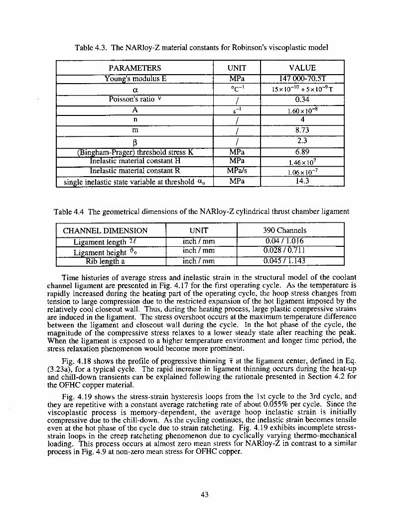
Table4.3. TheNARloy-Z materialconstantsfor Robinson'sviscoplasticmodel
PARAMETERS
Young'smodulusE
Poisson'sratio vA
m
(Bingham-Prager) threshold stress KInelastic material constant H
UNIT
MPa
oc-1
-Is
MPa
MPa
VALUE
147 000-70.5T
15x10 -10 + 5x 10--gT
0.34
1.60 x 10 -8
4
8.73
2.3
6.89
1.46 x 10⁷
Inelastic material constant R MPa/s 1.06 x 10 .7
single inelastic state variable at threshold So MPa 14.3
Table 4.4 The geometrical dimensions of the NARloy-Z cylindrical thrust chamber ligament
CHANNEL DIMENSION
Ligament length 2g
Ligament height OoRib length a
UNIT
inch / mm
inch / mm
inch / mm
390 Channels
0.04 / 1.016
0.028 / 0.711
0.045 / 1.143
Time histories of average stress and inelastic strain in the structural model of the coolantchannel ligament are presented in Fig. 4.17 for the first operating cycle. As the temperature israpidly increased during the heating part of the operating cycle, the hoop stress changes fromtension to large compression due to the restricted expansion of the hot ligament imposed by therelatively cool closeout wall. Thus, during the heating process, large plastic compressive strainsare induced in the ligament. The stress overshoot occurs at the maximum temperature differencebetween the ligament and closeout wall during the cycle. In the hot phase of the cycle, themagnitude of the compressive stress relaxes to a lower steady state after reaching the peak.When the ligament is exposed to a higher temperature environment and longer time period, thestress relaxation phenomenon would become more prominent.
Fig. 4.18 shows the profile of progressive thinning _ at the ligament center, defined in Eq.(3.23a), for a typical cycle. The rapid increase in ligament thinning occurs during the heat-upand chill-down transients can be explained following the rationale presented in Section 4.2 forthe OFHC copper material.
Fig. 4.19 shows the stress-strain hysteresis loops from the 1st cycle to the 3rd cycle, andthey are repetitive with a constant average ratcheting rate of about 0.055% per cycle. Since theviscoplastic process is memory-dependent, the average hoop inelastic strain is initiallycompressive due to the chill-down. As the cycling continues, the inelastic strain becomes tensileeven at the hot phase of the cycle due to strain ratcheting. Fig. 4.19 exhibits incomplete stress-strain loops in the creep ratcheting phenomenon due to cyclically varying thermo-mechanicalloading. This process occurs at almost zero mean stress for NARIoy-Z in contrast to a similarprocess in Fig. 4.9 at non-zero mean stress for OFHC copper.
43
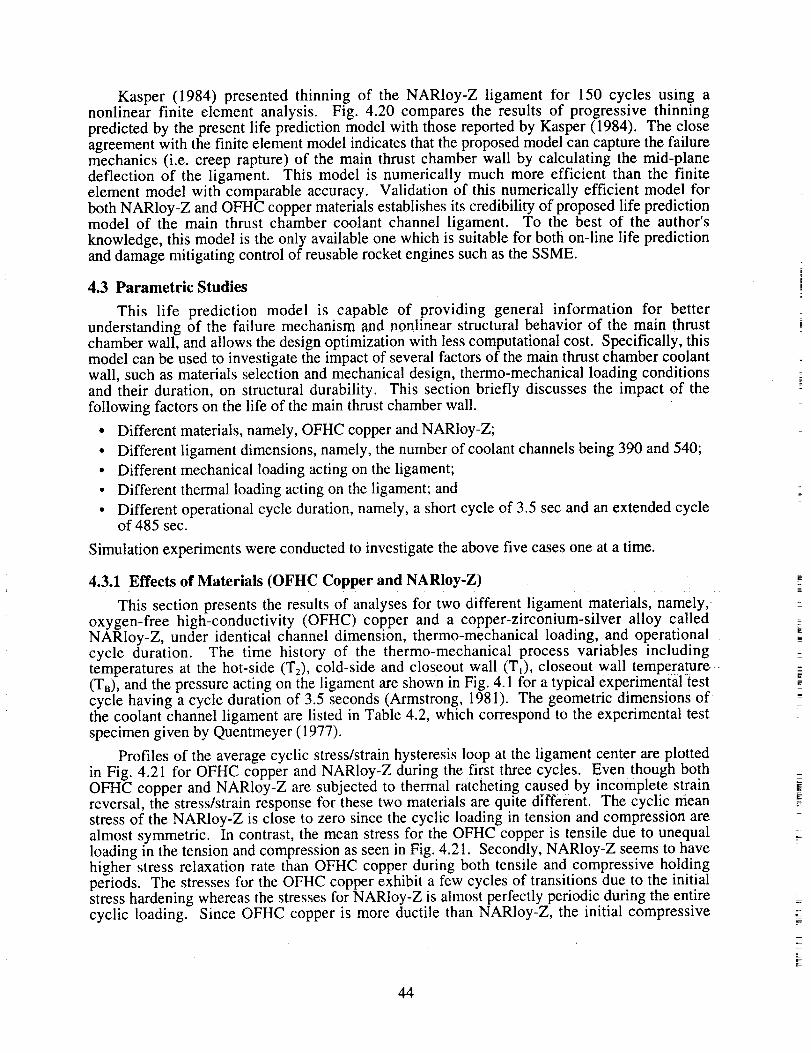
Kasper (1984) presentedthinning of the NARloy-Z ligament for 150 cycles using anonlinear finite element analysis. Fig. 4.20 comparesthe results of progressivethinningpredictedby thepresentlife predictionmodelwith thosereportedby Kasper(1984). The closeagreementwith thefinite elementmodelindicatesthattheproposedmodelcancapturethefailuremechanics(i.e. creeprapture) of the main thrust chamberwall by calculating the mid-planedeflection of the ligament. This model is numerically much more efficient than the finiteelementmodel with comparableaccuracy. Validation of this numericallyefficient model forbothNARIoy-Z andOFHCcoppermaterialsestablishesits credibility of proposedlife predictionmodel of the main thrust chambercoolant channel ligament. To the best of the author'sknowledge,thismodel is theonly availableonewhich is suitablefor bothon-line life predictionanddamagemitigatingcontrolof reusablerocketenginessuchastheSSME.
4.3 Parametric Studies
This life prediction model is capable of providing general information for betterunderstanding of the failure mechanism and nonlinear structural behavior of the main thrustchamber wall, and allows the design optimization with less computational cost. Specifically, this
model can be used to investigate the impact of several factors of the main thrust chamber coolantwall, such as materials selection and mechanical design, thermo-mechanical loading conditionsand their duration, on structural durability. This section briefly discusses the impact of the
following factors on the life of the main thrust chamber wall.
• Different materials, namely, OFHC copper and NARloy-Z;
• Different ligament dimensions, namely, the number of coolant channels being 390 and 540;
° Different mechanical loading acting on the ligament;
• Different thermal loading acting on the ligament; and
• Different operational cycle duration, namely, a short cycle of 3.5 sec and an extended cycleof 485 sec.
Simulation experiments were conducted to investigate the above five cases one at a time.
4.3.1 Effects of Materials (OFHC Copper and NARloy-Z)
This section presents the results of analyses for two different ligament materials, namely,oxygen-free high-conductivity (OFHC) copper and a copper-zirconium-silver alloy calledNARIoy-Z, under identical channel dimension, thermo-mechanical loading, and operationalcycle duration. The time history of the thermo-mechanical process variables includingtemperatures at the hot-side (T2), cold-side and closeout wall (T_), closeout wall temperature(TB), and the pressure acting on the ligament are shown in Fig. 4.1 for a typical experimental test
cycle having a cycle duration of 3.5 seconds (Armstrong, 1981). The geometric dimensions ofthe coolant channel ligament are listed in Table 4.2, which correspond to the experimental test
specimen given by Quentmeyer (1977).
Profiles of the average cyclic stress/strain hysteresis loop at the ligament center are plottedin Fig. 4.21 for OFHC copper and NARloy-Z during the first three cycles. Even though bothOFHC copper and NARloy-Z are subjected to thermal ratcheting caused by incomplete strainreversal, the stress/strain response for these two materials are quite different. The cyclic mean
stress of the NARIoy-Z is close to zero since the cyclic loading in tension and compression arealmost symmetric. In contrast, the mean stress for the OFHC copper is tensile due to unequalloading in the tension and compression as seen in Fig. 4.21. Secondly, NARIoy-Z seems to havehigher stress relaxation rate than OFHC copper during both tensile and compressive holdingperiods. The stresses for the OFHC copper exhibit a few cycles of transitions due to the initialstress hardening whereas the stresses for NARIoy-Z is almost perfectly periodic during the entirecyclic loading. Since OFHC copper is more ductile than NARloy-Z, the initial compressive
-=
m
44
plastic strain of OFHC copper is more pronounced than that of NARloy-Z. The creep ratchetingis about 0.06% per cycle for OFHC copper and about 0.055% per cycle for NARIoy-Z.
Once substantial bulging occurs, the thermal and structural characteristics in the vicinity ofthe bulging region changes because of the deformation in geometry. Since this deformation ofthe ligament is updated at each instant of time in the life prediction model, the resulting effectson creep ratcheting are more severe for the OFHC copper than those for NARIoy-Z.Consequently, OFHC copper suffers from a larger bulging-out as shown in Fig. 4.22. The plasticflow and bulging-out of the inner wall for NARIoy-Z are smaller than those for OFHC copper.This prediction is consistent with the damage observed in actual test chambers as reported byHannum et al. (1976). The thinning of OFHC copper ligament is about ten times larger than thatof the NARloy-Z chamber as seen in Fig. 4.22. Both simolation results and experimentalobservations demonstrate that NARIoy-Z materials show an improvement in cyclic life over theOFHC copper under the identical thermo-mechanical loading.
4.3.2 Effects of Ligament Dimensions (Number of 390 and 540 Channels)
This section presents the results of analyses for different number of coolant channels underidentical thermo-mechanical cyclic loading and duration for both OFHC copper and NARloy-Z.The time histories of the chamber wall temperatures and pressure are displayed in Fig. 4.1.Geometric dimensions for different configurations of the coolant channel are listed in Table 4.5.
Table 4.5 Different geometrical configurations for the main thrust chamber ligament
CHANNEL DIMENSION Unit 390 Channels 540 Channels
inch / mm 0.04 / 1.016 0.029 / 0.7338Ligament length 2g
Ligament height Oo
Rib length a
inch / mm
inch / mm
0.028 / 0.711
0.045 / 1.143
0.028 / 0.711
0.0325 / 0.8255
Profiles of the average cyclic stress/strain hysteresis loops at ligament center are plotted inFigs. 4.23 and 4.24 for OFHC copper and NARIoy-Z, respectively, for the first three cycles. Fig.4.23 shows almost identical stress and plastic strain for different ligament dimensions forNARloy-Z material under identical thermo-mechanical loading. In contrast, the average plasticstrains of OFHC copper ligament, as seen in Fig. 4.23, are different for the two different ligamentdimensions. The rationale is that OFHC copper is more ductile than NARloy-Z and therebysuffers from larger inelastic deformation which, in turn, influences the structural model by thegeometric updating process.
Figs. 4.25 and 4.26 show the normalized thinning, _, of the ligament for both OFHC copperand NARloy-Z materials, respectively, for the two different ligament configurations. For OFHC
copper, _ is about ten times larger than that of NARIoy-Z due to the different materialcharacteristics as discussed in Section 4.4.1. If the ratio of the length to height is made larger asseen in Table 4.5 for 390 channels, the ligament becomes more flexible resulting in increasedbulging-out. Therefore, for both materials, thinning of the ligament with 390 channels is morepronounced than that with 540 channels as seen in Figs. 4.25 and 4.26. In other words, themechanical design with 540 channels will yield a longer service life of the main thrust chamberthan that for 390 channels under identical thermo-mechanical loading.
4.3.3 Effects of Mechanical Loading
Since the main thrust chamber coolant wails are subjected to severe cyclic loading ofpressure and temperature, the resulting stresses and plastic strains cause incremental bulging out.To assess the role that pressure loading plays on the so-called doghouse effect (Hannum et al.,1976), the coolant ligament was analyzed for different pressure (mechanical) loading under
45

identical ligamentconfiguration,temperature(thermal)loading,andoperationalcycleduration.The time historyof themechanicalloading,namely,pressuredifferenceactingon theligament,AP(t) = [P1(t)- P2(t)], is shownin Fig. 4.27wherethemagnitudeof pressuredifferenceactingon theligament, AP, is increasedtwofold. Thetemperatureloadinghistory is shownin Fig. 4.1for OFHCcopperandtheligamentdimensionsarelistedin Table 4.2.
Creep ratcheting which is largely induced by the pressure difference is discussed byPorowski et al., (1985). Bending stresses due to the cyclic pressure loading cause a plastic
deformation and bulging-out of the ligament during each firing cycle. The time history of theaverage stress/strain hysteresis loop at the ligament center are plotted in Figs. 4.28 and Fig. 4.29for OFHC copper and NARloy-Z ligaments during the first three cycles. As the pressuredifference is increased twofold, plastic strain and creep ratcheting rate per cycle for OFHC
copper change much more significantly than those for NARIoy-Z which is less ductile material.
Normalized thinning of the ligament for twofold increase in pressure loading is shown in
Figs. 4.30 and 4.31 for OFHC copper and NARloy-Z, respectively. The thinning rate isincreased about two times for both OFHC copper and NARloy-Z. The resulting "doghouse"
effect predicted here is a result of pressure difference across the coolant channel wall which isalso observed in the experiments (Hannum et al., 1976)
4.3.4 Effects of Thermal Loading
Hannum et al (1976) and Quentmeyer (1977) reported that the cycles to failure could becorrelated with either hot-side wall temperature, or the difference between hot-side wall andcloseout wall temperatures. In order to determine the effects of different temperature (thermal)loading on the thrust chamber life, the following four sets of different temperature loading as
depicted in Figs. 4.32 and 4.33 were investigated under identical pressure loading, ligamentdimension, and operational cycle. The time history of the pressure (mechanical) loading isshown in Fig. 4. lb and the geometric dimension is listed in Table 4.2. For each of the following
four cases, the closeout wall temperature, T 8 , was kept unchanged.
• Case A in Fig. 4.32a serving as the baseline case in which the superscript * indicates the
reference profile for the hot-side wall temperature, T2, and the cold-side wall temperature,Ti.
• Case B in Fig. 4.32b representing a increased average wall temperature situation where T2:,g
is increased by about 150°K over T 2 during the hot phase of the firing cycle, and T_ is
kept equal to T 1 .
• Case C in Fig. 4.33a representing a increased average wall temperature situation with no
temperature difference across the ligament where T_ is increased to T 2 during the hot
phase of the firing cycle, and T2 is kept equal to T 2
• Case D in Fig. 4.33b representing a decreased average wall temperature situation where8t
Tj decreased by about 150°K from T I during the hot phase of the firing cycle, and T2 is
kept equal to T 2.
Figs 4.34 and 4.35 plot the stress/strain hysteresis loops for OFHC copper and NARIoy-Z,respectively, under four different temperature loading. For Case D, which is the only case wherethe average ligament temperature is decreased during the hot phase of the firing cycle, themagnitude of both tensile and compressive stresses are reduced and the initial plastic strain isless compressive. This observation is more pronounced for OFHC copper as seen in Fig. 4.34due to its ductility. The plastic strain range in the ligament is largely dependent on the thermalstrain range which is a function of the transient difference between the average ligament
46
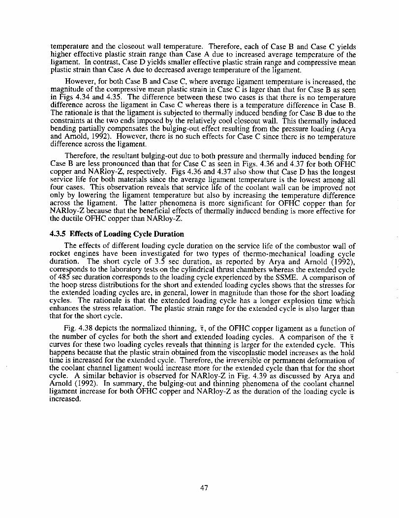
temperatureand thecloseoutwall temperature.Therefore,eachof CaseB andCaseC yieldshigher effective plastic strain rangethanCaseA due to increasedaveragetemperatureof theligament. In contrast,CaseD yieldssmallereffectiveplasticstrainrangeandcompressivemeanplasticstrainthanCaseA dueto decreasedaveragetemperatureof theligament.
However,for bothCaseB andCaseC, whereaverageligamenttemperatureis increased,themagnitudeof thecompressivemeanplasticstrainin CaseC is lagerthan thatfor CaseB asseenin Figs 4.34 and4.35. Thedifferencebetweenthesetwo casesis that thereis no temperaturedifferenceacrossthe ligament in CaseC whereasthereis a temperaturedifferencein CaseB.Therationaleis thatthe ligamentis subjectedto thermallyinducedbendingfor CaseB dueto theconstraintsat thetwo endsimposedby therelativelycool closeoutwall. This thermally inducedbendingpartially compensatesthebulging-outeffect resultingfrom the pressureloading (AryaandArnold, 1992). However,thereis no sucheffects for CaseC sincethereis no temperaturedifferenceacrosstheligament.
Therefore,theresultantbulging-outdueto bothpressureandthermally inducedbendingforCaseB arelesspronouncedthanthat for CaseC asseenin Figs.4.36 and4.37 for bothOFHCcopperandNARIoy-Z, respectively.Figs4.36and4.37alsoshowthat CaseD hasthe longestservicelife for both materialssincethe averageligament temperatureis the lowest amongallfour cases. This observationrevealsthat servicelife of the coolantwall canbe improvednotonly by lowering the ligament temperaturebut also by increasingthe temperaturedifferenceacrossthe ligament. The latter phenomenais more significant for OFHC copper than forNARloy-Z becausethatthebeneficialeffectsof thermallyinducedbendingis moreeffectivefortheductileOFHCcopperthanNARloy-Z.
4.3.5 Effects of Loading Cycle Duration
The effects of different loading cycle duration on the service life of the combustor wall ofrocket engines have been investigated for two types of thermo-mechanical loading cycleduration. The short cycle of 3.5 sec duration, as reported by Arya and Arnold (1992),
corresponds to the laboratory tests on the cylindrical thrust chambers whereas the extended cycleof 485 sec duration corresponds to the loading cycle experienced by the SSME. A comparison ofthe hoop stress distributions for the short and extended loading cycles shows that the stresses forthe extended loading cycles are, in general, lower in magnitude than those for the short loadingcycles. The rationale is that the extended loading cycle has a longer explosion time whichenhances the stress relaxation. The plastic strain range for the extended cycle is also larger thanthat for the short cycle.
Fig. 4.38 depicts the normalized thinning, _, of the OFHC copper ligament as a function of
the number of cycles for both the short and extended loading cycles. A comparison of the
curves for these two loading cycles reveals that thinning is larger for the extended cycle. Thishappens because that the plastic strain obtained from the viscoplastic model increases as the holdtime is increased for the extended cycle. Therefore, the irreversible or permanent deformation ofthe coolant channel ligament would increase more for the extended cycle than that for the shortcycle. A similar behavior is observed for NARioy-Z in Fig. 4.39 as discussed by Arya andArnold (1992). In summary, the bulging-out and thinning phenomena of the coolant channelligament increase for both OFHC copper and NARloy-Z as the duration of the loading cycle isincreased.
47
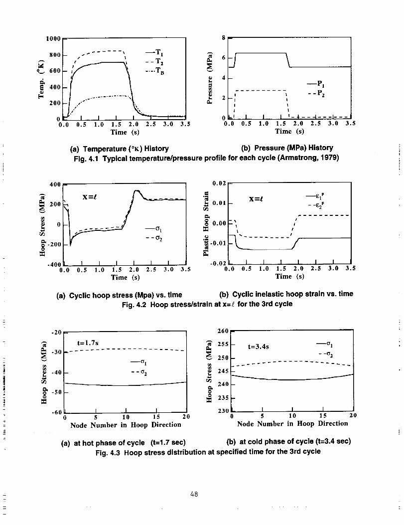
1000 -
800 -
600
400
200
00.0
8 D
...... T 1
_ _ T2
.... TB
is.S t.-"'- •s oS "_
I 1 I I I I'0.5 1.0 1.5 2.0 2.5 3.0 3.5
Time (s)
_JI,d
¢/}
t.
¢h
6J4-
I
2 --II
!
0 bJ0.0
\
I0.5
L - - P2!
t
I
1 I t- -I. - - -t- - -I- - -1.0 1.5 2.0 2.5 3.0 3.5
Time (s)
(a) Temperature (°K) History (b) Pressure (MPa) History
Fig. 4.1 Typical temperature/pressure profile for each cycle (Armstrong, 1979)
400 -
200
_ or_
"-20o
¢
-400
__ - -G 2
¢,m
r_
0.02 -
0.01X-'_ --EIP
-- _ -F_.2 p
I
0.00 - _
I I
-0.01m
0.5I I I I I I I -0.02 I I I I I
0.5 1.0 1.5 2.0 2.5 3.0 3.5 0.0 1.0 1.5 2.0 2.5 3.0 3.5
Time (s) Time (s)
(a) Cyclic hoop stress (Mpa) vs. time (b) Cyclic Inelastic hoop strain vs. time
Fig. 4.2 Hoop stress/strain at x=_ for the 3rd cycle
L.
-20 -
-30
-40
-50
-60 10
t=l.7s
--O 1
_ - - 02
260
255
250
_ 24st.
240
g235
- t=3.4s _°1
- -O 2
I [ I 230 I I 15 l0 15 20 0 5 10 15
Node Number in Hoop Direction Node Number in Hoop Direction
20
(a) at hot phase of cycle (t=1.7 sec) (b) at cold phase of cycle (t=3.4 sec)
Fig. 4.3 Hoop stress distribution at specified time for the 3rd cycle
48
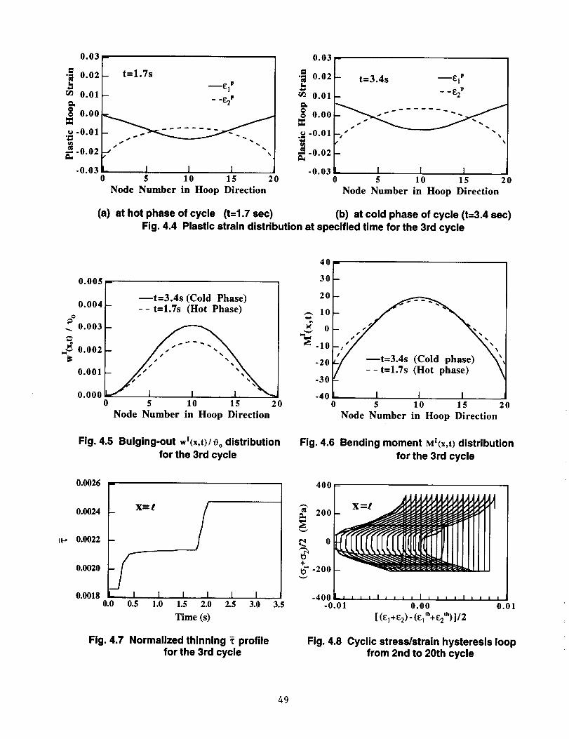
0.03
•_ 0.02
0.01
0.00
-0.01
_ -0.02
-0.030
m
_ t=l.7s
_EI p
m - __2p
I I I5 10 15 20
Node Number in Hoop Direction
0.03
•_ 0.02- t=3.4s mEIP
--_2"r_ 0.01
I 0.00 i" " " " "-0.01 "
-0.02 _-.0.03 _ I I I
0 5 10 15 20
Node Number in Hoop Direction
(a) st hot phase of cycle (t=1.7 sec) (b) at cold phase of cycle (t=3.4 sec)
Fig. 4.4 Plastic strain distribution at specified time for the 3rd cycle
0.005 -
0.004
O
0.003
._,_ 0.002
0.001
0.000
mt=3.4s (Cold Phase)
-- t=l.7s (Hot Phase)
0 5 10 15 20
Node Number in Hoop Direction
Fig. 4.5 Bulging-out wI(x,t)/Oo distributionfor the 3rd cycle
40-
30
20
10
0
-10
-20
-30
-40
/ mt=3.4s (Cold phase) _
-- t=l.7s (Hot phase) _J/
_ I I I I
0 5 10 15 20
Node Number in Hoop Direction
Fig. 4.6 Bending moment Ml(x,t) distributionfor the 3rd cycle
|P
0.0026
0.0024
0.0022
0.0020
0.0018
x=, /m
J--L I I I 1
0.0 0.5 1.0 1.5 2.0
Time (s)
I I2.5 3.0
Fig. 4.7 Normalized thinning _ profilefor the 3rd cycle
400[-
.400 L' ' i i I i ' ' ' I , _ , , I , , , ,3.5 -0.01 0.00 0.01
[ (_1+ _) - (El'h+ _ 'h) ]/2
Fig. 4.8 Cyclic stress/strain hysteresis loopfrom 2nd to 20th cycle
49
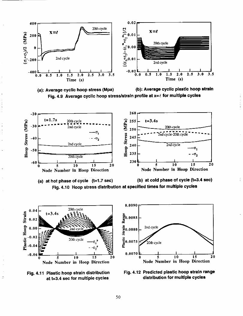
400 -
200
_ 0
+
--2oo
__ X--.._/_X=l _ 20th_cycle X=t
20th cycle
2nd cycle
I I I I I I I I I I I
0.5 1.0 1.5 2.0 2.5 3.0 3.5 0.5 1.0 1.5 2.0 2.5 3.0 3.5
Time (s) Time (s)
(a): Average cyclic hoop stress (Mpa) (b): Average cyclic plastic hoop strain
Fig. 4.9 Average cyclic hoop stress/strain profile at x= _ for multiple cycles
-20 -
-40
-50o
-60
m
t= 1.7s 20th cycleme m w am az Im m Im m ll II II II ll I Im I lm n m m mS m
2nd cycle
• _ -(i 2
2nd cycle
20th cycle
I I I0 5 10 15 20
Node Number in Hoop Direction
260
25525O
245
24OeLoo
235
230
- t=3.4s
20th cycle
....... "2n 'cyc 3o' 'cycr .......
_ 2nd cycle
I I I
0 5 10 15 20
Node Number in Hoop Direction
(a) at hot phase of cycle (t=1.7 sec) (b) at cold phase of cycle (t=3.4 sec)
Fig. 4.10 Hoop stress distribution at specified times for multiple cycles
0.04
0.02
0.00
-0.02
-0.04
-0.06
t=3.4s20th cycle
20th cycle _£1p
- -_2 p
I 10 5 10 15 20
Node Number in Hoop Direction
Fig. 4.11 Plastic hoop strain distributionat t=3.4 sec for multiple cycles
0"0090 I_0.0085
0.0080
"_0.0075
0.0070I I t
0 5 10 15 20
Node Number in Hoop Direction
Fig. 4.12 Predicted plastic hoop strain rangedistribution for multiple cycles
50
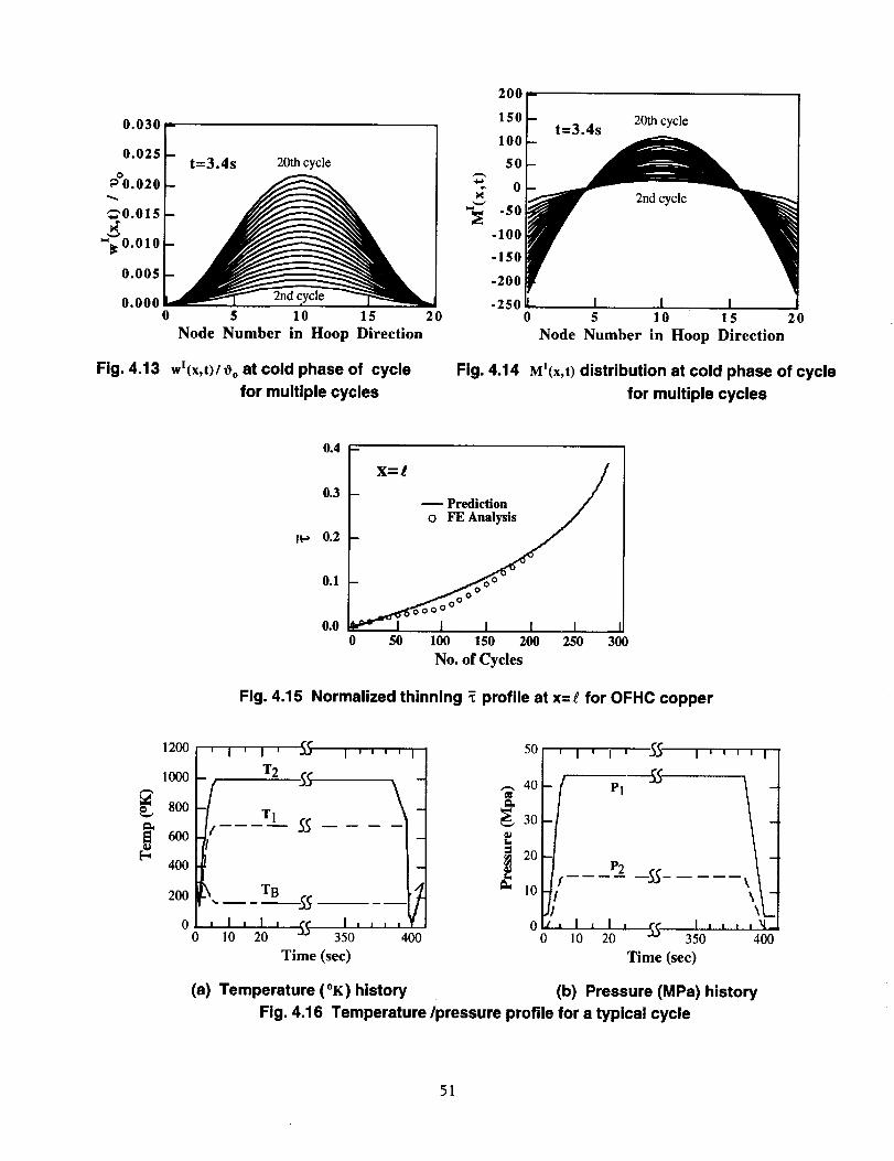
0.030 -/
0.025 _ t=3.4s 20thcycle
0.020
0.015
"_: 0.010
0.005
0.000 i_0 5 10 15 20
Node Number in Hoop Direction
Fig. 4.13 wl(x,t)/Oo at cold phase of cycle
for multiple cycles
200
150 F
100
50
-50
-100
-150
-200
-2500
t=3.4s 20th cycle
2nd cycle
I I5 10 15
Node Number in Hoop Direction
20
Fig. 4.14 Ml(x,t) distribution at cold phase of cycle
for multiple cycles
0.4
0.3
Iv 0.2
0.1
0.0
X=/ /- -- Prediction
_ o FE Analysis/
__o I I
O o
O ooOO O
I0 50 100 150 200 250 300
No. of Cycles
Fig. 4.15 Normalized thinning _ profile at x=_ for OFHC copper
1200
1000
ro 8OO
6o0
200
00
T2
TI
TB
5O
"_ I ' I ' ' It
SS \-
55
._ I , , , ,350 400
Time (sec)
_-, 40
eL
___ 30
10
' I ' I ' -_
( el
I,i_ I
P2
\
I I I , 0 I , I , I I 55 I , I , I'l-l 0 20 0 10 20 350 400
Time (sec)
(a) Temperature (°K) history (b) Pressure (MPa) history
Fig. 4.16 Temperature/pressure profile for a typical cycle
51
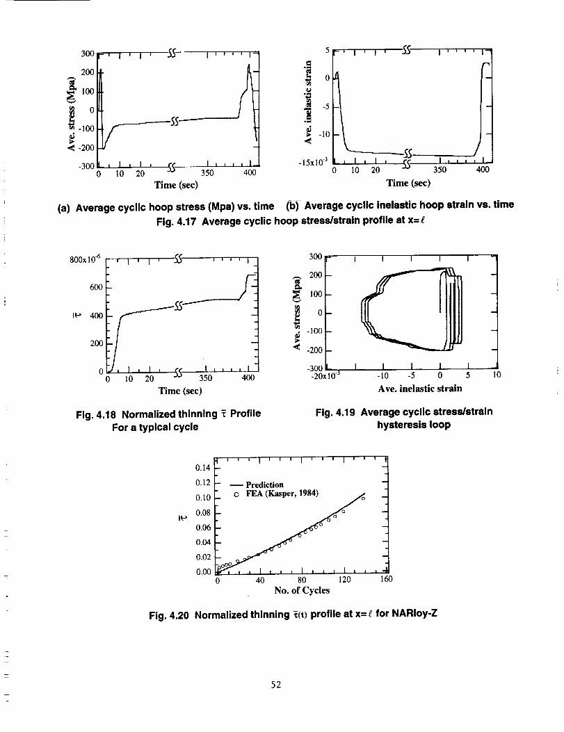
300 r' I ' I ' 55 I ' ' ' 5
100 '_¢_
o -5
_10
•_ -200_300 L , ! k I ,........(e I t ,..,., I1 -15x10 30 10 20 "" 350 400 0 10 20 350 400
Time (see) Time (see)
(a) Average cyclic hoop stress (Mpa) vs. time (b) Average cyclic inelastic hoop strain vs. time
Fig. 4.17 Average cyclic hoop stress/strain profile at x=g
800x10"6 +_ I ' I ' -_ ' ' ' ' ;t 300
0 I , , , l..I0 I0 20 350 400
600
IP 400
Time (sec)
Fig. 4.18 Normalized thinning _ Profile
For a typical cycle
2_ -
•-1_ -
-2_ -
-300 - , I-20x10-"
Fig. 4.19
I I
i I 1-I0 -5 0
I
Ave. inelastic strain
Average cyclic stress/strain
hysteresis loop
m
I0
0.14
0.12
0.10
it-" 0.08
0.06
0.04
0.02
0.00
_ ' ' ' I ' ' ' I ' ' ' I ' ' ' ._-1-- Prediction
- oCO
"°_i_l , l , , , i l i l l , , ,.j
0 40 80 120 160
No. of Cycles
Fig. 4.20 Normalized thinning i(t) profile at x= t' for NARIoy-Z
52
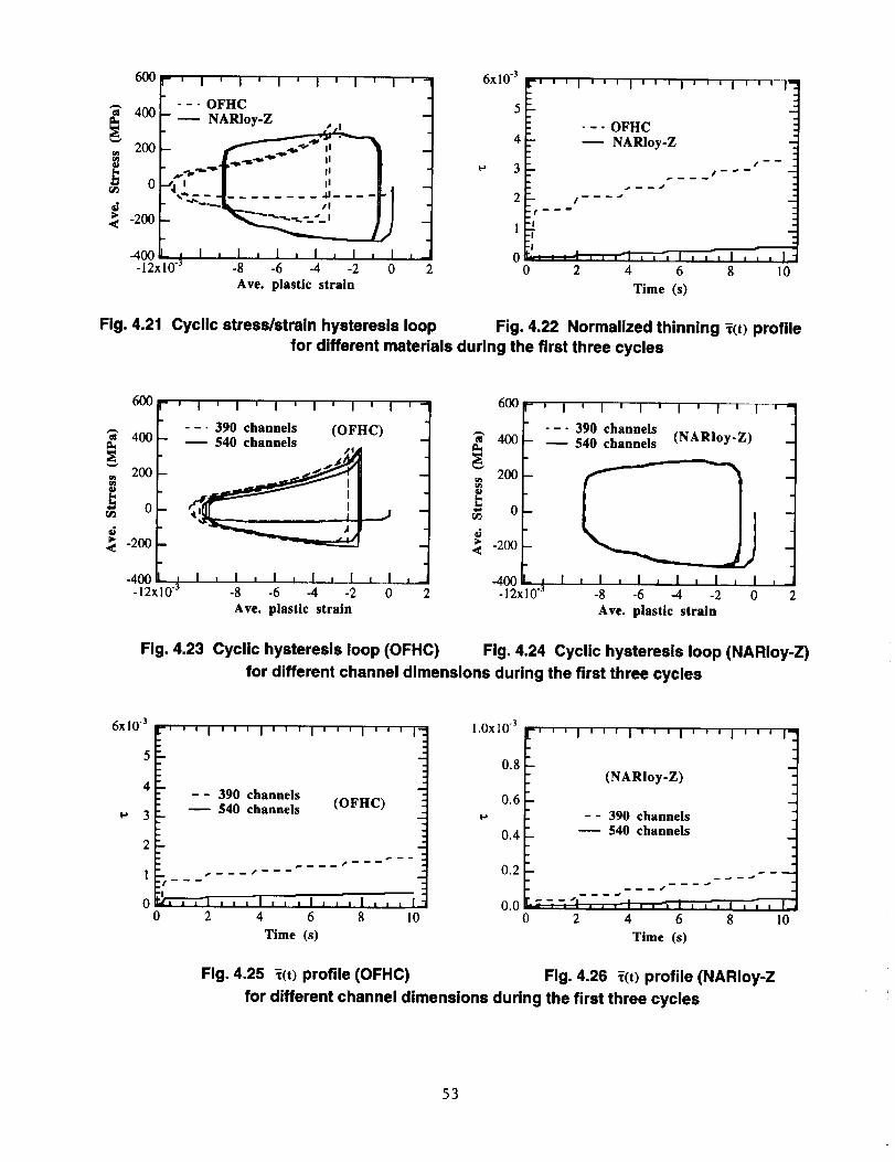
600p.- , i , i , i ; i ; i , i ,I.-
] - -- oFI-I_
400F _ NARioy-Z • i
200I-L IIr
I/", I ,'
1 ........ .... !.._=. _
-400 L , I , I , I , I , I ,-12x10 -3 -8 -6 -4 -2 0
Ave. plastic strain
J2
6xlO -3 I_I '' I ''' I I ' ' I' '' I I I ' l_
--- OFHC
4 -- NARloy-Z
3 /--_--/----
2 i ---J
"¢_---
1"2-!
0 "! ' ' ' ' I ' I , i i I--
0 2 4 6 8 10
Time (s)
Fig. 4,21 Cyclic stress/strain hysteresis loop Fig. 4.22 Normalized thinning _(t) profilefor different materials during the first three cycles
600
400
200
0
-200
r ' i , i , i I I ' I ' I ' -
" --- 390 channels (OFHC)
540 channels /_
-400- ' I , I I I t I , I , I ,.2-12X10 3 -8 -6 -4 -2 0 2
Ave. plastic strain
6_
2_
_ o
_ -2_
-4__12x10 "3
I- ' I ' I ' I ' I I I ' I ' -
" --- 390 channels540 channels (NARIoy-Z)
-ljL , I , I , I , I , I , I , /
-8 -6 -4 -2 0 2
Ave. plastic strain
Fig. 4.23 Cyclic hysteresis loop (OFHC) Fig. 4.24 Cyclic hysteresis loop (NARIoy-Z)
for different channel dimensions during the first three cycles
6x10³ 7' ' ' I , , i I ' ' i I ' ' ' I I , , I:
5
4
*-" 3
2
. =
-- 390 channels540 channels (OFHC)
_ I I I / _ I I _ I I
O_ , i l I , , , I , , ,1 ,, , i-0 2 4 6 8 I0
Time (s)
l.OxlO 3
0.8
0.6
ta
0.4
0.2
0.0
(NARloy-Z)
-- 390 channels540 channels
0 2 4 6 8
Time (s)
I0
Fig. 4.25 _(t) profile (OFHC) Fig. 4.26 _(t) profile (NARIoy-Z
for different channel dimensions during the first three cycles
53
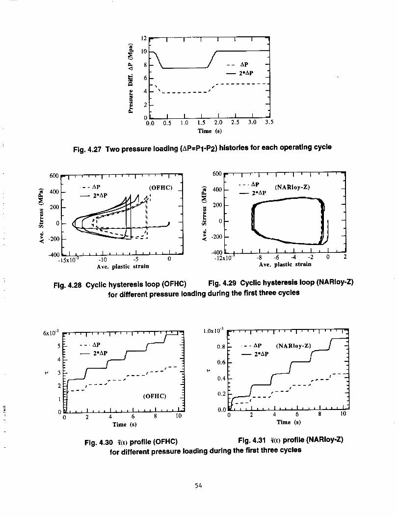
12
6-4 " ""
o_- i0.0 0.5
I I I I I I
-- Ap
-- 2*AP
I I I1.0 1.5 2.0
Time (s)
I I -
2.5 3.0 3.5
Fig. 4.27 Two pressure loading (AP=P1-P2) histories for each operating cycle
_" 400
_ 0
_ -200
600'-I ' ' ' ' I ' ' ' ' I [r l ' ' I '
- - AP (OFHC)
-400_ 15x 10 .3 - i 0 -5 0
Ave. plastic strain
600 - , I ' I _ I _ I ' I ' 1 '
. -. Ap (NARIoy-Z)400 -- 2*AP
200
o-
L.,_ -200
400 , I , I , I , I _ I , I , --12x10 3 -8 -6 -4 -2 0 2
Ave. plastic strain
Fig. 4.28 Cyclic hysteresis loop (OFHC) Fig. 4.29 Cyclic hysteresis loop (NARIoy-Z)
for different pressure loading during the first three cycles
6x10 -3
5
4
3
-, , , I , _ , I ' _ ' I _ '_d-J- -. AP
=
I
(OFHC)
t ,,I ,,, I,_ _1, ,,I ,,, I-0 2 4 6 8 10
Time (s)
l.OxlO "3
0.8
0.6
0.4
0.2
0.00
-' ' 'I _'' I °' 'I' ''I ''' I'
,- - AP (NARloy-Z)
-- 2*AP S "
I
t
,,, I,,, I,, ,1, , ,I ,,, i_2 4 6 8 10
Time (s)
Fig. 4.30 ](t) profile (OFHC) Fig. 4.31 i(t) profile (NARIoy-Z)
for different pressure loading during the first three cycles
54
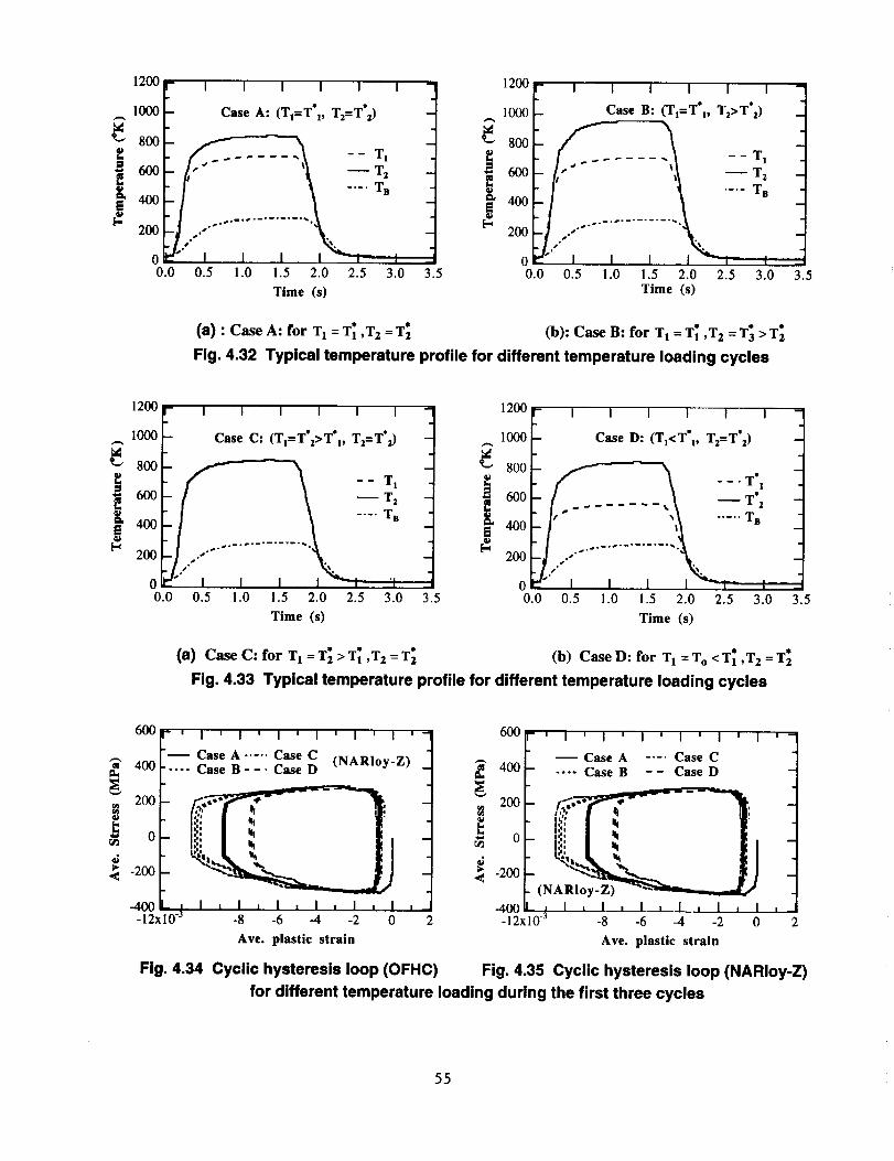
1200
1000
soo
•P- 600
4oo200
- I I I I I I -- o
Case A: (TI=T" p T2=T*2)
T,
_ T2 -
.... T B -
i I "0.0 0.5 1.0 1.5 2.0 2.5 3.0 3.5
Time (s)
1200
1000
800
600
400i
200
- I I I I I I -
Case B: (TI=T" . T.>T'z)
/," ',1 -- T2 -
0.0 0.5 1.0 1.5 2.0 2.5 3.0 3.5Time (s)
(a) : Case A: for T 1 = T1 ,T 2 = T2 (lo): Case B: for T1 = T 1 ,T 2 = T; > T_
Fig. 4.32 Typical temperature profile for different temperature loading cycles
1200 _-- I I I I I I ] 1200 _ I I I I I I -/ 1 1-
1000 Case C: (T1=T*z>T'I, T2=T' z) 1000 _- Case D: (TI<T" . T2=T*2) -
__ T1 ---T ! .600 _ T2 600 ........ _ T"2 -
400 400 _/" ............... _l._ ..... TB -
0.0 0.5 1.0 1.5 2.0 2.5 3.0 3.5 0.0 0.5 1.0 1.5 2.0 2.5 3.0 3.5
Time (s) Time (s)
(S) Case C: for T 1 = T_ > T 1 ,T 2 = T_ (b) Case D: for T1 = TO < T1 ,T 2 = T_
Fig. 4.33 Typical temperature profile for different temperature loading cycles
600
_" 400
,_ 200
,_ -200
" ' I ' I ' I ' I ' I ' I '
"-- Case A ..... Case C ............ Case B--. Case D trqAKIoY'l")
t ._ w
IX, I _ I,,,,¢|1i|!
"¢1
- 600
200
o
_ -200
-400- ' I , I , I , I , I . I ,-12x10 "3 -8 -6 -4 -2 0 2
Ave. plastic strain
Fig. 4.34 Cyclic hysteresis loop (OFHC)
- ' I ' I ' I ' I ' I ' I ' _
• _ Case A .... Case C- ---- CaseB -- CaseD
• I;;': _ - - .... , "
I',': l ,_ i" qi! n i I
- (NARIoy-Z) -_--_itm.....,.._g/-400 L i I l I n I I I , I , I , I-12xl0 3 -8 -6 -4 -2 0 2
Ave. plastic strain
Fig. 4.35 Cyclic hysteresis loop (NARIoy-Z)
for different temperature loading during the first three cycles
55
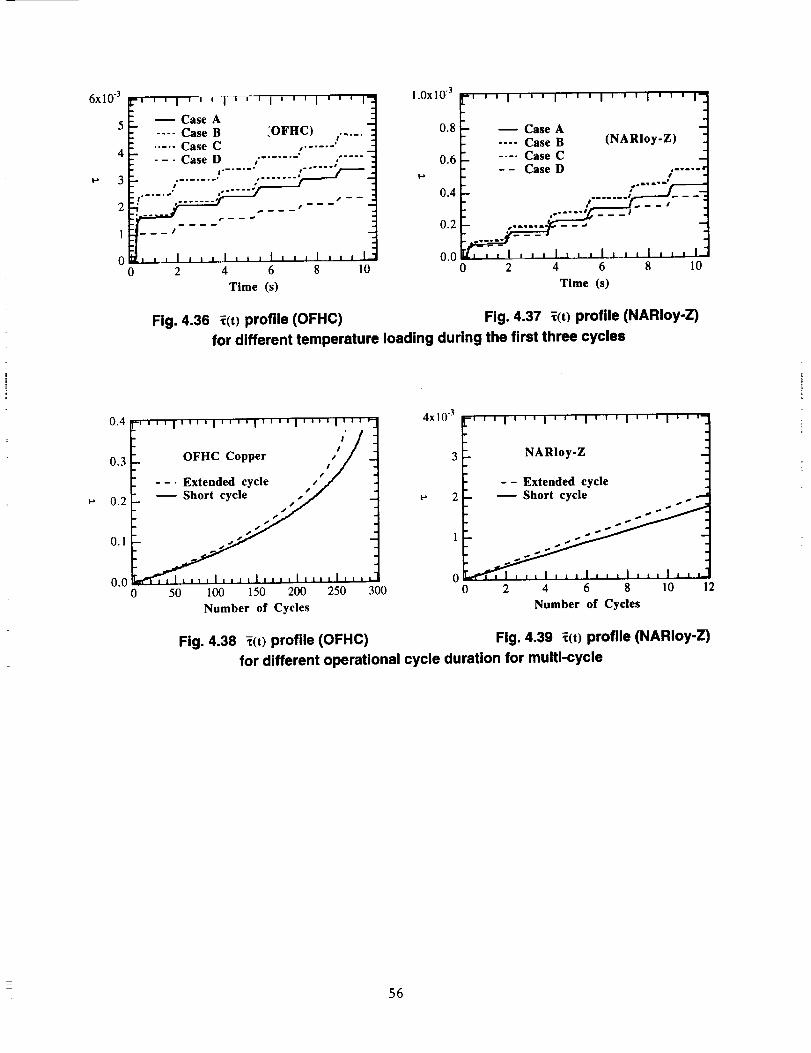
6xl0 -3
5
4
3
2
1
i , , i , , , i , , _ I , , , I , , , I_]
Case A _1.... Case B _OFHC) ,..... |
..... Case C " ..... ' -I
---CaseD '........ _ : ..... "l
........:.......•.......
0 2 4 6 8 10
Time (s)
1.0xl0 3
0.8
0.6
0.4
0.2
0.0
"''' I''' I''' I''' I''' I_
.... Case (NARIoy-
.... Case c-- Case D .....
0 2 4 6 8 10
Time (s)
Fig. 4.36 _(t) profile (OFHC) Fig. 4.37 _(t) profile (NARIoy-Z)
for different temperature loading during the first three cycles
0.4
0.3
0.2
0.1
0.0
-,,,,1''''1''''1''''1''''1'''"
OFHC Copper t,,ty (
--. Extended cycle r t._
Short cycle/
_[, , _ _ I l ,, , I i , _
0 50 100 150 200 250
Number of Cycles
4x10 -3
_' 2
1
• 0300
-, , , i , ,, i , , , i , , , i , ,, I , , ,
NARIoy-Z
-- Extended cycleShort cycle ...-
0 2 4 6 8 10 12
Number of Cycles
Fig. 4.38 i(t) profile (OFHC) Fig. 4.39 _(t) profile (NARIoy-Z)
for different operational cycle duration for multi-cycle
56

CHAPTER 5
INTEGRATED LIFE EXTENSION AND CONTROL OF THE REUSABLE ROCKET ENGINE
The general structure of the damage mitigating control system is briefly described in Section1.3.4 of Chapter 1. The major tasks in the synthesis of the damage mitigating control system inFig. 5.1 are:
(i) Formulation of an appropriate dynamic model of the plant (e.g., the Space Shuttle MainEngine);
(ii) Formulation of the structural model and damage model of the critical plant components(e.g., turbine blades and main thrust chamber coolant channel ligament);
(iii) Synthesis of a feedforward control policy with the objective of achieving structuraldurability and high performance; and
(iv) Synthesis of a feedback control policy for intelligent decision-making such as damageprognosis and risk analysis via on-line feedback of the plant and damage monitoringinformation.
The first and the second tasks are addressed in Chapter 2 and Chapter 3, respectively. Thethird task is described in this chapter. The fourth task is not within the scope of this researchreport.
Au(t)FEEDBACK + { u if}
User-Specified
Damage Constraints _II
Linear Robust
Output Feedback Control Optimal Open •Loop Control |
Ay(t) +{yf_ {uff}{Y ft]
StateVariables x(t)
- Plant
Output y(t)
PLANT MODEL
Nonlinear Thermo-Fluid
Dynamic Modelof the Rocket Engine
1 i
FEEDFORWARD CONTROL
Optimal performance
under Damage Constraints
by nonlinear programming
STRUCTURAL ANDDAMAGE MODELS
Structural _ DamageModel Model
Vector q(t)
x(t ._
_D
Initial Fatigue DamageInitial Creep Damage
Fig. 5.1 Schematic diagram of the damage mitigating control system
5.1 Feedforward Optimal Control Policy
The feedforward control policy is obtained via nonlinear programming (Luenberger, 1984)by optimizing a specified cost functional of the plant dynamic performance without violating
57
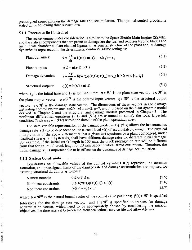
preassignedconstraintson the damagerate andaccumulation.The optimal control problem isstated in the following three subsections.
5.1.1 Process to Be Controlled
The rocket engine under consideration is similar to the Space Shuttle Main Engine (SSME),and the critical components that are prone to damage are the fuel and oxidizer turbine blades andmain thrust chamber coolant channel ligament. A general structure of the plant and its damagedynamics is represented in the deterministic continuous-time setting as:
dxPlant dynamics: x -_-- = f(x(t),u(t)); X(to ) = Xo (5.1)
dt
Plant outputs: y(t) = g(x(t),u(t)) (5.2)
dvDamage dynamics: i" -= -- = h(v(t),q(x, t)); v(t o) = Vo; h > 0 'v't _ [t o, tf ] (5.3)
dt
Structural outputs: q(t) = h(x(t), u(t)) (5.4)
where t o is the initial time and tf is the final time; x _ _n is the plant state vector; y _ 5Rt is
the plant output vector, u _ _m is the control input vector; q _ 9_ p is the structural output
vector; v E ¢j_r is the damage state vector. The dimensions of these vectors in the damagemitigating Control system are: n=20, 1=10, m=2, p=7, and r=-3 based on the plant dynamic modelderived in Chapter 2 and the structural and damage models presented in Chapter 3. Thenonlinear differential equations (5.1) and (5.3) are assumed to satisfy the local Lipschitzcondition (Vidyasagar, 1992) within the domain of the plant operating range.
The state-variable representation of the damage model in Eq. (5.3) allows the instantaneous
damage rate _'(t) to be dependent on the current Ievel v(t) of accumulated damage. The physical
interpretation of the above statement is that a given test specimen or a plant component, underidentical stress-strain hysteresis, shall have different damage rates for different initial damage.
For example, if the initial crack length is 100 mm, the crack propagation rate will be differentfrom that for an initial crack length of 20 mm under identical stress excursions. Therefore, the
initial damage v o is important due to its effects on the dynamics of damage accumulation.
5.1.2 System Constraints ...... ....
Constraints on allowablevalues of the control variables u(t) represent the actuator
saturation, and preassigned limits of the damage rate and damage accumulation are imposed forassuring structural durability as follows:
Natural bounds: 0 < u(t) < o_
Nonlinear constraints: 0 < h(v(t),q(x(t),t)) < _(t)
Nonlinear constraints: (v(tf) - Vo) < F
(5.5)(5.6)
(5.7)
where tx e _m is the natural bound vector of the control valve positions; I_(t) e 9_ r is specified
tolerances for the damage rate vector; and F E _r is specified tolerances for damageaccumulation vector, which need to be appropriately chosen by considering the missionobjectives, the time interval between maintenance actions, service life and allowable risk.
58
\
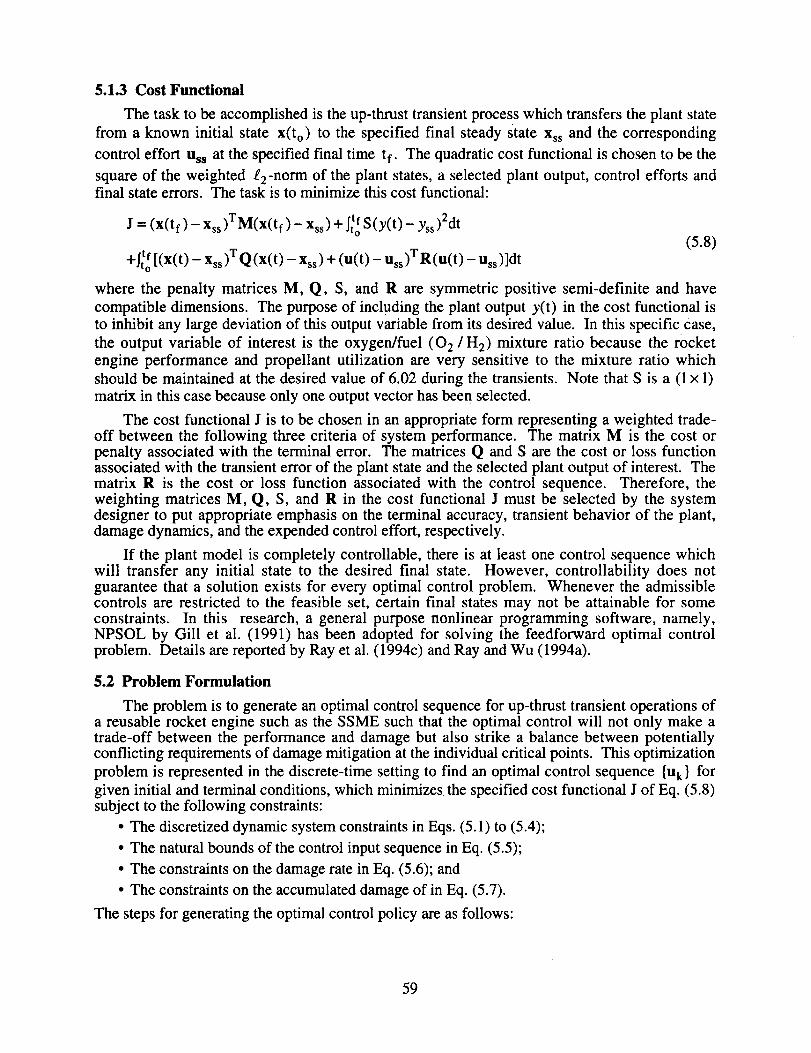
5.1.3 Cost Functional
The task to be accomplished is the up-thrust transient process which transfers the plant state
from a known initial state x(t o) to the specified final steady state Xss and the corresponding
control effort Uss at the specified final time tf. The quadratic cost functional is chosen to be the
square of the weighted £2-n°rm of the plant states, a selected plant output, control efforts andfinal state errors. The task is to minimize this cost functional:
J = (x(tf) - Xss)TM(x(t f) - Xss) + _of S(y(t) - Yss)2dt(5.8)
+J_of [(x(t) - Xss)XQ(x(t) - Xss) + (u(t) - Uss)r R (u(t) - Uss)]dt
where the penalty matrices M, Q, S, and R are symmetric positive semi-definite and have
compatible dimensions. The purpose of including the plant output y(t) in the cost functional is
to inhibit any large deviation of this output variable from its desired value. In this specificcase,
the output variable of interest is the oxygen/fuel (0 2 /H2) mixture ratio because the rocket
engine performance and propellant utilization are very sensitive to the mixture ratio which
should be maintained at the desired value of 6.02 during the transients. Note that S is a (1 x 1)
matrix in this case because only one output vector has been selected.
The cost functional J is tO be chosen in an appropriate form representing a weighted trade-off between the following three criteria of system performance. The matrix M is the cost orpenalty associated with the terminal error. The matrices Q and S are the cost or loss functionassociated with the transient error of the plant state and the selected plant output of interest. Thematrix R is the cost or loss function associated with the control sequence. Therefore, theweighting matrices M, Q, S, and R in the cost functional J must be selected by the systemdesigner to put appropriate emphasis on the terminal accuracy, transient behavior of the plant,damage dynamics, and the expended control effort, respectively.
If the plant model is completely controllable, there is at least one control sequence whichwill transfer any initial state to the desired final state. However, controllability does notguarantee that a solution exists for every optimal control problem. Whenever the admissiblecontrols are restricted to the feasible set, certain final states may not be attainable for someconstraints. In this research, a general purpose nonlinear programming software, namely,NPSOL by Gill et al. (1991) has been adopted for solving the feedforward optimal controlproblem. Details are reported by Ray et al. (1994c) and Ray and Wu (1994a).
5.2 Problem Formulation
The problem is to generate an optimal control sequence for up-thrust transient operations ofa reusable rocket engine such as the SSME such that the optimal control will not only make atrade-off between the performance and damage but also strike a balance between potentiallyconflicting requirements of damage mitigation at the individual critical points. This optimization
problem is represented in the discrete-time setting to find an optimal control sequence {Uk} for
given initial and terminal conditions, which minimizes the specified cost functional J of Eq. (5.8)subject to the following constraints:
• The discretized dynamic system constraints in Eqs. (5.1) to (5.4);
• The natural bounds of the control input sequence in Eq. (5.5);
• The constraints on the damage rate in Eq. (5.6); and
• The constraints on the accumulated damage of in Eq. (5.7).
The steps for generating the optimal control policy are as follows:
59

Minimizei
Subjectto:
and the constraints
N-1
J(fik) = xNTMXN + Ek=o
Xk+ 1 = X k + ftk+l f(x(t),u(t))dt;Jt k
Yk = g(Xk'Uk);
Vk+ 1 = v k + S_k+Jh(v(t),q(t))dt;
qk = _(Xk,Uk);
are;
O<fik <(_k
0 _<h(Vk,q(xk,tk)) < 13k
(VN - Vo) < F
[ikTQik + SYk 2 + fikTRfik]Atk
Xk = X(tk)
Uk = U(t k)
Vk = v(t k)
k=l, 2, ...,N
(5.9)
(5.10)
(5.11)
(5.12)
(5.13)
(5.14)
(5.15)
(5.16)
where N is the total number of discretized steps which represent the period from the initial time
t o to the final time tf; At k is the (possibly) non-uniform time interval, At k = tk+ 1 - t k, for
k=l, 2, to N; x k E _n×N is the plant state vector; Yk _9_exN is the plant output vector;
ll k E _mxN is the control input vector; v k e _rxN is the damage state vector; qk E _pxN is the
structural output vector; 6tk E _mxN is the normalized natural bound vector of the valve
positions; _k E 9_ r×N is specified tolerances for the damage rate vector; F e 9_r is specified
tolerances for accumulated damage vector; Xk E _n×N is the normalized deviations of plant
state vector; Yk E _t_lxN is the normalized deviations of selected plant output scalar which is
oxygen/fuel (O 2 / H 2) mixture ratio, the second component of the plant output vector Yk as seen
below in Eq. (5.17c); Uk e _rnxN is the normalized deviations of control input vector. The
definition of the above normalized vectors for k=l, 2, to N are given as:
• " 1 2 .-,X_] i=l, 2, n (5.17a)i Xk = [Xk,Xk,. ...,--(xL-x s)/Xss1 2, 3 e (5.17b)Yk = y2 _ y2 s Yk = [Yk,Yk Yk,'",Yk]
_i k = (Uik _ iUss) / Ussi I! k = [ul,u 2 ,...,u_ n ] i=l, 2, ..., m (5.17c)
For simplicity, the matrices M, Q, S and R are chosen to be diagonal and constant.Furthermore, the matrices M, Q and R are normalized according to the non-dimensional vectors
Xk, and fik in the cost functional J as described in Eq. (5.9).
Qnxn 'n+ 3_ Diag([l'l'C33'l'" 1]) suchthat trace(Q)= 1
S -- CSQ
fc,,-, "x
Rm×m =_-?--_AI m suchthat trace(R)=CRQ
Mn× n = CMQ x Qnxn such that trace(M) = CMQ
(5.18a)
(5.18b)
(5.18c)
(5.18d)
60
where the scalarconstants, CMQ, CSQ and CRQ in the weighting matrices M, S and R
represent their respective importance relative to the weighting matrix Q. This approach reducesthe variety of choices for weighting matrices. The diagonal elements of the weighting matrix Qshould be different because they correspond to the respective plant state variables which are not
equally important for performance. In the present model, the main combustor pressure which isthe third plant state variable is strongly related to the rocket engine performance. Therefore, the
third diagonal element of Q is chosen to be larger than others, i.e., C33 > 1 in Eq. (5.18a).
For solving the nonlinear optimization problem, the scalar weighting parameters in matrices
M, Q, S and R are chosen as C33 = 30; CSQ = 0.06; CRQ = 0.002 and CMQ = 0. The optimal
decision variables to be identified are the control inputs sequence {u k } having the dimension of
m x N for k=l, 2, ..., N. To accurately capture the fast dynamic response at an early stage ofthe transients, time steps Atk are chosen to be non-uniform as follows:
At k = c Atk_ 1 (5.19)
where constant c> 1 is the incremental ratio of two consecutive time steps. This setting of non-uniform time steps enhances the computational efficiency of numerical optimization process byreducing the total number steps of N (i.e., the dimension of the decision vector in optimization)
for the same period ( tf - to) without any significant loss of solution accuracy.
5.3 Optimization Results And Discussion
The purpose of these optimization studies is to examine the dynamic performance ofreusable rocket engines and the fatigue and creep damage in the critical components. Based onthe optimal control policy, the transients of the process variables and the resulting damage in the
critical components were obtained by manipu!ating the two oxidizer valves in Fig. 2.1. Therocket engine is maneuvered from the initial equilibrium state of chamber pressure at 2700 psiand mixture ratio of 6.02 to the new equilibrium state of chamber pressure at 3000 psi and thesame mixture ratio of 6.02 in 300 ms. The control commands to the two preburner oxidizervalves are updated at 37 discrete time instants (i.e., N=37) in which the parameters in Eq. (5.19)were selected as: c=1.035 and zxh=0.3 ms. The cost functional to be minimized is based on the
deviations from the final equilibrium state at 3000 psi.
Optimization was carried out under different damage rate constraints and different initialdamage in the critical plant components, namely, fuel turbine blades, oxidizer turbine blades, andthe coolant channel ligament in the main thrust chamber. Pertinent results are presented in thissection for four scenarios:
(i) Different creep damage constraints and a fixed initial creep damage in the ligament;
(ii) Different initial creep damage and a fixed creep damage constraint on the ligament;
(iii) Different fatigue damage constraints and a fixed initial fatigue damage on the fuel andoxidizer turbine blades; and
(iv) Different initial fatigue damage and a fixed fatigue damage constraint on the fuel andoxidizer turbine blades.
In the first two scenarios, no fatigue damage constraints were imposed on the fuel and oxidizerturbine blades, and the initial fatigue damage therein was held fixed. Optimization studies werealso conducted under different fatigue damage constraints and initial fatigue damage in the fueland oxidizer turbine blades. These results, corresponding to the last two scenarios, are extensionof those reported in a previous publication (Dai and Ray, 1994b) where no creep damageconstraints were imposed on the coolant channel, and the initial creep damage was held fixed.
61
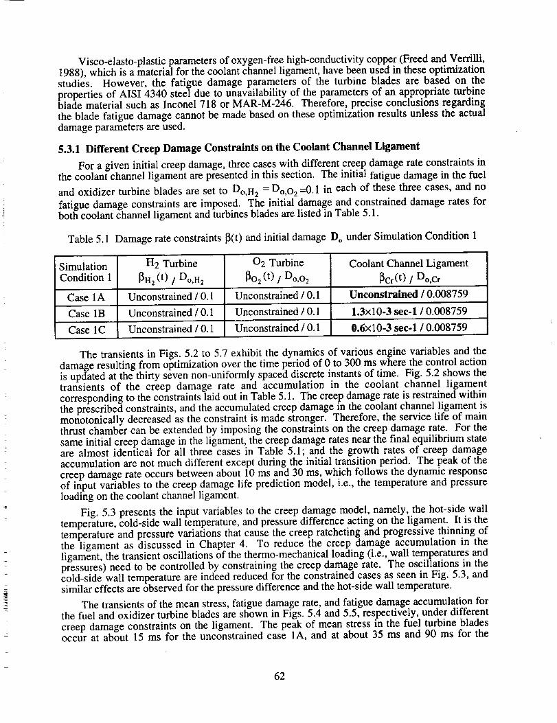
Visco-elasto-plasticparametersof oxygen-freehigh-conductivitycopper(FreedandVerrilli,1988),which is a materialfor thecoolantchannelligament,havebeenusedin theseoptimizationstudies. However, the fatigue damageparametersof the turbine blades are basedon thepropertiesof AISI 4340steeldue to unavailability of theparametersof anappropriateturbinebladematerial suchasInconel 718 or MAR-M-246. Therefore,preciseconclusionsregardingthe bladefatigue damagecannotbemadebasedon theseoptimization resultsunlesstheactualdamageparametersareused.
5.3.1 Different Creep Damage Constraints on the Coolant Channel Ligament
For a given initial creep damage, three cases with different creep damage rate constraints in
the coolant channel ligament are presented in this section. The initial fatigue damage in the fuel
and oxidizer turbine blades are set to Do,H 2 = Do,02 =0.1 in each of these three cases, and no
fatigue damage constraints are imposed. The initial damage and constrained damage rates forboth coolant channel ligament and turbines blades are listed in Table 5.1.
Table 5.1 Damage rate constraints _(t) and initial damage D O under Simulation Condition 1
Simulation H2 Turbine 02 Turbine Coolant Channel Ligament
Condition 1 1382 (t) / Do,H2 _o2 (t) / Do,o2 _Cr(t) / Do,c r
Case 1A Unconstrained / 0.1 Unconstrained / 0.1 Unconstrained / 0.008759
Case 1B Unconstrained / 0.1 Unconstrained / 0.1 1.3x10⁻³ see-1 / 0.008759
Case 1C Unconstrained / 0.1 Unconstrained / 0.1 0.6x10⁻³ see-1 / 0.008759
The transients in Figs. 5.2 to 5.7 exhibit the dynamics of various engine variables and thedamage resulting from optimization over the time period of 0 to 300 ms where the control actionis updated at the thirty seven non-uniformly spaced discrete instants of time. Fig. 5.2 shows thetransients of the creep damage rate and accumulation in the coolant channel ligamentcorresponding to the constraints laid out in Table 5.1. The creep damage rate is restrained withinthe prescribed constraints, and the accumulated creep damage in the coolant channel ligament ismonotonically decreased as the constraint is made stronger. Therefore, the service life of mainthrust chamber can be extended by imposing the constraints on the creep damage rate. For thesame initial creep damage in the ligament, the creep damage rates near the final equilibrium stateare almost identical for all three cases in Table 5.1; and the growth rates of creep damageaccumulation are not much different except during the initial transition period. The peak of thecreep damage rate occurs between about 10 ms and 30 ms, which follows the dynamic responseof input variables to the creep damage life prediction model, i.e., the temperature and pressureloading on the coolant channel ligament.
Fig. 5.3 presents the input variables to the creep damage model, namely, the hot-side wall
temperature, cold-side wall temperature, and pressure difference acting on the ligament. It is thetemperature and pressure variations that cause the creep ratcheting and progressive thinning ofthe ligament as discussed in Chapter 4. To reduce the creep damage accumulation in theligament, the transient oscillations of the thermo-mechanical loading (i.e., wall temperatures andpressures) need to be controlled by constraining the creep damage rate. The oscillations in thecold-side wall temperature are indeed reduced for the constrained cases as seen in Fig. 5.3, andsimilar effects are observed for the pressure difference and the hot-side wall temperature.
The transients of the mean stress, fatigue damage rate, and fatigue damage accumulation forthe fuel and oxidizer turbine blades are shown in Figs. 5.4 and 5.5, respectively, under differentcreep damage constraints on the ligament. The peak of mean stress in the fuel turbine bladesoccur at about 15 ms for the unconstrained case 1A, and at about 35 ms and 90 ms for the
62
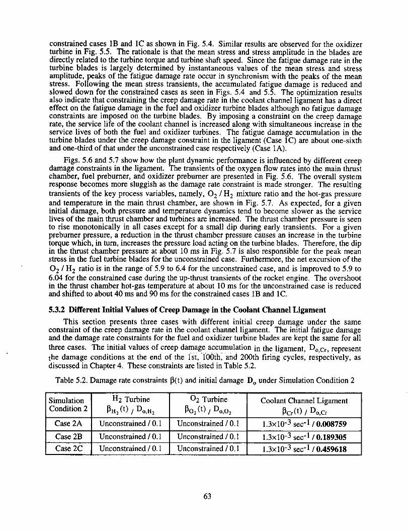
constrainedcases1Band 1Casshownin Fig. 5.4. Similar resultsareobservedfor the oxidizerturbine in Fig. 5.5. The rationaleis that themeanstressandstressamplitudein the bladesaredirectly relatedto theturbinetorqueandturbineshaftspeed.Sincethefatiguedamagerate in theturbine blades is largely determinedby instantaneousvaluesof the mean stressand stressamplitude,peaksof the fatiguedamagerateoccur in synchronismwith the peaksof the meanstress. Following the meanstresstransients,the accumulatedfatigue damageis reducedandsloweddown for theconstrainedcasesasseenin Figs. 5.4 and5.5. The optimization resultsalsoindicatethatconstrainingthecreepdamageratein thecoolantchannelligamenthasa directeffect on the fatiguedamagein the fuel andoxidizer turbinebladesalthoughno fatigue damageconstraintsare imposedon the turbineblades. By imposingaconstrainton the creepdamagerate,the servicelife of thecoolantchannelis increasedalongwith simultaneousincreasein theservicelives of both the fuel andoxidizer turbines. The fatigue damageaccumulationin theturbinebladesunderthe creepdamageconstraintin the ligament(Case1C)areaboutone-sixthandone-thirdof thatundertheunconstrainedcaserespectively(Case1A).
Figs. 5.6and5.7 showhow theplantdynamicperformanceis influencedby different creepdamageconstraintsin the ligament. The transientsof theoxygenflow ratesinto the mainthrustchamber,fuel preburner,andoxidizerpreburnerarepresentedin Fig. 5.6. The overall systemresponsebecomesmoresluggishasthedamagerateconstraintis madestronger.The resultingtransientsof the key processvariables,namely, 0 2 / H 2 mixture ratio and the hot-gas pressure
and temperature in the main thrust chamber, are shown in Fig. 5.7. As expected, for a giveninitial damage, both pressure and temperature dynamics tend to become slower as the servicelives of the main thrust chamber and turbines are increased. The thrust chamber pressure is seento rise monotonically in all cases except for a small dip during early transients. For a givenpreburner pressure, a reduction in the thrust chamber pressure causes an increase in the turbinetorque which, in turn, increases the pressure load acting on the turbine blades. Therefore, the dipin the thrust chamber pressure at about 10 ms in Fig. 5.7 is also responsible for the peak meanstress in the fuel turbine blades for the unconstrained case. Furthermore, the net excursion of the
0 2 / H 2 ratio is in the range of 5.9 to 6.4 for the unconstrained case, and is improved to 5.9 to
6.04 for the constrained case during the up-thrust transients of the rocket engine. The overshootin the thrust chamber hot-gas temperature at about 10 ms for the unconstrained case is reducedand shifted to about 40 ms and 90 ms for the constrained cases 1B and 1C.
5.3.2 Different Initial Values of Creep Damage in the Coolant Channel Ligament
This section presents three cases with different initial creep damage under the sameconstraint of the creep damage rate in the coolant channel ligament. The initial fatigue damageand the damage rate constraints for the fuel and oxidizer turbine blades are kept the same for all
three cases. The initial values of creep damage accumulation in the ligament, Do,or, represent
the damage conditions at the end of the 1st, rl00th, and 200th firing cycles, respectively, as
discussed in Chapter 4. These constraints are listed in Table 5.2.
Table 5.2. Damage rate constraints 13(0 and initial damage D O under Simulation Condition 2
Simulation H2 Turbine 02 Turbine Coolant Channel Ligament
Condition 2 _H 2 (t) / Do,H2 _O2 (t) / Do,o2 _Cr(t) / Do,c r
Case 2A Unconstrained / 0.1 Unconstrained / 0.1 1.3× 10 -3 sec- 1 / 0.008759
Case 2B Unconstrained / 0.1 Unconstrained / 0.1 1.3x10 -3 sec -1 / 0.189305
Case 2C Unconstrained / 0.1 Unconstrained / 0.1 i.3x10 -3 sec -1 / 0.459618
63
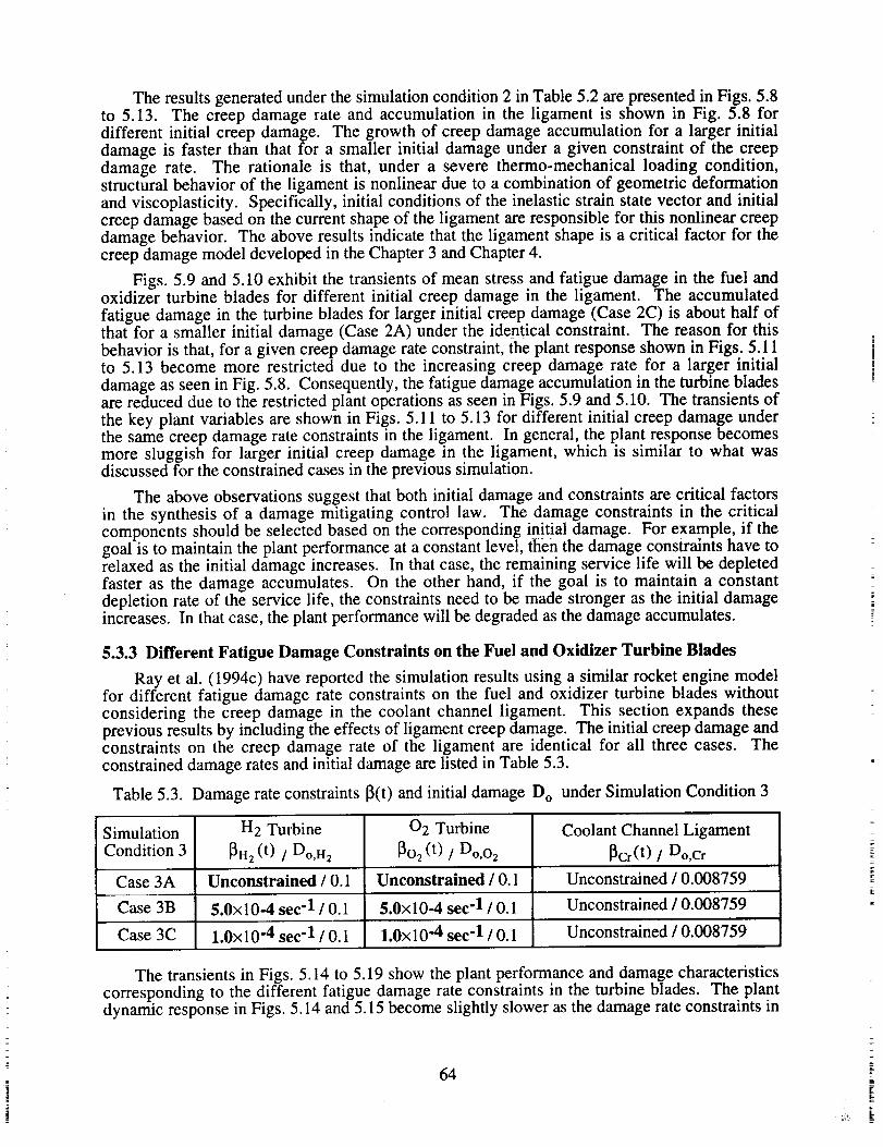
The results generated under the simulation condition 2 in Table 5.2 are presented in Figs. 5.8to 5.13. The creep damage rate and accumulation in the ligament is shown in Fig. 5.8 fordifferent initial creep damage. The growth of creep damage accumulation for a larger initialdamage is faster than that for a smaller initial damage under a given constraint of the creepdamage rate. The rationale is that, under a severe thermo-mechanical loading condition,structural behavior of the ligament is nonlinear due to a combination of geometric deformationand viscoplasticity. Specifically, initial conditions of the inelastic strain state vector and initialcreep damage based on the current shape of the ligament are responsible for this nonlinear creepdamage behavior. The above results indicate that the ligament shape is a critical factor for thecreep damage model developed in the Chapter 3 and Chapter 4.
Figs. 5.9 and 5.10 exhibit the transients of mean stress and fatigue damage in the fuel andoxidizer turbine blades for different initial creep damage in the ligament. The accumulated
fatigue damage in the turbine blades for larger initial creep damage (Case 2C) is about half ofthat for a smaller initial damage (Case 2A) under the identical constraint. The reason for thisbehavior is that, for a given creep damage rate constraint, the plant response shown in Figs. 5.11to 5.13 become more restricted due to the increasing creep damage rate for a larger initial
damage as seen in Fig. 5.8. Consequently, the fatigue damage accumulation in the turbine bladesare reduced due to the restricted plant operations as seen in Figs. 5.9 and 5.10. The transients of
the key plant variables are shown in Figs. 5.11 to 5.13 for different initial creep damage underthe same creep damage rate constraints in the ligament. In general, the plant response becomesmore sluggish for larger initial creep damage in the ligament, which is similar to what wasdiscussed for the constrained cases in the previous simulation.
The above observations suggest that both initial damage and constraints are critical factorsin the synthesis of a damage mitigating control law. The damage constraints in the criticalcomponents should be selected based on the corresponding initial damage. For example, if thegoal is to maintain the plant performance at a constant level, then the damage constraints have torelaxed as the initial damage increases. In that case, the remaining service life will be depleted
faster as the damage accumulates. On the other hand, if the goal is to maintain a constantdepletion rate of the service life, the constraints need to be made stronger as the initial damageincreases. In that case, the plant performance will be degraded as the damage accumulates.
5.3.3 Different Fatigue Damage Constraints on the Fuel and Oxidizer Turbine Blades
Ray et al. (1994c) have reported the simulation results using a similar rocket engine modelfor different fatigue damage rate constraints on the fuel and oxidizer turbine blades withoutconsidering the creep damage in the coolant channel ligament. This section expands theseprevious results by including the effects of ligament creep damage. The initial creep damage andconstraints on the creep damage rate of the ligament are identical for all three cases. Theconstrained damage rates and initial damage are listed in Table 5.3.
Table 5.3. Damage rate constraints 13(t) and initial damage D O under Simulation Condition 3
Simulation H2 Turbine 02 Turbine Coolant Channel Ligament
Condition 3 13H2(t) / Do,H2 _o2 (t) / Do,o2 _Cr(t) / Do,or
Case 3A Unconstrained / 0.1 Unconstrained / 0.1 Unconstrained / 0.008759
Case 3B 5.0x10⁻⁴ see "1 / 0.1 5.0× 10⁻⁴ sec "1 / 0.1 Unconstrained / 0.008759
Case 3C 1.0xl0 "4 see "1 / 0.1 1.0xl0 "4 sec -1 / 0.1 Unconstrained / 0.008759
The transients in Figs. 5.14 to 5.19 show the plant performance and damage characteristicscorresponding to the different fatigue damage rate constraints in the turbine blades. The plantdynamic response in Figs. 5.14 and 5.15 become slightly slower as the damage rate constraints in
64
[
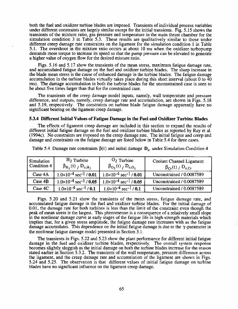
both the fuel and oxidizer turbine blades are imposed. Transients of individual process variablesunder different constraints are largely similar except for the initial transients. Fig. 5.15 shows thetransients of the mixture ratio, gas pressure and temperature in the main thrust chamber for thesimulation condition 3 in Table 5.3. These results are qualitatively similar to those underdifferent creep damage rate constraints on the ligament for the simulation condition 1 in Table
5.1. The overshoot in the mixture ratio occurs at about 10 ms when the oxidizer turbopumpdemands more torque to increase its speed so that the pump pressure can be elevated to generatea higher value of oxygen flow for the desired mixture ratio.
Figs. 5.16 and 5.17 show the transients of the mean stress, maximum fatigue damage rate,and accumulated fatigue damage on the fuel and oxidizer turbine blades. The sharp increase inthe blade mean stress is the cause of enhanced damage in the turbine blades. The fatigue damageaccumulation in the turbine blades virtually takes place during this short interval (about 0 to 40ms). The damage accumulation in both the turbine blades for the unconstrained case is seen tobe about five times larger than that for the constrained case.
The transients of the creep damage model inputs, namely, wall temperature and pressuredifference, and outputs, namely, creep damage rate and accumulation, are shown in Figs. 5.18and 5.19, respectively. The constraints on turbine blade fatigue damage apparently have nosignificant bearing on the ligament creep damage.
5.3.4 Different Initial Values of Fatigue Damage in the Fuel and Oxidizer Turbine Blades
The effects of ligament creep damage are included in this section to expand the results ofdifferent initial fatigue damage on the fuel and oxidizer turbine blades as reported by Ray et al.(1994c). No constraints are imposed on the creep damage rate. The initial fatigue and creep anddamage and constraints on the fatigue damage are listed below in Table 5.4 for three cases.
Table 5.4 Damage rate constraints 13(0 and initial damage D O under Simulation Condition 4
Simulation H2 Turbine 02 Turbine Coolant Channel Ligament
Condition 4 [_H2 (t) / Do,H2 [302 (t) / Do,o2 _Cr(t) / Do,c r
Case 4A 1.0×10 -4 sec -1 / 0.01 1.0xl0 -4 sec -1 / 0.01 Unconstrained / 0.0087589
Case 4B 1.0xl0 -4 sec -1 / 0.05 1.0xl0 -4 sec -1 / 0.05 Unconstrained / 0.0087589
Case 4C 1.0xl0 -4 sec -1 / 0.1 1.0xl0 °4 sec -1 / 0.1 Unconstrained / 0.0087589
Figs. 5.20 and 5.21 show the transients of the mean stress, fatigue damage rate, andaccumulated fatigue damage in the fuel and oxidizer turbine blades. For the initial damage of0.01, the damage rate for both turbines is less than the limit of the constraint even though thepeak of mean stress is the largest. This phenomenon is a consequence of a relatively small slopein the nonlinear damage curve at early stages of the fatigue life in high-strength materials whichimplies that, for a given stress amplitude, the fatigue damage rate increases with as the fatiguedamage accumulates. This dependence on the initial fatigue damage is due to the T-parameter inthe nonlinear fatigue damage model presented in Section 3.1.
The transients in Figs. 5.22 and 5.23 show the plant performance for different initial fatiguedamage in the fuel and oxidizer turbine blades, respectively. The overall system responsebecomes slightly sluggish as the initial damage on both the turbine blades increase for the reasonstated earlier in Section 5.3.2. The transients of the wall temperature, pressure difference acrossthe ligament, and the creep damage rate and accumulation of the ligament are shown in Figs.5.24 and 5.25. The observation is that different values of initial fatigue damage on turbineblades have no significant influence on the ligament creep damage.
65
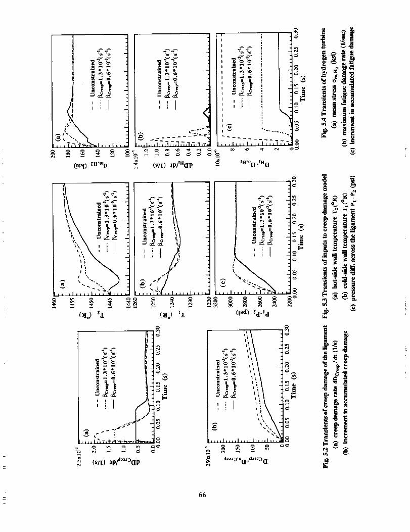
I
I
IIIII
I
I
Il
I I
_., ".,. \,,,, _,L_._.,k_.,,,,,,,,
• •
I I
<
I,,, i, ,, t,,, t,, ,1,, ,1,; ,'t,_
j I
_ ,_; . _ _ _ _
(!S_l) zH'm9 _ff: (s/I) _pfa(lp
I IL
';Ii ;
_H'O(i__ .rX(l
!
I
I
I
I
I
I
I
I
!
• '-4-!
!
I , , , I , , , l, , , I , , ,'_ _',_,._
o
%'_,
,_ _ :_..... _.... _,"; -..,,,,5,,,
()I o) _,L
. I
I
o _ _
(_Io) _£
-,?-.?
|
i'_
r._':_
'%,
I I i I i _ "4l "-I!
(!sd) _d._a
.¢.# ,,._m_ ',_
i I I i
' _,__,, I,, ,,I ,,,, I,, ,,I ,._
d_J3'o(] .d**'3(l
!
@
Le_
66
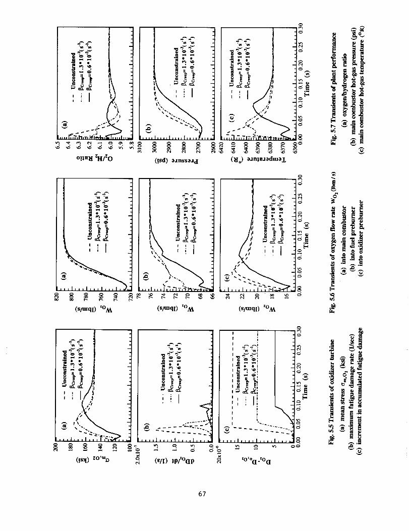
-I,,4
-I
":, .--4"4
'" / "
"1 X "] ./J -, ," /
h, ,, _l_,T,h,'n PIH',4-., I<_'_.,,.I
m _
.i]] _iN ,;I
_.,_'% *%
- ".-Z.Z.
(!sd) _Jnssa.M
oo
,.-. ,-.
u J
(s/mql) _°M
r
: ,C,_
_k 'k
r,.- r_ I_
(s/mql) _oM
I
.,.=4 _
_-_ _ " _'i ., ., ,'I ,';,TnT,_,'P,'_'a-- ."_..3 _ ._
°_
EE
ii _ _" S
,.,I; ;;l :¢_,,__/ - .
J'2"-. _
,,,,.','._.?,_-_._.
(s/_ql) _o_
i,_ _--,
m _
_ _ /:n
:_1/?
_ L'--. _,,,_,., i, ,.'_ ,_
I
__._-_ ._} -, ; !I ; I I
i,i_,l,,,,l,,,,l,,,,
(!sq) zo'_,_
ee_J_
c_
c_
'_ _< to ' o(]. _0Qe,/° (s/I) lp/°(Ip ¢_e_
¢J
t_ ¢1
i¢J
_,._
67
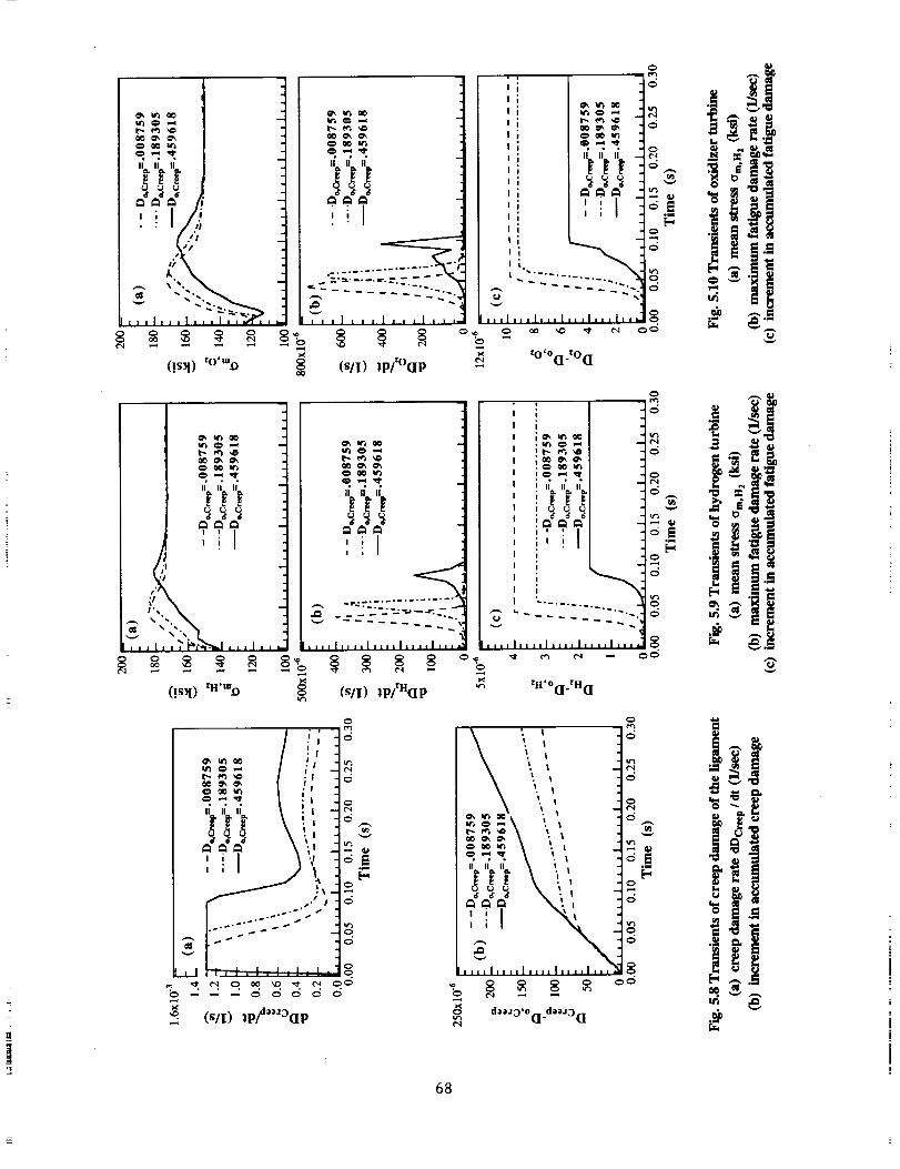
fla. lla. llo.
, i I /._
.-. _:.._
° 2",-:__(!S_l) _°'mD
i I i | ] i ! !
(s/I) _p/°oP
• • •
"+"+"+
_ ",',,.,
(Is+l) +w'_
i.
It_ t_ _,
,g& .,_4 '_p
I s
I-_,, - ,_-.......;., _--_•_ ° - __'_-.:- -- .
l,,,,l,,,il,_,_l,,,.l,,,,
(s/I) lp/ZX(I p
m
,' i I + +
(s/I) lp_+*_3(Ip
¢.q
68
C_
• i
i
i
i i I --_.
.
+O' Oo ._O(i
I,,,,I,,
' l
, iI
i "_"+"+I _ _
+,d ,d ,d -, ' t I
II
, _!
I
_'2"2"2"2"2"2":.::
_.I_,_,I,,,,I,,,.. .
ZH'OQ.;_H0
t_
,+,_.,_.\ ,., + +
0 0 _N
ddd \,.','!I "_._''_ "++'K N
_ \i _I .... I .... I .... h,,,I,,,_ _
_ = 8 * '°
._ _+_
&
° t+ ++-+
o
. _: .+i +.°[,-,
+ ++_ .
_ j|..,+m _
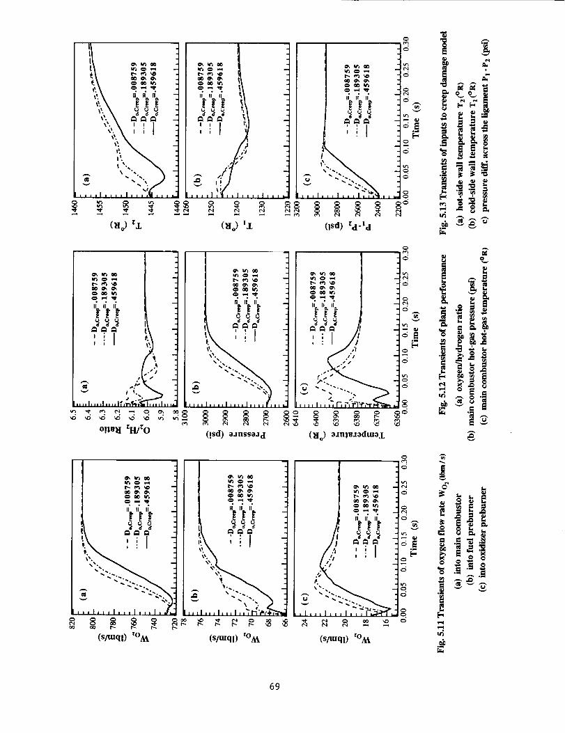
lt_ 0 ,,,,,i I1"_ 0 ,,-i
,_'. \ _ _ _ _ __'\ ' , I ' ' I rq , ,
"\'_J', '_' )_ 1 ,il
"-" "- "" \ / ""b"-.- ,,. e 8 -.:.-.,.... -..,,."._d --I ,,,,l,"i,,l,, I I, ""_ o°I I I I I I I I I I I I .
(N o) _,L (No) 13, (!sd) Zd-t d
8
i
i
•_- _
|!I ¢., ,c, _
,=, O0 Iw_
• ° •
1 "_"_"_6 ooo
t\ , ; I -t\ , : I -
% .,_ .% o,_.
% °_. ._ _°
I,,,1,,_1,,_1_,,I,_
I
U {..) U =
_._._,it ' ; I
%'. .
l" "'.'.%t,,, I,,, i,,, i, ,. P,",,.,._,_";'_
(s/mql) _°A£
O_ I_ O0
O_ O_ O__ O0 tr_
'_,_i_.'}.., :, I
I I I!
°1/
:\
Cq ("4 _
(stmql) _°A£
0
8 %
t.
o ',
_ _i _
_'-_
0 ° _
69
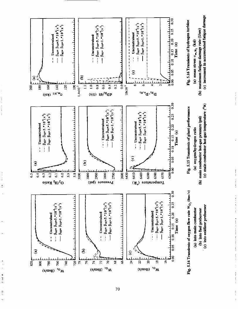
4
• [1} '_v
%%
cQ. o:1.
, , ]I a
i i i i i I i i
(!s_t) _W"D
._ • •
" 0
;;;) co>.cc_.
I I
.. _ _I, ,, I ,,, I,, ,1,...;';_ ;,
(s/[) _,pfH(i p 9
d
0 .
_,_
, , _ -
t. :
IIIl_ '"' I,,,,I,,_
o!l_l _H/_O
@
i i
II lit I t I
_ _ e e
_ m
i .,• ; -,
,,,,,,i
_, -_,_ _. ; -:-_.,
; I ' : ["I, ' J I -_
! -oI
I
"_ , -_
, ,',__,__,;_i=,.;,_ ..-, _
ZH'° 0 .ZH(I
0
cO. cO.
IU
v} -._ ..,
:ii!
===,=
ID
[- I1 II
O0 r"- t"_ f"
(s/_ql) _°M
" 1
I] I,, II II
! _ _ _1 o="" _-It _ II II
(s/_qi) _°M
", '7
%%
_-'.
_t,l,, ,,I
0¢,1
_sE
B
v
[...
70
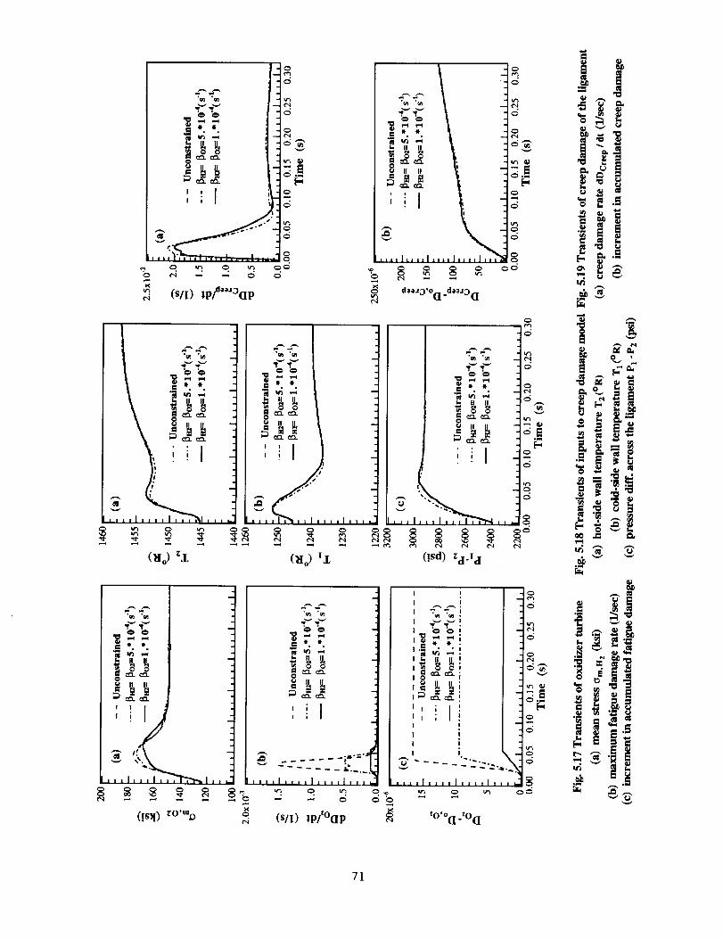
r"
lll_ll II i I11
l 'i_ , , I, , ,I , , ,]'t'_l , ,
(!s_l):0''9
(!sd) _d._d
I
I
i illllll
(s/I) iP/'°(IP
7l
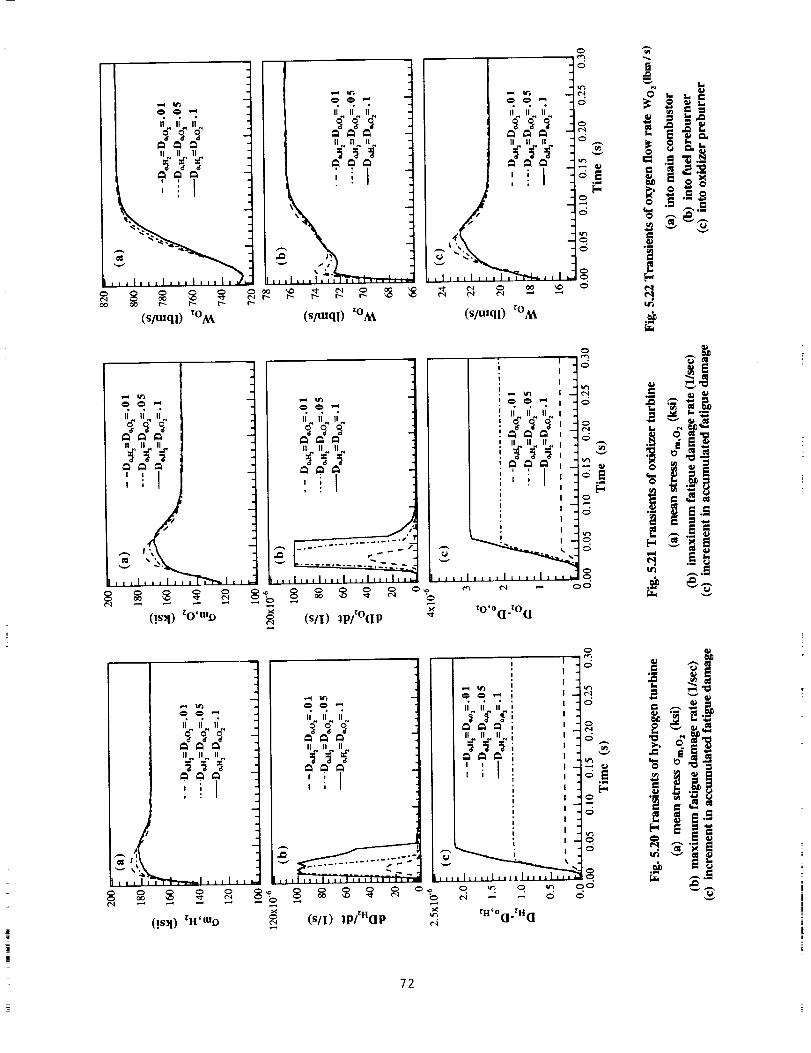
:!J
l,,,It
(s/mql) _oM
JlZII II I!
fff
, 'il £k " " '
-\i
(s/mql) _oM (s/mql) _oM
,;,,_,,__ _ _o_
/ o_ _._._,_.t <_
g¢-I
ddd
/._ ":__
(!s_l) _O'm_
II II II
fff
, , I
_ff_
'?,?,?; '.j
I
e_
'1°
[.,
.. ; _,
II,,l,,,I,IIIIIII [I .... ] .... I,,,,I ....
_ _ _ _ _ _ '::'_ _ _ - o,_x tO'O(i =0(io (s/I) _pf°(IP _ "
__._
,i ,i i
ddd
,,¢,,_,,¢, , I
i "
/
(!s_) ZlI'm_
II II II
fff
'_"'k'k
• ° , ,
II , . II !
, , I
I
!
.-. !
- - "_ (g - .:
(s/I) 1P[a(IP__ e.i rH'°(]'rH(l
f. _'_
_. _'_- _ _ .-.._
72
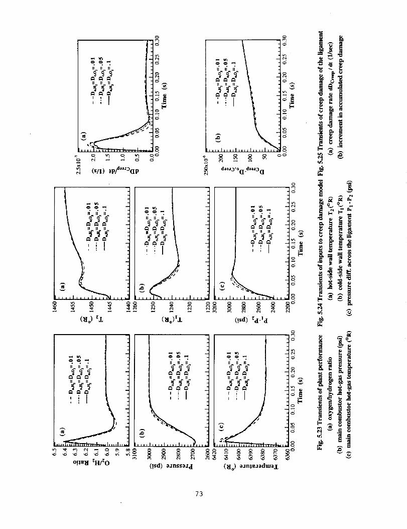
,_ irali li
II I! I_
II II II
I I
L_ 1.__"i ii l'lill i i-Ii|i ,.
(s/i) i liP
i -
i -
c5
-- t"4
°
, °
c_
0
c_
t¢3
f=,
'9,
II II II"
JJZII It
,-i-i
-ti-i
,..4,-2.
,,,,I,,,,I,,,,I,
d_aJ2_'o(i d+_J21Q
II II II
'.il
V3 _
II II II
'1 !
/.,, ,."l I,, ,I,-"i,,l,,,,I,,,,.
_ +_ o _ o(_o)t_
"2.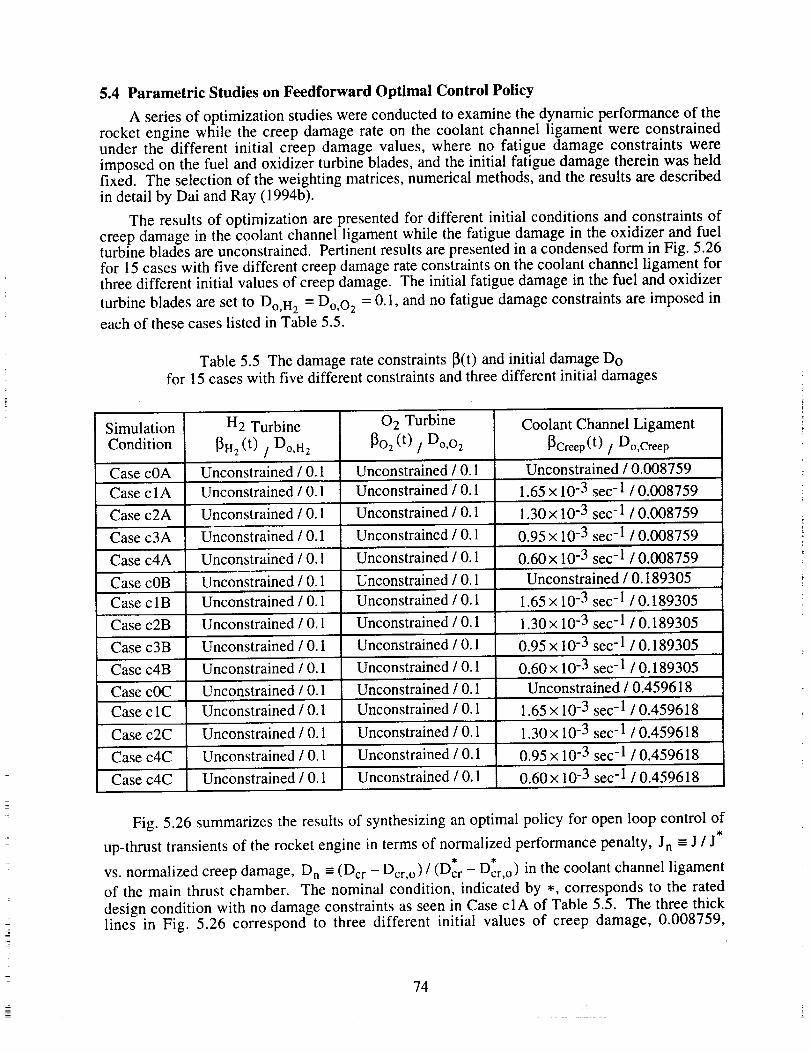
5.4 Parametric Studies on Feedforward Optimal Control Policy
A series of optimization studies were conducted to examine the dynamic performance of therocket engine while the creep damage rate on the coolant channel ligament were constrainedunder the different initial creep damage values, where no fatigue damage constraints wereimposed on the fuel and oxidizer turbine blades, and the initial fatigue damage therein was heldfixed. The selection of the weighting matrices, numerical methods, and the results are describedin detail by Dai and Ray (1994b).
The results of optimization are presented for different initial conditions and constraints ofcreep damage in the coolant channel ligament while the fatigue damage in the oxidizer and fuelturbine blades are unconstrained. Pertinent results are presented in a condensed form in Fig. 5.26for 15 cases with five different creep damage rate constraints on the coolant channel ligament forthree different initial values of creep damage. The initial fatigue damage in the fuel and oxidizer
turbine blades are set to Do,H2 = Do,O2 = 0.1, and no fatigue damage constraints are imposed ineach of these cases listed in Table 5.5.
Table 5.5 The damage rate constraints [3(t) and initial damage Do
for 15 cases with five different constraints and three different initial damages
SimulationCondition
Case c0A
H2 Turbine
_H 2 (t) / Do,H2
Unconstrained / 0. I
0 2 Turbine
[3o2 (t) / Do,o2
Coolant Channel Ligament
[3creep(t) / Do,creep
Unconstrained / 0.1 Unconstrained / 0.008759
Case c 1A Unconstrained / 0.1 Unconstrained / 0.1 1.65 x 10 -3 sec- 1 / 0.008759
Case c2A Unconstrained / 0.1 Unconstrained / 0.1 1.30 x 10⁻³ sec- 1 / 0.008759
Case c3A lJnconstrained / 0.1 Unconstrained / 0.1 0.95 x 10 -3 sec- 1 / 0.008759
Case c4A Unconstrained / 0.1" Unconstrained / 0.1
Case cOB
Case clB
Case c2B
Case c3B
Case c4B
Case c0C
0.60x 10 -3 sec -1 / 0.008759
Case c 1C
....Case c2C
Case c4C
Case c4C
Unconstrained / 0.1 Unconstrained / 0.1 Unconstrained / 0.189305
Unconstrained / 0.1 Unconstrained / 0.1 1.65 x 10 -3 sec- 1 / 0.189305
Unconstrained / 0.1 Unconstrained / 0.1 1.30 x 10 -3 sec" 1 / 0.189305
Unconstrained / 0.1 Unconstrained / 0.1 0.95 x 10 -3 sec- 1 / 0.189305
Unconstrained / 0.1 Unconstrained / 0.1 .... 0.60× 10 -3 sec -1 / 0.189305
Unconstrained / 0.1 Unconstrained / 0.1 Unconstrained / 0.459618
Unconstrained / 0.1 Unconstrained / 0.1 1.65 × 10 -3 sec-1 / 0.459618
Unconstrained / 0.1 Unconstrained / 0.1 1.30 x 10⁻³ sec- 1 / 0.459618
Unconstrained / 0.1 Unconstrained / 0. i 0.95 x 10 -3 sec- 1 / 0.459618
Unconstrained / 0.1 Unconstrained / 0.1 0.60 × 10 -3 sec- 1 / 0.459618
Fig. 5.26 summarizes the results of synthesizing an optimal policy for open loop control of
up-thrust transients of the rocket engine in terms of normalized performance penalty, Jn =- J / J*
vs. normalized creep damage, D n --=(Dcr - Dcr,o) / (Dcr - Dcr,o) in the coolant channel ligament
of the main thrust chamber. The nominal condition, indicated by *, corresponds to the rated
design condition with no damage constraints as seen in Case c 1A of Table 5.5. The three thicklines in Fig. 5.26 correspond to three different initial values of creep damage, 0.008759,
74
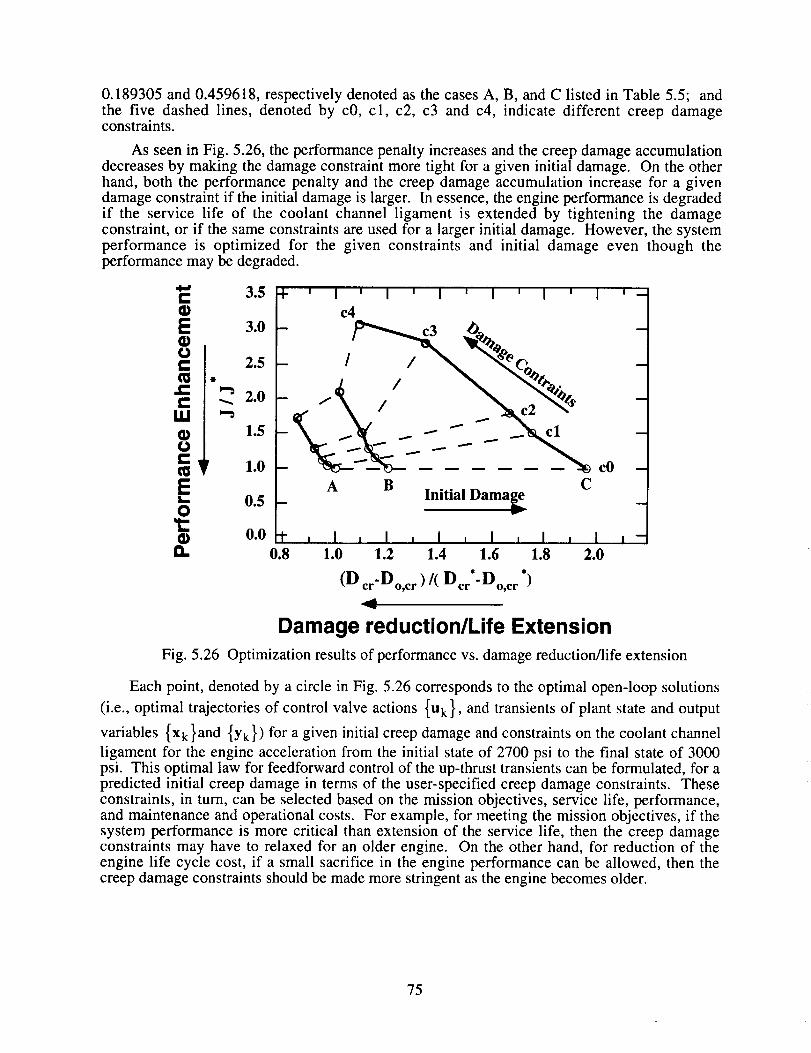
0.189305and0.459618,respectivelydenotedasthecasesA, B, andC listed in Table 5.5; andthe five dashed lines, denotedby cO,c l, c2, c3 and c4, indicate different creep damageconstraints.
As seenin Fig. 5.26, theperformancepenaltyincreasesandthecreepdamageaccumulationdecreasesby makingthedamageconstraintmoretight for a giveninitial damage.On theotherhand,both the performancepenaltyand the creepdamageaccumulationincreasefor a givendamageconstraintif the initial damageis larger. In essence,theengineperformanceis degradedif the service life of the coolant channel ligament is extendedby tightening the damageconstraint,or if thesameconstraintsareusedfor a largerinitial damage.However, thesystemperformance is optimized for the given constraints and initial damageeven though theperformancemaybedegraded.
tlJ
E LO
0.0I_. 0.8
3.5 ' I ' I ' I i I i I m I i _
c4
3.0 c3 -
2.5 1' /__¢Po_, -
1.5 -
1.0 cO -
0.5 Initial Dama_,.e - _
, I I I I I I I I I _ I I-1.0 1.2 1.4 1.6 1.8 2.0
(D cr-Do,cr )/( Dcr°-Do,cr *)
Damage reduction/Life ExtensionFig. 5.26 Optimization results of performance vs. damage reduction/life extension
Each point, denoted by a circle in Fig. 5.26 corresponds to the optimal open-loop solutions
(i.e., optimal trajectories of control valve actions {u k }, and transients of plant state and output
variables {x k }and {Yk}) for a given initial creep damage and constraints on the coolant channel
ligament for the engine acceleration from the initial state of 2700 psi to the final state of 3000psi. This optimal law for feedforward control of the up-thrust transients can be formulated, for apredicted initial creep damage in terms of the user-specified creep damage constraints. Theseconstraints, in turn, can be selected based on the mission objectives, service life, performance,and maintenance and operational costs. For example, for meeting the mission objectives, if thesystem performance is more critical than extension of the service life, then the creep damageconstraints may have to relaxed for an older engine. On the other hand, for reduction of theengine life cycle cost, if a small sacrifice in the engine performance can be allowed, then thecreep damage constraints should be made more stringent as the engine becomes older.
75

5.5 Simulation of the Damage Mitigating Control System on a Testbed
The feedforward control policy is generated in Section 5.2 to achieve optimal performance
of the rocket engine based on a nominal model of plant and damage dynamics. However,because of modeling uncertainties, sensor noise and external disturbances, the actual responsewill deviate from nominal trajectory when the plant is excited by the sequence of the feedforwardcontrol commands. Therefore, a feedback control system can be used to compensate for these
deviations. A robust output feedback controller has been synthesized to maintain the trajectories
of the plant output variables close to the respective nominal trajectories.
Feedforward and
Robust OutputFeedback Controller
and Model-based
Damage Predictor
Fig. 5.27 Schematic diagram of the simulation testbed operations
A simulation testbed has been established for evaluation of damage mitigating control
systems. The testbed, at this stage, consists of an Silicon Graphics (SGI) Indigo R-4000workstation, two 586-based and one 486-based PCs which are interconnected via ethernet asshown in Fig. 5.27. The SGI workstation has been used for off-line computations that includemodel development of both plant and structural & damage dynamics, and analysis and synthesis
of both feedforward and robust feedback control policies via nonlinear programming and g-
synthesis (Packard and Doyle, 1993), respectively. The 20th nonlinear plant dynamic model ofthe rocket engine is simulated on one of the PC-586s, which serves as the real plant. Both thefeedforward control policy and the linear robust output feedback control policy are implementedin the second PC-586 along with the analytical structural and life prediction models of the critical
components (i.e., fuel and oxidizer turbine blades and main thrust chamber coolant wall). Thissoftware for on-line life prediction and control is portable to other machines. All three machines
serve as display devices of the selected process and damage variables.
76
CHAPTER 6
SUMMARY, CONCLUSIONS, AND RECOMMENDATIONS FOR FUTURE WORK
This report investigates the feasibility of damage mitigating control of reusable rocketengines where the objective is to achieve optimized trade-off between the system performanceand structural durability. Summary and conclusions of this interdisciplinary research arepresented in Section 6.1. Future research for transfer of this space technology to the electricpower industry is recommended in Section 6.2.
6.1 Summary and Conclusions
A unified methodology has been proposed for analysis and synthesis of damage mitigatingcontrol systems for rocket engines by integrating the disciplines of thermo-fluid dynamics,mechanical structures, and mechanics of materials along with control and optimization ofdynamic systems. Research work in each of these disciplines are summarized and concluded inSections 6.1. ! to 6.1.3.
6.1.1 Plant Dynamic Model of a Reusable Rocket Engine
Plant dynamics of a rocket engine which is similar to the Space Shuttle Main Engine(SSME) have been modeled in Chapter 2 is to represent its steady-state and dynamiccharacteristics for damage prediction and synthesis of a damage mitigating control policy. The20th order, nonlinear, time-invariant and deterministic model is formulated in the state-spaceform, and numerical results are obtained by digital simulation.
Steady-state model results agree closely with those of a more detailed nonlinear model of theSSME reported by Rockwell (1989). Transient responses of the nonlinear plant model areobtained at the full load by initiating independent step disturbances in two input variables. Theresults show that the two control input valves, FPOV and OPOV, have significant effects on
0 2 [ H 2 mixture ratio and chamber pressure as discussed by Musgrave (1990). In particular, thechamber pressure is affected to a much greater extent due to the step change in the FPOV thanthat due to the OPOV. These results are useful for:
(i) Understanding the complex and highly interactive process dynamics;(ii) Providing the process variables (i.e., turbopump speed and torque, wall temperature and
pressure loading) for damage prediction in the critical plant components; and(iii) Investigating both feedforward and feedback system dynamic performance under various
operating conditions.
These results can also be used for prediction of potential operational and control problems ofreusable rocket engines.
6.1.2 Structural and Damage Model of the Combustion Chamber Wall
This report presents the development of a creep damage model in the coolant channelligament of the main thrust chamber during transient operations of a reusable rocket engine suchas the SSME. This damage model is based upon the theories of sandwich beam andviscoplasticity. The modeling approach consists of analyzing the incremental bulging-out andprogressive thinning of the ligament in each firing cycle by taking the effects of geometricdeformation into consideration.
A structural and damage model of the coolant channel wall for the main thrust chamber hasbeen analytically derived and subsequently validated in terms of single-cycle and multi-cyclestress-strain behavior by comparison with finite element models and experimental data for twodifferent materials, namely, OFHC copper and NARloy-Z. The predicted results are inagreement with those obtained from the finite element analyses and experimental observations.
77
The close agreement with the finite element models indicates that the proposed life predictionmodel can capture the failure mechanics (i.e., creep rupture) of the main thrust chamber wall bycalculating the mid-plane deflection of the ligament. This model has been proven to benumerically much more efficient than the finite element model with comparable accuracy.Validation of this model for both NARloy-Z and OFHC copper materials and its numerical
efficiency establish its credibility for on-line life prediction and damage mitigating control of arocket engine for which the finite-element model is not appropriate. To the best of the author'sknowledge, the proposed life prediction model is the only available model which is suitable forboth on-line life prediction and damage mitigating control.
The predicted life of the coolant channel wall is influenced by several factors including theligament material, configuration and design of the channel, chamber pressure, wall temperature,and loading cycle duration. These effects have been investigated through parametric studies, andthe following conclusions are derived:
1. The failure phenomena, regardless of whether the material is OFHC copper or NARloy-Z, are characterized by thinning of the center of the ligament. An OFHC copper ligament is
potentially more prone to damage because the thinout process accelerates leading to an abruptrupture. NARloy-Z materials show an improvement in cyclic life over the OFHC coppermaterial at a given thermo-mechanical loading. The deformation of an OFHC copper chamber ispredicted to be larger than for that for a less ductile NARloy-Z chamber, which is in agreementwith experimental observations.
2. Increasing the number of coolant channels is one of the feasible approaches to lifeextension of the main thrust chamber.
3. The pressure difference across the coolant channel ligament is a cause of the bulging-out
phenomenon, and the ligament thinning increases with the pressure difference.
4. Decreasing the coolant wall temperature is a possible solution to reduce thinning of themain thrust chamber wall. The thermally induced bending resulting from temperature difference
across the ligament tends to retard the bulging out process due to the pressure loading, andtherefore improves the service life of the main thrust chamber, especially for the OFHC coppermaterial.
5. The magnitude of the bulging-out and thinning of the coolant channel ligament of bothOFHC copper and NARloy-Z materials is depended on the duration of the loading cycle. Thebulging out process is more pronounced for the extended cycle than for the short loading cycle.
6.1.3 Integrated Life Extension and Control Synthesis
The benefits derived from damage mitigating control of reusable rocket engines, as
presented in this report, are summarized below:
• Maximum system performance of rocket engines can be achieved with increased
durability of the mechanical structures such that functional lives of critical components areincreased.
• On-line life prediction and damage mitigation, based on the available sensory andoperational information, will allow reusable rocket engines to be inexpensively maintained, and
safely and efficiently steered under diverse operating conditions.
The feasibility of applying this control concept to rocket engines such as the SSME has been
investigated in view of fatigue and creep damage in three critical components, namely, the fuelturbine, the oxidizer turbine, and the main thrust chamber. Based on the fatigue damage model
and the proposed creep damage model, an optimal feedforward policy has been synthesized foropen loop control of up-thrust transients of the rocket engine under the damage constraints on theabove three critical components.
78
The resultsof optimization studies demonstrate the interactive nature of fatigue damage inthe fuel and oxidizer turbine blades, and creep damage in the coolant channel ligament of themain thrust chamber. The damage accumulation in both coolant channel ligament and turbineblades are seen to be significantly influenced by their respective constraints and initial damage.It is observed that the initial damage in the critical components may have a significant impact onservice life extension of rocket engines. Therefore, in the synthesis of the control policy, boththe constraints and performance cost function need to be selected based on the knowledge of the
initial damage in the critical components.
Up-thrust transients of the rocket engine have been simulated for a brief period of 300 ms.Complete operations of a reusable rocket engine over its life include many such transients, andthe steady-state operation in a single flight may last for several hundreds of seconds. Althoughboth fatigue and creep damage rates during the steady state are smaller than those duringtransient operations, the total damage accumulation during steady state operations may not beinsignificant. Therefore, during one flight of a reusable rocket engine, the cumulative effects ofboth transient and steady state operations need to be considered for estimation of total damageaccumulation. The optimization studies presented in this report only consider a single point ineach of the three critical components. Simultaneous control of damage at several other critical
points in the rocket engine might be necessary for damage mitigation and life extension.However, this will make the optimization problem more complex as the dimension of the
damage vector will be large compared to the three-dimensional damage vector in the presentstudy.
6.2 Recommendations for Future Work
The concept of damage mitigation, presented in this report, is not restricted to control ofrocket engines. It can be applied to any system where structural durability is an important issue.Besides rocket engines, applications of damage mitigating control include a wide spectrum ofengineering applications such as fossil and nuclear plants for electric power generation, rotatingand fixed wing aircraft, automotive and truck engine/transmission systems, and large rollingmills. In each of these systems, damage mitigating control can enhance safety and productivity
accompanied by reduced life cycle cost.
For example, the availability of power plants often suffers from premature failures of steamgenerator tubes (due to corrosion-fatigue and creep), main steam and reheater steam pipelines(due to creep and fatigue), condenser tubes (due to stress corrosion cracking and flow-inducedvibration) and low pressure turbine blades (due to stress corrosion, erosion, and fatigue). Acontinuous-time damage model will allow timely warnings of these failures, and the resultingdecision and control actions may not only avoid an early shutdown but also improve
maintainability: A more complex application of the damage mitigation concept is start-up andscheduled shutdown of power plants, and take-off and landing of commercial aircraft, in whichthe damage information can be utilized for real-time plant control either in the fully automated
mode or with human operator(s) in the loop.
The concept of damage mitigating control is of significant importance to power andprocessing plants. Many components such as steam generators in conventional power andprocessing plants are exposed to high loads at elevated temperatures, and have been in usebeyond the design life of 30 to 40 years. Several preliminary investigations have shown that thecost of life extension of a typical fossil power plant may be only 20 to 30 percent of that of a newconstruction (Viswanathan, 1989). Therefore, the concept of damage mitigating control isideally suited to life extension of aging power plants under both steady state and transientoperations. The objective is to enhance plant performance, availability and maintainability whilesimultaneously reducing the structural damage to avoid unscheduled plant shutdown and repairas much as possible. This objective can be achieved via transfer of the technology of damagemitigating control for the rocket engines to power plant applications.
79
REFERENCES
Allen, D.H. and Beek, J.M., 1984, "On the Use of Internal State Variables in Thermoviscoplastic Constitutive
Equations," Symposum on Nonlinear Constitutive Relations for High Temperature Application, NASA LewisResearch Center, June 15-17, pp. 83-101.
Armstrong, W.H., 1979, "Structural Analysis of Cylindrical Thrust Chamber," Final Report, Volume I, NASA CR-159552, Contract NAS3-21361, NASA Lewis Research Center, March.
Armstrong, W.H., 1981, "Structural Analysis of Cylindrical Thrust Chamber," Final Report, Volume II, NASA CR-165241, Contract NAS3-21953, NASA Lewis Research Center, March.
Arnold, S.M., Robinson, D.N. and Saleeb, A.F., "Creep Buckling of Cylindrical Shell Under Variable Loading,"
Journal of Engineering Mechanics, V115, No. 5, May-August,, pp. 1054-1075
Arya, V.K., 1992, "Nonlinear Structural Analysis of Cylindrical Thrust Chambers Using Viscoplastic Models,"Journal of Propulsion and Power, Voi. 8, No. 3, May-June, pp. 598-604.
Arya, V.K. and Arnold, S.M., 1992, "Viscoplastic Analysis of an Experimental Cylindrical Thrust Chamber Liner,"AIAA Journal, Vol. 30, No. 3, March, pp. 781-789.
Blackburn, J.F., Reethof, G. and Shearer, J.L., 1960, Fluid Power Control, The technology press of Massachusetts
Institute of Technology, Dynamic Analysis and Control Laboratory.
Chen, K.S., Lindholm, U.S., Bodner, S.R. and Walker, K.P., 1984, "A Survey of Unified Constitutive Theories,"
Symposum on Nonlinear Constitutive Relations for High Temperature Application, 1984, NASA LewisResearch Center, Ohio, June 15-17, pp. 1-23.
Dai, X. and Ray, A., 1994a, "Damage-Mitigating Control of a Reusable Rocket Engine, Part 1: Life Prediction of theCombustion Coolant Wall," ASME Winter Annual Meeting, Chicago, November, and to be published in Journal
of Dynamic Systems, Measurement and Control., Trans. ASME.
Dai, X. and Ray, A., 1994b, "Damage-Mitigating Control of a Reusable Rocket Engine, Part 2: Formulation of an
Optimal Control Policy and Simulation," ASME Winter Annual Meeting, Chicago, November, and to bepublished in Journal of Dynamic Systems, Measurement and Control., Trans. ASME.
Duyar, A., Guo, T-H. and Merrill, W.C., 1990, "Space Shuttle Main Engine Model Identification," IEEE ControlSystem Magazine, Vol. 10, No. 4, pp. 59-65.
Duyar, A., Eldem, V., Merrill, W.C., and Guo, T-H., 1991, "State Space Representation of the Open-Loop Dynamicsof the Space Shuttle Main Engine," Journal of Dynamic Systems, Measurement, and Control, Trans. ASME.,December, Voi. 113, pp. 684-690.
Freed, A.D., 1988, "Structure of a Viscoplastic Theory," NASA TM-100749, Lewis Research Center, Cleveland,
Ohio, Prepared for the Summer Annual Meeting Symposium: Constitutive Equations and Life PredictionModels for High Temperature Applications, sponsored by ASME, Berkeley, California, June 20-22.
Freed, A.D. and Verrilli, M.J., 1988, "A viscoplastic Theory Applied to Copper," NASA TM-100831, Lewis
Research Center, prepared for the International Seminar on The Inelastic Behavior of Solids Models andUtilization, Sponsored by MECAMAT, Besancon, France, August 30 - September I.
Gill, P.E., Murray, W., Saunders, M.A. and Wright, M.H., 1991, NPSOL Version 4.06, Software DistributionCenter, Stanford University, Pato Alto, CA.
Hannum, N. P., Kasper, H.J. and Pavli, A.J., 1976, "Experimental and Theoretical Investigation of Fatigue Life inReusable Rocket Thrust Chambers," NASA TM X-73413, Lewis Research Center, July.
Kasper, H.J., 1984, "Thrust Chamber Life Prediction", NASA Conference Publication 2372, Advanced high pressure02/H2 technology, Proceedings of a conference held at George C. Marshall Flight Center, Huntsville, Alabama,
June 27-29, pp. 36-43.
Lorenzo, C.F. and Merrill, W.C., 1991a, "Life Extending Control: A Concept Paper," American Control Conference,
Boston, MA, June, pp. 1080-1095.
Lorenzo, C.F. and Merrill, W.C., 1991b, "An Intelligent Control System for Rocket Engines: Need, Vision, andIssues," Control Systems Magazine, Vol. 12, No. 1. January, pp. 42-46.
Luenberger, D.G., 1984, Linear and Nonlinear Programming, 2nd edition, Reading, Mass., Addison-Wesley, MenloPark, CA.
McDowell, D.L., 1992, "A Nonlinear Kinematic Hardening Theory for Cyclic Thermoplasticity and
Thermoviscoplasticity," International Journal of Plasticity, Vol. 8, pp. 695-728.
80
Musgrave, J.L., 1990, "Advanced Control Modes for Space Shuttle Main Engine," Conference on Advanced Earth-to Orbit Propulsion, Technology held at NASA George C. Marshall Space Flight Center, Marshall Space Flight
Center, Alabama, May 15-17.
Noll, T., Austin, E., Donley, S., Graham, G., Harris, T., Kaynes, I., Lee, B. and Sparrow, J., 1991, "Impact of ActiveControls Technology on Structural Integrity," 32nd AIAA/ASME/ASCE/AHS/ASC Structures, Structural
Dynamics, and Materials Conference, Baltimore, MD, April, pp. 1869-1878.
Packard, A. and Doyle, J., 1993, "The Complex Structured Singuler Value," Automatica, Vol 29. No. 1, pp. 71-109.
Pads, P.C., and Erdogan, F., 1963, "A Critical Analysis of Crack Propagation Laws," Journal of Basic Engineering,Trans. ASME, Vol. D85, pp. 528-534.
Porowski, J.S., O'Donnell, W.J., Badlani, M.L. and Kasraie, B., 1985, "Simplified Design and Life Prediction ofRocket Thrust Chambers," Journal of Spacecraft, 1985, Vol. 22, March-April, pp. 181-187.
Pugh, C.E. and Robinson, D.N., 1978, "Some Trends in Constitutive Equation Model Development for High-Temperature Behavior of Fast-Reactor Structural Alloys," Journal of Nuclear Engineering and Design, Vol. 48,
pp. 269-276.
Quentmeyer, R.J., 1977, "Experimental Fatigue Life Investigation of Cylindrical Thrust Chambers," NASA TM X-73665, Lewis Research Center, July 1977.
Ray, A., 1976, Mathematical Modeling and digital Simulation of a Commercial Scale High Temperature Gas-Cooled Reactor (HTGR) Stream Power Plant, Ph.D. Dissertation in Mechanical Engineering, Northeastern
University, Boston, Massachusetts, June.
Ray, A. and H. F. Bowman, 1978, "Digital Simulation of a High Temperature Gas-Cooled Reactor (HTGR) SteamPower Plant," IEEE Trans. on Nuclear Science, August, pp. 1068-1077.
Ray, A., Wu, M-K., Carpino, M., Lorenzo, C., F., 1994a, "Damage-Mitigating Control of Mechanical Systems: PartI - Conceptual Development and Model Formulation," Journal of Dynamic Systems, Measurement, and Control,Trans. ASME, Vol. 116, September, pp. 437-447.
Ray, A., Wu, M-K., Carpino, M., Lorenzo, C., F., 1994b, "Damage-Mitigating Control of Mechanical Systems: PartII - Formulation of an Optimal Policy and Simulation," ASME Journal of Dynamic Systems, Measurement, andControl, Trans. ASME, Vol. 116, September, pp. 448-455.
Ray, A., Dai, X., Wu, M-K., Carpino, M., Lorenzo and C., F., 1994c, "Damage-Mitigating Control of a ReusableRocket Engine," Journal of Propulsion and Power, Vol. 10, No. 2, March-April, pp. 225-234.
Ray, A., Dai, X., Wu, M-K., Carpino, M., Lorenzo and C. F., 1994d, "Damage-Mitigating Control - AnInterdisciplinary Thrust between Controls and Material Science," American Control Conference, Baltimore,MD, June-July, pp. 3449-3453.
Ray, A. and Wu, M-K., 1994a, "Damage Mitigating Control of Space Propulsion Systems for High Performanceand Extended Life," NASA CR-194470, Grant NAG3-1240, NASA Lewis Research Center, March.
Ray, A. and Wu, M-K., 1994b "Fatigue Damage Control of Mechanical Systems," SMART Materials andStructures, Vol. 3, No. 1, March, pp. 47-58.
Robinson, D.N. and Swindeman, R.W., 1982, "Unified Creep-Plasticity Constitutive Equations For 2-1/4 Cr-1 Mo
Steel At Elevated Temperature," ORNI_/TM - 8444, Contract No. W-7405-eng-26, October.
Robinson, D.N.and Arnold, S.M., 1990, "Effects of State Recovery on Creep Buckling Under Variable Loading,"
Journal of Applied Mechanics, Trans. ASME, Vol. 57, June, pp. 313-320.
Rockwell International Corporation, 1989, "Engine Balance and Dynamic Model," Report FSCM No. 02602, Spec,No. RL00001. Revised version 1.5.
Stubstad, J.M. and Simitses, G.J., 1987, "Creep Analysis of Beams and Arches Based on A Hereditary Visco-Elastic-Plastic Constitutive Law," Constitutive Modeling for Engineering Materials With Applications. Vol.
153, pp. 1-15. 1987.
Sutton, G., P., 1992, Rocket Propulsion Elements, an introduction to the engineering of rockets, 6th edition, WileyInterscience, New York, 1992.
Swain, M.H., Everett, R.A., Newman, J.C., Jr. and Phillips, E. P., 1990, "The Growth of Short Cracks in 4340 Steeland Aluminum-Lithium 2090," AGARD Report, No. 767, pp. 7. i-7.30.
Vidyasagar, M., 1992, Nonlinear Systems Analysis, 2nd ed., Prentice Hall, Englewood Cliffs, NJ.
Viswanathan, R., 1989, "Damage Mechanisms and Life Assessment of High-Temperature Components", ASMInternational, Metals Park, Ohio 44073.
81

Form Approved
REPORT DOCUMENTATION PAGE OMB No. 0704-0188
Pub c' reporting burden lot this collection of information is estimated to average I hour per response, including tile time for revl,?win_ instructions, .searching existing data sour c ,es,,
gathedng and maintaEling the data needed, and completing and reviewing the collection of Information. Send comments regarding this bu_en esttmeteorany otherl_5 jl:_e'teffeO_rtsto_hihis
collection of information, Including suggestions for reducing this burden, to Washington Headquarters Services, D,k ectorate fot. lnforma.t=ton O1_.eratlon.s ano .Hepofls, _(_l_^_eDavis H}ghway, Suite 1204, Adtngton, VA 22202-4302, and to the Office of Managemenl and Buoget, Papen_lorK HeOuClton P'rolect (U/U4-UlU.Ul, wasnmgmn, u,... ,¢ ouJ.
1. AGENCY USE ONLY (Leave blank) 2. REPORT DATE 3. REPORT TYPE AND DATES COVERED
January 1995
4. TITLEAND SUBTITLEDamage-Mitigating Control of a Reusable Rocket Engine for High Performanceand Extended Life
6. AUTHOR(S)
Asok Ray and Xiaowen Dai
7. PERFORMING ORGANIZATION NAME(S) AND ADDRESS(ES)
The Pennsylvania State University
Mechanical Engineering Department
University Park, Pennsylvania 16802
9. SPONSORING/MONITORINGAGENCYNAME(S)AND ADDRESS(ES)
National Aeronautics and Space AdministrationLewis Research Center
Cleveland, Ohio 44135-3191
Final Contractor Report
5. FUNDING NUMBERS
WU-505-62-50
G-NAG3-1240
8. PERFORMING ORGANIZATIONREPORT NUMBER
E-9336
10. SPONSORING/MON_ORINGAGENCY REPORTNUMBER
NASA CR-4640
11. SUPPLEMENTARYNOTES
Project manager, Carl F. Lorenzo, Instrumentation and Control Technology Division, NASA Lewis Research Center,
organization code, 2500, (216) 433-3733.
12a. DISTRIBUTION/AVAILABILITY STATEMENT
Unclassified -Unlimited
Categories 26 and 31
This publication is available from the NASA Center for Aerospace Information, (301) 621-O390.
12b. DISTRIBUTION CODE
13. ABSTRACT(Maximum200 words)
The goal of damage mitigating control in reusable rocket engines is to achieve high performance with increased durability of mechani-
cal structures such that functional lives of the critical components are increased. The major benefit is an increase in structural durability
with no significant loss of performance. This report investigates the feasibilty of damage mitigating control of reusable rocket engines.
Phenomenological models of creep and thermo-mechanical fatigue damage have been formulated in the state-variable setting such that
these models can be combined with the plant model of a reusable rocket engine, such as the Space Shuttle Main Engine (SSME), for
synthesizing an optimal control policy. Specifically, a creep damage model of the main thrust chamber wall is analytically derived
based on the theories of sandwich beam and viscoplasticity. This model characterizes progressive bulging-out and incremental thinning
of the coolant channel ligament leading to its eventual failure by tensile rupture. The objective is to generate a closed form solution of
the wall thin-out phenomenon in real time where the ligament geometry is continuously updated to account for the resulting deforma-
tion. The results are in agreement with those obtained from the finite element analyses and experimental observation for both Oxygen
Free High Conductivity (OFHC) copper and a copper-zirconium-silver alloy called NARIoy-Z. Due to its computational efficiency, this
damage model is suitable for on-line applications of life prediction and damage mitigating control, and also permits parametric studies
for off-line synthesis of damage mitigating control systems. The results are presented to demonstrate the potential of life extension of
reusable rocket engines via damage mitigating control. The control system has also been simulated on a testbed to observe how the
damage at different critical points can be traded off without any significant loss of engine performance. The research work reported
here is built upon concepts derived from the disciplines of Controls, Thermo-fluids, Structures, and Materials. The concept of damage
mitigation, as presented in this report, is not restricted to control of rocket engines. It can be applied to any system where structural
14.
durability is an important issue.
SUBJECT TERMS
Life extending control; Damage modeling; Creep; Creep ratcheting; Fatigue;
Optimization
17. SECURITY CLASSIFICATION
OF REPORT
Unclassified
NSN 7540-01-280-5500
18. SECURITY CLASSIFICATION
OF THIS PAGE
Unclassified
19. SECURITY CLASSIFICATION
OF ABSTRACT
Unclassified
15. NUMBER OF PAGES
85
16. PRICE CODE
A05
20. LIMITATION OF ABSTRACT
Standard Form 298 (Rev. 2-8g)
Prescribed by ANSI Sial. Z39-18298-102

a .....
t