dairyghg reference manual - agricultural research service

THE DAIRY GREENHOUSE GAS MODEL

Reference Manual

Version 1.2

C. Alan Rotz and Dawn S. Chianese

Pasture Systems and Watershed Management Research Unit

Agricultural Research ServiceUnited States Department of Agriculture

June 2009

DairyGHG Reference Manual

Table of Contents

EXECUTIVE SUMMARY 1-2

INTRODUCTION 3-4

Model Scope 4

Model Overview 4-7

Figure 1.1 - Carbon Footprint Boundaries and Components 7

AVAILABLE FEEDS 8

Pasture Use 8-10

Feed Characteristics 10-12

DAIRY HERD 13

Animal and Herd Characteristics 13-14

Feed Allocation 14-15

Animal Nutrient Requirements 15-16

Feed Intake and Milk Production 17-18

Manure DM and Nutrient Production 18-19

Table 2.1 - Fill and Roughage Factors 19

Table 2.2 - Dairy Cow Characteristics 20

Table 2.3 - Dairy Ration Constraints 21-22

MANURE AND NUTRIENTS 23

Manure Handling 23-24

Manure Import and Export 24-25

GREENHOUSE GAS EMISSIONS 26

Carbon Dioxide 26-29

Methane Emission 29-37

Nitrous Oxide 37-39

Carbon Footprint 39-44

Figure 4.1 - Pathway of Denitrification in Soils 45

Figure 4.2 - Pathway of Nitrification in Soils 45

Figure 4.3 - Nitrogen Gas Emissions from Soil 45


Table 4.1 - Carbon Dioxide Emitted from Storages 46

Table 4.2 - Starch and ADF Contents of Feed 46

Table 4.3 - Manure Storage Emissions Model 47

Table 4.4 - Methane from Grazing Animals 47

Table 4.5 - Resource Input Factors 48

REFERENCES 49-54


The Dairy Greenhouse Gas Model (DairyGHG) is a software tool for estimating the greenhouse gas emissions and carbon footprint of dairy production systems. A dairy production system generally represents the processes used on a given farm, but the full system extends beyond the farm boundaries. A production system is defined to include emissions during the production of all feeds whether produced on the given farm or elsewhere. It also includes emissions that occur during the production of resources used on the farm such as machinery, fuel, electricity, and fertilizer. Manure is assumed to be applied to cropland producing feed, but any portion of the manure produced can be exported to other uses external to the system. DairyGHG uses process-based relationships and emission factors to predict the primary GHG emissions from the production system. Primary sources include the net emission of carbon dioxide plus all emissions of methane and nitrous oxide occurring from the production system. Emissions are predicted through a daily simulation of feed use and manure handling. Daily emission values of each gas are summed to obtain annual values. Carbon dioxide emissions include the net annual flux in feed production and daily values from animal respiration and microbial respiration in manure on the barn floor and during manure storage. The annual flux in feed production is that assimilated in the feed minus that in manure applied to cropland. Emission of carbon dioxide through animal respiration is a function of animal mass and daily feed dry matter intake and that from the barn floor is a function of ambient barn temperature and the floor surface area covered by manure. Emission from a manure storage is predicted as a function of the volume of manure in the storage using an emission factor. Finally, carbon dioxide emission from fuel combustion in farm engines is proportional to the amount of fuel used in the production and feeding of feeds and the handling of manure. Methane emissions include those from enteric fermentation, the barn floor, manure storage, and feces deposited in pasture. Emission from enteric fermentation is a function of the metabolizable energy intake and the diet starch and fiber contents for the animal groups making up the herd. Daily emissions from the manure storage are a function of the amount of manure in the storage and the volatile solids content and temperature of the manure. Emissions following field application of manure are related to the volatile fatty acid content of the manure and the amount of manure applied. Emissions during grazing are proportional to the amount of feces deposited on the pasture and that emitted in the barn is a function of the manure deposited in the barn, barn temperature, and the floor area covered by the manure. Nitrous oxide emissions are that emitted from crop and pasture land during the production of feeds with minor emissions from the manure storage and barn floor. An emission factor approach is used to estimate annual emissions in feed production where the emission is 1% of the total N applied to cropland and 2% of that applied to pastureland. Emission from the crust on a slurry storage is a function of the exposed manure surface area. For bedded pack and drylot surfaces, emissions are proportional to the N excreted on each. For facilities that combine free stall and drylot use, half of the manure is assumed to be deposited in each. Total greenhouse gas emission is determined as the sum of the net emissions of all three gases where methane and nitrous oxide are converted to carbon dioxide equivalent units (CO2e). The

EXECUTIVE SUMMARY

DairyGHG Reference Manual 1

conversion to CO2e is done using global warming potentials for methane and nitrous oxide of 25 and 298, respectively. Therefore, each unit of methane is equal to 25 units of carbon dioxide and each unit of nitrous oxide is equal to 298 units of carbon dioxide. The carbon footprint of milk production is defined as the net of all greenhouse gases assimilated and emitted in the production system divided by the total energy corrected milk produced. This net emission is determined through a partial life cycle assessment of the production system. Emissions include both primary and secondary sources. As just listed, primary emissions are those emitted from the farm or production system during the production process. Secondary emissions are those that occur during the manufacture or production of resources used in the production system. These resources include machinery, fuel, electricity, fertilizer, pesticides, plastic, and any replacement animals not raised on the farm. Secondary emissions from the manufacture of equipment are apportioned to the feed produced or manure handled over their useful life. By totaling the net of all annual emissions from both primary and secondary sources and dividing by the annual milk produced (corrected to 3.5% fat and 3.1% protein), a carbon footprint is determined in units of CO2e per unit of energy corrected milk.


Molecules of a greenhouse gas (GHG) trap heat in the lower atmosphere, which raises the surface temperature of the earth. Without this natural effect, the average temperature on the earth would be approximately -19°C rather than the observed 14°C (IPCC, 2001). Although the most important GHG is water vapor, direct anthropogenic impacts on water vapor are thought to be negligible and are thus generally ignored. The other important GHGs are carbon dioxide (CO2), methane (CH4), nitrous oxide (N2O), ozone (O3), and several engineered gases (e.g., hydrofluorocarbons, perflurocarbons) (IPCC, 2001). Anthropogenic emissions have increased atmospheric concentrations of GHGs throughout the twentieth century, and this is thought to be contributing to an increase in the surface temperature of the earth (IPCC, 2001). Concern about the increased emission and retention of these gases in the atmosphere has been growing internationally and nationally. As a result, scientists and policymakers have focused on both quantifying and reducing anthropogenic emissions of GHGs world-wide.

Agriculture is believed to contribute about 6% of total GHG emissions in the U.S. with about half of this emission from livestock and manure sources(EPA, 2005). Although this contribution represents only a small percentage of CO2 emissions, agriculture is the largest emitter of N2O

and the third largest emitter of CH4, accounting for 75% and 30% of their respective national

total emissions (EIA, 2006). The FAO (FAO, 2006) has reported that, world wide, agriculture contributed more GHG emissions than the transportation sector, but in the U.S. emissions from all of agriculture are about 25% of that released through the combustion of transportation fuel (EPA, 2008a). Although there is still uncertainty in specific numbers, agriculture appears to have a significant role in this international issue. Within agriculture, plant production is generally a net sink for carbon (C) in the production of food, feed, and fiber products. In livestock agriculture though, animals, particularly ruminants, release GHGs during feed digestion with further emissions during the handling of their manure.

Greenhouse gases emitted from farms include CO2, CH4, and N2O, with various sources and sinks throughout the farm. Measuring the assimilation and emission of these gases from farms is difficult, relatively inaccurate, and very expensive. Emissions are also very dependent upon farm management, so large differences can occur among farms. A comprehensive approach is needed to integrate the effects of management on the net emission of the three gases, while accounting for the factors impacting emissions. The various factors affecting emissions interact with each other as well as with the climate, soil, and other components, making it difficult to predict their overall impact on emissions. As a result, all individual factors and their interactions must be analyzed to identify cost-effective management practices that minimize net farm emissions. Arguably, no field study could feasibly record all of these factors while measuring GHG emissions. For these reasons, a report from the National Research Council (2003) recommended the use of a process based modeling approach incorporating nutrient mass balance constraints and appropriate component emission factors for estimating gaseous emissions from animal feeding operations.

The important GHGs in dairy production (CO2, CH4, and N2O) have different potentials for trapping heat in the atmosphere. To standardize emissions, the global warming potential (GWP) equivalence index has been established (IPCC, 2001). In our model, total GHG emissions are determined in CO2 equivalent (CO2e) units using GWP conversions of 25 kg CO2e per kg CH4 and 298

INTRODUCTION


kg CO2e per kg N2O (IPCC, 2007). With the growing concern over GHG emissions, a need has developed for expressing the total emission associated with a product or service. A term that has come to represent this quantification is the C footprint. This term originated from a methodology known as the 'ecological footprint' (Kitzes et al., 2008). This footprint was defined as the area of biologically productive land needed to produce the resources and assimilate the waste generated using prevailing technology. The term C footprint refers specifically to the biologically productive area required to sequester enough C to avoid an increase in atmospheric CO2. This was originally calculated as the required area of growing, non-harvested forest land. Today, a more practical definition of C footprint is the net GHG exchange per unit of product or service. This net emission is best determined through a life cycle assessment that includes all important emission sources and sinks within the production system as well as those associated with the production of resources used in the system.

The Dairy Greenhouse Gas Model (DairyGHG) is being developed to provide a simple tool for predicting the integrated net GWP of all GHG emissions from dairy production systems. Secondary emissions from the production of farm inputs such as machinery, fertilizer, fuel, electricity, and chemicals are also included to determine an overall carbon footprint for the production system. Our objective is to create a relatively simple and easy to use software tool that includes a simulation model that predicts each of the major gaseous emissions and their net GWP. Model development is being done in collaboration with basic research on gaseous formation and emission and whole farm monitoring work to evaluate model predictions. As such, the model will continue to evolve as new information is developed. This version of the model is provided as an initial tool for estimating net emissions and the carbon footprint of dairy production systems. As the model is further developed, improved accuracy in prediction is anticipated, but large changes in overall predictions are not expected. DairyGHG is designed to estimate emissions of dairy production systems. This production system generally represents a farm, but the system boundaries may be different than that of the physical farm (Figure1.1). The boundaries of the production system include the production of all feeds used to maintain the herd. All manure nutrients are assumed to be returned and used in crop production unless a portion or all of the manure is designated as exported from the production system. Likewise, emissions during the production of all feed crops are included whether those feeds are produced on the same farm with the animals or they are purchased from another farm. This approach provides a more comprehensive evaluation of the full milk production system that looks beyond the specific boundaries of the farm. A more complex tool is available that evaluates emissions and the footprint along with nitrogen and phosphorus losses and farm economics. The Integrated Farm System Model is available at http://www.ars.usda.gov/Main/docs.htm?docid=8519.

DairyGHG includes a process based simulation of gaseous emissions from dairy barns, manure storages, following field application of manure and during grazing. These major processes that permit gaseous emissions are simulated through time over many years of weather to obtain long term estimates of maximum and average emissions. The major components of the model include available feeds, animal

Model Scope

Model Overview


intake and manure production, and manure handling. The feeds available and their nutrient contents are provided through user input. Balanced rations are prepared for each animal group on the farm and their feed intake is determined to meet their energy and protein requirements. Based upon feed intake, growth and milk production, the nutrient output in manure is predicted. From this nutrient excretion, emissions are predicted as a function of weather conditions and management practices.

Model Input Input information is supplied to the program through two data files: farm and weather parameter files. The farm parameter file contains data that describe the farm facilities. This includes feeds and pasture available, number of animals at various ages, housing facilities, and manure handling strategies. These parameters are quickly and conveniently modified through the menus or dialog screens in the user interface. Any number of files can be created to store parameters for different farms for later use in other simulations. The weather data file contains daily weather for many years at a particular location. Weather files for each state are provided with the model. All files are in a text format so they can be easily created or edited with a spreadsheet program or text editor. When creating a new weather file, the exact format for the weather data file must be followed. The first line contains a site code, the latitude and longitude for the location, the atmospheric carbon dioxide level, and a parameter set to zero for the northern hemisphere and one for the southern. The remainder of the file contains one line of data for each day. The daily data includes the year and day of that year, solar radiation (MJ/m²), average temperature (°C), maximum temperature (°C), minimum temperature (°C), total precipitation (mm), and wind velocity (m/s). Only 365 days are allowed each year, so one day of data must be removed from leap years. Model Algorithm The model is a structured program that uses various objects or subroutines to represent processes on the farm. There are four major submodels that represent the major component processes. These major components are: feed availability, the herd, manure handling, and gas emissions. The functions, relationships, and parameters used in each of these submodels are described in detail in the following sections of this reference manual. The emphasis of this section is to describe the linkage and flow of information for the overall model. The model begins by gathering input information. All parameters stored in the requested farm parameter file are read. The model user can modify most of these parameters by editing the displayed values in the input menus and dialog boxes. If the file is saved, the modified values become permanently stored in the file or new files can be created using different names. After the input parameters are properly set, a simulation can be performed. The first step in any simulation is to initialize various arrays of information in the model. This initialization sets all simulation variables to their starting condition. The simulation is performed on a daily time step over each weather year. Weather data is read for the 365 days of the first year from the weather file. Each of the major farm processes is simulated through those weather conditions, and then the next year of weather data is read. This continues until 15 years are simulated. In a given year, the simulation begins with feed utilization and herd production. Feed allocation, feed intake, milk production, and manure production are predicted for each animal group making up the


herd. Most often these processes are simulated on an annual time step, where feed rations for all animals are formulated for the year based upon the feeds available (See Dairy Herd section). If pasture or a seasonal calving herd is used, feeding and herd production processes are simulated on a monthly time step. The pasture available on a given month and the stored feeds available that year are used to feed the animal groups each month. Supplemental feeds are purchased to meet protein and energy requirements of the herd. Following the herd simulation, the manure produced is tracked through the scraping, storage, and application processes to predict gas emissions and the balance of nutrients around the maintenance of the herd (See Manure and Nutrients section). Manure production is predicted from the feed dry matter (DM) consumed and the digestibility of those feeds. Emissions during manure handling processes are then simulated on a daily time step as influenced by manure characteristics, temperature, rainfall, and solar radiation. Following the simulation of manure handling processes, the simulation proceeds to the next weather year and the process is repeated. This annual loop continues until 15 years or a lesser number of years in the weather file are completed. After the simulation is complete, all performance and emission information is organized and written to output files.

Model Output The model creates output in four separate files. Following a simulation, the files requested appear in overlaying windows within the primary DairyGHG window where they can be selected and viewed. The four output files are the summary output, the full report, optional output, and parameter tables. The summary output provides the option for two tables that contain the average feed use and gaseous emissions over the simulated period. Values include the mean and maximum daily emission over all simulated years. The more extensive full report includes these values and more. In the full report, values are given for each simulated year as well as the mean and variance over the simulated years. Optional output tables are available for a closer inspection of how the components of the full simulation are functioning. These tables include a breakdown of animal rations and feed use. Optional output is best used to verify or observe some of the more intricate details of a simulation. This output can become lengthy and as such is only available when requested. Parameter tables can also be requested. These tables summarize the input parameters specified for a given simulation. Any number of tables can be requested where tables are grouped for major sections of model input. These sections include: available feed, grazing, herd and facility, and manure handling parameters. These tables provide a convenient method for documenting the parameter settings for specific simulations. Several aspects of the model output can be plotted. These include the daily emissions of CH4, CO2, and total GHG (CO2e) from the barn and manure storage, as well as the whole farm over a full year. These plots can be viewed on the monitor and printed on a compatible printer. At the completion of a simulation, a bar graph is provided summarizing the predicted emissions. Three bars represent average annual emissions of CH4, N2O, and total GHG emissions. Each bar is divided to show the emission occurring from the barn, manure storage, feed producing fields, and grazing animals. A pie chart is also available representing the carbon footprint of the production system.


The chart provides a breakdown of the emissions from animal production, manure handling, engine operation, and the secondary (embodied) emissions from the production of farm inputs.

Important greenhouse gas sources and sinks considered in the life cycle assessment determining the carbon footprint.

Figure 1.1 - Carbon Footprint Boundaries and Components


The model user specifies the amount of various forages and high moisture grain typically available for feeding the dairy herd. This should represent the average annual amounts of these feeds normally produced on the farm. For farms that rely heavily upon purchased forage, these values can represent average annual amounts purchased. Concentrate feeds available for feed supplementation are also specified. These include protein and energy supplements. The amounts of each used are the total of that required to meet the protein and energy requirements of all animal groups making up the herd. These amounts are determined by the herd component of the model (See Feed Characteristics section). The nutritive contents of each available feed are also set by the user. Although nutritive contents may vary, particularly within forage types, the values set must reflect average expected values. Forages can be set for both high and lower quality categories. High quality forage will normally be used in formulating rations for early lactating cows while lower quality forages will be used for older heifers, dry cows and late lactating cows depending upon how much is available (See Dairy Herd section). Assigned nutritive contents for each available feed include: crude protein (CP), protein degradability, acid detergent insoluble protein (ADIP), net energy for lactation (NEL), and neutral detergent fiber (NDF). Concentrate feeds can also include a feeding limit. This limit controls the maximum amount of that feed that can be included in the ration of early lactating animals. When this limit is met, other available feeds must be used to meet remaining nutrient requirements of that animal group (See Dairy Herd section).

A portion of the forage can be fed directly to animals through the use of grazing. The model user can set the average annual amount of pasture DM available to the herd and the number of months during the year when pasture is available. The amount of pasture available can vary within the grazing season. For simplicity, this variation is set within the model to reflect typical within season variation in pasture availability. Predicting the nutritive content of grazed forage is very difficult since animals are selective in what they consume. Grazing animals tend to eat the plants and the plant parts that are highest in nutritive value. Therefore, prediction of the nutritive content of the whole crop is not relevant. For simplicity, the nutritive contents of pasture are assigned with different values during the various months of the grazing season. Assigned nutritive contents include: CP, protein degradability, ADIP, NEL, and NDF. In addition, the calculation of fill and roughage units (See Feed Characteristics section) requires values for the portion of the crop that is large particles and the NDF content of those large particles. Different values are assigned for each of the following time periods: April through May, June, July through August, and September through October. Nutritive content information is assigned in the farm parameter file. Although these values can be changed, the values assigned represent a well managed pasture in the northern U.S. that uses rotational grazing (Fales et al., 1995). Crude protein is set at 26% in the spring with a drop to 23% in the summer and rebounds to 26% in the fall. Net energy for lactation starts at 1.57 in the spring and slowly decreases

AVAILABLE FEEDS

Pasture Use


to 1.42 in the fall. Neutral detergent fiber starts at 52% in the spring, increases to 55% in the summer, and drops down to 53% in the fall. For lack of better information, the portion of a grass-based pasture that is large particles is set at 80% and the NDF content of this portion of the crop is set equal to the NDF of the whole crop. The rumen degradability of protein is set at 80% of CP and the ADIP content is set at 2% of DM. Fill and roughage units for the pasture are determined as a function of the fill or roughage factors, NDF contents of small and large particles, and the portion of the crop in small and large particle pools (See Feed Characteristics section). Assigned fill factors for pasture are 1.2 for the large particle pool and 0.5 for the small particle pool. Roughage factors are 1.0 and 0.7 for large and small particles, respectively. Grazing strategy is used to control the animal groups on pasture. The six options are: older heifers only, older heifers and dry cows, lactating cows only, older heifers and all cows, all older animals during the grazing season, and all animals year around. Within these options, older heifers are defined as those over one year of age. Year around grazing implies that the animals are maintained outdoors year around even though pasture growth may not be available during several months of the year. The amount of pasture allocated to each animal group depends upon the number of animal groups allowed on the pasture. Pasture is allocated along with other available feeds to meet the nutrient needs of each animal group in the herd while making best use of the available pasture. This is done by developing a partial total mixed ration that best compliments the quantity and nutrient content of the pasture consumed (See Dairy Herd section). The pasture consumed by a given animal group is limited by either that available or the maximum amount of pasture forage that can be consumed by that animal. The maximum consumption is the maximum amount of this forage that can be included in the animal diet along with the available supplemental feeds while maintaining the desired production level (or as close to this level as can be obtained). Diets of each animal group are formulated with a linear program set to maximize forage use in rations (See Dairy Herd section). Determining the amount of pasture forage available to each animal group requires proper allocation among the different groups of grazing animals. This allocation is done by comparing the available roughage from pasture with roughage available from other forages on the farm and the roughage requirement of the herd. Allocation is done each month to make best use of the pasture available that month, and stored feed inventories are modified to prepare for the allocation next month. The goal in the allocation each month is to use as much of the available pasture as possible, and to use stored forages at an appropriate rate so that stocks last most of the year. For example, if both alfalfa and corn silage is being fed along with pasture, both forages are used each month at a rate where they will not be depleted much before the last simulated month of the year (See Dairy Herd section). For any given month, the roughage available from pasture and other forages is the concentration of roughage units in each forage times the amount of that forage available. The roughage requirement for meeting the forage needs of the herd is estimated as a function of the number of animals in each feeding group times their average body weight times their fiber intake constraint summed over all six animal groups (See Dairy Herd section). Rations are balanced for each of the six animal groups each month of the year. The portion of the total forage fed to each animal group that comes from pasture is set comparing available roughage to that


required. If a surplus of pasture forage exists on the farm, all of the forage in the ration is provided by pasture for all animal groups that are grazed. For months when forage must be supplemented to meet herd needs, pasture is allocated first to grazing heifers and dry cows. Any remaining pasture is combined with available hay and silage or purchased hay to meet the roughage needs of the lactating cows. The ratio of pasture forage in the ration to that from hay and silage is set based upon the quantity of roughage available from each compared to that required to meet the animal’s needs. Although pasture use is set to distribute available pasture across all animal groups using that pasture, the full amount of available pasture forage can be depleted. In any month where the available pasture is depleted before all animals are fed (and months when pasture is not available), any remaining animals are fed using hay and silage. The amount of pasture consumed each month is limited by that available as predicted by the growth model. The amount consumed is also limited by the forage requirement of all animal groups grazed. Any excess forage (available pasture forage minus that consumed) is considered lost. The model does not allow for pasture forage to be carried over from a given month to the next; therefore, forage grown during a given month must be used during that period.

Feed characteristics required to balance rations and predict feed intake include crude protein (CP), rumen digestible protein (RDP), acid detergent insoluble protein (ADIP), net energy of lactation (NEL) or net energy of maintenance (NEM), and neutral detergent fiber (NDF). The total digestible nutrients (TDN) content is also used to predict manure excretion. Typical or average parameters for major feeds can be found in Rotz et al. (1999a). The NEM concentration in each feed is determined by converting NEL content of the feed to TDN, then converting TDN content to metabolizable energy (ME), and finally converting ME to NEM (NRC, 2000). Two limitations of the NRC (NRC, 1989) system were revised to create a more flexible ration formulation routine. The first limitation was intake prediction; the NRC system only provided the dry matter intake (DMI) required for an animal to obtain adequate NEL. A maximum forage intake implies that ruminal fill is at the maximum that the cow will tolerate and still maintain a target milk production. A theoretical fill unit (FU) is defined to represent the filling effects of forages and concentrates based on their NDF concentration, fraction of particles that are large or small, and filling factors for large and small particle NDF. The FU concentration in each feed is determined by:

FUi = ( FFLi ) ( NDFLi ) ( LPi ) +( FFSi ) ( NDFSi )( SPi ) [1.1]

where FFLi = fill factor of large particles in feed i, NDFLi = NDF concentration of large particles in feed i (fraction of DM), LPi = large particles (e.g. alfalfa stem or corn stover) in feed i (fraction of DM), FFSi = fill factor of small particles in feed i, NDFSi = NDF concentration of small particles in feed i (fraction of DM), SPi = small particles (e.g. alfalfa leaves or corn grain) in feed i (fraction of DM) = 1.0 – LPi and NDFi = NDF concentration in feed i (fraction of DM).

Feed Characteristics


Large and small particle fractions in forages are related to physical characteristics of the crop. For alfalfa and grass, stems are defined as large, slow degrading particles that occupy more space in the rumen. The small particles are leaves that rapidly degrade in the rumen and thus have less filling effect. For corn and small grain silages, 85% of the stover is defined to be large particles with the remainder of the plant being small particles. For grass forages, 70% of the crop is assumed to be large particles with the NDF concentrations in large and small particles being equal. For other forages, the proportion of large and small particles and their NDF concentrations vary with growing, harvest, and storage conditions. Fill factors serve as weighting factors for increasing or decreasing the effect that the NDF in feed particle size pools has on rumen fill. Values are assigned that are inversely related to the digestibilities of those particles, i.e., a greater value represents a lower fiber digestibility and thus greater fill. Initial values were selected considering the relative fiber digestibilities of feed constituents with 1.0 being the average of all feeds. Large particles were defined to have over three times the filling effect of small particles in alfalfa and corn silage with less difference between the particle pools for grass, small grain, and pasture forages. Grain, high-moisture corn without cobs, and protein and fat supplements were assumed to be all small particles with a fill factor similar to that of alfalfa leaves and the grain in corn silage. Initial values were tested and refined in the model. The final values selected (Table 2.1) giveequivalent milk production using each forage in diets balanced to similar NDF concentrations. The second limitation of the NRC system for formulating rations is related to the minimum fiber requirement. A minimum fiber level in the diet is recommended to prevent the NEL density from going too high, which results in health disorders and milk fat depression. Reducing the particle size of fiber can reduce or eliminate its ability to meet the minimum fiber requirement. A roughage unit (RU) system is used to ensure that adequate forage is included in rations. In addition, there is the option of selecting rations that minimize forage use when forage is not available or when it is expensive. Roughage units are then used to define the minimum forage allowed in lactating cow rations. The RU system again considers particle size and the NDF concentration of feeds. The equation used to estimate RU for each feed is:

RUi = RFLi (NDFLi ) (LPi ) + (RFSi ) (NDFSi )(SPi ) [1.3]

where RFLi = roughage unit factor of large particles in feed i,and RFSi = roughage unit factor of small particles in feed i. Values for RFL and RFS are assigned to represent the relative physical effectiveness of the NDFin the two particle size pools. The effectiveness of NDF in long grass hay was assigned a value of 1.0, and chewing activity was used to estimate the relative physical effectiveness of the NDF in other forages. Large particles in all forages are assigned a roughage factor of 1.0. Factors for small particles are assigned so that the weighted average of the two particle pools provided values similar to the

= (NDFLi ) (LPi ) (NDFSi )(SPi ) [1.2]


physically effective NDF values assigned by Mertens (1997). Fill and roughage units vary with the characteristics of the feed. This is particularly true for forages where large particle content (stem or stover portion) and NDF concentration in those particles vary with growing, harvest, and storage conditions (Rotz et al., 1989). Typical FU and RU values for feeds can be found in Rotz et al. (1999a). Although fill and roughage factors may be influenced by crop maturity and harvest method, this is not considered in the present model. For simplicity, assigned factors represented typical or normal conditions.


A dairy herd consists of growing heifers, lactating cows, and nonlactating cows. The model is organized in five sections. First, the characteristics of the major animal groups are established. Next, available feeds are allocated to the animal groups. Each group’s requirements for fiber, energy, and protein are then determined, and a linear program is used to find the least cost, nutritionally balanced mix of feeds to meet these requirements. Finally, based upon the diet fed, the quantity and nutrient content of the manure produced is determined.

The herd is described as six animal groups: young stock under one year old, heifers over one year old, three groups of lactating cows, and nonlactating cows. There is flexibility in how the three groups of lactating cows are divided, but generally they represent early, mid, and late lactation cows. All cow groups are further subdivided between primiparous and multiparous animals with the portion of each set by the user as the replacement rate of the herd. The seven available animal types are large Holstein, average Holstein, small Holstein, Brown Swiss, Ayrshire, Guernsey, and Jersey. Five characteristics are used to describe each animal group: potential milk yield, milk fat content, body weight (BW), change in BW, and fiber ingestive capacity. For cows, continuous functions are used to describe each characteristic over a full lactation (Table 2.2). A modified infinite Gamma function is used as the base model for each. This function has the following form:

Y = [A(w+s) b ] / [ e c(w+s) ] [2.1]

where A = the intercept, w = week of lactation, s = shift factor (in weeks), b = exponent of time,and c = the exponential rate of change. Parameters b and c define the shape of the curve and parameter A determines the peak. A scaler is used to adjust these relationships for different animal breeds and sizes (Rotz et al., 1999a). Although the feeding groups can be modified, the normal procedure is to assume that 16% of the cows are in early lactation, 23% in mid lactation, 46% in late lactation, and 15% are nonlactating. Following a standard lactation cycle, this implies that the four groups represent weeks 0 to 9, weeks 10 to 22, weeks 23 to 48, and weeks 49 to 56, respectively. The animal characteristic functions are integrated over the appropriate weeks of the lactation cycle for a given group to determine the average characteristic over that period. The change in BW is the average daily change in BW over the period. Each characteristic of the group is then determined as the average of the primiparous and multiparous subgroups weighted by the number of animals in each subgroup. The herd is normally modeled with a 56 wk lactation cycle, but feed intake and milk production are totaled for the calendar year. If a seasonal calving strategy is selected, the lactation cycle is set to a calendar year. Seasonal calving places all cows on the same lactation cycle to better match their forage demand with available

DAIRY HERD

Animal and Herd Characteristics


pasture forage. Either spring or fall calving cycles can be used. For a spring cycle, all cows are assumed to calve in March and they are dry during January and February. With fall calving, lactation begins in October and ends in July.

A feed allocation scheme is used to represent a producers approach to making the best use of feeds. This scheme uses decision rules to prioritize feed use. The feeds potentially available for feeding include any combination of: high-quality silage, low-quality silage, high-quality hay, low-quality hay, grain crop silage, high-moisture grain, and dry grain. Purchased feeds include corn grain, dry hay, a CPsupplement, an RUP or oil seed supplement, and an animal or vegetable-based fat supplement. Because over feeding ingredients such as animal fat, blood meal, and meat and bone meal could result in unpalatable diets, user-specified limits prevent excessive inclusion of these feeds in rations. The preferred forage for lactating cows is a mix of grain crop silage, high-quality alfalfa/grass silage, and high-quality hay. For nonlactating cows and growing heifers, preferred forages are grain crop silage, low-quality alfalfa/grass silage, and low-quality hay. Alternative forages are used when preferred forage stocks are depleted. If grain crop silage is not available, alfalfa or grass provides the forage. If high-quality hay or silage is preferred but unavailable, low-quality hay or silage is used and vice versa. When stocks of farm-produced forage are depleted, purchased forage is used. A priority order for allocation is used to match forage quality with the animal groups that best use the available nutrients. Feeds are allocated first to animals with low nutrient requirements (nonlactating cows and heifers) using low-quality forage. After that, the high-quality forage is allocated to the early lactation cows to maximize their production. Feeding the lower producing cows last allows low-quality forage to be used by animals with lower nutrient requirements when stocks of high-quality forage are depleted. Similarly, feeding younger heifers after nonlactating cows and older heifers assures that, if a shortage of low-quality forage exists, animals with higher requirements receive the better feed. The portion of each forage used in rations is based upon the amount of each forage type available and an estimate of the total forage requirement for the herd. Both available forage and forage requirement are modeled using fill units (FU). Total forage FU requirement for the herd is proportional to the sum of the maximum FU requirements of the individual animal groups:

ARF = ∑FRj(FICj)(BWj)(365/yr)(number of animals in a group) [2.2]

where AFR = annual forage requirement for the herd, FU/yr, FICj = fiber ingestive capacity for animal group j, FU/kg of BW/d, BWj = average BW in animal group j, kg,and FRj = portion of the maximum FU that normally comes from forage for animal group j. Values of FRj vary among animal groups and with the amount of forage used in diets. Average values for nonlactating cows, older heifers, and young heifers are 0.80, 0.80, and 0.98, respectively. For maximum forage rations, values of FRj for early, mid and late lactation groups are 0.83, 0.90, and 0.93, respectively. For minimum forage rations, these values are 0.80, 0.68, and 0.57.

Feed Allocation


The objective in proportioning forage is to give first priority to pasture and second priority to silage. The lowest priority is given to dry hay because it is the easiest to market. Total fill units available from each forage source are determined as the product of the available forage DM and the FUconcentration in that forage. When available, grazed forage is used to meet as much of the annual forage requirement as possible. The portion of grazed forage permitted in the diet is limited to that available in the pasture when distributed among the grazed animal groups. A portion of each forage is mixed to meet the remaining forage requirement set by the ratio of the FU available in that forage to the total FU of all available forages. After the portions of pasture and ensiled feeds in the ration of a given animal group are set, the remaining forage requirement is met with dry hay. This procedure maximizes the use of ensiled feeds, so that excess forage is normally dry hay. Once a ration is formulated, the final step is to determine the number of animals in the group that can be fed that ration for a given time period from current feed stocks. The period is a full year for confined feeding systems, but a one-month period is used for grazing animals. If feedstocks do not allow all animals in the group to be fed the given ration for the full period, as many animals as possible are fed. Remaining animals of the group are fed rations balanced with alternate feeds. If milk production within the group is different because different rations are used, a weighted average milk production is computed for the group. Remaining feed quantities are updated each time a group of animals is fed.

Rations for a representative animal of each animal group are formulated to meet four nutrient requirements: a minimum roughage requirement, an energy requirement, a minimum requirement of RDP, and a minimum requirement of RUP. The minimum roughage requirement stipulates that the total roughage units in the diet must meet or exceed 21% of the total ration DM (Mertens, 1992 and 1997). This assures that roughage in the formulated ration is adequate to maintain proper rumen function. The energy and protein requirements for each animal group are determined using relationships from the Cornell Net Carbohydrate and Protein System, level 1 (Fox et al., 2004). The total net energy (NE) requirement is the sum of the requirements for maintenance, lactation, pregnancy, and growth. The maintenance energy requirement is determined as influenced by shrunk body weight (SBW), lactation, activity, and ambient temperature (Fox et al., 2004). The lactation effect on maintenance is determined using a thermal neutral maintenance requirement for fasting metabolism of 0.073 Mcal/day/SBW0.75. Activity is modeled as the sum of the daily requirements for standing, changing position, and distance traveled (Fox et al., 2004). Hours spent standing are set at 12, 14, 16, and 18 h/d for confinement, half-day intensive grazing, full-day intensive grazing, and continuous grazing, respectively. Distances traveled for these four options are 0.5, 0.8, 1.0, and 2.0 km/d, respectively. A temperature effect and the resulting potential for heat stress are a function of the current and previous month’s average temperature and the current relative humidity, wind speed, and hours of exposure to sun light (Fox et al., 2004). For simplicity, the relative humidity and wind speed are set at average values of 40% and 1.6 km/h, respectively. Exposure time is set at 0, 5, and 10 h/day for confinement, half-day, and full-day grazing systems. Cold stress effect is modeled considering an average hide thickness and hair coat (Fox et al., 2004), but this effect seldom occurs using temperatures averaged over a monthly time step.

Animal Nutrient Requirements


Cows also include an energy requirement for lactation, and both cows and replacement heifers include a gestation requirement during pregnancy. Metabolizable energy requirement for lactation is proportional to milk yield as influenced by milk fat content (Fox et al., 2004). The gestation requirement is a function of the number of days pregnant and calf birth weight (Fox et al., 2004). Energy and protein requirements for lactation are increased by a lead factor to ensure that the requirements of a greater than average portion of the cows in each group are met. A lead factor of 12% is used for the early lactation group, and 7% is used for the mid and late lactation groups. Diets are formulated using these increased requirements, but feed consumption is determined to meet the original requirements. Energy required for growth is a function of average daily gain (ADG) and equivalent empty body weight (Fox et al., 2004). To determine an equivalent empty body weight, a standard reference weight is assumed. This standard reference weight is 478 kg for cows and older replacement heifers and 462 kg for heifers less than 1 yr old. Maintenance energy is based upon an animal in its third or higher lactation cycle. The total net energy requirement is adjusted by the multiple of maintenance of the animal group to model the efficiency of energy use as influenced by DM intake. The multiple of maintenance is the ratio of the total NE requirement to that needed for maintenance (Table 2.3). The total NE requirement is reduced by 4% for each multiple of maintenance less than three and increased by 4% for greater multiples of maintenance (NRC, 1989). Although increased intake actually affects the amount of energy extracted from the feed, this effect is included on the requirement side of the constraint equation to simplify the linear programming matrix (Table 2.3). Finally, the NE requirement is increased to include an energy cost for excess protein in the diet. Each kilogram of excess protein requires 0.7 Mcal of NE to convert this protein to urea for excretion (Tyrrell et al., 1970). Excess protein is computed to include both RUP and RDP (Table 2.3). Excess RDP is that greater than the amount useful for making microbial CP (based on non-fat energy intake). Intake of RUP that causes total metabolizable protein to exceed the metabolizable protein requirement is considered excess. The metabolizable protein requirement of each animal group is the sum of the maintenance, lactation, pregnancy, and growth requirements. The maintenance requirement is a function of SBW, lactation requirement is proportional to milk yield and milk protein content, gestation is a function of calf birth weight and days pregnant, and the growth requirement is related to ADG and the net energy required for growth (Fox et al., 2004). The metabolizable protein requirement is divided between RDPand RUP requirements. The RDP requirement is the microbial crude protein (MCP) requirement divided by 0.9 where MCP is defined as 0.13 times the digestible DM intake. Only energy coming from sources other than added fat is considered useful for making MCP. Added animal or vegetable fat helps meet the energy requirement, but this added energy does not yield bacterial cells. The RUP requirement is the total metabolizable protein requirement minus the digestible microbial protein and the unavailable protein in the diet (Table 2.3). The digestible microbial protein is MCP multiplied by a conversion efficiency of 64% (NRC, 1989). Unavailable protein in the diet is set at 70% of the ADIP in forages and 40% of that in concentrates (Weiss et al., 1992). Because some of the ADIP of feeds is not included in the RUP, the ratio of digestible RUP to total RUP is set to 0.87 instead of the 0.8 recommended by the NRC (1989).


Animal diets and performance are modeled using a linear program that simultaneously solves five constraint equations in a manner that maximizes herd milk production with minimum cost rations. The constraints include a limit on ruminal fill and constraints for each of the four requirements described above. The ruminal fill limit is the product of the fiber ingestive capacity and the average animal weight for the given animal group (Mertens, 1987). Thus, the sum of the fill units of the feeds in the ration must be less than or equal to this maximum ingestive capacity (Table 2.3). The second constraint is the roughage requirement. As described above, the sum of the roughage units of all feeds in the diet must be greater than 21% of the ration DM (Table 2.3). The third constraint equation is that the energy consumed must equal the energy requirement. An equality is used to ensure that an energy balance is maintained and that intake and feed budgets are accurate for each animal group. The total NE from all feeds in the ration minus the energy cost of excess dietary protein must equal the requirement (Table 2.3). The energy cost of excess protein places some feed characteristic terms on the requirement side of the equation. To simplify the linear programming matrix, the equation is rearranged so that all feed characteristics are on the left side of the constraint equation. The last two constraints specify the minimum protein requirement in the ration. The RUPconstraint requires that 87% of the sum of the RUP in all feeds must be greater than or equal to the RUPrequirement (Table 2.3). The RDP constraint requires that the sum of the RDP contents of feeds plus the rumen influx protein (15% of feed CP) be greater than or equal to the rumen available protein requirement (Table 2.3). The five constraint equations are simultaneously solved with the objective of minimizing ration cost. Ration cost is determined using relative prices of feed ingredients. For grain and concentrates, the relative price is the long-term average price set by the model user. For forages, the relative price is set to zero for maximum forage diets. With a low relative price, the model uses as much forage as possible in ration formulation. Another user-specified option allows a minimum forage diet for lactating animals. For this option and these animal groups, the price of forage is set high relative to concentrates forcing a minimum amount of forage in rations. The constraint equations are solved for each of the six animal groups making up the herd. Each solution provides a ration that meets the minimum roughage, minimum protein, and energy requirements without exceeding the limit for intake. If a feasible solution is not found for early lactating animals, the milk production goal for the group is reduced by 0.5% and the procedure is repeated until a feasible solution is found. For later lactation groups, milk yield predicted by the functions of Table 2.2 is reduced in proportion to the decrease found in early lactation. A set of feasible solutions for all animal groups, therefore, gives both balanced rations and a herd production level. In this case, milk production is the maximum that can be achieved considering the nutritional value of available forage and the type and amount of concentrates fed. The average annual milk production of the herd is also converted to energy corrected milk using a standard milk fat content of 3.5% and milk protein content of 3.1%. An energy correction factor is determined as: ECF = 0.327 + 0.1295 (MF) + 0.072 (MP) [2.3]

Feed Intake and Milk Production


where ECF = energy correction factor MF = milk fat content, % MP = milk protein content, % Average milk fat content is a user defined parameter, and milk protein is defined as a function of the fat content: MP = 1.7 + 0.4 (MF) [2.4] Annual milk production is multiplied by ECF to obtain energy corrected milk.

Manure production includes fecal DM, urine DM, bedding, and feed lost into manure. Fecal DMis the total quantities of all feeds consumed by each animal group multiplied by the fraction of indigestible nutrients (1 - TDN) of each feed. The TDN values are reduced 4% for the low production group and 8% for the medium and high production groups to account for the reductions in digestibility under multiple increases of intake over maintenance intake. Urine production (kg/day) is predicted as a function of DM intake, CP intake, and milk production (Fox et al., 2004):

URINE = (3.55+0.16(DMIA) + 6.73(CPIA) – 0.35(MILKA)) SBW /454 [2.5] where DMIA = DM intake per 454-kg animal unit, kg/day, CPIA = CP intake per 454-kg animal unit, kg/day,and MILKA = milk production per 454-kg animal unit, kg/day. Urinary DM is set as 5.7% of total urine mass. Manure DM is increased by the amount of bedding used and by an additional 3% of the feed DM intake to account for feed lost into the manure. The quantity of wet manure is determined as manure DM divided by a user-specified value for manure DM content. The nutrients in fresh manure are determined through a mass balance of the six animal groups. Manure nutrients excreted equals nutrient intake minus the nutrients contained in milk produced and animal tissue growth. Nitrogen intake is determined from the protein content of the feeds consumed (CP÷ 6.25). Fractions of the N contained in milk and body tissue are set as average values for the herd: 0.53% for milk and 2.75% for body tissue. Body tissue produced is based upon animal mass exported from the herd, not the change in body weight of individual animals during their annual cycle. Although these nutrient concentrations may vary with animal and feeding conditions, average values provide an acceptable level of detail for this model. Manure N is partitioned between organic N and ammoniacal N. Organic N is assumed to come primarily from feces. Fecal N is fecal protein divided by 6.25 where fecal protein is the sum of the indigestible bacterial protein, the indigestible nucleic protein, the indigestible undegraded protein, and the metabolic fecal protein (NRC, 1989). Manure organic N also includes N from feed lost into manure and N contained in bedding. Feed loss is assumed to be 3% of the total N intake, and the N from organic bedding materials is 0.69% of the bedding DM. Fecal N from the herd is the product of the excretions for each feeding group, the number of

Manure DM and Nutrient Production


animals in the group, and the length of the feeding period summed over all animal groups. Urinary Nexcretion is then assumed to be the total N excreted by all animal groups minus the fecal N. All urine Nis considered to be urea, ammonium, or another form that can readily transform to ammonia following deposition. Organic N is considered stable during manure handling, and ammonia N is susceptible to volatile loss.

Fill and roughage factors assigned to large and small particle pools of each feed type.

Table 2.1 - Fill and Roughage Factors

Fill Factors Roughage Factors

Large Particles

Small Particles

Large Particles

Small Particles

Alfalfa hay and silageGrass hay and silagePastureCorn silageSmall grain silageGrain and concentrates

1.351.501.401.451.55---

0.40.80.50.40.60.4

1.01.01.01.01.0---

0.60.80.70.70.80.4


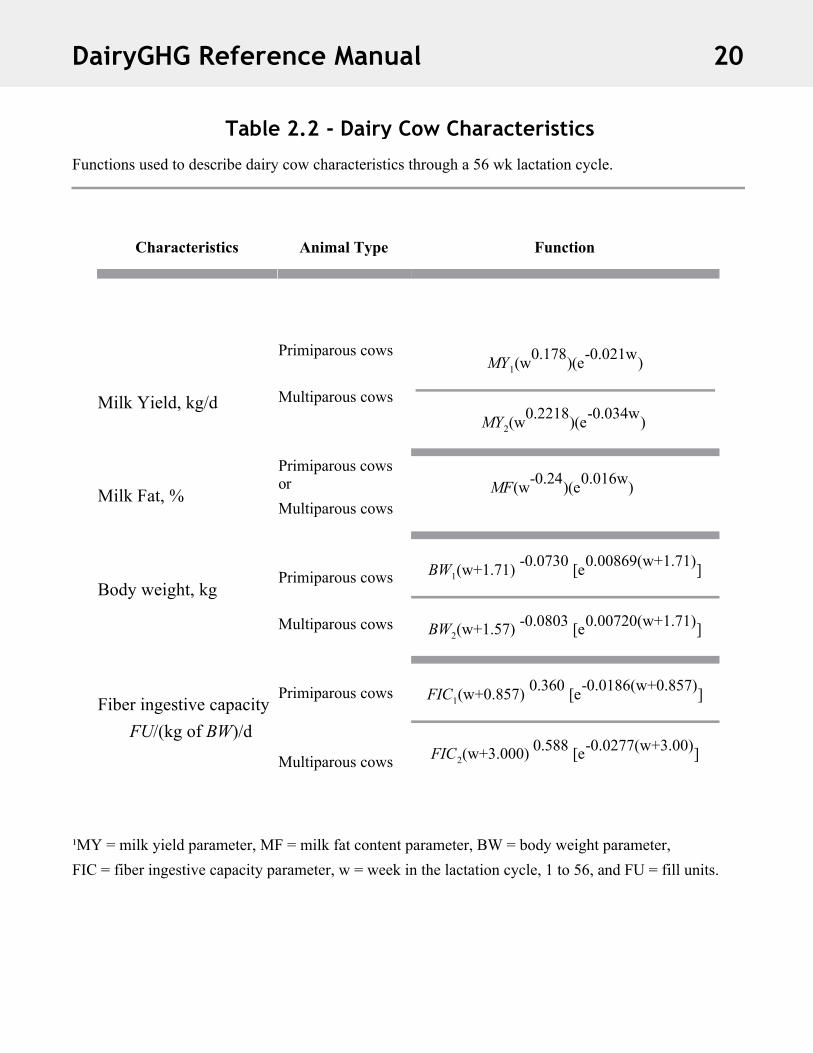
Functions used to describe dairy cow characteristics through a 56 wk lactation cycle.

¹MY = milk yield parameter, MF = milk fat content parameter, BW = body weight parameter,FIC = fiber ingestive capacity parameter, w = week in the lactation cycle, 1 to 56, and FU = fill units.

Table 2.2 - Dairy Cow Characteristics

Characteristics Animal Type Function

Milk Yield, kg/d

Milk Fat, %

Body weight, kg

Fiber ingestive capacity FU/(kg of BW)/d

Primiparous cows

Multiparous cows

Primiparous cows orMultiparous cows

Primiparous cows

Multiparous cows

Primiparous cows

Multiparous cows

MY1(w0.178)(e-0.021w)

MY2(w0.2218)(e-0.034w)

MF(w-0.24)(e0.016w)

BW1(w+1.71) -0.0730 [e0.00869(w+1.71)]

BW2(w+1.57) -0.0803 [e0.00720(w+1.71)]

FIC1(w+0.857) 0.360 [e-0.0186(w+0.857)]

FIC2(w+3.000) 0.588 [e-0.0277(w+3.00)]


Constraints and associated equations used to develop dairy animal rations.

ADIPi = acid detergent insoluble protein concentration in feed i (fraction of CP)

AMMj = adjustment factor for multiple of maintenance in lactating animal group j

AUPi = available RUP in feed i, fraction of DM

BWj = body weight of animal group j, kg

CPi = CP concentration in feed i, fraction of DM

RPDi = rumen degradability of protein in feed i, fraction of CP

DMI = DMI estimate which resolves NEm intake with NEm and NEg requirements, kg/d

Table 2.3 - Dairy Ration Constraints

Constraint Equations

Physical fillEffective fiberEnergy requirementRumen degradable proteinRumen undegradable protein

∑ xi (FUi )

∑ xi (RUi-0.21)

∑ xi (NEi)

∑ xi (CPi) (RPDi + 0.15)

∑ xi 0.87 (AUPi)

≤ FIC j (BWj)

≥ 0

= [NEDj + 0.7 (ECPj)] AMMj

≥MCPi / 0.9

≥MPRj - 0.64 (MCPi)

Associated Equations

Adjustment for multiple of maintenance

Available undegraded protein

Microbial crude protein

Excess protein

AMMj = 0.92 / [1-0.04 (NER j / NEMj - 1)

AUPi =CPi [1-RPDi - UFi (ADIPi)]

MCPj = 0.13 (TDNDj)(DMIj)

ECPj = ∑ xi (CPi) [RPDi + 0.15 + 0.87 (1 - RPDi - UFi (ADIPi)]- 0.7 MPRj + 0.47 (MCPj)]


ECPj = excess protein consumption, kg/d

FICj = fiber ingestive capacity, kg NDF/kg SBW/d

FUi = fill units (NDF adjusted for particle size and digestibility; Rotz et al., 1999a) of feed i, fraction of DMMCPj = microbial crude protein production in animal group j, kg/d

MPRj = metabolizable protein requirement of animal group j, kg/d

NEi = NEm concentration in feed i, MCal/kg DM

NEMD = diet NEm which resolves NEm intake with NEm and NEg requirements, MCal/kg DMNEMj = net energy requirement for maintenance of animal group j, MCal

NERj = net energy requirement of animal group j, MCal

RUi = roughage units (NDF adjusted for particle size and digestibility; Rotz et al., 1999a) of feed i, fraction of DMTDNDj = total digestible nutrient concentration of the diet, fraction of DM

UFi = unavailable fraction of ADIP (0.7 for forages and 0.4 for concentrates).

xi = amount of feed i in the diet, kg DM/d

1∑ means the summation over all feeds in the ration


The manure component simulates a variety of options in manure handling including methods of manure collection, storage, transport, and application. Collection methods include hand scraping or gutter cleaner, an alley scraper or tractor mounted scraper, and a flush system. Storage methods include a cement pad and buck wall for short-term storage of semi-solid material and tanks or earthen retention ponds for slurry or liquid manure storage. Transport and application is done with spreaders or irrigation equipment with manure spread on field surfaces, injected into the soil, or irrigated. All N flows through the dairy herd are tracked to determine a nutrient balance. Nitrogen intake is that consumed in feeds. Nutrient levels in feeds are set by the user where N concentration is protein content divided by 6.25. Nutrient outputs include milk, animal tissue, and manure. Nutrient levels in milk and animal tissue are those given above in the Dairy Herd section above. The efficiency of N use is the N obtained in milk and animal tissue divided by the total consumed in feed.

The quantity and nutrient content of the manure produced by the animals on the farm is a function of the feeds fed as described in the Dairy Herd section above. The total quantity of manure handled is a function of the amount and type of bedding used and the amount of water contained in the manure. Bedding options include straw, sawdust, and sand with the bedding type selected by the user. The user also sets the amount of bedding used per mature animal in the herd. The quantity of bedding used is determined by calculating the number of animal units on the farm with the mass of an animal unit being the average mass of a mature cow in the herd. This animal mass varies with the animal breed selected. The number of animal units thus reflects the total animal mass on the farm (including young stock) expressed in units of mature animals. Bedding use is the product of mature animal units and the use per animal unit. The quantity of wet manure handled is determined from total manure DM and the user selected manure type. Manure types are solid, semisolid, slurry, and liquid. Total manure handled is the total manure DM divided by the DM content plus DM from bedding and feed lost into the manure. Although manure DM contents can be adjusted, preset values are 20, 13, 8, and 5% for solid, semisolid, slurry, and liquid manures. Solid manure reflects that from packed beds, and semi-solid represents fresh manure plus bedding. Slurry manure typically includes milking facility wastewater and additional water from rain runoff from animal holding areas. For liquid manure, additional water from rain or other sources such as flush water is assumed and a liquid/solid separator may be used.

Storage Manure storage options include long-term storage in tanks or clay- or plastic-lined earthen retention ponds. Essentially any storage size can be selected by setting an average diameter and depth for the structure. The type and size of storage selected controls the amount of manure that can be stored, and it influences the amount of volatile loss that occurs from storage. Storage options include short-term, four-month, six-month, and twelve-month storages. With short-term storage, manure must be hauled each day. This option can also be used to represent short-term storage on a slab or in a small pit. With a four-month storage, manure is emptied three times each year in the spring, summer, and fall. With a six-month storage, manure is emptied twice each year in the spring

MANURE AND NUTRIENTS

Manure Handling


and fall. For twelve-month storage, it is emptied once a year in the spring. For either of the two long-term storage options, the manure produced during that period of time each year is compared to the storage capacity. If the storage is too small to hold the manure produced, the simulation continues but a warning message is given that the user should consider increasing the storage size. When stored in a concrete or steel tank, manure can be added to the top or bottom of the tank. Top loading represents scraping or pumping of the manure onto the top surface; whereas, bottom loading represents the pumping of manure into the bottom. With bottom loading, a crust can form on the manure surface. This crust helps seal the surface, reducing volatile loss from the storage facility. Covered or enclosed tanks can also be used for manure storage to reduce volatile losses. A covered storage is defined to have some type of cover that is relatively effective in preventing volatile loss. An enclosed tank is more effective with a sealed top that is vented to prevent pressure buildup within the tank. Thus, volatile emissions are minimal with an enclosed top, but small amounts still escape through the vent. A flare is used to burn the escaping biogas to reduce methane emission.

Application Manure deposited during grazing is applied to the grazed crop, and this portion is not included in the value for total manure handled, i.e. the manure handled is the total produced minus that deposited during grazing. The amount applied during grazing is proportional to the time the animals spend in the pasture. When animals are maintained on pasture year around, about 85% of the total manure produced is deposited during grazing. For seasonal grazing, this value is about 40%. Manure application is simulated on a daily time step. For daily hauling (or short-term storage) of manure, hauling and application occur each day with that applied being that produced on the given day. When a storage facility is emptied, manure is applied each day suitable for field operations until the storage is emptied. The amount applied each day is the total manure accumulated during the storage period divided by the days available for field application.

Manure can be brought into the production system or exported to another use. This affects the nutrient balance of the farm and the predicted emissions. When manure is imported, the farm owner provides a service to the manure producer by supplying land for disposal of the manure. The farm can also obtain benefit from the use of the added nutrients. Any emissions following land application are attributed to the production system receiving the manure.

When fresh manure or separated manure solids are exported, that portion of the nutrients are removed from the production system and any emissions following land application are not attributed to the farm. When manure is exported in the form of compost, that portion of the nutrients are again removed, but emissions during composting are attributed to the farm. Nutrient Import

When manure is carried onto the farm, the amount of manure imported and the dry matter and nutrient contents of that manure are provided by the model user. The amount of manure dry matter applied to cropland is the sum of that produced on the farm and that imported. Likewise, the total quantity of N is the sum of that produced and that imported.

Manure Import and Export


The flow, transformation, and loss of the added manure nutrients follows the same relationships used for the farm-produced manure. The manure carried onto the farm has volatile losses following field application, but losses that occur in the barn or during storage and handling are not included. These losses have occurred before the manure is brought onto the farm, which should be considered when setting the N content of the imported manure. The N volatilization rate following field application is set at the same rate as that for manure produced on the farm. This is a function of the volatile (ammonium) N content of the manure and the time between spreading and incorporation of the manure. The fraction of N that is in a volatile form is set to be the same as that produced on the farm. If no manure is produced on the farm, the volatile N content of the manure is set at 40% of the total N in the imported manure.

Nutrient Export Manure nutrients can leave the farm as fresh manure, separated solids, or compost. Similar but somewhat different relationships are used to model the effect of each type of export. The manure dry matter exported is set as a portion of the total manure dry matter produced on the farm. This can be anywhere from 0 to 100% of the manure solids produced.

When the export is fresh manure, the nutrients removed are the nutrient contents of the manure following storage (or following barn scraping if no storage exists) times the manure dry matter removed from the farm. The N content is that determined after volatile losses occur in the barn and during storage (if manure storage is used). For the portion of the manure exported from the farm, the N loss that would have occurred following land application are eliminated.

When separated manure solids are removed from the farm, the nutrient removal is the dry matter removed times the nutrient contents of the removed solids. By default in the program, the N, P, and Kcontents in organic bedding material (straw or sawdust) are set at 1.4, 0.3, and 0.4%, respectively (Chastain et al., 2001; Meyer, 1997). With sand bedding, fewer nutrients are retained in the solids, so the N, P, and K contents are set at 0.8, 0.15, and 0.4% respectively (Van Horn et al., 1991; Harrison, unpublished data). The nutrient contents of the removed solids can also be set in the farm parameter file. When values are set, the default values in the program are overwritten by the user specified values. The amount of manure handled and the nutrients in the remaining manure are adjusted for the solids removed. The solids removed are assumed to contain 40% DM. The manure applied to feed producing cropland is that produced minus the solids removed and the moisture contained in those solids. The DM content of the remaining manure is the original DM minus that exported divided by the remaining quantity of manure. Nutrients remaining in the production system following separation are those in manure received from the barn minus that leaving in separated solids. Nutrient losses during storage and following land application are reduced in proportion to the amount removed. The remaining option is to remove manure and nutrients in the form of compost. The manure removed as compost reduces the amount of manure stored and applied to cropland. When a portion of the manure is exported as compost, the nutrient content of the manure removed is that following barn scraping. The portion removed reduces N losses during storage and field application in proportion to that removed. There are N losses during the composting process, which are included as loss from the farm. The portion of the N lost by volatilization during composting is assumed to be the volatile N content in the manure following scraping plus 25% of the organic N content (Sommer, 2001; Ott et al., 1983). This N loss is added to that that occurs during the storage of farm-produced manure increasing the total volatile N loss from the farm.


Simulated greenhouse gas emissions include CO2, CH4, and N2O. A major CO2 sink occurs through the fixation of carbon in crop growth with emission sources including plant respiration, animal respiration, and microbial respiration in the soil and manure. Major sources of methane include enteric fermentation and long term storage of manure with minor sources being the barn floor, field applied manure, and feces deposited by grazing animals. Nitrous oxide is a product of nitrification and denitrification processes in the soil and these processes can also occur in the crust on a slurry manure storage or during the storage of solid manure in a bedded pack or stack. A comprehensive evaluation of production systems is obtained by considering the integrated effect of all sources and sinks of the three gases.

Multiple processes emit CO2 from dairy farms. The major source is animal respiration, followed by less significant emissions from manure storages and barn floors. Cropland assimilates CO2 from the atmosphere through fixation during crop growth and emits CO2 through plant and soil respiration. Typically, over the course of a full year, croplands assimilate C from CO2. In other words, the plants capture more CO2 through photosynthesis than is emitted through respiration. Cropland Emissions A relatively simple but robust approach is used to predict net CO2 emission from feed production in cropland. The long term carbon balance for the cropland producing feeds is assumed to be zero. Therefore, the sum of all carbon leaving the cropping system in feed and emissions is equal to that assimilated during the growth of the crop (i.e., the capture of CO2 through photosynthesis) plus any other C entering the cropping system. Emissions of CO2 from cropland include that from plant respiration (autotrophic) and soil respiration (heterotrophic), as well as microbial respiration during the decomposition of manure. The primary source of non photosynthetic C entering the system is land applied manure. A carbon balance is determined considering all flows in and out of cropland during the production of feeds used in the dairy production system. By enforcing a long term balance, the net difference between that fixed during crop growth and that emitted through plant and soil respiration must equal the C removed in harvested feed minus that applied to the cropland in manure. Applied manure is that excreted by the animals minus all C lost in the barn, during manure storage, and following land application plus any C in manure imported to the farm and minus that exported from feed production. Therefore, the net flux of C in feed production is determined as: Cnet = Cfeed – (Cexc – CCH4 – CCO2 – Cexp + Cimp) [4.1] where Cnet = net flux of C assimilated in feed production minus plant and soil respiration, kg Cfeed = C in feed produced plus that in bedding minus that in excess feed, kg Cexc = C in manure excreted by animals on the farm, kg

GREENHOUSE GAS EMISSIONS

Carbon Dioxide


CCH4 = C lost as CH4 from barn floor, during storage, and following land application, kg CCO2 = C lost as CO2 from the barn floor and manure storage, kg Cexp = C in manure exported from feed production, kg Cimp = C in manure imported to farm, kg The C content of most feeds is set at 40% of DM, but that in high protein concentrates is set at 45% of DM and that in added fat is set at 70%. The C in manure excreted by the animals is determined using a C balance of the herd where the C intake must equal the C output. Therefore, the C excreted is equal to that consumed in feed minus that emitted by the animals in CH4 and CO2 and that contained in the milk and animal weight produced. Carbon in exported manure is determined as the user-defined portion of manure exported times the C remaining in excreted manure after storage. Imported manure is assumed to have a C content of 40% of DM. Emissions of CH4 and CO2 are as defined in the following sections. Since the net flux of C in feed production, Cnet, represents a net exchange of CO2 with the atmosphere, it can be converted to units of CO2. A conversion is done by multiplying the units of C by

the ratio of the molecular weight of CO2 (44 g mol-1) to that of C (12 g mol-1). Therefore, there are 3.67 kg of CO2 assimilated or released per kg of C. It is important to note that this approach does not allow for long term sequestration or depletion of soil C. By forcing a long term balance, it is assumed that there is no net change in soil C content over time. If major changes in tillage and cropping practices are made, soil C levels can change over a number of years until the soil again reaches an equilibrium level. An example of this type of change is the conversion of row cropland to perennial pasture. Substantial amounts of soil C can be sequestered over 25 to 50 years until equilibrium soil conditions are maintained. Another example is the conversion of conventional tillage to reduced tillage or no tillage practices. Such conversions can increase the net flux of C into feed production, i.e. reduce net CO2 emission. Our model does not account for this potential change in soil C, but this change can be added or subtracted from the net value determined by DairyGHG. To obtain values for quantifying long term changes in soil C, we recommend the COMET-VR model available at http://www.cometvr.colostate.edu/tool/default.asp?action=1. COMET-VR provides a relatively easy to use tool for quantifying potential changes in soil C with changes in production practices. Values obtained can be used to adjust values predicted by DairyGHG.

Animal Respiration Carbon dioxide emission through animal respiration is sometimes ignored as a GHG emission source (IPCC, 2001 and 2007). This respired CO2 is part of the C cycle that initially begins with photosynthetic fixation by plants. When the animals consume the crop (fixed C in the plant material), they convert it back to CO2 through respiration (Kirchgessner et al., 1991; IPCC, 2001). On a farm, animal respiration of CO2 is a major source relative to other CO2 emissions. In the overall farm balance, the CO2 released largely offsets the CO2 assimilated in the plant material. However, some of the feed intake of C is converted and released as CH4 and some is in the milk and animals produced. To obtain a full accounting and balance of all C flows through the farm, all sources of C emissions, including animal


respiration, are considered.

A relationship developed by Kirchgessner et al. (1991) relating CO2 emissions to DMI is used to predict animal respiration. Respired CO2 is determined as:

ECO2,resp = -1.4 + 0.42 · MDMI + 0.045 · MBW0.75 [4.2]

where ECO2,resp = emission of CO2 from animal respiration, kg CO2 head-1 day-1

MDMI = daily intake of feed dry matter for each animal, kg DM head-1 day-1

MBW = animal body weight, kg. The DMI and body weight for each animal group are available from the herd component. Dry matter intake is determined based upon the nutrient requirements (fiber, energy and protein) of a representative animal for each group within the herd and the amount and nutrient content of available feeds including pasture (See Dairy Herd section). Body weight is determined based upon animal breed, as specified by the model user, and the age and stage of lactation as simulated in the herd component.

Barn Floor Emissions Floors of housing facilities can be a source of CO2 emissions due to decomposition of organic matter in manure deposited by animals. Although not a major source, barn floor emissions are included to obtain a comprehensive simulation of farm-level CO2 emissions from all sources.

Published models to predict CO2 emissions from barn floors were not found. Using emissions data measured from manure covered floors in a free stall barn at the Penn State dairy facility (Wheeler et al., 2008), an equation was developed through regression analysis relating CO2 emission to the

ambient temperature in the barn and the manure covered floor area (R2 = 0.74).

ECO2,floor = max (0.0, 0.0065 + 0.0192 T ) Abarn [4.3]

where ECO2,floor = daily rate of CO2 emission from the barn floor, kg CO2 day-1

T = ambient temperature in the barn, °C Abarn = floor area covered by manure, m2

Equation 4.3 represents the best available information describing CO2 emissions from barn floors. As a function of temperature, this relationship provides a simple process-based model that predicts reasonable emission rates over a full range in potential ambient barn temperatures. Because barn floor emissions are so small compared to other sources, development of a more sophisticated model was not justified at this time. Manure Storage Compared to other farm sources, slurry storages emit relatively low amounts of CO2. Because of this minimal contribution to whole-farm emissions, there were no models and few data available


quantifying CO2 emissions from storages. Lack of available data, as well as the relative importance of this loss to overall farm emissions did not support the development of a detailed model. Therefore, a constant emission factor represented the best available method for predicting this emission. To determine an emission factor, emission rates were obtained from two published studies and the average was used as our emission rate (Table 4.1).

The average emission rate of 0.04 kg CO2 m-3 day-1 is applicable to uncovered slurry storages. Covers are sometimes used to reduce gaseous emissions, but no data were available documenting the effect of covers on CO2 emissions. To model this effect, we assumed that CO2 emissions are reduced by a similar proportion when using a cover as found for more important gases such as ammonia. For ammonia, a cover reduces emission by about 80%, depending upon the storage dimensions (Rotz et al., 2008). Therefore, to simulate CO2 emissions from a covered storage, the emission rate was reduced to

0.008 kg CO2 m-3 day-1. To represent a sealed storage where biogas is burned, the loss of CO2 was eliminated. However, the total emission from this type of storage includes the CO2 created through the combustion of CH4. (see the following section on CH4 emission). Engine Combustion During the operation of tractors and other engine powered equipment, C in fuel is transformed to CO2, which is released in engine exhaust. The amount of CO2 produced is proportional to the amount of fuel consumed. The emission factor used is 2.637 kg CO2e/liter of diesel fuel consumed (Wang, 2007).

Fuel consumed in the production system is estimated through the use of fuel use factors. These factors represent a typical or average amount of fuel used to produce and deliver a unit of feed to the herd or remove a unit of manure. Fuel use factors were determined with the use of the Integrated Farm System Model (Rotz et al., 2008). This farm model simulates feed production and use over many years of weather. By simulating various feed production systems, average amounts of fuel use per unit of feed produced and fed were determined for each of the major types of feed used in dairy production (Table 4.5). This same approach was used to determine a factor for manure handling of 0.6 liter/t of manure removed from the barn. By summing the products of the fuel use factors and the amount of each feed used or the amount of manure handled, an estimate of total fuel use is obtained. Fuel use is then multiplied by the emission factor to obtain engine CO2 emissions.

Methane is a strong GHG with a GWP around 25 times that of CO2 (IPCC, 2007). Multiple processes emit CH4 from dairy farms. The majority of CH4 is created through enteric fermentation, followed by emissions from manure storages (EIA, 2006; Chianese et al., 2009). In addition to these major sources, smaller emissions result from field-applied manure and manure deposited by animals inside barns or on pasture. Most field studies report croplands as a negligible source, or very small sink, of CH4 over full production years. However, field-applied manure can result in significant emissions for a few days after application. In DairyGHG, emissions from cropland are neglected except for this small emission that occurs immediately after manure application.

Methane Emission


Enteric Fermentation Ruminant animals subsist primarily on forages. Like most animals, ruminants do not have the enzymes necessary to break down cellulose. Instead, enteric methanogens, which exist in a symbiotic relationship with other microorganisms in the rumen, break down and obtain energy from cellulose. During this process, hydrogen is produced and can build up in the rumen, leading to acidosis, a health problem in dairy cows. However, these methanogens decrease the amount of hydrogen in the rumen by using the excess to reduce CO2 to CH4, preventing this health effect. The CH4 produced is released to the atmosphere by eructation and respiration. The amount of CH4 produced from enteric fermentation is impacted by various factors including animal type and size, digestibility of the feed, and the intake of dry matter, total carbohydrates, and digestible carbohydrates (Monteny et al., 2001; Wilkerson et al., 1995). After considering the various mechanistic and empirical models available to predict enteric fermentation emissions (Wilkerson et al., 1995; Benchaar et al., 1998; and Mills et al., 2003), a relatively simple approach is used, which uses the Mitscherlich 3 (Mits3) equation developed by Mills et al. (2003). Mits3 is a simplified process model that is well suited for use in whole-farm simulation. The model is based on dietary composition and is capable of accounting for management practices that alter the animal’s intake and diet. Mits3 is process-based, relating CH4 emissions to dietary intake as well as animal type and size. When compared to data from the U.S., Mits3 has yielded a regression slope of 0.89 with an intercept of 3.5 and a square root of the mean square prediction error (MSPE) of 34% (Mills et al., 2003). In addition, Mits3 predicts realistic emissions at the extremes of the parameter ranges. With zero feed intake, the model predicts zero CH4 production; at the other extreme of very high feed intake, the nonlinear model predicts that CH4 emission approaches a maximum. Thus, the model can be applied to conditions outside those for which it was originally developed without predicting unreasonable emissions. Three model inputs are required: starch content of the diet, acid detergent fiber (ADF) content of the diet, and metabolizable energy intake. These inputs are readily obtained from the feed and animal components of DairyGHG. Through these inputs, CH4 production is directly related to diet and indirectly related to animal size and type. This allows prediction of changes in CH4 production as affected by changes in animal nutrition and management. A detailed description of the selected model can be found in Mills et al. (2003).

Enteric emission of CH4 is predicted as: ECH4,ent = [ Emax - Emax exp(-c · MEI ) ] FkgCH4 [4.4]

where ECH4,ent = emission due to enteric fermentation, kg CH4 head-1 day-1

Emax = maximum possible emission, MJ CH4 head-1 day-1

c = shape parameter for how emissions change with increasing MEI, dimensionless

MEI = metabolizable energy intake, MJ head-1 day-1

FkgCH4 = conversion of MJ to kg of CH4, 0.018 kg CH4 MJ-1


From Mills et al. (2003), the maximum possible emission is defined as 45.98 MJ CH4 head-1 day-1. This maximum possible emission is constant for all animals; the effect of animal size and type is indirectly provided through the value of MEI. The shape parameter, c, is calculated as: c = -0.0011· [Starch / ADF] + 0.0045 [4.5] where Starch = starch content of the diet, fraction ADF = acid detergent fiber content of the diet, fraction Equation 4.4 models the observed trend of increased CH4 emission with high fiber diets and decreased emission with high starch diets. To use the above equations, values are needed for the starch and ADF contents of diets and the metabolizable energy intake of animal groups making up the herd. The herd component determines the ration that each animal group is fed based upon a representative animal’s nutritional requirements and the available feeds (See Herd and Feed Sections). This information includes the required energy content of the diet [MJ kg DM-1], the total dry matter intake [kg DM day-1 head-1], and the amount of each feed used. The first two parameters are used to calculate MEI. The ADF contents of feeds are determined assuming a linear relationship with neutral detergent fiber (NDF) for each feed type (Table 4.2). These relationships were developed using feed composition data from the National Research Council (NRC, 2001). The starch contents of feeds are determined assuming a linear relationship with the amount of non fiber carbohydrate (NFC) in the feed (Table 4.2). The fraction of NFC is determined as:

FNFC = 1 - (FNDF + FCP + Ffat + Fash ) [4.6] where FNFC = fraction of NFC in the diet FCP = fraction of crude protein (CP) in the diet Ffat = fraction of fat in the diet Fash = fraction of ash in the diet. The fractions of NDF and CP are available in the herd component; typical fractions of fat and ash (Table 4.2) were obtained from the National Research Council (NRC, 2001). A given animal group is typically fed a mixture of feeds making up the whole diet. A weighted average of the individual feed characteristics in the ration is used to determine the starch and ADF contents of the full ration fed to each of the six possible animal groups making up the herd.

Barn Emissions Manure on housing facility floors is also a small source of CH4. No published model or data were found for this emission source. Therefore, unpublished CH4 emission data measured from free stall barn floors (Wheeler et al., 2008) were used to develop an empirical equation relating CH4 emission to

the ambient temperature in the barn (R2 = 0.48). The resulting model is:

ECH4,floor = max(0.0, 0.13 T ) · Abarn / 1000 [4.7]


where ECH4,floor = daily rate of CH4 emission from the barn floor, kg CH4 day-1

T = ambient barn temperature, °C Abarn = area of the barn floor covered with manure, m2

This relationship represents the best available information describing CH4 emissions from free stall and tie stall barn floors. The temperature dependence of CH4 production is well-documented (Zeikus and Winfrey, 1976; van Hulzen et al., 1999). This simple relationship predicts reasonable emission rates for ambient temperatures of 0°C and greater. When manure is allowed to accumulate into a bedded pack, CH4 emissions are increased. For this management option, an adaptation of the tier 2 approach of the IPCC (2006) is used. Emission on a given day is determined as a function of the ambient barn temperature and a methane conversion factor (MCF).

ECH4,floor = VS (Bo) (0.67) (MCF) / 100 [4.8]

where ECH4,floor = daily CH4 emission, kg CH4 day-1

VS = volatile solids excreted in manure, kg VS Bo = maximum CH4 producing capacity for dairy manure, 0.24 m3 CH4 (kg VS)-1

0.67 = conversion factor of m3 CH4 to kg CH4 MCF = CH4 conversion factor for the manure management system, %. MCF is modeled as an exponential function of ambient barn temperature through a regression of the data provided by the IPCC (2006):

MCF = 7.11 e 0.0884(Tb) [4.9]

where Tb = ambient barn temperature, oCMCF is limited to a minimum value of 0 and maximum of 80. In warm dry climates, animals are often housed in open, non vegetated areas normally referred to as drylots. Manure typically accumulates on the soil surface for weeks or months before being removed. To predict emissions from this surface, the tier 2 approach of IPCC (2006) is again used. Based upon the IPCC (2006) data, MCF was modeled as a linear relationship with ambient outdoor temperature: MCF = 0.0625 Ta – 0.25 [4.10]

whereTa = ambient temperature, oC.MCF is limited to a minimum value of 0. In systems that combine free stall and drylot housing, the assumption is made that half of the manure is deposited in free stall allies with the remainder deposited on the drylot. The total emission is then the sum of the two sources modeled using the appropriate relationships.


Manure Storage During manure storage, CH4 is generated through a reaction similar to that described for enteric fermentation. The cellulose in the manure is degraded by microbes, with products of this process serving as substrates for methanogenesis. Temperature and storage time are the most important factors influencing CH4 emissions from stored manure because substrate and microbial growth are generally not limited (Monteny et al., 2001). Although the processes are similar, there are important differences between the rumen and manure storage. The temperature in the storage varies, in contrast to the relatively constant temperature in the rumen, and the manure in storage is more heterogeneous (e.g., the substrate is less well mixed and some carbohydrates are already partially decomposed) as compared to the consistency of the rumen (Monteny et al., 2001). As with enteric fermentation, both mechanistic and empirical models have been developed to predict CH4 emissions from manure storages. Unlike some of the empirical enteric fermentation models that simply use statistical correlations, the majority of empirical manure storage models are biologically based. After considering two mechanistic (Hill, 1982; and García-Ochoa et al., 1999) and four empirical models (Chen and Hashimoto, 1980; Hill, 1991; Zeeman, 1994; and Sommer et al., 2004), the model of Sommer et al. (2004) was selected as the most appropriate approach for our application. Their model employs commonly used empirical relationships (e.g., Arrhenius relationship) that are more general and thus more applicable to conditions outside of which they were developed. Additionally, this is a more recent model, incorporating more recent developments and data. Unlike most the other models, the model of Sommer et al. (2004) was developed for more general application to either digested or untreated slurry manure. The model of Sommer et al. (2004) simulates the production and emission of CH4 from manure storages based upon the degradation of volatile solids (VS). Additional factors affecting CH4 production are temperature and storage time. A detailed description of the development of their model is found in Sommer et al. (2004). Emission of CH4 from manure storage is predicted as:

ECH4,man = (( 24·Vs,d · b1)/1000)·exp[ln(A) - (E/RT)]+

((24·Vs,nd ·b2)/1000)·exp[ln(A) - (E/RT)] [4.11]

where ECH4,man = emission of CH4 from the storage, kg CH4 day-1

Vs,d and Vs,nd = degradable and nondegradable VS in the manure, g b1 and b2 = rate correcting factors, dimensionless

A = Arrhenius parameter, g CH4 kg-1 VS h-1

E = apparent activation energy, J mol-1

R = gas constant, J K-1 mol-1

T = temperature, oK (Table 2). From Sommer et al. (2004), the degradable volatile solids entering storage is:


Vs,d = Vs,tot [ Bo / ECH4,pot ] [4.12] where Vs,tot = total VS in the manure, g

Bo = achievable emission of CH4 during anaerobic digestion, g kg-1 VS

ECH4,pot = potential CH4 yield of the manure, g (kg VS)-1

ECH4,pot can be estimated using Bushwell’s equation and the carbohydrate, fat, and protein content of

the manure. For cattle slurry, Sommer et al. (2004) defined Bo as 0.2 g CH4 (kg VS)-1 and ECH4,pot as

0.48 g CH4 (kg VS)-1. Total VS in the manure storage at any point in time is the difference between that entering the storage and that lost from the storage up to that point. The amount entering is determined from the manure mass removed from the barn, the total solids content, and the VS content:

Vs,tot = Mmanure · PTS · PVS - Vs,loss [4.13]

where Mmanure = accumulated mass of manure entering the storage, kg

PTS = total solids content in the manure, g TS (kg manure)-1

PVS = fraction of VS in the total solids, g VS (g TS)-1

Vs,loss = accumulated VS loss. To obtain a similar rate of VS loss as that reported by Sommer et al. (2004), this loss was predicted as three times the methane loss from the stored manure. The mass of nondegradable volatile solids, Vs,nd, is then calculated using a mass balance:

Vs,nd = Vs,tot - Vs,d [4.14]

The inputs required are the mass and temperature of the manure in storage. The amount of manure in storage is modeled as the accumulation of that produced by the herd while in the barn with daily manure excretion determined in the animal component (See Manure DM and Nutrient Production section). The temperature of the manure in storage on a given simulated day is estimated as the average ambient air temperature over the previous ten days (Table 4.3). This predicted storage emission is for an uncovered, bottom-loaded storage of slurry (7 – 12% DM) manure where a crust forms on the surface. For a top-loaded tank or with manure containing less DM, this emission rate is increased 40% (IPCC, 2006). Storage covers are sometimes used to reduce emissions. With a non-sealed cover, the emission rate is reduced to 20% of that occurring from the open storage. A more tightly sealed cover or enclosed storage can be used where the biogas produced is burned to convert the emitted CH4 to CO2. This technique drastically decreases the emission of CH4, although it does increase the emission of CO2 through the combustion of CH4. To simulate this storage treatment, the emission of CH4 from an enclosed manure storage is calculated as:


ECH4,cov = ECH4,man · (1-ηeff ) [4.15]

where ECH4,cov = CH4 emitted from the enclosed manure storage, kg CH4 day-1

ECH4,man = CH4 emission from the storage with no cover using equation 4.11, kg CH4 day-1

ηeff = efficiency of the collector, dimensionless The efficiency of the collector and flare is assumed to be 99% (EPA, 1999). The subsequent flaring of the captured CH4 releases CO2, which adds to the overall farm emission of this gas. Assuming complete combustion, the additional emission of CO2 due to the combustion of CH4 is calculated as:

ECO2,flare = ECH4,cov · 2.75 [4.16]

where ECO2,flare = emission of CO2 from the combustion of captured CH4, kg CO2 day-1

2.75 = ratio of the molecular weights of CO2 and CH4. Semi-solid (8-14% DM) and solid manure (>15% DM) can be stored in stacks. Methane emission from this type of storage is modeled through an adaptation of the tier 2 approach developed by the IPCC (2006). Emission on a given day is determined as a function of the total volatile solids (VS) placed into the storage and the methane conversion factor:

ECH4 = VS (Bo) (0.67) (MCF) / 100 [4.17]

where ECH4 = daily CH4 emission, kg CH4 day-1

Bo = maximum CH4 producing capacity for dairy manure, 0.24 m3 CH4 (kg VS)-1

0.67 = conversion factor of m3 CH4 to kg CH4 MCF = CH4 conversion factor for the manure management system, %. Using the recommended data of the IPCC (2006), a function was developed to predict MCF as a function of the temperature of the stored manure: MCF = 0.201 Tm – 0.29 [4.18]

where Tm = manure temperature, oC. MCF is set at a minimum of zero, and the manure temperature is the average ambient temperature over the previous 10 days. Field-Applied Manure Research has shown that field-applied slurry is a source of CH4 for several days after application,

emitting between 40 to 90 g CH4 ha-1 day-1 (Sommer et al., 1996; Chadwick and Pain, 1997; Sherlock et al., 2002). Emissions drastically decrease within the first few days, and the soils return to a neutral source of CH4 by 11 days (Sherlock et al., 2002).


Sherlock et al. (2002) related CH4 emissions from field-applied slurry to the volatile fatty acids (VFAs) concentration in the soil. Because the VFAs in the soil are due to the application of the slurry (Sherlock et al., 2002), their model is used to relate CH4 emissions to the VFA concentration in the slurry. Emission of CH4 from field-applied slurry is predicted as: ECH4,app = (0.170 · FVFA + 0.026 ) · 0.032 · Aman / rapp [4.19]

where ECH4,app = emission of CH4 from field-applied slurry, kg CH4 day-1

FVFA = daily concentration of VFAs in the slurry, mmol (kg slurry)-1

Aman = amount of manure applied, kg

rapp = application rate, kg ha-1

Sherlock et al. (2002) found that the daily VFA concentration exponentially decreased in the days following the application of manure slurry and approached background levels within approximately four days. Using this information, we derived a relationship predicting the daily concentration of VFA in the field-applied slurry:

FVFA = FVFA,init e-0.6939t [4.20]

where FVFA = daily concentration of VFAs in the slurry, mmol (kg slurry)-1

FVFA,init = initial VFA concentration in the slurry at application, mmol (kg slurry)-1

t = time since application with t = 0 representing the day of application, day Paul and Beauchamp (1989) developed an empirical model relating the pH of manure slurry to VFA and total ammoniacal nitrogen (TAN) concentrations: pH = 9.43 - 2.02 - [FVFA,init / FTAN ] [4.21] where pH = pH of the manure slurry, dimensionless FTAN = concentration of TAN (NH4

+ + NH3) in the slurry, mmol (kg slurry)-1

Rearranging Equation 4.21, we obtained an equation to predict the initial concentration of VFAs based on the pH and TAN of the manure slurry: FVFA,init = [FTAN / 2.02] (9.43 - pH) [4.22] To predict emissions from field applied manure, equation 4.22 was used to determine an initial VFA concentration and equation 4.20 was used to track the VFA concentration through time following field application. Using this concentration, an emission rate was determined until the remaining VFA concentration approached zero.


Grazing Animals On farms that incorporate grazing for at least a portion of the year, freshly excreted feces and urine are directly deposited by animals on pastures. Studies have shown that feces are a small source of CH4 and that emissions from urine are not significantly different from background soil emissions (e.g., Jarvis et al., 1995; Yamulki et al., 1999). Because animal-deposited feces contribute only minimally to overall farm CH4 emissions, there are few data quantifying these emissions. Due to the lack of supporting data and the relatively low importance of this emission source, a constant emission factor is used to predict CH4 from feces deposited by grazing animals. To determine this emission factor, emission rates were obtained from four published studies and the average (0.086 g CH4 (kg feces)-1) was used for our emission rate (Table 4.4). Therefore, for grazing systems, the daily emission of CH4 is predicted as the product of this emission rate and the daily amount of feces deposited by grazing animals.

Nitrous oxide is the strongest of all greenhouse gases emitted in agricultural production with a global warming potential 298 times that of CO2 (IPCC, 2007). In 2005, agriculture had the greatest overall impact on N2O emissions, contributing 78% of the U.S. total (EIA, 2006). In fact, this contribution has become increasingly important, with reported emissions increasing by 10% between 1990 and 2005 (EIA, 2006). Multiple sources emit N2O on dairy farms. The majority is emitted from soil, followed by manure storages, with relatively small amounts emitted from manure in bedded pack barns or drylots (Groenestein and Van Faasen, 1996; EPA, 2008).

Cropland Emissions Croplands are the largest source of N2O emitted from dairy farms. Although undisturbed soils emit N2O naturally, the rate of emission from cultivated soils is much greater because of the greater N inputs on farmland. Two pathways can lead to emissions of N2O: denitrification and nitrification. Denitrification is the microbial reduction of NO3 to N2 under anaerobic conditions, with the production of NO and N2O as intermediates (Figure 4.1).

Historically, denitrification was believed to be the primary source of N2O emissions; however, scientists have established that nitrification also contributes to emissions (Sahrawat and Keeney, 1986). Nitrification is an aerobic process that oxidizes NH4

+ to NO3, with the production of NO and N2O as intermediates (Figure 4.2).

The emission of N2O is thus dependent on both denitrification and nitrification. A conceptual model published by Davidson et al. (2000) describes how denitrification and nitrification are connected (Figure 4.3). This model, known as the “hole-in-the-pipe” (HIP) model, connects the two pathways and thus links the emission of NO and N2O (Davidson et al., 2000).

To simplify the model, soil processes are not simulated in DairyGHG. Therefore, a relatively

Nitrous Oxide


simple emission factor approach had to be used to estimate N2O emissions in the production of feeds. Based upon the recommendation of the IPCC (2007), the N2O-N emission from cropland is set at 1% of the N applied and that from pasture land is set at 2% of applied N. Since crop production is not simulated, N applied is set as 40% greater than that removed in harvested feed. This approach assumes relatively efficient use of N fertilizer in producing the feed crops. The over application of 40% allows for the loss of N that naturally occurs when N is applied at a recommended rate to meet nutrient removal. To predict N application, the total N in the feed consumed by the herd is determined as the sum of the DM for each feed consumed times the protein content divided by 6.25. This N is increased by 40% and multiplied by the appropriate emission factor and an N to N2O conversion factor of 1.57. The N deposited in pasture is proportioned by the time animals spend in the pasture, which is a function of the grazing system used. When animals are maintained outdoors all year, 85% of excreted N is applied to pastureland.

This approach was evaluated by comparing predicted emissions from this simple model to those predicted by a more complex process-based approach in the Integrated Farm System Model (Rotz et al., 2008). In general, average annual values predicted by the two approaches were similar even though this simple approach did not account for differences in soil type and climate conditions. Development of a more robust model for use in DairyGHG to predict N2O emission from cropland is planned.

Barn Emissions Manure on the floors of free stall and tie stall barns appears to be a negligible source of N2O emission. Based upon limited available data, the emission of N2O is modeled as zero from the floors of these facilities where manure is typically removed on a daily basis (Chianese et al., 2008d). For bedded pack and drylot surfaces where manure remains for longer periods, emissions can be greater. For these facilities, the IPCC (2006) tier 2 approach is used. Emission factors of 0.01 or 0.02 kg N2O-N (kg N

excreted)-1 are used for bedded pack and drylot facilities, respectively. The total N excreted in each facility is multiplied by the appropriate emission factor and the N to N2O conversion factor (1.57) to obtain N2O emission. For facilities that combine free stall and drylot use, half of the manure is assumed to be deposited in each.. Manure Storage Manure is stored as a liquid or in stacks. Nitrous oxide emission from slurry or liquid manure is predicted as a function of the exposed surface area of the manure storage and the presence of a crust on the surface. For an open slurry storage tank with a crust, an average emission rate of 0.8 g N2O m-2 day-

1 determined by Olesen et al. (2006) is used to predict N2O emissions:

EN2O,manure = EF,N2O,man · Astorage /1000 [4.23]

where EN2O,manure = emission of N2O from slurry storage, kg N2O day-1

EF,N2O,man = emission rate of N2O, 0.8 g N2O m-2 day-1

Astorage = exposed surface area of the manure storage, m2


This relatively simple model is justified given the lack of available information to support a more complex model and because the N2O emission from this type of manure storage is typically a relatively small portion of the whole farm emission of GHGs (Olesen et al., 2006).

The emission factor of 0.8 g N2O m-2 day-1 is applicable to bottom-loaded, uncovered slurry storage tanks where a natural crust forms on the manure surface. When a crust does not form on the stored slurry, no N2O is formed and emitted (Külling et al., 2003; Sneath et al., 2006). This occurs if the manure DM content is less than 8%, manure is loaded daily onto the top surface of the storage, or an enclosed tank is used. Therefore, when any of these manure handling options are selected, the emission rate is zero.

For stacked manure with a greater DM content, an emission factor of 0.005 kg N2O-N (kg N

excreted)-1 is used (IPCC, 2006). The excreted N stored in this manner is multiplied by this factor to predict a daily emission.

With the growing concern over global climate change and the potential impact of GHG emissions, a need has developed for expressing the total emission associated with a product or service. A term that has come to represent this quantification is the carbon footprint (http://en.wikipedia.org/wiki/Carbon_footprint). A carbon footprint is defined in many ways dependent upon the product or service represented. In general though, the carbon footprint is the total GHG emission, expressed in CO2 equivalent units (CO2e), associated with that product or service. The conversion to CO2e is done using the GWP of each gas where GWP values used for CH4 and N2O are 25 and 298, respectively (IPCC, 2001; EPA, 2007).

We define the carbon footprint of milk production to be the net of all greenhouse gases assimilated and emitted in the production system divided by the total energy corrected milk produced. This net emission is determined through a partial life cycle assessment of the production system (Figure 1.1). Emissions of CH4 and N2O are converted to CO2e units by multiplying by their GWP index. All emission sources of the three gases are summed and the net CO2 assimilated in feed production is subtracted to give the net emission of the production system. Emissions include both primary and secondary sources. Primary emissions are those emitted from the farm or production system during the production process. Secondary emissions are those that occur during the manufacture or production of resources used in the production system (machinery, fuel, fertilizer, etc.). Secondary emissions such as those in the manufacture of equipment must be apportioned to average annual values. By totaling the net of all annual emissions from both primary and secondary sources and dividing by the annual energy corrected milk production, a carbon footprint is determined in units of CO2e per unit of milk produced. The carbon footprint is primarily determined as the net emission of the three GHGs including all sources and sinks of CO2. A carbon balance is enforced, so a portion of the CO2 assimilated in the feed is in the carbon exported from the system in the milk and animals produced. Although this provides a more complete assessment of the carbon footprint of the production system, this procedure deviates from the more standard protocol followed by the IPCC and most other studies publishing carbon footprints of

Carbon Footprint


milk production. The more standard protocol does not consider assimilated CO2 and includes only the CO2 emitted by the combustion of fossil fuels. For comparison, a carbon footprint is also determined following this procedure. A minor deviation is included though to provide a more equitable assessment. The carbon in the CH4 emitted from the system comes from CO2 assimilated in feed. Therefore, the net GHG emission is reduced by the amount of CO2 assimilated to meet the CH4 emission. Including this refinement reduces the carbon footprint of the production system 8-10% depending upon the production strategy used. Use of this protocol increases the footprint about 30% compared to the first approach, which includes the CO2 assimilated in the carbon exported from the production system. Primary Sources Primary sources of GHG emissions include the net emission of CO2 plus all emissions of CH4and N2O occurring from the farm production system. Daily emission values of each gas are summed to obtain annual values. Carbon dioxide emissions include the net annual flux in feed production, daily emissions from animal respiration, and daily emissions from microbial respiration in manure on the barn floor and during storage. The annual net exchange in feed production is determined as that assimilated in the feed minus that in manure applied to cropland (equation 4.1). Emission of CO2 through animal respiration is a function of animal mass and daily feed DM intake (equation 4.2) and that from the barn floor is a function of ambient barn temperature and the floor surface area covered by manure (equation 4.3). Emission from a slurry manure storage is predicted as a function of the volume of manure in the storage using an emission factor. Finally, CO2 emission from fuel combustion in farm engines is proportional to the amount of fuel used in the production and feeding of feeds.

Methane emissions in milk production include those from enteric fermentation, the barn floor, manure storage, and feces deposited in pasture. Daily emission from enteric fermentation is a function of the metabolizable energy intake and the diet starch and fiber contents for the animal groups making up the herd (equation 4.4). Daily emissions from the manure storage are a function of the amount of manure in the storage and the volatile solids content and temperature of the manure (equation 4.11). Emissions following field application of manure are related to the volatile fatty acid content of the manure and the land area covered (equation 4.19). Emissions during grazing are proportional to the amount of feces deposited on the pasture and that emitted in the barn is a function of barn temperature and the floor area covered by manure (equations 4.7 and 4.8).

Nitrous oxide emissions considered in the carbon footprint are that emitted from crop and pasture land during the production of feeds with minor emissions from the manure storage and barn floor. As described above, an emission factor approach is used to estimate annual emissions in feed production. Emissions from the crust on a slurry storage and from a bedded pack barn floor are predicted as functions of the exposed surface area of each (equation 4.23).

Secondary Sources Secondary sources included in DairyGHG are the production of fuel, electricity, machinery, fertilizer, pesticide, and plastic used in the production of feeds, maintenance of animals, and handling of manure. Also included are the emissions during the production of any replacement animals not raised on the farm. Secondary emissions are all expressed in annual values of CO2e units. Most of these emissions are in the form of CO2, but where appropriate CH4 and N2O emissions are converted to CO2e units and


included in emission factors.

Emissions during the production of fuel and electricity are set using emission factors derived from the GREET model (Wang, 2007). These factors are 0.374 kg CO2e/litre of fuel and 0.73 kg CO2e/kW-h of electricity used in the production system. As described above, fuel use is estimated as the product of a fuel-use factor for each feed times the amount of feed used summed over all feeds fed in the production system. Electricity use is the total of that used for milking, milk cooling and related milking activities and that used for barn lighting and ventilation. That required for milking activities is estimated as 0.06 kW-h/kg of milk produced (Ludington and Johnson, 2003) times the total annual milk production. Electricity use in lighting is 0 for a drylot and 120 kW-h per cow for all other facilities. That used in ventilation is 0, 75, and 175 for drylots, naturally ventilated barns, and mechanically ventilated barns, respectively (Ludington and Johnson, 2003). When drylot and free stalls are combined, the electrical use is the average of the two facility types. When grazing is used, electrical use for lighting and ventilation are set proportional to the time animals spend in the barn.

Secondary emissions associated with machinery include both the initial manufacture and the repairs required to maintain the equipment. These emissions are primarily due to the energy used to extract and process steel which accounts for the majority of the mass of agricultural machines (Bowers, 1992; Doering, 1980; Fluck, 1992). Based on this premise, an average GHG emission factor for the production of machinery is set at 3.54 kg CO2e per kg of machinery mass. This emission factor was established based upon available sources of information on embodied energy or emissions in the manufacture of agricultural machinery (Wang, 2007; Wu et al., 2006; Farrell et al., 2006; Schroll, 1994; Lee et al., 2000; Graboski, 2002). Machinery use factors were derived for the production of each major type of feed using the Integrated Farm System Model (Rotz et al., 2008). With this farm model, various production systems were simulated over a wide range in farm sizes. From model output, the total mass of machinery needed to produce each feed was totaled and this total was increased in proportion to the repairs used over the life of each machine. This total mass of machinery was then divided by the total feed produced over the life of the machine to obtain the machine use factor associated with each feed (kg of machinery per kg of feed). Machinery use factors for a relatively small (100 cow) farm are listed in table 4.5. Using the same procedure, a machine use factor of 0.17 kg per kg of manure was obtained for manure handling on the small farm. On larger farms, machines are generally used more efficiently providing some reduction in the machinery required per unit of feed produced. From further simulation data of the Integrated Farm System Model, an adjustment for farm size was determined as: ADJ = 1.06 – 0.0006 COWNO [4.24] where ADJ = scaling factor for herd size, fraction COWNO = number of cows in the dairy herd Therefore, as herd size increases, the machinery use factor is reduced by this scale adjustment. A lower limit on this scaling factor is set at 0.46, so that herd sizes over 1000 cows provides no further improvement in machinery efficiency. Machinery-use factors are multiplied by the associated use and


summed over all feed use and manure handled to give a total portion of the machinery mass apportioned to each simulated year. This total, multiplied by an emission factor of 3.54 CO2e kg-1 of machinery, gives an annual value for this secondary emission source. This emission factor was established based upon available sources of information on embodied energy or emissions in the manufacture of agricultural machinery

Emissions in the manufacture of fertilizer were obtained from the GREET model (Wang, 2007). Factors used for nitrogen, phosphate, and potash fertilizer are 3.307, 1.026, and 0.867 CO2e kg-1

of each fertilizer used in the production of feeds. Fertilizer use is estimated as a function of the nutrients removed in the feed. The N removed in the production of each feed is determined as the protein content times the feed DM fed divided by 6.25. Nitrogen use is then set at 140% of this value to allow for typical N losses in crop production. Phosphate and potash use are set at 110% of that removed in each feed. With these assumptions, a total requirement of each fertilizer is determined. This total is reduced to account for manure nutrients returned to the cropland producing the feed. The quantities of each of the three major manure nutrients are available from the manure production and handling components of the model (see Manure and Nutrient section). This approach represents efficient use of manure and fertilizer nutrients. For manure not returned to cropland producing feed, the model user can specify the portion of the manure exported from the production system. The carbon and other nutrients for this manure are removed and the balance is satisfied through chemical fertilizers and imported manure.

Emissions in the manufacture of pesticides are generally small, but they are included. Pesticide use is estimated using a pesticide use factor set for each feed produced (Table 4.5). The total pesticide use is this factor times the amount of each feed used summed over all feeds. An average emission factor of 22 CO2e kg-1 of pesticide is used to determine emissions during manufacture. This emission factor was set based upon the GREET model (Wang, 2007) and other sources (Bath et al., 1994; Dalgaard et al., 2001; Patzek, 2004; West and Marland, 2002; Fluck, 1992; Pimentel, 1980).

Emissions in the production of seed are modeled similar to that of pesticides. Again this emission is small. Seed use factors were derived from typical seeding rates and yields of each crop (Table 4.4). Seed use is summed over all feeds fed based upon these typical seeding rates. An emission is determined using an emission factor of 0.3 CO2e kg-1 of seed. This factor was estimated considering all the emissions in producing the seed crop minus the carbon contained in the seed (Graboski, 2002; Patzek, 2004; Nagy, 1999; West and Marland, 2002; Schmer et al., 2008; Borjesson, 1996). This value is likely to vary among feed crops, but due to the lack of available information and the relative unimportance of this emission source, this average rate is used.

Plastic is often used in silage production for bags, to cover silos, or to wrap bales. Plastic use factors for tower silos, bunker silos, silage bags, and bale silage are 0.0, 0.3, 1.8, and 3.6 kg per kg of stored feed for each storage type, respectively (Savoie and Jofriet, 2003). The emission factor for plastic production is set at 2.0 kg CO2e kg-1 of plastic use (IPCC, 2006; Garrain et al., 2007; AMPE, 2008; Patel, 1999). This emission source is normally very small and relatively unimportant compared to other secondary emission sources. When heifers are purchased and brought onto the farm to replace lactating cows, the emissions associated with their production must be considered as part of the production system. These emissions


will vary with the production practices used. To determine an average emission factor for heifer production, the model was used to determine the emissions for producing heifers over a wide range in farm size and feeding strategies including grazing. The range found for this secondary source was 8 to 14 kg CO2e/kg of body weight produced with the lower values associated with larger farms or grazing

production systems. An average emission factor of 11 kg CO2e kg-1 of body weight was selected to best represent this source. This secondary emission is determined by multiplying this factor by the net body weight of the livestock purchased to meet the replacement rate of the dairy herd. If all replacements are raised on the farm, this source is eliminated. If extra animals are raised and sold from the farm, secondary emissions are reduced by the amount sold. Allocation between Milk and Animal Production A remaining issue in dairy production is the proper allocation of the total emission between the milk and animal co-product produced on the farm. In our model, the animal co-product includes extra calves and cull cows sold from the farm. As discussed above, emissions associated with heifers used on the farm are included as determined by the replacement rate of the lactating cows and the heifer mortality rate. Extra calves and cull cows are sold for meat and other products, so a portion of the emissions from the farm should be associated with these products. Cederberg and Stadig (2003) discuss four options for allocating emissions between milk and beef production in a life cycle assessment: no allocation, economic allocation, cause-effect biological allocation, and system expansion. With no allocation, all emissions are attributed to milk production with no allocation toward the animals sold. For an economic allocation, whole farm emissions are allocated between the two products based upon the annual income received from each. A number of criteria can be used as a basis for a biological allocation. A suggested approach is to allocate based upon the energy required to produce or the energy available from each product. The final option of system expansion avoids allocation by expanding the system to include the alternative method of producing the co-product. In this case, the alternative is to produce beef in a beef production system. After considering the four options, the economic allocation procedure was selected for our model. The no-allocation option creates an unfair bias against milk production by associating all emissions to this product. Even though Cederberg and Stadig (2003) recommend the use of system expansion, this approach creates an unfair bias in favor of milk production. Crediting the same emissions to the animals produced on the farm as those produced in a beef production system essentially removes any allocation for animal production. This means that all emissions associated with growing animals are fully accounted to beef production; even though, they are a necessary part of milk production. This creates a substantial reduction in the emissions associated with milk production. Both the economic and biological allocation schemes provide more moderate and similar division of the net emissions between the products. The biological approach can be very complex, particularly if the various animal products other than meat are considered. We chose the economic option. Since product prices reflect their value to society, allocation by their economic value provided a practical approach. To implement the economic option, long-term prices for calves and cull cows were established relative to milk. Calf and cull cow prices per unit mass were set at 6.5 and 2.8 times that of milk, respectively (PASS, 2008). With these price ratios, the replacement rate of the lactating herd, and animal mortality rates, the fraction of total farm emissions attributed to milk production (Fm) was determined: Fm = MILK / (2.8 (Ncow)(BWcow) + 6.5 (Ncalf)(BWcalf) + MILK) [4.25]


where Ncow and Ncalf are the number of cull cows and calves sold annually from the farm; BWcow and BWcalf are the body weights of the cull cows and calves sold, kg; and MILK is the mass of milk sold annually, kg. This portion varies among production systems, but generally attributes 90 to 94% of the net farm emissions to milk production with the remainder attributed to the production of the calves and cull cows sold.


Pathway of denitrification in soils (Parton et al., 1996).

Pathway of nitrification in soils. Dashed lines and square brackets indicate incompletely understood processes and intermediates (Parton et al., 1996).

Conceptual model of controls on N gas emissions from soil using the leaky pipe metaphor (Parton et al., 2001).

Figure 4.1 - Pathway of Denitrification in Soils

Figure 4.2 - Pathway of Nitrification in Soils

Figure 4.3 - Nitrogen Gas Emissions from Soil


Published and assigned emission rates of CO2 emitted from uncovered slurry storages.

Table 4.1 - Carbon Dioxide Emitted from Storages

ReferenceEmission rate

[kg CO2 m-3 day-1] Jungbluth et al. (2001) 0.036 Sneath et al. (2006) 0.041 Assigned 0.04

Table 4.2 - Starch and ADF Contents of Feed

Relationships used to model starch and ADF contents of feeds.

[a] The last value in the equations developed to predict starch content represents an average total of fat plus ash contents for the given feed. Typical values for fat and ash were obtained from NRC (2001).

Feed type Starch[a]

[fraction] ADF[fraction]

Alfalfa hay 0.64*(1-FNDF-FCP-0.11) 0.78*FNDF

Alfalfa silage 0.89*(1-FNDF-FCP-0.12) 0.82*FNDF

Grass hay 0.45*(1-FNDF-FCP-0.11) 0.61*FNDF

Grass silage 0.65*(1-FNDF-FCP-0.12) 0.64*FNDFCorn grain 0.68 0.036High moisture corn 0.52 0.004Corn silage 0.80*(1-FNDF-FCP-0.07) 0.62*FNDF

Perennial grass/legume 0.48*(1-FNDF-FCP-0.14) 0.72*FNDF

Alfalfa pasture 0.48*(1- FNDF-FCP-0.14) 0.55*FNDFProtein supplements 0.0 0.0Fat additive 0.0 0.0


Published and assigned emission rates of CH4 emitted from feces directly deposited by animals on pasture lands.

Table 4.3 - Manure Storage Emissions Model

Parameters and values for the manure storage emissions model of Sommer et al. (2004).

[a] From USDA-SCS (1999).[b] Values for heifers, dry cows, and lactating cows, respectively.[c] From Sommer et al. (2004).

Parameter Variable Value UnitsVolatile solids content[a] PVS 0.726, 0.698, 0.68[b] g VS g-1 TSAchievable CH4

[c] Bo 0.2 g CH4 g-1 VS

Potential CH4[c] ECH4,pot 0.48 g CH4 g-1 VS

Correcting factors[c] b1, b2 1.0, 0.01 dimensionless

Arrhenius parameter[c] ln(A) 43.33 dimensionlessActivation energy[c] E 112,700 J mol-1

Gas constant[c] R 8.314 J K-1 mol-1

Table 4.4 - Methane from Grazing Animals

ReferenceEmission rate

[g CH4 kg-1 feces]Jarvis et al. (1995) 0.110Flessa et al. (1996) 0.130Holter (1997) 0.068Yamulki et al. (1999) 0.036 Assigned 0.086


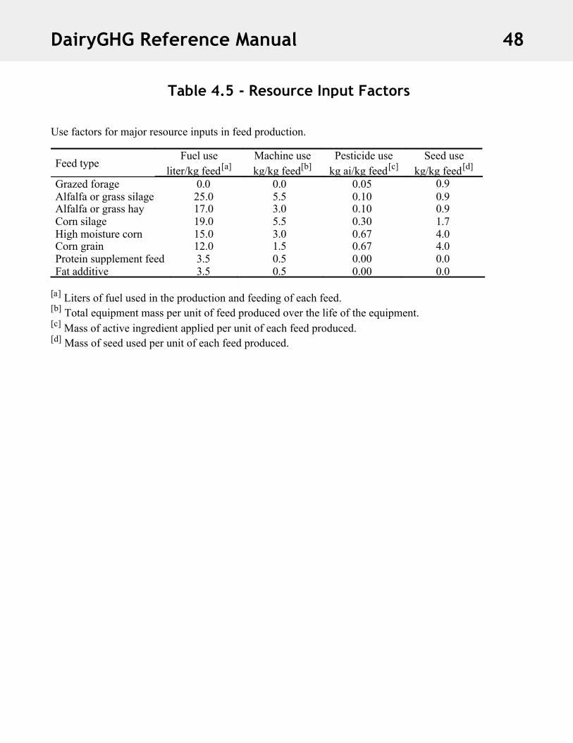
Table 4.5 - Resource Input Factors

Use factors for major resource inputs in feed production.

[a] Liters of fuel used in the production and feeding of each feed.[b] Total equipment mass per unit of feed produced over the life of the equipment.[c] Mass of active ingredient applied per unit of each feed produced.[d] Mass of seed used per unit of each feed produced.

Feed typeFuel use

liter/kg feed[a]Machine usekg/kg feed[b]

Pesticide usekg ai/kg feed[c]

Seed usekg/kg feed[d]

Grazed forage 0.0 0.0 0.05 0.9Alfalfa or grass silage 25.0 5.5 0.10 0.9Alfalfa or grass hay 17.0 3.0 0.10 0.9Corn silage 19.0 5.5 0.30 1.7High moisture corn 15.0 3.0 0.67 4.0Corn grain 12.0 1.5 0.67 4.0Protein supplement feed 3.5 0.5 0.00 0.0Fat additive 3.5 0.5 0.00 0.0


Association of Polymer Manufacturers in Europe (AMPE). 2008. Eco-profiles of the European Plastics Industry. Available at: http://lca.plasticseurope.org/main2.htm, Accessed March 2008. Bath M., B. English, A. Turhollow, and H. Nyangito. 1994. Energy in synthetic fertilizers and pesticides: revisited. Oak Ridge National Laboratory. ORNL/sub/90-99732/2. Available at: http://www.osti.gov/energycitations/servlets/purl/10120269-p6yhLc/webviewable/10120269.PDF. Benchaar, C., J. Rivest, C. Pomar, and J. Chiquette. 1998. Prediction of methane production from dairy cows using existing mechanistic models and regression equations. J. Anim. Sci. 76:617-627. Borjesson, P. 1996. Energy analysis of biomass production and transportation. Biomass and Bioenergy 11(4):305-318. Bowers, W. 1992. Agricultural field equipment. p. 117-129. In Fluck, R. (ed). Energy in Farm Production. Elsevier Amsterdam. Bruce, J.P., M. Frome, E. Haites, H. Janzen, R. Lal, and K. Paustian. 1999. Carbon sequestration in soils. J. Soil Water Conserv. 54(1): 382 – 389. Cederberg, C. and M. Stadig. 2003. System expansion and allocation in life cycle assessment of milk and beef production. Int. J. LCA 8(6):350-356. Chadwick, D.R. and B.F. Pain. 1997. Methane fluxes following slurry applications to grassland soils: laboratory experiments. Agr. Ecosyst. Environ. 63:51 – 60. Chastain, J.P., M.B. Vanotti, and M.M. Wingfield. 2001. Effectiveness of liquid-solid separation for treatment of flushed dairy manure: a case study. Appl. Eng. Agric. 17(3):343-354. Chen, Y.R., and A.G. Hashimoto. 1980. Substrate utilization kinetic model for biological treatment processes. Biotechnol. Bioeng. 22: 2081 – 2095. Chianese, D.S., C.A. Rotz, and T.L. Richard. 2009. Whole-Farm Greenhouse Gas Emissions: A Review with Application to a Pennsylvania Dairy Farm. Applied Eng Agric. (in press). Dalgaard T., N. Halberg and J. Porter. 2001. A model for fossil energy use in Danish agriculture used to compare organic and conventional farming. Agric., Ecosys. Environ. 87:51-65. Davidson, E.A., M. Keller, H.E. Erickson, L.V. Verchot, and E. Veldkamp. 2000. Testing a conceptual model of soil emissions of nitrous and nitric oxide. Bioscience 50(8):667 – 680. Doering O. 1980. Accounting for energy in farm machinery and buildings. p. 9-21. In Pimentel, D. (ed) Handbook of Energy Utilization in Agriculture. CRC press Inc. Boca Raton, FL. Environmental Protection Administration (EPA). 1999. U.S. methane emissions 1990 – 2020: Inventories, projections, and opportunities for reductions. EPA 430-R-99-013. U.S. Environmental Protection Agency, Washington, D.C. Available at: http://www.epa.gov/ghginfo. Accessed 23 November 2007.

REFERENCES


Environmental Protection Administration (EPA). 2008a. Inventory of U. S. greenhouse gas emissions and sinks: 1990-2006. USEPA #430-R-08-005. Additional Information. U.S. Environmental Protection Agency. 1200 Pennsylvania Avenue, N. W. Washington, DC. Available at http://www.epa.gov/climatechange/emissions/downloads/08_Annex_6.pdf. Accessed 9 July 2008. Environmental Protection Administration (EPA). 2008b. Nitrous oxide: Sources and emissions. W a s h i n g t o n , DC: U.S. Environmental Protection Agency. Available at:http://www.epa.gov/nitrousoxide/sources.html. Accessed 13 June 2008. Energy Information Administration (EIA). 2006. Emissions of greenhouse gases in the United States 2005. DOE/EIA-0573 (2004). U.S. Department of Energy, Washington, D.C. Available at:http://www.eia.doe.gov/oiaf/1605/ggrpt/. Accessed 12 November 2007. Fales, S.L., L.D. Muller, S.A. Ford, M. O’Sullivan, R.J. Hoover, L.A. Holden, L.E. Lanyon, and D.R. Buckmaster. 1995. Stocking rate affects production and profitability in a rotationally grazed pasture system. J. Prod. Agric. 8(1):88-96. Farrell A., R. Plevin, B. Turner, A. Jones, M. O’Hare, and D. Kammen. 2006. Ethanol can contribute to energy and environmental goals. Science 311:506-508. (January 27). Online Supporting Material. Available at: http://www.sciencemag.org/cgi/content/full/311/5760/506/DC1. Accessed 9 July 2008. Fluck, R. 1992. Energy analysis for agricultural systems. p. 45-52. In Fluck, R. (ed). Energy in Farm Production. Elsevier Amsterdam. Fox, D.G, L.O. Tedeschi, T.P. Tylutki, J.B. Russell, M.E. Van Amburgh, L.E. Chase, A.N. Pell, and T.R. Overton. 2004. The Cornell net carbohydrate and protein system model for evaluating herd nutrition and nutrient excretion. Anim. Feed Sci. Technol. 112:29-78. García-Ochoa, F., V.E. Santos, L. Naval, E. Guardiola, and B. López. 1999. Kinetic model for anaerobic digestion of livestock manure. Enzyme Microb. Tech. 25:55-60

Garrain D., P. Martinez, and R. Vidal. 2007. LCA of thermoplastics recycling. Proc. 3rd International Conference of Life Cycle Assessment. Zurich, August 27-29. Available at:http://www.lcm2007.org/paper/168.pdf. Accessed 9 July 2008. Graboski, M. 2002. Fossil energy use in the manufacture of corn ethanol. Colorado School of Mines. National Corn Growers Association. Available at:http://www.ncga.com/ethanol/pdfs/energy_balance_report_final_R1.PDF. Accessed 9 July 2008. Groenestein, C.M. and H.G. Van Faasen. 1996. Volatilization of ammonia, nitrous oxide, and nitric oxide in deep-litter systems for fattening pigs. J. Agric. Eng. Res. 65:269 – 274. Harrison, J. Animal Science Department, Washington State University. Puyallup Research and Extension Center, 7612 Pioneer Way, Puyallup, WA 98371. Hill, D.T. 1982. A comprehensive dynamic model for animal waste methanogensis. Trans. ASAE 28(3):850-855.


Hill, D.T. 1991. Steady-state mesophilic design equations for methane production from livestock wastes. Trans. ASAE 34(5):2157-2163. Intergovernmental Panel on Climate Change (IPCC). 2007. Climate change 2007: The physical science basis. Contribution of Working Group I to the Fourth Assessment Report of the Intergovernmental Panel on Climate Change. Chapter 2, Changes in atmospheric constituents and in radiative forcing. Available at: http://www.ipcc.ch/pdf/assessment-report/ar4/wg1/ar4-wg1-chapter2.pdf. Accessed 28 November 2008. Intergovernmental Panel on Climate Change (IPCC). 2001. Climate change 2001: The scientific basis. Contribution of Working Group I to the third assessment report of the Intergovernmental Panel on Climate Change. J.T. Houghton, Y. Ding, D.J. Griggs, M. Noguer, P.J. van der Linden, X. Dai, K. Maskell, and C.A. Johnson, eds. Cambridge University Press, Cambridge, United Kingdom and New York, NY, USA. Intergovernmental Panel on Climate Change (IPCC). 2006. Guidelines for national greenhouse inventories. Volume 3, p.3.75. Available at:http://www.ipcc-nggip.iges.or.jp/public/2006gl/pdf/3_Volume3/V3_3_Ch3_Chemical_Industry.pdf Accessed 9 July 2008. Jarvis, S.C., R.D. Lovell, and R. Panayides. 1995. Patterns of methane emission from excreta of grazing animals. Soil Biol. Biochem. 27(12):1581 – 1588. Jungbluth, T., E. Hartung, and G. Brose. 2001. Greenhouse gas emissions from animal houses and manure stores. Nutr. Cycle Agroecosyst. 60:133-145. Kirchgessner, M., W. Windisch, H.L. Müller, and M. Kreuzer. 1991. Release of methane and of carbon dioxide by dairy cattle. Agribiol. Res., 44(2-3):91-102. Kitzes, J., M. Wackernagel, J. Loh, A. Peller, S. Goldfinger, D. Cheng, and K. Tea. 2008. Shrink and share: humanity’s present and future ecological footprint. Phil. Trans. Biol. Sci. 363:467-475. Külling, D.R., H. Menzi, F. Sutter, P. Lischer, and M. Kreuzer. 2003. Ammonia, nitrous oxide and methane emissions from differently stored dairy manure derived from grass- and hay-based rations. Nutr. Cycl. Agroecosyst. 65: 13 – 22. Lal, R. 2004. Soil carbon sequestration impacts on global climate change and food security. Science5677:1623 – 1627. Lee, J., H. Cho, J. Sung, S. Lee and M. Shin. 2000. Life cycle assessment of tractors (Korean Example). LCA Case Studies. International J. Life Cycle Assessment 5(4)205-208. Ludington, D. and E.L. Johnson. 2003. Dairy farm energy audit summary. FlexTech Services. New York State Energy Research and Development Authority. Albany, NY. http://www.nyserda.org/publications/ dairyfarmenergysummary.pdf Accessed May 18, 2009. Mertens, D.R. 1997. Creating a system for meeting the fiber requirements of dairy cows. J. Dairy Science. 80:1463-1481.


Mertens, D.R. 1992. Nonstructural and structural carbohydrates. In Large Dairy Herd Management eds. H.H. Van Horn and C.J. Wilcox. Pp 219-234. Am. Dairy Sci. Assoc., Champaign, IL. Mertens, D.R. 1987. Predicting intake and digestibility using mathematical models of rumen function. J. Animal Science. 64(5):1548-1558. Meyer, D. 1997. Alternatives to manure management problems. p. 58-65. In Proc. Western Dairy Management Conf., Las Vegas, Nevada. Mills, J.A.N., E. Kebreab, C.M. Yates, L. A. Crompton, S. B. Cammell, M.S. Dhanoa, R.E. Agnew, and J. France. 2003. Alternative approaches to predicting methane emissions from dairy cows. J. Anim. Sci.81(12):3141-3150. Monteny, G.J., C.M. Groenestein, and M.A. Hilhorst. 2001. Interactions and coupling between emissions of methane and nitrous oxide from animal husbandry. Nutr. Cycl. Agroecosyst. 60:123-132. Nagy, C. 1999. Energy coefficients for agriculture inputs in western Canada. Canadian Agricultural Energy End-Use Data Analysis Centre (CAEEDAC). Available at:http://www.csale.usask.ca/PDFDocuments/energyCoefficientsAg.pdf. Accessed 9 July 2008.

National Research Council. 1989. Nutrient requirements of dairy cattle. 6th rev. ed. Natl. Acad. Sci., Washington, DC. National Research Council. 2000. Nutrient Requirements of Beef Cattle – update 2000. National Academy Press. National Research Council. 2001. Nutrient requirements of dairy cattle. 7th rev. ed.: Natl. Acad. Sci., Washington, D.C. National Research Council. 2003. Air emissions from animal feeding operations: current knowledge, future needs. Natl. Acad. Sci., Washington, DC. Olesen, J.E., K. Schelde, A. Weiske, M.R. Weisbjerg, W.A.H. Asman, and J. Djurhuus. 2006. Modelling greenhouse gas emissions from European conventional and organic dairy farms. Agric. Ecosyst. Environ.112:207 – 220. Ott, P., S. Hansen, and H. Vogtmann. 1983. Nitrates in relation to composting and use of farmyard manures. p. 145-154. In Lockeretz, W. (ed) Environmentally Sound Agriculture. Praeger Scientific, New York, NY. Parton, W.J., A.R. Mosier, D.S. Ojima, D.W. Valentine, D.S. Schimel, K. Weier, and A.E. Kulmala.1996. Generalized model for N2 and N2O production from nitrification and denitrification. Global Biogeochem. Cy. 10(3):401 – 412. Parton, W.J., E.A. Holland, S.J. Del Grosso, M.D. Hartman, R.E. Martin, A.R. Mosier, D.S. Ojima, and D.S. Schimel. 2001. Generalized model for NOx and N2O emissions from soils. J. Geophys. Res. 106(D15):17403 – 17419.


Pennsylvania Agricultural Statistics Service (PASS). 2008. Pennsylvania Agricultural Statistics, prices received. http://www.nass.usda.gov/QuickStats/index2.jsp Accessed January 10, 2009. Patel, M. 1999. Closing carbon cycles; carbon use for materials in the context of resource efficiency and climate change. Thesis Utrech University. Faculty of Chemistry. Utrech, the Netherlands. Patzek, T. 2004. Thermodynamics of the corn-ethanol biofuel cycle. Critical reviews in Plant Sciences. 23(6):519-567. Paul, J.W. and E.G. Beauchamp. 1989. Relationship between volatile fatty acids, total ammonia, and pH in manure slurries. Biol. Waste. 29:313 – 318. Pimentel, D. 1980. Energy inputs for the production, formulation, packaging and transport of various pesticides. Pages 45-48. In Pimentel, D. (ed) Handbook of Energy Utilization in Agriculture. CRC press Inc. Boca Raton, Florida. Rotz, C.A., D.R. Buckmaster, D.R. Mertens, and J.R. Black. 1989. DAFOSYM: a dairy forage system model for evaluating alternatives in forage conservation. J. Dairy Science. 72:3050-3063. Rotz, C.A., M.S. Corson, D. S. Chianese, and C.U. Coiner. 2008. Integrated Farm System Model: Reference Manual. Pasture Systems and Watershed Management Research Unit, USDA Agricultural Research Service: University Park, PA. Available at: http://www.ars.usda.gov/Main/docs.html?docid=8519. Accessed 31 August 2008. Rotz, C. A., D.R. Mertens, D.R. Buckmaster, M.S. Allen, and J.H. Harrison. 1999. A dairy herd model for use in whole farm simulations. J. Dairy Sci. 82:2826-2840. Sahrawat, K.L. and D.R. Keeney. 1986. Nitrous oxide emissions from soils. Adv. Soil Sci. 4:103-148. Savoie, P. and J.C. Jofriet. 2003. Silage storage. p. 405-467 In Buxton, D.R., R.E. Muck, and J.H. Harrison (eds). Silage Science and Technology. Agronomy Monograph 42, Madison, WI: American Society of Agronomy. Schroll, H. 1994. Energy flow and ecological sustainability in Danish agriculture. Agric. Ecosys. Environ. 51 (1994):301-310. Sedorovich, D., C.A. Rotz, and T.L. Richard. 2007. Greenhouse gas emissions from dairy farms. ASABE Paper No. 074096. St. Joseph, MI: American Society of Agricultural and Biological Engineers. Schmer, M., K. Vogel, R. Mitchell, and R. Perrin. 2008. Net energy of cellulosic ethanol from switchgrass. Proc. National Academy Sciences 105(2):464-469. Sherlock, R.R., S.G. Sommer, R.Z. Khan, C.W. Wood, E.A. Guertal, J.R. Freney, C.O. Dawson, and K.C. Cameron. 2002. Emission of ammonia, methane and nitrous oxide from pig slurry applied to a pasture in New Zealand. J. Environ. Qual. 31:1491-1501. Sneath, R.W., F. Beline, M.A. Hilhorst, and P. Peu. 2006. Monitoring GHG from manure stores on organic and conventional dairy farms. Agr. Ecosyst. Environ. 112:122-128.


Sommer, S.G. 2001. Effect of composting on nutrient loss and nitrogen availability of cattle deep litter. Europ. J. Agronomy 14:123-133. Sommer, S.G., S.O. Petersen, and H.B. Møller. 2004. Algorithms for calculating methane and nitrous oxide emissions from manure management. Nutr. Cycl. Agroecosyst. 69:143-154. Sommer, S.G., R.R. Sherlock, and R.Z. Khan. 1996. Nitrous oxide and methane emissions from pig slurry amended soils. Soil Biol. Biochem. 28(10/11):1541-1544. Tyrrell, H.F., P.W. Moe, and W.P. Flatt. 1970. Influence of excess protein intake on energy metabolism of the dairy cow. In Energy Metabolism of Farm Animals, eds. A. Schurch and C. Wenk. Page 69 Proc. 5th Symp. Energy Metab., Eur. Assoc. Anim. Prod. Publ. No. 13. Juris Druck and Verlag Zurich, Vitznau, Switzerland.. Van Horn, H.H., G.L. Newton, R.A. Nordstedt, E.C. French, G. Kidder, D.A. Graetz, and C.F. Chambliss. 1991. Dairy manure management: strategies for recycling nutrients to recover fertilizer value and avoid environmental pollution. p. 1-31. Florida Coop. Ext. Serv. Univ. Florida. Available athttp://edis.ifas.ufl.edu/BODY_DS096. van Hulzen, J.B., R. Segers, P.M. van Bodegom, and P.A. Leffelaar. 1999. Temperature effects on soil methane production: an explanation for observed variability. Soil Biol. Biochem. 31:1919 -1929. Wang, M. 2007. GREET version 1.8a. Argonne National Laboratory, Available at:http://www.transportation.anl.gov/software/GREET/. Accessed January, 2008. Weiss, W.P., H.R. Conrad, and N.R. St. Pierre. 1992. A theoretically-based model for predicting total digestible nutrient values of forages and concentrates. Anim. Feed Sci. Tech. 39:95-110. West, T. and G. Marland. 2002. A synthesis of carbon sequestration, carbon emissions, and net carbon flux in agriculture: comparing tillage practices in the United States. Agric., Ecosys. Environ. 91:217-232. Wilkerson, V.A., D.P. Casper, and D.R. Mertens. 1995. The prediction of methane production of Holstein cows by several equations. J. Dairy Sci. 78:2402-2414. Wu M., M. Wang, and H. Huo. 2006. Fuel-Cycle Assessment of selected bioethanol production pathways in the United States ANL/ESD/06-7. Center for Transportation Research. Energy Systems Division, Argonne National Laboratory. Available at:http://www.transportation.anl.gov/pdfs/TA/377.pdf, Accessed 9 July, 2008. Yamulki, S., S.C. Jarvis, and P. Owen. 1999. Methane emission and uptake from soils as influenced by excreta deposition from grazing animals. J. Environ. Qual. 28: 676 – 682. Zeeman, G. 1994. Methane production/emission in storages for animal manure. Fert. Res. 37:207-211. Zeikus, J.G., and M.R. Winfrey. 1976. Temperature limitation of methanogenesis in aquatic sediments. Appl. Environ. Microbiol. 31:99 – 107.
