NASA CR-

D2-118544-1 / d

MATHEMATICAL MODEL-FOR THE SIMULATIONOF DYNAMIC DOCKING TEST SYSTEM (DDTS)

ACTIVE TABLE MOTION

(NASA-CR-140288) MATHEMATICAL MODEL FOR N74-33776'THE SIMULATION OF DYNAMIC DOCKING TESTSYSTEM (DDST) ACTIVE TABLE MOTION (BoeingAerospace Co., Houston, Tex.) 57 p HC Unclas$6.00 CSCL 14B G3/11 49642

labn

THE F'f W COMPANY

HOUSTON, TEXAS

August 30, 1974

https://ntrs.nasa.gov/search.jsp?R=19740025663 2018-11-05T09:43:05+00:00Z

DOCUMENT NO. D2-118544-1

MATHEMATICAL MODEL FOR THE SIMULATIONOF DYNAMIC DOCKING TEST SYSTEM (DDTS)

ACTIVE TABLE MOTION

Contract NAS 9-13136

August 30, 1974

Prepared by

R. M. GatesD. L.- Graves

Approved by

R. K. NunoTechnical Program Manager

BOEING AEROSPACE COMPANY

Houston, Texas

D2-118544-1

REVISIONS

REV. DESCRIPTION DATE APPROVED

Form HOU3-1116 (LSS) Appro-d 11/67 AJT

D2-118544-1

ABSTRACT

This document describes the mathematical model developed to describe the

three-dimensional motion of the Dynamic Docking Test System (DDTS) active

table. The active table is modeled as a rigid body supported by six

flexible hydraulic actuators which produce the commanded table motions.

Key Words

Docking Simulator

Dynamic Docking Test System (DDTS)

Equations of Motion

Hydraulic Actuator

Mathematical Model

Motion Simulator

iii

D2-118544-1

TABLE OF CONTENTS

SECTION PAGE

REVISIONS ii

ABSTRACT AND KEY WORDS iii

TABLE OF CONTENTS iv

LIST OF ILLUSTRATIONS v

REFERENCES vi

1.0 INTRODUCTION 1-1

2.0 COORDINATE SYSTEMS AND TRANSFORMATIONS 2-1

3.0 TABLE MOTION COMMANDS 3-1

4.0 SERVO ELECTRONICS 4-1

5.0 ACTUATOR MODEL 5-1

6.0 EQUATIONS OF MOTION 6-1

7.0 CALCULATION OF ACTUATOR VELOCITIES AND POSITIONS 7-1

APPENDIX - NOMENCLATURE A-1

iv

D2-118544-1

ILLUSTRATIONS

FIGURE PAGE

1-1 DDTS Simulator Facility 1-2

2-1 Active Table Coordinate Systems 2-2

2-2 Euler Angles 2-3

2-3 Actuator Transformation Angles 2-5

4-1 Servo Electronics Block Diagram 4-2

5-1 Hydraulic Actuator 5-2

5-2 Hydraulic Servo Valve Schematic 5-4

6-1 Mass Matrix 6-15

V

D2-118544-1

REFERENCES

1. D2-118544-2, "Dynamic Docking Test System (DDTS) Active Table Computer

Program NASA Advanced Docking System (NADS)," August 30, 1974.

2. Merritt, H. E., Hydraulic Control Systems, John Wiley & Sons Inc.,

1967.

vi

D2-118544-1

1.0 INTRODUCTION

The development of the three-dimensional mathematical model and computer

program which simulates the dynamic motion of the DDTS active table in

response to table motion commands is documented in two volumes. Volume 1

presents the derivation of the mathematical model and Volume 2 (Reference

1) describes the resulting computer program, "NASA Advanced Docking System

(NADS)."

The active table shown in Figure 1-1 is modeled as a rigid body, and each

of the six actuators is modeled as a flexible rod with pinned ends. The

model includes nonlinear hydraulic equations for the hydraulic actuators

and a mathematical representation of the electronic control system for each

actuator. Actuator position, velocity, and differential pressure across

the hydraulic piston are used as feedback signals in the control system.

The nomenclature used in the equations is shown in the Appendix.

1-1

APOLL /SOYUIZ DCKING E ow su

- +,

a+

SFLOOR 9EAM S ECTION

SUPEA TRUCTURE jCO

ACTJATO uL LLY LOAD CELLEXTENDED ADAP TE

eACKSTOP -ACTIVE TABLE

uPPER SWIVEL JMINT

- cruAo / /

Figure 1-1. DDTS Simulator Facility

D2-118544-1

2.0 COORDINATE SYSTEMS AND TRANSFORMATIONS

2.1 INERTIAL COORDINATES (xI, YI, ZI)

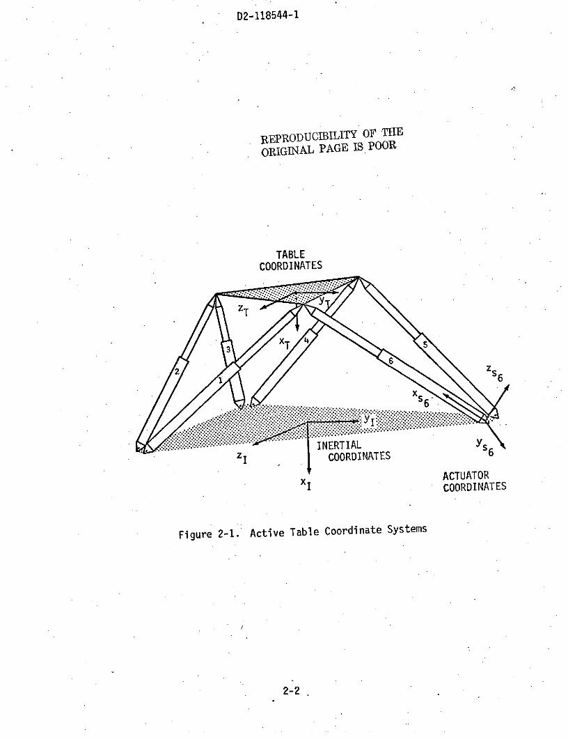
The inertial simulator coordinate system is an orthogonal, right-handed

coordinate system whose origin is on the simulator centerline in the plane

of the floor swivel joints. The yl and zI axes form a horizontal

plane, and the xI axis is positive down (see Figure 2-1).

2.2 TABLE COORDINATES (xT, YT' ZT)

The table coordinate system is an orthogonal, right-handed coordinate

system whose origin is at the center of gravity of the simulator

table.

The YT and ZT axes lie in the plane of the table, and the xT axis

is positive "down" (see Figure 2-1).

2.3 ACTUATOR COORDINATES (xsi, Ysi Zs

Each actuator has its own coordinate system. The xSi axis is colinear

with the actuator centerline. The ysi axis is perpendicular to the xsi

axis and the inertial gravity vector. The zsi axis is perpendicular to

both xs and y and is positive "up" as shown in Figure 2-1.

si Si

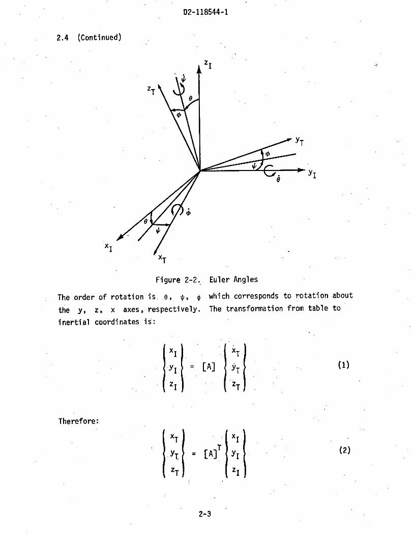
2.4 TRANSFORMATION FROM INERTIAL TO TABLE COORDINATES

Euler angles shown in Figure 2-2 are used to transform from inertial

coordinates to table coordinates.

2-1

D2-118544-1

REPRODUCIBILITY OF THE

ORIGINAL PAGE IS POOR

TABLECOORDINATES

ZT

2 s

S6..... -" 6

z INERTIAL S6zI COORDINATES

x ACTUATORxI COORDINATES

Figure 2-1. Active Table Coordinate Systems

2-2

D2-118544-1

2.4 (Continued)

zI

ZT

TYT

4YI

×Ix

IXT

Figure 2-2. Euler Angles

The order of rotation is e, p, * which corresponds to rotation about

the y, z, x axes, respectively. The transformation from table to

inertial coordinates is:

x xT

Y [A] Y (1)

z zT

Therefore:

xT x

YA [A]T j Y (2)

zT zI

2-3

D2-118544-1

2.4 (Continued)

. O cos _ sin xcosJ cosx

= sin .cos I y .(3)

1 -costanV sin~tanJ wz

Where:

[ Ce*C -C*Ce*S,+Seo*S S*CeO*S+C*-Se

[A] = SC*C* -S[CC] (4)

-SOeC C*-Se*S+S *Ce -S *Se*S+C*Ce

C = cosine

S = sine

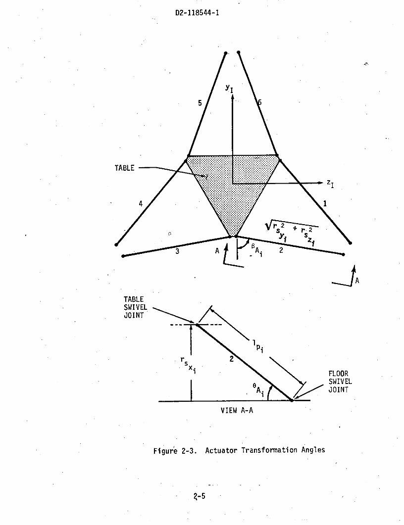
2.5 TRANSFORMATION FROM ACTUATOR TO INERTIAL COORDINATES

The transformation from actuator coordinates to inertial coordinates uses

the following angles:

eA - the angle between the horizontal plane through the floorjoint and the actuator xs axis (Figure 2-3)

8A - the angle between the inertial zI axis and the'projection

of the actuator xs axis in the y - zI plane (Figure 2-3)

rx

sin eA = 1 (5)i. Pi

r 2 +r 2 /yi Szi

cos A -1 (6)

Ai Ip

2-4

D2-118544-1

YI

5

TABLE

_2,TABLESWIVELJOINT

. FLOORSWIVELJOINT

VIEW A-A

Figure 2-3. Actuator Transformation Angles

. . . .

D2-118544-1

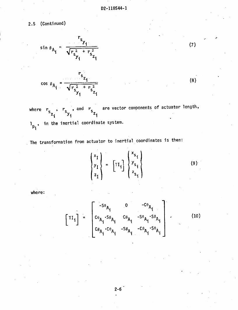
2.5 (Continued)

.Yi (7)sin $Ai rs2 + r 2

r$

S .1' (8)cos Ai r +r 2

y i zi

where r , r , and rs are vector components of actuator length,Zi Yi zi

Ipi, in the inertial coordinate system.

The transformation from actuator to inertial coordinates is then:

YI Si

where:

-SeAi 0 -CeAiA 1

TI CeAiSAi CAi -Se A*SA iA (10)

CBACe -SBA. -CBA.S

2-6

D2-118544-1

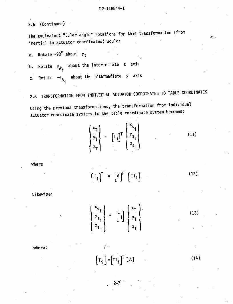
2.5 (Continued)

The equivalent "Euler angle" rotations for this transformation (from

inertial to actuator coordinates) would:

a. Rotate -900 about YI

b. Rotate BA about the intermediate z axisi

c. Rotate -eA about the intermediate y axis

2.6 TRANSFORMATION FROM INDIVIDUAL ACTUATOR COORDINATES TO TABLE COORDINATES

Using the previous transformations, the transformation from individual

actuator coordinate systems to the table coordinate system becomes:

YT = TiT ys (

zT zsi

where

[Ti T = [A]T [TIi] (12)

Likewise:

Yi T YT (13)zsi zT

where: /

[Ti =[T2i]T [A] (14)

2-7

D2-118544-1

3.0 TABLE MOTION COMMANDS

Table commands are specified in the inertial coordinate system. Actuator

commands for two types of commands will be discussed: sinusoidal position

commands and constant velocity commands,

3.1 SINUSOIDAL POSITION COMMANDS

Let AXI and Ae be the amplitude of commanded sinusoidal table

AyI

motion in the inertial coordinate system. The total inertial commands are

then obtained by adding the commanded sinusoidal motion to the initial

inertial position of the table.

x c x + AXI sin wct

YI = YI + Ay, sin Wct

C 0ZI Zsin ct

S = + Ae sin wctC 0 c

*c = o + A* sin wct (15)

c = o + A4 sin wct

Ic = Ax cos c t

I= AZ c cos ct

= Ae Cc cos wCt

= AOw COS w t

SA4w c cos ct

3-1

D2-118544-1

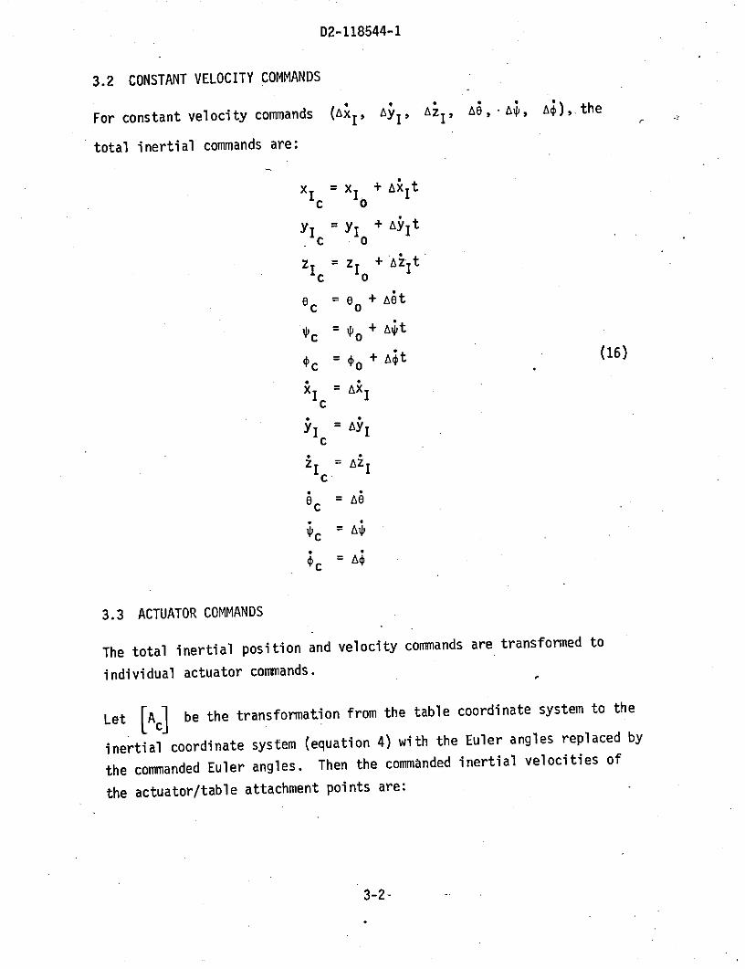
3.2 CONSTANT VELOCITY COMMANDS

For constant velocity commands (AI' AI' Az1 , A6, -A;, ' ), the

total inertial commands are;

x IC = x +&It

z = + Ait

I c I

;C

C = Ao

Zc =ai

3.3 ACTUATOR COMMANDS

The total inertial position and velocity commands are transformed to

individual actuator commands.

Let [Ac] be the transformation from the table coordinate system to the

inertial coordinate system (equation 4) with the Euler angles replaced by

the commanded Euler angles. Then the commanded inertial velocities of

the actuator/table attachment points are:

3-2-

D2-118544-1

3.3 (Continued)

As x - zC W rxas C + z 0 . - ryai (17)r .0l

. r

0 i -W W z a1rszi zc -c" zXc

where

xc 1 0 Sc c

Wyc =10 S CP *C c (18)

z 0 C, -C*,Sc ec

The commanded inertial components of actuator length are:

r x xasx c xaSx ra (19)

rs = Yc + Ac rya i i

rs z rza i zfi

zi c

Commanded actuator lengths are then:

S+ r + rs (20)

3-3

D2-118544-1

3.3 (Continued)

and commanded actuator velocities are:

ci - I rsxi rsxi + s rs + rs . rszi (21)

3-4

D2-118544-1

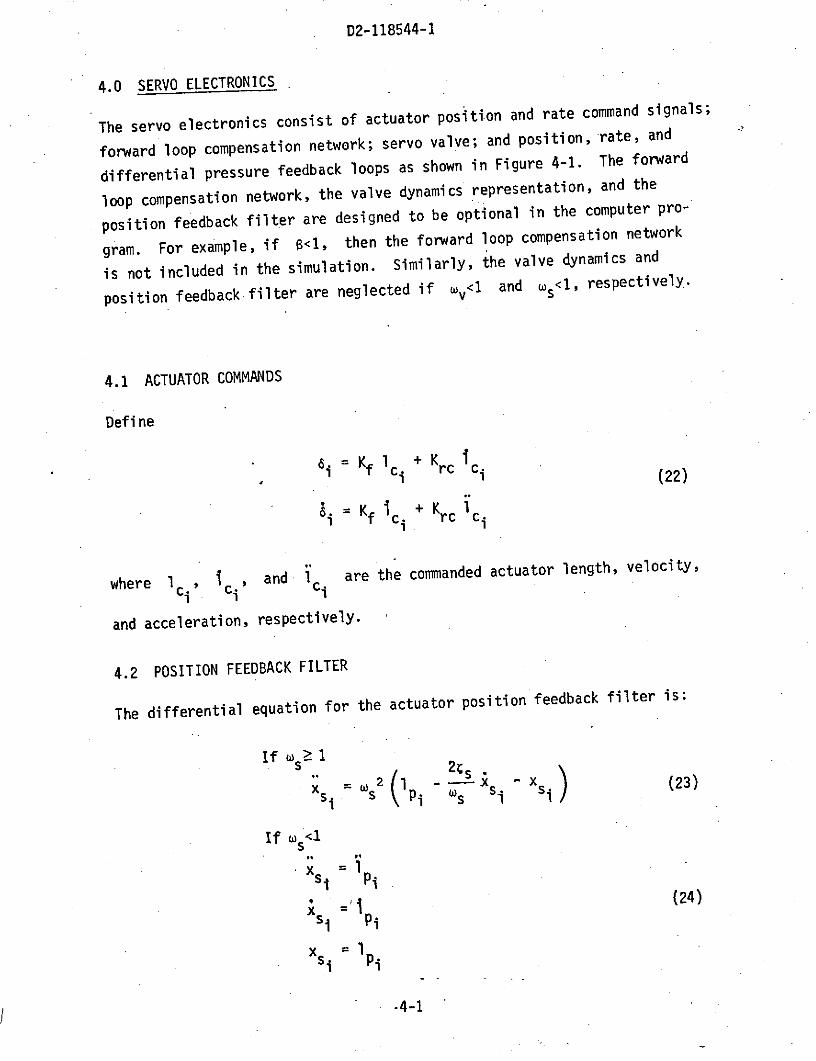
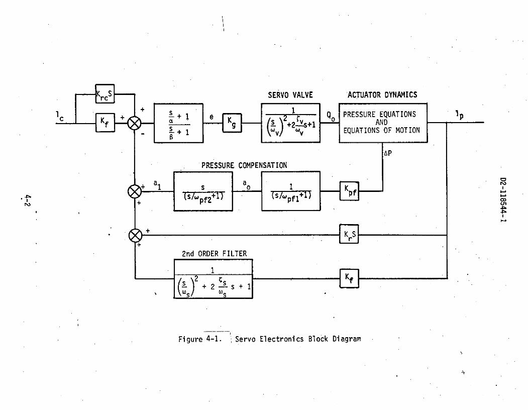
4.0 SERVO ELECTRONICS

The servo electronics consist of actuator position and rate command signals;

forward loop compensation network; servo valve; and position, rate, and

differential pressure feedback loops as shown in Figure 4-1. The forward

loop compensation network, the valve dynamics representation, and the

position feedback filter are designed to be optional in the computer pro-

gram. For example, if B<1, then the forward loop compensation network

is not included in the simulation. Similarly, the valve dynamics and

position feedback filter are neglected if v<1 and w <1, respectively.

4.1 ACTUATOR COMMANDS

Define

6 = Kf ci + Krc ci (22)

i = Kf i ci + Krc lci

where 1 ci ci, and 1c are the commanded actuator length, velocity,

and acceleration, respectively.

4.2 POSITION FEEDBACK FILTER

The differential equation for the actuator position feedback filter

is:

If >- 1s 2s

X s2(lpi -s - xs (23)

If (sil

*x =1xs Pi, -p (24)

s pi

xsi = pi

-4-1

-- SERVO VALVE ACTUATOR DYNAMICS

+ 1 e 2 1 Q PRESSURE EQUATIONS 1g a s +2 4+1 AND

+ 1 \"v/ v EQUATIONS OF MOTION

AP

PRESSURE COMPENSATION

a a K

(S/Wpf 2 +l) (S/wpf1+)

2nd ORDER FILTER

2 +2 s + l Kf

Figure 4-1. ,Servo Electronics Block Diagram

D2-11854 4 -1

4.3 DIFFERENTIAL PRESSURE FEEDBACK COMPENSATION

Pressure feedback compensation consists of two parts--a first-order lag

filter and a high-pass filter. The first-order lag attenuates

the higher

frequency pressure fluctuations, while the high-pass filter eliminates

the static differential pressure caused by unequal piston areas. The

differential equations for these filters are:

ai = pfFl IKpf I 1 - aoi(2(25)

a pf2 (oi - ali)

where Kpf is the pressure feedback gain.

4.4 FORWARD LOOP COMPENSATION NETWORK

The forward loop compensation network consists of a lead-lag

filter with

corner frequencies and B.

For o 1:

i i B ( i - 1 i -i Kf i (26)

a, Kr si - Kf x - ei]

where a, a1 , xs Xsl and x are signals from the feedback loops.

where i 1., al.,xs s s

For 8<1:

= 0

S- al Kr s - Kf xs (27)

where K and Kr are the displacement and rate feedback gains, respectively.

4-3

D2-118544-1

4.5 SERVO VALVE DYNAMICS

The dynamics of the servo valve are represented by a single-degree-of-

freedom system with a natural frequency wv and damping ratio v.

If Uv 1:

61o =v 2 ( K ei 2V Qoi) (28)

where K is the forward loop amplifier gain and Qo is the no-load

flow through the valve.

If Wv<l:

i =0 =0

S 1 (29)

Q =Kg ei

4-4-

D2-118544-1

5.0 ACTUATOR MODEL

Each actuator is modeled as a flexible rod with pinned ends. Hydraulic

forces are calculated using nonlinear hydraulic flow equations and unequal

push and pull piston areas. Actuator control system electronics are

modeled and include differential pressure, velocity, and position feedback.

The actuator geometry and nomenclature are shown in Figure 5-1.

5.1 ACTUATOR MASS AND INERTIA CHARACTERISTICS

The mass moment of inertia of the piston rod is:

m 12

m Ir2 (30)p 12

where mp is the driven mass (piston and piston rod). The mass moment

of inertia of the entire actuator assembly about the floor pivot is:

2.

I A1 I Ac + p + m 1 - (31)

where:

I Mass moment of inertia of the cylinder structure about the

Ac floor pivot (excludes driven mass, mp).

The effective rigid lateral mass of each actuator assembly for use in the

equations of motion is then:

mLi =IAi 1 2 (32)

5.2 ACTUATOR FLEXIBILITY

The dynamic bending characteristics of each actuator are calculated assuming

that the cylinder is rigid compared to the piston rod and that the effective

dynamic mass is lumped at the rod end seal of the cylinder. The bending

characteristics are also assumed to be identical for each of the two bending

planes of the actuator.

5-1

D2-118544-1

TABLE SWIVELJOINT

/ PISTON

Pi r

CYLINDER

FLOOR SWIVELJOINT

Figure 5-1. Hydraulic Actuator

5-2

D2-118544-1

5.2 (Continued)

The effective dynamic mass lumped at the cylinder end is approximated as:

mqi [IAc/ c2+mp/2] (33)

Assuming pinned joints between the cylinder and piston rod, the piston

rod stiffness is:

.3 (El)r 1rkr = 1 r (34)

r r1i r2i

where 1rli and 1r2 are defined as follows:

r r2 c

rl = i - c

r2 i r rl1 1

The effective lateral stiffness of the actuator with a rigid cylinder is:

3 (EI)r (lrlc - rliI lp ) (r + p i ) - (1c (35)

k = 1 r2 1 (35)e i rl i r2 i c r

The actuator bending frequency is then:

2 = k /m (36)

5.3 HYDRAULIC FLOW EQUATIONS

The nonlinear hydraulic flow equations are based on the derivations presented

in Reference 2 for. a double-acting hydraulic piston. A schematic of the

hydraulic servo valve and actuator is shown in Figure 5-2.

5-3

D2-118544-1

ACTUATOR

P1,V1,A1

Q, Q2

SPOOL

HYDRAULIC P HYDRAULIC PSUPPLY s RETURN oLINE LINE

Figure 5-2. Hydraulic Servo Valve Schematic

5-4

D2-118544-1

5.3 (Continued)

The flow continuity equations are:

V

(37)

Q2 = Cp (Pl " P2) Cep P2 "2 e 2

where:

Q1 = Qo - 2 Kc pl (38)

Q2 = Qo + 2 Kc P2

and

Qo = The no-load flow of the valve

Kc = Valve pressure flow coefficient

C = Leakage coefficient across the piston

C = Leakage coefficient past the piston rod seal

The volume-stroke relationships are:

V1 = Vo + A1(l - 1)

V2 =V - A2 (l - l )

91 =Al lp

2 = -A2 1p

where Vol and Vo2 are the hydraulic volumes at zero stroke.

5-5 -

D2-118544-1

5.3 (Continued)

Therefore, neglecting piston rod seal leakage, the hydraulic flow

equations

for each actuator are:

1 o - 2K p1 - Cp (P1 P2) - A1 i]

(40)

2 1 - 2K p2 + C (P1 P2)+ A2 pI]

5.4 ACTUATOR FORCES

Actuator forces F are calculated from the differential pressure

across the piston. In addition to the viscous damping forces associated

with the actuators, coulomb friction is also included.

Fp- A 1 A2P2 - Bp - CFFf (41)

A velocity "bandwidth" for coulomb friction is used to prevent a discontinuity

at zero velocity.Force

Ff

- Vbw

The coulomb friction force is:

FCF = -CF Ff (42)

5-6

D2-118544-1

5.3 (Continued)

where CF is a coefficient which is a function of actuator velocity:

Ft

Iflipl _ Vbw , then CF = P

lip (43)

If lip < Vbw , then CF Vbw

5-7-

D2-118544-1

6.0 EQUATIONS OF MOTION

Table and actuator equations of motion are written in the body fixed

table coordinates in the following form:

i = [M] - 1 (CI (44)

Where: lXi is a column of accelerations for each degree of freedom (six

degrees of freedom for the table and two elastic degrees of

freedom for each actuator)

[M] is the 18 x 18 coupled mass matrix

IC) is a column of generalized forces for each degree of freedom

The mass coupling effects of the actuators due to table motions are derived

by Lagrange's method.- The three-dimensional rigid motions of the actuators

are completely constrained (i.e., they are dependent upon the motions of

the table). These constraints are expressed by the velocity substitutions

in the energy expressions.

The final equations are much simplified when compared with the equations

which would result from a rigorous derivation. Due to the nonorthogonality

between actuator and table motions, a large number of nonlinear velocity

coupling terms results. All of these terms were assumed negligible since,

for expected table velocities, they are quite small and their omission

prevents the equations from becoming unwieldy.

6.1 MASS MATRIX

The kinetic energy of the rigid table and actuators is:

T + 6T=;-m T T(IT +T) + mp i1 Pi

1 (45)

+ f ~ (a2 + a 2) dmii= 6-1

6-1

D2-118544-1

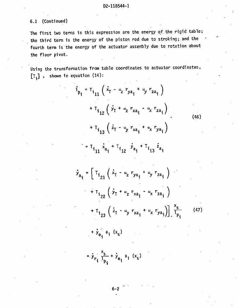
6.1 (Continued)

The first two terms in this expression are the energy of.the rigid table;

the third term is the energy of the piston rod due to stroking; and the

fourth term is the energy of the actuator assembly due to rotation about

the floor pivot.

Using the transformation from table coordinates to actuator coordinates,

[Ti] , shown in equation (14):

Ipi T 11( yai y rza

i12 (T wz xai "x zai12 ri(46)

+Ti3 (T - w rxai + Wxryai

= Ti Xa + Ti Ya + T.i Za11 1 i 12 ai 113 ai

ai Ti21 (XT- z ryai + y rza )+ T i22 + rxa rza

T T z x ~x za.

+ T 23 (zT - rxai +x rya ) i (47)

+ e i (xs)

x

=ri + Ye i *i (xs)

6-2

D2-118544-1

6.1 (Continued)

ai T31 T z ya y rzai

+Ti (T+z rxa "wx rza)32 ZT i i

+ T -w r + s (48)33 'T y xai + x ryai )] 1

ei i .(Xs)

ri Ip e i s)

where:

*i (Xs) is the actuator bending mode shape as a function of

xs , and Ye and ze are bending velocities of the

actuators.

The elastic bending modes of each actuator are assumed to be a simple

mode shape normalized to unity at the upper end of the cylinder (xs = 1 ).

There are two identical modes for each actuator. The generalized mass

for each mode is assumed to be lumped at the upper end of the cylinder;

thus, the mass distribution terms can be integrated.

e.g. 1foPi 2 IAixs dm = A = mass moment of total actuator assembly

about the floor pivot.

6-3

D2-118544-1

6.1 (Continued)

and:

f i xs (xs) dmi= Ic m i

where m is the generalized mass of ith actuator for each

qi

bending mode.

Lagrange's equation requires the determination of d -T where Qj is

ttj

the jth generalized coordinate in the equation of motion. In this simu-

lation:

41 = xT 7 el

Q2 =t Q8 = e1Q3 =T (49)

44 Tx

5 -WT QT17 e 6

Q6 "T z Q18 = ie 6 .

Then:

A mT rT rT aQ T

(50)

+ mP Pi + 6 P i " zai dmi=Ij i=1 j

6-4- -

D2-118544-1

6.1 (Continued)

For j < 6:

1BYa C (51)

j i I

where C are coefficients from equation (47). e.g.yij

yil= Ti21CYi I 21

Ci4 -Ti22 zai + 23 ya

etc.

For j = 7, 9, 11, 13, 15, 17:

ai _

aya . (52)

and, for j = 8, 10, 12, 14, 16, 18

a.aai-= 0 (53)

Likewise:

aiai xS s C for j 5 6 (54)

aQij pi ij

= 0 for j = 7, 9, 11, 13, 15, 17 (55)

= 1 for j = 8, 10, 12, 14, 16, 18 (56)

6-5

D2-118544-1

6.1 (Continued)

Therefore, for j 5 6, the last term in equation (50) becomes:

Sr i C + CYij ei ¢i (xs)Qj i=1 pi e

(57)2

Si zij Ipi C (xs) dmi='I .i + i z) i 1 Ze i

A ri y ri Cz)+ i ( C ei + Cz ei (58)

i=1 Pi j Ii

where, from equations (47) and (48):

=r Ti + Ti + T. (59)

ri 21 ai 22 ai '23 i

=T. +T fa +T i (60)ri i31 ai i32 ai 33 i (60)

and, from equation (46):

Xai = xT wz rya i + y rza i (61)

Yai = T + rxai - x rza (62)

Zai T - y rxai + x ryai (63)

6-6-

D2-118544-1

6.1 (Continued)

Also, for j = 7, 9, 11, 13, 15, 17, the last term in equation (50)

becomes:

S= , - i (xs) +e i i2 (X)) dmi (64)aQ 1 Pi

=M 1 i + (65)qi (ri I + ei

Likewise, for j = 8, 10, 12, 14, 16, 18:

1caT ic + ) (66)JQ 1i IPi

Differentiating equations (50), (58), (65), and (66) to obtain d (dT)j

for j < 6

d T =T T T a [T (IT T.. *

6 pi d alpmp: . + 1 PiJ

i=L j Pi Pi dt

l i - 2 IA 1i p'i) ( + r Czij

+ i "" + z - +ri C + - C+ (Yri C y Zri Czi j ij z

6-7

D2-118544-1

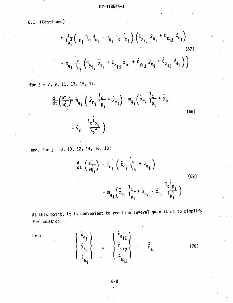
6.1 (Continued)

p+(lpi 1 q- mq 1 1 C yij + Czij ei

(67)

qi Ip j Ye i zij Zei + CYij ei

for j = 7, 9, 11, 13, 15, 17:

1 .. 1d T +dtqi ri lp i i i I Yei

(68)

i pi

and, for j = 8, 10, 12, 14, 16, 18:

(69)

1 z 1P

q+mi( ri . + -ei- ri 1Pi

At this point, it is convenient to redefine several quantities to simplify

the notation.

Let: I xa r ail

Yai ra E rai (70)

ai ra

6-8

D2-118544-1

6.1 (Continued)

also: C - 1 Tilj 2j(71)

C -Tzij 3j

Then equations (46), (59), and (60) become:

3

pi = Til aki (72)

3

r i r (73)

ri k=1 2k aki

3

i = Ti (74)ri k= i3k aki

Then, for j = 1, 2, 3:

P Ti (75)

ST.

aQj lj

3,

i T.k r (76)

Pi k=1 lk aik k aik

3

Yr i = Tik a i + Ti r (77)

k=1 2k ik 2k aik

3r + T r T. r (78)

ri k=l '3k aik i3k aik

6-9-

D2-118544-1

6.1 (Continued)

Therefore, for j = 1, 2, 3:

T -[j - row of mT ( + X T)]

6 3 .

P i lj = Tilk raik + lk raik

3 6

+T IT a] *A.j k= rak 1 i= Pi

3 3 "- 2 A i (T 2j Ti2k rai +T kTi3k rai

Ai Pi k=l ak k=1

+ 2j k= i2k aik 2k aik

3

+Ti Ti + T a3j k=1 3k a3k3k aik

3 3

+ T Ti raia + Ti E Ti rai2j k=1 2k k 3j k=1 3k ik

!+ l - mq 1 Ti2j ei + Ti3j ei

+ m - T2i i + Ti3 i i2j ei + Ti Zei (79)qi pi i2j Yi 3j jei

The general equations are extremely complex, particularly because of all

the centrifugal and coriolis acceleration terms. These terms can be shown

6-10

D2-118544-1

6.1 (Continued)

to be small (less than 0.01 g) for the expected table velocities.

Neglecting these terms, equation (79) becomes (for j = 1, 2, 3):

d(t T) = [ row of mT(T T

6 3

+ mp Ti l Ti raiki=1 j k=1 lik

6 I 3 3 (80)

6 1+ mq i T + Ti

=1 1

Likewise for j = 4, 5,-6:

= [row (j-3) of IT] T + T T T',t

6 l + A al I C

+ m i Yri Cyij +ri Czij (81)

6 l 1

= qi 1- CYij ei + Czij ei

where:

-T + T. r (82)BP i 12 rzai 13 ryai Cxx i

ip/.Pi (83)

.r l rz11 ai 13 rai Cxy i

6-11

D2-118544-1

6.1 (Continued)

-Ti ri 12 rxa C (84)

Define:

C =-T. r + T. r (85)

yi4 122 zai 23 yai yxi

= -T rza + T r C (86)

zi4 32 i 33

C = T21 rza - T r xa C (87)

i 21 i 23

C = -T r + T. r C (88)

yi6 21 ya i 22 xai yzi

Then, using equations (72), (73), and (74), equation (81) becomes:

d 2 - = [row (j-3) of [I] IT + T X ( *T)

6 31p a

+ mp Ti T ai=1 Q k=1 1k ik

(89)

6 I 3 3

(1 (CT 2k ik j k=l 3k raik

6 1

S mqi i j Yei + Czij zei

Simplifying equation (68), for j = 7, 9, 11, 13, 15, 17:

d cT

dt izmq i IpYri + Yei)

6-12-

D2-118544-1

6.1 (Continued)

1 3M + - Ti r (90)mqi ei mqi Pi k= 1 2k aik

and, simplifying equation (69), for j = 8, 10, 12, 14, 16, 18:

1 3d T +m Ti ra (9i)

dt / mi ei m qi Pi k= T1 3k a i k

Expanding some of the summations in equations (89), (90), and (91):

Ti r aik TT z rya i + y rza ik=1 1 1k 11ri T

+ Ti12 YT +wz rxai i x rza i (92)

+ T 13 T - y rxa i + x rya

Sr

aik = ( T z ryai +, rzai)

k= k aik 21 T z ya6-

6-13

D2-118544-1

6.1 (Continued)

+ Ti 2 T + z r xa " x rzai32 1

+ T 33 T y xai + x ryai (94)

Using the definitions in equations (82) through (88), these equations

reduce to:

3Ti ra Ti xT + Ti YT + Ti zT + Cxx

k=1 1k ik 11 12 13 xxi x

(95)+Cxy i y xzi z

3T r = T x + T YT +-Ti ZT + CY x

k=1 2k aik 21 T 22 23 Cyxi

(96)

+ C + C

3LT ra =T xT + Ti yT + T zT + Czx Wxk=1 3k ik 31 32 YT 3 3 iT zxi

(97)

zyi y Czzi z

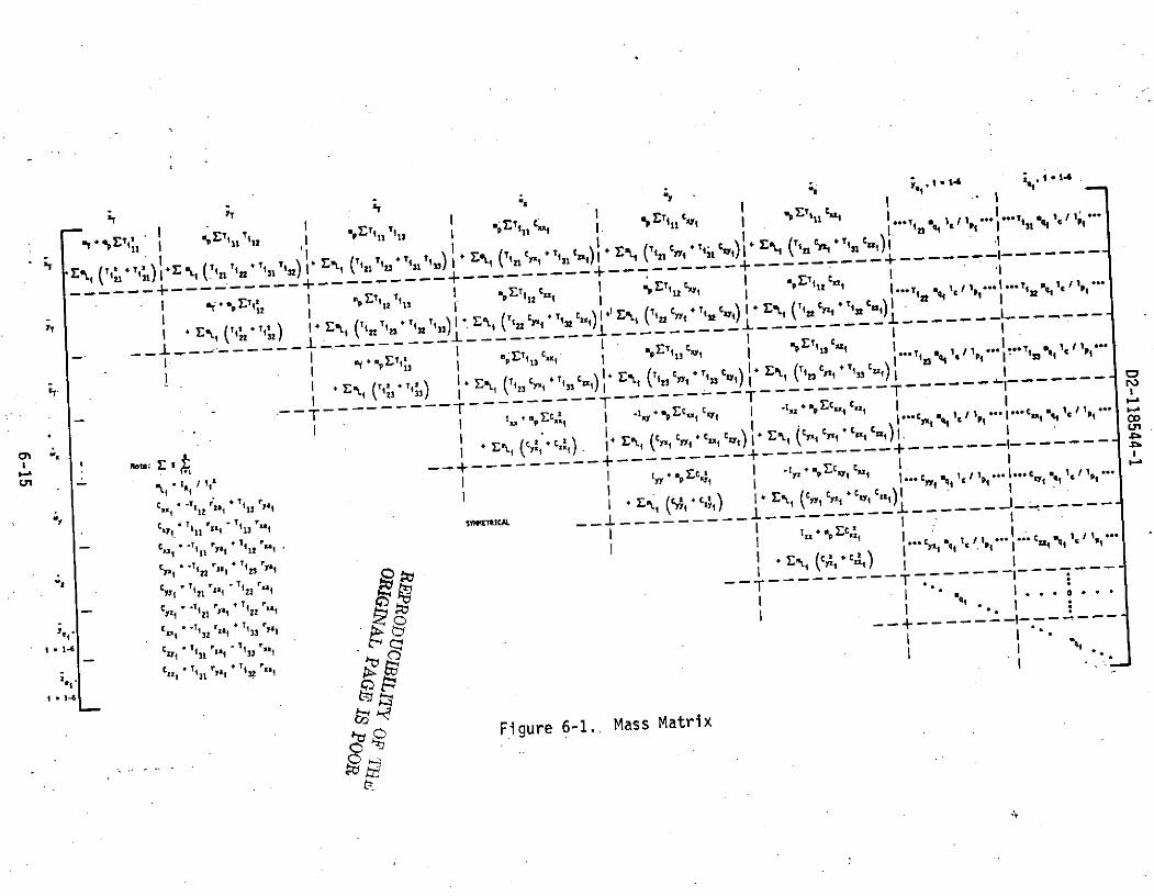
The mass matrix shown in upper triangular form shown in Figure 6-1 is

obtained by combining equations (95) through (97) and (82) through (88)

with equations (80), (89), (90), and (91).

6.2 GENERALIZED FORCES /

The generalized forces are obtained by considering the work required to

produce a unit displacement for each degree of freedom.

6-14

TilT p1 a I 0, Vill Cut ." T. , 91 c1 i 1 1 3 1 3 c 1'

4 'I

Ey" *2 Ell 1 3 I Till

1 * I*T t

T --

- - 3 - --- -- - ------- I - - --

ST 2 C I 2 n, (,,x , C . "" ". *'1Mote: . I s .,(x, C,) C_..C 1(1,:, 1 ,. o C, II e .1 ,,.

77 EO' T + 72 (T1 T2 + n Ti ) ., (7'2 C N I .- -,L, -' 122 -11 - -3

I +ill zai2 1 1p t 1 q 1 33

* 3 y T) ( t E11 1L (y * #il~ ( 1 c x1a (I Cz1 * 13 C Z1 C 4 9I

Cyn+tEN TT I Tit ER Cy 3 Ti32 rl - - - - -3 3) 12rza 1 Il ( *

_, - - .T.. .. T - ..... -T -- - - ..- - - - - - T I .y 4 i ,,Ec'' % c cin 4 "I Ec cx Ca l ... ...c % € I / l "

' * y* C 'i31 Czai " C33 rxam iZm I CA, + ; C 1 1+ 1) Ertl ( Y., Cyy + 1-1 EN (Up -CC - -1i -I - -C-1 1 - --- - - - -- -- + - -

C11 -T

EI( ) ( c ,, -C+ •. Y) , .Eft. (c C ), I 1 q "

C i Ti1 rt. + T 13 rxa "

- - - -- - -. .

C - 12 ,* ( C4, I * c ( Cra1- C l

.. Cq, C1 1)

Cy4 " 11 j , ",,1123 ,YI1

Uj C q 'ct. C •1 1c 11•C1

•1 'i , (A: .c,) , ---

-i CT j za 123

cyy .i zll ril. 2 3 Ty% N

.. . .

iT *

T

I11- C igu I

S61-6 Cl2 11

0 Figure 6-1., Mass Matrix

D2-118544-1

6.2 (Continued)

Wj = Qj (6qj) (98)

where:

Qj = Generalized force

sqj = Unit displacement

Let Fp be the net piston force along the local xs actuator axis. The

work done is then:

W = Fpi xsi (99)

But, since:

xsi xTyi= Ti T (100)

z TSi

then:

6W.i ,= F T. Ti Tj YT (101)

SFpi '11 12 T 13

zT

The generalized force for the table translational degrees of freedom are

obtained by letting xT = 1, yT = zT = 0 .and then YT = 1, xT = zT = 0,

etc.

6-16

D2-118544-1

6.2 (Continued)

6) F T.

FHx

6FHy F Ti 12 (102)

Hz 6ijlPi Ti

F•Pi T 13

The displacements at the table swivel joints due to rotations of the table

are:

AXi 0 -Aez AeYre xai

y =yi Aez 0 -Aex ryai (103)

Azi -Ae 0i T y x rza i

For Aex = 1, Aey = Az =0:

AXi 0

Ayi = -rza i (104)

Azi T rya i

For Aey =1, -A x Aez 0:

Ax.i rza

Ay = 0 (105)

Az xa

6-17

D2-118544-1

6.2 (Continued)

For Aoz = 1, A x = y = 0:

i = (106)

AZiT

Transforming these displacements to the servo actuator coordinate system:

Ax = -Ti rzai + T r yai for Aex = 1

si 112 1 13 a

AXs T rza - T r for Aey =1 (107)

isi 11 zai 13 xai

AX i = -T. r + T. r for Ae = 1si 11 yai '12 xai

Then:6

6W = Fpi AXsi (108)

i=1 1 1

or:

MHx 16 i Ti1 2 rza i i 13 r ya i )

z 6

1F " Ti r a i Ti rxai

F - T i rya + T'12 r /

These generalized forces are' combined with the mT (T X terms from

equation (80), the -T X (IT T) terms from equation (81), the actuator

6-18

D2-118544-1

6.2 (Continued)

damping and stiffness terms and the external forces and. moments to obtain

the ICI matrix of equation (44):

FH FEXT 0 z y xT x

F F

zT L-WY x 0 T F H z Ez

SM M=EMJ-1 -- + H + ME (110)

-------------------.-----------------

* = [MI z x x y y

S-2 eimqi zei We i ei

Ze . 16-i .19

6-19

D2-118544-1

7.0 CALCULATION OF ACTUATOR VELOCITIES AND POSITIONS

Actuator lengths and velocities are calculated from the equations of motion

.variables for use in the servo loop feedbacks and for the determination of -

actuator friction forces.

Actuator velocities are calculated by first determining the velocities

of

the actuator/table attachment points in table coordinates:

xT 0 -z y r xai

a. + YTI 0 -W(iira + z 0 -x ryai

ai iT -Wy x rzai3

These velocities are then transformed to actuator coordinates to obtain:

- 3

p = Ti k rai (112)

k=1 k

Actuator lengths are calculated by first obtaining the components of actuator

length in the inertial coordinate system.

rs x rxa 0

r s =YI + A rya i Yfi (113)

Yi I [ I (rs I rza z fzi i i

where yf and z are the inertial coordinates of the floor swivel joints

i i

of each actuator.

7-1 - -

D2-118544-1

7.0 (Continued).

Then the actuator lengths are calculated as follows:

1 r2+ r2 +r2Pi s s sz (114).

These actuator lengths. and velocities are used in the feedback loops inthe servo electronics shown in Figure 4-1.

7-2

APPENDIX

NOMENCLATURE .f

Symbol Description

[A] Transformation matrix from table to inertial coordinates

A1 , A2 ."Push" and "pull" stroke working areas of actuators

ao Output of the pressure feedback first-order lag filter

al Output of the pressure feedback high-pass filter

Bp Viscous damping coefficient of actuator

IC} Column of generalized forces for equations of motion

solution

C Leakage coefficient across piston seals

e Output of the forward loop compensation network

EIr Bending modulus of piston rod

FEXT External force

Ff Coulomb friction force of actuator

FH Total hydraulic and friction forces acting on pistons

Fp Net forces on actuator piston

I Inertia tensor of the active table

Mass moment of inertia of entire actuator assemblyA about floor pivot

Mass moment of inertia of cylinder (excluding the

AC mass of the piston) about floor swivel joint

I Mass moment of inertia of the piston rod

A-1- -

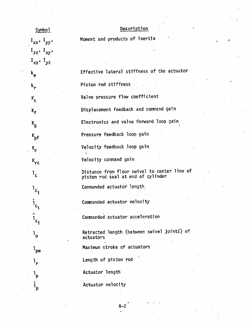
Symbol Description

xx yy, Moment and products of inertia

zz Ixy

Ixz Iyz

ke Effective lateral stiffness of the actuator

kr Piston rod stiffness

Kc Valve pressure flow coefficient

Kf Displacement feedback and command gain

Kg Electronics and valve forward loop gain

Kpf Pressure feedback loop gain

Kr Velocity feedback loop gain

Krc Velocity command gain

1 Distance from floor swivel to center line ofc piston rod seal at end of cylinder

1 Commanded actuator length

i Commanded actuator velocityci

1 Commanded actuator accelerationci

1 Retracted length (between swivel jointg) ofo actuators

1pm Maximum stroke of actuators

1r Length of piston rod

1 Actuator length

1i Actuator velocity

A-2

Symbol Description

1' Actuator acceleration

ml Effective rigid lateral mass of actuator assembly

Mass of piston rod and piston

Effective bending mass lumped at rod seal of cylinder

mq

mt Table mass

M, M-1 Mass matrix and mass matrix inverse

MEXT External moments

MH Moment acting about table c.g. from hydraulic and

friction forces

Ps Supply pressure

1' P2 "Eush" and "pull" actuator hydraulic pressure

jt h generalized coordinate

Qo No-load valve flow

Q1 ' Q2 Hydraulic flow into and out

of the actuator

Inertial vector components of actuator length

X axis table station of actuator swivel joints with

rxa respect to the table c.g.

ya rza Y, Z table coordinates of swivel joints with respect

rYa ' rza to the table c.g.

IT] Transformation matrix transforming vectors from table

coordinates to local actuator coordinates

[TI] Transformation from actuator to inertial coordinates

t Time

T Kinetic energy of the system

A-3.

Symbol Descr ption

Vbw Velocity bandwidth for coulomb friction

V Initial hydraulic volumes of push and pull strokes

o of fully retracted actuator

V1, V2 "Push" and "pull" hydraulic volumes

xI, yI, zl Inertial coordinates

xs' Ys, zs Actuator coordinates

XT' YT, ZT Table coordinates

yX Initial inertial coordinates of table c.g.

0

Ye, Ze Bending displacements of the actuators

yf' Zf Y and Z inertial coordinates of floor swivel joints

SBreak frequency of first order filter

Break frequency of first order filter

The angle between the inertial zI axis and the

projection of the actuator xs axis in the yi-zi

plane

e- Equivalent hydraulic system bulk modulus

Total actuator command signal

Sinusoidal amplitudes of translational commands for

Ax table c.g. and of table Euler angles

AZ, AO,

e, 9, * Euler angles

The angle between the yi-zi plane and the actuator

xs axis

A-4-

Symbol Description

e , %o' ,o Initial Euler angles of the table coordinate systemwith respect to the inertial system

Actuator bending mode shape

Ce Damping constant for actuator bending

,s Damping constant of second order filter on displacementfeedback

v Damping constant of valve dynamics

,1' W2 Break frequencies of first order filters

WC Displacement command signal frequency

We Actuator bending frequency

Wf Frequency of sinusoidal.external forces and moments

"pf1 , Wpf2 Break frequencies of pressure feedback filters

Ws Frequency of second order filter on displacementfeedback

mv Frequency of valve dynamics

Wx, Wy, z Table rotational rates

A-5