d1.3.2 continuous report on performance evaluation

Project funded by the European Commission within the Seventh Framework Programme (2007 – 2013)

Collaborative Project

GeoKnow -‐ Making the Web an Exploratory Place for Geospatial Knowledge

Deliverable 1.3.2 Continuous Report on Performance Evaluation

Dissemination Level Public

Due Date of Deliverable Month 12, 30/11/2013

Actual Submission Date 30/11/2013

Work Package WP1 -‐ Requirements, Design, Benchmarking, Component Integration

Task T1.3 -‐ Performance Benchmarking and Evaluation

Type Report

Approval Status Final

Version 1.0

Number of Pages 50

Filename D1.3.2_Continuous_Report_on_Performance_Evaluation.pdf

Abstract: The purpose of this deliverable is to summarize the performance evaluation of the GeoKnow components as developed within the first project year.

The information in this document reflects only the author’s views and the European Community is not liable for any use that may be made of the information contained therein. The information in this document is provided “as is” without guarantee or warranty of any kind, express or implied, including but not limited to the fitness of the information for a particular purpose. The user thereof uses the information at his/ her sole risk and liability.

Project Number: 318159 Start Date of Project: 01/12/2012 Duration: 36 months

D1.3.2 – v. 1.0

History Version Date Reason Revised by 0.0 19/11/2013 Initial Draft Mirko Spasić 0.1 21/11/2013 Initial Review Hugh Williams 0.2 25/11/2013 Summary, Acronyms, and Outline Mirko Spasić 0.3 26/11/2013 Figures and Tables Mirko Spasić 0.4 03/12/2013 Review Kostas Patroumpas 0.5 03/12/2013 Review Giorgos Giannopoulos 0.6 04/12/2013 Reviewer’s comments/suggestions added Mirko Spasić 0.7 06/01/2013 Final version Mirko Spasić Author List Organisation Name Contact Information OGL Hugh Williams [email protected] OGL Mirko Spasic [email protected] OGL Orri Erling [email protected] OGL Ivan Mikhailov [email protected] Time Schedule before Delivery Next Action Deadline Care of First version 19/11/2013 Mirko Spasić (OGL) Second version 06/01/2014 Mirko Spasić (OGL)

D1.3.2 – v. 1.0

Executive Summary

This deliverable will give an update of the setup and configuration of the GeoKnow Benchmarking laboratory and specification of the benchmarks to be used. The benchmark is expanded in order to be used against relational data. The improved procedure for migration of OSM data from PostGIS to Virtuoso is presented. Benchmark comparison results are presented running the FacetBench program against Virtuoso (SPARQL & SQL) and PostGIS both hosting OSM data. The analytical queries are developed, as well as the exporting results of them to the .dxf file.

D1.3.2 – v. 1.0

Abbreviations and Acronyms DXF Drawing Interchange Format ETL Extract, Transform, Load EWKT Extended Well-‐Known Text GIS Geographic Information System LGD Linked Geo Data LOD Linked Open Data OSM Open Street Map RDBMS Relational Database Management System SRID Spatial Reference System Identifier VOS Virtuoso Open Source WKT Well-‐Known Text

D1.3.2 – v. 1.0

Table of Contents 1. INTRODUCTION ......................................................................................................................................................... 7 1.1 OUTLINE.......................................................................................................................................................................................8

2. MIGRATION OF THE OSM DATA FROM POSTGRESQL TO VIRTUOSO....................................................... 9 2.1 GLOBAL IDEA...............................................................................................................................................................................9 2.2 SCHEMA CHOICES .....................................................................................................................................................................10 2.3 MIGRATION PROCEDURES ......................................................................................................................................................10 2.4 ETL PERFORMANCE ANALYSIS .............................................................................................................................................14

3. BENCHMARK RESULTS ..........................................................................................................................................16 3.1 DATASETS .................................................................................................................................................................................16 3.2 LGD BULK LOAD .....................................................................................................................................................................17 3.3 OSM BULK LOAD OVER SQL FEDERATION.........................................................................................................................19 3.4 VIRTUOSO SPARQL RESULTS ...............................................................................................................................................19 3.5 VIRTUOSO SQL RESULTS ........................................................................................................................................................20 3.6 POSTGIS SQL RESULTS ..........................................................................................................................................................23 3.7 RESULTS COMPARISON ...........................................................................................................................................................24

4. QUERY PLANS ...........................................................................................................................................................27 4.1 POSTGIS QUERY PLANS .........................................................................................................................................................27

5. GRID DIVISION .........................................................................................................................................................28 6. ANALYTICAL QUERIES ...........................................................................................................................................30 6.1 PRODUCING DXF .....................................................................................................................................................................31

7. CONCLUSION .............................................................................................................................................................34 8. APPENDIX ..................................................................................................................................................................35 8.1 POSTGIS QUERY PLANS...........................................................................................................................................................35 8.2 GRID DIVISION..........................................................................................................................................................................36 8.3 EXECUTION OF THE ANALYTICAL QUERIES .........................................................................................................................38 8.4 VIRTUOSO PROCEDURE FOR PRODUCING DXF FILE ..........................................................................................................49

9. BIBLIOGRAPHY ........................................................................................................................................................51

D1.3.2 – v. 1.0

List of Figures

Figure 1: Linked Geodata Browser..................................................................................................................................7

Figure 2: Virtuoso SPARQL results...............................................................................................................................20

Figure 3: Virtuoso SQL Results (single instance)...................................................................................................22

Figure 4: Virtuoso SQL Results (cluster) ...................................................................................................................23

Figure 5: PostGIS results...................................................................................................................................................24

Figure 6: Power Run Comparison.................................................................................................................................25

Figure 7: Throughput Run Comparison .....................................................................................................................25

Figure 8: A Fragment of a Bitmap with Count of Sales ........................................................................................33

List of Tables

Table 1: ETL Performance Analysis .............................................................................................................................15

Table 2: Data Distribution................................................................................................................................................19

Table 3: Virtuoso SPARQL results ................................................................................................................................20

Table 4: Virtuoso SQL Results (single instance).....................................................................................................21

Table 5: Virtuoso SQL Results (cluster) .....................................................................................................................22

Table 6: PostGIS results ....................................................................................................................................................24

Table 7: BI Query Results .................................................................................................................................................31

D1.3.2 – v. 1.0

1. Introduction

The primary goal of this report is the summarization of the performance evaluation of the GeoKnow components (mainly Virtuoso) as developed within the first project year.

In the previous deliverable D1.3.1 (GeoKnow Consortium, 2013) we specified the setup and configuration of the GeoKnow Benchmarking laboratory. We used the geospatial benchmark built in the LOD2 project (Lod2 Consortium, 2010), as a starting point, because it is more focused on addressing practical challenges in the Geo Browsing components, as developed by the University of Leipzig (browser.linkedgeodata.org). This benchmark emulates heavy drill-‐down style online access patterns and accessing large volumes of thematic data.

Figure 1: Linked Geodata Browser

That benchmark is developed and improved further. This improvement is primarily related to the expansion of the benchmark, in order to make it employable not only to RDF data, but to relational data as well. SQL queries (Virtuoso and PostGIS) are presented there, the data migration procedures from PostGIS to Virtuoso are set, and they will be enhanced here. Furthermore, this will open opportunities for a performance comparison between RDF and relational spatial data management systems, which will be presented in this deliverable. The intent is to run this benchmark against the planet-‐wide OSM dataset in PostgreSQL and Virtuoso. With Virtuoso we will also compare scale-‐out and single server versions.

D1.3.2 – v. 1.0

1.1 Outline In Section 2 we describe in detail the procedures that migrates geodata from PostgreSQL to

Virtuoso.

In Section 3 the benchmarking results are presented, Virtuoso in both SQL and SPARQL and PostGIS in SQL as a point of reference.

Query plans are analyzed in Section 4, as one of the reason why Virtuoso outperformed PostGIS by a large factor.

In Section 5, a grid division task is presented, as a new idea of how a scale out system can be improved.

BI queries can be found in Section 6, as well as Virtuoso procedure for producing the .dxf file.

Section 7 contains some conclusions, while Section 8 is an appendix, providing a link where the benchmark programs can be downloaded from, as well as the PostGIS query plans, the details of grid division task, and BI queries.

References are found in the Section 9.

D1.3.2 – v. 1.0

2. Migration of the OSM Data from PostgreSQL to Virtuoso

2.1 Global Idea

In order to be able to complete a fair performance comparison between spatial data management according to the relational model and RDF, we must have the same data, or the data that are very close in terms of scalability, in every data source. In the previous deliverable D1.3.1 (GeoKnow Consortium, 2013), we presented in detail the procedures for loading OSM data into PostgreSQL, as well as the PostGIS and Virtuoso OSM schema. We gave some ideas how we can load the same data into Virtuoso. In the next section, we will elaborate on these ideas.

We will look in detail at ETL from PostgreSQL to Virtuoso via SQL federation. Here we will see how to change normalization in schemas, from a denormalized key-‐value pair-‐structure in PostGIS, to a normalized "triple table" in Virtuoso. We will also look at data type conversion, overall data transfer speed, and automatic parallelization.

ETL, even with medium data sizes, like with OSM at a little under 600 GB in PostgreSQL files, is a performance game, like everything in databases. Data must move fast, expressing the transformation logic must be compact, and parallelism must be automatic. Next to nobody can write parallel code and the few that can are needed somewhere else.

There are three options of performing this migration that we considered:

• The first possible option is to dump the data into CSV, do some sed scripts or the like for the transformation (maybe in Hadoop, if the data is really large), and then to use the target database's bulk load utility. This makes the steps so simple that they can be delegated with some possibility of success. This is what data integration tends to be like. From our experience with the TPC-‐H bulk load (Erling, 2013), CSV loading is foolproof, easy, and fast.

• The second option is to make a JDBC program to first read one database and write into another. We decided not to try this way, because this would have to be explicitly multithreaded, would have loops, would require use of array parameters in order not to get killed by client server latency, would be liable to run into oddities of JDBC implementations, and so forth. Plus, this could be a few hundred lines long, and very slow because of lock contention, because transactions are not turned off, or something of the sort.

• Here, we will explore a third possibility: vectored stored procedures. We will introduce a design pattern that runs table-‐to-‐table copy and normalization changes, with perfect parallelism and scale-‐out, in SQL procedures. This will work from the file system as well, since a CSV file can be accessed as a table. For number of code lines, time-‐to-‐solution, as well as run-‐time performance, this is unbeatable.

D1.3.2 – v. 1.0

2.2 Schema choices

Elements (or data primitives) are the basic components of OpenStreetMap’s conceptual data model of the physical world. They consist of nodes (representing specific points on the earth’s surface, defined by their latitude and longitude, e.g. a park bench, or a water well), ways (ordered list of between 2 and 2000 nodes defining linear features and area boundaries, e.g. rivers or roads), and relations (which are sometimes used to explain how other elements work together, e.g. a route relation which lists the ways that form a major highway). All types of data elements can have tags. Tags describe functions of the particular element to which they are attached. A tag consists of two free format text fields, a key, and a value. For example, highway=residential defines the way as a road whose main function is to give access to people’s homes.

The PostgreSQL OSM implementation exists in both normalized and denormalized variants. The denormalized variant uses a H-Store column type, which is a built-‐in non-‐first-‐normal-‐form set of key-‐value pairs that can occur as a column value. In Virtuoso, the equivalent would be to use an array in a column value, but this is not very efficient. Rather, we will go the normalized route, getting outstanding JOIN performance and space efficiency from the column store. Since this is a freestyle race, we take the liberty of borrowing the IRI datatype from the RDF side of Virtuoso. This offers a fast mapping between names and integer identifiers. This is especially handy for tags. PostgreSQL likely has some similar encoding as part of the H-‐Store implementation.

The geometry types are transferred as strings, and then re-‐parsed into the Virtuoso equivalents. The EWKT syntax is compatible between the systems. The potentially long geometries are stored in a LONG ANY column, and the always short ones (e.g., bounding boxes and points) into an ANY column. In both implementations, there is an R-‐Tree index (Guttman, 1984) on the points but not on the linestrings.

2.3 Migration Procedures

To ETL the PostgreSQL based dataset, we attach the OSM tables as remote tables using Virtuoso's SQL federation (VDB) feature. This is not in the Open Source Edition (VOS) but the same effect can be achieved by dumping the tables into files, and defining the files as tables with the file-‐table feature.

The tables which have no need of special transformation go with just an INSERT ... SELECT, like this: log_enable (2); INSERT INTO users SELECT * FROM users1 &

In this example, the table users is the Virtuoso’s table, and the table users1 is the attached table from PostgreSQL. The first line disables logging and makes inserts non-‐transactional, so row-‐by-‐row autocommit is enabled.

The tables which have special datatypes (like geometries or H-Stores) need a little application logic, like this:

D1.3.2 – v. 1.0

CREATE PROCEDURE copy_ways () { log_enable (2); RETURN ( SELECT COUNT (ins_ways ( id, version, user_id, tstamp, changeset_id, tags, linestring_wkt, bbox_wkt ) ) FROM ways1 ); }

The table ways1 is the remote attached table. The scan of the remote table is automatically split by ranges of its primary key, so there is no need for explicit parallelism. The ins_ways function is called on each thread, on a whole vector of values for each column. In this way operations are batched together, gaining by locality, and eliminating interpretation overhead.

The ins_ways procedure, with inline comments, follows: CREATE PROCEDURE ins_ways ( IN id BIGINT, IN version INT, IN user_id INT, IN tstamp DATETIME, IN changeset_id BIGINT, IN tags ANY ARRAY, IN linestring VARCHAR, IN bbox VARCHAR ) {

-- The vectored declaration means that each statement is run on the full input

-- before going to the next.

-- Thus, by default, the insert gets 10K consecutive rows to insert. The conversion functions

-- like st_ewkt_read are also run in a tight loop over a large number of values.

VECTORED; INSERT INTO ways VALUES ( id, version, user_id, tstamp, changeset_id, st_ewkt_read ( charset_recode ( linestring, '_WIDE_', 'UTF-8' )), st_ewkt_read ( charset_recode ( bbox, '_WIDE_', 'UTF-8' )) ) ;

-- The tags is a vector of strings where each string is a serialization of the H-Store content. -- split_and_decode splits each string into an array at the delimiter.

tags := split_and_decode ( TRIM ( REPLACE ( REPLACE (

D1.3.2 – v. 1.0

REPLACE ( REPLACE (tags, '"=>"', '!!!'), '&', '%26'), '", "', '&'), '=', '%3D'), '"') ); NOT VECTORED { DECLARE a1, b1 VARCHAR ; DECLARE ws, vs, ts ANY ARRAY ; DECLARE n_sets, n_tags, set_no, wid, inx, pos, fill INT ;

-- We insert triples of the form tag, way_id, tag_value. For each of these, we reserve an

-- array of 100K elements. We put the values into the array, and insert when full, or when all rows of

-- input are done. An insert of 100K values in one go is much faster than inserting 100K values

-- singly, especially on a cluster.

ws := make_array (100000, 'ANY'); ts := make_array (100000, 'ANY'); vs := make_array (100000, 'ANY'); fill := 0; DECLARE tag_arr, str ANY ARRAY; n_sets := vec_length (tags);

-- For each row of input to the vectored function:

FOR ( set_no := 0 ; set_no < n_sets ; set_no := set_no + 1 ) { wid := vec_ref (id, set_no); tag_arr := vec_ref (tags, set_no); n_tags := LENGTH (tag_arr);

-- For each tag in the H-Store string:

FOR ( inx := 0; inx < n_tags; inx := inx + 2) {

-- split the tag into a key and a value at the !!! delimiter

str := tag_arr[inx]; pos := strstr(str, '!!!'); a1 := substring(str, 1, pos); b1 := subseq(str, pos + 3);

-- add to the array of key-value pairs to insert

way_tag_add (ws, ts, vs, fill, wid, a1, b1); }

D1.3.2 – v. 1.0

} way_tag_ins (ws, ts, vs); } }

Now, we define the functions for adding a way, key, value triple into the batch, and for inserting the batch.

CREATE PROCEDURE way_tag_ins ( INOUT ws ANY ARRAY , INOUT ts ANY ARRAY , INOUT vs ANY ARRAY ) {

-- given an array of way ids, tag names, and tag values, insert all rows where the tag is not 0.

-- if the tag is empty, call it unknown instead.

-- the __i2id function replaces the tag name with an IRI ID that is persistently mapped to the

-- name. The insert and the tag name-to-id mapping are done as a single operation.

-- this is a single network round trip for each in a cluster setting.

FOR VECTORED ( IN wid INT := ws , IN tag ANY := ts , IN val VARCHAR := vs ) { IF (tag <> 0) { IF ('' = tag) tag := 'unknown'; INSERT INTO ways_tags VALUES ( __i2id (tag), wid, val ); } } }

CREATE PROCEDURE way_tag_add ( INOUT ws ANY ARRAY , INOUT ts ANY ARRAY , INOUT vs ANY ARRAY , INOUT fill INT , IN wid INT , INOUT tg VARCHAR , INOUT val VARCHAR ) {

-- add at the end of the arrays; if full, insert the content and replace with fresh arrays

-- the INOUT keyword means call by reference, which is important, because of coping larger arrays,

-- and returning new ones to the caller

ws[fill] := wid; ts[fill] := tg; vs[fill] := val; fill := fill + 1; IF (100000 = fill) {

D1.3.2 – v. 1.0

way_tag_ins (ws, ts, vs); fill := 0; ws := make_array (100000, 'ANY'); ts := make_array (100000, 'ANY'); vs := make_array (100000, 'ANY'); } }

The same logic can be applied to any simple data transformation task. Vectoring and automatic parallelism make sure that there is full platform utilization without explicitly working with threads. The NOT VECTORED {} section allows the procedure to aggregate over all the values in a vector. The FOR VECTORED construct in the INSERT function switches back into running on a vector composed in the scalar part so as to get the insert throughput and cluster-‐friendly message pattern.

2.4 ETL Performance Analysis

We analyze bulk copying the nodes from the PostGIS OSM database. The copy normalizes the denormalized tags (key-‐value pairs and a hstore column) in PostGIS node table into a separate table. Besides this it copies the node row and inserts it into a geometry index.

The ETL runs in the same cluster setup as the LGD experiments. Each thread of the total 48 hardware threads reads a range of the PostGIS nods table and partitions the rows and sends these across the cluster according to their node number. This is done for each batch of 10000 consecutive nodes. A partitioned function is called in each partition that has at least one node being inserted. The function fills inserts the nodes, parses the tags and inserts the tags. When all inserts of the batch have returned the next batch is fetched. This takes place on 48 concurrent threads, each running the identical operation.

The platform utilization is 20.5 cores busy on the average.

Table 1 summarizes the top lines of the oprofile execution profile for a slice of 44 minutes of running. We note that data copying dominates, followed by R tree maintenance. The SQL insert operations do not make it into the top 16. A factor of 2 improvement in throughput is possible by removing extraneous data copying. Note that the top function is for freeing a tagged piece of memory, e.g. string or array. If these were not copied these would not have to be freed. PL interpretation overhead is high, (code_vec_run, qst_get...). The cluster interconnect operations are found at the bottom, not shown, counting for under 2% all together. In summary, scalar operations scattered around memory slow things down, as always. The dk_free_tree function is specially bad because of missing cache one line at a time when freeing arrays representing data rows. A column major representation with logically contiguous data contiguous in memory as is used in SQL execution itself is much better.

6398115 17.7354 dk_free_tree

5442236 15.0858 rd_box_union

3660531 10.1469 itc_geo_row

3409762 9.4518 dc_append_box

D1.3.2 – v. 1.0

1726192 4.7850 box_to_any_1

1420490 3.9376 code_vec_run_v

1306923 3.6228 dc_append_bytes

1156007 3.2044 cmp_boxes_safe

1087496 3.0145 memcpy_16

931214 2.5813 sslr_qst_get

846778 2.3473 ap_alloc_box

675882 1.8735 ins_for_vect

506690 1.4045 box_deserialize_string

429502 1.1906 itc_geo_check_link

406177 1.1259 n_coerce

395266 1.0957 dk_alloc Table 1: ETL Performance Analysis

Platform utilization is lowered by each thread periodically waiting for data from PostGIS. During this time it is not available for anything else. There is a fixed set of 48 threads through the run. Each thread services one 1/48th of the data. Splitting the reading of the remote data into still more threads could improve platform utilization. When a thread is sending inserts to other partitions it also receives and executes inserts for its own partition. In this way we avoid a proliferation of threads, as each of the 48 threds sends 48 ways, potentially resulting in 48*48 concurrently executable operations. Having up to 2304 threads on 48 hardware threads is not efficient and has high transient memory consumption.

D1.3.2 – v. 1.0

3. Benchmark results

In the previous deliverable (GeoKnow Consortium, 2013), we presented the benchmark metrics, and the reporting template containing all the metrics. In this section, we give the benchmark results. The tested systems include Virtuoso in both SQL and SPARQL and PostGIS in SQL as a point of reference.

Geoknow benchmarks cover the following types of operations:

• Bulk load of geodata • Bulk transformation and calculating covering grids of different resolutions • Lookup queries combining geospatial and thematic conditions • Analytical queries with geospatial aspects

The test platform is two machines with dual Xeon E5-‐2630 and 192GB RAM each, QDR InfiniBand interconnect. The PostGIS data is on SSD, the Virtuoso data is on 2x4 7200 rpm commodity disks. The warmup queries are run and all the data was in memory for benchmark runs, so there is no performance difference related to the different kinds of disks between PostGIS and Virtuoso. The only purpose of why the PostGIS data was on SSD is to speed up the loading of the data into Virtuoso.

3.1 Datasets

The test datasets are:

• Dbpedia -‐ miscellaneous reference data, about 800K point geometries • Geonames -‐ Geospatial hierarchy, approx 8M point geometries • Natural Earth, various datasets, countries, urban areas. • Linked Geodata of Sept 2013, 1.9G point geometries • The SQL reference dataset is a dump of Open Street Map with 1.3G nodes.

Normalization of LGD has been changed, so that the nodes refer directly to their geometry, not via an extra subject that exists only for this purpose.

The Cultural Admin Countries and Cultural Urban Areas Landscan datasets from Natural Earth 10M scale have been integrated into the LGD dataset to provide national frontiers and contours of urban areas. Each square of up to 10000 features is assigned to a country and to a city if the square intersects a country or city in the corresponding Natural Earth dataset. This integration is then imported into the LGD database as both tables and triples. Each square thus has a synthetic URI <sqxxx> where xxx is the sq_id column of the table in decimal. This occurs as a subject for the properties geo:geometry which is the square as a rectilinear polygon, <sq-belongs-to-country> with the country as a Geonames URI and <sq-belongs-to-city> with the city as a Geonames URI. This reference dataset serves to map the LGD content to recognizable countries.

D1.3.2 – v. 1.0

3.2 LGD Bulk Load

Dbpedia and Geonames are of insignificant size for bulk load and are loaded in about 15 minutes each. From the load history we can see:

select datediff ('second',

(select min (ll_started) from load_list where ll_file like '%dbpedia%'), (select max (ll_done) from load_list where ll_file like '%dbpedia%'));

1777

select datediff ('second',

(select min (ll_started) from load_list where ll_file like '%geonames%'), (select max (ll_done) from load_list where ll_file like '%geonames%'));

1444

The LGD dataset in totality is about 30bn triples of which most are not relevant for our purpose. For example it models an OSM node, as a subject that refers to a separate subject of type geometry which has a single property which is the WKT of the point. OSM itself does not normalize in this way. Besides, the URI's of the nodes and their geometry subjects both contain the same number which is the synthetic key from OSM.

The dataset also contains a sameAs assertion of each point to a web service URI that repeats the coordinates of the point. These are never accessed but have to be stored. Some things, such as the RDF type triples which all have the same type do not take much space but the URI strings with coordinates in them do take a large amount of space since these do not compress particularly well. In any case these are sure never to be accessed.

For this reason the load rate of LGD as a whole is not a very relevant metric as it consists of redundant data that is sometimes very compressible and sometimes not. Therefore we will isolate a few different cases:

• Insert of geometries: Here each triple has a unique, never before seen URI and a unique geometry object. The predicate and graph are identical on all rows. The load rate for a run of 1.9bn triples loaded is 309Kt/s.

• A separate case occurs with the association of nodes to their geometry proxy subjects. Here every triple has a different, but pre-‐existing object and subject URI but none of these are in cache. The load rate is 410Kt/s.

Generally bulk load rates with LGD are less than with other datasets because LGD is split into files by the predicate. Most other data has different properties of the same subject in consecutive places. The latter offers locality on the subject and eliminates the overhead of resolving the subject every time. On the other hand, as most LGD properties are just for bloat it is good to partition it in this way so that one can omit whole chunks of it.

The data used in the experiments has the distribution shown in the Table 2, grouped by predicate, sorted on descending count. Numbers are in millions.

D1.3.2 – v. 1.0

Predicate Count

http://www.w3.org/2003/01/geo/wgs84_pos#geometry 2002

http://www.opengis.net/ont/geosparql#asWKT 1996

http://www.w3.org/2003/01/geo/wgs84_pos#lat 1996

http://www.w3.org/2003/01/geo/wgs84_pos#long 1996

http://geovocab.org/geometry#geometry 1987

http://www.w3.org/2002/07/owl#sameAs 738

http://linkedgeodata.org/ontology/source 124

http://www.w3.org/1999/02/22-rdf-syntax-ns#type 106

http://linkedgeodata.org/ontology/building 61

http://www.w3.org/2000/01/rdf-schema#label 24

http://linkedgeodata.org/ontology/addr%3Ahousenumber 23

http://linkedgeodata.org/ontology/addr%3Astreet 21

http://www.w3.org/1999/02/22-rdf-syntax-ns#_1 18



http://purl.org/dc/terms/subject 15

http://purl.org/dc/terms/contributor 15

http://linkedgeodata.org/ontology/addr%3Acity 15

http://linkedgeodata.org/ontology/posSeq 14

http://linkedgeodata.org/ontology/tiger%3Acfcc 13


http://linkedgeodata.org/ontology/tiger%3Acounty 13

http://linkedgeodata.org/ontology/addr%3Acountry 12

http://linkedgeodata.org/ontology/tiger%3Areviewed 12


http://www.w3.org/ns/prov#wasDerivedFrom 11

http://www.w3.org/2000/01/rdf-schema#comment 11

http://dbpedia.org/ontology/wikiPageID 11

http://dbpedia.org/ontology/wikiPageRevisionID 11

D1.3.2 – v. 1.0

http://dbpedia.org/ontology/abstract 10

Table 2: Data Distribution

We note that LGD has a long tail of very domain specific predicates that cannot be used in a benchmark due to the small number of occurrences.

3.3 OSM Bulk Load over SQL Federation

The task consists of copying the Open Street Map SQL structures over SQL federation into equivalent Virtuoso SQL structures. The schema is not 1:1 identical, as Virtuoso uses a normalized SQL schema and the PostgreSQL OSM implementation uses non first normal form columns for (hstore) for key-‐value pairs representing tags.

The test has a scale out Virtuoso importing on multiple threads from a single PostGIS. The PostGIS data is on 2 SSD's so as not to make the test IO bound on the PostGIS side. The Virtuoso data is on 8 commodity hard disks.

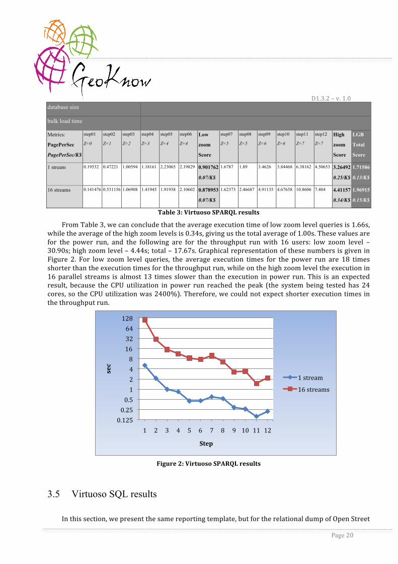
3.4 Virtuoso SPARQL results

In the previous deliverable D1.3.1 (GeoKnow Consortium, 2013), we presented the template that contains all the relevant metrics. In this section, we give the results of benchmark run over RDF data loaded in Virtuoso on a cluster of computers (Table 3). Virtuoso was run in cluster mode where one logical database (with Linked Geodata) is served by a collection of server processes (in our case, there was 4 of them) spread over a cluster of machines (2 machines).

The benchmark tested how the system behaves when it handles one user at a time (power run -‐ 1 stream row), of 16 users for the throughput run (16 streams row). It calculates how many queries can be finish per second (PagePerSec), and it reports this number divided by the dollar cost of the system being tested (PagePerSec/K$). These metrics are measured separately for each step (1-‐12) from the query workload for different zoom levels. The geometric mean of metrics stored in columns from step01 to step06 is written in the column Low zoom score, providing us information of the liability of the system to cope with low zoom level queries. Similarly, the high zoom score is reported, as well as the total score.

FacetBench 1.0 (SF=1)

hardware 2x (dual Xeon E5-2630, 2.33GHz, 192GB RAM, 8 disks)

Software Virtuoso v7

Linux 2.6

Price $13.000 @ November 23, 2013

D1.3.2 – v. 1.0

database size

bulk load time

Metrics:

PagePerSec

PagePerSec/K$

step01

Z=0

step02

Z=1

step03

Z=2

step04

Z=3

step05

Z=4

step06

Z=4

Low

zoom

Score

step07

Z=5

step08

Z=5

step09

Z=6

step10

Z=6

step11

Z=7

step12

Z=7

High

zoom

Score

LGB

Total

Score

1 stream 0.19532

0.47221 1.00594 1.18161 2.23065 2.19829 0.901762

0.07/K$

1.6787

1.89

3.4626

3.84468

6.38162

4.50653

3.26492

0.25/K$

1.71586

0.13/K$

16 streams 0.141476

0.531156

1.06908

1.41945

1.91938

2.10602

0.878953

0.07/K$

1.62373

2.46687 4.91135

4.67658

10.8606

7.404

4.41157

0.34/K$

1.96915

0.15/K$

Table 3: Virtuoso SPARQL results

From Table 3, we can conclude that the average execution time of low zoom level queries is 1.66s, while the average of the high zoom levels is 0.34s, giving us the total average of 1.00s. These values are for the power run, and the following are for the throughput run with 16 users: low zoom level – 30.90s; high zoom level – 4.44s; total – 17.67s. Graphical representation of these numbers is given in Figure 2. For low zoom level queries, the average execution times for the power run are 18 times shorter than the execution times for the throughput run, while on the high zoom level the execution in 16 parallel streams is almost 13 times slower than the execution in power run. This is an expected result, because the CPU utilization in power run reached the peak (the system being tested has 24 cores, so the CPU utilization was 2400%). Therefore, we could not expect shorter execution times in the throughput run.

Figure 2: Virtuoso SPARQL results

3.5 Virtuoso SQL results

In this section, we present the same reporting template, but for the relational dump of Open Street

0.125 0.25 0.5 1 2 4 8 16 32 64 128

1 2 3 4 5 6 7 8 9 10 11 12

sec

Step

1 stream

16 streams

D1.3.2 – v. 1.0

Map with 1.3G nodes. Here, we used the single Virtuoso instance, as well as the cluster configuration.

The results for single instance are in the following Table 4:




Linux 2.6

Price $13.000 @ November 23, 2013

database size

bulk load time

Metrics:

PagePerSec

PagePerSec/K$

step01

Z=0

step02

Z=1

step03

Z=2

step04

Z=3

step05

Z=4

step06

Z=4

Low

zoom

Score

step07

Z=5

step08

Z=5

step09

Z=6

step10

Z=6

step11

Z=7

step12

Z=7

High

zoom

Score

LGB

Total

Score

1 stream 0.0529207

0.0921005 0.203413 0.505894 0.927902 0.956663 0.276474

0.02/K$

2.02634

2.03004

5.71102

4.36872

13.7174

8.81834

4.80896

0.37/K$

1.15306

0.09/K$

16 streams 0.243775

0.360965

0.78531

2.01543

4.45029

4.52088

1.18727

0.09/K$

10.4645

10.7674 32.2244

25.8124

87.8918

54.6322

27.6458

2.13/K$

5.72914

0.44/K$

Table 4: Virtuoso SQL Results (single instance)

In the power run, the average execution time of low zoom level queries is 6.46s. But, for the high zoom levels, the average is lower, as expected: 0.26s. The total average time in the power run is 3.36s. In the throughput run the average values for low zoom level queries, high zoom level queries, and the total average are 24.23s, 0.77s and 12.50s, respectively. The queries running in isolation executed more than 3 times faster. This is an expected result, as well, because the CPU utilization in power run was not so high. These values are shown in the Figure 3.

D1.3.2 – v. 1.0

Figure 3: Virtuoso SQL Results (single instance)

Latter in this chapter, we present the results of the same benchmark, but running Virtuoso in cluster mode (4 processes, 2 machines). The reporting template is shown on the Table 5.




Linux 2.6

Price $13.000 @ November 23, 2013

database size

bulk load time

Metrics:

PagePerSec

PagePerSec/K$

step01

Z=0

step02

Z=1

step03

Z=2

step04

Z=3

step05

Z=4

step06

Z=4

Low

zoom

Score

step07

Z=5

step08

Z=5

step09

Z=6

step10

Z=6

step11

Z=7

step12

Z=7

High

zoom

Score

LGB

Total

Score

1 stream 0.631473

1.42531 4.32713 8.96861 15.3139 14.245 4.43334

0.34/K$

21.1416

22.4719

56.4972

50.5051

100

78.7402

46.8512

3.60/K$

14.4121

1.11/K$

16 streams 1.92231

3.21515

4.77236

7.49611

12.4098

12.818

5.71997

0.44/K$

24.4641

25.5404 67.2199

56.166

138.739

95.5892

56.0432

4.31/K$

17.9043

1.38/K$

Table 5: Virtuoso SQL Results (cluster)

In the power run, the average execution time of low level queries, high level queries and the total average are 0.46s, 0.03, and 0.24s, respectively, while in the throughput run these numbers are: 3.55s, 0.35, and 1.95. This is about 8 times slower. All of these values are graphically presented in the Figure

0.0625 0.125 0.25 0.5 1 2 4 8 16 32 64 128

1 2 3 4 5 6 7 8 9 10 11 12

sec

Step

1 stream

16 streams

D1.3.2 – v. 1.0

4.

Figure 4: Virtuoso SQL Results (cluster)

3.6 PostGIS SQL results

In this section, we give the benchmark results of PostGIS in SQL as a point of reference. The dataset being tested is almost the same as the dataset in question in the previous section. The reporting template is shown in the Table 6.


hardware 2x (dual Xeon E5-2630, 2.33GHz, 192GB RAM, SSD)

Software PostgreSQL 9.1 with PostGIS 1.5.8

Linux 2.6

Price $13.000 @ November 23, 2013

database size

bulk load time

Metrics:

PagePerSec

PagePerSec/K$

step01

Z=0

step02

Z=1

step03

Z=2

step04

Z=3

step05

Z=4

step06

Z=4

Low

zoom

Score

step07

Z=5

step08

Z=5

step09

Z=6

step10

Z=6

step11

Z=7

step12

Z=7

High

zoom

Score

LGB

Total

Score

1 stream 0.00109

0.00589 0.01194 0.01681 0.02321 0.24638 0.00952

0.0007/K$

0.05367

0.06179

0.17985

0.18241

1.53304

1.069

0.23738

0.0183/K$

0.04754

0.0037/K$

16 streams 0.00964

0.04613

0.11510

0.19664

0.29607

0.30318

0.09842

0.0076/K$

0.74051

0.75399 5.28043

4.3347

23.3231

15.166

4.06399

0.3126/K$

0.63242

0.0486/K$

0.0078125 0.015625 0.03125 0.0625 0.125 0.25 0.5 1 2 4 8 16

1 2 3 4 5 6 7 8 9 10 11 12

sec

Step

1 stream

16 streams

D1.3.2 – v. 1.0

Table 6: PostGIS results

In the power run, the average execution times of low zoom level queries, high zoom level queries, and total average are 218.96s, 7.91s and 113.43s, respectively. In the throughput run related numbers are only slightly higher (from 8% to 77%): 388.94s, 8.55s and 198.75s. This ratio is reasonable because the CPU utilization in power run in this case was so low. Figure 5 contains a graph of the average execution time of each step in the workload.

Figure 5: PostGIS results

3.7 Results Comparison

In this section, we summarize the results collected in the preceding ones. We present the comparison of these four systems separately on the power run, and on the throughput run.

In Figure 6 the power run comparison is presented. Virtuoso in both SQL and SPARQL outperformed PostGIS by large factor. Specifically, all the queries in the power run were executed 33 times slower in PostGIS than in Virtuoso SQL (single server). If we compare PostGIS with Virtuoso SPARQL, the factor will be even greater: 131 for low zoom level queries, 23 for high zoom level queries, and 113 in total. If we correlate Virtuoso SPARQL and SQL (single server), we will conclude that the relational version is slower almost 4 times on low zoom level queries, while it is faster 23% on high zoom level. In total, SQL version is slower more than 3 times. But, if we compare Virtuoso SPARQL and SQL, but with cluster configuration, we will conclude that SQL is faster more than 3 times on low zoom level, more than 13 times on high zoom level, and more than 4 times in total. Therefore, the largest factor is between PostGIS and Virtuoso SQL with cluster setting (more than 466).

0.5 1 2 4 8 16 32 64 128 256 512 1024 2048

1 2 3 4 5 6 7 8 9 10 11 12

sec

Step

1 stream

16 streams

D1.3.2 – v. 1.0

Figure 6: Power Run Comparison

In Figure 7 the throughput run comparison is shown. Virtuoso in both variants outperformed PostGIS but not with a huge factor as in the previous case. On low zoom levels, the factor was more than 16 for SQL version (single server), and 12.6 for SPARQL version; on high zoom levels, it was 11 for SQL (single), but for SPARQL it was almost 2. From Figure 7, it is obvious that PostGIS was slightly faster than Virtuoso SPARQL on the highest zoom level. Taking into account all steps from workload, PostGIS was slower almost 16 times than Virtuoso SQL (single server), and more than 11 times than Virtuoso SPARQL. Comparing Virtuoso versions, on low zoom level queries SQL version (single server) was 22% faster, while on high zoom levels it was faster almost 6 times. In total, SQL version (single server) is faster 30%. Virtuoso running on cluster was 6 times faster than running on single server, while more than 100 times faster comparing with PostGIS.

Analyzing these results, one should bear in mind that Virtuoso SPARQL was tested only a cluster of computers.

Figure 7: Throughput Run Comparison

0.0078125

0.03125

0.125

0.5

2

8

32

128

512

1 2 3 4 5 6 7 8 9 10 11 12

sec

Step

Virtuoso SPARQL

Virtuoso SQL

PostGIS SQL

Virtuoso SQL cluster

0.0625

0.25

1

4

16

64

256

1024

1 2 3 4 5 6 7 8 9 10 11 12

sec

Step

Virtuoso SPARQL

Virtuoso SQL

PostGIS SQL

Virtuoso SQL cluster

D1.3.2 – v. 1.0

D1.3.2 – v. 1.0

4. Query Plans

One of the reasons why PostGIS is much slower than Virtuoso, is the query planner.

4.1 PostGIS Query Plans

For the most queries, PostGIS query planner did not choose the optional query plan, thus the average execution times are bad while comparing with Virtuoso results. Let us take for example the facet count query: EXPLAIN ANALYZE select t.type, count(*) as cnt from nodes as n, node_types as t where n.id=t.node_id and ST_Intersects(geom, ST_MakeEnvelope(LONGITUDE-WIDTH/2, LATITUDE-HEIGHT/2, LONGITUDE+WIDTH/2, LATITUDE+HEIGHT/2, 4326)) group by t.type order by cnt desc limit 50

Almost all the facet count queries have the query plan stated in the Appendix 8.1. Exceptions are the queries from the highest zoom level. In the problematic query plan, we have a hash join of the tables nodes and node_types, where in the “build” phase of the algorithm, the hash table of the relation nodes is prepared (build), and the relation node_types is scanned in sequence (probe). This is wrong, because the relation nodes is larger one. The average execution time of these queries on the lowest zoom level is about 1000s.

If we disable the query planner's use of hash-‐join plan types with SET enable_hashjoin = false;

that is by default on, we will have a merge join instead. In this case, the execution will be 20% faster, but even then, Virtuoso will be significantly faster.

If we disable the use of merge-‐join plan types, as well, with SET enable_mergejoin = false;

we will have a nested loop instead. This will bring a slight improvement in execution time, comparing with merge join.

Queries from the highest zoom level have the correct query plan (Appendix 8.1). Here, we have a nested loop, and use of geo index over nodes. This leads to the comparable execution times, noticeable in every figure and table from sections 3.6 and 3.7.

This analysis is exactly the same for all other queries (instance queries and instance aggregation queries).

D1.3.2 – v. 1.0

5. Grid Division

This task divides the globe into squares of so many fractions of a degree on the side in such a way that no square contains more than a set number of points. The initial setting is a 30x30 division into squares of 12 degrees on the side. The process is iterative, dividing each square into 4 equal (in terms of angle) squares if the square has more points than the set limit.

The task accesses the totality of the geodata in the system and has high demand for throughput but is only moderately sensitive to latency.

The main query on each iteration is: insert into geo_stat (gs_sq_id, gs_geo, gs_cnt)

select sq_id, sq_geo, count (*)

from geo_square, rdf_quad

where sq_status = 1 and st_intersects (sq_geo, o)

group by sq_id

having count (*) > grain option (order);

This is a spatial join between the squares that had more than the desired count and the totality of the RDF geometries, so that all geometries intersecting the square are retrieved and grouped by the id of the square. Only those squares that have over the count are returned for processing on the next iteration. The algorithm stops when all squares are below the count. The access pattern is a drill down in all densely populated locations at the same time.

The task is first run with cold geo index. The cluster status summary for, before, and after can be found in Appendix 8.2.

The first pass is repeated with warm cache below, followed by the whole run. The world is split into squares until no square has over 20000 points. After each iteration, the count of squares with over 20000 points, as well as the total number of points within these squares is given.

We note that each geometry point is counted twice since it occurs in the object position of a triple twice: Once for the geometry and once for the denormalization where the node directly refers to its geometry.

At intervals we show the cluster status summary with CPU and interconnect utilization. This is not repeated for all points. We note that as soon as the working set is in memory there is near perfect platform utilization. For the first few iterations, the number of points does not decrease and the run time increases slightly. This is because the number of distinct squares, hence of distinct geo lookup keys increases, i.e. more lookups retrieve the same number of points. The increase is small though as vectoring and other techniques absorb the overhead. After this the times start dropping as the number of squares with over 20000 points and their share of the total point population starts dropping. Here we see the selective part of the geo lookups.

At the end of dividing, the following query summarizes the task: select top 100 floor (log (st_area (sq_geo)) )as a, count (*)

D1.3.2 – v. 1.0

from geo_square

group by a

order by 2;

a aggregate

INTEGER INTEGER NOT NULL

_______________________________________________________________________________

-13 4

-14 16

3 336

-12 347

4 626

2 966

0 3548

-1 9095

-2 19499

-11 20272

-4 45051

-9 59074

-8 96539

-5 97976

-7 144831

After this each point belongs to exactly one grid square. The grid square can be efficiently determined given the point by a lookup in a small R tree. The count of distinct squares is at most in the millions, hence the squares themselves can be easily replicated on all nodes of a scale out system.

D1.3.2 – v. 1.0

6. Analytical Queries

In order to make informed business decisions, there is a need to turn the data in corporate database into useful information. The following BI queries demonstrate this. Queries touching large fractions of the data are primarily useful for checking consistency and high level data summarization. Business intelligence analytics in this context would be more scoped, to specific countries and rural and urban areas, for example.

We begin with data summarization questions and comparisons between datasets:

• Q1: For each country, show the total count of features in Dbpedia, Geonames and OSM. sparql select ?cname (sum(if (?g_graph = <lgd_ext>, 1, 0)) as ?n_lgd) (sum(if (?g_graph = <http://dbpedia.org>, 1, 0)) as ?n_dbp) (sum(if (?g_graph != <http://dbpedia.org> && ?g_graph != <lgd_ext> && ?g_graph != <sqs>, 1, 0)) as ?n_geo) where { graph ?g_graph { ?feature geo:geometry ?sgeo . } . ?sq geo:geometry ?sqgeo . filter (bif:st_intersects (?sqgeo, ?sgeo)) ?sq <sq-belongs-to-country> ?country . ?country <http://www.geonames.org/ontology#name> ?cname } group by ?cname order by desc 2

• Q2: For each country, show the count of offers (amenities for sale), with the total price sorted by the count of them. sparql select ?country, count(1), sum (?sale_price) where { ?offer a <http://linkedgeodata.org/ontology/Offer> ; <http://linkedgeodata.org/ontology/subject> ?re_subj ; <http://linkedgeodata.org/ontology/sale_price> ?sale_price . ?re_subj geo:geometry ?sgeo . ?sq geo:geometry ?sqgeo . filter (bif:st_intersects (?sqgeo, ?sgeo)) ?sq <sq-belongs-to-country> ?country . } group by ?country order by desc 2 For this, sale events are generated so that an amenity has a 1/20 chance of being for sale in each of the 10 past years, i.e. there is a 1/2 chance that an amenity has been for sale in the past decade. A surface area is randomly chosen between 100 and 1000. The price is

D1.3.2 – v. 1.0

±50% of a country dependent average with being in 20 km of a city doubles the price.

• Q3: Count of all features and count of features that belong to some country sparql select count (*) count (?country) where { ?feature geo:geometry ?sgeo . graph <sqs> { ?sq geo:geometry ?sqgeo . } . filter (bif:st_intersects (?sqgeo, ?sgeo)) . optional { ?sq <sq-belongs-to-country> ?country . } }

The execution times of these queries are listed in the Table 7.

Query name Time in ms

Q1 200764

Q2 131916

Q3 364100 Table 7: BI Query Results

The results, execution times and query plans of the previous queries can be found in the Appendix 8.3. Some similar BI queries could be:

• What is the ratio of the count of points within 10 km of a city center over all the points in the world?

• As above, except now we count the unique points within 10km of any city center in the country of the point and divide by the total number of points in the country. Group by country, sort by highest percentage first. Note that there can be points that are within 10km of more than one city center.

• List countries ranked by the count of points divided by the population. Where are the most active contributions?

• Return the top 100 squares with the highest price of retail space per square meter for countries in a region.

6.1 Producing DXF

The most convenient format of the results of these queries is not textual. It would be useful if the results can be displayed on a map. In this section, we present a way of doing it.

Drawing exchange format (DXF) is a file format for graphics information, for enabling data interoperability between AutoCAD and other programs. It is an ASME/ANSI standard that is used for PC-‐based CAD/CAM platforms. DXF enables vector data exchange as well as 2D and 3D graphics drawing.

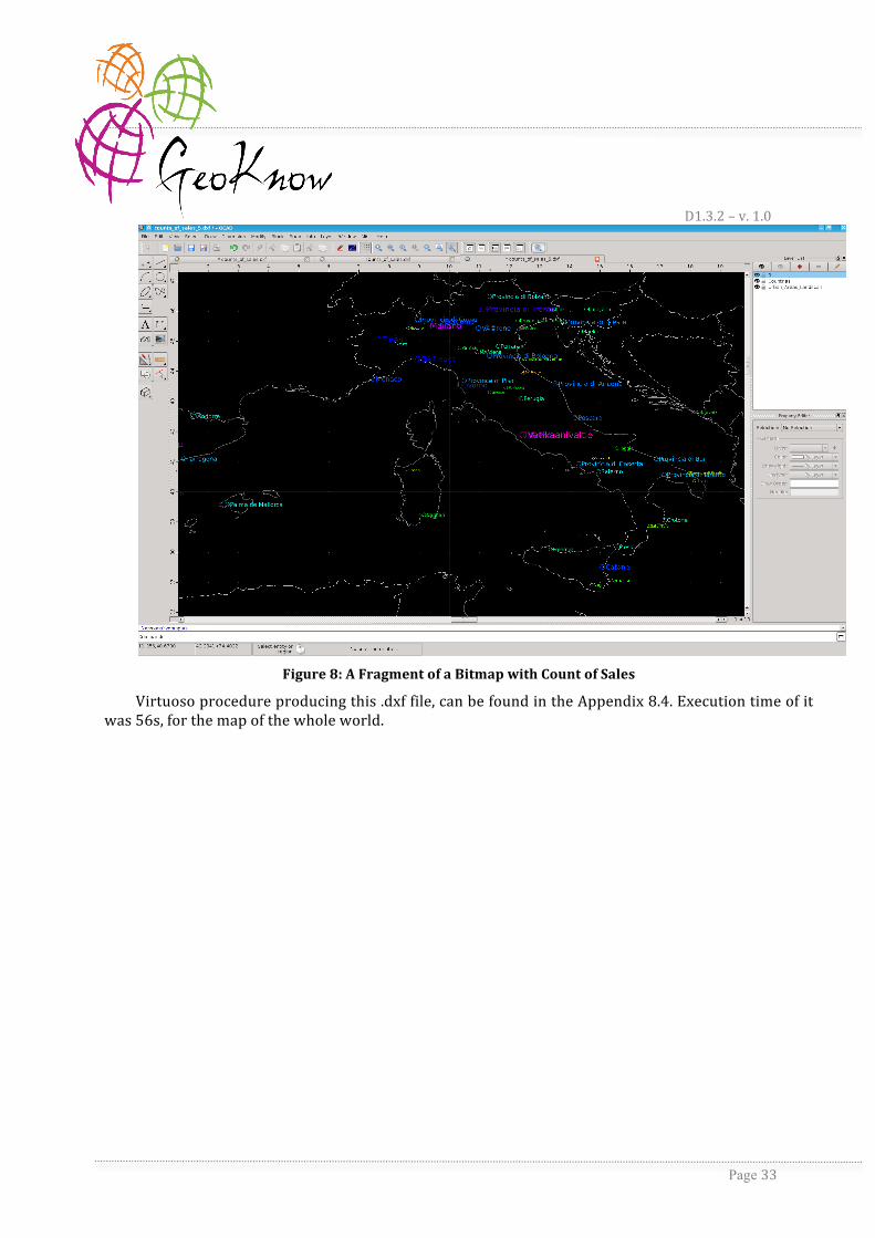
Here, we detail the Virtuoso procedure that will produce the .dxf file, containing a map with the integrated features requested by BI query. For example, we consider the following query:

select ?city, <sql:BEST_LANGMATCH>(?cityoname,

D1.3.2 – v. 1.0

"en-gb;q=0.8, en;q=0.7, fr;q=0.6, *;q=0.1", "") as ?city_official_name,

count(1) as ?sales_count,

avg(?re_subj_lat) as ?avg_lat, avg (?re_subj_long) as ?avg_long

where {

?offer a <http://linkedgeodata.org/ontology/Offer> ;

<http://linkedgeodata.org/ontology/subject> ?re_subj ;

<http://linkedgeodata.org/ontology/sale_price> ?sale_price .

?re_subj geo:lat ?re_subj_lat ; geo:long ?re_subj_long .

graph <sq-city> { ?sq <sq-belongs-to-city> ?city }

filter (?sq =

<(NUM,NUM)SHORT::sql:xy_square_iid> (?re_subj_long, ?re_subj_lat))

?city <http://www.geonames.org/ontology#officialName> ?cityoname

}

group by ?city

This query summarizes the offers per city (count of them), and returns the average latitude and longitude of them. If we export the results of the query to the .dxf file, a fragment of a bitmap rendered by software dealing with this kind of files could be as shown in the Figure 8. Colors and sizes of the cities are chosen depending on the count of the offers in the city in question.

D1.3.2 – v. 1.0

Figure 8: A Fragment of a Bitmap with Count of Sales

Virtuoso procedure producing this .dxf file, can be found in the Appendix 8.4. Execution time of it was 56s, for the map of the whole world.

D1.3.2 – v. 1.0

7. Conclusion

In this deliverable, we presented an update of the configuration of the GeoKnow Benchmarking System. We improved the benchmark and expanded it to be used for relational data, as well. The migration procedure of OSM data from PostGIS to Virtuoso is improved. We used this Benchmarking System to evaluate the performance of the different RDF stores, and the RDBMS’es (Virtuoso and PostGIS), and to compare the results between them. We presented PostGIS query plans, as one of the possible reasons why PostGIS is much slower than Virtuoso. The grid division task is specified, as a new idea of how a scale out system can be improved. The BI queries are specified, developed, and measured, as well as a way of producing the .dxf file from the results of the queries.

D1.3.2 – v. 1.0

8. Appendix

All the scripts and programs from the GeoKnow Benchmark are available as a git project: https://github.com/GeoKnow/GeoBenchLab

The current version of the migration scripts that transfers the OSM data from PostgreSQL to Virtuoso are available here:

https://dl.dropboxusercontent.com/u/27316106/migration.tar.gz

8.1 PostGIS query plans

Query plan of all the facet count queries (except queries from the highest zoom level): Limit (cost=47835546.24..47835546.37 rows=50 width=101) (actual time=1125920.197..1125920.210

rows=50 loops=1)

-> Sort (cost=47835546.24..47835547.30 rows=423 width=101) (actual time=1125920.195..1125920.200 rows=50 loops=1)

Sort Key: (count(*))

Sort Method: top-N heapsort Memory: 32kB

-> HashAggregate (cost=47835527.96..47835532.19 rows=423 width=101) (actual time=1125919.583..1125919.780 rows=909 loops=1)

-> Hash Join (cost=44785326.16..47831863.32 rows=732929 width=101) (actual time=1026163.888..1124232.847 rows=2311400 loops=1)

Hash Cond: (t.node_id = n.id)

-> Seq Scan on node_types t (cost=0.00..761033.86 rows=27936686 width=109) (actual time=0.010..12868.866 rows=27936634 loops=1)

-> Hash (cost=44246225.23..44246225.23 rows=32859434 width=8) (actual time=1024822.421..1024822.421 rows=96122281 loops=1)

Buckets: 4096 Batches: 4096 (originally 2048) Memory Usage: 1025kB

-> Bitmap Heap Scan on nodes n (cost=3137472.07..44246225.23 rows=32859434 width=8) (actual time=238660.910..972205.201 rows=96122281 loops=1)

Recheck Cond: (geom && '0103000020E610000001000000050000001361C3D32B6599BF6688635DDCD648401361C3D32B6599BF6688635DDC164B404F1E166A4DF321406688635DDC164B404F1E166A4DF321406688635DDCD648401361C3D32B6599BF6688635DDCD64840'::geometry)

Filter: _st_intersects(geom, '0103000020E610000001000000050000001361C3D32B6599BF6688635DDCD648401361C3D32B6599BF6688635DDC164B404F1E166A4DF321406688635DDC164B404F1E166A4DF321406688635DDCD648401361C3D32B6599BF6688635DDCD64840'::geometry)

-> Bitmap Index Scan on idx_nodes_geom (cost=0.00..3129257.21 rows=98578313 width=0) (actual time=238636.331..238636.331 rows=96147748 loops=1)

Index Cond: (geom && '0103000020E610000001000000050000001361C3D32B6599BF6688635DDCD648401361C3D32B6599BF6688635DDC164B404F1E166A4DF321406688635DDC164B404F1E166A4DF321406688635DDCD648401361C3D32B6599BF6688635DDCD64840'::ge

D1.3.2 – v. 1.0

ometry)

Query plan of the facet count queries from the highest zoom level: Limit (cost=424622.60..424622.73 rows=50 width=101) (actual time=393.969..393.981 rows=50

loops=1)

-> Sort (cost=424622.60..424622.93 rows=133 width=101) (actual time=393.968..393.973 rows=50 loops=1)

Sort Key: (count(*))

Sort Method: quicksort Memory: 37kB

-> HashAggregate (cost=424616.85..424618.18 rows=133 width=101) (actual time=393.865..393.882 rows=89 loops=1)

-> Nested Loop (cost=0.00..424616.19 rows=133 width=101) (actual time=2.215..392.729 rows=1232 loops=1)

-> Index Scan using idx_nodes_geom on nodes n (cost=0.00..76852.86 rows=5948 width=8) (actual time=0.415..124.744 rows=29344 loops=1)

Index Cond: (geom && '0103000020E6100000010000000500000034BA83D899C211408048BF7D1DF0494034BA83D899C21140F853E3A59BF449400ABFD4CF9B0A1240F853E3A59BF449400ABFD4CF9B0A12408048BF7D1DF0494034BA83D899C211408048BF7D1DF04940'::geometry)

Filter: _st_intersects(geom, '0103000020E6100000010000000500000034BA83D899C211408048BF7D1DF0494034BA83D899C21140F853E3A59BF449400ABFD4CF9B0A1240F853E3A59BF449400ABFD4CF9B0A12408048BF7D1DF0494034BA83D899C211408048BF7D1DF04940'::geometry)

-> Index Scan using pk_node_types on node_types t (cost=0.00..58.25 rows=17 width=109) (actual time=0.009..0.009 rows=0 loops=29344)

Index Cond: (node_id = n.id)

8.2 Grid Division

Cluster 4 nodes, 1285 s. 11 m/s 3 KB/s 666% cpu 496% read 0% clw threads 1r 0w 0i buffers 12974829 206 d 0 w 2 pfs

cl 1: 5 m/s 2 KB/s 129% cpu 204% read 0% clw threads 1r 0w 0i buffers 3269072 38 d 0 w 2 pfs




Iter 1 -- 219713 msec.






select count (*), sum (gs_cnt) from geo_stat where gs_cnt > 10000;

274 3998898331

iTER 2 Done. -- 218499 msec.

760 3997850489

D1.3.2 – v. 1.0

Iter 3 . -- 223179 msec.

2074 3992914437

Iter 4 Done. -- 227770 msec.

4748 3969470524


9897 3905745538

Iter 6 . -- 262611 msec.

20089 375759190


35305 3381997920

Done. -- 308270 msec.






43244 2523650520


28145 1322847177


16041 592433083







5090 141521188


88 2052076


5 105737


0 0

D1.3.2 – v. 1.0

8.3 Execution of the Analytical Queries profile ('

sparql select ?country, count(1), sum (?sale_price)

where

{




?re_subj geo:geometry ?sgeo .

?sq geo:geometry ?sqgeo .

filter (bif:st_intersects (?sqgeo, ?sgeo))

?sq <sq-belongs-to-country> ?country .

} group by ?country order by desc 2

');

result

LONG VARCHAR

_______________________________________________________________________________

http://sws.geonames.org/3077311/ 103580 121039191590








http://sws.geonames.org/2077456/ 6169 -4285350253












D1.3.2 – v. 1.0

{

time 5.6e-08% fanout 1 input 1 rows

time 0.0021% fanout 1 input 1 rows

{ hash filler

wait time 0% of exec real time, fanout 0

QF {


Stage 1

time 0.0007% fanout 21798.7 input 48 rows

RDF_QUAD 1.1e+06 rows(s_13_12_t1.O, s_13_12_t1.S)

inlined P = #/subject

time 0.18% fanout 3.44745 input 1.04634e+06 rows

Stage 2

time 0.0044% fanout 0 input 4.18535e+06 rows

Sort hf 39 replicated(s_13_12_t1.O) -> (s_13_12_t1.S)

}

}

Subquery 45

{


{ fork


{ fork

wait time 2.2e-09% of exec real time, fanout 0

QF {


Stage 1


RDF_QUAD 2.4e+05 rows(s_13_12_t5.S, s_13_12_t5.O)

inlined P = #Â¶sq-belongs-to-country


END Node

After test:

0: if ( 0 = 1 ) then 5 else 4 unkn 5

4: BReturn 1

5: BReturn 0


RDF_QUAD 1 rows(s_13_12_t4.O)

inlined P = ##geometry , S = k_s_13_12_t5.S


D1.3.2 – v. 1.0

Precode:

0: QNode {

time 0% fanout 0 input 0 rows

dpipe

s_13_12_t4.O -> __RO2SQ -> __ro2sq

}

2: BReturn 0

Stage 2

time 64% fanout 85.3929 input 1.18754e+07 rows

geo 3 st_intersects (__ro2sq) node on DB.DBA.RDF_GEO 0 rows

s_13_12_t3.O


RDF_QUAD_POGS 2 rows(s_13_12_t3.S)

P = ##geometry , O = cast

hash partition+bloom by 43 ()

time 5.2% fanout 0.000434695 input 1.01387e+09 rows

Hash source 39 1.7 rows(cast) -> (s_13_12_t1.S)


Stage 3


RDF_QUAD 1.1 rows(s_13_12_t2.S, s_13_12_t2.O)

inlined P = #/sale_price , S = q_s_13_12_t1.S


RDF_QUAD 0.8 rows()

inlined P = ##type , S = k_q_s_13_12_t1.S , O = #/Offer


Sort (set_no, s_13_12_t5.O) -> (s_13_12_t2.O, inc)

}

}


group by read node

(gb_set_no, s_13_12_t5.O, aggregate, aggregate)


Sort (aggregate) -> (s_13_12_t5.O, aggregate)

}


Key from temp (s_13_12_t5.O, aggregate, aggregate)

D1.3.2 – v. 1.0

After code:

0: QNode {


dpipe

s_13_12_t5.O -> __RO2SQ -> __ro2sq

}

2: callret-1 := := artm aggregate


10: country := := artm __ro2sq

14: BReturn 0


Subquery Select(country, callret-1, callret-2)

}

After code:

0: QNode {


dpipe

s_13_12_t5.O -> __RO2SQ -> __ro2sq

}



10: country := := artm __ro2sq

14: BReturn 0


Subquery Select(country, callret-1, callret-2)

}

After code:

0: QNode {


dpipe

callret-2 -> __RO2SQ -> callret-2

callret-1 -> __RO2SQ -> callret-1

country -> __RO2SQ -> country

}

D1.3.2 – v. 1.0

2: BReturn 0


Select (country, callret-1, callret-2)

}

131916 msec 3860% cpu, 1.0153e+09 rnd 4.16182e+10 seq 99.699% same seg 0.281927% same pg

633 disk reads, 0 read ahead, 0.119788% wait

42977 messages 13581 bytes/m, 0.0078% clw

Compilation: 4 msec 0 reads 0% read 0 messages 0% clw

CPU: Intel Sandy Bridge microarchitecture, speed 2299.98 MHz (estimated)

Counted CPU_CLK_UNHALTED events (Clock cycles when not halted) with a unit mask of 0x00 (No unit mask) count 100000

samples % symbol name

19335499 31.9950 cmpf_geo

12022031 19.8932 itc_page_search

3860950 6.3888 dv_compare

3370690 5.5776 dc_any_cmp

2833115 4.6880 itc_param_cmp

2184864 3.6154 hash_source_chash_input

1728851 2.8608 gen_qsort

1383613 2.2895 cs_decode

1198923 1.9839 box_to_any_1

669706 1.1082 itc_next

667466 1.1045 page_find_leaf

478367 0.7916 ce_result

472240 0.7814 dc_append_bytes

profile ('

sparql select ?cname

(sum(if (?g_graph = <lgd_ext>, 1, 0)) as ?n_lgd)

(sum(if (?g_graph = <http://dbpedia.org>, 1, 0)) as ?n_dbp)

(sum(if (?g_graph != <http://dbpedia.org> && ?g_graph != <lgd_ext> && ?g_graph != <sqs>, 1, 0)) as ?n_geo)

where

{

graph ?g_graph { ?feature geo:geometry ?sgeo . } .

?sq geo:geometry ?sqgeo .

filter (bif:st_intersects (?sqgeo, ?sgeo))

D1.3.2 – v. 1.0

?sq <sq-belongs-to-country> ?country .

?country <http://www.geonames.org/ontology#name> ?cname

} group by ?cname order by desc 2

');

United Kingdom of Great Britain and Northern Ireland 361739459 133784 516810

Czech Republic 141304028 25122 180744

Japan 88147723 13342 37289

Repubblica Italiana 77138844 13073 46984

Kingdom of Norway 51099745 7182 21254

Republic of Austria 29263512 1692 44605

Republic of Suriname 17671910 4924 84530

Commonwealth of Australia 17325308 19531 166792

Canada 16661337 6508 22338

Taiwan 14649920 2231 33687

Plurinational State of Bolivia 13617794 7054 103531

Dominica 11907956 1581 12762

Republic of France 11508495 1899 63185

Republic of Chile 11187920 8733 300017

Kingdom of Tonga 10447980 4376 62762

Federal Democratic Republic of Nepal 10228427 5417 46208

Republic of Indonesia 9684176 1514 311943

Ireland 6250504 3748 21269

Portuguese Republic 6224670 2408 27947

New Zealand 5933053 1874 73332

{


Subquery 27

{


{ fork


{ fork


QF {


Stage 1


D1.3.2 – v. 1.0

RDF_QUAD 2.4e+05 rows(s_15_8_t2.S, s_15_8_t2.O)



END Node

After test:

0: if ( 0 = 1 ) then 5 else 4 unkn 5

4: BReturn 1

5: BReturn 0



inlined P = ##geometry , S = k_s_15_8_t2.S

time 24% fanout 0.527002 input 247405 rows

Precode:

0: QNode {


dpipe

s_15_8_t1.O -> __RO2SQ -> __ro2sq

}

2: BReturn 0

Stage 2



inlined P = ##name , S = q_s_15_8_t2.O


Stage 3



s_7_1_t0.O


RDF_QUAD_POGS 2 rows(s_7_1_t0.G)


After code:

0: neq := Call neq (s_7_1_t0.G, #/dbpedia.org )

5: neq := Call neq (s_7_1_t0.G, #Â¶lgd_ext )

10: __and := Call __and (neq, neq)

15: neq := Call neq (s_7_1_t0.G, #Â¶sqs )

20: __and := Call __and (__and, neq)

25: if (__and = 0 ) then 29 else 34 unkn 34

D1.3.2 – v. 1.0

29: callretSimpleCASE := := artm 0

33: Jump 38 (level=0)


38: equ := Call equ (s_7_1_t0.G, #/dbpedia.org )

43: if (equ = 0 ) then 47 else 52 unkn 52




56: equ := Call equ (s_7_1_t0.G, #Â¶lgd_ext )

61: if (equ = 0 ) then 65 else 70 unkn 70




74: BReturn 0

time 1.3% fanout 0 input 1.01387e+09 rows

Sort (s_15_8_t3.O) -> (callretSimpleCASE, callretSimpleCASE, callretSimpleCASE)

}

}


group by read node

(s_15_8_t3.O, aggregate, aggregate, aggregate)


Sort (aggregate) -> (s_15_8_t3.O, aggregate, aggregate)

}

}


group by read node

(s_15_8_t3.O, aggregate, aggregate, aggregate)


Sort (aggregate) -> (s_15_8_t3.O, aggregate, aggregate)

}

time 2e-05% fanout 107 input 1 rows

Key from temp (s_15_8_t3.O, aggregate, aggregate, aggregate)

After code:

0: QNode {


D1.3.2 – v. 1.0

dpipe

s_15_8_t3.O -> __RO2SQ -> __ro2sq

}

2: n_lgd := := artm aggregate

6: n_dbp := := artm aggregate

10: n_geo := := artm aggregate

14: cname := := artm __ro2sq

18: BReturn 0


Subquery Select(cname, n_lgd, n_dbp, n_geo)

}

After code:

0: QNode {


dpipe

n_geo -> __RO2SQ -> n_geo

n_dbp -> __RO2SQ -> n_dbp

n_lgd -> __RO2SQ -> n_lgd

cname -> __RO2SQ -> cname

}

2: BReturn 0


Select (cname, n_lgd, n_dbp, n_geo)

}




profile ('

sparql select count (*) count (?country)

where {

?feature geo:geometry ?sgeo .

graph <sqs> { ?sq geo:geometry ?sqgeo . } .

filter (bif:st_intersects (?sqgeo, ?sgeo)) .

D1.3.2 – v. 1.0

optional { ?sq <sq-belongs-to-country> ?country . }

}');

2010826982 1013872046

{



{ hash filler


QF {


Stage 1


RDF_QUAD_POGS 2.5e+05 rows(t4.S, t4.O)



Stage 2


Sort hf 39 replicated(t4.S) -> (t4.O)

}

}


{ fork


QF {


RDF_QUAD_POGS 3.8e+08 rows(t2.S, t2.O)

inlined P = ##geometry G = #Â¶sqs


END Node

After test:

0: if ( 0 = 1 ) then 5 else 4 unkn 5

4: BReturn 1

5: BReturn 0


qf select node output: (qf_set_no, t2.S, t2.O)

}

D1.3.2 – v. 1.0


Precode:

0: QNode {


dpipe

t2.O -> __RO2SQ -> __ro2sq

}

2: BReturn 0

outer {


Hash source 39 1 rows(k_t2.S) -> (t4.O)

time 3.2e-05% fanout 2.01362 input 247405 rows

end of outer}

set_ctr

out: (t4.O)

shadow: (t4.O)


Precode:

0: isnotnull := Call isnotnull (t4.O)

5: BReturn 0

QF {



t1.O

time 57% fanout 0 input 2.00557e+09 rows

RDF_QUAD_POGS 2 rows()


After code:

0: sum callret-1isnotnullset no set_ctr

5: sum callret-0 1 set no set_ctr

10: BReturn 0

}

}


Select (callret-0, callret-1)

}

D1.3.2 – v. 1.0


7766 disk reads, 7213 read ahead, 0.452942% wait



8.4 Virtuoso Procedure for Producing DXF File create procedure lgd_render_amounts_of_sales ()

{

declare ses, ctx any;

ses := string_output ();

DXFOUT_PREAMBLE (ses, ctx);

for (select SHP_SOURCE_IDX, deserialize (SHP_GEOM) as geom from DB.DBA."SHP_NE1_ne_10m_admin_0_countries") do

http_st_dxf_entity (geom, vector (62, 253), ses);

for (

sparql define input:storage "" select ?city,

<sql:BEST_LANGMATCH>(?cityoname, "en-gb;q=0.8, en;q=0.7, fr;q=0.6, *;q=0.1", "") as ?city_official_name,

count(1) as ?sales_count,

avg(?re_subj_lat) as ?avg_lat, avg (?re_subj_long) as ?avg_long where

{




?re_subj geo:lat ?re_subj_lat ; geo:long ?re_subj_long .

graph <sq-city> { ?sq <sq-belongs-to-city> ?city }

filter (?sq = <(NUM,NUM)SHORT::sql:xy_square_iid> (?re_subj_long, ?re_subj_lat))

?city <http://www.geonames.org/ontology#officialName> ?cityoname

} group by ?city) do

{

declare color integer;

declare sz double precision;

color := 10 + 10 * floor (log10("sales_count") * 5.0);

sz := (1+log10("sales_count")) * 0.1;

http_raw_dxf_entity (vector (0, 'TEXT', 1, "city_official_name", 6, 'BYLAYER', 62, color,

10, "avg_long" + 1.5*sz, 20, "avg_lat", 30, 0.0,

11, "avg_long" + 1.5*sz, 21, "avg_lat", 31, 0.0,

40, 2*sz, 41, 1.0, 50, 0.0, 71, 0, 72, 0, 73, 2 ), ses);

http_raw_dxf_entity (vector (0, 'CIRCLE', 6, 'BYLAYER', 62, color, 10, "avg_long", 20, "avg_lat", 40, sz), ses);

}

D1.3.2 – v. 1.0

DXFOUT_CONCLUSION (ses, ctx);

string_to_file ('counts_of_sales.dxf', ses, -2);

}

;

create procedure xy_square_iid (in x any array, in y any array) returns IRI_ID_8

{

vectored;

return (select __i2id (sprintf ('sq%d', sq_id)) from geo_square where st_intersects (sq_geo, st_point (x, y)));

}

;

D1.3.2 – v. 1.0

9. Bibliography Bayer, R. (1971). Binary B-‐trees for Virtual Memory. In Proceedings of the 1971 ACM SIGFIDET

(Now SIGMOD) Workshop on Data Description, Access and Control (pp. 219-‐-‐235). New York, NY, USA: ACM.

GeoKnow Consortium. (2013, 06 18). Design and Setup of Benchmarking System. Retrieved 12 04, 2013, from GeoKnow Deliverables: svn.aksw.org/projects/GeoKnow/Deliverables/D1.3.1/D1.3.1_Design_and_Setup_of_Benchmarking_System.pdf

Guttman, A. (1984). R-‐Trees: A Dynamic Index Structure for Spatial Searching. In B. Yormark, SIGMOD'84, Proceedings of Annual Meeting (pp. 47-‐57). Boston, Massachusetts: ACM Press.

Lod2 Consortium. (2010). Retrieved 12 04, 2013, from Creating Knowledge out of Interlinked Data: http://lod2.eu/Welcome.html

Open Geospatial Consortium. (2012). GeoSPARQL - A Geographic Query Language for RDF Data. Retrieved 12 04, 2013, from http://www.opengeospatial.org/standards/geosparql

OpenStreetMap Project. (n.d.). About OpenStreetMap. Retrieved 12 04, 2013, from OpenStreetMap Web site: http://www.openstreetmap.org/about

OpenStreetMap Project. (2013, 09 08). Osmosis. Retrieved 12 04, 2013, from OpenStreetMap Wiki: http://wiki.openstreetmap.org/wiki/Osmosis

d1.3.2 continuous report on performance evaluation

Documents