d-wave hybrid solver service + advantage: technology update

CONTACT

Corporate Headquarters3033 Beta AveBurnaby, BC V5G 4M9CanadaTel. 604-630-1428

US O�ce2650 E Bayshore RdPalo Alto, CA 94303

Email: [email protected]

www.dwavesys.com

Overview

The D-Wave hybrid solver service (HSS), available from the LeapTM

quantum cloud service, was launched in February 2020. This docu-ment presents an overview and performance evaluation of an upgradedversion of HSS launched in September 2020. The new version incor-porates the AdvantageTM quantum computer, and contains softwareenhancements that expand the size and scope of problems that canbe solved e�ciently. This report shows how a hybrid approach incorpo-rating both quantum and classical components can outperform eithermethod used alone. A small performance study demonstrates that theupgraded version outperforms its predecessor as well as state-of-theart classical alternatives.

D-Wave Hybrid Solver Service + Advantage: Technology Update

TECHNICAL REPORT

Catherine McGeoch, Pau Farre and William Bernoudy

2020-09-25

14-1048A-AD-Wave Technical Report Series

HSS Advantage Update i

Notice and DisclaimerD-Wave Systems Inc. (“D-Wave”) reserves its intellectual property rights in and to this doc-ument, any documents referenced herein, and its proprietary technology, including copyright,trademark rights, industrial design rights, and patent rights. D-Wave trademarks used hereininclude D-WAVE®, Leap™ quantum cloud service, Ocean™, Advantage™ quantum system,D-Wave 2000Q™, D-Wave 2X™, and the D-Wave logo (the “D-Wave Marks”). Other marks used inthis document are the property of their respective owners. D-Wave does not grant any license, assign-ment, or other grant of interest in or to the copyright of this document or any referenced documents,the D-Wave Marks, any other marks used in this document, or any other intellectual property rightsused or referred to herein, except as D-Wave may expressly provide in a written agreement.

Copyright © D-Wave Systems Inc.

HSS Advantage Update ii

SummaryThe D-Wave Hybrid Solver Service (HSS) was launched in February 2020. This report de-scribes an upgraded version of the HSS made available in September 2020, with a compar-ison to its predecessor. Key points are summarized below.

• The HSS contains a portfolio of hybrid solvers that exploit both classical and quan-tum computation methods to find solutions to inputs much larger than the quantumchip alone can read. With its easy-to-use interface, HSS represents a significant stepforward in lowering barriers to usability of D-Wave quantum computers.

• We demonstrate a phenomenon known as quantum acceleration, whereby queries tothe quantum processing unit (QPU) are used to guide the classical solver to findbetter-quality solutions faster than would otherwise be possible. This illustrates theunique power and potential of the hybrid approach to problem-solving.

• The new version of HSS improves over the previous in two major ways: it incor-porates the 5000-qubit Advantage (QPU) rather than its predecessor, the 2000-qubit2000Q QPU; and it can read much larger inputs, with up to one million variables (ifnot fully connected), or to 20,000 variables (if fully connected).

• A small performance study shows that both versions of HSS solvers can outperforma collection of 37 publically-available solvers, on a variety of inputs that are relevantto practice. The upgraded version also outperforms its predecessor in these tests:when given the same amount of computation time, version 1 finds solutions of betteror equal quality on 67 percent of inputs, while version 2 finds solutions of betteror equal quality on 84 percent of inputs. Version 2 also compares well to the publicsolvers on inputs that are too large to fit on version 1.


HSS Advantage Update iii

Contents1 Introduction 1

1.1 Operational overview . . . . . . . . . . . . . . . . . . . . . . . . . . . . . . . . . 31.2 Quantum acceleration of classical heuristics . . . . . . . . . . . . . . . . . . . . 5

2 Performance overview 6

3 Summary 9

References 10

A Details of the experiments 11A.1 Measurement and metrics . . . . . . . . . . . . . . . . . . . . . . . . . . . . . . 11A.2 MQLib . . . . . . . . . . . . . . . . . . . . . . . . . . . . . . . . . . . . . . . . . 12


HSS Advantage Update 1

1 IntroductionNumerous research papers and presentations at D-Wave user-group meetings have demon-strated over 200 types of problems that can be formulated and run on D-Wave’s annealing-based quantum computers [1]. A review of this body of work shows that application in-puts, i.e. those of interest in real-world practice, are typically too large to fit onto current-model quantum processing units (QPUs), which means that they cannot be solved directlyby the quantum system.

Many ideas have been proposed for overcoming this size limitation by developing hybridsolvers that combine classical and quantum approaches to problem-solving, exploiting thebest features of each computing paradigm. For developers interested in exploring theseideas, D-Wave has created dwave-hybrid, a Python framework with support for imple-menting and testing hybrid workflows. This framework is part of the open source Oceandeveloper’s tool suite: visit [2, 3] to learn more.

For those who prefer to skip the code-development step, D-Wave launched the Leap hy-brid solver service (HSS) in February 2020, containing a collection of hybrid portfoliosolvers that target different categories of inputs and use cases. The HSS is available throughthe Leap quantum cloud service; the portfolio and solver codes are proprietary. Visit [4] tolearn more about the Leap quantum cloud service and the HSS.

Benefits of adopting this portfolio approach to hybrid quantum-classical computation in-clude:

• Hybrid solvers in the HSS can read and solve much larger inputs than current-modelQPUs. The solvers work by sending quantum queries to a D-Wave quantum proces-sor, using the replies to guide their search of the larger solution space. This approachleverages the unique problem-solving capabilities of the QPU, and extends those ca-pabilities to larger and more varied types of inputs than would otherwise be possible.

• Solvers in the HSS are designed to take care of low-level operational details for theuser: solving problems with this service does not require any knowledge whatsoeverabout how to choose parameter settings for D-Wave QPUs.

• Different types of classical solvers tend to work best on different types of inputs. Aportfolio solver can select and run multiple solvers in parallel using a cloud-basedplatform, and return the best solution from the pool of results. This approach relievesthe user from having to guess beforehand which solver might work best on any giveninput, and minimizes the computation time needed to obtain best-quality results.

As of September 2020, the HSS contains two portfolio solvers here referred to as version1and version2.1 The former is essentially the original solver launched in February 2020(with small upgrades), and the latter supports several new features:

• Solvers in version1 send quantum queries to a 2000-qubit 2000Q QPU, while solversin version2 employ a 5000-qubit Advantage QPU. See [5] to learn more about theAdvantage quantum system.

1For search engine purposes, their official names are hybrid binary quadratic model version1 andhybrid binary quadratic model version2.



101 102 103 104 105 106

N nodes

101

102

103

104

105

106

107

108

M e

dges

Total Weights 2 108

N 106

version1

version2

Figure 1: Input graph sizes for HSS solvers, plotted as number of edges M versus number of nodesN (note the double logarithmic scale). The teal region shows size limits for version1 and the orangeregion shows the extended size limits supported by version2. The blue dashed line marks the sizelimit for fully-connected graphs read by version2.

• Solvers in version1 can read fully-connected input graphs with up to 10 thousandnodes. Solvers in version2 can read fully-connected input graphs with up to 20 thou-sand nodes; for graphs that are not fully-connected, version2 can read inputs withup to 1 million nodes and 2 million total weights (weights may be assigned to bothnodes and edges). This represents an increase of between 2-fold and 100-fold in thenumber of problem variables (i.e. nodes) that these solvers can read. Figure 1 illus-trates the difference in input sizes for the two portfolio versions, in terms of numberof nodes, edges, and total number of input weights.

• Some hybrid solvers in version2 have been upgraded for improved performance oncertain categories of inputs, as described in Section 2.

Starting October 2020, HSS will contain a third portfolio solver that can read discrete quadraticmodels (DQMs) as inputs. That is, instead of binary solvers that read problems defined onbinary values like [0, 1] or the DQM solver reads problems with variables that are definedon finite discrete sets of values. For example, the user can specify that variables are to beassigned values corresponding to four DNA bases [A,C,G,T], or to 24 starting times [00:00,00:30, . . ., 24:00, 24:30] See the D-Wave white paper and documentaion [6] for more aboutthis new category of hybrid solvers in the HSS.

This report presents an overview of the two binary portfolio solvers currently in the HSS,together with a small performance comparison, as follows.

• Section 1.1 gives an operational overview of HSS solvers, describing their input/outputinterface and explaining how the quantum and classical components are organizedto work together.

• Section 1.2 demonstrates how a version2 solver can leverage queries to an Advan-tage QPU, to find better solutions faster than an implementation without quantumqueries in its workflow. We describe this type of performance boost as quantum accel-eration of the classical heuristic workflow.



• Section 2 compares a version1 and a version2 solver to a published performancereport [7] about 37 classical solvers from the MQLib repository [7]. We find that bothHSS solvers outperform the best of the MQLib solvers, and that version2 outper-forms version1.

– The first test uses 45 MQLib inputs with up to N = 10, 000 variables (which wecall standard inputs), which can fit on both hybrid solvers. On the set of standardinputs, the version1 solver found solutions of better or equal quality than all 37MQLib solvers, on 30 of 45 inputs (67 percent), while the version2 solver foundbetter or equal solutions on 38 of 45 inputs (84 percent).

– The standard inputs fall in three categories: dense, medium, and sparse. Theversion1 solver performs well against MQLib solvers on dense and mediuminputs, but can only beat or match MQLib on 4 of 15 sparse inputs (33 percent).The version2 portfolio has been upgraded for better performance on sparseinputs, and finds better or equal solutions in 13 of 15 cases (87 percent).

– Our second test (extra-large inputs) looks at performance of version2 on an ad-ditional set of 20 MQLib inputs with between N > 10, 000 and N = 53, 130variables (the largest available in MQLib). On these inputs the version2 solverfinds better solutions than the best of 37 MQLib solvers in half the cases.

These performance results should be considered preliminary because the HSS will see con-tinued improvement and expansion of problem scope, with new solvers to be added in thecoming months and years.

1.1 Operational overview

The hybrid portfolio solvers currently in the HSS provide the following user interface; see[8] for details.

• Inputs: The user provides two pieces of information:

– Input Q. The solver reads an input for the quadratic unconstrained binary op-timization (QUBO) problem (defined on variables (0,1)), or for the Ising Modeloptimization problem (defined on variables (-1, +1)). The input Q is formulatedin D-Wave’s standard binary quadratic model (BQM) format.For version1 the maximum input size corresponds to a complete graph contain-ing N = 10, 000 nodes and M = 49, 995, 000 edges. For version2 the graph maycontain up to one million nodes, assuming a maximum total of two hundredmillion weights on nodes and edges. The largest complete graph that fits theseconstraints has N = 20, 000 nodes. Figure 1 illustrates these size boundaries.

– Time limit T: The user can (optionally) provide a maximum time limit for allsolvers to run, in units of seconds. The portfolio solver calculates a minimumtime limit based on input size, which may be used by default, if desired. Theminimum time limit ensures that each hybrid solver has enough time to performinitialization and to query and receive at least one response from the QPU. Theminimum and maximum time limits for any input size are 3 seconds and 24hours, respectively.



��user

-�QUBO

Solution

portfoliosolver

��

-

@@@@R

��

��

@@

@@I

hybrid

hybrid

hybrid

QM

QM

QM

@@@@R-

��

@@

@@I

�

��

��

QPU

Figure 2: Structure of a portfolio solver. The portfolio front end (blue) reads an input Q and optionallyat time limit T. It it invokes some number of hybrid solvers running on classical CPUs and GPUs(teal), to find solutions to Q. The hybrid solvers contain a quantum module (QM) that formulatesand sends quantum queries to a D-Wave quantum processor (orange), which supplies answers tothe queries. At time limit T, the hybrid solvers send their results to the portfolio front end, whichforwards the best solution found to the user.

• Outputs: The solver output consists of the following:

– A lowest-cost solution from among those found by all solvers in the portfolio,while running within the specified time limit.

– Information about the time the portfolio solver spent working on the problem:run time is the total elapsed time including system overhead; charge time is asubset of run time (omitting overhead) that is charged to the user’s account; andqpu access time is the time spent accessing QPU. Note that the classical and quan-tum solver components operate asynchronously in parallel, so the total elapsedtime does not necessarily equal the sum of component times.

Each hybrid solver within a porfolio solver contains both classical and quantum compo-nents. Upon receiving an input Q, the portfolio front end chooses one or more solvers towork on Q, and starts them running in parallel on a collection of CPU and/or GPU plat-forms provided by Amazon Web Services (AWS).

Figure 2 shows how classical and quantum components are structured to work together.The portfolio front end (blue) reads an input Q and optionally a time limit T, submittedby the user. Depending on the size and structure of Q, it invokes some number of hybridsolvers running on classical CPUs and GPUs (teal). The hybrid solvers contain a querymodule (QM) that communicates with a specific D-Wave quantum processor (orange). Be-fore time limit T is reached, the hybrid solvers send their results to the portfolio front end,which forwards the best solution found to the user.

During the computation, the QM formulates and sends quantum queries, which are partialrepresentations of input Q that are small enough to be solved directly on an AdvantageQPU (used by version2) or a 2000Q QPU (used by version1).2 The QM receives repliesfrom the QPU, and formulates those replies into suggestions for the hybrid solvers aboutpromising regions of the solution space to be searched.

In this framework the D-Wave quantum processor acts as a quantum query server, receiv-ing queries from active solvers and generating replies in the form of samples of solutions

2This assignment holds in normal use. In the extremely rare event that access to the preferred QPU fails duringthe computation, the hybrid solver may switch to a backup query server of a different type.



(a) n = 4096 (b) n = 20, 000

(c) n = 80, 000 (d) n = 1, 000, 000

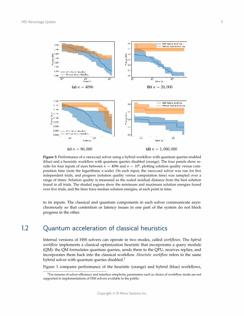
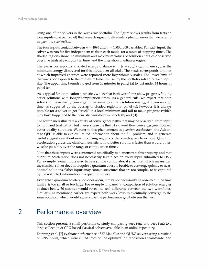
Figure 3: Performance of a version2 solver using a hybrid workflow with quantum queries enabled(blue) and a heuristic workflow with quantum queries disabled (orange). The four panels show re-sults for four inputs of sizes between n = 4096 and n = 106, plotting solution quality versus com-putation time (note the logarithmic x-scale). On each input, the version2 solver was run for fiveindependent trials, and progress (solution quality versus computation time) was sampled over arange of times. Solution quality is measured as the scaled residual distance from the best solutionfound in all trials. The shaded regions show the minimum and maximum solution energies foundover five trials, and the lines trace median solution energies, at each point in time.

to its inputs. The classical and quantum components in each solver communicate asyn-chronously so that contention or latency issues in one part of the system do not blockprogress in the other.

1.2 Quantum acceleration of classical heuristics

Internal versions of HSS solvers can operate in two modes, called workflows. The hybridworkflow implements a classical optimization heuristic that incorporates a query module(QM): the QM formulates quantum queries, sends them to the QPU, receives replies, andincorporates them back into the classical workflow. Heuristic workflow refers to the samehybrid solver with quantum queries disabled.3

Figure 3 compares performance of the heuristic (orange) and hybrid (blue) workflows,

3For reasons of solver efficiency and interface simplicity, parameters such as choice of workflow mode are notsupported in implementations of HSS solvers available to the public.



using one of the solvers in the version2 portfolio. The figure shows results from tests onfour inputs (one per panel) that were designed to illustrate a phenomenon that we refer toas quantum acceleration.

The four inputs contain between n = 4096 and n = 1, 000, 000 variables. For each input, thesolver was run for five independent trials in each mode, for a range of stopping times. Theshaded regions show the minimum and maximum values of solution energies e observedover five trials at each point in time, and the lines show median energies.

The y-axis corresponds to scaled energy distance δ = (e − emin)/emin, where emin is theminimum energy discovered for this input, over all trials. The x-axis corresponds to timesat which improved energies were reported (note logarithmic x-scale). The lower limit ofthe x-axis corresponds to the minimum time limit set by the portfolio solver for each inputsize. The upper time bounds ranged from 20 minutes in panel (a) to just under 14 hours inpanel (c).

As is typical for opimization heuristics, we see that both workflows show progress, findingbetter solutions with longer computation times. As a general rule, we expect that bothsolvers will eventually converge to the same (optimal) solution energy, if given enoughtime, as suggested by the overlap of shaded regions in panel (c); however it is alwayspossible for a solver to get “stuck” in a local minimum and fail to make progress (whichmay have happened to the heuristic workflow in panels (b) and (d).

The four panels illustrate a variety of convergence paths that may be observed, from inputto input and trial to trial, but in every case the the hybrid workflow converges faster towardbetter-quality solutions. We refer to this phenomenon as quantum acceleration: the Advan-tage QPU is able to exploit limited information about the full problem, and to generateuseful suggestions about new promising regions of the search space to explore. Quantumacceleration guides the classical heuristic to find better solutions faster than would other-wise be possible, over the range of computation times.

Note that these inputs were constructed specifically to demonstrate this property, and thatquantum acceleration does not necessarily take place on every input submitted to HSS.For example, some inputs may have a simple combinatorial structure, which means thatthe classical solver does not require a quantum boost to be able to converge quickly to near-optimal solutions. Other inputs may contain structures that are too complex to be capturedby the restricted information in a quantum query.

Even when quantum acceleration does occur, it may not necessarily be observed if the timelimit T is too small or too large. For example, in panel (a) comparison of solution energiesat times below 30 seconds would reveal no real difference between the two workflows.Similarly, as mentioned earlier, we expect both workflows to eventually converge to thesame solution, which would again close the performance gap between the two.

2 Performance overviewThis section presents a small performance study comparing version1 and version2 to alarge collection of CPU-based classical solvers available in an online repository.

Dunning et al. [7] evaluate performance of 37 Max Cut and QUBO solvers using a testbedof 3296 inputs, which were culled from online optimization repositories worldwide, and



Figure 4: Performance of HSS version1 (blue) and version2 (orange) solvers on MQLib inputs. Ineach pair, the blue bars show the proportion of wins (darker) and ties (lighter) achieved by version1

in comparison to MQLib. The orange bars show proportion of wins (darker) and (lighter) achievedby version2 in comparison to MQLib. The first six pairs of bars describe performance on 45 originalMQLib inputs, divided into groups according to graph density (sparse, medium, dense) and size(small, medium large). The next bar marked hybrids shows a head-to-head comparison of version1(blue) and version 2 (orange), with ties marked in teal. The rightmost bar x-large compares perfor-mance of version2 against MQLib solvers on 20 very large inputs that are too big for version1.

translated to Max Cut and QUBO form for this repository. The solvers, inputs, and dataanalysis tools from this extensive project are available from the MQLib repository (see [7]).

As mentioned in Section 1.2, solver-to-solver differences in solution quality tend to disap-pear when heuristic solvers are allowed long runtimes, because many will eventually con-verge to the same (optimal) solution energy. Similarly, performance differences are hardto detect when solvers are allowed very short runtimes, because initial solutions tend tobe more-or-less random. Thus distinctions in solver performance with respect to solutionquality can only be observed when time limits used in the experiment are somewere be-tween these two extremes.

For this reason, for each input Q the authors provide a recommended time limit TQ, shortenough that only a small number of solvers were able to match the best solution cost CQfound. Running multiple tests for the recommended time limit makes it possible to observesystematic differences in solver performance.

In their tests, all solvers ran for five independent trials using recommended time limits.Thus we may consider CQ to be the best result that would be observed by a hypotheticalparallel portfolio running five independent copies of each solver, totaling 185 solvers. Herewe refer to CQ as the reference cost, or reference energy.

Our tests use two subsets of MQLib inputs that are selected from among the “hardest” inMQLib. That is, all have a maximum recommended time limit of TQ = 20 minutes, andin each case the reference cost was found by only one or two MQLIb solvers: that is, theremaining solvers found strictly worse solutions. The inputs were selected at random inbatches to cover a range of sizes and densities: see Appendix A.2 for details.

To match the MQLib test design, for each input we ran five independent trials of a singlesolver from version1 and a single solver from version2, for 20 minutes per trial. In termsof computational resource usage, the 37 × 5 MQLib tests required 62 CPU-hours of totalwork per input, or 20 minutes using 185-fold parallelization. Five trials of a single HSS



solver required 1.7 (CPU/GPU) hours of classical work per input (running in tandem withthe QPU), or 20 minutes using 5-fold parallelization.

Our first experiment compares performance of the version1 and version2 solvers againstthe best of 37 MQLib solvers, using a set of 45 inputs from the MQLib repository (the“standard set”) that are small enough to fit on both solvers. The second experiment looksat performance of the version2 solver on an additional 20 inputs (the “x-large set”) thatare too large for version1 and among the largest available in MQLib. Details about inputproperties and our selection procedure may be found in Appendix A.2.

For each input Q we record the best solution energy obtained from five independent trialsof each hybrid solver, and compare it to the MQLib reference cost CQ (the best found in alltrials of all 37 solvers). For each input there are three possible outcomes: the best solutionenergy found by the hybrid solver in five trials is lower than (win), equal to (tie), or higherthan (lose) the reference cost.4

Figure 4 presents the tallys for the two HSS solvers.

The leftmost group of bars shows performance of version1 (blue) and version2 (orange)solvers versus MQLib solvers, using our standard set of 45 inputs. These inputs fall intothree groups of 15 according to graph density (dense, medium, sparse); the same inputs fallinto three groups of 15 according to graph size (small, medium, large), totaling 9 groups of5 inputs each.

The next bar, labeled “hybrids,” shows results of a head-to-head comparison of version1and version2 on the 45 standard inputs, with ties marked in teal. The rightmost bar la-belled “x-large” shows a comparison of version2 to the MQLib solvers on the 20 extra-large inputs (no ties).

Hybrid solvers versus MQLib on standard inputs. The first group of six pairs shows testresults for “standard” inputs organized by density (sparse, medium, dense) and by size(small, medium, large). The blue bars show performance of the version1 solver using the2000Q quantum processor, versus 37 MQLib solvers, and orange bars show performanceof the version2 solver using Advantage system (orange), again versus the MQLib 37. Thelength of each bar shows the proportion of tests that resulted in wins (darker blue or or-ange) or ties (lighter blue or orange) for the HSS solvers. The grey sections of each bar showthe proportion of wins for MQLib solvers.

In the first three cases (sparse, medium, dense) we see that the version2 solver signifi-cantly outperforms the version1 solver on sparse inputs, improving from wins-or-ties on40 percent of tests (6 of 15) up to 87 percent of tests (12 of 15). This improvement reflectsa combinaton of software enhancements and the move from the D-Wave 2000Q to Advan-tage as a back-end query server. On medium and dense inputs, the two hybrid solversshow about the same performance.

Considering the next three cases (small, medium, large) we observe that the version2

solver shows good improvement over version1 on all three size categories, with greaterperformance gap seen on small and medium-sized inputs.

4A look at the data suggests that some wins and losses are by very small margins, and may in fact be mis-recorded ties. That is, it is possible that the same solution gives rise to slightly different costs when they arecalculated in different computing environments, due to numerical precision issues for the enormous input sizesbeing tested. However, there is no way to verify this hypothesis without access to the original solutions andcalculations used in MQLib.



Over all 45 inputs in this test, the version1 solver has 27 wins and 3 ties versus the bestof 37 MQLib solvers, totalling 67 percent, while the version2 solver has 34 wins and 4 tiesversus MQLib solvers, totalling 84 percent.

version1 versus version2 on standard inputs. The next column labeled “hybrids” showsresults of a head-to-head comparison of the two hybrid solvers on the set of 45 standardinputs. Here, version2 solver found better solutions in 35 cases (78 percent), and the twosolvers tied in 5 cases (11 percent). We attribute the superior performance of version2 toa combination of coding and algorithmic improvements to the hybrid software — partic-ularly targeting performance on sparse inputs — and to the upgrade from the 2000-qubit2000Q QPU to the 5000-qubit Advantage QPU as the back-end quantum query server.

version2 vs MQLib solvers on extra-large inputs. The rightmost bar of Figure 4 showsresults for the 20 extra-large MQLib inputs, of sizes between N > 1000 and N = 53, 130(the largest available in MQLib). On these inputs, in five trials the version2 solver foundbetter solutions than the best of 37 MQLib solvers (each run for five trials, totaling 185trials), on exactly half of the inputs.

Because none of the extra-large inputs in MQLib meet our selection criteria for mediumand dense inputs, all 20 inputs in the test set are categorized as sparse. Within that context,we observe that version2 tends to perform relatively better on the less-sparse problems inthis test set. See Appendix 2.1 for details about the inputs used in these tests.

More extensive evaluation of our hybrid solvers, on a variety of inputs in the full rangeof sizes that can be accomodated by version2, is of course an interesting question futureresearch. Progress on this front has been somewhat hampered by unavailability of suitableclassical competition that can also handle the larger input sizes; however we look forwardto removal of this temporary obstacle in the next several months.

3 SummaryThis report describes general features and properties of the upgraded D-Wave hybridsolver service avalailable as of September 2020, and presents a preliminary look at hybridsolver performance. A comparison of an earler version1 solver to an upgraded version2

solver in the HSS portfolio shows that version2 significantly outperforms version1. Bothsolvers outperform a collection of 37 classical solvers available in a public repository, whentested on a wide variety of inputs that have structures that are relevent to applicationspractice.

We look forward to future work to expand this preliminary study with more tests compar-ing performance of solvers in the HSS portfolio against state-of-the-art classical solvers, ona greater variety of inputs of relevance to applications practice.



References1 D-Wave Applications, (web page and search tool), available at http://dwavesys.com/applications, accessed September 2020.

2 D-Wave Hybrid, http://github.com/dwavesystems/dwave-hybrid, accessed February 2020.

3 D-Wave Ocean, http://ocean.dwavesys.com, accessed February 2020.

4 D-Wave Leap, http://cloud.dwavesys.com/leap, accessed February 2020.

5 C. McGeoch and P. Farre, The D-Wave Advantage System: An Overview, https://dwavesys.com/resources/publications (D-WaveTechnical Report 14-1049A-A, 2020).

6 C. McGeoch and P. Farre, Discrete Quadratic Model Solver: An Overview, https://dwavesys.com/resources/publications (D-WaveTechnical Report (to appear), 2020).

7 Dunning et al., “What works best when? A systematic evaluation of heuristics for Max-Cut and QUBO,” INFORMS Journal on Com-puting 30, also visit http://github.com/MQLib (2018).

8 D-Wave Documentation: Hybrid Solvers, https://docs.ocean.dwavesys.com/en/stable/overview/hybrid.html, accessed August2020.


http://dwavesys.com/applications

http://github.com/dwavesystems/dwave-hybrid

http://ocean.dwavesys.com

http://cloud.dwavesys.com/leap

https://dwavesys.com/resources/publications

https://dwavesys.com/resources/publications

http://github.com/MQLib

https://docs.ocean.dwavesys.com/en/stable/overview/hybrid.html


A Details of the experimentsThis appendix presents details of our test protocols as well as the inputs and solvers se-lected for study.

A.1 Measurement and metrics

The hybrid DW solvers evaluated here have code components that run on three types ofplatforms: CPU, GPU, and QPU. In everyday use, for some given input, a front-end portfo-lio solver selects some number of solvers (programs implementing specific heuristics) andsome number of CPU and GPU platforms to be used in the computation.

At present, HSS contains two portfolio solvers, one from the original launch and an up-graded version that reads larger inputs and incorporates an Advantage QPU instead ofthe 2000Q QPU. In our tests, both portfolios are set to choose one hybrid solver for allinputs, which we call version1 and version2. Both versions run in asynchronously in adistributed computing framework, sending quantum queries to their respective quantumprocessors and incorporating QPU responses when they arrive.

Naturally this arrangement creates considerable challenges in obtaining accurate and re-peatable runtime measurements. Our policies for measuring and reporting runtimes wereas follows:

• The CPU and GPU code ran in a p3.2xlarge AWS instance containing an NVIDIATesla V100 platform with 16GB memory, 60Gb of RAM and eight virtual cores; and anIntel Xeon(R) E5-2686 v4 (Broadwell) platform. CPU time measurements were takenwith hyperthreading turned on.

• Programming languages used in this system include python, cython, C++, and C++with the CUDA toolkit. C++ code was always compiled with the -Ofast or -O3 opti-mization flags; the CUDA compiler has optimization turned on by default.

• Quantum queries were sent to a D-Wave 2000Q low-noise system (version1 and toa D-Wave Advantage system version2 located at D-Wave headquarters in Burnaby,BC. Quantum algorithm parameters were set to default values throughout: 20µs an-neal time and 1000 reads per input.

• Elapsed computation time for the portfolio solver is specified by the user as a timelimit T. The global runtime clock starts and finishes on the same platform, in a singlethread that forks the processes needed to invoke solvers on other platforms. The childprocesses are responsible for monitoring their own progress and sending solutions tothe parent process before the time limit T is reached.

• Since individual solvers work in parallel and communicate asynchronously with theQPU, total computation time does not equal the sum of component times. Note thatthis design ensures that computational progress is not stalled by issues such as net-work latency or contention for the QPU, which are impossible to control or predict.



A.2 MQLib

The MQLib repository [7] contains 3296 inputs for Max Cut or QUBO problems and acollection of 10 Max Cut and 27 QUBO heuristic solvers. The solvers are implemented inC++ and run on standard CPU cores. It also contains an extensive collection of supporttools for, e.g., translating inputs between problem formulations, running tests, analyzingresults, and selecting the best solvers for any given input.

We did not carry out independent tests using these solvers, but instead refered to publishedperformance data available in the MQLib repository. In particular, the /data/ directorycontains a recommended run time limit T for each input, and a reference cost obtained byrunning all 37 solvers the time limit T, over five independent trials each. Our tests use thesame time limit and record solution costs obtained in five independent trials of the DWhybrid solver.

Solvers MQLib runtime measurements on 37 solvers were performed in 2018 using AWScores, as follows [7]:

We performed heuristic evaluation using 60 m3.medium Ubuntu machines fromthe Amazon Elastic Compute Cloud (EC3), which have Intel Xeon E5-2670 pro-cessors and 4 GiB of memory; code was compiled with the g++ compiler usingthe -O3 optimization flag.

The authors report that their full evaluation (37 solvers and 3296 inputs) required 2 CPU-years of processing power, 12.4 days of computation (over 60 machines), and cost $1196.00in AWS compute time.

Inputs For the “standard” test set described in Section 2, we selected 45 instances fromthe MQLib repository using the following procedure.

• The MQLib designers noted that results tend to be similar or identical when allsolvers are given either too little or too much time to work on a given instance. Thus,to each instance they assign a suggested runtime T that can be used to distinguishperformance among solvers.

Our selection protocol considered only “hard” instances with a maximum recom-mended runtime of T = 20 minutes, and instances for which at most two of the 37solvers found the best reported solution. On 42 of the 45 inputs exactly one solverfound that solution; on the remaining three inputs, two solvers tied.

• Inputs that are unconnected, contain fewer than n = 1000 variables, or more thann = 10, 000 variables, were not selected for the standard set.

• The remaining input pool was partitioned into groups according to size [small (1000 ≤n ≤ 2500), medium (2500 < n ≤ 5000) and large (5000 < n ≤ 10000)] and edge den-sity [sparse (d ≤ 0.1M), medium (0.1M < d ≤ 0.5M), and dense (d > 0.5M)]. Here dis the mean edge density of the instance and M is the number of edges in a completegraph with n nodes. This yields nine input groups: for each group we select 5 inputsuniformly at random after filtering as described above.



• Inputs stored in Max Cut form in MQLib were translated to an equivalent QUBOform for testing on our system.

For the “extra-large” input set we filtered the MQLib input set as described above. We se-lected 20 inputs uniformly at random from the resulting filtered set, with sizes n > 10, 000.This selection process included the largest input in MQLib, which contains n = 53, 130nodes.

The extra-large MQLib inputs are extremely sparse, and fail to meet our criteria for mediumand dense inputs. The selected inputs in this group have sizes in range 24, 052 ≤ n ≤53, 130, and densities in range .000095M ≤ d ≤ .0031M

Both sets of inputs, translated from MQLib (Max Cut) format to D-Wave DIMOD (QUBO)format, are available at the D-Wave github site github.com/dwavesystems/hss-overview-benchmarks.


d-wave hybrid solver service + advantage: technology update

Documents