d spinning top: discretization visualization · theorem 1.1 (kirchhoffs kinetic analogy). the paths...
TRANSCRIPT

DYNAMICS OF THE SPINNING TOP: DISCRETIZATIONAND INTERACTIVE V ISUALIZATION
Diploma Thesis
byRené Bodack
Technische Universität BerlinInstitut für Mathematik
Prof. A. I. Bobenko
Berlin, August 18, 2008

Die selbstständige und eigenhändige Anfertigungversichere ich an Eides statt.
Berlin, 18. August 2008

Contents
1 Introduction 1
2 The Spinning Top 52.1 Definition . . . . . . . . . . . . . . . . . . . . . . . . . . . . . . . . . . . . . . . . . . 52.2 Motion, vector of angular velocity, vector of angular momentum . . . . . . . . . . . . . 52.3 Moments of inertia, inertia tensor, body frame. . . . . . . . . . . . . . . . . . . . . . . 7
2.3.1 General. . . . . . . . . . . . . . . . . . . . . . . . . . . . . . . . . . . . . . . 72.3.2 Application to a quader, notations. . . . . . . . . . . . . . . . . . . . . . . . . 10
2.4 The Lagrange top. . . . . . . . . . . . . . . . . . . . . . . . . . . . . . . . . . . . . . 16
3 Dynamics 193.1 Variational principals. . . . . . . . . . . . . . . . . . . . . . . . . . . . . . . . . . . . 193.2 Rotation inR3, su(2) andSU(2) . . . . . . . . . . . . . . . . . . . . . . . . . . . . . . 21
3.2.1 The vector spacesu(2) . . . . . . . . . . . . . . . . . . . . . . . . . . . . . . . 213.2.2 The matrix groupSU(2) . . . . . . . . . . . . . . . . . . . . . . . . . . . . . . 22
3.3 Energy of the spinning top. . . . . . . . . . . . . . . . . . . . . . . . . . . . . . . . . 253.4 Equation of motion of the spinning top in the rest frame. . . . . . . . . . . . . . . . . . 253.5 Elastic curves and spinning tops. . . . . . . . . . . . . . . . . . . . . . . . . . . . . . 30
4 Discretizations 334.1 Numerical discretizations. . . . . . . . . . . . . . . . . . . . . . . . . . . . . . . . . . 33
4.1.1 Extrap - The Gragg-Burlisch-Stoer extrapolation algorithm . . . . . . . . . . . . 334.2 Integrable discretization by A. I. Bobenko and Yu. B. Suris . . . . . . . . . . . . . . . . 34
4.2.1 Calculation in a scaled coordinate system. . . . . . . . . . . . . . . . . . . . . 344.2.2 Notations. . . . . . . . . . . . . . . . . . . . . . . . . . . . . . . . . . . . . . 364.2.3 Results . . . . . . . . . . . . . . . . . . . . . . . . . . . . . . . . . . . . . . . 36
5 Calculation and the Top Visualization 395.1 JReality . . . . . . . . . . . . . . . . . . . . . . . . . . . . . . . . . . . . . . . . . . . 395.2 Move, look around, open panels. . . . . . . . . . . . . . . . . . . . . . . . . . . . . . 395.3 Change jReality configuration. . . . . . . . . . . . . . . . . . . . . . . . . . . . . . . 39
5.3.1 2D view of the scene. . . . . . . . . . . . . . . . . . . . . . . . . . . . . . . . 405.4 Loaded content: A Lagrange top example. . . . . . . . . . . . . . . . . . . . . . . . . 405.5 A first test run, the buttonsStart/StopandStep. . . . . . . . . . . . . . . . . . . . . . . 405.6 Change top and motion settings. . . . . . . . . . . . . . . . . . . . . . . . . . . . . . . 40
5.6.1 Rotate quader. . . . . . . . . . . . . . . . . . . . . . . . . . . . . . . . . . . . 405.6.2 Change size. . . . . . . . . . . . . . . . . . . . . . . . . . . . . . . . . . . . . 405.6.3 Change fixed point. . . . . . . . . . . . . . . . . . . . . . . . . . . . . . . . . 41
i
ii CONTENTS
5.6.4 Edit vector of kinetic momentum. . . . . . . . . . . . . . . . . . . . . . . . . 425.6.5 Epsilon, speed and gravity. . . . . . . . . . . . . . . . . . . . . . . . . . . . . 425.6.6 The Kowalewski and Goryachev-Chaplygin cases. . . . . . . . . . . . . . . . . 43
5.7 Elastic rods and the apex trace. . . . . . . . . . . . . . . . . . . . . . . . . . . . . . . 445.7.1 Kirchhoffs analogy visualized. . . . . . . . . . . . . . . . . . . . . . . . . . . 445.7.2 Analogy of tops and anisotropic elastic rods visualized . . . . . . . . . . . . . . 465.7.3 The apex trace visualized. . . . . . . . . . . . . . . . . . . . . . . . . . . . . . 46
5.8 The Lagrange top mode. . . . . . . . . . . . . . . . . . . . . . . . . . . . . . . . . . . 485.8.1 Same motion calculated with Bobenko-Suris discretization . . . . . . . . . . . . 485.8.2 The stoptime. . . . . . . . . . . . . . . . . . . . . . . . . . . . . . . . . . . . 485.8.3 Quader distance. . . . . . . . . . . . . . . . . . . . . . . . . . . . . . . . . . . 495.8.4 Epsilon2 . . . . . . . . . . . . . . . . . . . . . . . . . . . . . . . . . . . . . . 495.8.5 The timer. . . . . . . . . . . . . . . . . . . . . . . . . . . . . . . . . . . . . . 50
5.9 Comparing discretizations, Eps2Tab and Diagrams tab. . . . . . . . . . . . . . . . . . 505.9.1 Visual comparison. . . . . . . . . . . . . . . . . . . . . . . . . . . . . . . . . 505.9.2 Error in the body frame. . . . . . . . . . . . . . . . . . . . . . . . . . . . . . . 505.9.3 Integrals of motion. . . . . . . . . . . . . . . . . . . . . . . . . . . . . . . . . 51
6 Results 536.1 Comparison of theBobenko-Suris discretizationto theExtrapmethod . . . . . . . . . . 53
6.1.1 Settings. . . . . . . . . . . . . . . . . . . . . . . . . . . . . . . . . . . . . . . 536.1.2 Visual results. . . . . . . . . . . . . . . . . . . . . . . . . . . . . . . . . . . . 556.1.3 Error in the body frame. . . . . . . . . . . . . . . . . . . . . . . . . . . . . . . 556.1.4 Error in the integrals of motion. . . . . . . . . . . . . . . . . . . . . . . . . . . 586.1.5 Further Observations. . . . . . . . . . . . . . . . . . . . . . . . . . . . . . . . 61
6.2 Comparison of theBobenko-Suris discretizationto Extrapcomprising execution time. . 616.2.1 Settings. . . . . . . . . . . . . . . . . . . . . . . . . . . . . . . . . . . . . . . 636.2.2 Visual results. . . . . . . . . . . . . . . . . . . . . . . . . . . . . . . . . . . . 646.2.3 Error in the body frame. . . . . . . . . . . . . . . . . . . . . . . . . . . . . . . 646.2.4 Error in the energy. . . . . . . . . . . . . . . . . . . . . . . . . . . . . . . . . 64
6.3 Comparison of theBobenko-Suris discretizationto theRunge-Kuttamethod . . . . . . . 696.4 Conclusions. . . . . . . . . . . . . . . . . . . . . . . . . . . . . . . . . . . . . . . . . 696.5 Prospects . . . . . . . . . . . . . . . . . . . . . . . . . . . . . . . . . . . . . . . . . . 70
Appendices 71
A Abstract in german - Zusammenfassung auf Deutsch 71

Chapter 1
Introduction
The spinning top, a rigid body moving around a fixed point in a homogeneous gravity field, is a famoustopic in classical mechanics. Its non-linear equations of motion are the well known Kirchhoff equations,whose discretization and hence actual calculation is topicof the present work. In order to achieve qualitypath discretizations it is advisable to use all present knowledge of the mechanical system, e. g. the factthat they preserve their energy, and hence have a so called integral of motion. Yet the Kirchhoff equationshave only two such integrals, so they are not integrable and there is no integrable discretizations as well.There are, though, integrable special cases of spinning topmotion. One of them is the Lagrange top, arotationally symmetric body with the fixed point on the symmetry axis. Then the third component of thevector of angular momentum in the body frame (a frame firmly attached to the body and the origin atthe fixed point) is a third integral of motion, additional to the energy and third component of the angularmomentum in the rest frame (a frame constant in time, so that the gravity is parallel to the third axis),which are always constant. This assures its complete integrability. But only recently Prof. A. I. Bobenkoand Prof. Yu. B. Suris found an integrable discretization for the Lagrange tops path. In [BS00], they usedthe following
Theorem 1.1(Kirchhoffs kinetic analogy). The paths of Lagrange top body frames are in a one to onecorrespondence to the frames of elastic curves.
to derive an integrability preserving discretization, which will be called theBobenko-Suris discretiza-tion from now on. Elastic curves are thereby curves that minimizetheir bending energy for fixed length,boundary points and velocity vectors at the boundary.
Comparison of theBobenko-Suris discretization to numerical ones In the present work now a qualita-tive assessment of this discretization is done. This is achieved with an actual calculation and visualizationin aJavaTM application calledTop Visualization. To have a comparison to existing discretizations, the topspaths are calculated in essentially three different ways for identical initial data: once with a very smalldiscretization step length parameterε to have a result close to the "real", the continuous one; second witha known numerical discretization with a biggerε, i. e. to have a really discrete motion; and third with theintegrable discretization with again a bigε.
As result, two things turn out clearly. First theBobenko-Suris discretizationhas a flaw. Denotingmthe vector of angular momentum,a the vector pointing to the center of mass andg the gravity vector, allin the rest frame, theBobenko-Surisdiscretization doesnot preserve the energy of the Lagrange top
H =1
2〈m, m〉 + 〈a, p〉 .
1

2 CHAPTER 1. INTRODUCTION
Figure 1.1: Errors in the energy for the numerical and theBobenko-Suris discretization. In the beginningthe numerical error is small, but it propagates somewhat quadratic so it surpasses the oscillating error inthe integrable case eventually.
Instead it preserves the term
Hε =1
2〈m, m〉 + 〈a, p〉 +
ε
2〈a × m, p〉 .
The additional term causes a quite high deviation from the real energy, which in turn results in an errorin the tops body frame. So the calculated path is a different one from the continuous, which showsitself already after short time periods. Nontheless, the second observation is that, though the numericaldiscretization is always better in the beginning, eventually its errors will exceed the ones of the integrablediscretization. In figure1.1 it can be seen that the numerical error propagation is somewhat quadratic,whereas the error in theBobenko-Suris discretizationoscillates.
Visualizations Once the program was written to find these results, it lent itself to enhance its function-ality to other interesting visualizations. There are now, for instance, two more integrable cases of rigidbody motion visualized, namely theKowalewskiand theGoryachev-Chaplygintops.1
In order to visualize them, the numerical calculation of thetop motion was implemented for generalspinning tops. For that it proved useful to find a form of the Kirchhoff equations in the rest frame, whichreads
ω′ = A−1(Aω × ω + M· p × a) where
A = IN · NN t + IB · BBt + IT · TT t.
Therebyω is the vector of angular velocity,M the total mass,(N, B, T ) the body frame andIN , IB ,IT the principal moments of inertia of the body. The gravity vector is then the (constant) third rest framevector and the path of the body frame can be reproduced fromω.
Furthermore there is a visualization of Kirchhoffs kineticanalogy1.1and also of its generalization toelastic rods, i. e. when including a twist energy as penalityfor torsion of the rod. Elastic curves then areisotropic elastic rods, which have a symmetric cross section (e. g. round or square). The generalizationis then that elastic rods in general correspond to spinning tops with the fixed point on one of its principalaxes. Now, there are Kowalewski and Goryachev-Chaplygin tops with that property, so there exists acorresponding elastic rod. These corresponding objects are visualized together in theTop Visualization
1The last integrable case is the Euler top, having its fixed point at the center of mass. But this one is already well known andnotvery interesting to visualize.

3
(a) A Goryachev-Chaplygin top with its corresponding(anisotropic) elastic rod.
(b) A Lagrange top with its precession and nutation visu-alized in the so calledapex trace.
Figure 1.2: Example visualizations.
program, and also the isotropic elastic rods correspondingto Lagrange tops can be studied. For anexample of a Goryachev-Chaplygin top with its corresponding elastic rod see figure1.2(a).
Studying spinning top motions is not limited to special cases either in theTop Visualizationprogram.One starts with a certain quader, but can edit it to arbitraryquader with arbitrary fixed points; and sincethe motion of spinning tops is determined by its fixed point and its principal moment of inertia, the motionof the body frame of every spinning top can be seen.
Finally there is a visualization of the typical 2-periodic behaviour of the symmetry axis of Lagrangetops, the so called precession and nutation. Therefore the point of intersection of the symmetry axis witha sphere around the bodys fixed point is drawn and connected atevery motion step. This so calledapextracecan be seen at an example in figure1.2(b).
The thesis is organized as follows:In chapter2 the basics about spinning tops in general and the Lagrange top in special are recalled.
In examples these are applied to quader, which are the special case of spinning tops used in theTopVisualizationprogram.
Chapter3 is devoted to the continuous dynamics of spinning tops. There basic variational principlesand the matrix groupssu(2) andSU(2) are recalled, with whose help the formulation of Kirchhoffsequations in the rest frame is then derived. Further the derivation of Kirchhoffs kinetic analogy and itsgeneralization is given at the end of this chapter.
Chapter4 is devoted to the different discretizations of the paths of spinning tops. First the basicfacts on the numerical discretization used in theTop Visualizationprogram are given, then the integrablediscretization found by Prof. A. I. Bobenko and Prof. Yu. B. Suris is presented. For its derivation see theoriginal paper [BS00].
The complete description, functionality and features of the Top Visualization program aregiven in chapter5. The program can be found on the CD attached to the back cover,underhttp://www.math.tu-berlin.de/˜bodack or as webstart application underhttp://www.math.tu-berlin.de/geometrie/ps/software.shtml and used to compare the discretizationsoneself.
The results of an exemplary comparison are given in chapter6. Further there are the results of twoother, non-repeatable experiments given in chapter6 which give additional insight into the properties oftheBobenko-Suris discretization.

4 CHAPTER 1. INTRODUCTION

Chapter 2
The Spinning Top
2.1 Definition
Definition. A rigid body is a set of points in euclidean space which move in time and preserve theirdistance, i. e.
‖x(t) − y(t)‖ = const ∀t (2.1)
wheret is the time andx andy two points of the body moving witht. Or more precisely,x, y : T → R3,t 7→ x(t), t 7→ y(t), t ∈ T are continuous functions.
Definition. A fixed pointis a point in euclidean space which stays constant in time.
Definition. A spinning topis a rigid body in a homogeneous1 gravitational field that moves around afixed point, i. e.
‖x(t) − O‖ = const ∀t, x, y (2.2)
whereO is the fixed point andx a point of the body.
Example.The spinning top used in theTop Visualizationprogram desribed in chapter5 is a homogeneousquader, the fixed point is at the origin and (in most of the examined cases) at the center of one of the quaderfaces. See figure2.1.
2.2 Motion, vector of angular velocity, vector of angular momen-tum
Definition. Thevector of angular velocityat timet of a rigid body rotating around the origin is the vectorω(t) ∈ R3 that satisfies
x(t) = ω(t) × x(t) (2.3)
for all points of the body.
Remark.The general case of motion of a rigid body can be described by adisplacement of the center ofmass of the body plus a rotation around it.
The spinning top motion is limited to a rotation around the fixed point and is therefore determined bythree independent variables. Knowledge of the instantaneous rotation axis and the rotation speed therefore
1constant
5

6 CHAPTER 2. THE SPINNING TOP
Figure 2.1: Quader with fixed point at the center of one of its faces.
Figure 2.2: Quader with its vector of angular velocity.
completely suffices. It can be unified in thevector of angular velocity, which points in the direction ofthe rotation axis and has the length of the rotation speed. Itis usually denoted withω. The direction ofthe vector can be determined by theright hand rule2.
Example.The vector of angular velocity in theTop Visualizationprogram is blue. See figure2.2.
Definition. Thevector of angular momentumm(t) of a pointx(t) with massM is defined by
m(t) = x(t) ×Mx(t),
i. e. the cross product of the point with itslinear momentum.For a body within the areaV with mass density functionρ(q) the vector of angular momentum is
m(t) :=
∫
V
q(t) × ρ(q) q(t) dq.
2Point your right thumb up, curl the other fingers, they show the direction of the rotation.

2.3. MOMENTS OF INERTIA, INERTIA TENSOR, BODY FRAME 7
Figure 2.3: Quader with its vector of angular velocity (blue) and vector of angular momentum (green).
Example.The vector of angular momentum in theTop Visualizationprogram is green. See figure2.3.
2.3 Moments of inertia, inertia tensor, body frame
2.3.1 General
Definition. Themoment of inertiaof a body wrt an axisl is
Il :=
∫
V
ρ(q) r2l (q) dq (2.4)
whereρ is the density function of the body,V ⊂ R3 a region containing the body andrl(q) the distance
of q to thel axis.3
Remark.Physically the moment of inertia is for a rotational acceleration what the mass is for a rectilinearone. It is a measure for the resistance against acceleratingthe body around the axisl.
There is a connection between thevector of angular velocity, thevector of angular momentumandthemoments of inertiaof a body, the so calledinertia tensor. It will prove useful to unite allmoments ofinertia of a body rotating around a fixed point and yield thebody frameof the body, with whose help thecalculation of the body motion will be much simplified.
Definition. The inertia tensorof a rigid body is that linear mappingJ which maps the body’svector ofangular velocityto itsvector of angular momentum, i. e.
m = Jω. (2.5)
Remark(Existence and calculation). If the body is contained in the regionV and has density functionρ,
3For a body containing only a finite number of points the integral changes to a sum.

8 CHAPTER 2. THE SPINNING TOP
then in shortened notation:
m =
∫
V
q × ρ(q) q dq
def=
∫
V
ρ(q) · q × (ω × q) dq
(2.6)=
∫
V
ρ(q) ·(ω 〈q, q〉 − q 〈q, ω〉
)dq
(2.7)=
∫
V
ρ(q) ·(〈q, q〉E(3) − q · qt
)dq · ω
TherebyE(3) denotes the unit3 × 3 matrix. Further thebac-cabrule
a × (b × c) = b 〈a, c〉 − c 〈a, b〉 (2.6)
and〈a, b〉 a = (a · at) · b (2.7)
were used. Hence
J =
∫
V
ρ(q) ·(〈q, q〉E(3) − q · qt
)dq.
The latter integral depends on the origin of the chosen coordinate system (the fixed point), soJ does too.Now for a given body the vector of angular momentum can be calculated from the vector of angular
velocity and vice versa. The connection between the inertiatensor and the moments of inertia clarifiesthe following
Lemma 2.1. Let J be the inertia tensor of a body wrt the fixed point (the origin)and l an axis throughthe origin, then the moment of inertia of the body wrtl is
Il = ~lt · J ·~l =⟨~l, J~l
⟩(2.8)
where~l is a unit vector spanningl.
Proof.
⟨~l, J~l
⟩=
⟨~l,
∫
V
ρ(q) ·(⟨
q, q⟩E(3) − q · qt
)dq ·~l
⟩
=
∫
V
ρ(q)⟨~l,(⟨
q, q⟩E(3) − q · qt
)·~l⟩
dq
=
∫
V
ρ(q)(⟨
q, q⟩⟨
~l,~l⟩−~lt · q · qt ·~l
)dq
=
∫
V
ρ(q)(⟨
q, q⟩−⟨~l, q⟩⟨
q,~l⟩)
dq
Sincerl, the distance of the pointq to the axisl, satisfies
rl2(q) =
⟨q, q⟩−⟨q,~l⟩2
(2.9)

2.3. MOMENTS OF INERTIA, INERTIA TENSOR, BODY FRAME 9
(Pythagorean theorem) we get
⟨~l, J~l
⟩=
∫
V
ρ(q) · rl2(q) dq = Il
Another interesting property of the inertia tensor gives the following
Lemma 2.2. The inertia tensorJ is symmetric.
Proof. It is to show that for arbitrary vectorsa andb it holds
〈a, Jb〉 = 〈Ja, b〉 .
Now
〈a, Jb〉 =
⟨a,
∫
V
ρ(q)(〈q, q〉E(3) − q · qt
)dq · b
⟩
=
⟨a,
∫
V
ρ(q)(〈q, q〉 b − q · qt · b
)dq
⟩
=
∫
V
ρ(q)⟨a,(〈q, q〉 b − q 〈q, b〉
)⟩dq
(2.6)=
∫
V
ρ(q) 〈a, q × (b × q)〉 dq
=
∫
V
ρ(q) 〈b × q, a × q〉 dq, (2.10)
where the last step is the circular symmetry of the triple scalar product (the determinant).The fact that the last expression is symmetric wrta andb completes the proof.
As a first conclusion, one can calculate the kinetic energy ofthe body with the help of the inertiatensor.
Corollary 2.3. Let a rigid body be fixed at the origin,J be its inertia tensor at the origin andω its vectorof angular velocity, then the kinetic energy of the body is
T =1
2〈ω, Jω〉 . (2.11)
Proof. Using equation (2.10) one gets
1
2〈ω, Jω〉 =
1
2
∫
V
ρ(q) 〈ω × q, ω × q〉 dq
=1
2
∫
V
ρ(q) 〈q, q〉 dq
and the last expression is mass times velocity squared integrated over the body, hence the kinetic energy.

10 CHAPTER 2. THE SPINNING TOP
Figure 2.4: The bodyframe of a quader.
Further the symmetry of the inertia tensor implies that there exists an orthogonal frame of Eigenvec-tors ofJ . It is called:
Definition. Thebody frameof a rigid body is a positively oriented orthonormal frame ofEigenvectors ofthe inertia tensor of the body at the fixed point. The axes spanned by the fixed point and the Eigenvectorsare calledprincipal axes, the corresponding moments of inertiaprincipal moments of inertia.
In the present work the (vectors of the) body frame will be denoted by
(N, B, T )
and for distinction a stationary frame with the same origin and orientation will be called arest frameanddenoted by
(e1, e2, e3).
Example.For the body frame of a quader with fixed point at the center of one of its faces see figure2.4.The red arrows are the basis vectorsN , B andT of the body frame. Note that they are parallel to thequaders edges. The derivation of this result will follow later this section.
2.3.2 Application to a quader, notations
In this subsection proper notations for handling a quader with unit density and the fixed point at thecenter of one of its faces are introduced, with which the mass, moments of inertia and inertia tensor canbe expressed more easily. Alongside some theory that helps with the necessary calculations is provided.
First, the principal axes and hence the body frame of a quaderwrt its center of massa are calculated.Recall that, if the fixed point is at the origin, the inertia tensor is
Ja =
∫
V
ρ(q)(〈q, q〉E(3) − q · qt
)dq,
whereq is the position vector wrt a coordinate system witha as origin. Unit density meansρ ≡ 1. Areasonable choice of a basis is a positively oriented orthonormal basis with vectors parallel to the quader
2.3. MOMENTS OF INERTIA, INERTIA TENSOR, BODY FRAME 11
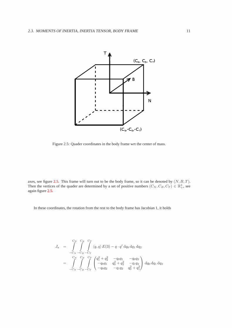
Figure 2.5: Quader coordinates in the body frame wrt the center of mass.
axes, see figure2.5. This frame will turn out to be the body frame, so it can be denoted by(N, B, T ).Then the vertices of the quader are determined by a set of positive numbers(CN , CB, CT ) ∈ R3
+, seeagain figure2.5.
In these coordinates, the rotation from the rest to the body frame has Jacobian 1, it holds
Ja =
CN∫
−CN
CB∫
−CB
CT∫
−CT
〈q, q〉E(3) − q · qt dq0 dq1 dq2
=
CN∫
−CN
CB∫
−CB
CT∫
−CT
q21 + q2
2 −q0q1 −q0q2
−q0q1 q20 + q2
2 −q1q2
−q0q2 −q1q2 q20 + q2
1
dq0 dq1 dq2
12 CHAPTER 2. THE SPINNING TOP
Evaluating fori 6= j 6= k 6= i
CN∫
−CN
CB∫
−CB
CT∫
−CT
(q2i + q2
j ) dq0dq1dq2 = 8 ·CN∫
0
CB∫
0
CT∫
0
(q2i + q2
j ) dq0dq1dq2
= 8 · Ck
Cj∫
0
[13q3i + qiq
2j
]Ci
qi=0dqj
= 8 · Ck · Ci
Cj∫
0
(C2
i
3+ q2
j ) dqj
= 8 · Ck · Ci
[C2i
3qj +
1
3q3j
]Cj
qj=0
=8 · CN · CB · CT
3(C2
i + C2j )
and
CN∫
−CN
CB∫
−CB
CT∫
−CT
(−qiqj) dq0dq1dq2 = 2 · Ck
Cj∫
−Cj
[− 1
2q2i qj
]Ci
qi=−Ci
dq0 dqj
= 2 · Ck
Cj∫
−Cj
(− 1
2C2
i qj +1
2C2
i qj
)dq0 dqj
= 0
gives
Ja =M3
CB2 + CT
2 0 0
0 CN2 + CT
2 0
0 0 CN2 + CB
2
.
The fact thatJa is already diagonal in the frame(N, B, T ) shows that this is indeed the body framewrt the center of mass. The mass of the quaderM = 8 · CN · CB · CT can be immediately seen fromfigure2.5, since it has unit density.
An example for such a body frame of a quader visualized in theTop Visualizationprogram can beseen in figure2.6.
Now a summary of notations:
Definition (Notations). The coordinates of the vertices of the quader in the body frame are determinedby a set of positive numbers(CN , CB , CT ) ∈ R3
+. This set will be called thecoordinates of the quaderor quader coordinates. See figure2.5. Coordinates of vectors wrt the restframe will get small letters, wrtthe bodyframe big ones, e. g.

2.3. MOMENTS OF INERTIA, INERTIA TENSOR, BODY FRAME 13
Figure 2.6: Body frame wrt the center of mass of a quader.
(N, B, T ) the body frame(e1, e2, e3) the rest frame
q radius vector of a point in the rest frameQ radius vector of a point in the body frameω vector of angular velocity in the rest frameΩ vector of angular velocity in the body framem vector of angular momentum in the rest frameM vector of angular momentum in the body framep gravity vector in the rest frame (p is constant)P gravity vector in the body frame
M the mass of the bodyIi (principal) moment of inertia wrt the axis spanned byei
The results so far are useful for rotations around the centerof mass. For arbitrary fixed points oneneeds the inertia tensor at an arbitrary point. But this is easily calculated with the following two state-ments.
Theorem 2.4(Parallel axes theorem or Huygens-Steiners theorem). Let l be an axis passing through thecenter of massa of a body ands an axis parallel tol, then the moments of inertia of the body wrt thoseaxes satisfy
Is = Il + M · d2 (2.12)
whered is the distance between thel ands axes, see figure2.7(a).
Proof. By the law of cosinesr2s(q) = d2 + r2
l (q) − 2d rl(q) cos φ
whererl(q) is the distance ofq to l, rs(q) the distance ofq to s andφ the angle like in figure2.7(b).

14 CHAPTER 2. THE SPINNING TOP
(a) Viewed in a plane spanned by the axes. (b) Viewed in a plane perpendicular to the axes.
Figure 2.7: Body with two parallel rotation axes.
Hence
Is =
∫
V
ρ(q) r2s(q) dq
=
∫
V
ρ(q) d2 dq +
∫
V
ρ(q) r2l (q) dq − 2
∫
V
ρ(q) d rl(q) cosφdq
= d2
∫
V
ρ(q) dq +
∫
V
ρ(q) r2l (q) dq − 2d
∫
V
ρ(q) rl(q) cosφdq
= M · d2 + Il − 2d
∫
V
ρ(q) rl(q) cosφdq
So it suffices to show that ∫
V
ρ(q) rl(q) cos φdq = 0 (2.13)
By definition of the center of mass,
a =1
M
∫
V
ρ(q) q dq.
Choosing a coordinate system with the origin at the center ofmassa andl pointing inz-direction, furtherexpressingq in cylindrical coordinates, one gets
0 =
∫
V
ρ(q)
rl cosφrl sin φ
z
dq
whose first coordinate is the desired equation (2.13).
Corollary 2.5. Let a be the center of mass of a rigid body andJa its inertia tensor,p another pointdisplaced froma by the vector~r andJp the body’s inertia tensor wrtp. Then
Jp = Ja + M(〈~r, ~r〉E(3) − ~r · ~rt
)(2.14)

2.3. MOMENTS OF INERTIA, INERTIA TENSOR, BODY FRAME 15
Figure 2.8: Inertia tensor wrt the center of mass and a secondpoint p.
whereE(3) is the 3x3 unit matrix. See figure2.8.
Proof. The moment of inertia of the body wrt the axis through the center of massa pointing in thedirection of a unit vector~w is
I~w,a = 〈~w, Ja ~w〉 .
By the parallel axes theorem,I~w,p = I~w,a + M· d2.
Now,d2 = 〈~r, ~r〉 − 〈~r, ~w〉2
and hence
〈~w, Jp ~w〉 = 〈~w, Ja ~w〉 + M(〈~r, ~r〉 − 〈~r, ~w〉 〈~r, ~w〉
)
= 〈~w, Ja ~w〉 + M(〈~r, ~r〉 〈~w, ~w〉 − 〈~w, 〈~r, ~w〉~r〉
)
= 〈~w, Ja ~w〉 + M(〈~w, 〈~r, ~r〉 ~w〉 −
⟨~w,~r · ~rt ~w
⟩ )
=⟨
~w,[Ja + M
(〈~r, ~r〉E(3) − ~r · ~rt
)]~w⟩
Corollary 2.6. For a quader with quader coordinates(CN , CB , CT ) in body frame(N, B, T ) attachedto the center of mass, the point with coordinates(0, 0,−CT ) lies on the center of one of the quader faces.The inertia tensor of the quader wrt this point is
J =M3
CB2 + (2CT )2 0 0
0 CN2 + (2CT )2 0
0 0 CN2 + CB
2
.

16 CHAPTER 2. THE SPINNING TOP
Proof. It is clear that the point lies at the center of a quader face. For the inertia tensor one gets with thepreceding corollary
J = Ja + M(〈~r, ~r〉E(3) − ~r · ~rt
)
=M3
CB2 + CT
2 0 0
0 CN2 + CT
2 00 0 CN
2 + CB2
+ M
(C2
T · E(3) −
0 0 00 0 00 0 C2
T
)
=M3
CB2 + (2CT )
20 0
0 CN2 + (2CT )
20
0 0 CN2 + CB
2
SinceJ stayed diagonal, the body frame stays the same, but is just attached to the new fixed point(0, 0,−CT ). See again figure2.4. In theTop Visualizationprogram this point is the fixed point and thisinertia tensor the one relevant for the body motion.
2.4 The Lagrange top
Definition. A Lagrange topis a spinning top which is symmetric wrt a rotation4 around an axis throughthe fixed point.
Remark.The rotational symmetry implies that the center of mass of the body lies on the symmetry axis.Would it lie elsewhere it would move during the rotation and the body could not be the same as before.
The Lagrange top is an interesting case of rigid body motion since it is integrable. More about thatwill follow in the next chapter.
Example.A homogeneous5 quader with coordinates(CN , CN , CT ) is mapped to itself by a rotation bythe angleπ/2 aroundT , the third axis of the body frame. Hence, if the fixed point lies on that axis, thequader is a Lagrange top. See figure2.9.
The Lagrange top visualized in theTop Visualizationprogram has the fixed point at−CT · T whichis (0, 0,−CT ) in body frame coordinates.
4The body is mapped to itself by a rotation by2π/n for ann > 2.5Constant density function.

2.4. THE LAGRANGE TOP 17
Figure 2.9: A Lagrange top.

18 CHAPTER 2. THE SPINNING TOP

Chapter 3
Dynamics
In this section the (continuous) equations of motion of a spinning top in the rest frame1 are derived.Therefore the necessary variational principals and the energy of the spinning top are recalled. For asimplification of calculations an isomorphism betweenR3 and the matrix groupsu(2) as well as themotion groupSO(3) andSU(2) are introduced.
Further the analogies between Lagrange tops and elastic curves (Kirchhoffs analogy) as well as spin-ning tops and elastic rods are presented. The former served as the guiding idea for finding an integrablediscretization of the Lagrange top, as described in [BS00] and implemented in theTop Visualizationprogram.
3.1 Variational principals
Definition. Let
L : Rn × R
n × [t0, t1] −→ R
(p, q, t) 7−→ L(p, q, t)
be a twice differentiable functional. Then a twice differentiable curve
f : [a, b] 7−→ Rn
is called anextremal of the functional
S(f) =
t1∫
t0
L(f(t), f ′(t), t) dt
if it minimizes S over the set of all twice differentiable funtions on[t0, t1] with the same values asf att0 andt1.
Theorem 3.1(Hamilton’s principal of least action). Motions of mechanical systems2 coincide with ex-tremals of the functional
S(f) =
t1∫
t0
L(f(t), f ′(t), t) dt,
1The equations of motion in the body frame are the well known Kirchhoff equations, but a rest frame formulation will proveuseful for finding a numerical solution.
2Systems in which Newtons equations of motion hold.
19
20 CHAPTER 3. DYNAMICS
where
L = T − U
is the difference between the kinetic and the potential energy, the so calledLagrange functionor La-grangian.
Proof. Omitted. See e. g. [Arn].
Definition. A variationof a curvef : [t0, t1] → Rn, t 7→ f(t) is a twice differentiable function
fε : [t0, t1] × [−ǫ, ǫ] −→ Rn
(t, ε) 7−→ fε(t, ε)
that satisfies
fε(t, 0) = f(t) ∀t ∈ [t0, t1],
fε(t0, ε) = f(t0) ∀ε ∈ [−ǫ, ǫ]
and
fε(t1, ε) = f(t1) ∀ε ∈ [−ǫ, ǫ].
Lemma 3.2. An extremalf(t) of a functionalS(f) satisfies
0 =d
dε
t1∫
t0
L(fε(t, ε), f′
ε(t, ε), t) dt
∣∣∣∣∣ε=0
for all variationsfε of f .
Proof. Omitted. See e. g. [Arn].
Lemma 3.3(Fundamental lemma of calculus of variations). If a continuous functionf : [t0, t1] → R
satisfiest1∫
t0
f(t)h(t) dt = 0
for all continuous functionh(t) with h(t0) = h(t1) = 0, then
f(t) ≡ 0.
Proof. Omitted. See e. g. [Arn].
Remark.With the stated principals one can already find the equationsof motion of a spinning top. Thefunctionf is the position of the top at timet, i. e. the rotation from the rest frame to the body frame.But dealing with rotations is much more convenient in the LiegroupSU(2) and its Lie algebrasu(2)compared to the rotation groupSO(3) andso(3). The isomorphism between them is introduced in shortin the next chapter, for more details see [B06].
3.2. ROTATION INR3, SU(2) AND SU(2) 21
3.2 Rotation in R3, su(2) and SU(2)
3.2.1 The vector spacesu(2)
The set of skew symmetric complex two by two matrices with trace zero
su(2) := A ∈ gl(2, C), A∗ = −A, tr(A) =)is a vector space and
e1 =1
2
(0 −i−i 0
), e2 =
1
2
(0 −11 0
), e3 =
1
2
(−i 00 i
)
a basis3 of su(2), since
A =
(a bc d
)a, b, c, d ∈ C
⇒ A∗ = −A ⇔ a = −a, d = −d, b = −c andc = −b
⇔ A =
(iα b−b iδ
), α, δ ∈ R
tr(A) = 0 ⇔ α = −δ
⇒ A ∈ su(2) ⇔ A =
(iα β + iγ
−β + iγ −iα
)= −2γe1 − 2βe2 − 2αe3 α, β, γ ∈ R.
This gives an isomorphism betweenR3 andsu(2). I. e. a vectorx = (x1, x2, x3) is identified with
the matrixx = 12
(−ix3 −x2 − ix1
x2 − ix1 ix3
)and all operations inR3 can as well be carries out with the
corresponding operations insu(2). From now on the same notations will be used for vectors inR3 andtheir correspondingsu(2) matrices.
The scalar product induced fromR3 can be calculated as
〈x, y〉 = −2tr(xy),
since then
〈e1, e1〉 = −2tr
(1
2
(0 −i−i 0
)· 1
2
(0 −i−i 0
))
= −2tr
(1
4
(−1 00 −1
))
= 1
and similar〈e2, e2〉 = 〈e3, e3〉 = 1
as well as
〈e1, e2〉 = −2tr
(1
4
(0 −i−i 0
)·(
0 −11 0
))
= −2tr
(1
4
(−i 00 i
))
= 03This basis was chosen in such a way, that the matrix commutator will correspond to the cross product.

22 CHAPTER 3. DYNAMICS
and similar〈e2, e3〉 = 〈e1, e3〉 = 0.
Defining the matrix commutator
[x, y] := xy − yx x, y ∈ su(2),
then the corresponding vectors satisfyx × y = [x, y].
Proof.
[x, y] = xy − yx
=1
2
(−ix3 −x2 − ix1
x2 − ix1 ix3
)1
2
(−iy3 −y2 − iy1
y2 − iy1 iy3
)
−1
2
(−iy3 −y2 − iy1
y2 − iy1 iy3
)1
2
(−ix3 −x2 − ix1
x2 − ix1 ix3
)
=1
4
(−x3y3 − x2y2 − x1y1 − i(x1y2 − x2y1) −(x3y1 − x1y3) − i(x2y3 − x3y2)
(x3y1 − x1y3) − i(x2y3 − x3y2) −x3y3 − x2y2 − x1y1 + i(x1y2 − x2y1)
)
−1
4
(−x3y3 − x2y2 − x1y1 + i(x1y2 − x2y1) (x3y1 − x1y3) + i(x2y3 − x3y2)
−(x3y1 − x1y3) + i(x2y3 − x3y2) −x3y3 − x2y2 − x1y1 − i(x1y2 − x2y1)
)
=1
2
(−i(x1y2 − x2y1) −(x3y1 − x1y3) − i(x2y3 − x3y2)
(x3y1 − x1y3) − i(x2y3 − x3y2) i(x1y2 − x2y1)
)
vector
form=
x2y3 − x3y2
x3y1 − x1y3
x1y2 − x2y1
= x × y
Further note that
eiej =1
2εijkek (3.1)
whereεijk is the totally antisymmetric tensor withε012 = 1.
3.2.2 The matrix groupSU(2)
The set of unitary two by two matricis with determinant one
SU(2) := A ∈ gl(2, C), A∗A = Id, det(A) = 1
is a matrix group, with which rotations inR3 can be conveniently described:
Theorem 3.4. A vectorX ∈ R3 rotated around a unit vector4 V ∈ R3, 〈V, V 〉 = 1 by the angleα ∈ R
can be described in terms ofsu(2) andSU(2) as
X 7→ Φ−1XΦ ∈ su(2),
whereSU(2) ∋ Φ = cos α2 · Id(2) + sin α
2 V . Φ, Φ ∈ SU(2) describe the same rotation if and only if
they satisfyΦ = ±Φ.
4Or more precisely around the axis through the origin spannedby V .

3.2. ROTATION INR3, SU(2) AND SU(2) 23
Proof. Omitted here, see e. g. [B06].
Theorem 3.5. LetF = (N, B, T ) : [t0, t1] → SO(3) be a differentiable motion5 in R3, then
1. there exists a differentiableΦ : [t0, t1] → SU(2) with
N ↔ Φ−1e1Φ
B ↔ Φ−1e2Φ
T ↔ Φ−1e3Φ.
2. Φ : [t0, t1] → SU(2) is unique up to the transformationΦ 7→ −Φ.
3. Φ satisfiesΦ′ = UΦ whereU = κ2e1 − κ1e2 − τe3 ∈ su(2) and
κ1 := 〈T ′, N〉 is the geodesic curvature,
κ2 := 〈T ′, B〉 the normal curvature and
τ := 〈N ′, B〉 the torsion
of the frame.
Proof. Only 3. will be proved here. Define thereforeU := Φ′Φ−1 and show firstU ∈ su(2). For everyinvertible operator holds
ΦΦ−1 = Iddiff.⇒ Φ′Φ−1 + Φ(Φ−1)′ = 0
⇒ (Φ−1)′ = −Φ−1Φ′Φ−1,
together with
Φ ∈ SU(2) ⇒ Φ∗ = Φ−1
yields
(Φ′Φ−1)∗ = (Φ−1)∗(Φ′)∗
= Φ(Φ′)−1
= Φ(Φ−1)′
= −ΦΦ−1Φ′Φ−1
= −Φ′Φ−1.
Further using
t 7→ A(t), A(t0) = Id ⇒ d
dtdetA(t)
∣∣∣∣∣t=t0
= tr(A′(t0))
one gets
tr(Φ′Φ−1) =d
dtdet(Φ(t)Φ−1(t0))
∣∣∣∣∣t=t0
=d
dtdet(Φ(t))︸ ︷︷ ︸
=1
det(Φ−1(t0))︸ ︷︷ ︸=const.
∣∣∣∣∣t=t0
= 05(N, B, T ) is a positive oriented orthonormal basis∀t ∈ [t0, t1].

24 CHAPTER 3. DYNAMICS
andU ∈ su(2). ThereforeU = a · e1 + b · e2 + c · e3 with
a = 〈U, e1〉b = 〈U, e2〉c = 〈U, e3〉 .
But
κ1 = 〈T ′, N〉=
⟨(Φ−1e3Φ)′, Φ−1e1Φ
⟩
= −2tr((Φ−1e2Φ
′ + (Φ−1)′e2Φ)Φ−1e1Φ)
= −2tr(Φ−1e3Φ′Φ−1e1Φ − Φ−1Φ′Φ−1e3e1Φ)
tr(B−1AB)=tr(A)= −2tr(e3Ue1 − Ue3e1)
tr(AB)=tr(BA)= −2tr(Ue1e3 − Ue3e1)
3.1= −2tr(−U
e2
2− U
e2
2)
= 2tr(Ue2)
= −〈U, e2〉= −b
and similarκ2 = a, τ = −c
and thereforeU = κ2e1 − κ1e2 − τe3.
Lemma 3.6. Let (N, B, T ) : [t0, t1] 7→ SO(3) andΦ : [t0, t1] 7→ SU(2) be corresponding rotations asabove,Ω its vector of angular velocity in the body frame andω in the rest frame, then
Ω = −Φ′Φ−1 (3.2)
ω = −Φ−1Φ′ (3.3)
Proof. On the one hand by definition
N ′ = ω × N = [ω, N ],
on the other hand
N ′ = (Φ−1e1Φ)′
= −Φ−1Φ′Φ−1e1Φ + Φ−1e1Φ′
= Φ−1e1ΦΦ−1Φ′ − Φ−1Φ′Φ−1e1Φ
= [Φ−1e1Φ, Φ−1Φ′] = [N, Φ−1Φ′]
= [−Φ−1Φ′, N ],
which shows3.3. SinceΩ = ΦωΦ−1, see theorem3.4part 1., we immediately get3.2.
3.3. ENERGY OF THE SPINNING TOP 25
3.3 Energy of the spinning top
By corollary2.11the kinetic energy of a rigid body fixed at0 is
T =1
2〈ω, Jrestframe · ω〉 .
Since the scalar product does not change under a rotation thekinetic energy expressed in the body frameis
T =1
2〈Ω, JΩ〉 .
whereΩ is the vector of angular velocity andJ the inertia tensor in the body frame(N, B, T ), i. e.
J =
IN 0 00 IB 00 0 IT
with IN , IB , IT the principal moments of inertia. Therefore
T =1
2(INΩ2
N + IBΩ2B + IT Ω2
T ).
The potential energy of the body isU = M· g · h
whereM is the total mass of the body,g the gravity constant andh the height of the center of massa ofthe body6.
Given a gravity vectorp pointing in the (positive) third coordinate direction of the rest frame andhaving lengthg
p = g · e3,
further given the center of mass
a = AN · N + AB · B + AT · T= a1 · e2 + a2 · e3 + a3 · e3, (3.4)
((e1, e2, e3) being the rest frame), one gets
U = M· 〈p, a〉 = M· g · a3.
Finally the Lagrange function is
L = T − U =1
2(INΩ2
N + IBΩ2B + IT Ω2
T ) −M · 〈p, a〉 . (3.5)
3.4 Equation of motion of the spinning top in the rest frame
Let the position of the quader beΦ : [t0, t1] → SU(2), t 7→ Φ(t), then a variation of the position is
Φ : [t0, t1] × [−ǫ, ǫ] −→ SU(2)
(t, ε) 7−→ Φε(t, ε) := Φ(t)H(t, ε)
6The homogeneous gravity field acts on the body as if the body had all its mass concentrated at the center of mass.
26 CHAPTER 3. DYNAMICS
where
H : [t0, t1] × [−ǫ, ǫ] −→ SU(2)
is differentiable and satisfies
H(t0, ε) = H(t1, ε) = H(t, 0) = Id ∀t, ε. (3.6)
Under the variation only the body frame- and rest frame coordinates change. Giving proper notationsand expressing the Lagrange function in body frame coordinates one gets
Lε =1
2(INΩ2
Nε,ε + IBΩ2Bε,ε + IT Ω2
Tε,ε) −M · 〈p, aε〉
=1
2(IN 〈ωε, Nε〉2 + IB 〈ωε, Bε〉2 + IT 〈ωε, Tε〉2)
−M · 〈p, AN · Nε + AB · Bε + AT · Tε〉
=
⟨(1
2IN 〈ωε, Nε〉ωε −M · AN · p
), Nε
⟩
+
⟨(1
2IB 〈ωε, Bε〉ωε −M · AB · p
), Bε
⟩
+
⟨(1
2IT 〈ωε, Tε〉ωε −M · AT · p
), Tε
⟩
(3.7)
By theorem3.1and lemma3.2the motion of the spinning top satisfies
0 =d
dε
t1∫
t0
Lε dt
∣∣∣∣∣ε=0
(3.8)
which is to be calculated in this chapter.
But first some observations. Denote
η :=∂H(t, ε)
∂ε
∣∣∣∣∣ε=0
,
then from theorem3.5and equation (3.6) follows η ∈ su(2).
Further it follows from (3.6) that
η(t0) = η(t1) = 0,
H ′
∣∣∣ε=0
= 0
and
∂H−1
∂ε
∣∣∣ε=0
= −η.

3.4. EQUATION OF MOTION OF THE SPINNING TOP IN THE REST FRAME 27
With that one gets for the variation of the vector of angular velocity
ωε3.3= −Φ−1
ε Φ′
ε
= −(ΦH)−1(ΦH)′
= −H−1Φ−1(Φ′H + ΦH ′)
= H−1(−Φ−1Φ′)H − H−1H ′
= H−1ωH − H−1H ′
⇒ ∂ωε
∂ε=
(H−1ω
∂H
∂ε+
∂H−1
∂εωH − ∂H−1
∂εH ′ − H−1 ∂H ′
∂ε
)∣∣∣∣∣ε=0
= ωη − ηω − η′
= [ω, η] − η′.
Furthermore
Nε = Φ−1ε e1Φε
= H−1Φ−1e2ΦH
= H−1NH
⇒ ∂Nε
∂ε
∣∣∣∣∣ε=0
=
(H−1N
∂H
∂ε+
∂H−1
∂εNH
)∣∣∣∣∣ε=0
= [N, η]
and analog
∂Bε
∂ε
∣∣∣∣∣ε=0
= [B, η],∂Tε
∂ε
∣∣∣∣∣ε=0
= [T, η].
Now equation (3.8) can be solved. The calculation is carried out for theN -component of the Lagrange
28 CHAPTER 3. DYNAMICS
function, the others are analog.
0 =d
dε
t1∫
t0
⟨(1
2IN 〈ωε, Nε〉ωε −M · AN · p
), Nε
⟩dt
∣∣∣∣∣ε=0
=
t1∫
t0
⟨d
dε
(1
2IN 〈ωε, Nε〉ωε −M · AN · p
), Nε
⟩+
⟨(1
2IN 〈ωε, Nε〉ωε −M · AN · p
),
d
dεNε
⟩dt
∣∣∣∣∣ε=0
=
t1∫
t0
⟨1
2IN
(〈ωε, Nε〉
d
dεωε +
⟨d
dεωε, Nε
⟩ωε +
⟨ωε,
d
dεNε
⟩ωε
), Nε
⟩ ∣∣∣∣∣ε=0
+
⟨(1
2IN 〈ω, N〉ω −M · AN · p
), [N, η]
⟩dt
=
t1∫
t0
⟨1
2IN
(〈ω, N〉 ([ω, η] − η′) + 〈[ω, η] − η′, N〉ω + 〈ω, [N, η]〉ω, N
⟩+
1
2IN 〈ω, N〉 〈[η, ω], N〉 − 〈M · AN · [p, N ], η〉 dt
=
t1∫
t0
1
2IN 〈ω, N〉
(〈[ω, η], N〉 − 〈η′, N〉 + 〈[ω, η], N〉 − 〈η′, N〉 + 〈[η, ω], N〉 +
〈[η, ω], N〉)− 〈M · AN · [p, N ], η〉 dt
=
t1∫
t0
〈IN 〈ω, N〉N,−η′〉 dt −t1∫
t0
〈M · AN · [p, N ], η〉 dt
part. Int.= 〈IN 〈ω, N〉N,−η〉
∣∣∣t1
t0+
t1∫
t0
⟨IN
(〈ω, N〉N ′ + 〈ω′, N〉N + 〈ω, N ′
︸︷︷︸=ω×N
〉N), η
⟩dt
−t1∫
t0
〈M · AN · [p, N ], η〉 dt
η(t0)=η(t1)=0=
t1∫
t0
⟨IN (〈ω, N〉N ′ + NN t · ω′) −M · AN · [p, N ], η
⟩dt
In the vector form this is
0 =
t1∫
t0
⟨IN (〈ω, N〉N ′ + NN t · ω′) −M · AN · p × N, η
⟩dt.
Since the direction of variationη is arbitrary one can use lemma3.3and gets
0 = IN (〈ω, N〉N ′ + NN t · ω′) −M · AN · p × N.

3.4. EQUATION OF MOTION OF THE SPINNING TOP IN THE REST FRAME 29
Including all three coordinates this gets
0 = IN (〈ω, N〉N ′ + NN t · ω′) + IB(〈ω, B〉B′ + BBt · ω′) + IT (〈ω, T 〉T ′ + TT t · ω′)
−M · p × (AN · N + AB · B + AT · T )
= (︷ ︸︸ ︷IN · NN t + IB · BBt + IT · TT t
=:A)ω′ + IN 〈ω, N〉ω × N
+IB 〈ω, B〉ω × B + IT 〈ω, T 〉ω × T −M · p × a
⇔ Aω′ = (IN · NN t + IB · BBt + IT · TT t)ω × ω + M· p × a
⇔ ω′(∗)= A−1(Aω × ω + M· p × a) (3.9)
This is the desired equation of motion of the spinning top andtogether with (by definition)
N ′ = ω × N, B′ = ω × B, B′ = ω × B
solved numerically and visualized in theTop Visualizationprogram.In (∗) was used that:
Lemma 3.7. A is invertible.
Proof. Let v ∈ R3\0 arbitrary. Then, withIN , IB, IT > 0,
vT Av = INvT NNT v + IBvT BBT v + IT vT TT T v
= IN (
3∑
i=1
Nivi)2 + IB(
3∑
i=1
Bivi)2 + IT (
3∑
i=1
Tivi)2
= IN 〈v, N〉2 + IB 〈v, B〉2 + IT 〈v, T 〉2
= INv2N + IBv2
B + IT v2T
> 0.
HenceA is positive definite and invertible.
Remark.Another form of equations of motion of a rigid body around a fixed point are Kirchhoffs equa-tions
M = M × (J−1M) + M · P × A
P = P × (J−1M),
where all vectors are expressed in the body frame.For computing numerical solutions, using them has a seriousdisadvantage. When e. g. approximating
a solution at timet+ ε based on given initial data at timet, numerical algorithms evaluate the differentialequations at multiple points within the interval[t, t + ε]. In body frame formulation, the frame staysconstant and can be integrated to the new body frame at timet+ε just usingω(t). The present knowledgeaboutM and henceω at the additional points within the interval[t, t + ε] is lost.
This can be improved by a formulation of the equations of motion in rest frame coordinates, so theycan be solved simultaneously with the motion of the body frame expressed in the rest frame. I. e. solvingthe first order system of ordinary differential equations
ω′ = A−1(Aω × ω + M· p × a)
N ′ = ω × N
B′ = ω × B
T ′ = ω × T
30 CHAPTER 3. DYNAMICS
simultaneously yields far better results, even though the integrability of the last three equations is notused by numerical methods.
3.5 Elastic curves and spinning tops
Definition. A framed curveis an immersed7, arclength parametrized8 curveγ : [0, L] → R3 with a unit
normalfieldN : [0, L] → S2. (N, B := T × N, T := γ′) is the (orthonormal) frame of the curve.Denote the values
κ1 := 〈T ′, N〉 geodesic curvature
κ2 := 〈T ′, B〉 normal curvature
τ := 〈N ′, B〉 torsion.
Definition. A framed curveγ delivering an extremal
• to the functional
S =
L∫
0
κ21 + κ2
2 + ατ2 dx,
is called anisotropic elastic curveor isotropic elastic rod,
• to the functional
S =
L∫
0
α1κ21 + α2κ
22 + ατ2 dx,
is called ananisotropic elastic curveor anisotropic elastic rod,
whereα, α1, α2 ∈ R, the boundary pointsγ(0) andγ(L) and the frames(N, B, T ) at the boundary pointsare fixed.
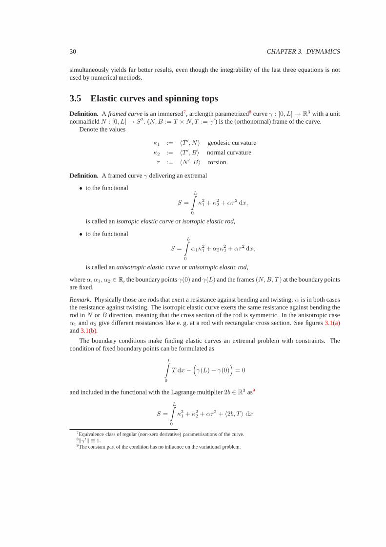
Remark.Physically those are rods that exert a resistance against bending and twisting.α is in both casesthe resistance against twisting. The isotropic elastic curve exerts the same resistance against bending therod in N or B direction, meaning that the cross section of the rod is symmetric. In the anisotropic caseα1 andα2 give different resistances like e. g. at a rod with rectangular cross section. See figures3.1(a)and3.1(b).
The boundary conditions make finding elastic curves an extremal problem with constraints. Thecondition of fixed boundary points can be formulated as
L∫
0
T dx −(γ(L) − γ(0)
)= 0
and included in the functional with the Lagrange multiplier2b ∈ R3 as9
S =
L∫
0
κ21 + κ2
2 + ατ2 + 〈2b, T 〉 dx
7Equivalence class of regular (non-zero derivative) parametrisations of the curve.8‖γ′‖ ≡ 1.9The constant part of the condition has no influence on the variational problem.
3.5. ELASTIC CURVES AND SPINNING TOPS 31
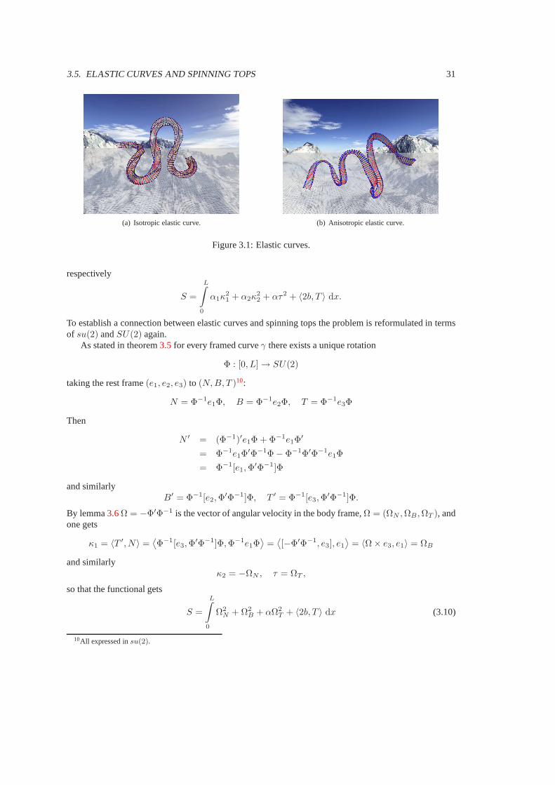
(a) Isotropic elastic curve. (b) Anisotropic elastic curve.
Figure 3.1: Elastic curves.
respectively
S =
L∫
0
α1κ21 + α2κ
22 + ατ2 + 〈2b, T 〉 dx.
To establish a connection between elastic curves and spinning tops the problem is reformulated in termsof su(2) andSU(2) again.
As stated in theorem3.5for every framed curveγ there exists a unique rotation
Φ : [0, L] → SU(2)
taking the rest frame(e1, e2, e3) to (N, B, T )10:
N = Φ−1e1Φ, B = Φ−1e2Φ, T = Φ−1e3Φ
Then
N ′ = (Φ−1)′e1Φ + Φ−1e1Φ′
= Φ−1e1Φ′Φ−1Φ − Φ−1Φ′Φ−1e1Φ
= Φ−1[e1, Φ′Φ−1]Φ
and similarlyB′ = Φ−1[e2, Φ
′Φ−1]Φ, T ′ = Φ−1[e3, Φ′Φ−1]Φ.
By lemma3.6Ω = −Φ′Φ−1 is the vector of angular velocity in the body frame,Ω = (ΩN , ΩB, ΩT ), andone gets
κ1 = 〈T ′, N〉 =⟨Φ−1[e3, Φ
′Φ−1]Φ, Φ−1e1Φ⟩
=⟨[−Φ′Φ−1, e3], e1
⟩= 〈Ω × e3, e1〉 = ΩB
and similarlyκ2 = −ΩN , τ = ΩT ,
so that the functional gets
S =
L∫
0
Ω2N + Ω2
B + αΩ2T + 〈2b, T 〉 dx (3.10)
10All expressed insu(2).

32 CHAPTER 3. DYNAMICS
respectively
S =
L∫
0
α1Ω2N + α2Ω
2B + αΩ2
T + 〈2b, T 〉 dx. (3.11)
So elastic curves deliver an extremals to those functionalswhile the frames at the boundary pointsΦ(0)andΦ(L) are fixed during variation.
But (3.11) is exactly twice the Lagrange function of the spinning top (3.5) if and only if the center ofmass of the topa is parallel toT ; thenb = ‖a‖ · p andα1, α2, α take the roll of the principal moments ofinertia. And since the constant factor2 does not change the extremals of the functional, it holds:
Theorem 3.8. The paths of body frames of spinning tops with the center of mass on one of its principalaxes is in a one-to-one correspondence to frames of anisotropic elastic curves.
Since for the Lagrange topIN = IB anda‖T , (3.10) multiplied by2In gets (3.5) and one has thespecial case of:
Theorem 3.9(Kirchhoffs kinetic analogy). The paths of Lagrange top body frames are in a one-to-onecorrespondence to frames of isotropic elastic curves.
These analogies are visualized in theTop Visualizationprogram as described in section5.7.

Chapter 4
Discretizations
4.1 Numerical discretizations
The path of the spinning top is an ordinary differential equation (ODE), it depends only on time. Innumerical analysis there are various methods of approximating the solutions of ODEs by approximatingits derivatives with the help of finite differences. Depending on the chosen method and the given toleranceparameters, these solutions are more or less accurate. But in general they do not use the fact, that inHamiltonian systems there is an underlying structure that could give more information about the motion.This is one disadvantage of numerical discretizations compared to the integrable discretization describedin the next section.
Further, for a given time discretization step length parameterε, numerical discretizations evaluate theODE several times at points in the interval[t, t + ε], making them much more demanding in terms ofcalculation time and memory.
4.1.1 Extrap - The Gragg-Burlisch-Stoer extrapolation algorithm
In theTop Visualizationprogram described in chapter5 the integrable discretization is compared to theGragg-Burlisch-Stoer extrapolation algorithmthat will be calledExtrapin this thesis and in the program.
The algorithm is based on the explicit midpoint rule with step size control and order selection, see[HNW]. It is a very modern, probably one of the most sophisticatedmethods for solving ODEs.
Error tolerances and step size control Some details of theExtrapmethod from [HNW] are cited herein order to clarify the used error tolerances and the funcionality of the step size control.
Let therefore
y1(t) = f1(y1(t), . . . , yn(t), t)
...
yn(t) = fn(y1(t), . . . , yn(t), t)
be a system ofn ordinary first order differential equations,
h ∈ R+
33

34 CHAPTER 4. DISCRETIZATIONS
be an initial step size length (which may be chosen by the user) and
t0, yi(t0) ∈ R
be the given initial data. Then theExtrapmethod calculates two approximationsy(t0 + h) andy(t0 + h)of y(t0 + h) based on estimation of the derivatives of theyi with the help of finite differences. Then anestimate of the error for the less precise result isy(t0 + h) − y(t0 + h). Now the user wants that error tosatisfy
|y(t0 + h) − y(t0 + h)| ≤ sci, sci := Atoli + max(|y(t0 + h)|, |y(t0 + h)|) · Rtoli.
Relative errors are considered forAtoli = 0, absolute errors forRtoli = 0. Usually both are differentfrom zero in order to have a reasonable error tolerance independant of the values ofyi. As a measure ofthe error theExtrapmethod takes
err =
√√√√ 1
n
n∑
i=1
( y(t0 + h) − y(t0 + h)
sci
)2
.
Then iferr < 1 the step is accepted and a new step size is determined, depending on how smallerr was.For details see [HNW]. If err ≥ 1 the step is rejected and a smaller step size determined, withwhich theresult will probably fulfill the required error tolerances.
When theExtrapmethod is applied to a quader in chapters5 and6 the tolerances are taken equal forall components, i. e.Atoli = Atol, Rtoli = Rtol, ∀i = 1, . . . , n, and alsoAtol = Rtol are taken equal.
4.2 Integrable discretization by A. I. Bobenko and Yu. B. Suris
This section gives an outline of the integrable time discretization of the Lagrange top as derived in [BS00],which will be called theBobenko-Suris discretizationin the present work. The derivations are made in ascaled coordinate system that simplifies certain quantities, this scaling is first demonstrated at the exampleof a quader. Then the used notations are recalled and finally the results that were implemented in theTopVisualizationprogram are cited.
4.2.1 Calculation in a scaled coordinate system
Recalling that in the body frame a Lagrange top with coordinates as desribed in2.5has the inertia tensor1
J =M3
CN2 + (2CT )2 0 0
0 CN2 + (2CT )2 0
0 0 2CN2
,
withM = 8CNCBCT = 8C2
NCT
and center of mass coordinates
A =
00
CT
,
one can simplify those by choosing appropriate units.
1In the Lagrange caseCN = CB .

4.2. INTEGRABLE DISCRETIZATION BY A. I. BOBENKO AND YU. B. SURIS 35
First scaling the length unit (calling the given length unitlu and the scaled onelu) by
1 lu = CT lu
the center of mass has coordinates
A =
001
,
wrt the scaled bodyframe(e1, e2, e3) = CT (e1, e2, e3).The (principal) moments of inertia have the unit[lu2 mu], mu being the mass unit. Thus by scaling
1 mu =8C2
N
3CT
(C2N + C2
T )mu
one gets in scaled coordinates
I1 = I2 =M3
(C2N + C2
T ) lu2 mu
=8C2
NCT
3(C2
N + C2T )(
1
CT
lu)2(3CT
8C2N (C2
N + C2T )
mu)
= 1 lu2mu
and
I3 =M3
(2C2N ) lu2 mu
=2C2
N
C2N + C2
T
lu2mu,
so that in scaled coordinates
J =
1 0 00 1 0
0 02C2
N
C2
N+C2
T
or shorter
J =
1 0 00 1 00 0 α
(4.1)
as used in [BS00].Of course in this new units the vector of angular momentumm (respectivelyM ) and the gravity
vectorp have new coordinates, namely
m =
m0
m1
m2
mu lu2
s2=
3
8C2NCT (C2
N + C2T )
m0
m1
m2
mu lu
2
s2
andM gets the same factor,
p =
00g
lu
s2=
1
CT
00g
lu
s2.
The vector of angular velocityω has the unit1s2 and therefore remains the same.

36 CHAPTER 4. DISCRETIZATIONS
4.2.2 Notations
The calculations in [BS00] are carried out in the Lie groupSU(2) and the Lie algebrasu(2), as describedin section3.2.
Recalled in short, all used vectors inR3 are carried over to elements ofsu(2) by the identification
R3 ∋ x =
x1
x2
x3
↔ 1
2
(−ix3 −x2 − ix1
x2 − ix1 ix3
)∈ su(2).
Rotations inR3 are identified with elements offSU(2) according to theorem3.4.Now the notations used in [BS00] in the body frame2 are
k discrete time index,k ∈ Z
ε discrete time step length
ak center of mass at timek, in scaled units‖ak‖ = 1 ∀kp gravity vector,p = g · e2 = const.
mk vector of angular momentum at timek
gk (rotation from rest- to) body frame at timek1 2 × 2 unit matrix
α anisotropy parameter of the Lagrange top, see (4.1)c c = 〈mk, p〉 integral of motion (like in every homogeneous gravity field)
4.2.3 Results
Now theBobenko-Suris discretizationis given by the following two theorems.
Theorem 4.1. The discrete time evolution of a Lagrange top satisfies
mk+1 = mk + ε[p, ak]
ak+1 = (1 + εmk+1)ak(1 + εmk+1)−1.
Theorem 4.2. The discrete time evolution of the framegk can be determined from the linear differenceequation
gk+1 = wkgk,
where thewk are given by
wk =tr(wk)
2(1 + εξk),
where
ξk = mk+1 + c1 − α
α
ak+1 + ak
1 + 〈ak, ak+1〉
=2
c
[ak, ak+1]
1 + 〈ak, ak+1〉+
c
α
ak+1 + ak
1 + 〈ak, ak+1〉,
and
tr(wk) =2√
1 + ε2
4 〈ξk, ξk〉=
√21 + 〈ak, ak+1〉1 + ε2c2/4α2
.
2Only the results in term of the body frame are used here.

4.2. INTEGRABLE DISCRETIZATION BY A. I. BOBENKO AND YU. B. SURIS 37
This discretization is calculated and visualized in theTop Visualizationprogram described in chapter5.

38 CHAPTER 4. DISCRETIZATIONS

Chapter 5
Calculation and the Top Visualization
This section is devoted to the actual calculation of the top motion and its visualization in theTop Visualizationprogram. It can be found on the CD attached to the back cover orun-der http://www.math.tu-berlin.de/˜bodack. It is also available as webstart application underhttp://www.math.tu-berlin.de/geometrie/ps/software.shtml. 1
5.1 JReality
The Top Visualizationprogram uses the jReality software [TBa], a 3D viewer in which the observercontrols an avatar moving in a virtual environment and interacts with its content.
5.2 Move, look around, open panels
Move W, A, S, D.Look around Hold the right mouse button and move the mouse.
Jump SPACE.Toggle gravity2 G.
VR settings panel Doubleclick with the left mouse button on the scene floor. Seesection5.3.Top Visualization panel Doubleclick with the left mouse button on the spinning top. See section5.6.
5.3 Change jReality configuration
JReality configuration can be changed in theVR settingspanel, see figure5.1. It is opened with a dou-bleclick on the scene floor.
A detailed description of JReality can be found atwww.jreality.de, in particular in the containedWiki.
1Note that JavaTM Vs. 1.5 or higher is required. Also the program is rather intense in graphics and calculation, making it hard touse on slow systems.
2Not related to the gravity accelerating the top.
39

40 CHAPTER 5. CALCULATION AND THE TOP VISUALIZATION
(a) Object position. (b) Scene background. (c) Object appearance.
Figure 5.1: JReality configurations.
5.3.1 2D view of the scene
One special option to change the view of the scene is includedin theTop Visualization panel, see figure5.2. The checkboxview scene in (nearly) 2Dsets the position of the observer away from the object andincreases the zoom factor. This way the contortion occurring in a 3D viewer is diminished.
5.4 Loaded content: A Lagrange top example
At startup the program loads a Lagrange top example like described in chapter2, namely a quader withfixed point at the center of one of its faces and quader coordinates(CN , CN , CT ). See e. g. figure2.5foran explanation of these coordinates. TheTop Visualization panelshould be loaded and visible, too.
5.5 A first test run, the buttons Start/Stop and Step
Klick the Stepor theStart/Stopbutton. TheStepbutton makes the program calculate a single motion step,whereas theStart/Stopbutton starts a timer letting the program calculate the nextstep after every certaintime period. This period is an internally stored variable called delay which is indirectly editable with thespeedslider described later in this chapter. Details of the used timer are given in section5.8.5.
5.6 Change top and motion settings
The parameters of the top and its motion can be changed in theTop Visualization panel, see figure5.2.Also various statistics are shown, depending on the loaded content.
5.6.1 Rotate quader
Left click, hold and drag the quader faces or edges.The resulting rotation changes in the initial body frame, but keeps the quader coordinates.
5.6.2 Change size
Left click, hold and drag one of the points that are not at a corner of the face with the fixed point.

5.6. CHANGE TOP AND MOTION SETTINGS 41
Figure 5.2: TheTop Visualization panel. Here the parameters of the top and its motions can be set andvarious statistics are shown.
This changes the quader coordinates(CN , CB , CT ) in the body frame, see figure2.5, and hence themass
M = 8 · CN · CB · CT
and also the moments of inertia, since the inertia tensor in the body frame is (see corollary2.6)
J =M3
CB2 + (2CT )2 0 0
0 CN2 + (2CT )2 0
0 0 CN2 + CB
2
.
5.6.3 Change fixed point
Click, hold and drag one of the quaders points with the middlemouse button. The origin stays themotions fixed point, the quaders position changes and effectively, seen from the quaders point of view,this corresponds to a quader motion wrt a changed fixed point.
While dragging the quader, the principal axes of inertia (the body frame) and the center of mass ofthe body are shown. See figure5.3.
The principal axes and moments of inertia are calculated with the help of equation (2.14). Eigenvec-tors and Eigenvalues are calculated with the package [MTJ].
Remark.Changing the quaders fixed point is equivalent to changing its center of mass. This way, togetherwith changing the quader coordinates, the geometry of everyrigid body can be set, since it is determinedby the body’s center of mass and moments of inertia.

42 CHAPTER 5. CALCULATION AND THE TOP VISUALIZATION
Figure 5.3: Example for a quader with an arbitrary fixed point. Moving the quader in the scene corre-sponds to changing its fixed point, seen from the quaders point of view.
5.6.4 Edit vector of kinetic momentum
Left click, hold and drag the tip2 of the green vector.
The vector of angular velocity (blue) is automatically updated via formula (2.5).
5.6.5 Epsilon, speed and gravity
Epsilon takes the role of the time discretization step length. E. g. the motion of a system traversingt ∈ [0, 1] with anepsilon = 0.02 is approximated atN = 50 equidistant time points.
Thespeed determines how fast the quader in the program should move. Effectively it sets a parameter
delay =1000ε
speedms
of the timer described in section5.8.5and lets the program calculate a motion step more or less often.
The implementation of the timer allows onlydelay ∈ N, which is assured by only accepting certainvalues forspeed. The details are omitted here.
Thegravityslider sets the length of the gravity vector, which points upin the scene, or ine3-directionof the rest frame. (It is not visible in theTop Visualizationprogram.) The higher the gravity the more thebody is accelerated in negativee3-direction.
2The point that is not the fixed point.

5.6. CHANGE TOP AND MOTION SETTINGS 43
5.6.6 The Kowalewski and Goryachev-Chaplygin cases
Activating the corresponding checkbox edits the current quader such that it becomes a Kowalewski re-spectively Goryachev-Chaplygin case of rigid body motion.These are further3 integrable spinning topcases:
Definition. The Kowalewski case is characterized by the principal moments of inertia satisfingI1 = I2 = 2I3 and the center of mass lying in the plane spanned by the principal axes corresponding toI1 andI2.
In the Goryachev-Chaplygincase the center of mass lies in the same plane, the principal momentsof inertia satisfyI1 = I2 = 4I3 and additionally the vector of kinetic momentum is perpendicular to thegravity vector (or alternatively the third component of thevector of kinetic momentum in the rest framem3 is zero).
Denoting again the vector of angular momentum asM = (M1, M2, M3) and the gravity vector asp = (p1, p2, p3), then with appropriately scaled units the Hamiltonian4 is in theKowalewskicase
H =1
2(M2
1 + M22 + 2M2
3 ) − p1
and has the additional integral
K = (M21 − M2
2 + 2p1)2 + 4(M1M2 + p2)
2, (5.1)
in theGoryachev-Chaplygincase
H =1
2(M2
1 + M22 + 4M2
3 ) − 2p1,
which has the additional integral
G = M3(M21 + M2
2 ) + 2M1p3. (5.2)
This and more details can be found in e. g. [BBEIM].
Example.In theTop Visualizationprogram a Kowalewski and a Goryachev-Chaplygin case is constructedfrom a quader with fixed point at the center of one of its faces.In the body frame(N, B, T ) the center ofmass lies on the axis spanned byT , hence i. e. in the plane spanned byB andT .
The quader with quader coordinates(CN , CB , CT ) ∈ R3+ have the principal moments of inertia
I1 =M3
(C2B + (2CT )2), I2 =
M3
(C2N + (2CT )2), I3 =
M3
(C2N + C2
B),
which means for the Kowalewski case
2(C2B + (2CT )2) = C2
N + (2CT )2 = C2N + C2
B
⇔ CT =1
2CB , CN =
√3CB
and for the Goryachev-Chaplygin case
4(C2B + (2CT )2) = C2
N + (2CT )2 = C2N + C2
B
3In the spinning top case there exist four integrable cases. The euler top has the fixed point at the center of mass, the Lagrangetop is described in section2.4and the remaining two cases are described here.
4The Legendre transform of the Lagrangian, i. e.H = T + U , whereT is the kinetic andU the potential energy.

44 CHAPTER 5. CALCULATION AND THE TOP VISUALIZATION
(a) A Kowalewski top. (b) A Goryachev-Chaplygin top.
Figure 5.4: Special integrable top cases.
⇔ CT =1
2CB, CN =
√7CB
with the additional condition ofM2 = 0.Hence, by clicking the checkboxes for those cases, justCN andCT are adjusted toCB (and in the
Goryachev-Chaplygin case additionally the vector of angular momentum). For examples see figures5.4(a)and5.4(b).
The corresponding integrals of motion5.1and5.2then appear next to the checkboxes and are recalcu-lated every time a new motion step is performed. The occurring fluctuation is a measure of the exactnessof the used discretization (which is in this case theExtrapmethod).
Example.An exemplary course of the error in the integralK can be seen in figure5.5. Thereby theinitial settings are the settings at startup of theTop visualizationprogram, but with the quader adjustedto a Kowalewski top by clicking theKowalewskicheckbox.ε was0.1 and the error was plotted over aperiod of300 time units.
The integralG in the Goryachev-Chaplygin case shows a similar behaviour.
5.7 Elastic rods and the apex trace
The analogies stated in theorems3.8and3.9can be observed in the mode of arbitrary quaders. Then thetabRod & Apex traceis availiable at which the elastic rod can be activated and configured. See figure5.6.
5.7.1 Kirchhoffs analogy visualized
If the quader is a Lagrange top, Kirchhoffs analogy3.9 is visualized as follows:As described in section3.5 the motion of the Lagrange top body frame is the frame of an isotropic
elastic curve (or rod). Hence, by taking the body frame at every discrete time step, moving it byε5 to thedirection ofT (the third axis of the body frame, which points to the center of mass) and connecting theold and the new origin, one gets a discrete elastic rod.
But since that would move the frame away from the top, the origin is actually kept and instead allformer points moved in negativeT direction byε. This way the same rod appears and stays close to the
5The current time step length.

5.7. ELASTIC RODS AND THE APEX TRACE 45
Figure 5.5: An exemplary error of the Kowalewski integral ofmotionK(t) − K(0). A small error is aquality measure of the used discretization. The total valueof K was in this settings approximately0.5.
Figure 5.6: TheRod & Apex Tracetab of theTop Visualizationpanel.

46 CHAPTER 5. CALCULATION AND THE TOP VISUALIZATION
Figure 5.7: A Lagrange top with its corresponding isotropicelastic rod.
top. See figure5.7. Also remark that the rod has a symmetric cross section, i. e.the bending energy isequal for all bending directions perpendicular toT , so that it really corresponds to a Lagrange top.
5.7.2 Analogy of tops and anisotropic elastic rods visualized
Analogy 3.8 between tops with gravity center on one of its principal axesand anisotropic elastic rodsis visualized for the special cases of Kowalewski- and Goryachev-Chaplygin tops that appear when thecorresponding checkboxes are activated, see figures5.8(a)and5.8(b).
In both of these cases the center of mass lies on a principal axis. This axis and a second one haveidentical moments of inertia; the third axis, in whose direction the quader is stretched out, has halfrespectively quarter the moment of inertia. Accordingly the bending energy of the elastic rod is alsohalf/quarter, when rotating around this axis. This corresponds to a rod with half/quarter the thickness inthe corresponding direction, see again5.8(a)and5.8(b).
5.7.3 The apex trace visualized
The apex trace is the trace of the intersection point of the symmetry axis of a Lagrange top and asphere with the center at the fixed point. It shows two periodic motions, the nutation and precession,see e. g. [Arn]. Nutation is the periodic rise and fall of the apex trace, precession its azimuthal motion,see figure5.9.
In the Top Visualizationprogram one can show the apex trace when in the arbitrary quader mode,but the quader still has to be a Lagrange top (i. e. has coordinates(CN , CN , CT )). Then, if not alreadyactivated, klick theapex tracecheckbox in theRod & Apex tracetab of theTop Visualization panel.

5.7. ELASTIC RODS AND THE APEX TRACE 47
(a) Anisotropic elastic curve from Kowalewski top. (b) Anisotropic elastic curve from Goryachev-Chaplygintop.
Figure 5.8: Anisotropic elastic curves.
Figure 5.9: The apex trace of a Lagrange top, intersection ofthe symmetry axis and a sphere around thefixed point. The nutation is the periodic motion up and down, the precession left and right.
48 CHAPTER 5. CALCULATION AND THE TOP VISUALIZATION
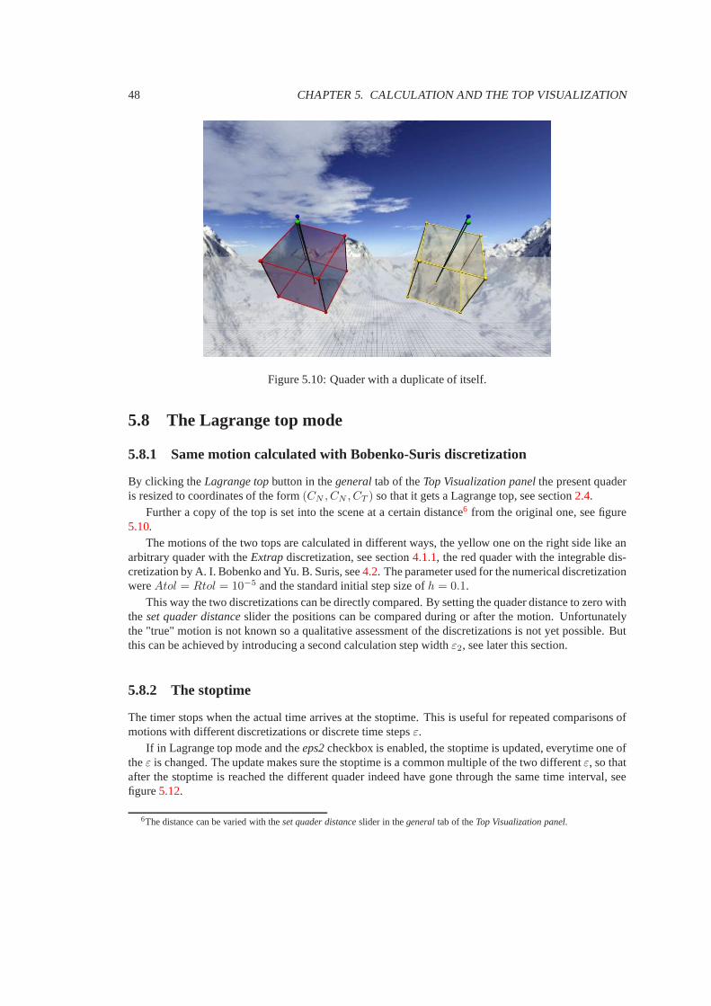
Figure 5.10: Quader with a duplicate of itself.
5.8 The Lagrange top mode
5.8.1 Same motion calculated with Bobenko-Suris discretization
By clicking theLagrange topbutton in thegeneraltab of theTop Visualization panelthe present quaderis resized to coordinates of the form(CN , CN , CT ) so that it gets a Lagrange top, see section2.4.
Further a copy of the top is set into the scene at a certain distance6 from the original one, see figure5.10.
The motions of the two tops are calculated in different ways,the yellow one on the right side like anarbitrary quader with theExtrapdiscretization, see section4.1.1, the red quader with the integrable dis-cretization by A. I. Bobenko and Yu. B. Suris, see4.2. The parameter used for the numerical discretizationwereAtol = Rtol = 10−5 and the standard initial step size ofh = 0.1.
This way the two discretizations can be directly compared. By setting the quader distance to zero withtheset quader distanceslider the positions can be compared during or after the motion. Unfortunatelythe "true" motion is not known so a qualitative assessment ofthe discretizations is not yet possible. Butthis can be achieved by introducing a second calculation step widthε2, see later this section.
5.8.2 The stoptime
The timer stops when the actual time arrives at the stoptime.This is useful for repeated comparisons ofmotions with different discretizations or discrete time stepsε.
If in Lagrange top mode and theeps2checkbox is enabled, the stoptime is updated, everytime oneoftheε is changed. The update makes sure the stoptime is a common multiple of the two differentε, so thatafter the stoptime is reached the different quader indeed have gone through the same time interval, seefigure5.12.
6The distance can be varied with theset quader distanceslider in thegeneraltab of theTop Visualization panel.
5.8. THE LAGRANGE TOP MODE 49
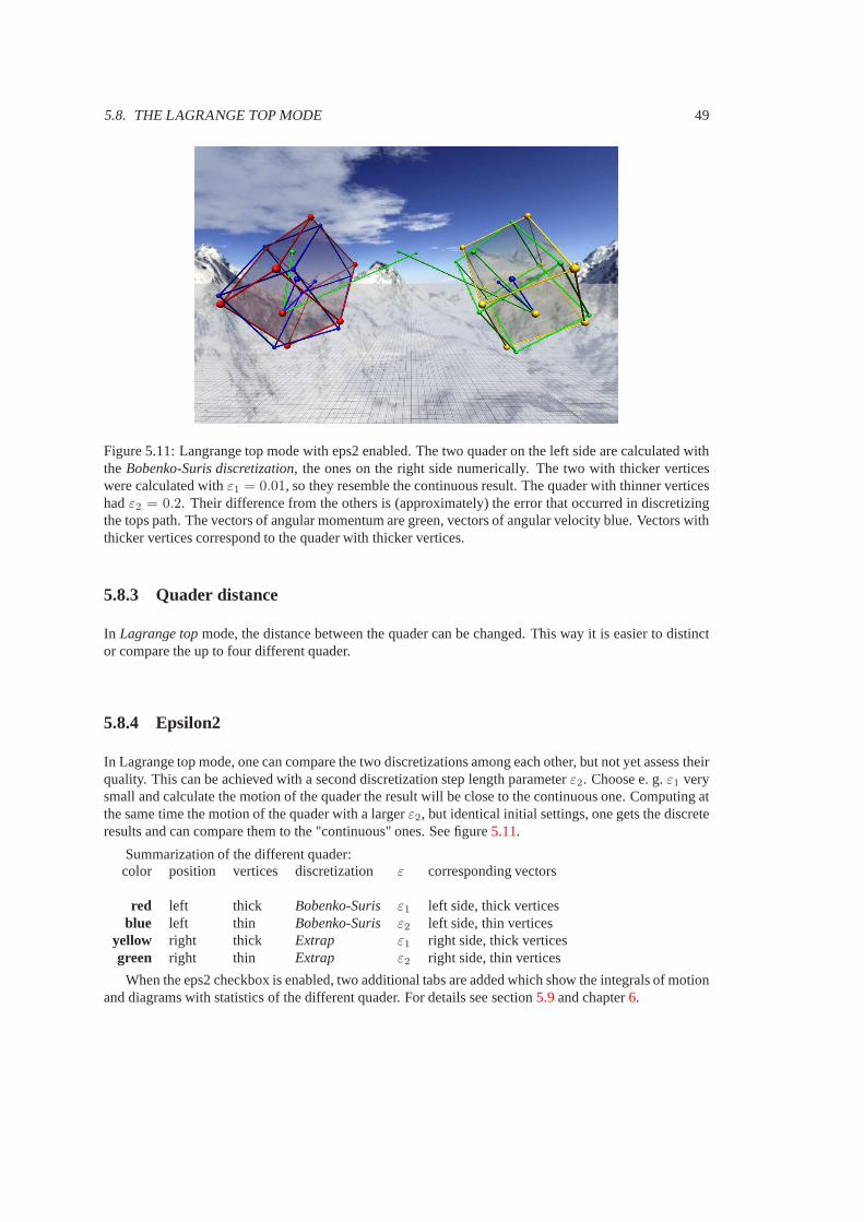
Figure 5.11: Langrange top mode with eps2 enabled. The two quader on the left side are calculated withthe Bobenko-Suris discretization, the ones on the right side numerically. The two with thickerverticeswere calculated withε1 = 0.01, so they resemble the continuous result. The quader with thinner verticeshadε2 = 0.2. Their difference from the others is (approximately) the error that occurred in discretizingthe tops path. The vectors of angular momentum are green, vectors of angular velocity blue. Vectors withthicker vertices correspond to the quader with thicker vertices.
5.8.3 Quader distance
In Lagrange topmode, the distance between the quader can be changed. This way it is easier to distinctor compare the up to four different quader.
5.8.4 Epsilon2
In Lagrange top mode, one can compare the two discretizations among each other, but not yet assess theirquality. This can be achieved with a second discretization step length parameterε2. Choose e. g.ε1 verysmall and calculate the motion of the quader the result will be close to the continuous one. Computing atthe same time the motion of the quader with a largerε2, but identical initial settings, one gets the discreteresults and can compare them to the "continuous" ones. See figure5.11.
Summarization of the different quader:color position vertices discretization ε corresponding vectors
red left thick Bobenko-Suris ε1 left side, thick verticesblue left thin Bobenko-Suris ε2 left side, thin vertices
yellow right thick Extrap ε1 right side, thick verticesgreen right thin Extrap ε2 right side, thin vertices
When the eps2 checkbox is enabled, two additional tabs are added which show the integrals of motionand diagrams with statistics of the different quader. For details see section5.9and chapter6.
50 CHAPTER 5. CALCULATION AND THE TOP VISUALIZATION
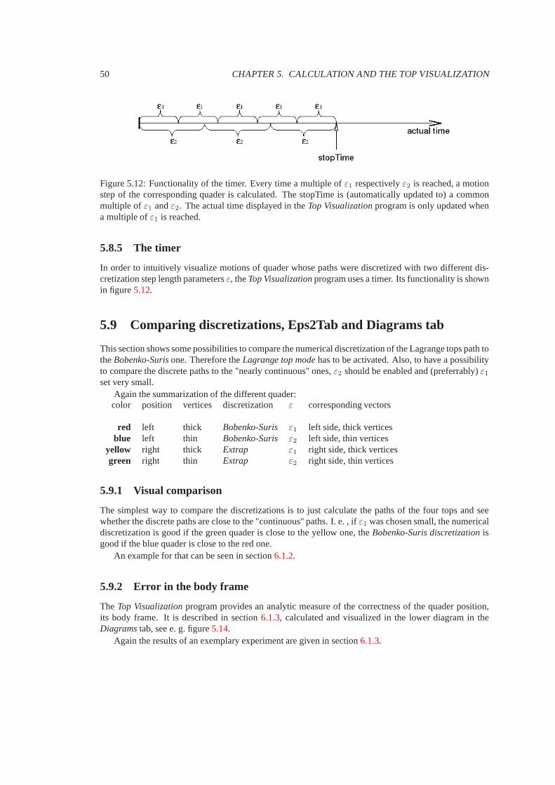
Figure 5.12: Functionality of the timer. Every time a multiple of ε1 respectivelyε2 is reached, a motionstep of the corresponding quader is calculated. The stopTime is (automatically updated to) a commonmultiple of ε1 andε2. The actual time displayed in theTop Visualizationprogram is only updated whena multiple ofε1 is reached.
5.8.5 The timer
In order to intuitively visualize motions of quader whose paths were discretized with two different dis-cretization step length parametersε, theTop Visualizationprogram uses a timer. Its functionality is shownin figure5.12.
5.9 Comparing discretizations, Eps2Tab and Diagrams tab
This section shows some possibilities to compare the numerical discretization of the Lagrange tops path totheBobenko-Surisone. Therefore theLagrange top modehas to be activated. Also, to have a possibilityto compare the discrete paths to the "nearly continuous" ones,ε2 should be enabled and (preferrably)ε1
set very small.Again the summarization of the different quader:color position vertices discretization ε corresponding vectors
red left thick Bobenko-Suris ε1 left side, thick verticesblue left thin Bobenko-Suris ε2 left side, thin vertices
yellow right thick Extrap ε1 right side, thick verticesgreen right thin Extrap ε2 right side, thin vertices
5.9.1 Visual comparison
The simplest way to compare the discretizations is to just calculate the paths of the four tops and seewhether the discrete paths are close to the "continuous" paths. I. e. , ifε1 was chosen small, the numericaldiscretization is good if the green quader is close to the yellow one, theBobenko-Suris discretizationisgood if the blue quader is close to the red one.
An example for that can be seen in section6.1.2.
5.9.2 Error in the body frame
The Top Visualizationprogram provides an analytic measure of the correctness of the quader position,its body frame. It is described in section6.1.3, calculated and visualized in the lower diagram in theDiagramstab, see e. g. figure5.14.
Again the results of an exemplary experiment are given in section 6.1.3.
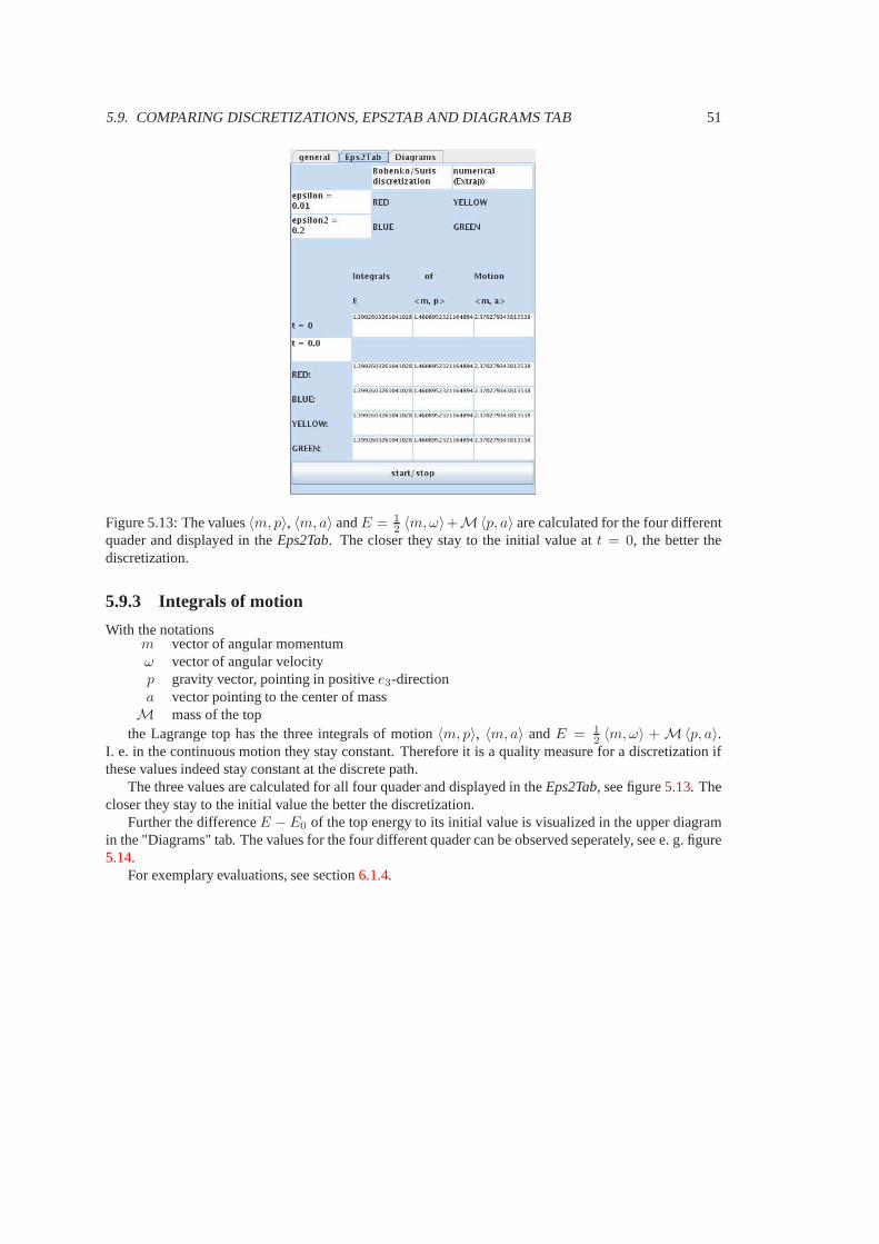
5.9. COMPARING DISCRETIZATIONS, EPS2TAB AND DIAGRAMS TAB 51
Figure 5.13: The values〈m, p〉, 〈m, a〉 andE = 12 〈m, ω〉+M〈p, a〉 are calculated for the four different
quader and displayed in theEps2Tab. The closer they stay to the initial value att = 0, the better thediscretization.
5.9.3 Integrals of motion
With the notationsm vector of angular momentumω vector of angular velocityp gravity vector, pointing in positivee3-directiona vector pointing to the center of mass
M mass of the topthe Lagrange top has the three integrals of motion〈m, p〉, 〈m, a〉 andE = 1
2 〈m, ω〉 + M〈p, a〉.I. e. in the continuous motion they stay constant. Thereforeit is a quality measure for a discretization ifthese values indeed stay constant at the discrete path.
The three values are calculated for all four quader and displayed in theEps2Tab, see figure5.13. Thecloser they stay to the initial value the better the discretization.
Further the differenceE − E0 of the top energy to its initial value is visualized in the upper diagramin the "Diagrams" tab. The values for the four different quader can be observed seperately, see e. g. figure5.14.
For exemplary evaluations, see section6.1.4.

52 CHAPTER 5. CALCULATION AND THE TOP VISUALIZATION
Figure 5.14: The upper diagrams shows the error in the energyof the different discretizations. The lowerone shows the measured error in the body frame. The errors canbe shown seperatelyby activating thecorresponding checkboxes. The errors in the lower diagram only make sense for the blue and the greenquader and ifε1 was chosen small.
Chapter 6
Results
6.1 Comparison of theBobenko-Suris discretization to the Extrapmethod
In this section theBobenko-Suris discretizationof the path of a Lagrange top is compared to a numericaldiscretization, i. e. theExtrapmethod of solving ordinary differential equations. Therefore the motionof the top was calculated with the two different discretization methods and with two differentε. Theinitial settings were chosen arbitrary. One can repeat the experiments in theTop Visualizationprogram.At startup the quader have the same settings used for the experiment in this section.
6.1.1 Settings
In the experiments there are four different quader. See figure 6.1for an example of the quader after theyalready moved for 300 time units.
They all had the same position, the same size, density, vector of angular momentum and gravity vectorat time zero.
For better distinction, they lie in two coordinate systems with shifted origin. The two quader on theleft side, the red and the blue one, had their motion calculated with theBobenko-Suris discretization, thetwo on the right side, yellow and green, numerically.
On each side there is one quader with thicker vertices and onewith thinner ones. The quader withthick vertices, red on the left side and yellow on the right side, had their motion calculated with theparameterε1. The quader with thin vertices with parameterε2.
The experiment took place in theLagrange top modewith a smallε1, so that the motions of the redand yellow quader, both with thick vertices, resemble the continuous motion.
The used numerical method isExtrap implemented in the package [TBb], see section4.1.1, withaccuracy parameters ofAtol = Rtol = 10−5 (chosen experimentally to balance calculation time andaccuracy) and the standard initial step size ofh = 0.1. This method showed a better performance thane. g. theRunge-Kuttamethod of solving ordinary differential equations.
The data used for the experiment is:ε1 0.01ε2 0.2
gravity 1quader coordinates (0.8, 0.8, 1)
vector of angular momentum (0.172, −1.862, 1.46)
53
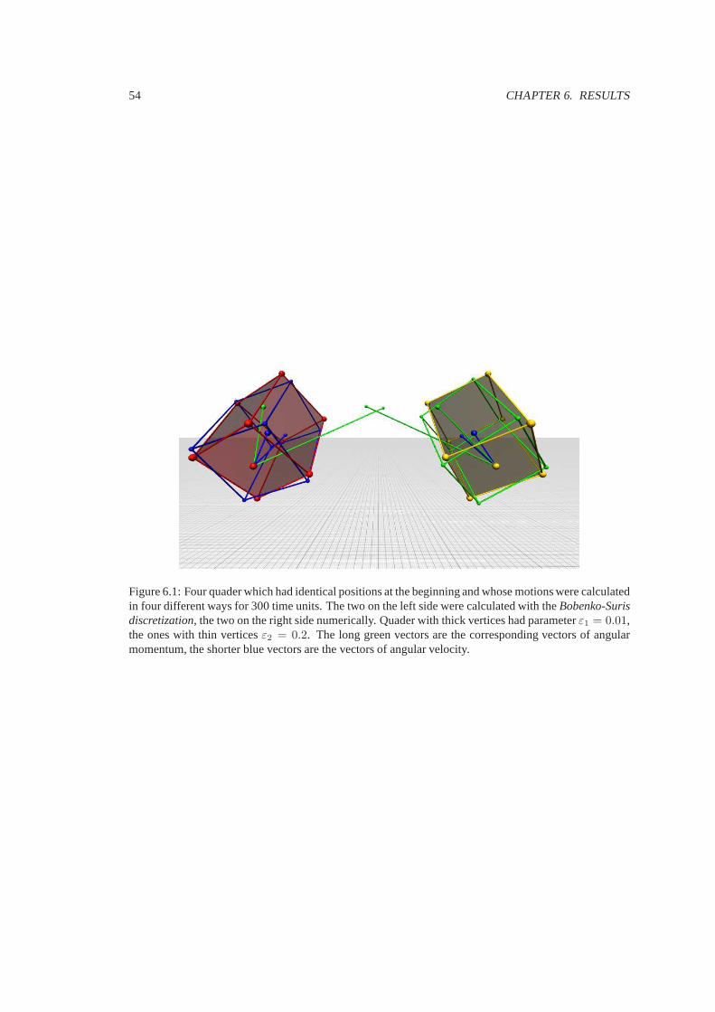
54 CHAPTER 6. RESULTS
Figure 6.1: Four quader which had identical positions at thebeginning and whose motions were calculatedin four different ways for 300 time units. The two on the left side were calculated with theBobenko-Surisdiscretization, the two on the right side numerically. Quader with thick vertices had parameterε1 = 0.01,the ones with thin verticesε2 = 0.2. The long green vectors are the corresponding vectors of angularmomentum, the shorter blue vectors are the vectors of angular velocity.
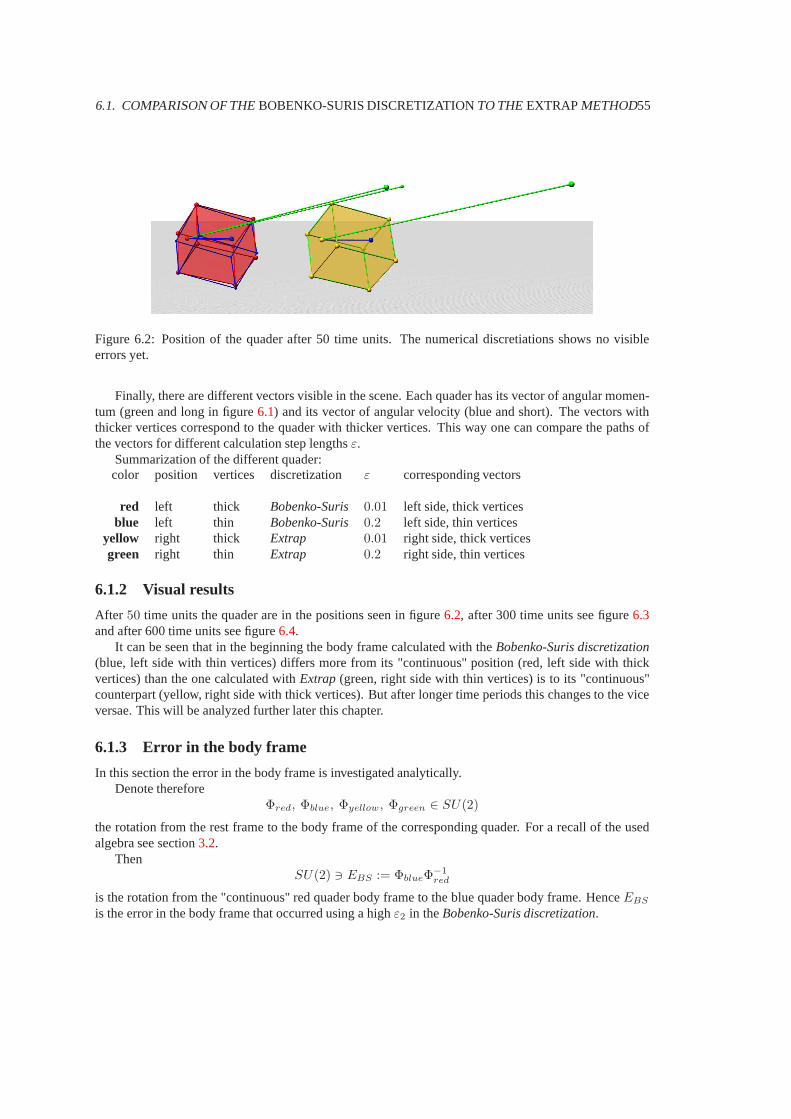
6.1. COMPARISON OF THEBOBENKO-SURIS DISCRETIZATIONTO THE EXTRAPMETHOD55
Figure 6.2: Position of the quader after 50 time units. The numerical discretiations shows no visibleerrors yet.
Finally, there are different vectors visible in the scene. Each quader has its vector of angular momen-tum (green and long in figure6.1) and its vector of angular velocity (blue and short). The vectors withthicker vertices correspond to the quader with thicker vertices. This way one can compare the paths ofthe vectors for different calculation step lengthsε.
Summarization of the different quader:color position vertices discretization ε corresponding vectors
red left thick Bobenko-Suris 0.01 left side, thick verticesblue left thin Bobenko-Suris 0.2 left side, thin vertices
yellow right thick Extrap 0.01 right side, thick verticesgreen right thin Extrap 0.2 right side, thin vertices
6.1.2 Visual results
After 50 time units the quader are in the positions seen in figure6.2, after 300 time units see figure6.3and after 600 time units see figure6.4.
It can be seen that in the beginning the body frame calculatedwith theBobenko-Suris discretization(blue, left side with thin vertices) differs more from its "continuous" position (red, left side with thickvertices) than the one calculated withExtrap (green, right side with thin vertices) is to its "continuous"counterpart (yellow, right side with thick vertices). But after longer time periods this changes to the viceversae. This will be analyzed further later this chapter.
6.1.3 Error in the body frame
In this section the error in the body frame is investigated analytically.Denote therefore
Φred, Φblue, Φyellow, Φgreen ∈ SU(2)
the rotation from the rest frame to the body frame of the corresponding quader. For a recall of the usedalgebra see section3.2.
ThenSU(2) ∋ EBS := ΦblueΦ
−1red
is the rotation from the "continuous" red quader body frame to the blue quader body frame. HenceEBS
is the error in the body frame that occurred using a highε2 in theBobenko-Suris discretization.
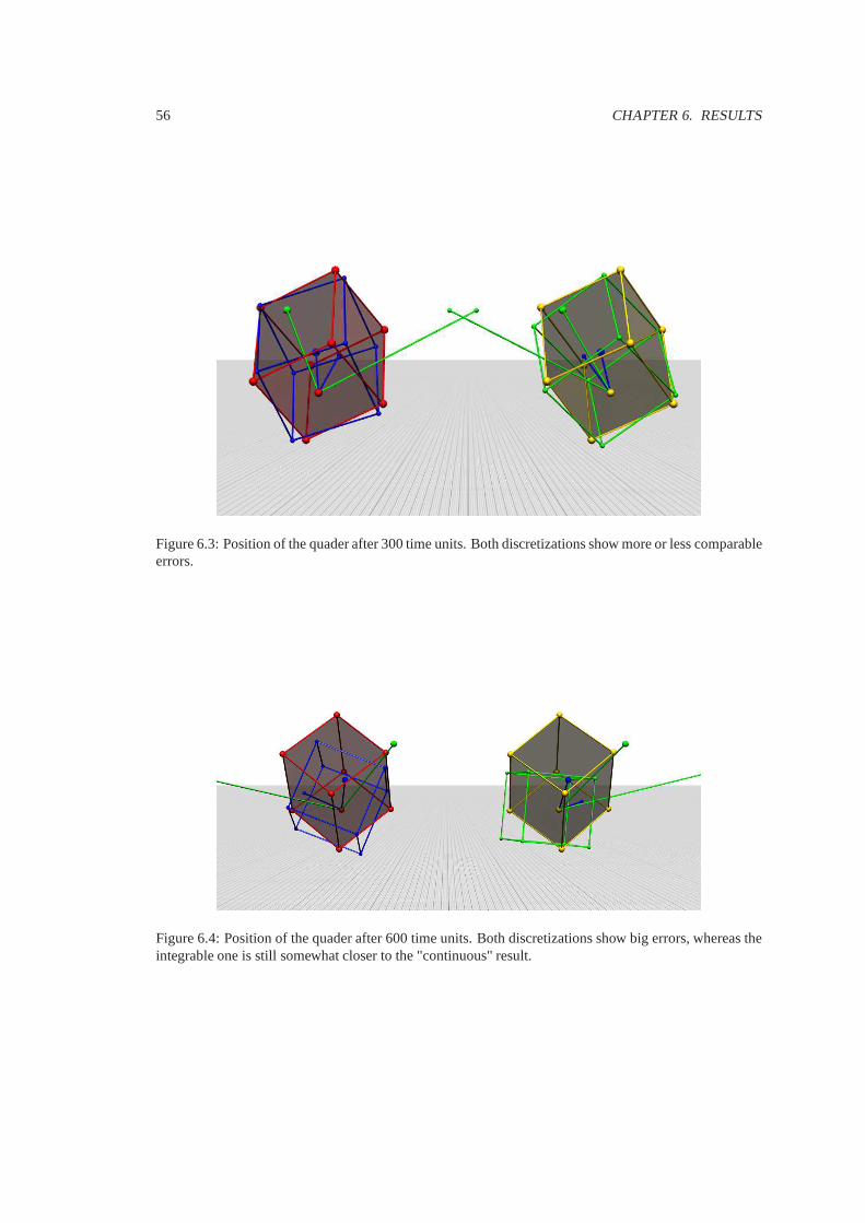
56 CHAPTER 6. RESULTS
Figure 6.3: Position of the quader after 300 time units. Bothdiscretizations show more or less comparableerrors.
Figure 6.4: Position of the quader after 600 time units. Bothdiscretizations show big errors, whereas theintegrable one is still somewhat closer to the "continuous"result.

6.1. COMPARISON OF THEBOBENKO-SURIS DISCRETIZATIONTO THE EXTRAPMETHOD57
Figure 6.5: L(E), the length of the geodesic from E to N, as measure of the error in the body frame E.
Similarly letSU(2) ∋ EExt := ΦgreenΦ−1
yellow
be the error in the body frame that occurred using a highε2 in theExtrapdiscretization.To make these error matrices comparable, consider the following observations. An arbitrary rotation
E ∈ SU(2) can be written as
E =
(a b−b a
)a, b ∈ C
=
(a1 + ia2 b1 + ib2
−b1 + ib2 a1 − ia2
)ai, bi ∈ R
with
det(E) = 1
⇔ a21 + a2
2 + b21 + b2
2 = 1.
ThereforeEBS andEExt correspond to vectors inS3. The identity matrix, which corresponds to "noerror in the body frame", hasa1 = 1 and a2 = b1 = b2 = 0, which is the north pole of the unit sphereS3. Hence the error in the body frame is the smaller the closer its corresponding vector inS3 lies to thenorth pole. See figure6.5.
As a measure of the errors in the rest frame one can use the length of the geodesic from an errormatrixE ∈ S3 to the north pole ofS3.
L : S3 7−→ R+
E −→ L(E) = length of geodesic fromE to N
Since the geodesics onS3 are great circles and the length of a segment betweenE andN is the includedangle, one gets
L(E) := ∡(E, N) = arccos〈E, N〉
‖E‖ · ‖N‖ = arccos(a1) ∈ [0, π].

58 CHAPTER 6. RESULTS
Figure 6.6: Errors in the body frame forε = 0.2 after 50 time units. The error in the numerical discretiza-tion is neglible compared to the one in the integrable discretization.
But since by theorem3.4 the error matrices inSU(2) are only unique up toΦ 7→ ±Φ and in theimplementation it cannot be determined, which one is obtained, in theTop Visualizationprogram‖a1‖ isused instead ofa1. Hence
L(E) := arccos(‖a1‖) ∈ [0,π
2]
is used.L(EBS) andL(EExt) are calculated and visualized in diagrams, see figures6.6, 6.7and6.8.In both discretizations there seems to be a fluctuation and a trend, though in theBobenko-Suris dis-
cretizationthe trend seems almost linear, whereas in the numerical one it is more or less quadratic.
6.1.4 Error in the integrals of motion
With the notationsm vector of angular momentumω vector of angular velocityp gravity vector, pointing in positivee3-directiona vector pointing to the center of mass
M mass of the topthe Lagrange top has the three integrals of motion〈m, p〉, 〈m, a〉 andE = 1
2 〈m, ω〉 + M〈p, a〉.In the experiment〈m, p〉 stays constant in both discretizations and for allε.The behaviour of〈m, a〉 for ε = 0.2 can be seen in figure6.9. The seen value is the actual〈m, a〉
minus the one att = 0. The integrable discretization yields as expected no errorsince it is an integral ofmotion of theBobenko-Suris discretization, see [BS00]. In the numerical discretization the error smallbut it is constantly increasing.
Another quality measure for the different discretizationsof the tops path is the error in the energy ofthe topE − E0, E0 being the energy att = 0. The error in theBobenko-Suris discretizationshows aperiodic behaviour proportional toε, see figure6.10.
For a comparison to the error in the energy in the numerical discretization see figure6.11. The errorin the numerical discretization increases fast after longer time periods, while the error in the integrable
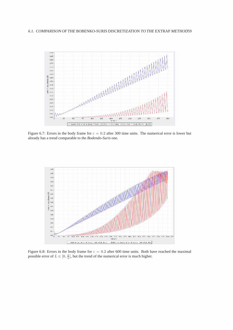
6.1. COMPARISON OF THEBOBENKO-SURIS DISCRETIZATIONTO THE EXTRAPMETHOD59
Figure 6.7: Errors in the body frame forε = 0.2 after 300 time units. The numerical error is lower butalready has a trend comparable to theBodendo-Surisone.
Figure 6.8: Errors in the body frame forε = 0.2 after 600 time units. Both have reached the maximalpossible error ofL ∈ [0, π
2 ], but the trend of the numerical error is much higher.
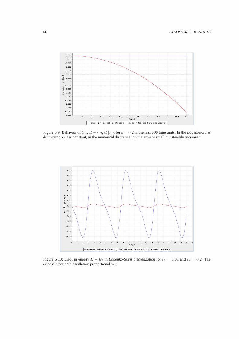
60 CHAPTER 6. RESULTS
Figure 6.9: Behavior of〈m, a〉 − 〈m, a〉 |t=0 for ε = 0.2 in the first 600 time units. In theBobenko-Surisdiscretizationit is constant, in the numerical discretization the error issmall but steadily increases.
Figure 6.10: Error in energyE − E0 in Bobenko-Suris discretizationfor ε1 = 0.01 andε2 = 0.2. Theerror is a periodic oszillation proportional toε.

6.2. COMPARISON OF THEBOBENKO-SURIS DISCRETIZATIONTO EXTRAPCOMPRISING EXECUTION TIME61
Figure 6.11: Error in energyE − E0 in both discretizations forε2 = 0.2. In the beginning the numericalerror is very small. Later it increases fast while the integrable error stays oscillating.
case keeps oscillating constantly.Reason for this oscillation is that this integrable discretization has the discrete integral of motion
Hε =1
2〈m, m〉 + 〈p, a〉 +
ε
2〈a × m, p〉 ,
see [BS00]. Thereby the used values are the coordinates wrt the scaledcoordinate system, see section4.2.1. The first two terms inHε are the energy of the top in these coordinates. The valueHε indeed staysconstant in the experiment which implies that the error in the energy in theBobenko-Suris discretizationis the additional termε
2 〈a × m, p〉.
6.1.5 Further Observations
In figure6.12the error in the energy of the top is opposed to the error in thebody frame in theBobenko-Suris discretizationfor ε = 0.2. One can observe a correlation between the oscillating error in energycaused by the termε2 〈a × m, p〉 and the oscillating part of the error in the body frame.
Moreover, the termε2 〈a × m, p〉 plays a central role for the quality of the integrable discretization.
E. g. using settings that increase this term, like a vector ofangular momentumm that is longer or moreperpendicular to the center of massa, or a higher gravity constantg and hence a longer gravity vectorp, the exactness of the discrete motion decreases. See figures6.13and6.14for the results of a motionwith initial settings as above except of a gravity constant of g = 10 and a vector of angular momentumm = (5, 0, 0).
As expected the results of the integrable discretization are very bad.
6.2 Comparison of theBobenko-Suris discretization to Extrap com-prising execution time
The first experiment is in so far unfair, that the numerical discretization is a multi-step method and workseffectively with a (variable but) smaller discretization step length parameter than the integrable discretiza-

62 CHAPTER 6. RESULTS
Figure 6.12: Error in energyE−E0 opposed to the error in the body frameL(EBS) in theBobenko-Surisdiscretizationfor ε = 0.2. One can observe a correlation between the (oscillating) error in the energy andthe oscillating part of the error in the body frame.
Figure 6.13: Visual result of an experiment with a high errorterm ε2 〈a × m, p〉 aftert = 20 time units.
The position of the quader calculated with the integrable discretization is already very wrong after thatshort time period.

6.2. COMPARISON OF THEBOBENKO-SURIS DISCRETIZATIONTO EXTRAPCOMPRISING EXECUTION TIME63
Figure 6.14: Error in the energy in an experiment with a high error term ε2 〈a × m, p〉 after t = 20 time
units. The oscillating error in the energy of the integrablediscretization is of very high magnitude.
tion. Further the numerical method needs more execution time.
When asking the question, which discretization is more suitable for practical purposes, one mightwant to compare their performance for a given amount of computational capacity. This is done in anexample in this section.
Unfortunately this was only possible with modified source code of theTop Visualizationprogram andcan therefore not be repeated like the first experiment.
6.2.1 Settings
The initial position of the quader, vectors of angular velocity and momentum and gravity vector are thesame as in the first experiment.
In order to compare the discretizations for a fixed given execution time, only the discretization steplength parameter and the error tolerancesAtol andRtol, see section4.1.1, are changed. I. e. the usedvalues are:

64 CHAPTER 6. RESULTS
ε1 = 0.01 the parameter for the "continuous" motion, to assess the discreteones.
ε2 = 5 the interval length, for which the discretizations will be assigned afixed amount of execution time to compute a best possible result.The quaders path is continuously calculated after every 5 time unitsteps, so that it can be determined up to arbitrary time points5n, n ∈N, and the results can be compared after every 5 time units.
m = 166 the number of intervals[5n, 5(n + 1)], n ∈ N, is seperated into fortheBobenko-Surisdiscretization. This yields an effective discretiza-tion step length parameter of 0.03.
Atol = Rtol = 2 · 10−8 the error tolerances for theExtrapmethod, see section4.1.1.
h = 1.5 the initial step size at the beginning of each interval[5n, 5(n + 1)],n ∈ N. Changing this step size within this order of magnitudeshowed practically no change, since it is quickly adjusted by theEx-trap method and since initially too highh are rejected without muchloss of calculation time.
These values were determined experimentally to satisfy thefollowing conditions:
1. Both discretization methods use the same amount of execution time. With these settings theyneeded an average of 0.8 milliseconds to calculate the next quader position after further 5 timeunits. The calculations were done in JavaTM on a Linux system with an IntelR© CoreTM 2 Duo CPUwith 2 × 2.00GHz.
2. ε2 = 5 andAtol = Rtol = 2 · 10−8 were chosen in such a way, that theExtrapmethod could useits property of step size control effectively. For the interval [5n, 5(n + 1)], n ∈ N, an average of 7steps are calculated.
3. The for theBobenko-Surisdiscretization effectively used discretization step length parameter 0.03is still comparable to the parameter 0.01 used for the "continuous" result.
These settings yielded the following results.
6.2.2 Visual results
The visual results of the experiment can be seen in figures6.15, 6.16, 6.17and6.18.It can be observed that in the beginning the numerical discretization yields better results, but its
transported errors accumulate in time and let it yield weaker results after longer time periods.
6.2.3 Error in the body frame
The errors in the body frame, see section6.1.3, can be seen in figures6.19, 6.20and6.21.
6.2.4 Error in the energy
The errors in the energy of the quader can be seen in figures6.22and6.23.

6.2. COMPARISON OF THEBOBENKO-SURIS DISCRETIZATIONTO EXTRAPCOMPRISING EXECUTION TIME65
Figure 6.15: Position of the four quader aftert = 200 time units in the experiment comprising executiontime. There are almost no errors recognizable.
Figure 6.16: Position of the four quader aftert = 600 time units in the experiment comprising executiontime. Both discretizations start to show errors, whereas theBobenko-Surisdiscretization has a little highererror in the quader position.

66 CHAPTER 6. RESULTS
Figure 6.17: Position of the four quader aftert = 1000 time units in the experiment comprising executiontime. The errors in the numerical discretization increase faster.
Figure 6.18: Position of the four quader aftert = 3200 time units in the experiment comprising executiontime. The errors in the integrable discretization are stillsomewhat acceptable, while the errors in thenumerical one have gotten very big.

6.2. COMPARISON OF THEBOBENKO-SURIS DISCRETIZATIONTO EXTRAPCOMPRISING EXECUTION TIME67
Figure 6.19: Errors in the body frame aftert = 400 time units in the experiment comprising executiontime. The error in theBobenko-Surisdiscretization is higher. The numerical error is neglible in thebeginning and low after 200 to 400 time units.
Figure 6.20: Errors in the body frame aftert = 1000 time units in the experiment comprising executiontime. After about 900 time units the numerical error equals the integrable one more or less, but it increasesfaster.

68 CHAPTER 6. RESULTS
Figure 6.21: Errors in the body frame aftert = 3200 time units in the experiment comprising executiontime. The integrable discretization still yields a relatively small error, whereas the numerical error alreadyreached the maximally possible value ofL ∈ [0, π
2 ].
Figure 6.22: Errors in the energy aftert = 1000 time units in the experiment comprising execution time.The error in the integrable discretization is the oscillation due to the termε
2 〈a × m, p〉, see section6.1.4.The error in the numerical discretization is small but steadily increasing.
Figure 6.23: Errors in the energy aftert = 3200 time units in the experiment comprising execution time.The numerical error reaches the magnitude of the integrableerror, and keeps increasing.

6.3. COMPARISON OF THEBOBENKO-SURIS DISCRETIZATIONTO THE RUNGE-KUTTAMETHOD69
Figure 6.24: Errors in the energy aftert = 30 time units in the experiment with comparable step sizes.The error in theRunge-Kuttamethod is small for a short time period, but increases strongly later on.
It can be observed that the error in the integrable discretization is the oscillation due to the termε2 〈a × m, p〉, see section6.1.4, and that the numerical error increases steadily. The latter is due to thefact that the local errors are transported and add up to an increasing global error.
6.3 Comparison of theBobenko-Suris discretization to the Runge-Kutta method
The above experiments all used different step sizes in the different discretizations. For further clarificationof theBobenko-Suris discretizations properties now follow the results of an experiment, where the numberof evaluations of the equations of motion is equal for the twodiscretization.
Let thereforeε2 be the (constant) step size used in theclassical 4th order Runge-Kuttamethod (TheRunge-Kutta method). Since this is a 4 step method, i. e. the equation of motion is evaluated 4 times fordoing one step, theBobenko-Suris discretizationworks with an effective step size ofε2/4, since it doesso only once. The other settings are the same as in the former experiments.
Then for the experiments results withε2 = 0.2 see figures6.24and6.25.It can be observed that theRunge-Kuttamethod yields good results for a short time period. Later on,
when the transported errors accumulate and amplify themselves, the results get very bad.The same happens, just after a different amount of time, for other discretization step length parameter
ε2 ∈ [0.1, 0.6]. For largerε2 the results diverge very soon.
6.4 Conclusions
TheBobenko-Suris discretizationshows both, advantages and disadvantages, compared to the numericaldiscretization.

70 CHAPTER 6. RESULTS
Figure 6.25: Errors in the frame aftert = 30 time units in the experiment with comparable step sizes.Here too, the error in theRunge-Kuttamethod is small in the beginning, but grows quickly.
Mentionable disadvantages are the systematically occurring error in the energy of the top and theresulting error in the body frame already after relatively short time periods. The path of the top is adifferent one form the real motion. Further there is no step size control, which could make it moreaccurate in regions of the equations of motion with high derivatives.
Advantages are the oscillation of the error in the energy, itdoes not increase continuously like innumerical discretizations which makes it more suitable forlong time period calculations. Further thereis still a large potential in improving this discretization, e. g making it a higher order approximation oradding a step size control.
6.5 Prospects
The Top Visualizationprogram was not designed for an optimized calculation of thetops paths. Theexperiment comprising execution time was very rough and done only for a special initial setting. Asource code optimized for execution time and an applicationto a wider range of initial settings wouldsurely clarify the properties of theBobenko-Suris discretizationmore than was done in this thesis.
Further theBobenko-Suris discretizationsitself could be improved. As derived in [BS00] it is basedon a first order discretization of the frame of an isotropic elastic rod with equidistant step sizes. It couldbe extended to higher order terms, and possibly even includestep size control and an automatic orderselection.

Appendix A
Abstract in german -Zusammenfassung auf Deutsch
Der Inhalt dieser Diplomarbeit ist ein Vergleich von Diskretisierungen der Bewegungen des Lagrange-Kreisels. Die in [BS00] entwickelte integrable Diskretisierung wird mit numerischen Lösungen vergli-chen, um deren Vor- oder Nachteile gegenüberzustellen. Dies geschieht mittels Implementation der ver-schiedenen Diskretisierungen in einemJavaTM ProgrammTop Visualization, welches Teil dieser Di-plomarbeit ist.
Dazu werden in Kapitel2 die Grundlagen über Kreisel im Allgemeinen und den Lagrange-Kreisel imspeziellen wiederholt. In Beispielen werden diese auf den Fall eines Quader angewandt, welche imTopVisualizationProgramm für die Berechnung und Visualisierung genutzt werden. Kapitel3 befasst sichmit der kontinuierlichen Dynamik des Kreisels, Kapitel4 mit deren Diskretisierung.
DasTop VisualizationProgramm wird in Kapitel5 beschrieben. Es liegt der Diplomarbeit auf ei-ner CD bei, kann aber auch im Internet unterhttp://www.math.tu-berlin.de/˜bodackheruntergeladen oderdirekt als Webstart-Applikation unterhttp://www.math.tu-berlin.de/geometrie/ps/software.shtmlgestar-tet werden. Damit können die Eigenschaften des Lagrange-Kreisels selbstständig studiert und die Dis-kretisierungen selbst verglichen werden. Die Ergebnisse eines beispielhaften Vergleichs sind in Kapitel6 gegeben. Desweiteren enthält Kapilel6 die Resultate zweier zusätzlicher Experimente, die weitereEinblicke in die Eigenschaften der integrablen Diskretisierung geben. Es stellt sich heraus, dass dieseDiskretisierung für Berechnungen des Kreiselpfades über kurze Zeitperioden ungeeignet ist, für längereIntervalle aber klar dominiert.
Weiterhin bietet dasTop VisualizationProgramm eine Visualisierung der Bewegung von beliebigenQuadern und der intergrablen Spezialfälle des Kowalewski-und des Goryachev-Chaplygin-Kreisels. Einekurze Beschreibung dieser Fälle findet man in Kapitel5. Das Programm zeigt auch die Drehmoment-und Winkelgeschwindigkeitsvektoren der Kreisel, ihre Hauptträgheitsachsen und (falls diese existieren)ihre zugehörigen elastischen Stäbe. Desweiteren wird die typische Bewegung des Lagrange-Kreisels ausPräzession und Nutation mit dem sogenanntenapex tracevisualisiert.
71

72 APPENDIX A. ABSTRACT IN GERMAN - ZUSAMMENFASSUNG AUF DEUTSCH

Bibliography
[Arn] V. I. Arnold, Mathematical methods of classical mechanics, Springer-Verlag, Berlin, 1978.
[BBEIM] E. D. Belokolos, A. I. Bobenko, V. Z. Enol’Skii, A. R.Its, V. B. Matveev,Algebro-GeometricApproach to Nonlinear Integrable Equations, Springer-Verlag, Berlin, 1994.
[BS00] A. I. Bobenko and Yu- B. Suris,A Discrete Time Lagrange Top and Discrete Elastic Curves,Amer. Math. Soc. Transl. (2) Vol. 201, 2000.
[B97] A. I. Bobenko,Mathematik des Kreisels, lecture notes
[B06] A. I. Bobenko, Differtialgeometrie von Kurven und Flächen,http://www.math.tu-berlin.de/ bobenko/skripte.html
[HNW] E. Hairer, S. P. Norsett and G. Wanner,Solving ordinary differential equations I. Nonstiffproblems., 2nd edition, Springer series in computational mathematics, Springer-Verlag, 1993.
[MTJ] Matrix Toolkits for Java (MTJ), http://ressim.berlios.de
[TBa] TU-Berlin, JReality, a Java 3D Viewer for Mathematics, http://www.jreality.de.
[TBb] TU-Berlin, Java Tools for Experimental Mathematics, http://www.jtem.de.
73