d experimental nuclear and particle physics
TRANSCRIPT
CZECH TECHNICAL UNIVERSITY
IN PRAGUE
FACULTY OF NUCLEAR SCIENCES AND
PHYSICAL ENGINEERING
Department of Physics
Experimental Nuclear and Particle Physics
Master’s thesis
Study of jet shape observables in Au+Au
collisions in the STAR experiment
Author: Bc. Veronika ProzorovaSupervisor: RNDr. Jana Bielcıkova, Ph.D.
Prague, 2020


CESKE VYSOKE UCENI TECHNICKE
V PRAZE
FAKULTA JADERNA A FYZIKALNE
INZENYRSKA
Katedra fyziky
Experimentalnı jaderna a casticova fyzika
Diplomova prace
Studium tvaru jetu v Au+Au srazkach v
experimentu STAR
Vypracovala: Bc. Veronika Prozorova
Skolitel: RNDr. Jana Bielcıkova, Ph.D.Praha, 2020


Prohlasenı
Prohlasuji, ze jsem svou diplomovou praci vypracovala samostatne a pouzila jsempouze podklady (literaturu, projekty, SW atd.) uvedene v prilozenem seznamu.
Nemam zavazny duvod proti pouzitı tohoto skolnıho dıla ve smyslu §60 Zakonac. 121/2000 Sb., o pravu autorskem, o pravech souvisejıcıch s pravem autorskym ao zmene nekterych zakonu (autorsky zakon).
V Praze dne .........................................................Bc. Veronika Prozorova


Nazev prace: Studium tvaru jetu v Au+Au srazkach v experimentu STAR
Autor: Bc. Veronika Prozorova
Obor: Experimentalnı jaderna a casticova fyzika
Druh prace: Diplomova prace
Vedoucı prace: RNDr. Jana Bielcıkova, Ph.D.
Ustav jaderne fyziky AV CR, v.v.i.
Abstrakt: Jadro-jaderne srazky pri energiıch dosazitelnych na urychlovaciRHIC v BNL v USA jsou idealnım prostredım ke studiu jaderne hmoty, existujıcı vextremnıch podmınkach vysokych teplot a hustot energiı. Jednou z nejdulezitejsıchsond teto jaderne hmoty je studium produkce jetu. V teto diplomove praci je jetovyalgoritmus anti-kT aplikovan na experimentalnı data z Au+Au srazek zmerena ex-perimentem STAR pri energii 200 GeV v tezist’ovem systemu na nukleon-nukleonovypar. Vybrane pozorovatelne popisujıcı tvar nabitych jetu jsou extrahovany pro ruznecentrality srazky a hodnoty prıcne hybnosti nabitych jetu. Take je proveden odpocetprumerneho pozadı pro tyto pozorovatelne.
Klıcova slova: jet, tvary jetu, RHIC, STAR, kvarkovo-gluonove plazma


Title: Study of jet shape observables in Au+Au collisionsin the STAR experiment
Author: Bc. Veronika Prozorova
Specialization: Experimental Nuclear and Particle Physics
Sort of project: Master’s thesis
Supervisor: RNDr. Jana Bielcıkova, Ph.D.
Ustav jaderne fyziky AV CR, v.v.i.
Abstract: The nucleus-nucleus collisions at energies attainable at the acceleratorRHIC in BNL in the US are an ideal environment to study nuclear matter existingin the conditions of extremely high temperature and density. One of the mostimportant probes is to study production of jets. In this master’s thesis the anti-kT jetfinding algorithm is applied to the experimental data from Au+Au collisions at thecenter of mass energy of 200 GeV per nucleon-nucleon pair in the STAR experiment.The chosen observables describing the shape of charged jets are extracted at thedetector level for different collision centralities and the transverse momentum of thecharged jets and are corrected for the average background.
Key words: jet, jet shapes, RHIC, STAR, quark-gluon plasma


Acknowledgement
I would like to express my sincere gratitude to my supervisor RNDr. JanaBielcıkova, Ph.D. for guiding this thesis, her willingness, patience, precious advicesand language corrections.
Additionally, I would like to thank Oleg Tsai, Akio Ogawa and David Ka-pukchyan from Brookhaven National Laboratory for giving me an opportunity tohelp with the Forward Calorimeter System Upgrade. The experience I got duringone month of working with these people is invaluable.
I am also thankful to my dear husband, my parents and friends for their supportduring all my research.
Bc. Veronika Prozorova

Contents
Preface 1
1 Heavy-ion collisions 3
1.1 Phase diagram of QCD matter . . . . . . . . . . . . . . . . . . . . . 3
1.2 Space-time evolution of a nucleus-nucleus collisions . . . . . . . . . . 4
1.3 Centrality of the collision . . . . . . . . . . . . . . . . . . . . . . . . 7
1.3.1 Centrality types . . . . . . . . . . . . . . . . . . . . . . . . . 7
1.3.2 Determination of centrality . . . . . . . . . . . . . . . . . . . 7
1.4 Glauber model of nucleus-nucleus collisions . . . . . . . . . . . . . . 9
1.5 Hard probes of the QCD medium . . . . . . . . . . . . . . . . . . . . 9
1.5.1 Jets . . . . . . . . . . . . . . . . . . . . . . . . . . . . . . . . 10
1.5.2 Heavy flavor . . . . . . . . . . . . . . . . . . . . . . . . . . . 10
1.6 Nuclear Modification factor . . . . . . . . . . . . . . . . . . . . . . . 12
2 Jets 17
2.1 Requirements for jet reconstructing algorithms . . . . . . . . . . . . 17
2.2 Sequential-clustering jet algorithms . . . . . . . . . . . . . . . . . . . 18
2.2.1 kT jet algorithm . . . . . . . . . . . . . . . . . . . . . . . . . 18
2.2.2 Anti-kT jet algorithm . . . . . . . . . . . . . . . . . . . . . . 19
2.3 Area related properties . . . . . . . . . . . . . . . . . . . . . . . . . . 20
2.4 FastJet . . . . . . . . . . . . . . . . . . . . . . . . . . . . . . . . . . 21
2.5 Constituent pile-up subtraction for jets . . . . . . . . . . . . . . . . . 22
2.6 Unfolding techniques . . . . . . . . . . . . . . . . . . . . . . . . . . . 24
2.6.1 Bayesian unfolding . . . . . . . . . . . . . . . . . . . . . . . . 24
2.6.2 Singular Value Decomposition . . . . . . . . . . . . . . . . . . 25
3 RHIC and STAR 27
3.1 RHIC . . . . . . . . . . . . . . . . . . . . . . . . . . . . . . . . . . . 27
3.2 STAR . . . . . . . . . . . . . . . . . . . . . . . . . . . . . . . . . . . 28
3.2.1 Time Projection Chamber . . . . . . . . . . . . . . . . . . . . 29
3.2.2 Barrel Electro-Magnetic Calorimeter . . . . . . . . . . . . . . 30
3.2.3 Endcap Electro-Magnetic Calorimeter . . . . . . . . . . . . . 32
3.2.4 Beam-Beam Counter . . . . . . . . . . . . . . . . . . . . . . . 32
3.2.5 Vertex Position Detector . . . . . . . . . . . . . . . . . . . . . 33
3.2.6 Zero-Degree Calorimeter . . . . . . . . . . . . . . . . . . . . . 33
3.2.7 Time Of Flight . . . . . . . . . . . . . . . . . . . . . . . . . . 35
3.2.8 Heavy Flavor Tracker . . . . . . . . . . . . . . . . . . . . . . 36
i
4 Contribution to the Forward Calorimeter System Upgrade 394.1 Forward Calorimeter System . . . . . . . . . . . . . . . . . . . . . . 394.2 HCal scintillating tiles . . . . . . . . . . . . . . . . . . . . . . . . . . 404.3 Calibration data for SiPMs in ECal . . . . . . . . . . . . . . . . . . . 414.4 Optimal operating voltage for SiPMs in FCS . . . . . . . . . . . . . 44
5 Data analysis 475.1 Jet shapes . . . . . . . . . . . . . . . . . . . . . . . . . . . . . . . . . 475.2 Dataset . . . . . . . . . . . . . . . . . . . . . . . . . . . . . . . . . . 485.3 Jet analysis . . . . . . . . . . . . . . . . . . . . . . . . . . . . . . . . 505.4 Angularity . . . . . . . . . . . . . . . . . . . . . . . . . . . . . . . . . 535.5 Momentum dispersion . . . . . . . . . . . . . . . . . . . . . . . . . . 57
6 Summary 61
APPENDICES 62
A Basic kinematic observables 63A.1 Transverse momentum . . . . . . . . . . . . . . . . . . . . . . . . . . 63A.2 Rapidity and pseudorapidity . . . . . . . . . . . . . . . . . . . . . . . 63A.3 Center-of-mass energy . . . . . . . . . . . . . . . . . . . . . . . . . . 64
B Bad run list 65
C Results 67
ii

List of Figures
1.1 A phase diagram of nuclear matter [1]. . . . . . . . . . . . . . . . . . 3
1.2 A space-time view of a central collision of two heavy nuclei (A+A)in the Landau picture. a) Two nuclei approaching each other withrelativistic velocities and zero impact parameter in the CMS frame.b) The slowing down of the nuclei with further interaction and par-ticle production. c) The light-cone representation of the high-energyhadron collision in the Landau picture. The shaded area is the parti-cle production area. . . . . . . . . . . . . . . . . . . . . . . . . . . . 4
1.3 A space-time evolution of the relativistic heavy-ion collision [2]. . . . 5
1.4 A space-time view of a central collision of two heavy nuclei (A+A) inthe Bjorken model. a) The central collision of two nuclei. b) Passageof the nuclei through each other. c) The light-cone representation ofthe high-energy nucleus-nucleus collision. The shaded area is the areaof forming the highly excited matter. . . . . . . . . . . . . . . . . . . 6
1.5 A schematic view of central, peripheral and ultra-peripheral collisions. 7
1.6 The measured charged particle multiplicity in Au+Au collisions at√sNN = 200
GeV by the STAR experiment together with corresponding values ofthe impact parameter b, number of participants Npart in the collisionsand fraction of geometrical cross-section σ/σtot [3]. . . . . . . . . . . 8
1.7 Geometry of a collision between nucleus A and nucleus B. with trans-verse (a) and longitudinal (b) views [4]. . . . . . . . . . . . . . . . . 9
1.8 A schematic view of jet created in a heavy-ion collision [5]. . . . . . 10
1.9 Quark masses in the QCD vacuum and the Higgs vacuum [6]. . . . . 11
1.10 Nuclear modification factor RAA of charged particles as a function ofpT in Pb+Pb collisions at
√sNN = 5.02 TeV compared to the results
at√sNN = 2.76 TeV from CMS, ALICE and ATLAS. Centrality
ranges: 0-5% (left), 50-70% (right). The systematic uncertainty ofthe 5.02 TeV CMS points is represented by yellow boxes. The blueand gray boxes represent the TAA and pp luminosity uncertainties,respectively. [7]. . . . . . . . . . . . . . . . . . . . . . . . . . . . . . . 12
1.11 Upper panel: Nuclear modification factor for D0 mesons in centralAu+Au collisions at
√sNN = 200 GeV at STAR compared to the
ALICE results at√sNN = 2.76 TeV. Bottom panel: Measurements of
charged pions from STAR and charged hadrons from ALICE [8]. . . 13
iii

1.12 Nuclear modification factor RAA as a function of jet pT for jets with|y| < 2.8 in different centrality intervals. Right: 10-20%, 30-40%,50-60%, 70-80%. Left: 0-10%, 20-30%, 40-50%, 60-70%. The pT
of constituents is > 10 GeV/c. pT of the tracks > 10 GeV/c. Thestatistical uncertainties and the bin-wise correlated systematic un-certainties are represented by the error-bars and the shaded boxesaround the data points, respectively. Fractional 〈TAA〉 and p+p lu-minosity uncertainties are shown as colored and grey shaded boxes,respectively, at RAA = 1 [9]. . . . . . . . . . . . . . . . . . . . . . . . 14
1.13 The RAA for jets as a function of pjetT for various resolution parametersand centrality classes [10]. . . . . . . . . . . . . . . . . . . . . . . . 14
1.14 Jet RAA at√sNN = 5.02 TeV for R = 0.2 with |ηjet| < 0.5 (left) and
R = 0.4 with |ηjet| < 0.7 (right) [11]. . . . . . . . . . . . . . . . . . . 15
1.15 Charged jet RCP with pleadT > 5 GeV for R = 0.2 - 0.4 [12]. . . . . . 15
2.1 An example of infrared sensitivity in cone jet clustering. Seed parti-cles are shown as arrows with the length proportional to energy [13]. 17
2.2 A sample parton-level event generated with HERWIG Monte-Carlogenerator of p+p collision clustered with kT (left) and anti-kT (right)algorithms [14]. . . . . . . . . . . . . . . . . . . . . . . . . . . . . . . 20
2.3 Distribution of areas in di-jet events at the LHC for various jet findingalgorithms. The events were generated by PYTHIA 6.4. (a) passivearea at parton level, (b) active area at hadron level including UE andpile-up [14]. . . . . . . . . . . . . . . . . . . . . . . . . . . . . . . . . 21
2.4 The running times of the kT jet-finder and FastJet implementationsof the kT clustering algorithm versus the number of initial particles [15]. 22
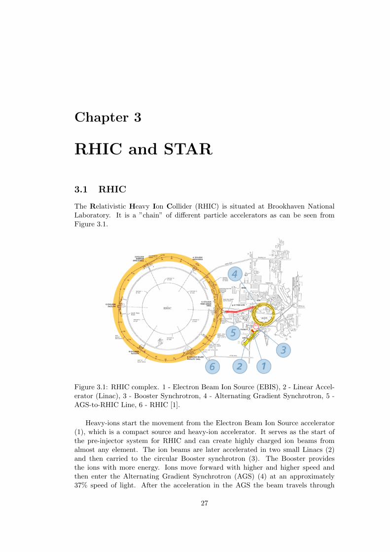
3.1 RHIC complex. 1 - Electron Beam Ion Source (EBIS), 2 - LinearAccelerator (Linac), 3 - Booster Synchrotron, 4 - Alternating GradientSynchrotron, 5 - AGS-to-RHIC Line, 6 - RHIC [1]. . . . . . . . . . . 27
3.2 A 3D model of the STAR detector system [16]. . . . . . . . . . . . . 28
3.3 The layout of the STAR Time Projection Chamber [17]. . . . . . . . 29
3.4 The ionization energy loss measured in 200 GeV Au+Au collisions atRHIC [18]. . . . . . . . . . . . . . . . . . . . . . . . . . . . . . . . . . 30
3.5 Cross sectional views of the STAR detector. The Barrel EMC covers|η| ≤ 1. The BEMC modules slide in from the ends on rails whichare held by aluminum hangers attached to the magnet iron betweenthe magnet coils [19]. . . . . . . . . . . . . . . . . . . . . . . . . . . . 31
3.6 A side view of the STAR BEMC module. The image shows the lo-cation of the two layers of shower maximum detector at a depth ofapproximately 5 radiation length X0 from the front face at η = 0 [19]. 31
3.7 Endcap Electro-Magnetic Calorimeter [16]. . . . . . . . . . . . . . . 32
3.8 The schematic view of the BBC position. The blue and yellow arrowsrepresent the differently polarized proton beams. . . . . . . . . . . . 33
3.9 A schematic view of the Beam-Beam Counter [16]. . . . . . . . . . . 33
3.10 A schematic side view of the Vertex Position Detector [20]. . . . . . 34
3.11 RHIC Zero-Degree Calorimeter [16]. . . . . . . . . . . . . . . . . . . 34
3.12 The TOF system [16]. . . . . . . . . . . . . . . . . . . . . . . . . . . 35
iv

3.13 The momentum dependence of the particle mass resolution for a100 ps time resolution for pions, kaons, protons and deuterons [21]. . 36
3.14 TOF particle identification from 1/β measured in 200 GeV Au+Aucollisions at RHIC [18]. . . . . . . . . . . . . . . . . . . . . . . . . . . 36
3.15 A schematic view of the Heavy Flavor Tracker inside the STAR de-tector [16]. . . . . . . . . . . . . . . . . . . . . . . . . . . . . . . . . . 37
3.16 The Heavy Flavor Tracker parts. PXL - Pixel Detector, IST - Inter-mediate Silicon Tracker, SSD - double-sided Silicon Strip Detector [16]. 38
4.1 A three-dimensional CAD model of the FCS in the STAR detectormodel [22]. . . . . . . . . . . . . . . . . . . . . . . . . . . . . . . . . 39
4.2 The polisher: CrystalMaster Pro 12 Lap Grinder Kit (left) and theNOVUS fine scratch remover (right). . . . . . . . . . . . . . . . . . . 40
4.3 The tiles before (left) and after (right) the polishing. . . . . . . . . . 41
4.4 The painting of the tiles. . . . . . . . . . . . . . . . . . . . . . . . . . 41
4.5 The SiPM boards used for data taking. . . . . . . . . . . . . . . . . . 42
4.6 The dependence of current on the bias voltage for all SiPM boards. 43
4.7 The dependence of average response on the bias voltage (left). Thebias voltage distribution at 159 µA (right). . . . . . . . . . . . . . . 43
4.8 Top (left) and side (right) schematic views of the cosmic muon setupfor finding the optimal operating voltage for SiPMs in FCS. . . . . . 44
4.9 An example of data fit for low (66.32 V) voltage for the Channel 4and the Channel 5. . . . . . . . . . . . . . . . . . . . . . . . . . . . . 45
4.10 An example of data fit for high (70.65 V) voltage for the Channel 4and the Channel 5. . . . . . . . . . . . . . . . . . . . . . . . . . . . . 45
4.11 The dependence of ∆ (left), σ (right) on voltage for Channel 4 andChannel 5. . . . . . . . . . . . . . . . . . . . . . . . . . . . . . . . . 46
4.12 The dependence of ∆/σ on voltage for Channel 4 and Channel 5. . 46
5.1 Jet shape distributions in 0–10% central Pb–Pb collisions at√sNN = 2.76 TeV
for R = 0.2 in range of jet pchT,jet of 40–60 GeV/c compared to JEWEL
with and without recoils with different subtraction methods. The col-ored boxes represent the experimental uncertainty on the jet shapes [23]. 48
5.2 The distance distribution of the primary vertex from the center of theAu+Au collision at energy
√sNN = 200 GeV. . . . . . . . . . . . . . 49
5.3 Reference multiplicity of charged particles in Au+Au collisions atenergy
√sNN = 200 GeV. . . . . . . . . . . . . . . . . . . . . . . . . 50
5.4 Number of constituents in charged jets with R = 0.2 (upper row) andR = 0.4 (bottom row) for different pchT,jet ranges. . . . . . . . . . . . 51
5.5 Dependence of background density ρ on the charged particle referencemultiplicity (|η| < 0.5) for the resolution parameters of the jet R =0.2 (left) and R = 0.4 (right). . . . . . . . . . . . . . . . . . . . . . . 52
5.6 Background energy density for 4 centrality classes in Au+Au col-lisions. Left: for jet resolution parameter R = 0.2, right: for jetresolution parameter R = 0.4. . . . . . . . . . . . . . . . . . . . . . . 52
v
5.7 Angularity for central (upper row), mid-central (middle row) and pe-ripheral (bottom row) Au+Au collisions at
√sNN = 200 GeV. Reso-
lution parameters R = 0.2 (left column) and R = 0.4 (right column),pch
T,jet range: 10 GeV/c < pchT,jet < 20 GeV/c. . . . . . . . . . . . . . 54
5.8 Angularity for central (upper row), mid-central (middle row) and pe-ripheral (bottom row) Au+Au collisions at
√sNN = 200 GeV. Reso-
lution parameters R = 0.2 (left column) and R = 0.4 (right column),pch
T,jet range: 20 GeV/c < pchT,jet < 30 GeV/c. . . . . . . . . . . . . . 55
5.9 Angularity for central (upper row), mid-central (middle row) and pe-ripheral (bottom row) Au+Au collisions at
√sNN = 200 GeV. Reso-
lution parameters R = 0.2 (left column) and R = 0.4 (right column),pch
T,jet range: 30 GeV/c < pchT,jet < 40 GeV/c. . . . . . . . . . . . . . 56
5.10 Momentum dispersion for central (upper row), mid-central (middlerow) and peripheral (bottom row) Au+Au collisions at
√sNN = 200
GeV. Resolution parameters R = 0.2 (left column) and R = 0.4 (rightcolumn), pch
T,jet range: 10 GeV/c < pchT,jet < 20 GeV/c. . . . . . . . . 58
5.11 Momentum dispersion for central (upper row), mid-central (middlerow) and peripheral (bottom row) Au+Au collisions at
√sNN = 200
GeV. Resolution parameters R = 0.2 (left column) and R = 0.4 (rightcolumn), pch
T,jet range: 20 GeV/c < pchT,jet < 30 GeV/c. . . . . . . . . 59
5.12 Momentum dispersion for central (upper row), mid-central (middlerow) and peripheral (bottom row) Au+Au collisions at
√sNN = 200
GeV. Resolution parameters R = 0.2 (left column) and R = 0.4 (rightcolumn), pjetT range: 30 GeV/c < pjetT < 40 GeV/c. . . . . . . . . . 60
A.1 The dependence of the pseudorapidity η on the polar angle θ. Aspolar angle approaches zero, pseudorapidity becomes infinite. . . . . 64
C.1 Angularity for different centralities of Au+Au collisions at√sNN =
200 GeV. Resolution parameterR = 0.2 and pchT,jet range: 10 GeV/c < pch
T,jet < 20GeV/c. . . . . . . . . . . . . . . . . . . . . . . . . . . . . . . . . . . . 67
C.2 Angularity for different centralities of Au+Au collisions at√sNN =
200 GeV. Resolution parameter of the jet R = 0.4 and pchT,jet range:
10 GeV/c < pchT,jet < 20 GeV/c. . . . . . . . . . . . . . . . . . . . . 68
C.3 Angularity for different centralities of Au+Au collisions at√sNN =
200 GeV. Resolution parameter of the jet R = 0.2 and pchT,jet range:
20 GeV/c < pchT,jet < 30 GeV/c. . . . . . . . . . . . . . . . . . . . . 69
C.4 Angularity for different centralities of Au+Au collisions at√sNN =
200 GeV. Resolution parameter of the jet R = 0.4 and pchT,jet range:
20 GeV/c < pchT,jet < 30 GeV/c. . . . . . . . . . . . . . . . . . . . . 70
C.5 Momentum dispersion for different centralities of Au+Au collisionsat√sNN = 200 GeV. Resolution parameter of the jet R = 0.2 and
pchT,jet range: 10 GeV/c < pch
T,jet < 20 GeV/c. . . . . . . . . . . . . 71
C.6 Momentum dispersion for different centralities of Au+Au collisionsat√sNN = 200 GeV. Resolution parameter of the jet R = 0.4 and
pchT,jet range: 10 GeV/c < pch
T,jet < 20 GeV/c. . . . . . . . . . . . . 72
vi

C.7 Momentum dispersion for different centralities of Au+Au collisionsat√sNN = 200 GeV. Resolution parameter of the jet R = 0.2 and
pchT,jet range: 20 GeV/c < pch
T,jet < 30 GeV/c. . . . . . . . . . . . . 73C.8 Momentum dispersion for different centralities of Au+Au collisions
at√sNN = 200 GeV. Resolution parameter of the jet R = 0.4 and
pchT,jet range: 20 GeV/c < pch
T,jet < 30 GeV/c. . . . . . . . . . . . . 74C.9 Momentum dispersion for different centralities of Au+Au collisions
at√sNN = 200 GeV. Resolution parameter of the jet R = 0.2 and
pchT,jet range: 30 GeV/c < pch
T,jet < 40 GeV/c. . . . . . . . . . . . . 75C.10 Momentum dispersion for different centralities of Au+Au collisions
at√sNN = 200 GeV. Resolution parameter of the jet R = 0.4 and
pchT,jet range: 30 GeV/c < pch
T,jet < 40 GeV/c. . . . . . . . . . . . . 76
vii

viii
List of Tables
4.1 The parameters provided by Hamamatsu. . . . . . . . . . . . . . . . 42
5.1 Definition of Au+Au centrality classes. σ/σgeo is a fraction of geo-metrical cross-section. . . . . . . . . . . . . . . . . . . . . . . . . . . 50
5.2 The mean and Root Mean Square (RMS) values of the backgrounddensity distributions for different centrality classes for R = 0.2 and R= 0.4. . . . . . . . . . . . . . . . . . . . . . . . . . . . . . . . . . . . 53
ix

Preface
The state of matter existing under extreme conditions of high temperature and den-sity, called Quark-Gluon Plasma, is of interest for many scientists. One of the ways tocreate such matter is to collide heavy-ions at ultrarelativistic energies. The nucleus-nucleus collisions at energies attainable at the accelerator RHIC in BrookhavenNational Laboratory in the United States are an ideal environment to study Quark-Gluon Plasma. The main topic of this master thesis are jets, which are created inthe initial stage of heavy-ion collisions.
Jets are collimated sprays of hadrons traveling in the direction of the originalparton. The partons as well as their bremsstrahlung gluons can interact with thesurrounding medium, that is created in the heavy-ion collisions. If the parton doesnot have enough energy to pass through the QGP medium, it will be quenched. Thiscould indicate the presence of the QGP. In order to study the jet fragmentation andrestrict the aspects of the theoretical description of the interaction of jets withmedium, different jet shape observables are used.
The Chapter 1 of the thesis describes the properties of heavy-ion collisions andthe QGP matter. Also it gives examples of the hard probes and observables usedfor the study the QCD medium.
The Chapter 2 is dedicated to the theory of jets. It tells about the importantproperties of the jet reconstructing algorithm and gives the detailed description ofthe two sequential-clustering algorithms: the kT and the anti-kT algorithm. TheChapter 2 also provides the information about the Constituent background subtrac-tion method and the unfolding techniques (SVD and Bayesian unfolding) used tosubtract the pile-up and the detector effects, respectively.
The Chapter 3 is devoted to description of the STAR experiment at RHIC. Itcontains the information about the detectors used in STAR. Author’s contributionto the Forward Calorimeter System Upgrade in STAR is described in Chapter 4. Itcontains the results of the work for HCal and ECal during one-month stay at BNL.
The main goal of this work is to apply the anti-kT jet algorithm to the experi-mental data from Au+Au collisions in the STAR experiment. The chosen jet shapeobservables: angularity and momentum dispersion, are extracted at the detectorlevel for different centralities of the collision. The analysis is made for two resolu-tion parameters and three transverse momentum ranges of the jet. The obtaineddistributions are corrected for the background using the constituent backgroundsubtractor.
1

2
Chapter 1
Heavy-ion collisions
1.1 Phase diagram of QCD matter
Various experiments perform the research of the state of matter existing in theconditions of extremely high temperature (order of magnitude of 100 MeV) anddensity (order of magnitude of GeV/fm3). This nuclear matter, in which quarksand gluons are no longer confined but are asymptotically free, is called Quark-Gluon Plasma (QGP). Even though some progress has been made in understandingthe properties of the QGP, little is known about the phase diagram of stronglyinteracting (Quantum Chromodynamics, QCD) matter. There are three places,where the QGP could be found: in the early universe, at the center of compact starsand in the initial stages of heavy-ion collisions.
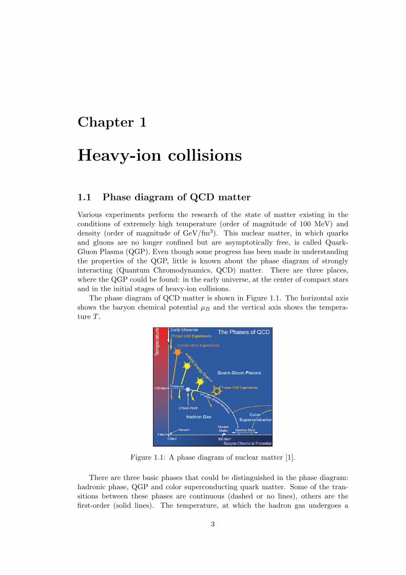
The phase diagram of QCD matter is shown in Figure 1.1. The horizontal axisshows the baryon chemical potential µB and the vertical axis shows the tempera-ture T .
Figure 1.1: A phase diagram of nuclear matter [1].
There are three basic phases that could be distinguished in the phase diagram:hadronic phase, QGP and color superconducting quark matter. Some of the tran-sitions between these phases are continuous (dashed or no lines), others are thefirst-order (solid lines). The temperature, at which the hadron gas undergoes a
3

1.2. SPACE-TIME EVOLUTION OF A NUCLEUS-NUCLEUS COLLISIONS
phase transition to QGP, is called the critical temperature Tc. Its value varies from150 to 170 MeV [24]. It can be seen, that at very low values of the baryon chemicalpotential, µB, lattice QCD calculations predict a smooth crossover transition, whileat higher values of µB, QCD-based models predict that there will be a first-orderphase transition between the QGP and hadron gas [25]. In order to clarify the struc-tures of the phase diagram, the Beam Energy Scan (BES) program at the RelativisticHeavy-Ion Collider (RHIC) is being preformed. The BES has three goals: search forthe turn off of the QGP signatures, search for the first-order phase transition, andsearch for the critical point (the end point of the first-order line).
1.2 Space-time evolution of a nucleus-nucleus collisions
High-energy hadron collisions can be considered in terms of two space-time scenarios,one of which was invented by Bjorken [26] and another by Landau [27]. Consider nowa central collision of two nuclei having a mass number A in the center-of-mass (CMS)frame with
√sNN = Ecm (see Appendix A). In this frame the nuclei are Lorentz-
contracted and collide having a thickness of d = 2R/γcm, where γcm = Ecm/2mN isthe Lorentz factor and mN is the nucleus mass.
Figure 1.2: A space-time view of a central collision of two heavy nuclei (A+A) in theLandau picture. a) Two nuclei approaching each other with relativistic velocitiesand zero impact parameter in the CMS frame. b) The slowing down of the nucleiwith further interaction and particle production. c) The light-cone representationof the high-energy hadron collision in the Landau picture. The shaded area is theparticle production area.
In the Landau picture (Figure 1.2), the colliding nuclei are considerably sloweddown, producing particles mainly within the thickness of nuclear matter. Then, theexpansion of the hot and baryon-rich system of particles occurs.
In the last decades, there is a considerable rise of the incident energy of the nuclei,the Landau model must be replaced by the Bjorken one (Figure 1.4). The Bjorkenscenario is based on the parton model of hadrons. It differs from the Landau pictureby the time expansion of particle production and the existence of wee partons (gluons
4

CHAPTER 1. HEAVY-ION COLLISIONS
and sea-quarks), which carry much smaller momentum fraction of the nucleon incomparison to valence quarks.
It is known, that after the two nuclei collide, the fireball is created, which under-goes different phases in its evolution. Figure 1.3 shows the space-time diagram ofthe relativistic collisions. The space-time evolution can be divided into three stages:pre-equilibrium stage and thermalization, hydrodynamical evolution and freeze-out,freeze-out and post-equilibrium [28].
Figure 1.3: A space-time evolution of the relativistic heavy-ion collision [2].
Pre-equilibrium stage and thermalization
Figure 1.4 shows a schematic view of a central collision of two heavy nuclei. Firstly,we see the two nuclei approaching each other with the relativistic velocities in thecenter of mass frame (Figure 1.4 a). As the collision is central, the value of theimpact parameter is zero. As soon as the nuclei pass through each other, the highlyexcited matter with a small net baryon number between the nuclei is left (shadedarea in Figure 1.4 b). After the significant number of the virtual quanta and gluoncoherent field configuration is excited, a proper time τde, typically a fraction of 1fm, is needed to de-excite these quanta into real quarks and gluons. The state ofmatter for 0 < τ < τde is called the pre-equilibrium stage. As the τde is definedin the rest frame of each quantum, the τ can be then defined as τ = τdeγ in thecenter of mass frame. The γ stands for the Lorentz factor of each quantum. Thisimplies the so called inside-outside cascade, meaning the slow particles are emergingfirst near the interaction point and then the fast particles far from the interactionpoint. This phenomenon is not included in the Landau model. In Figure 1.4 c thelight-cone representation of the nucleus-nucleus collision is shown. τ0 < τde standsfor the proper time within which the system is equilibrated and depends on thebasic parton-parton cross section and also on the density of partons produced in thepre-equilibrium stage.
5

1.2. SPACE-TIME EVOLUTION OF A NUCLEUS-NUCLEUS COLLISIONS
Figure 1.4: A space-time view of a central collision of two heavy nuclei (A + A) inthe Bjorken model. a) The central collision of two nuclei. b) Passage of the nucleithrough each other. c) The light-cone representation of the high-energy nucleus-nucleus collision. The shaded area is the area of forming the highly excited matter.
Hydrodynamical evolution and freeze-out
For this stage 0 < τ0 < τf , where τf stands for the freeze-out time of the hadronicplasma. In this period the evolution of the thermalized QGP and its phase transitionoccur. After the local thermal equilibrium is reached at τ0, the relativistic hydro-dynamics can be used for the description of the system expansion. The expectationvalues of the equations of the conservation of energy-momentum tensor and baryonnumber,
∂µ〈Tµν〉 = 0, ∂µ〈jµB〉 = 0, (1.1)
are taken with respect to the time-dependent state in the local thermal equilibrium[28]. In case the system is approximated as a perfect fluid, the local energy density,ε, and the local pressure, P , parametrize the expectation values. Therefore, theEquation (1.3) is supplemented by the equation of state ε = P (ε). Having theappropriate initial conditions at τ = τ0, the Equation (1.3) can predict the timedevelopment of the system until it undergoes a freeze-out at τ = τf . In other case,when the system cannot be approximated as a perfect fluid, the extra informationis required.
Freeze-out and post-equilibrium
For this stage τf < τ . A space-time hyper-surface defines the freeze-out of thehadronic plasma. As there is an increase of the mean free time of the plasmaparticles in comparison to the time scale of the plasma expansion, the local thermalequilibrium is no longer maintained. The freeze-out can be divided into 2 types.The first is the chemical freeze-out, after which the number of each species is frozen,while the equilibration in the phase-space is still maintained. The other one is thethermal equilibrium. In contradiction to the chemical freeze-out, after the thermalfreeze-out occurs, the kinetic equilibrium is no longer maintained. Besides, there
6

CHAPTER 1. HEAVY-ION COLLISIONS
could also be a difference in the temperature for the chemical and thermal freeze-outs. The first one should occur at higher temperature followed by the second one.After the evolution of the medium is finished, there is an increase in the distancesbetween the hadrons. Therefore, the hadrons leave the interaction region, but stillcan interact in a non-equilibrium way.
1.3 Centrality of the collision
1.3.1 Centrality types
Nuclear collisions can be classified according to the size of the overlapping area thatis related to centrality. Centrality can be determined as:
cb ≡1
σinnel
∫ b
0Pinel(b
′)2πb′db′, (1.2)
where σinel is the inelastic nucleus-nucleus cross section, Pinel is the probabilitythat an inelastic collision occurs at the impact parameter b that is defined as thedifference between the positions of the nuclei’s centers. Depending on the valuesof the impact parameter one can distinguish three types of collisions: central or”head-on” collisions, peripheral and ultra-peripheral collisions (Figure 1.5). Centralcollisions have the impact parameter b ≈ 0, peripheral collisions have 0 < b < 2R,and ultra-peripheral collisions have b > 2R, where the colliding nuclei are viewed ashard spheres with radius R.
Figure 1.5: A schematic view of central, peripheral and ultra-peripheral collisions.
The centrality dependence of various observables provides insight into their de-pendence on the global geometry. As the energy loss of partons increases with thelength of the path traversed inside the quark-gluon plasma, it is larger in centralcollisions.
1.3.2 Determination of centrality
In heavy-ion collisions the centrality of the collision and the impact parameter cannotbe directly experimentally measured, even though they are perfectly well-definedquantities. There are two main methods to determine the centrality.
7
1.3. CENTRALITY OF THE COLLISION
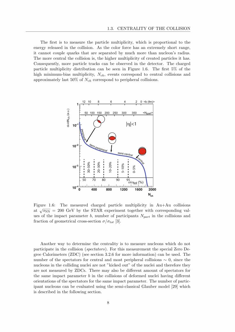
The first is to measure the particle multiplicity, which is proportional to theenergy released in the collision. As the color force has an extremely short range,it cannot couple quarks that are separated by much more than nucleon’s radius.The more central the collision is, the higher multiplicity of created particles it has.Consequently, more particle tracks can be observed in the detector. The chargedparticle multiplicity distribution can be seen in Figure 1.6. The first 5% of thehigh minimum-bias multiplicity, Nch, events correspond to central collisions andapproximately last 50% of Nch correspond to peripheral collisions.
Figure 1.6: The measured charged particle multiplicity in Au+Au collisionsat√sNN = 200 GeV by the STAR experiment together with corresponding val-
ues of the impact parameter b, number of participants Npart in the collisions andfraction of geometrical cross-section σ/σtot [3].
Another way to determine the centrality is to measure nucleons which do notparticipate in the collision (spectators). For this measurement the special Zero De-gree Calorimeters (ZDC) (see section 3.2.6 for more information) can be used. Thenumber of the spectators for central and most peripheral collisions ∼ 0, since thenucleons in the colliding nuclei are not ”kicked out” of the nuclei and therefore theyare not measured by ZDCs. There may also be different amount of spectators forthe same impact parameter b in the collisions of deformed nuclei having differentorientations of the spectators for the same impact parameter. The number of partic-ipant nucleons can be evaluated using the semi-classical Glauber model [29] whichis described in the following section.
8

CHAPTER 1. HEAVY-ION COLLISIONS
1.4 Glauber model of nucleus-nucleus collisions
In order to describe the high-energy nuclear reactions and evaluate the total reactioncross-section, the number of nucleons that participated in a binary collision at leastonce (participant nucleons), Npart, and nucleon-nucleon collisions, Ncoll, the Glaubermodel [29] is used. The Glauber model is a semi-classical model, which considers thenucleus-nucleus collision as multiple nucleon-nucleon interactions (see Figure 1.7).That means there is an interaction between the nucleon of the incident nucleus andthe target nucleons with a given density distribution. The nucleons are assumedto travel in the straight lines and are not deflected after the collision. That givesa good approximation at very high energies. As this model does not consider thesecondary particle production and possible excitations of nucleons, the nucleon-nucleon inelastic cross section, σinNN , is assumed to be the same as that in thevacuum.
Projectile B Target A
b zs
s-b
bs
s-b
a) Side View b) Beam-line View
B
A
Figure 1.7: Geometry of a collision between nucleus A and nucleus B. with trans-verse (a) and longitudinal (b) views [4].
In the Glauber model, the number of participant nucleons, Npart, and the numberof binary nucleon-nucleon collisions can be calculated as follows:
Npart(b) =
∫d2~sTA(~s)
(1− exp−σ
inNNTB(~s)
)+
∫d2~sTB(~s−~b)
(1− exp−σ
inNNTA(~s)
),
(1.3)
Ncoll(b) =
∫d2~sσinNNTA(~s)TB(~s−~b). (1.4)
Here, the TA is the thickness function defined as TA(s) =∫dzρA(z,~s),~b is the impact
parameter, ~s is the impact parameter of all pairs of incident and target nucleons, zis the collision axis and ρA is the nuclear mass number density normalized to massnumber A.
1.5 Hard probes of the QCD medium
In heavy-ion collisions the QGP exists only during the limited period of time (lessthan 10−23 seconds) and as a result of this, it cannot be studied directly. However,hard probes (heavy flavor quarks, jets) can be used for studying the properties of
9

1.5. HARD PROBES OF THE QCD MEDIUM
this medium as they are created early in the collision. In the following sections jetsand heavy flavor particles will be discussed.
1.5.1 Jets
In the early stages of nucleus-nucleus collisions a hard parton travelling throughthe Quark-Gluon Plasma emits gluons loosing thereby its energy. Such process isdescribed down to transfer momentum O(1) GeV by the Dokshitzer-Gribov-Lipatov-Altarelli-Parisi (DGLAP) evolution equation [30]
Q2∂fa(x,Q2)
∂Q2=∑b
∫ 1
x
dz
z
αs2πPab(z)fb(
x
z,Q2), (1.5)
where fa(x,Q2) is the parton distribution function (PDF), x is a fraction of a total
momentum, Q2 is the energy scale, αs is the running coupling constant, Pab isa splitting function1. The emitted gluons, in turn, produce qq pairs which thencombine together with the rest of free quarks into color charge neutral mesons andbaryons. As a result, a collimated spray of hadrons originating from fragmentationof a hard parton is formed which is called jet (Figure 1.8). As jets mostly conservethe energy and the direction of the originating parton, they are studied in orderto determine the properties of the original partons. If the parton does not haveenough energy, the jet will be quenched. Jets will be discussed in a more detail inthe following chapter.
Figure 1.8: A schematic view of jet created in a heavy-ion collision [5].
1.5.2 Heavy flavor
Using the term ”heavy flavor” one means the c, t and b quarks, as their masses aremuch larger then the QCD scale, ΛQCD, which is ≈ 218 MeV. The top quark is the
1Splitting function - the probability of a parton b splitting into a parton a with a momentumfraction z of the initial parton b.
10
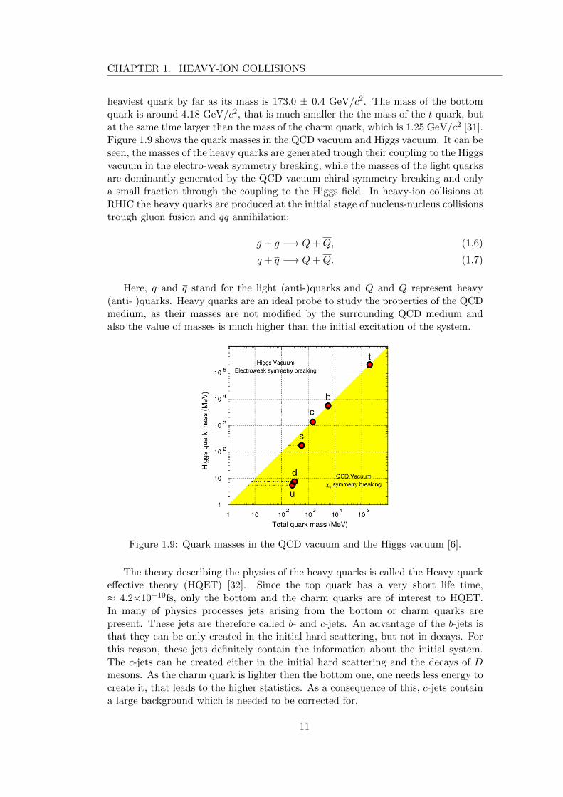
CHAPTER 1. HEAVY-ION COLLISIONS
heaviest quark by far as its mass is 173.0 ± 0.4 GeV/c2. The mass of the bottomquark is around 4.18 GeV/c2, that is much smaller the the mass of the t quark, butat the same time larger than the mass of the charm quark, which is 1.25 GeV/c2 [31].Figure 1.9 shows the quark masses in the QCD vacuum and Higgs vacuum. It can beseen, the masses of the heavy quarks are generated trough their coupling to the Higgsvacuum in the electro-weak symmetry breaking, while the masses of the light quarksare dominantly generated by the QCD vacuum chiral symmetry breaking and onlya small fraction through the coupling to the Higgs field. In heavy-ion collisions atRHIC the heavy quarks are produced at the initial stage of nucleus-nucleus collisionstrough gluon fusion and qq annihilation:
g + g −→ Q+Q, (1.6)
q + q −→ Q+Q. (1.7)
Here, q and q stand for the light (anti-)quarks and Q and Q represent heavy(anti- )quarks. Heavy quarks are an ideal probe to study the properties of the QCDmedium, as their masses are not modified by the surrounding QCD medium andalso the value of masses is much higher than the initial excitation of the system.
Figure 1.9: Quark masses in the QCD vacuum and the Higgs vacuum [6].
The theory describing the physics of the heavy quarks is called the Heavy quarkeffective theory (HQET) [32]. Since the top quark has a very short life time,≈ 4.2×10⁻¹⁰fs, only the bottom and the charm quarks are of interest to HQET.In many of physics processes jets arising from the bottom or charm quarks arepresent. These jets are therefore called b- and c-jets. An advantage of the b-jets isthat they can be only created in the initial hard scattering, but not in decays. Forthis reason, these jets definitely contain the information about the initial system.The c-jets can be created either in the initial hard scattering and the decays of Dmesons. As the charm quark is lighter then the bottom one, one needs less energy tocreate it, that leads to the higher statistics. As a consequence of this, c-jets containa large background which is needed to be corrected for.
11
1.6. NUCLEAR MODIFICATION FACTOR
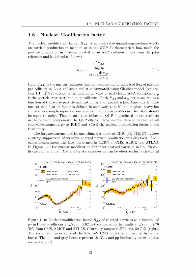
1.6 Nuclear Modification factor
The nuclear modification factor, RAA, is an observable quantifying medium effectson particle production in medium or in the QGP. It characterizes how much theparticle production in medium created in an A+A collision differs from the p+preference and is defined as follows:
RAA =
d2NAA
dpTdy
〈TAA〉d2σpp
dpTdy
. (1.8)
Here 〈TAA〉 is the nuclear thickness function accounting for increased flux of partonsper collision in A+A collisions and it is estimated using Glauber model (see sec-tion 1.4), d2NAA/dydpT is the differential yield of particles in A+A collisions, σpp
is the particle cross-section in p+p collisions. Both NAA and σpp are measured as afunction of transverse particle momentum pT and rapidity y (see Appendix A). Thenuclear modification factor is defined in such way, that if one imagines heavy-ioncollision as a simple superposition of individually binary collisions, then RAA shouldbe equal to unity. That means, that either no QGP is produced or other effectsin the collision compensate the QGP effects. Experimental data show that for alltransverse momenta pT at RHIC and STAR the nuclear modification factor is lessthan unity.
The first measurement of jet quenching was made at RHIC [33], [34], [35], wherea strong suppression of inclusive charged particle production was observed. Anal-ogous measurement was later performed in CERN at CMS, ALICE and ATLAS.In Figure 1.10 the nuclear modification factor for charged particles in Pb+Pb col-lisions can be found. A characteristic suppression can be observed for both central
(GeV)T
p1 10 210
AA
R
0
0.2
0.4
0.6
0.8
1
1.2
1.4
1.6
0-5%
and lumi. uncertaintyAAT|<1η|
(5.02 TeV PbPb)-1bµ (5.02 TeV pp) + 404 -127.4 pb
CMSCMS 5.02 TeV
CMS 2.76 TeV
ALICE 2.76 TeV
ATLAS 2.76 TeV
(GeV)T
p1 10 210
AA
R
0
0.2
0.4
0.6
0.8
1
1.2
1.4
1.6
50-70%
and lumi. uncertaintyAAT|<1η|
(5.02 TeV PbPb)-1bµ (5.02 TeV pp) + 404 -127.4 pb
CMSCMS 5.02 TeV
CMS 2.76 TeV
Figure 1.10: Nuclear modification factor RAA of charged particles as a function ofpT in Pb+Pb collisions at
√sNN = 5.02 TeV compared to the results at
√sNN = 2.76
TeV from CMS, ALICE and ATLAS. Centrality ranges: 0-5% (left), 50-70% (right).The systematic uncertainty of the 5.02 TeV CMS points is represented by yellowboxes. The blue and gray boxes represent the TAA and pp luminosity uncertainties,respectively. [7].
12

CHAPTER 1. HEAVY-ION COLLISIONS
(GeV/c)T
p0 2 4 6 8 10
0.5
1
1.5
0 D
LBT
Duke
D ALICE 2.76 TeV
= 200 GeV 0-10%NNsAu+Au (a)
(GeV/c)T
p0 2 4 6 8 10
0.5
1
1.5 0-12% STAR 200 GeV±π
0-5% ALICE 2.76 TeV±h
0-12% STAR 200 GeV±π
0-5% ALICE 2.76 TeV±h
(b)
AA
R
Figure 1.11: Upper panel: Nuclear modification factor for D0 mesons in centralAu+Au collisions at
√sNN = 200 GeV at STAR compared to the ALICE results at√
sNN = 2.76 TeV. Bottom panel: Measurements of charged pions from STAR andcharged hadrons from ALICE [8].
and peripheral collisions. For central collisions the suppression is around 7–8 for pT
6–9 GeV/c, that is much stronger than for peripheral ones.It is also important to look at production of heavy flavor particles described in
section 1.5.2. It is expected that particle composed of heavy-quarks will be lesssuppressed in nucleus-nucleus collisions due to their larger masses in comparison tolight quarks due to the dead-cone effect [36]. However, the measurements for D0
mesons, which contain charm quark, from STAR and ALICE show the suppressionis comparable to that of pions at both collision energies.
In order to obtain more detailed information about jet quenching the fully recon-structed jets are used. As jets are ”image” of the parton, their energy correspondsto the whole energy of the parton and therefore the less suppression is expected.The nuclear modification factor for jets can be defined similarly to the RAA of theparticles as
RAA =
1
Nevt
d2Njet
dpTdy
∣∣∣∣cent
〈TAA〉d2σjet
dpTdy
∣∣∣∣pp
(1.9)
where d2Njet/dpTdy is the differential jet yield, σjet is the jet cross-section in p+pcollisions and Nevt is the total number of A+A collisions within a chosen centralityinterval. Again, both Njet and σjet are measured as a function of transverse mo-
13

1.6. NUCLEAR MODIFICATION FACTOR
[GeV]T
p
AA
R
0.5
1
40 60 100 200 300 500 90040 60 100 200 300 500 90040 60 100 200 300 500 90040 60 100 200 300 500 90040 60 100 200 300 500 90040 60 100 200 300 500 90040 60 100 200 300 500 90040 60 100 200 300 500 90040 60 100 200 300 500 90040 60 100 200 300 500 900
0 - 10%20 - 30%40 - 50%60 - 70%
ATLAS = 5.02 TeVNNs = 0.4 jets, R tkanti-
| < 2.8y|-1 25 pbpp, -12015 data: Pb+Pb 0.49 nb
and luminosity uncer.⟩AA
T⟨
[GeV]T
p
AA
R
0.5
1
40 60 100 200 300 500 90040 60 100 200 300 500 90040 60 100 200 300 500 90040 60 100 200 300 500 90040 60 100 200 300 500 90040 60 100 200 300 500 90040 60 100 200 300 500 90040 60 100 200 300 500 90040 60 100 200 300 500 90040 60 100 200 300 500 900
10 - 20%30 - 40%50 - 60%70 - 80%
ATLAS = 5.02 TeVNNs = 0.4 jets, R tkanti-
| < 2.8y|-1 25 pbpp, -12015 data: Pb+Pb 0.49 nb
and luminosity uncer.⟩AA
T⟨
Figure 1.12: Nuclear modification factor RAA as a function of jet pT for jets with|y| < 2.8 in different centrality intervals. Right: 10-20%, 30-40%, 50-60%, 70-80%.Left: 0-10%, 20-30%, 40-50%, 60-70%. The pT of constituents is > 10 GeV/c. pT ofthe tracks > 10 GeV/c. The statistical uncertainties and the bin-wise correlated sys-tematic uncertainties are represented by the error-bars and the shaded boxes aroundthe data points, respectively. Fractional 〈TAA〉 and p+p luminosity uncertainties areshown as colored and grey shaded boxes, respectively, at RAA = 1 [9].
mentum of tracks pT and rapidity y. The measurement of fully reconstructed jetsis challenging due to large background and became really accessible at the LHCand recently also at RHIC due to large data samples. The results for high pT jetmeasurements at ATLAS (Figure 1.12) and CMS (Figure 1.10) show that in thesituation where in the jet cone more particles/energy is collected, still there is asuppression present for all centrality classes and jet radii.
3100
0.2
0.4
0.6
0.8
1
| < 2jet
η, |Tanti-k
R = 0.2
3100
0.2
0.4
0.6
0.8
1
R = 0.3
3100
0.2
0.4
0.6
0.8
1
R = 0.4
3100
0.2
0.4
0.6
0.8
1
R = 0.6
0-10%
10-30%AAT
3100
0.2
0.4
0.6
0.8
1
R = 0.8
30-50%
50-90%AAT
3100
0.2
0.4
0.6
0.8
1
R = 1.0
Lumi
200 1000 200 1000 200 10000
0.2
0.4
0.6
0.8
1
0
0.2
0.4
0.6
0.8
1
(GeV)jet
Tp
AA
R
PreliminaryCMS -1, pp 27.4 pb-1bµ = 5.02 TeV, PbPb 404 NNs
Figure 1.13: The RAA for jets as a function of pjetT for various resolution parametersand centrality classes [10].
14

CHAPTER 1. HEAVY-ION COLLISIONS
0 50 100)c(GeV/
T,jetp
0
0.2
0.4
0.6
0.8
1
1.2
1.4AA
R = 0.2RALICE
= 5.02 TeVNNsPb-Pb 0-10%
= 5.02 TeVspp
c> 5 GeV/lead,ch
Tp| < 0.5
jetη|
ALICE 0-10%
Correlated uncertainty
Shape uncertainty
0 50 100)c(GeV/
T,jetp
0
0.2
0.4
0.6
0.8
1
1.2
1.4AA
R = 0.4RALICE
= 5.02 TeVNNsPb-Pb 0-10%
= 5.02 TeVspp
c> 7 GeV/lead,ch
Tp| < 0.3
jetη|
ALICE 0-10%
Correlated uncertainty
Shape uncertainty
Figure 1.14: Jet RAA at√sNN = 5.02 TeV for R = 0.2 with |ηjet| < 0.5 (left) and
R = 0.4 with |ηjet| < 0.7 (right) [11].
Analogous measurements for lower jet transverse momenta and lower jet pT
constituents were performed by ALICE (Figure 1.14) and STAR (Figure 1.15) [12]for different resolution parameters of the jet. As there is no p+p reference at STAR,the ratio of the inclusive jet yields in central to peripheral collisions is used inorder to compare these two measurements. For this aim one can define the nuclearmodification factor, RCP , as follows:
RCP =
1Ncent
events
d2NcentdpT,jetdη
〈Nperibin 〉
1
Nperievents
d2Nperi
dpT,jetdη〈N cent
bin 〉. (1.10)
Both measurements show that the values of nuclear modification factor for all jetradii are approximately the same, RAA ≈ 0.4 at ALICE and RCP ≈ 0.45 at STAR.
Figure 1.15: Charged jet RCP with pleadT > 5 GeV for R = 0.2 - 0.4 [12].
15

1.6. NUCLEAR MODIFICATION FACTOR
16
Chapter 2
Jets
Jets can be divided into two groups: regular (”soft-resilient”) and less regular (”soft-adaptable”). Having a regular jet can simplify some theoretical calculations as wellas some parts of the momentum resolution loss caused by underlying event (UE) andpile-up contamination. An infrared and collinear (IRC) safe algorithm can stimulateirregularities in the boundary of the final jet in the second type of the jets.
2.1 Requirements for jet reconstructing algorithms
In order to reconstruct jets different algorithms are used. A good algorithm shouldsatisfy the following criteria:
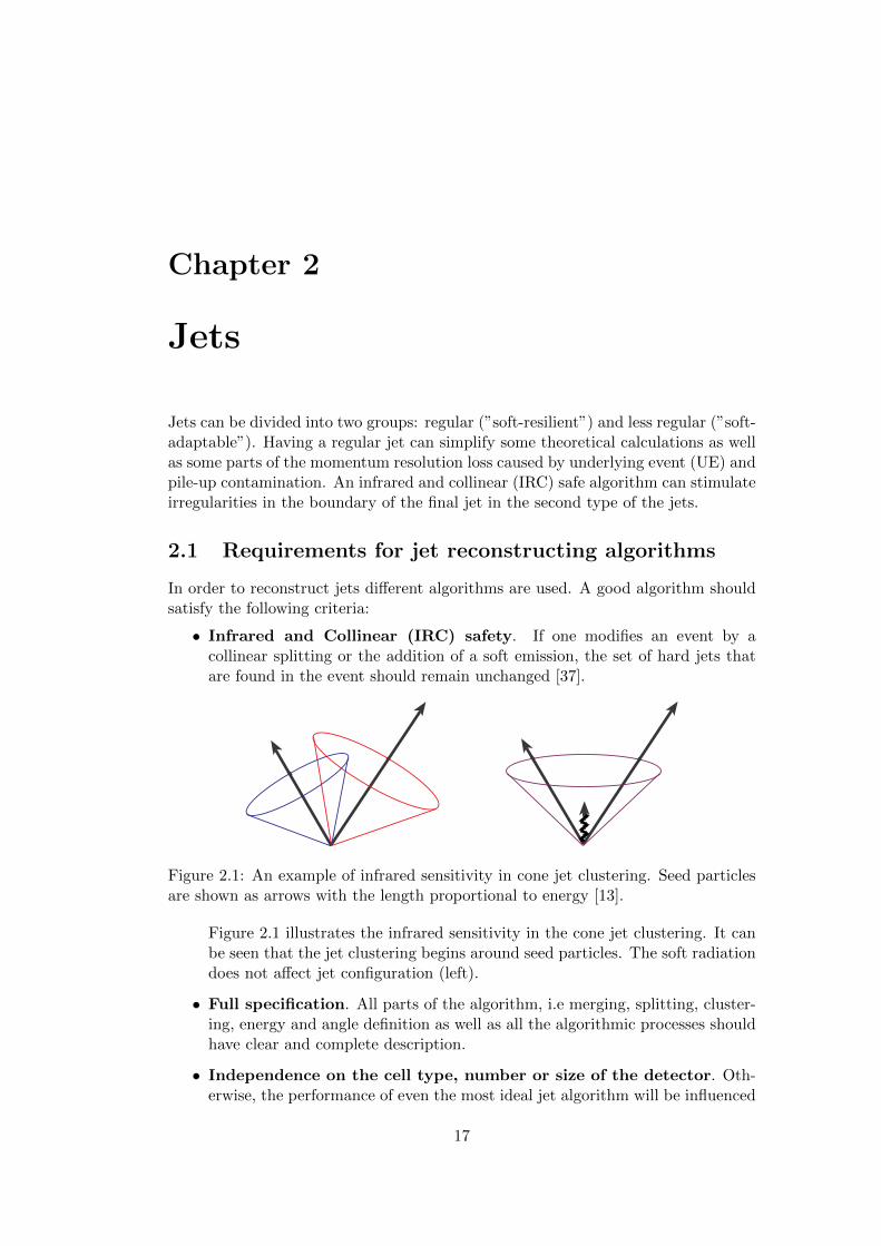
• Infrared and Collinear (IRC) safety. If one modifies an event by acollinear splitting or the addition of a soft emission, the set of hard jets thatare found in the event should remain unchanged [37].
Figure 2.1: An example of infrared sensitivity in cone jet clustering. Seed particlesare shown as arrows with the length proportional to energy [13].
Figure 2.1 illustrates the infrared sensitivity in the cone jet clustering. It canbe seen that the jet clustering begins around seed particles. The soft radiationdoes not affect jet configuration (left).
• Full specification. All parts of the algorithm, i.e merging, splitting, cluster-ing, energy and angle definition as well as all the algorithmic processes shouldhave clear and complete description.
• Independence on the cell type, number or size of the detector. Oth-erwise, the performance of even the most ideal jet algorithm will be influenced
17
2.2. SEQUENTIAL-CLUSTERING JET ALGORITHMS
by different effects, such as particle showering, noise, detector response afterthe jet enters a detector.
• Ease of use. The algorithms should be also easy to implement in perturbativecalculations, with typical experimental detectors and data.
• Order independence. The same results should be produced at the parton,particle and detector levels.
• High efficiency and short computing time. Computing time evolving asO(N3) should be the upper boundary for any practical use, where N standsfor the number of particles needed to be clustered.
Nowadays, there are two big classes of the jet finding algorithms: cone jet al-gorithms and sequential-clustering algorithms. The first type is based on identi-fying energy-flow into cones in pseudorapidity η = − ln tan θ
2 and azimuth φ (seeAppendix A). The second ones are based on successive pair-wise recombination ofparticles. The sequential recombination algorithms are infrared safe. As the cone jetalgorithms violate the IRC safety, this thesis will be focused on sequential-clusteringjet finding algorithms.
2.2 Sequential-clustering jet algorithms
The difference between the sequential recombination and cone jet finding methodsis in their sensitivity to non-perturbative effects like hadronization and underlyingevent (UE) contamination. Also, in comparison to the cone algorithms, the jetsreconstructed via sequential recombination have no fixed shape.
2.2.1 kT jet algorithm
For a set of particles with an index i having the transverse momentum kti, positionyi, φi the following steps are done.
1. Find the distance, dij , between particles i and j as
dij = min(k2ti, k
2tj)
∆2ij
R2. (2.1)
∆2ij = (yi − yj)2 + (φi − φj)2 and R is a radius parameter of the particle i.
2. Find the distance, diB, between the entity i and the beam B as
diB = k2ti. (2.2)
3. Find dmin = min(dij , diB).
4. If dmin = dij , merge the particles summing their four-momenta.
5. If dmin = diB, call a particle to be a final jet, remove it from the list.
6. Repeat the steps 1-5 until no particles are left.
18
CHAPTER 2. JETS
The main problem of the kT algorithm was originally its slowness. ClusteringN particles into jets requires O(N3) operations. However, this problem has beenalready solved (see section 2.4). As the kT algorithm is sensitive to the backgroundin comparison to other algorithms, it is mostly used for the background estimationin heavy-ion collisions.
2.2.2 Anti-kT jet algorithm
Contrary to the kT jet-finder, the anti-kT algorithm starts the clustering from thehardest particle (having the largest pT ). Then, all the steps are the same as for thekT algorithm. The only change is in the definitions of dij and diB. The first twosteps will be the following:
1. Find the distance, dij , between the hard particle and the remaining soft onesas
dij = min(k−2ti , k
−2tj )
∆2ij
R2. (2.3)
2. Find diB as
diB = k−2ti . (2.4)
The shape of the jet is determined only by the distance between the two hardparticles, ∆12, as the soft particle do not modify the jet shape. Overall, three casescould be distinguished:
1. There are no other hard particles within the distance 2R from the given hardparticle. Such a hard particle will collect all the soft particles around itselfinside a radius R. As a result a perfect conical jet will be acquired.
2. The second hard particle is located within a distance R < ∆12 <2R. Asa result, two hard jets will be obtained. The only difference will be in theshapes of these jets. Depending on the particle transverse momenta (kt1 andkt2) the following three cases could be distinguished:
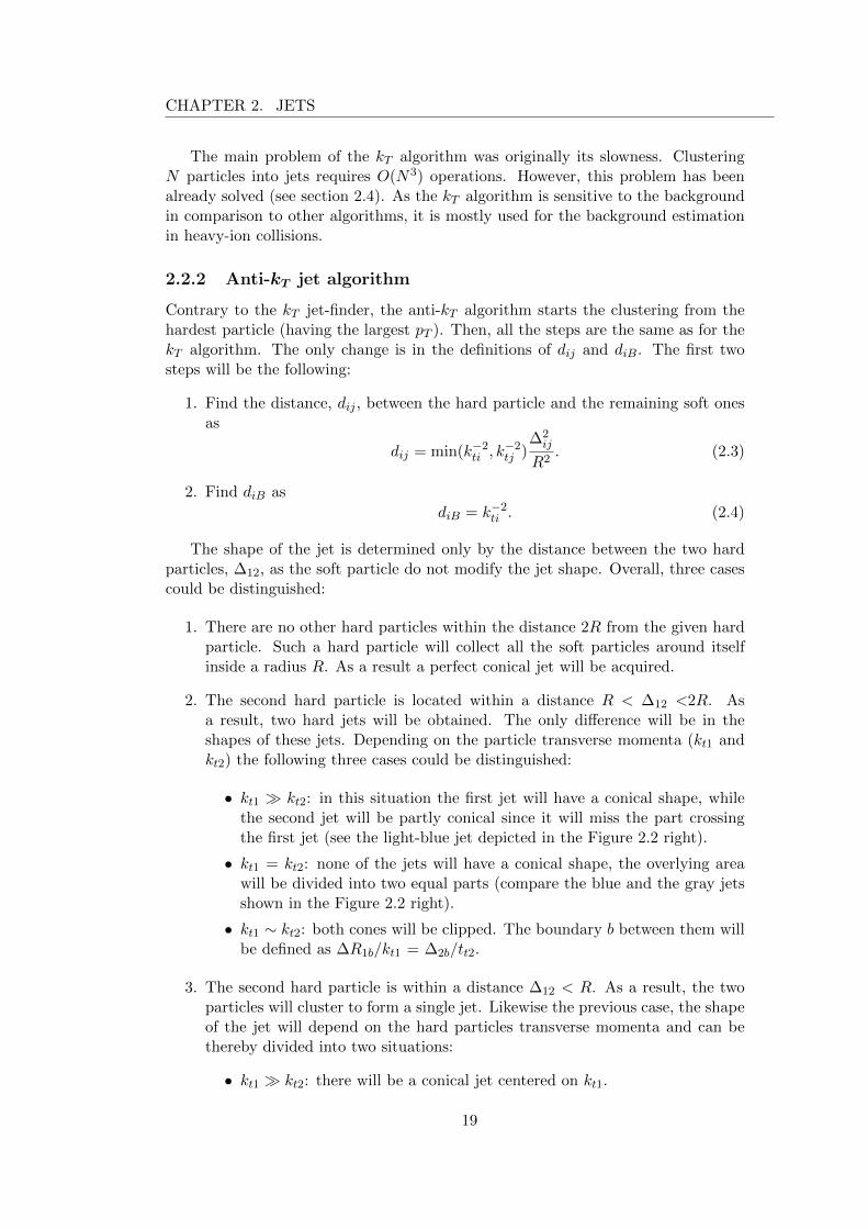
• kt1 � kt2: in this situation the first jet will have a conical shape, whilethe second jet will be partly conical since it will miss the part crossingthe first jet (see the light-blue jet depicted in the Figure 2.2 right).
• kt1 = kt2: none of the jets will have a conical shape, the overlying areawill be divided into two equal parts (compare the blue and the gray jetsshown in the Figure 2.2 right).
• kt1 ∼ kt2: both cones will be clipped. The boundary b between them willbe defined as ∆R1b/kt1 = ∆2b/tt2.
3. The second hard particle is within a distance ∆12 < R. As a result, the twoparticles will cluster to form a single jet. Likewise the previous case, the shapeof the jet will depend on the hard particles transverse momenta and can bethereby divided into two situations:
• kt1 � kt2: there will be a conical jet centered on kt1.
19
2.3. AREA RELATED PROPERTIES
Figure 2.2: A sample parton-level event generated with HERWIG Monte-Carlo gen-erator of p+p collision clustered with kT (left) and anti-kT (right) algorithms [14].
• kt1 ∼ kt2: the shape of the jet will be a union of cones having the radiusR around each hard particle plus a cone of radius R centered on the finaljet.
A comparison of the kT and anti-kT algorithm behavior is shown in Figure 2.2.A parton-level event was taken together with 104 soft particles and then clusteredwith the kT and the anti-kT algorithm, respectively. It can be seen, that for the kTalgorithm there are irregular shapes of jets, while the anti-kT algorithm gives jets ofthe regular shape.
2.3 Area related properties
In order to discuss the properties of jet boundaries for different algorithms, thecalculations of jet areas are used. The jet areas can be active or passive. The activejet area measures jet susceptibility to diffuse radiation and is defined as
A(J |{gi}) =Ng(J)
νg, (2.5)
where νg is the number of ghosts per unit area and Ng(J) is the number of ghostscontained in the jet J and {gi} is the given specific set of ghosts [38]. An exampleof such an area can be seen in the left part of Figure 2.2.
Passive area measures jet susceptibility to point-like radiation and can be calcu-lated using the following equation:
a(J) ≡∫dy dφ f(g(y, φ), J) f(g, J) =
{1 g ∈ J0 g /∈ J . (2.6)
That corresponds to the 4-vector area of the region where g is clustered with J
aµ(J) ≡∫dy dφ fµ(g(y, φ), J) fµ(g, J) =
{gµ/gt g ∈ J
0 g /∈ J , (2.7)
where gt is the ghost transverse momentum. In case of a jet with small area a(J), the4-vector area has the properties that its transverse component satisfies at(J) = a(J).
20

CHAPTER 2. JETS
0
2
4
6
8
10
0 0.5 1 1.5 2 2.5
(π R
2)/
N d
N/d
a
area/(πR2)
parton level
passive area
(a) SISCone
Cam/Aackt
anti-kt (x0.1)
0 0.5 1 1.5 2 2.50
2
4
6
8
10
(π R
2)/N d
N/d
A
area/(πR2)
hadron-level + pileup
active area
Pythia 6.4pt,min=1 TeV
2 hardest jets|y|<2, R=1
(b)
Figure 2.3: Distribution of areas in di-jet events at the LHC for various jet findingalgorithms. The events were generated by PYTHIA 6.4. (a) passive area at partonlevel, (b) active area at hadron level including UE and pile-up [14].
The area is also approximately massless and points in the direction of J . Otherwise,when the area of jet a(J)∼1, the 4-vector area receives a mass and may not pointin the same direction as J . For the typical IRC safe algorithm it is also importantto note that the jet passive area equals πR2 only when ∆12 = 0. Increasing ∆12
changes the area.
In Figure 2.3 the distributions of passive (left) and active (right) areas at partonand hadron levels respectively in di-jet events at the LHC can be observed. Thedistributions are calculated for cone jet algorithm SISCone [39] and three differentclustering jet algorithms (Cambridge/Aachen, kT and anti-kT ) using the PYTHIA6.4 Monte-Carlo generator.
2.4 FastJet
FastJet is a software package [14], [15], [40] containing most of jet finding algorithms.Besides, different tools for jet area calculation and background subtraction perfor-mance needed for various jet related analyses are also implemented in the package.
As it was discussed above, one of the main disadvantages of the kT algorithmused to be originally its slowness. This problem was solved in the implementation ofthe kT jet-finder in the FastJet package. Through the use of Voronoi diagrams [41]and a Delaunay triangulation for identification of each particles geometrical nearestneighbor, the geometrical aspects of the problem are isolated. The FastJet imple-mentation, therefore, reduces the kT algorithm complexity from (N3) to (N lnN)operations. Concerning this, the kT jet-finder can be used for large values of N thatrise when considering all cells of a finely segmented calorimeter and for heavy-ionevents. A comparison of the running times of the kT jet finding algorithm and itsFastJet implementation is depicted in Figure 2.4. It can be clearly seen that duringthe same time the FastJet implementation of the kT algorithm will cluster a largernumber of particles.
21

2.5. CONSTITUENT PILE-UP SUBTRACTION FOR JETS
Figure 2.4: The running times of the kT jet-finder and FastJet implementations ofthe kT clustering algorithm versus the number of initial particles [15].
2.5 Constituent pile-up subtraction for jets
Most jet shapes are significantly affected by pile-up, e.g. in high luminosity p+pcollisions or in heavy-ion collisions, which modifies kinematics of a jet. In orderto correct this effect different techniques are used. Simple ones remove a constant”offset” from the jets transverse momentum that is proportional to the number ofobserved pile-up effects, another methods subtracts an amount given by the productof the event’s measured pile-up pT density ρ and the jet’s measured area. In orderto correct the jet 4-momentum an area-based method [42] is used. It performs thecorrections after the jet finding has been accomplished. The method is based onthe measurement of each jet’s susceptibility to contamination, which is embodied inthe jet area A, from diffuse noise as well as on the measuring the level, ρ, of thisdiffuse noise in any given event. This method is also extended to account for hadronmasses. The area-based procedure allows to remove the contributions due to pileupeven for previously intractable jet shape observables, such as for example planarflow. Moreover, there is no need to have the explicit consideration of a specific jetalgorithm to perform the pileup subtraction.
The method is intended to be valid for arbitrary jet algorithms and generic IRCsafe jet shapes, without analytic study of each individual shape variable. Thus, itwill be discussed in more details below.
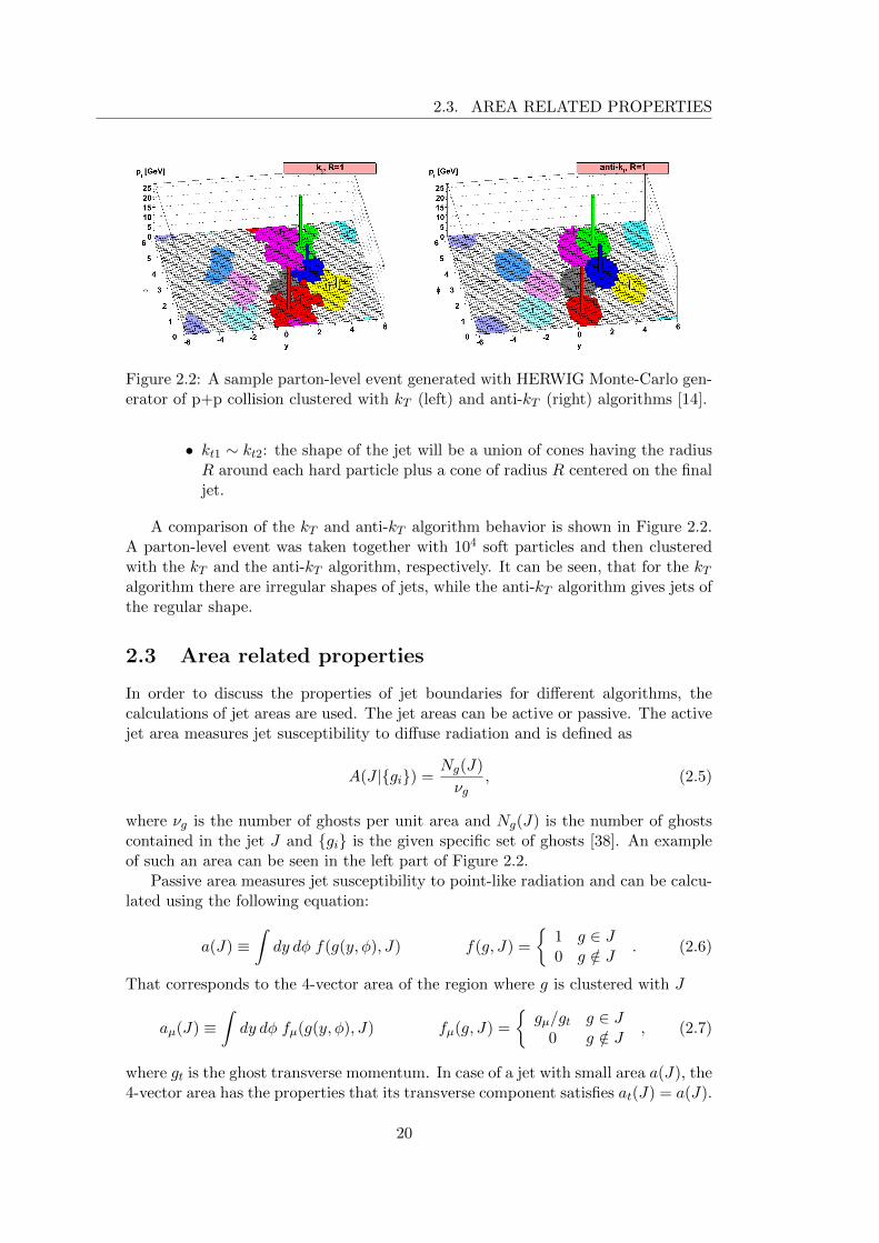
The first step is a characterization of the average pile-up density in a given eventterms of two variables - mass densities, ρ and ρm, such that the 4-vector of theexpected pile-up deposition, pµpileup, in a small region of size ∆y∆φ can be writtenas
pµpileup = [ρ cosφ, ρ sinφ, (ρ+ ρm) sinh y, (ρ+ ρm) cosh y]∆y∆φ. (2.8)
22
CHAPTER 2. JETS
Here ρ and ρm have only weak dependence on φ and y. In order to determine thesemass densities, all the particles are then grouped into so-called patches using the kTalgorithm. Then the ρ and ρm could be calculated as
ρ = medianpatches
{pT,patch
Apatch
}, (2.9)
ρm = medianpatches
{mδpatch
Apatch
}. (2.10)
Here, pT,patch and mδpatch are the transverse momentum and mass of each patch,respectively, and Apatch is the area of the patch in y − φ plane.
Further, it is necessary to include a set of very low momentum particles, so called”ghost particles”, that cover the y−φ plane with high density. Each of them coversa certain area Ag. The 4-momentum of the ghost particle could be expressed as
pµ = [pgT cosφ, pgT sinφ, (pgT +mgδ) sinh y, (pgT +mδ)
g cosh y], (2.11)
where mgδ =
√m2 + p2
T − pT and pgT is the transverse momentum of the ghost
particle. After the ghost particles are added to the event, the jet algorithm runsover all particles and ghosts. The same jets as in case without the ghost particles areproduced. That means that the jets now can be corrected for the pile-up. In orderto do so let us identify the transverse momentum and mass of the ghost particlewith the amount of pile-up within are Ag as
pgT = Ag · ρ, (2.12)
mgδ = Ag · ρm. (2.13)
Then, the specified amount of transverse momentum and mass is subtracted fromeach jet constituent using the matching scheme based on the distance between theparticle i and the ghost k, ∆Ri,k. This distance satisfy the following definition
∆Ri,k = pαT,i ·√
(yi − ygk)2 + (φi − φgk)2, (2.14)
where α could be any real number. If one wants to subtract the lower pT constituents,α should be set to 0. The list of the distances is then sorted in the ascending orderand the pile-up subtraction starts from the particle-ghost pair, which has the lowest∆Ri,k.
1. Correct the transverse momentum and mass of the particle and ghost as
If pTi ≥ pgTk pTi −→ pTi − pgTk,pgTk −→ 0;
otherwise: pTi −→ 0,
pgTk −→ pgTk − pTi.
∣∣∣∣∣If mδi ≥ mg
δk mδi −→ mδi −mgδk,
mgδk −→ 0;
otherwise: mδi −→ 0,
mgδk −→ mg
δk −mδi.
until the end of the list or the threshold, ∆Rmax is reached.
23

2.6. UNFOLDING TECHNIQUES
2. Discard the particles with the zero momentum. If no particle are left, the jetoriginates from pile-up.
3. Recalculate the 4-momentum of the jet.
The presence of the threshold in the algorithm guarantees the usage of only ghostsneighbouring the given particle to correct the kinematics of that particle. As theprocedure described above corrects the 4-momentum of a jet by constituent, it alsocorrects the substructure of a jet. This method corrects the jets only at the detectorlevel. In order to eliminate the detector effects, the unfolding techniques are used.
2.6 Unfolding techniques
In particle physics it is desired to have ”true” distributions, i.e the distributionsthat could be observed under the ideal conditions. However, such distributions arenever observed in real life. That is why, the ”observed” distribution is consideredas a ”noise distortion” of a ”true” one. One of the goals of the experimental physicsis to perform a separation of the true distribution from the observed spectrum. Forthis aim different techniques are used. In this thesis only two methods, Bayesianand SVD unfolding, will be described. These techniques are planned to be used infuture analysis [43], [44], [45].
2.6.1 Bayesian unfolding
Bayesian unfolding (or deconvolution) [43], [44] is based on the Bayes’ theorem whichallows to calculate the reverse probability form the known probability. Let us haveseveral independent causes (Ci, i = 1, 2, ..., nC) which can produce one effect (E). Ifthe initial probability of the causes, P (Ci), and the conditional probability of theith cause to produce the effect P (E|Ci) are known, then the Bayes formula can bedefined as
P (Ci|E) =P (E|Ci) · P0(Ci)nC∑l=1
P (E|Cl)P0(Cl)
. (2.15)
The initial probability P0(Ci) is called prior and the left side of the Equation (2.15) iscalled posterior. The probability P (E|Ci) is given by the response matrix, R[ptrue
T (i), pmeasT (j)]
= Rij , which satisfies the following condition: RC = E.Let us now denote contents of the bin Ej and Ci as n(Ej) and n(Ci), respectively.
Then, the best estimate is
n(Ci) =
nC∑j=1
n(Ej)P (Ci|Ej). (2.16)
Now, it is possible to estimate the true total number of the events, Ntrue, and thefinal probability of the causes, P (Ci) as
Ntrue =
nC∑i=1
n(Ci), (2.17)
P (Ci) ≡ P (Ci|n(E)) =n(Ci)
Ntrue
. (2.18)
24
CHAPTER 2. JETS
In case the prior is not consistent with the data, there will be no agreement withthe final distribution P (Ci). It is obvious that the smaller is the difference betweenthe initial and the true distributions, the better the agreement is. The Bayesianunfolding can be described as follows:
1. Choose the prior distribution P0(C) from the best knowledge of the processthat is studied. In case there is no information about the true distribution,then P0(Ci) is just a uniform distribution: P0(Ci) = 1/nC .
2. Calculate the unfolded distribution, n(C), and PC .
3. Perform a χ2 comparison between n(C) and n0(C).
4. Replace P0(C) with PC and n0(C) with n(C).
5. Start the process again. In case the value of the χ2 after the second iterationis small, stop the process. Otherwise, go to step 2.
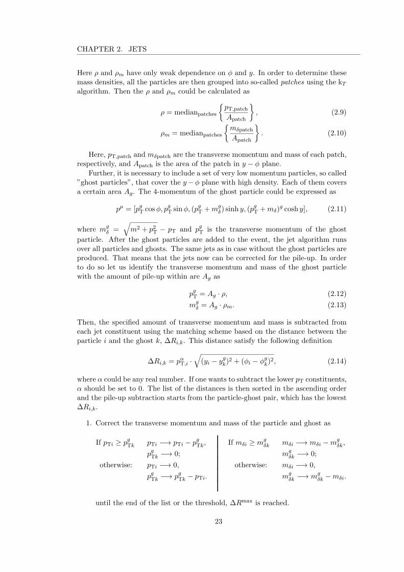
2.6.2 Singular Value Decomposition
A Singular Value Decomposition (SVD) [45] states that the response matrix R (realmatrix m× n) is its factorization of the form
R = USVT, (2.19)
where U and V are the orthogonal square matrices of m×m and n×n, respectively,and S is an m×n matrix with non-negative elements on the diagonal [45]. Thereforethe following relations are true:
UUT = UTU = I, (2.20)
VVT = VTV = I, (2.21)
Sij = 0 for i 6= j, Sij ≡ si ≥ 0. (2.22)
It was mentioned before, that the response matrix satisfies the following expression:RijCj = Ei. Using the Equation 2.19 one can get
USVT−→C =−→E . (2.23)
After the multiplication of this equation by UT from the right side one can obtain
SVT−→C = UT−→E . (2.24)
It is now possible to diagonalize this linear system by rotating the vectors d and z:
d ≡ UT−→E ,
z ≡ VT−→C
}⇒ si · zi = di ⇒ zi =
disi. (2.25)
It is very important to determine the zi correctly. Sometimes this process canfail due to several problems. First, when si is close to zero, then it leads to theincrease of the errors on di. Secondly, if E has large errors, then di is significant andhence the large error-bars can appear.
25

2.6. UNFOLDING TECHNIQUES
26
Chapter 3
RHIC and STAR
3.1 RHIC
The Relativistic Heavy Ion Collider (RHIC) is situated at Brookhaven NationalLaboratory. It is a ”chain” of different particle accelerators as can be seen fromFigure 3.1.
Figure 3.1: RHIC complex. 1 - Electron Beam Ion Source (EBIS), 2 - Linear Accel-erator (Linac), 3 - Booster Synchrotron, 4 - Alternating Gradient Synchrotron, 5 -AGS-to-RHIC Line, 6 - RHIC [1].
Heavy-ions start the movement from the Electron Beam Ion Source accelerator(1), which is a compact source and heavy-ion accelerator. It serves as the start ofthe pre-injector system for RHIC and can create highly charged ion beams fromalmost any element. The ion beams are later accelerated in two small Linacs (2)and then carried to the circular Booster synchrotron (3). The Booster providesthe ions with more energy. Ions move forward with higher and higher speed andthen enter the Alternating Gradient Synchrotron (AGS) (4) at an approximately37% speed of light. After the acceleration in the AGS the beam travels through
27

3.2. STAR
the AGS-to-RHIC Line (5) at 99.7% of the speed of light. At the end of this line aswitching magnet sends the ion bunches down to one of the two beam lines, such thatthe bunches are directed right to the counter-clockwise RHIC direction and left tothe clockwise RHIC direction, respectively. These beams are accelerated, as in theBooster Synchrotron or AGS, and then circulate in RHIC where they would collide insix interaction points. At four of the six interaction points a detector is/was located.There are PHOBOS (10 o’clock interaction point), BRAHMS (2 o’clock interactionpoint), STAR (6 o’clock interaction point) and PHENIX/sPHENIX, that will be atthe 8 o’clock interaction point. The first two experiments finished the data collection11 years ago. Super PHENIX (sPHENIX) will be a new experiment that is proposedto replace the PHENIX experiment that completed its last measurements in 2016.
3.2 STAR
The Solenoidal Tracker at RHIC (STAR) is an experiment that studies the for-mation and characteristics of QGP and also origin of the spin of the proton. It isdesigned to detect particles that arise as a result of the interaction of ultrarelativis-tic heavy-ions or protons. The STAR detector system is shown in Figure 3.2. Incentral Au+Au collisions at
√sNN = 200 GeV more than 1000 particles are formed.
Much more particles appear due to the decay of the short-lived particles and theinteraction of primary particles with the detector material. In order to identify eachof these particles and to determine the trajectories, different types of calorimeters,detectors and counters are used.
Figure 3.2: A 3D model of the STAR detector system [16].
The Time Projection Chamber (TPC) is the main part of the system to measurecharged particle tracks after collisions. The Barrel and Endcap Electro-MagneticCalorimeters (BEMC and EEMC) allow to measure hadronic and photonic energydeposition in the calorimeter towers. The Beam-Beam Counter (BBC), Vertex
28

CHAPTER 3. RHIC AND STAR
Position Detector (VPD) and Zero-Degree Calorimeter (ZDC) are used to monitorcollision luminosity and beam polarimetry. The Time Of Flight detector (TOF) ofSTAR is designed for improvement of direct identification of hadrons. The HeavyFlavor Tracker reconstructs open heavy flavor hadrons with displaced decay verticesenhancing thereby many open heavy flavor measurements.
3.2.1 Time Projection Chamber
The TPC is the central part of the STAR detector system. It is a cylindrical detectorwith 4 m in diameter and 4.2 m in length built around the beam-line. The detectoris filled with gas in a well-defined, uniform, electric field of ≈ 135 V/cm. Electricallycharged particles, that were produced in high-
√s heavy-ion collisions, are deflected
by the STAR magnet in a helical motion.
The TPC acceptance coverage is 2π in azimuthal angle φ and −1 < η < +1in pseudorapidity. The TPC has been recently upgraded with inner TPC (iTPC)having −1.3 < η < +1.3, which has started taking data in 2019. The upgrade pro-vides better momentum resolution and improved acceptance at high pseudorapidityto |η| < 1.7. The layout of the STAR TPC is shown in Figure 3.3. It consists of acentral membrane, an inner and outer field cage and two end-cap planes. The emptyspace between the central membrane and two end-caps is filled with P10 gas, whichis 10% methane and 90% argon regulated at 2 mbar above atmospheric pressure.After the passage of the charged particles through the gas, the ionized secondaryelectrons drift toward the two end-caps in the uniform electric field which is pro-vided by the two end-caps and the central membrane. The drifting electrons arethen collected by the end-caps.
The TPC is able to record these tracks, measure their momenta and identify
Figure 3.3: The layout of the STAR Time Projection Chamber [17].
29

3.2. STAR
particles by their ionization energy loss (dE/dx), which is calculated using the Bethe-Bloch formula [46]
−dEdx
= 4πNAr2emec
2z2 Z
Aβ2
(1
2ln
2mec2β2γ2TmaxI2
)− β2 − δ
2− 2
C
Z. (3.1)
Here, NA is the Avogadro number, re is classical electron radius, me is the massof the particle that losses energy, z is the charge of the incoming particle, ρ ismaterial density, Tmax is maximum energy transfer in a single collision, I is themean excitation energy, Z and A are the proton number and relative atomic mass,respectively, δ and C are the density and shell corrections. Figure 3.4 shows thetrack energy loss measured by the TPC in 200 GeV Au+Au collisions for differentparticle species associated to the observed bands.
Figure 3.4: The ionization energy loss measured in 200 GeV Au+Au collisions atRHIC [18].
3.2.2 Barrel Electro-Magnetic Calorimeter
The Barrel Electro-Magnetic Calorimeter (BEMC) is a fast lead-scintillator, sam-pling electromagnetic calorimeter. It surrounds the Central Trigger Barrel and theTPC. The BEMC allows STAR the triggering and studying of the high-pT processes,e.g. jets, heavy quarks, due to its acceptance that is equal to that of the TPC forfull length tracks (Figure 3.5). The coverage region of the calorimeter is −1 < η < 1in pseudorapidity and 2π in azimuth angle. The calorimeter is divided into 120segments in φ and 40 segments in η. That means there are 4800 calorimetric tow-ers in total, each tower having its individual readout. Resolution of the BEMC is0.05 × 0.05 (∆×∆η).
30

CHAPTER 3. RHIC AND STAR
Figure 3.5: Cross sectional views of the STAR detector. The Barrel EMC covers|η| ≤ 1. The BEMC modules slide in from the ends on rails which are held byaluminum hangers attached to the magnet iron between the magnet coils [19].
Figure 3.6: A side view of the STAR BEMC module. The image shows the location ofthe two layers of shower maximum detector at a depth of approximately 5 radiationlength X0 from the front face at η = 0 [19].
31

3.2. STAR
The neutral energy in the form of produced photons can be measured by de-tecting the particle cascade when those photons interact with the calorimeter. Thecalorimeter stack is stable in any orientation due to the friction between individuallayers.
In order to get precise measurements for π0’s and direct photons the shower max-imum detectors are implemented in the BEMC situating approximately 5 radiationlengths from the front of the stack. That provides the high the spatial resolutionmeasurements of shower distributions in two mutually orthogonal transverse dimen-sions.
An end view of a module showing the mounting system and the compressioncomponents is shown in Figure 3.6.
3.2.3 Endcap Electro-Magnetic Calorimeter
The Endcap Electro-Magnetic Calorimeter (EEMC) is a lead-scintillator samplingelectromagnetic calorimeter that covers the west endcap of the Time ProjectionChamber as it is depicted in Figure 3.7. There are 720 individual towers groupedtogether to provide coverage for pseudorapidity values 1 < η ≤ 2 and full azimuthrange. The EEMC significantly enhances STAR’s sensitivity to the flavor depen-dence of sea antiquark polarizations via W± production in polarized p+p collisions.
Figure 3.7: Endcap Electro-Magnetic Calorimeter [16].
3.2.4 Beam-Beam Counter
The Beam-Beam Counter (BBC) is a set of scintillator rings installed around theRHIC beam pipe on the east and west pole tips of the STAR magnet. The schematicview of its positions is depicted in Figure 3.8.
Each BBC counter consists of two rings of hexagonal scintillator tiles. An outerring is composed of large tiles and an inner ring is composed of small tiles. Eachof these annuli is internally divided into two separate subrings of 6 and 12 tileseach [16]. The hexagonal tile annuli for BBC is depicted in Figure 3.9.
32

CHAPTER 3. RHIC AND STAR
Figure 3.8: The schematic view of the BBC position. The blue and yellow arrowsrepresent the differently polarized proton beams.
Figure 3.9: A schematic view of the Beam-Beam Counter [16].
3.2.5 Vertex Position Detector
The Vertex Position Detector (VPD) consits of two detectors, one of which locatedon the east and another on the west side of the STAR. The VPD provides the primarydetector input to STAR minimum bias trigger in heavy-ion collisions. Both VPDcontains nineteen detectors, a schematic side view of which is shown in Figure 3.10.Approximately half of the solid angle in the pseudorapidity range of 4.24 ≤ η ≤ 5.1is subtended by all of the nineteen detectors in each assembly. There are up tonineteen times measured by the VPD in each event. These times are then used forthe calculation of the primary vertex along the beam pipe position zvtx via
Zvtx = c(Teast − Twest)/2, (3.2)
where c is the speed of light, Teast and Twest are the times from each of the twoVPDs. The times measured by the Vertex Position Detector are also needed for thestart time Tstart calculation as
Tstart = (Teast + Twest)/2− L/c, (3.3)
where L is the distance between the center of STAR and each VPD. The start timeis lately used by the TOF to perform particle identification at mid-rapidity.
3.2.6 Zero-Degree Calorimeter
The Zero-Degree Calorimeter (ZDC) is a small transverse area hadron calorimeterlocated downstream of the DX dipole magnets in STAR. This detector measures
33

3.2. STAR
�
�
�
�
�
�
�
�
�
�
Base R5946 PMT scint Pb
electrostatic shieldKapton tape
RTV-615lead wirespacerback cap
front cap
BNC
SHV
Figure 3.10: A schematic side view of the Vertex Position Detector [20].
neutral particles energy within a 2 mrad cone about the beam direction. The de-tector is specially designed for the requirements of Au+Au runs. However, it is alsoused for the p+Au and p+p runs. The energy measurement in essence counts thenumber of free ”spectator” neutrons that is used for the event-by-event characteri-zation. The effective cross-section of the ZDC coincidence rate during the 200 GeVAu+Au collisions is approximately 10.4 barns [47].
Figure 3.11: RHIC Zero-Degree Calorimeter [16].
The two ZDCs are located at the first bending magnets in the collider line, 18 maway from the geometry center of the STAR detector. Each of the two calorimetersis split into three modules that consist of layers of lead in scintillator fibers going toa Photomultiplier (PMT) and Analog-to-Digital Converters (ADC). The determined
34

CHAPTER 3. RHIC AND STAR
number of spectator neutrons is then used as a minimum bias trigger.
3.2.7 Time Of Flight
The Time Of Flight (TOF) detector, depicted in Figure 3.12, measures time in-tervals with a specific precision. While the VPD measures the ”start time” of theparticle, the TOF measures the so-called stop time of the particle. The difference,∆t, between these times is the time of flight of the particle. Using the data fromthe TPC the inverse velocity 1/β for each track and the particle mass M can becalculated as
1
β= c
∆t
s, (3.4)
M = p
√1
β2− 1, (3.5)
where s is the total path length, p is the momentum and c is the speed of light.
Figure 3.12: The TOF system [16].
The momentum dependence of the particle mass resolution for a 100 ps timeresolution for pions, kaons, deuterons and protons is shown in Figure 3.13. The upperline in the pair shows the dependence of M + ∆M versus the momentum. The M −∆M dependence on the momentum is demonstrated by the lower line. An exampleof particle identification with the TOF from Au+Au collisions at the top RHICenergy is shown in Figure 3.14. It can also be seen from this figure that with theincreasing momentum pions are the first particles leading to a significant backgroundin the proton identification and the first background to deuteron identification.
The TOF system can provide direct K, p or π identification up to momentap ∼ 1.7 GeV/c, proton identification up to p ∼ 2.6 GeV/c, deuteron identificationout to p ∼ 4 GeV/c [21].
35
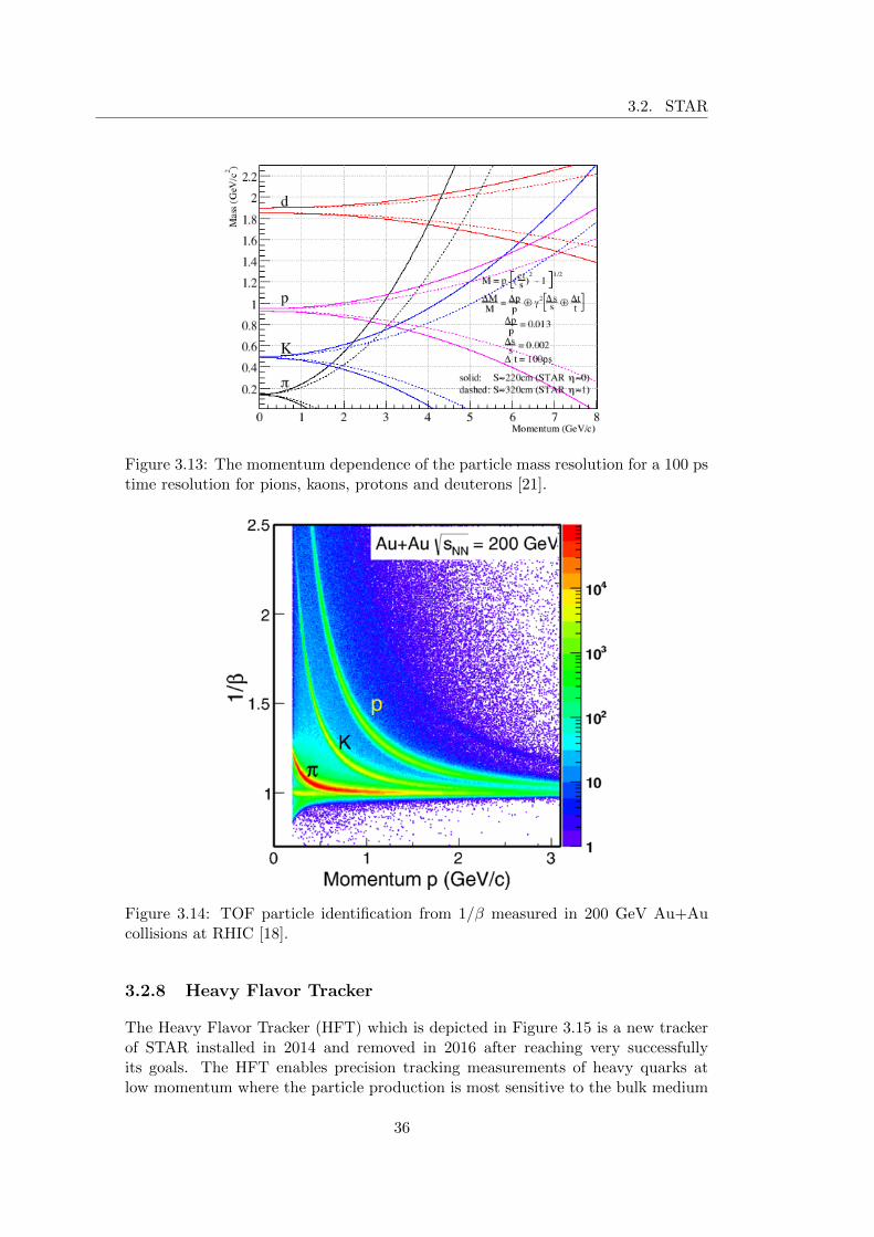
3.2. STAR
Figure 3.13: The momentum dependence of the particle mass resolution for a 100 pstime resolution for pions, kaons, protons and deuterons [21].
Figure 3.14: TOF particle identification from 1/β measured in 200 GeV Au+Aucollisions at RHIC [18].
3.2.8 Heavy Flavor Tracker
The Heavy Flavor Tracker (HFT) which is depicted in Figure 3.15 is a new trackerof STAR installed in 2014 and removed in 2016 after reaching very successfullyits goals. The HFT enables precision tracking measurements of heavy quarks atlow momentum where the particle production is most sensitive to the bulk medium
36

CHAPTER 3. RHIC AND STAR
created in heavy-ion collisions. The HFT allows to distinguish the decay vertices ofheavy flavor particles from primary vertices and significantly reduces combinationalbackground, which yields cleaner measurements with a higher level of significance.
Figure 3.15: A schematic view of the Heavy Flavor Tracker inside the STAR detector[16].
There are three detectors that compose the Heavy Flavor Tracker: a silicon pixeldetector (PXL), a double-sided Silicon Strip detector (SSD) and an IntermediateSilicon Tracker (IST). The HFT structure is shown in Figure 3.16. Since the minimalradius of the HFT is only 2.5 cm, it tightly surrounds the beam pipe. The SPD andthe IST lie inside the radial location of the SSD. The Intermediate Silicon Trackeris a single-sided double-metal silicon pad detector that matches the high resolutionof the PXL with the high resolution of the Time Projection Chamber and the SSD.The IST is composed of two layers. The inner layer lies at a radius of 12 cm andconsists of 19 ladders of 40 cm length [48]. The outer layer lies at a radius of 17 cmand consists of 27 ladders of 52 cm length. The strips on the inner layer are orientedto give the best resolution in the r − φ direction, while the strips of outer layer areoriented to give the best resolution in the z direction.
The HFT Pixel Detector is the first operational vertex detector based on Mono-lithic Active Pixel Sensors (MAPS) or also called CMOS Pixel Sensors (CPS). Itis a low mass detector located closest to the beam pipe. For this reason, the PixelDetector achieves the maximum resolution. As the IST, the PXL is also composedof two layers. The inner layer is located at a radius of 2.5 on average radius and has9 ladders. The outer one is located at a 7 cm radius and consists of 24 ladders.
37

3.2. STAR
Figure 3.16: The Heavy Flavor Tracker parts. PXL - Pixel Detector, IST - Interme-diate Silicon Tracker, SSD - double-sided Silicon Strip Detector [16].
38

Chapter 4
Contribution to the ForwardCalorimeter System Upgrade
4.1 Forward Calorimeter System
During my one-month stay at BNL, I was participating in the Forward CalorimeterSystem Upgrade. During this period I have helped in different projects. Their aimsas well as the results of my work will be described in more detail below.
In order to explore QCD physics in the high and low region of Bjorken x, theSTAR Forward Calorimeter System (FCS) upgrade is planned. In Figure 4.1 a
Figure 4.1: A three-dimensional CAD model of the FCS in the STAR detectormodel [22].
39

4.2. HCAL SCINTILLATING TILES
scheme of the FCS is shown. The FCS will consist of a Spaghetti ElectromagneticCalorimeter (SPACal), followed by a lead and scintillator plate sampling HadronicCalorimeter (HCal). For the Electromagnetic Calorimeter (ECal) it was decided totake the calorimeter from the PHENIX experiment after the end of the data takingin 2016 as it has the required energy resolution and therefore constitutes a verycost-effective solution. The refurbished read-out system will be placed in the frontin order to minimize the dead gaps between the ECal and the HCal.
4.2 HCal scintillating tiles
The new hadronic calorimeter will have 18720 scintillating tiles. The tiles should bepolished and painted before they will be installed in the HCal. These procedures aredone by different universities. The size of each tile is 95×97 mm×mm. The longerside was polished, while the short one was painted. Previous team of three peoplehad spent 35 hours to polish and paint 600 tiles. As the painting have been doneseparately for each tile, it was decided to change the technique by using clamps.That had reduced the time of the machining, so it took approximately 25 hours topolish and paint the batch of 600 tiles by two people.
In order to distinguish the long side from the short one, all the tiles have beenmarked. The polypad is placed on the rotating table of the polisher, which is set tospin at moderate speed. Then it is wet with water dripping at a very slow rate fromthe tap situated at the back side of the polisher. Afterwards, a small amount of thefine scratch remover is placed in the center of the polypad. As it is hard to keep onetile perpendicular to the surface of the polisher, it was decided to use a stack of 6or 7 tiles to have a better feeling when the tiles tilt. All the equipment used for thepolishing procedure is shown in Figure 4.2.
After the polishing the surface and edges of each tile are wiped and the stackis visually inspected to ensure that polishing is complete. A significant difference
Figure 4.2: The polisher: CrystalMaster Pro 12 Lap Grinder Kit (left) and theNOVUS fine scratch remover (right).
40
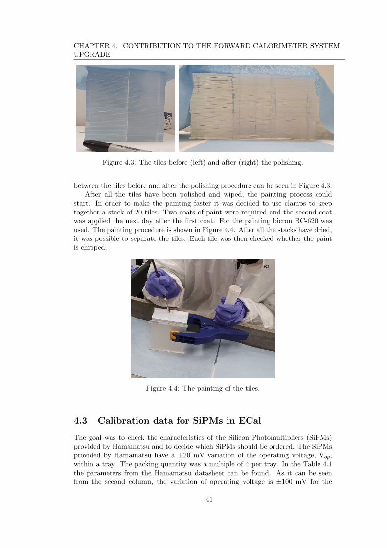
CHAPTER 4. CONTRIBUTION TO THE FORWARD CALORIMETER SYSTEMUPGRADE
Figure 4.3: The tiles before (left) and after (right) the polishing.
between the tiles before and after the polishing procedure can be seen in Figure 4.3.
After all the tiles have been polished and wiped, the painting process couldstart. In order to make the painting faster it was decided to use clamps to keeptogether a stack of 20 tiles. Two coats of paint were required and the second coatwas applied the next day after the first coat. For the painting bicron BC-620 wasused. The painting procedure is shown in Figure 4.4. After all the stacks have dried,it was possible to separate the tiles. Each tile was then checked whether the paintis chipped.
Figure 4.4: The painting of the tiles.
4.3 Calibration data for SiPMs in ECal
The goal was to check the characteristics of the Silicon Photomultipliers (SiPMs)provided by Hamamatsu and to decide which SiPMs should be ordered. The SiPMsprovided by Hamamatsu have a ±20 mV variation of the operating voltage, Vop,within a tray. The packing quantity was a multiple of 4 per tray. In the Table 4.1the parameters from the Hamamatsu datasheet can be found. As it can be seenfrom the second column, the variation of operating voltage is ±100 mV for the
41

4.3. CALIBRATION DATA FOR SIPMS IN ECAL
Type No. S14160-9401
Shipping date 31.07.2019
T[◦C] 25
Tray No. Vop Range, [V] Quantity, [pcs]
1 41.73 - 41.76 68
2 41.77 - 41.80 156
3 41.77 - 41.80 20
4 41.81 - 41.84 156
5 41.81 - 41.84 52
6 41.85 - 41.88 156
7 41.85 - 41.88 136
8 41.89 - 41.92 156
9 41.89 - 41.92 100
Table 4.1: The parameters provided by Hamamatsu.
Figure 4.5: The SiPM boards used for data taking.
whole sample. For the calibration the data taken at UCLA for pre-production batchof SiPMs was used. The SiPM boards that were used for taking data can be seenin Figure 4.5. These boards have been glued for the first four rows of towers in therecently stacked EMcal.
Figure 4.6 shows the dependence of current on the bias voltage for all SiPMboards. The given current is shown with a green line. The corresponding rangefor the bias voltage is shown with red lines. It can be seen, that all of them havelinear dependence (except the one board only). For the given current (159 µA) thebias voltage is 39.82 V ± 100 mV, that is roughly consistent with data provided byHamamatsu.
42
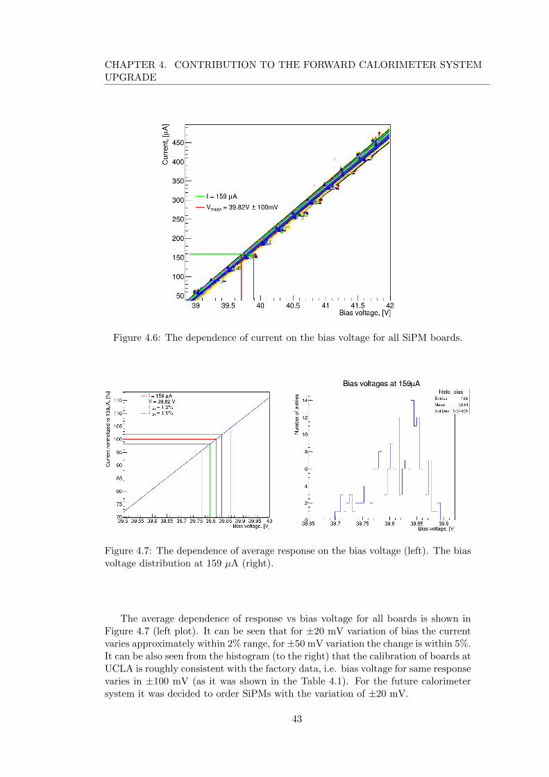
CHAPTER 4. CONTRIBUTION TO THE FORWARD CALORIMETER SYSTEMUPGRADE
Figure 4.6: The dependence of current on the bias voltage for all SiPM boards.
Figure 4.7: The dependence of average response on the bias voltage (left). The biasvoltage distribution at 159 µA (right).
The average dependence of response vs bias voltage for all boards is shown inFigure 4.7 (left plot). It can be seen that for ±20 mV variation of bias the currentvaries approximately within 2% range, for±50 mV variation the change is within 5%.It can be also seen from the histogram (to the right) that the calibration of boards atUCLA is roughly consistent with the factory data, i.e. bias voltage for same responsevaries in ±100 mV (as it was shown in the Table 4.1). For the future calorimetersystem it was decided to order SiPMs with the variation of ±20 mV.
43
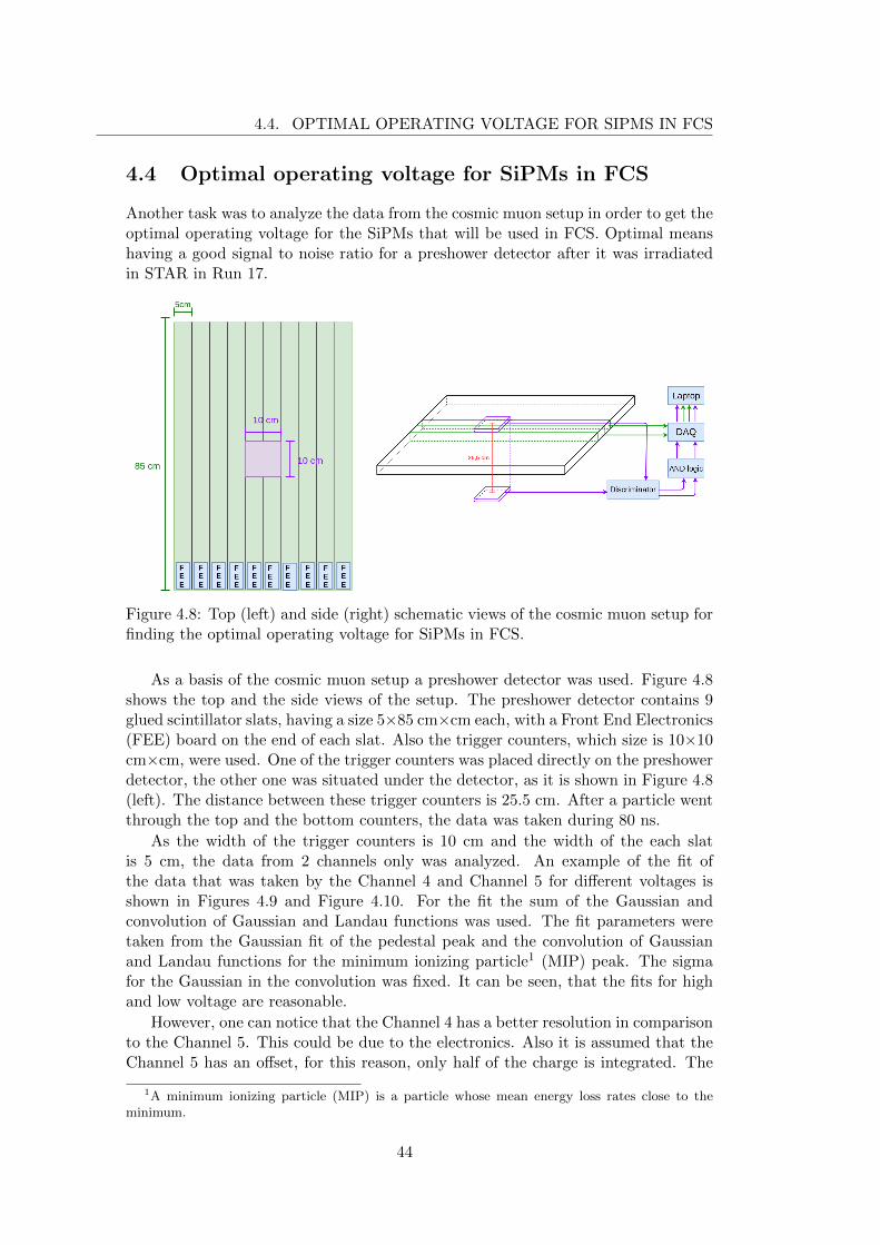
4.4. OPTIMAL OPERATING VOLTAGE FOR SIPMS IN FCS
4.4 Optimal operating voltage for SiPMs in FCS
Another task was to analyze the data from the cosmic muon setup in order to get theoptimal operating voltage for the SiPMs that will be used in FCS. Optimal meanshaving a good signal to noise ratio for a preshower detector after it was irradiatedin STAR in Run 17.
Figure 4.8: Top (left) and side (right) schematic views of the cosmic muon setup forfinding the optimal operating voltage for SiPMs in FCS.
As a basis of the cosmic muon setup a preshower detector was used. Figure 4.8shows the top and the side views of the setup. The preshower detector contains 9glued scintillator slats, having a size 5×85 cm×cm each, with a Front End Electronics(FEE) board on the end of each slat. Also the trigger counters, which size is 10×10cm×cm, were used. One of the trigger counters was placed directly on the preshowerdetector, the other one was situated under the detector, as it is shown in Figure 4.8(left). The distance between these trigger counters is 25.5 cm. After a particle wentthrough the top and the bottom counters, the data was taken during 80 ns.
As the width of the trigger counters is 10 cm and the width of the each slatis 5 cm, the data from 2 channels only was analyzed. An example of the fit ofthe data that was taken by the Channel 4 and Channel 5 for different voltages isshown in Figures 4.9 and Figure 4.10. For the fit the sum of the Gaussian andconvolution of Gaussian and Landau functions was used. The fit parameters weretaken from the Gaussian fit of the pedestal peak and the convolution of Gaussianand Landau functions for the minimum ionizing particle1 (MIP) peak. The sigmafor the Gaussian in the convolution was fixed. It can be seen, that the fits for highand low voltage are reasonable.
However, one can notice that the Channel 4 has a better resolution in comparisonto the Channel 5. This could be due to the electronics. Also it is assumed that theChannel 5 has an offset, for this reason, only half of the charge is integrated. The
1A minimum ionizing particle (MIP) is a particle whose mean energy loss rates close to theminimum.
44
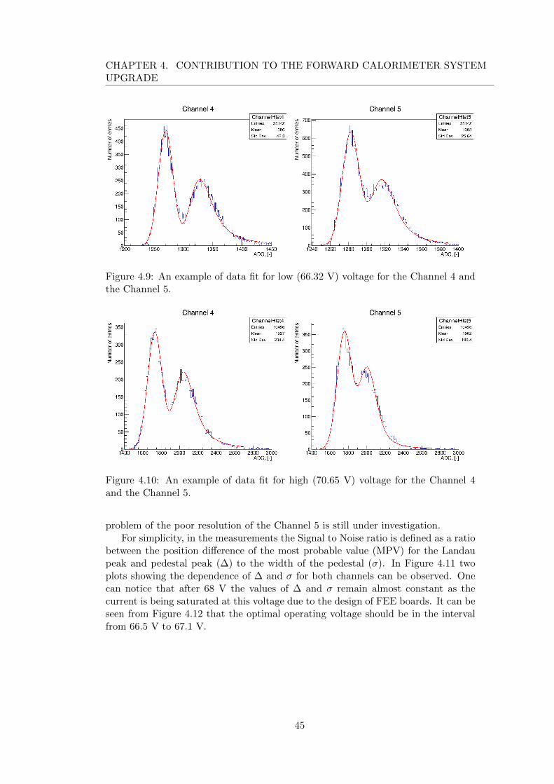
CHAPTER 4. CONTRIBUTION TO THE FORWARD CALORIMETER SYSTEMUPGRADE
Figure 4.9: An example of data fit for low (66.32 V) voltage for the Channel 4 andthe Channel 5.
Figure 4.10: An example of data fit for high (70.65 V) voltage for the Channel 4and the Channel 5.
problem of the poor resolution of the Channel 5 is still under investigation.For simplicity, in the measurements the Signal to Noise ratio is defined as a ratio
between the position difference of the most probable value (MPV) for the Landaupeak and pedestal peak (∆) to the width of the pedestal (σ). In Figure 4.11 twoplots showing the dependence of ∆ and σ for both channels can be observed. Onecan notice that after 68 V the values of ∆ and σ remain almost constant as thecurrent is being saturated at this voltage due to the design of FEE boards. It can beseen from Figure 4.12 that the optimal operating voltage should be in the intervalfrom 66.5 V to 67.1 V.
45
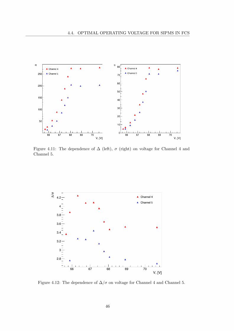
4.4. OPTIMAL OPERATING VOLTAGE FOR SIPMS IN FCS
Figure 4.11: The dependence of ∆ (left), σ (right) on voltage for Channel 4 andChannel 5.
Figure 4.12: The dependence of ∆/σ on voltage for Channel 4 and Channel 5.
46

Chapter 5
Data analysis
5.1 Jet shapes
In order to probe the complimentary aspects of the jet fragmentation and constraindifferent aspects of the theoretical description of jet-medium interactions, differentobservables related to the shapes of jets are studied. In this thesis the attention willbe paid to the two jet shape observables, angularity and momentum dispersion.
The radial moment (alternatively angularity or girth), g, probes the radial dis-tribution of radiation inside a jet. It is defined as
g =∑i∈jet
piT
pT,jet|∆Ri,jet|, (5.1)
where piT represents the momentum of the ith constituent and ∆Ri,jet is the distance
in η × φ plane between the constituent i and the jet axis [49]. η stands for thepseudorapidity (see Appendix A) and φ is the azimuthal angle. This type of shapeis sensitive to the radial energy profile or broadening of the jet. In the collinear limitfor the polar angle (see Appendix A) θ → 0 the radial moment becomes equivalentto jet broadening.
The next observable discussed in this thesis is the momentum dispersion, pTD,given by the equation:
pTD =
√∑i∈jet p
2T,i∑
i∈jet pT,i. (5.2)
This observable measures the second moment of the constituent pT distribution inthe jet and is connected to hardness or softness of the jet fragmentation. In caseof a large number of constituents and softer momentum the pTD tends to 0, whilein the opposite situation, i.e. the small number of constituents carrying the largefraction of momentum, the pTD will be close to 1.
The girth and the momentum dispersion are related to the moments of the soi-disant generalized angularities defined as: λκβ =
∑i(
pT,i
pT,jet)κ(
∆Rjet,i
R )β [50]. For the
number of jet constituents (κ, β) equals to (0, 0), the radial moment g correspondsto (1, 1) and for the square of the momentum dispersion pTD (κ, β) = (2, 0). Onlyfor κ = 1, the shapes are infrared and collinear (IRC) safe.
An example of the measured jet shape distributions for small jets in 0–10%central Pb–Pb collisions at
√sNN = 2.76 TeV for anti-kT charged jets at ALICE
47
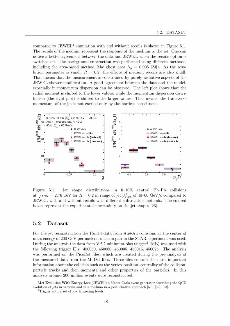
5.2. DATASET
compared to JEWEL1 simulation with and without recoils is shown in Figure 5.1.The recoils of the medium represent the response of the medium to the jet. One cannotice a better agreement between the data and JEWEL when the recoils option isswitched off. The background subtraction was performed using different methods,including the area-based method (the ghost area Ag = 0.005 [23]). As the reso-lution parameter is small, R = 0.2, the effects of medium recoils are also small.That means that the measurement is constrained by purely radiative aspects of theJEWEL shower modification. A good agreement between the data and the model,especially in momentum dispersion can be observed. The left plot shows that theradial moment is shifted to the lower values, while the momentum dispersion distri-bution (the right plot) is shifted to the larger values. That means, the transversemomentum of the jet is not carried only by the hardest constituent.
0 0.05 0.1g
10
20
30
g/d
jets
N d
jets
N1/
= 2.76 TeVNNsPb −10% Pb−0 = 0.2R charged jets, TkAnti-
c 60 GeV/≤ chT,jet
p ≤40
ALICE
ALICE data
JEWEL no recoils
JEWEL recoils (deriv.sub)
JEWEL recoils (const.sub)
ALICE data
JEWEL no recoils
JEWEL recoils (deriv.sub)
JEWEL recoils (const.sub)
ALICE data
JEWEL no recoils
JEWEL recoils (deriv.sub)
JEWEL recoils (const.sub)
0.4 0.6 0.8 1D
Tp
0
2
4
6
DT
p/d
jets
N d
jets
N1/
ALICE data
JEWEL no recoils
JEWEL recoils (deriv.sub)
JEWEL recoils (const.sub)
ALICE data
JEWEL no recoils
JEWEL recoils (deriv.sub)
JEWEL recoils (const.sub)
ALICE data
JEWEL no recoils
JEWEL recoils (deriv.sub)
JEWEL recoils (const.sub)
Figure 5.1: Jet shape distributions in 0–10% central Pb–Pb collisionsat√sNN = 2.76 TeV for R = 0.2 in range of jet pch
T,jet of 40–60 GeV/c compared toJEWEL with and without recoils with different subtraction methods. The coloredboxes represent the experimental uncertainty on the jet shapes [23].
5.2 Dataset
For the jet reconstruction the Run14 data from Au+Au collisions at the center ofmass energy of 200 GeV per nucleon-nucleon pair in the STAR experiment was used.During the analysis the data from VPD minimum-bias trigger2 (MB) was used withthe following trigger IDs: 450050, 450060, 450005, 450015, 450025. The analysiswas performed on the PicoDst files, which are created during the pre-analysis ofthe measured data from the MuDst files. These files contain the most importantinformation about the collision such as the vertex position, centrality of the collision,particle tracks and then momenta and other properties of the particles. In thisanalysis around 200 million events were reconstructed.
1Jet Evolution With Energy Loss (JEWEL) a Monte Carlo event generator describing the QCDevolution of jets in vacuum and in a medium in a perturbative approach [51], [52], [53].
2Trigger with a set of low triggering levels.
48

CHAPTER 5. DATA ANALYSIS
In order to choose only those events or particle tracks that are suitable for theanalysis, different cuts are applied before the jet reconstruction. In this analysis thefollowing event selection and particle tracks were used:
• The position of the primary vertex |zvertex| < 30 cm from the center of thecollision along the beam axis ”z”.
• Pseudorapidity range of tracks: −1.0 < η < 1.0
• Number of points used for the track fit is > 14.
• Number of fit points to maximum number of all possible fit points ratio > 0.52.
• The track momenta are in ptrackT range: 0.2 GeV/c < ptrackT < 30 GeV/c, inorder to exclude the low momentum particles, which cannot provide enoughreconstruction points, and high momentum particles, which can give the largeuncertainties in momentum calculations due to the low bend by the magneticfield.
• The Distance of Closest Approach (DCA) of the track to the primary vertexis less than 1 cm in order to exclude the tracks originating from the secondarydecays.
Figure 5.2: The distance distribution of the primary vertex from the center of theAu+Au collision at energy
√sNN = 200 GeV.
Figure 5.2 shows the distance distribution vz of the primary vertex from thecenter of the collision. As one can see, the distribution is symmetrical. Some of theprimary vertices can be found at the distance larger than 30 cm from the center of
49
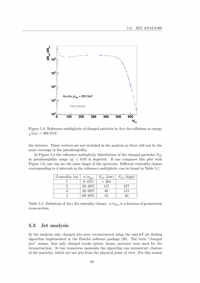
5.3. JET ANALYSIS
Figure 5.3: Reference multiplicity of charged particles in Au+Au collisions at energy√sNN = 200 GeV.
the detector. These vertices are not included in the analysis as there will not be thesame coverage in the pseudorapidity.
In Figure 5.3 the reference multiplicity distribution of the charged particles Nch
in pseudorapidity range |η| < 0.05 is depicted. If one compares this plot withFigure 1.6, one can see the same shape of the spectrum. Different centrality classescorresponding to 4 intervals in the reference multiplicity can be found in Table 5.1.
Centrality bin σ/σgeo Nch (low) Nch (high)
1 0–10% > 364 –
2 20–40% 115 257
3 40–60% 40 115
4 60–80% 10 40
Table 5.1: Definition of Au+Au centrality classes. σ/σgeo is a fraction of geometricalcross-section.
5.3 Jet analysis
In the analysis only charged jets were reconstructed using the anti-kT jet findingalgorithm implemented in the FastJet software package [40]. The term ”chargedjets” means, that only charged tracks (pions, kaons, protons) were used for thereconstruction. At low transverse momenta the algorithm can reconstruct clustersof the particles, which are not jets from the physical point of view. For this reason
50

CHAPTER 5. DATA ANALYSIS
only jets with pchT,jet > 10 GeV/c are used. The analysis was performed in three pch
T,jet
ranges (10–20 GeV/c, 20–30 GeV/c, 30–40 GeV/c) for two resolution parameters:R = 0.2 and R = 0.4.
Figure 5.4 shows the number of constituents for jets with different transversemomenta and different resolution parameters. With the increase of resolution pa-rameter the jet contains more tracks. For this reason the spectra for R = 0.4 areshifted to the right. In the analysis it was also decided to exclude the jets havingonly one constituent, which have no physical interest.
One of the problems arising during the jet reconstruction is large and fluctuatingbackground from the underlying event with fluctuations of the magnitude of the sig-nal. There are different methods which can be used for the background subtraction.One of them is the event-by-event correction, recommended by FastJet authors [40].
From the reconstructed jet transverse momentum, praw,chT,jet one needs to subtract the
median jet energy density ρ multiplied by the jet area A as:
pchT,jet = praw,ch
T,jet − ρ ·A. (5.3)
The jet areaA was calculated using the large amount of the extremely ghost particles,which have been randomly added to the event. The median jet energy density iscalculated as:
ρ = med{piT,jet
Ai} (5.4)
for i running over all jets in the event. For the background calculation the kTalgorithm was used due to a better sensitivity to the soft particles.
Figure 5.5 shows the dependence of the reference multiplicity on the backgrounddensity for R = 0.2 (left) and R = 0.4 (right). In Figure 5.6 the background energydensity distributions for different centrality classes are presented for two resolution
Figure 5.4: Number of constituents in charged jets with R = 0.2 (upper row) and R= 0.4 (bottom row) for different pchT,jet ranges.
51

5.3. JET ANALYSIS
Figure 5.5: Dependence of background density ρ on the charged particle referencemultiplicity (|η| < 0.5) for the resolution parameters of the jet R = 0.2 (left) and R= 0.4 (right).
parameters. It can be seen for the both Figures that the more central is the collision,the more background is present. Table 5.2 contains the mean and RMS values ofthe background density distributions from Figure 5.6. It can be clearly seen fromthe Table as well as from Figure 5.6 that there is almost no dependence of thebackground on the resolution parameter of the jet, but there is, as anticipated, astrong dependence on collision centrality.
Figure 5.6: Background energy density for 4 centrality classes in Au+Au collisions.Left: for jet resolution parameter R = 0.2, right: for jet resolution parameter R =0.4.
In order to correct every constituent of the jet to the background subtractionthe constituent background subtractor described in section 2.5 that is implementedin the FastJet Contribution package was used with the basic settings. The areacovered by the ghost was chosen to be Ag = 0.01, the threshold for the distancesbetween the particle and the ghost was set to ∆Rmax →∞ and the parameter α in
52
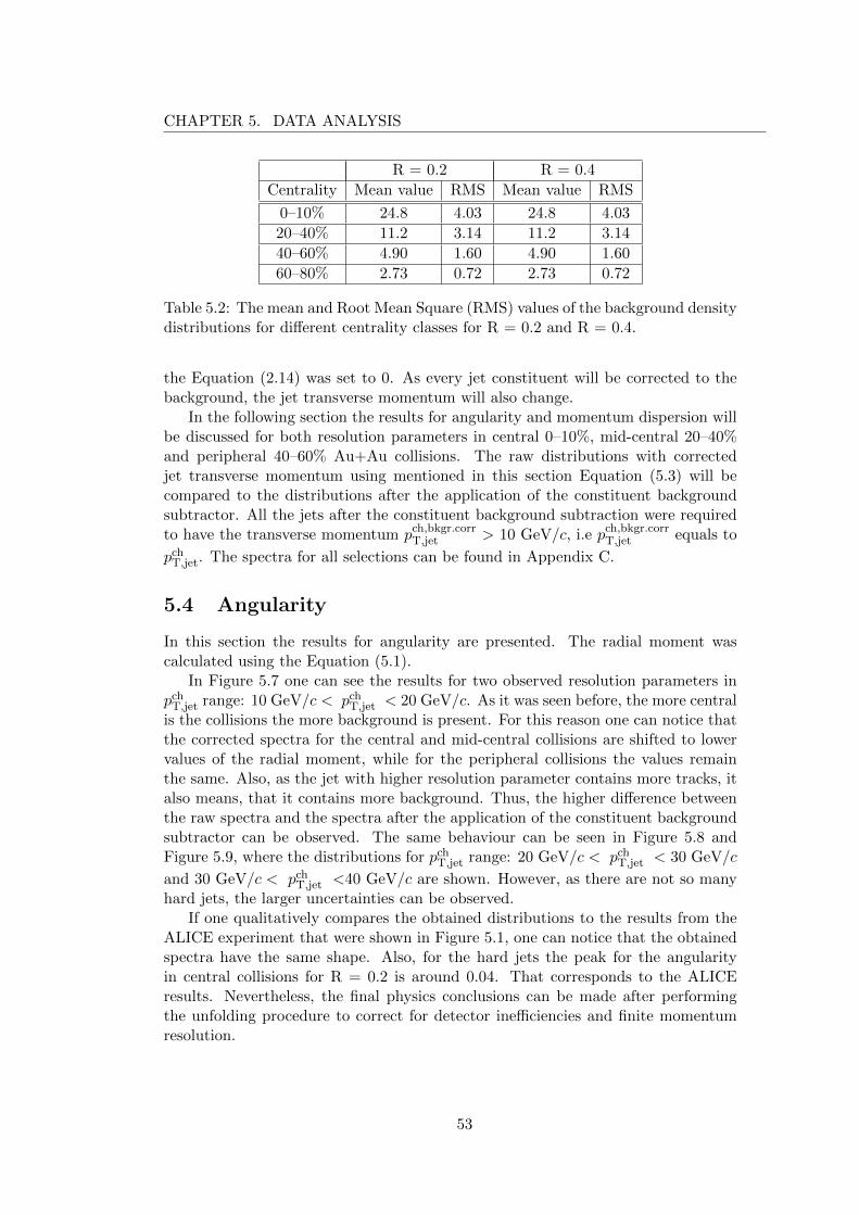
CHAPTER 5. DATA ANALYSIS
R = 0.2 R = 0.4
Centrality Mean value RMS Mean value RMS
0–10% 24.8 4.03 24.8 4.03
20–40% 11.2 3.14 11.2 3.14
40–60% 4.90 1.60 4.90 1.60
60–80% 2.73 0.72 2.73 0.72
Table 5.2: The mean and Root Mean Square (RMS) values of the background densitydistributions for different centrality classes for R = 0.2 and R = 0.4.
the Equation (2.14) was set to 0. As every jet constituent will be corrected to thebackground, the jet transverse momentum will also change.
In the following section the results for angularity and momentum dispersion willbe discussed for both resolution parameters in central 0–10%, mid-central 20–40%and peripheral 40–60% Au+Au collisions. The raw distributions with correctedjet transverse momentum using mentioned in this section Equation (5.3) will becompared to the distributions after the application of the constituent backgroundsubtractor. All the jets after the constituent background subtraction were requiredto have the transverse momentum pch,bkgr.corr
T,jet > 10 GeV/c, i.e pch,bkgr.corrT,jet equals to
pchT,jet. The spectra for all selections can be found in Appendix C.
5.4 Angularity
In this section the results for angularity are presented. The radial moment wascalculated using the Equation (5.1).
In Figure 5.7 one can see the results for two observed resolution parameters inpch
T,jet range: 10 GeV/c < pchT,jet < 20 GeV/c. As it was seen before, the more central
is the collisions the more background is present. For this reason one can notice thatthe corrected spectra for the central and mid-central collisions are shifted to lowervalues of the radial moment, while for the peripheral collisions the values remainthe same. Also, as the jet with higher resolution parameter contains more tracks, italso means, that it contains more background. Thus, the higher difference betweenthe raw spectra and the spectra after the application of the constituent backgroundsubtractor can be observed. The same behaviour can be seen in Figure 5.8 andFigure 5.9, where the distributions for pch
T,jet range: 20 GeV/c < pchT,jet < 30 GeV/c
and 30 GeV/c < pchT,jet <40 GeV/c are shown. However, as there are not so many
hard jets, the larger uncertainties can be observed.If one qualitatively compares the obtained distributions to the results from the
ALICE experiment that were shown in Figure 5.1, one can notice that the obtainedspectra have the same shape. Also, for the hard jets the peak for the angularityin central collisions for R = 0.2 is around 0.04. That corresponds to the ALICEresults. Nevertheless, the final physics conclusions can be made after performingthe unfolding procedure to correct for detector inefficiencies and finite momentumresolution.
53
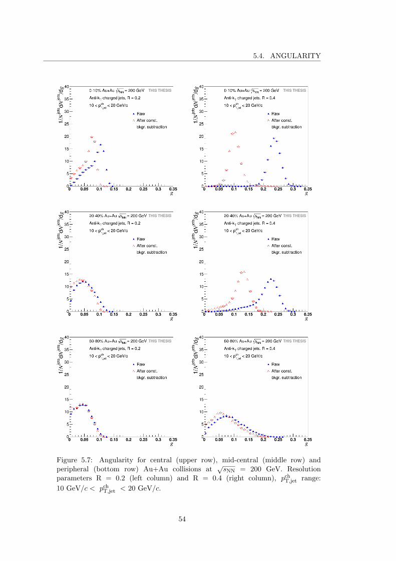
5.4. ANGULARITY
Figure 5.7: Angularity for central (upper row), mid-central (middle row) andperipheral (bottom row) Au+Au collisions at
√sNN = 200 GeV. Resolution
parameters R = 0.2 (left column) and R = 0.4 (right column), pchT,jet range:
10 GeV/c < pchT,jet < 20 GeV/c.
54

CHAPTER 5. DATA ANALYSIS
Figure 5.8: Angularity for central (upper row), mid-central (middle row) andperipheral (bottom row) Au+Au collisions at
√sNN = 200 GeV. Resolution
parameters R = 0.2 (left column) and R = 0.4 (right column), pchT,jet range:
20 GeV/c < pchT,jet < 30 GeV/c.
55

5.4. ANGULARITY
Figure 5.9: Angularity for central (upper row), mid-central (middle row) andperipheral (bottom row) Au+Au collisions at
√sNN = 200 GeV. Resolution
parameters R = 0.2 (left column) and R = 0.4 (right column), pchT,jet range:
30 GeV/c < pchT,jet < 40 GeV/c.
56
CHAPTER 5. DATA ANALYSIS
5.5 Momentum dispersion
This section contains the distributions of momentum dispersion. The observablewas calculated using the Equation (5.2).
In Figure 5.10 the momentum dispersion distributions for central, mid-centraland peripheral Au+Au collisions in pch
T,jet range: 10 GeV/c < pchT,jet < 20 GeV/c
are shown. It can be seen, that the shape of the distribution remains almost thesame for all centralitities. The peak in the last bin in mid-central and peripheralcollisions for R = 0.2 indicates that there are more jets having small number ofconstituents carrying the large fraction of momentum after the application of theconstituent background subtractor. The same peak in the last bin can be observedfor jets having the transverse momentum in 20 GeV/c < pch
T,jet < 30 GeV/c inall centralities for R = 0.2. Momentum dispersion distributions of the jets withtransverse momentum 30 GeV/c < pjetT < 40 GeV/c have only one peak around0.75 and no peak in the last bin, that means that the constituents have approximatelythe same transverse momentum. Also, as for the radial moment results, one can seethe increase of the uncertainties with growing pch
T,jet.
The obtained results for the momentum dispersion in pchT,jet range: 30 GeV/c <
pchT,jet < 40 GeV/c can be qualitatively compared to the results from the ALICE
collaboration. The same shape of the spectra can be observed. However, the max-imum value of the momentum dispersion at ALICE is at 0.55, while the obtaineddistribution for R = 0.2 reaches its maximum at 0.85 for central Au+Au collisionsat RHIC energy. That tells about more even distribution of the transverse momentaof constituents in jets from the ALICE experiment. Again, as for the angularity, thefinal physics conclusions can be made after performing the unfolding procedure tocorrect for detector inefficiencies and finite momentum resolution.
57
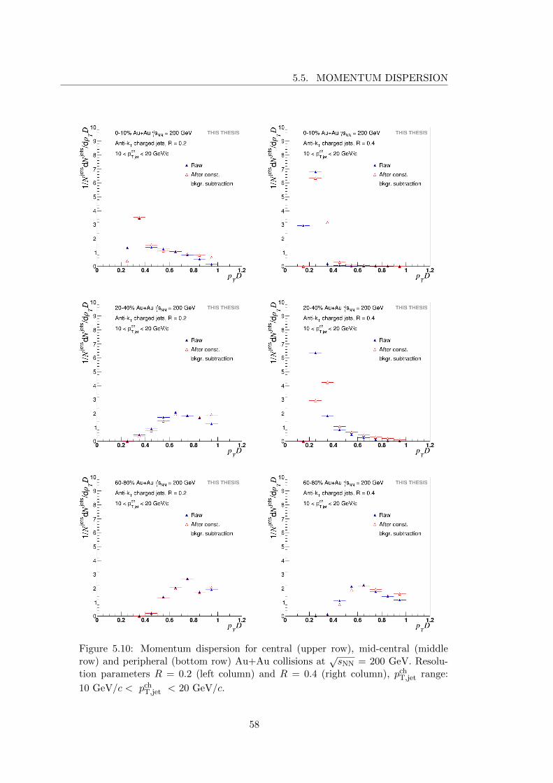
5.5. MOMENTUM DISPERSION
Figure 5.10: Momentum dispersion for central (upper row), mid-central (middlerow) and peripheral (bottom row) Au+Au collisions at
√sNN = 200 GeV. Resolu-
tion parameters R = 0.2 (left column) and R = 0.4 (right column), pchT,jet range:
10 GeV/c < pchT,jet < 20 GeV/c.
58
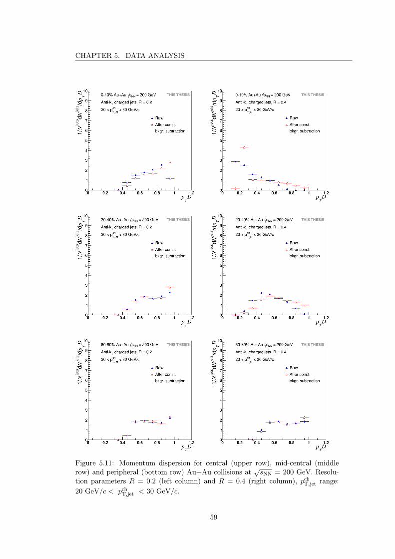
CHAPTER 5. DATA ANALYSIS
Figure 5.11: Momentum dispersion for central (upper row), mid-central (middlerow) and peripheral (bottom row) Au+Au collisions at
√sNN = 200 GeV. Resolu-
tion parameters R = 0.2 (left column) and R = 0.4 (right column), pchT,jet range:
20 GeV/c < pchT,jet < 30 GeV/c.
59

5.5. MOMENTUM DISPERSION
Figure 5.12: Momentum dispersion for central (upper row), mid-central (middlerow) and peripheral (bottom row) Au+Au collisions at
√sNN = 200 GeV. Reso-
lution parameters R = 0.2 (left column) and R = 0.4 (right column), pjetT range:
30 GeV/c < pjetT < 40 GeV/c.
60

Chapter 6
Summary
This thesis is devoted to study of jet shape observables in Au+Au collisions in theSTAR experiment as well as to my service work at Brookhaven National Laboratory.
As a part of the one-month Service work at BNL I had an opportunity to par-ticipate in the Forward Calorimeter System (FCS) upgrade. In this period I havehelped in different projects for Hadronic and Electromagnetic Calorimeters, thatare described in Chapter 4. The 600 tiles have been polished and painted and arenow ready for the installation in the HCal. Also, the characteristics of the SiliconPhotomultipliers (SiPMs) provided by Hamamatsu have been checked. As a result,it was decided to order the SiPMs with the variation of ±20 mV of the operatingvoltage within a tray. The last task was the data analysis from the cosmic muonsetup in order to get the optimal operating voltage for the SiPMs that will be usedin FCS. The setup was built using the preshower detector that was irradiated inRun17. During the analysis it was found that the optimal operating voltage shouldbe in the interval from 66.5 V to 67.1 V. The analysis is still ongoing in order toeliminate various problems with the setup and achieve more reliable results.
The main part of this thesis is dedicated to study of two jet shape observables:radial moment and momentum dispersion in Au+Au collisions at
√sNN = 200 GeV
at the STAR experiment. The charged jets were reconstructed using the anti-kTalgorithm and the jet shape observables were calculated in three jet pch
T,jet ranges (10–20 GeV/c, 20–30 GeV/c, 30–40 GeV/c) for two resolution parameters: R = 0.2 andR = 0.4. In order to get physics interpretable results the background was subtractedusing the constituent background subtractor implemented in the FastJet software.For the subtraction the basic settings were used. All the jet shape distributions havebeen calculated for different centrality classes: 0–10%, 20–40%, 40–60%, 60–80%.The jets having only one constituent, were excluded from the analysis. The shiftof the angularity spectra to the lower values indicates of that after the backgroundsubtraction the jets become softer, i.e. more constituents carry small fraction ofthe momentum. The data also suggests to make the same conclusion based on thefact that momentum dispersion distributions are shifted closer to 1. The differencein the shifts of the peaks for angularity for different resolution parameters after theapplication of the constituent background subtractor is due to that wider jets containmore background. The obtained distributions for radial moment and momentumdispersion have qualitatively the same shape as the distributions from the ALICEcollaboration.
61

Nevertheless, the performed correction by using the constituent background sub-tractor is only a first step of the all corrections that are needed to be made. In futureanalysis it is planed to correct the jet shape observables for detector effects via two-dimensional unfolding described briefly in Chapter 2 to get final physics results,which can be then compared with model calculations.
62
Appendix A
Basic kinematic observables
In order to describe the properties of particles created in nuclear-nuclear collisions,it is good to define some variables accounting for relativistic effects.
A.1 Transverse momentum
The importance of the transverse momentum arises because momentum along thebeamline may just be left over from the beam particles, while the transverse momen-tum is always associated with whatever physics happened at the collision vertex.
The transverse momentum pT is defined as
pT =√p2x + p2
y, (A.1)
where the px and py are the components of the three-momentum −→p = (px, py, pz),the last component, pz, is the component of the momentum along the beam axis(longitudinal momentum pL).
A.2 Rapidity and pseudorapidity
The rapidity, y, is a measure of velocity. It is defined as
y =1
2ln
(E + pLE − pL
), (A.2)
where pL is the longitudinal momentum and E is the energy of the particle. Therapidity is related to the angle between the XY plane and the direction of emissionof a product of the collision.
As the rapidity can be hard to measure for highly relativistic particles, the pseu-dorapidity, η, is usually used in experimental particle physics instead of rapidity y.The pseudorapidity is determined by the following equation:
η = − ln
(tan
θ
2
), (A.3)
where θ is the angle between the particle three-momentum −→p and the positivedirection of the beam axis. In comparison to rapidity, pseudorapidity depends onlyon the polar angle of the particle’s trajectory, and not on the energy of the particle.The dependence of the pseudorapidity on the polar angle is shown in the Figure A.1.
63
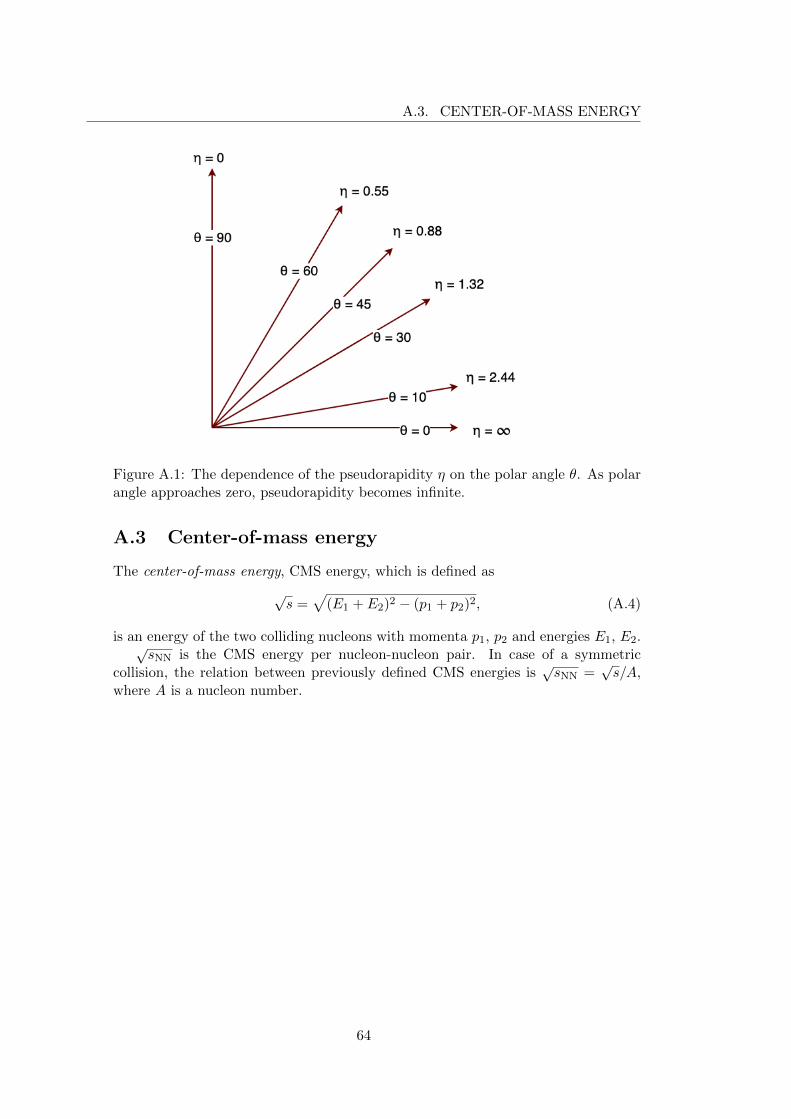
A.3. CENTER-OF-MASS ENERGY
Figure A.1: The dependence of the pseudorapidity η on the polar angle θ. As polarangle approaches zero, pseudorapidity becomes infinite.
A.3 Center-of-mass energy
The center-of-mass energy, CMS energy, which is defined as
√s =
√(E1 + E2)2 − (p1 + p2)2, (A.4)
is an energy of the two colliding nucleons with momenta p1, p2 and energies E1, E2.√sNN is the CMS energy per nucleon-nucleon pair. In case of a symmetric
collision, the relation between previously defined CMS energies is√sNN =
√s/A,
where A is a nucleon number.
64
Appendix B
Bad run list
Following runs have been removed from the analysis: 15077043, 15077057, 15077063,15077067, 15077070, 15077080, 15078003, 15078005, 15078006, 15078017, 15078021,15078073, 15078075, 15078103, 15078108, 15078111, 15079001, 15079002, 15079013,15079016, 15079017, 15079019, 15079022, 15079024, 15079025, 15079026, 15079027,15079042, 15079047, 15079056, 15079057, 15079059, 15079060, 15079061, 15080002,15080003, 15080004, 15080005, 15080006, 15080007, 15080011, 15080012, 15080013,15080014, 15080016, 15080036, 15080037, 15080041, 15080044, 15080045, 15080053,15080057, 15080058, 15080059, 15080061, 15081001, 15081006, 15081007, 15081023,15081025, 15081028, 15081036, 15081038, 15081041, 15081042, 15081044, 15082008,15082016, 15082023, 15082024, 15082025, 15082028, 15082030, 15082059, 15082060,15082073, 15082075, 15083003, 15083005, 15083014, 15083021, 15083023, 15083024,15083027, 15083028, 15084002, 15084008, 15084011, 15084022, 15084027, 15084029,15084030, 15084036, 15084037, 15097023, 15097032, 15097034, 15097055, 15097059,15097061, 15097063, 15098010, 15098039, 15098040, 15098067, 15100100, 15100101,15100102, 15100103, 15102021, 15102024, 15103020, 15104016, 15104018, 15105008,15106009, 15107077, 15108069, 15109013, 15110032, 15110038, 15111013, 15119021,15119026, 15119027, 15119028, 15119042, 15119056, 15120011, 15121062, 15124004,15126021, 15126040, 15126060, 15130032, 15130035, 15142054, 15144018, 15145015,15145016, 15149062, 15150057, 15151004, 15151005, 15151042, 15153050, 15154013,15157020, 15157022, 15157052, 15157058, 15158024, 15158028, 15158031, 15158032,15158033, 15158035, 15158070, 15159021, 15160006, 15161003, 15161004, 15161012,15161014, 15161053, 15161065, 15162013, 15162025, 15162026, 15162042, 15162047,15163004, 15163005, 15163022, 15163054, 15164003, 15164049, 15164066, 15165027,15165031, 15166023, 15166028.
65

66
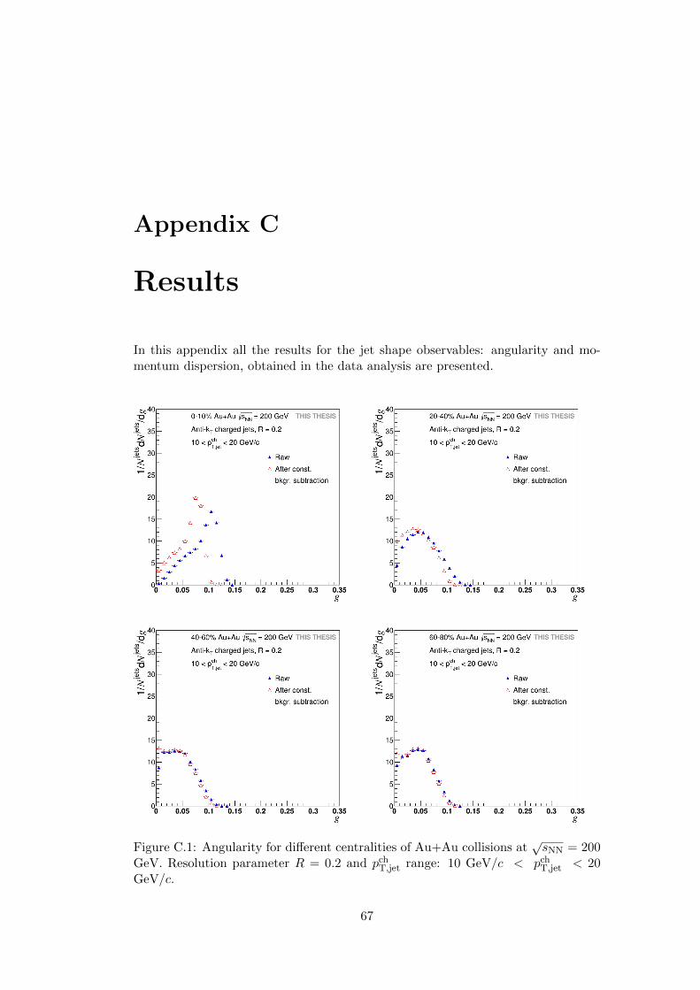
Appendix C
Results
In this appendix all the results for the jet shape observables: angularity and mo-mentum dispersion, obtained in the data analysis are presented.
Figure C.1: Angularity for different centralities of Au+Au collisions at√sNN = 200
GeV. Resolution parameter R = 0.2 and pchT,jet range: 10 GeV/c < pch
T,jet < 20GeV/c.
67

Figure C.2: Angularity for different centralities of Au+Au collisions at√sNN
= 200 GeV. Resolution parameter of the jet R = 0.4 and pchT,jet range:
10 GeV/c < pchT,jet < 20 GeV/c.
68
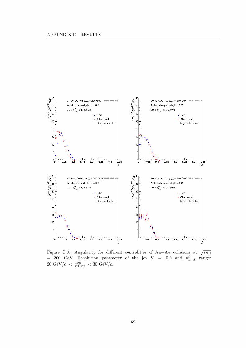
APPENDIX C. RESULTS
Figure C.3: Angularity for different centralities of Au+Au collisions at√sNN
= 200 GeV. Resolution parameter of the jet R = 0.2 and pchT,jet range:
20 GeV/c < pchT,jet < 30 GeV/c.
69

Figure C.4: Angularity for different centralities of Au+Au collisions at√sNN
= 200 GeV. Resolution parameter of the jet R = 0.4 and pchT,jet range:
20 GeV/c < pchT,jet < 30 GeV/c.
70
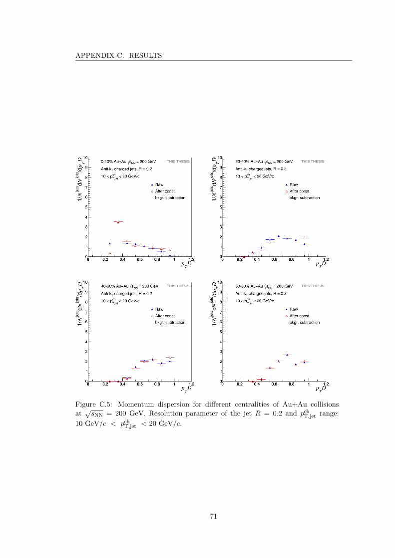
APPENDIX C. RESULTS
Figure C.5: Momentum dispersion for different centralities of Au+Au collisionsat√sNN = 200 GeV. Resolution parameter of the jet R = 0.2 and pch
T,jet range:
10 GeV/c < pchT,jet < 20 GeV/c.
71

Figure C.6: Momentum dispersion for different centralities of Au+Au collisionsat√sNN = 200 GeV. Resolution parameter of the jet R = 0.4 and pch
T,jet range:
10 GeV/c < pchT,jet < 20 GeV/c.
72
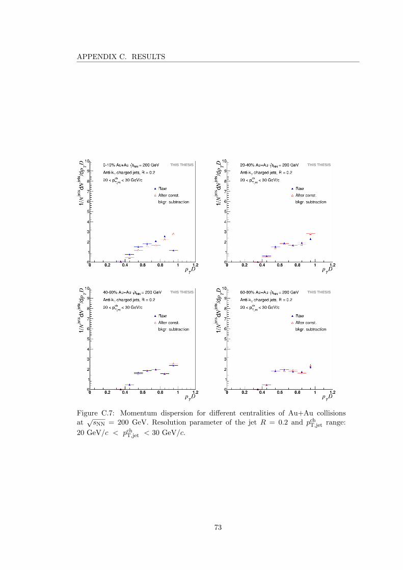
APPENDIX C. RESULTS
Figure C.7: Momentum dispersion for different centralities of Au+Au collisionsat√sNN = 200 GeV. Resolution parameter of the jet R = 0.2 and pch
T,jet range:
20 GeV/c < pchT,jet < 30 GeV/c.
73

Figure C.8: Momentum dispersion for different centralities of Au+Au collisionsat√sNN = 200 GeV. Resolution parameter of the jet R = 0.4 and pch
T,jet range:
20 GeV/c < pchT,jet < 30 GeV/c.
74
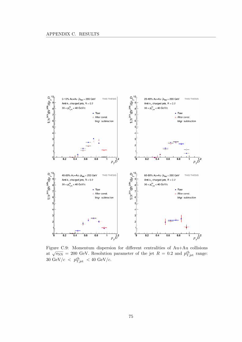
APPENDIX C. RESULTS
Figure C.9: Momentum dispersion for different centralities of Au+Au collisionsat√sNN = 200 GeV. Resolution parameter of the jet R = 0.2 and pch
T,jet range:
30 GeV/c < pchT,jet < 40 GeV/c.
75

Figure C.10: Momentum dispersion for different centralities of Au+Au collisionsat√sNN = 200 GeV. Resolution parameter of the jet R = 0.4 and pch
T,jet range:
30 GeV/c < pchT,jet < 40 GeV/c.
76
Bibliography
[1] Brookhaven National Laboratory. RHIC. https://www.bnl.gov/rhic/. [on-line 5.5.2018].
[2] R. Stock. Relativistic Nucleus-Nucleus Collisions and the QCD Matter PhaseDiagram. [arXiv 0807.1610].
[3] S. Sarkar et al. The Physics of the Quark-Gluon Plasma: Introductory Lectures.Springer Berlin Heidelberg, 2009. ISBN 978-3-642-02286-9.
[4] M. L. Miller, K. Reygers, S. J. Sanders, P. Steinberg. Glauber modeling in highenergy nuclear collisions, Ann. Rev. Nucl. Part. Sci., 57:205-243, 2007.
[5] F. Tanedo. The picture is taken from:. http://www.quantumdiaries.org/
wp-content/uploads/2011/04/clustering.png. [online 1.12.2018].
[6] Heavy flavor. https://drupal.star.bnl.gov/STAR/pwg/heavy-flavor. [on-line 10.10.2019].
[7] CMS collaboration. Charged-particle nuclear modification factors in PbPb andpPb collisions at
√sN N = 5.02 TeV, JHEP 04(039)2017.
[8] STAR collaboartion. Centrality and transverse momentum dependence of D0-meson production at mid-rapidity in Au+Au collisions at
√sNN = 200 GeV,
Phys. Rev. C 99, 034908 (2019).
[9] M. Aaboud et al. Measurement of the nuclear modification factor for inclusivejets in Pb+Pb collisions at
√sNN = 5.02 TeV with the ATLAS detector, Phys.
Lett. B790(2019)108-128.
[10] CMS Collaboration. Measurement of Jet Nuclear Modification Factor in PbPbCollisions at
√sNN = 5.02 TeV with CMS, 2019. http://cds.cern.ch/
record/2698506.
[11] S. Acharya et al. ALICE. Measurements of inclusive jet spectra in pp andcentral Pb-Pb collisions at
√sNN = 5.02 TeV.
[12] Jan Rusnak. Jet Reconstruction in Au+Au collisions at RHIC. https://
drupal.star.bnl.gov/STAR/theses/phd/janrusnak. [online 05.12.2019].
[13] G. C. Blazey et. al. Run II jet physics, [hep-ex/0005012].
[14] G. Soyez M. Cacciari, G. P. Salam. The Anti-k(t) jet clustering algorithm.JHEP, 04:063, 2008.
77

BIBLIOGRAPHY
[15] M. Cacciari, G. P. Salam. Dispelling the N3 myth for the kt jet-finder. Phys.Lett.,B641:57-61, 2006.
[16] Nuclear Science and Technology. https://nsww.org/projects/bnl/star/
trigger-system.php. [online 13.8.2018].
[17] M. Anderson, J. Berkovitz, W. Betts et.al. The STAR Time Projection Cham-ber: A Unique Tool for Studying High Multiplicity Events at RHIC, [arXiv:nucl-ex/0301015v1], 2003.
[18] J. Adam et al. Centrality and transverse momentum dependence of D0 -mesonproduction at mid-rapidity in Au+Au collisions at
√sNN = 200 GeV, Phys.
Rev., C99(3):034908,2019.
[19] M. Beddo, E. Bielick, T. Fornek et.al. The STAR Barrel ElectromagneticCalorimeter. https://www.star.bnl.gov/public/tpc/NimPapers/emc/emc_
nim.pdf, 2002.
[20] W. J. Llope et al. STAR. The STAR Vertex Position Detector, Nucl. Instrum.Meth., A759(2014)23-28 .
[21] The STAR TOF collaboration. Proposal for a large area Time Of Flightsystem for STAR. https://www.star.bnl.gov/public/tof/publications/
TOF_20040524.pdf, 2004.
[22] STAR Collaboration. The star forward calorimeter system and forward trackingsystem, 2018.
[23] S. Acharya et al. ALICE. Medium modification of the shape of small-radiusjets in central Pb-Pb collisions at
√sNN = 2.76 TeV, JHEP 10:139, 2018.
[24] F. Karsch. Lectures on quark matter. Proceedings, 40. International Universi-tatswochen for theoretical physics, 40th Winter School, IUKT 40, Lect. NotesPhys.583, 209 (2002).
[25] Z. Fodor, S. D. Katz. High Energy Physics - Lattice Critical point of QCD atfinite T and µ, lattice results for physical quark masses, JHEP 04, 050 (2004).
[26] J.D. Bjorken. In Current Induced Reactions, Lecture Notes in Physics vol.56.New York: Springer, p.93, 1976.
[27] L.D Landau. Izv. Akad. Nauk SSSR 17, 51; reprinted (1965) in CollectivePapers of L. D. Landau”, ed. D. T. ter Haar New York: Gordon & Breach, p.596, 1953.
[28] K. Yagi, T. Hatsuda, Y. Miake. Quark-Gluon Plasma. Cambridge UniversityPress, 2005.
[29] R. J. Glauber. Lectures on Theoretical physics”, vol. 1. New York: Interscience,p. 315, 1959.
[30] J. Chyla. Quarks, partons and Quantum Chromodynamics. https://www.fzu.cz/~chyla/lectures/text.pdf. [online 12.06.2019].
78
BIBLIOGRAPHY
[31] Particle Data Group. The Review of Particle Physics (2019).
[32] A. Grozin. Heavy Quark Effective Theory, Springer, Berlin, Heidelberg, 2004.
[33] J. Adams et al. Transverse momentum and collision energy dependence ofhigh pT hadron suppression in Au+Au collisions at ultrarelativistic energiesPhys.Rev.Lett. 91, 172302.
[34] S. Adler et al. Suppressed π0 Production at Large Transverse Momentum inCentral Au+Au Collisions at
√sNN = 200 GeV Phys.Rev.Lett. 91, 072301.
[35] B. Back et al. (PHOBOS). Pseudorapidity dependence of charged hadron trans-verse momentum spectra in d+Au collisions at
√sNN ) = 200 GeV Phys.Rev.
C70, 061901, (2004).
[36] Yu. L. Dokshitzer et al. Heavy quark colorimetry of QCD matter,Phys.Lett.B519:199- 206,2001.
[37] G. P. Salam. Towards Jetography, [arXiv: 0906.1140], Eur. Phys. J. C67:637–686, 2010.
[38] G. Soyez M. Cacciari, G. P. Salam. The Catchment Area of Jets, JHEP 04:005,2008.
[39] G. Salam, G. Soyez. The SISCone Jet Algorithm. https://siscone.hepforge.org/.
[40] M. Cacciari, G. P. Salam, G. Soyez. FastJet user manual. [arXiv: 1111.6097].
[41] G. L. Dirichlet, J. Reine. Math.40 (1850) 209.
[42] M. Cacciari, G. P. Salam. Pileup subtraction using jet areas, Phys. Lett. B659(2008) 119.
[43] G. D’Agostini. Improved iterative Bayesian unfolding, 2010, arXiv:1010.0632.
[44] G. D’Agostini. A multidimensional unfolding method based on Bayes’ theorem,Meth. in Phys. Res. A362 (487) 1995.
[45] A. Hocker, V. Kartvelishvili. SVD approach to data unfolding, Nucl. Instrum.Meth.(469-481)1996.
[46] B. A. Schwartz C. Grupen. Particle Detectors, 2nd edition, Cambridge Univer-sity Press, 2009.
[47] The RHIC Zero Degree Calorimeters. https://www.phenix.bnl.gov/
~swhite/zcal/index.html. [online 13.8.2018].
[48] C. Chasman, D. Beavis, R. Debbe et.al. A Heavy Flavor Tracker for STAR.http://rnc.lbl.gov/~wieman/hft_final_submission_version.pdf. [on-line 6.5.2018].
[49] L. Cunqueiro. Jet shapes in pp and Pb–Pb collisions at ALICE. Nucl. Phys.,A956:593–596, 2016.
79
BIBLIOGRAPHY
[50] W. J. Waalewijn A. J. Larkoski, J. Thaler. Gaining (Mutual) Information aboutQuark/Gluon Discrimination, JHEP 11:129, 2014.
[51] K. C. Zapp. JEWEL 2.0.0: Directions for use. Eur. Phys. J., C74(2):2762,2014.
[52] K. C. Zapp. Geometrical aspects of jet quenching in JEWEL, Phys. Lett.,B735:157–163, 2014.
[53] J. Rathsman J. Stachel U.A. Wiedemann K. Zapp, G. Ingelman. A MonteCarlo Model for ’Jet Quenching’, Eur. Phys. J. C60:617-632, 2009.
80