cyber-attack drone payload development and geolocation via
TRANSCRIPT

Air Force Institute of Technology Air Force Institute of Technology
AFIT Scholar AFIT Scholar
Theses and Dissertations Student Graduate Works
3-22-2019
Cyber-Attack Drone Payload Development and Geolocation via Cyber-Attack Drone Payload Development and Geolocation via
Directional Antennae Directional Antennae
Clint M. Bramlette
Follow this and additional works at: https://scholar.afit.edu/etd
Part of the Information Security Commons, and the Navigation, Guidance, Control and Dynamics
Commons
Recommended Citation Recommended Citation Bramlette, Clint M., "Cyber-Attack Drone Payload Development and Geolocation via Directional Antennae" (2019). Theses and Dissertations. 2247. https://scholar.afit.edu/etd/2247
This Thesis is brought to you for free and open access by the Student Graduate Works at AFIT Scholar. It has been accepted for inclusion in Theses and Dissertations by an authorized administrator of AFIT Scholar. For more information, please contact [email protected].
CYBER-ATTACK DRONE PAYLOAD DEVELOPMENT
AND
GEOLOCATION VIA DIRECTIONAL ANTENNAE
THESIS
Clint M. Bramlette, Captain, USAF
AFIT-ENG-MS-19-M-012
DEPARTMENT OF THE AIR FORCE AIR UNIVERSITY
AIR FORCE INSTITUTE OF TECHNOLOGY
Wright-Patterson Air Force Base, Ohio
DISTRIBUTION STATEMENT A.
APPROVED FOR PUBLIC RELEASE; DISTRIBUTION UNLIMITED.

The views expressed in this thesis are those of the author and do not reflect the official
policy or position of the United States Air Force, Department of Defense, or the United
States Government. This material is declared a work of the U.S. Government and is not
subject to copyright protection in the United States.

AFIT-ENG-MS-19-M-012
CYBER-ATTACK DRONE PAYLOAD DEVELOPMENT
AND
WI-FI GEOLOCATION VIA DIRECTIONAL ANTENNAE
THESIS
Presented to the Faculty
Department of Electrical and Computer Engineering
Graduate School of Engineering and Management
Air Force Institute of Technology
Air University
Air Education and Training Command
In Partial Fulfillment of the Requirements for the
Degree of Master of Science in Cyberspace Operations
Clint M. Bramlette, B.S. Wireless Engineering
Captain, USAF
March 2019
DISTRIBUTION STATEMENT A.
APPROVED FOR PUBLIC RELEASE; DISTRIBUTION UNLIMITED.

AFIT-ENG-MS-19-M-012
CYBER-ATTACK DRONE PAYLOAD DEVELOPMENT
AND
WI-FI GEOLOCATION VIA DIRECTIONAL ANTENNAE
Clint M. Bramlette, B.S. Wireless Engineering
Captain, USAF
Committee Membership:
Barry E. Mullins, Ph.D., P.E.
Chair
Timothy H. Lacey, Ph.D., CISSP
Member
Robert F. Mills, Ph.D.
Member

iv
AFIT-ENG-MS-19-M-012
Abstract
The increasing capabilities of commercial drones have led to blossoming drone
usage in private sector industries ranging from agriculture to mining to cinema.
Commercial drones have made amazing improvements in flight time, flight distance, and
payload weight. These same features also offer a unique and unprecedented commodity
for wireless hackers—the ability to gain ‘physical’ proximity to a target without personally
having to be anywhere near it. This capability is called Remote Physical Proximity
(RPP).
By their nature, wireless devices are largely susceptible to sniffing and injection
attacks, but only if the attacker can interact with the device via physical proximity. A
properly outfitted drone can increase the attack surface with RPP (adding a range of over
7 km using off-the-shelf drones), allowing full interactivity with wireless targets while the
attacker can remain distant and hidden. Combined with the novel approach of using a
directional antenna, these drones could also provide the means to collect targeted
geolocation information of wireless devices from long distances passively, which is of
significant value from an offensive cyberwarfare standpoint.
This research develops skypie, a software and hardware framework designed for
performing remote, directional drone-based collections. The prototype is inexpensive,
lightweight, and totally independent of drone architecture, meaning it can be strapped to
most medium to large commercial drones. The prototype effectively simulates the type of

v
device that could be built by a motivated threat actor, and the development process
evaluates strengths and shortcoming posed by these devices.
This research also experimentally evaluates the ability of a drone-based attack
system to track its targets by passively sniffing Wi-Fi signals from distances of 300 and
600 meters using a directional antenna. Additionally, it identifies collection techniques and
processing algorithms for minimizing geolocation errors.
Results show geolocation via 802.11 emissions (Wi-Fi) using a portable directional
antenna is possible, but difficult to achieve the accuracy that GPS delivers (errors less
than 5 m with 95% confidence). This research shows that geolocation predictions of a
target cell phone acting as a Wi-Fi access point in a field from 300 m away is accurate
within 70.1 m from 300 m away and within 76 meters from 600 m away. Three of the
four main tests exceed the hypothesized geolocation error of 15% of the sensor-to-target
distance, with tests 300 m away averaging 25.5% and tests 600 m away averaging at 34%.
Improvements in bearing prediction are needed to reduce error to more tolerable
quantities, and this thesis discusses several recommendations to do so.
This research ultimately assists in developing operational drone-borne cyber-attack
and reconnaissance capabilities, identifying limitations, and enlightening the public of
countermeasures to mitigate the privacy threats posed by the inevitable rise of the cyber-
attack drone.
vi
Acknowledgments
Dedicated to the love of my life, bagels.
I would like to express my sincere gratitude to Dr. Mullins for his support, advice,
knowledge, and the opportunity to pursue the coolest research project at AFIT. Your
enthusiasm and skillset are inspiring.
Thank you to Dr. Lacey, Dr. Mills, and the rest of the AFIT faculty for their support,
expertise, and guidance.
Shoutout to K-Dawg for designing and printing the 3D files.
Thank you to my parents, who encouraged me to go to school.
Clint M. Bramlette

vii
Table of Contents
Page
1. Introduction ............................................................................................................. 1
1.1 Overview and Background ............................................................................... 1
1.2 Research Goals ................................................................................................ 2
1.3 Problem Statement .......................................................................................... 2
1.4 Hypotheses ...................................................................................................... 3
1.5 Approach ......................................................................................................... 4
1.6 Assumptions and Limitations .......................................................................... 4
1.7 Contributions .................................................................................................. 5
1.8 Thesis Overview .............................................................................................. 6
2. Background and Related Research ........................................................................... 7
2.1 The Scene ........................................................................................................ 7
2.2 Overview ......................................................................................................... 8
2.3 Drones ............................................................................................................. 9
2.3.1 Terminology .............................................................................................. 9
2.3.2 Military Drones ....................................................................................... 10
2.3.3 Commercial Drones ................................................................................. 12
2.3.4 Academic Interest ................................................................................... 14
2.4 Wireless Technologies .................................................................................... 15
2.4.1 Wi-Fi ...................................................................................................... 15
2.5 Wi-Fi Security Protocols & Attacks .............................................................. 15
2.5.1 Open Configuration ................................................................................. 16
2.5.2 WEP ....................................................................................................... 17
2.5.3 WPA ....................................................................................................... 18
2.5.4 WPA2 ..................................................................................................... 18
2.5.5 WPA and WPA2 Brute Force Attacks ................................................... 20
2.5.6 WPA3 ..................................................................................................... 22
2.6 IoT ................................................................................................................ 22
2.7 Cybersecurity and Information Warfare ........................................................ 23
2.8 Related Research ........................................................................................... 25
2.8.1 Wireless-Sensing Drones .......................................................................... 25
2.8.2 Identification from Location .................................................................... 27
2.8.3 Proof of Concept: Drones That Can Hack ............................................... 27
2.8.4 Directional Antenna ................................................................................ 30
2.8.5 Data Leakage .......................................................................................... 30

viii
2.9 Background Summary ................................................................................... 31
3. Prototype Design ................................................................................................... 32
3.1 Overview ....................................................................................................... 32
3.2 System Summary........................................................................................... 36
3.2.1 localizer Summary ............................................................................ 36
3.2.2 skypie System Summary ...................................................................... 38
3.3 Design Goals ................................................................................................. 42
3.3.1 localizer Design Goals ...................................................................... 42
3.3.2 skypie Design Goals ............................................................................. 42
3.4 skypie Hardware Design ............................................................................ 44
3.5 skypie Software .......................................................................................... 50
3.5.1 Design Paradigm ..................................................................................... 50
3.5.2 skypie Package .................................................................................... 52
3.5.3 skyport Package .................................................................................. 57
3.5.4 shared Package ..................................................................................... 69
3.5.5 Microcontroller ........................................................................................ 70
3.6 Analysis Algorithms ...................................................................................... 71
3.6.1 Bearing Prediction and Geolocation Algorithm 1 (BPGA1) .................... 72
3.6.2 Geolocation Prediction Averaging Algorithm 1 (GPAA1) ....................... 74
3.7 Design Summary ........................................................................................... 76
4. Methodology .......................................................................................................... 77
4.1 Overview and Objectives ............................................................................... 77
4.2 System Under Test ........................................................................................ 78
4.3 Factors .......................................................................................................... 78
4.4 Metrics .......................................................................................................... 81
4.5 Constant Variables ........................................................................................ 82
4.6 Uncontrolled Variables .................................................................................. 85
4.7 Experimental Design ..................................................................................... 86
4.7.1 Geolocation Experiment: localizer .................................................... 86
4.7.2 Bearing Variance Experiment: localizer ........................................... 88
4.7.3 Geolocation Experiment: skypie .......................................................... 89
4.8 Summary ....................................................................................................... 90
5. Results ................................................................................................................... 91
5.1 Overview ....................................................................................................... 91
5.2 Geolocation Experiment: localizer ........................................................... 91
5.2.1 Bearing Prediction .................................................................................. 92

ix
5.2.2 Geolocation Prediction ............................................................................ 98
5.2.3 Experiment Summary ........................................................................... 113
5.3 Geolocation Experiment: skypie ................................................................ 122
5.4 skypie Framework Developments Results .................................................. 125
5.4.1 Hardware Design Decisions and Rationale ............................................ 125
5.4.2 skypie Framework Functionality ....................................................... 127
6. Conclusion and Future Work ................................................................................ 129
6.1 Overview ...................................................................................................... 129
6.2 Research Conclusions ................................................................................... 129
6.2.1 Geolocation via Radiolocation Conclusions ........................................... 129
6.2.2 BPGA1 and GPAA1 Conclusions ......................................................... 131
6.3 Research Significance and Synthesis ............................................................. 131
6.4 Countermeasures .......................................................................................... 133
6.5 Future Work ................................................................................................ 134
Appendix A. Supplemental skypie Design Resources……………………………………………..139
Bibliography ................................................................................................................. 147

x
List of Figures
Figure Page
1. Exploded Venn-diagram highlighting the intersection of MAUVs, Wi-Fi, and
CNA/CNE, which is the focus of this research .......................................................... 9
2. Number of UAV papers published from the top eight journals/conferences [23] ....... 14
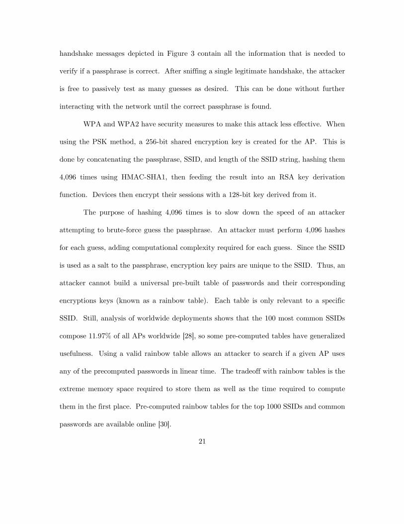
3. WPA2 four-way handshake. On the left is the Station (STA) and the right is the Access
Point (AP) .............................................................................................................. 20
4. DJI Phantom 2 Vision+ with an omnidirectional antenna payload (above) and
accompanying component schematic (below) [38] .................................................... 29
5. localizer prototype ............................................................................................... 33
6. skypie sensor prototype .......................................................................................... 34
7. Hardware components presented in an ‘exploded’ fashion for ease of viewing ............ 35
8. localizer prototype schematic [41] ........................................................................ 37
9. skypie/skyport system design .............................................................................. 41
10. skypie payload hardware schematic ...................................................................... 44
11. 3D printed structure components ............................................................................. 49
12. Structure components assembled on prototype ....................................................... 49
13: skypie control flow diagram .................................................................................. 53
14. ‘SKY’ telemetry sentence ......................................................................................... 55
15. Sensor App User Interface ....................................................................................... 59
16. In-app sensor selection dropdown (left) and the skyport/database/sensors/
directory (right), showing that database is saved as a simple folder scheme............ 60
17. Geolocation history can be viewed in the ‘Telemetry Tab.’ Hovering over each
coordinate shows a box that describes the exact time and location of that point. Dots
are color coded chronologically. The last recorded coordinates and bearing are printed
at the top of the tab. .............................................................................................. 61

xi
18. View history of compass heading ‘Heading Line Draw Density’ value slider. Each
purple ray extends from a coordinate in time and indicates which way the sensor was
facing. In this example, the antenna is mounted to a bicycle doing a half-circle. ... 63
19. ‘Log’ tab enables user to view remote sensor’s skypie logs. ................................... 64
20. Using the ‘Console’ tab to execute ‘ifconfig’ and ‘whoami’ commands. .................... 64
21. ‘Sensor’ settings tab, which allows the attacker to make configuration changes.
Changes are posted by clicking the ‘Submit’ button. .............................................. 65
22. ‘Wi-Fi’ settings tab. Note Mirror mode and Bluetooth mode are stubs that are not
implemented in the scope of this research (discussed in Chapter 6). ....................... 66
23. skyport Analysis App UI ...................................................................................... 68
24. Available targets from each selected sensor are populated in a dropdown in the Analysis
App. One, multiple, or all can be selected. ............................................................. 69
25. The timeline section indicates when a target was first and last seen. Using the slider
allows a user to pick which timeframe they want to analyze the target. ................. 69
26. RSSI mapped over bearing during a 360° sweep [41]. .............................................. 72
27. BPGA1 visualized. Note this process is repeated for each time bucket. ................ 75
28. System Under Test (SUT) and Component Under Test (CUT) diagram ................. 78
29. Experimental layout and collection points. Tent symbols indicate collection points
along a line, tree symbols indicate collection points along a circle, and campfires
represent a collection point that is both on a circular and linear collection pattern. 80
30. Angle of coverage on a linear collection pattern. ...................................................... 81
31. Targets at target locations ....................................................................................... 84
32. Target orientations. Note each phone is oriented differently. Target 1 is propped up
horizontally using a cardboard box. To prevent Target 1 from blowing away, a
partially full water bottle is added to weigh it down while a Maroon 5 compact disk
case kept the phone pointed toward the collection points........................................ 85
33. localizer mounted in the configuration used to collect data during experiment .. 87

xii
34. Detailed components of the mobilized localizer rig, which is secured to the truck
by ratchet straps ..................................................................................................... 88
35. 300 m (light triangle symbols) and 600 m line (dark triangle symbols) geolocation
guesses. ................................................................................................................... 93
36. Visual inspection of geolocation guesses demonstrating a possible systematic bearing
offset. The angles represent the difference between the true target bearing and bearing
of the proposed centered from three points on the 300 m line. ................................ 94
37. Multiple bearing predictions at 600 m (point 6B1). Note the secondary majority
about 180 degrees out of phase with the primary majority. ..................................... 95
38. Multiple bearing predictions at 300 m (point 3L2). Note that most data points are
within 9 degrees of each other. ................................................................................ 95
39. Bearing error among all data points. ........................................................................ 97
40. Absolute median bearing error at different distances. .............................................. 98
41. Taking two collection point coordinates and a bearing from each, the algorithm
computes where the geodesics would intersect. This is the predicted location as
computed by the intersection algorithm. ................................................................. 99
42: Geolocation predictions at 600 m away, if the bearing predictions are perfect to 7
places. ................................................................................................................... 101
43. Geolocation predictions with perfect bearings, rounded to the nearest integer. ...... 102
44. All geolocation guesses by distance and collection pattern ..................................... 102
45. Raw geolocation guesses plotted. White points indicate guesses from 300 m, red
indicates 600 m. Circle pins represent guesses from the circle pattern, square pins
represent guesses from the line pattern. The green line is a political boundary and is
not part of the experiment. ................................................................................... 103
46. Distance vs. Normalized Geolocation Error ............................................................ 105
47. Collection pattern normalized by distance (angular coverage varies) ..................... 106
48. Geolocation error among collection pattern at 300 m (same angular coverage) ...... 107
49. Angular Coverage between 2-Sample Geolocation Guesses at 300 m ...................... 109

xiii
50. Angular Coverage between 2-Sample Geolocation Guesses at 600 m ...................... 109
51. Angular coverage box-and-whisker plot shows distribution of angular coverage at 600
m. ......................................................................................................................... 110
52. Length of collection vs. average error at 300 m. Generally, as collection length increases
and points increase, error decreases. ...................................................................... 111
53. Length of collection vs. average error at 600 m. Increasing collection points and length
at this distance yields little benefit. ...................................................................... 112
54. Converging occurs too early or too late at 600 m. Guesses from the 600 m are shown
as blue triangles, guesses from the 600 m circle are purple triangles. .................... 113
55. Plot of all location predictions. The three targets appear as one at this scale. ...... 114
56. Guesses, median (red ‘M’ marker), and average (orange ‘A’ marker) coordinate
predictions on 300 m line using centroid calculations ............................................ 117
57. Guesses, median, and average coordinate predictions on 300 m circle using centroid
calculations ........................................................................................................... 118
58. Guesses, median, and average coordinate predictions on 600 m line using centroid
calculations ........................................................................................................... 119
59. Guesses, median, and average coordinate predictions on 600 m circle using centroid
calculations ........................................................................................................... 120
60. Guesses, median, and average coordinate predictions on all four collection sets, from
the point of view of the targets. (Key: square = 600 m, circle = 300 m, white = line,
blue = circle) ........................................................................................................ 121
61. skyport telemetry history of the skypie on the 300 m line test, with the purple
lines indicating the direction the sensor is facing at the time. The red dot indicates
the location of the targets. .................................................................................... 123
62. skyport geolocation predictions (circles) of targets (true location at green square)
............................................................................................................................. 124
63. All geolocation guesses from the localizer experiment. After adding secondary rays
(pink lines) along trend lines, this plot begs the question: “is the truth out there?”135
64. Conception description of ‘Mirror Mode,’ a theoretical and powerful feature that could
be implemented with the skypie framework ...................................................... 139

xiv
65. skypie/skyport data storage scheme ............................................................... 141

xv
List of Tables
Table Page
1. Specifications of Popular Consumer Drones in 2018 [2] ............................................ 13
2. Hacker Methodology ................................................................................................. 24
3. Prototype Hardware Overview ................................................................................. 49
4. skypie dependencies .............................................................................................. 52
5. 8x8 RGB LED Array Indications ............................................................................ 57
6. Experimental Variables ............................................................................................ 79
7. Response Variables ................................................................................................... 82
8. Constant Variables ................................................................................................... 83
10. Bearing predictions (in degrees) and variation from multiple sweeps at the same point
............................................................................................................................... 92
11. Normalized Geolocation Error vs Distance ........................................................... 104
12. Collection pattern performance ............................................................................. 107
13. Overall bearing statistics ...................................................................................... 113
14. Overall geolocation statistics ................................................................................ 114
15. Separated coordinate median approach ................................................................. 116
16. Separated coordinate average approach ................................................................ 116
17. skypie Current Features and Future Work ........................................................ 127

xvi
List of Acronyms
AES Advanced Encryption Standard
AP Access Point
BPE Bearing Prediction Error
BPGA1 Bearing Prediction and Geolocation Algorithm 1
CNA Computer Network Attack
CNE Computer Network Exploitation
CNO Computer Network Operations
CO Cyberspace Operations
CRC Cyclic Redundancy Check
CRC-32 Cyclic Redundancy Check 32-bit
CSV Comma Separated Value (file)
DCO Defensive Cyber Operations
DoD Department of Defense
EAPOL Extensible Authentication Protocol over LAN
GPA Geolocation Prediction Accuracy
GPE Geolocation Prediction Error
GPAA1 Geolocation Prediction Averaging Algorithm 1
GPIO General Input and Output
GPS Global Positioning System
GTK Group Transfer Key
HAT Hardware Attached on Top
HMAC-SHA1 Hash-based Message Authentication Code - Secure Hash Algorithm 1

xvii
HTTPS Hyper Text Transfer Protocol Secure
IEEE Institute of Electrical and Electronics Engineers
IoT Internet of Things
ISIS Islamic State of Iraq and the Levant, also known as the Islamic State of
Iraq and Syria
IV Initialization Vector
LAN Local Area Network
LED Light-Emitting Diode
LTE Long-Term Evolution
MAC Media Access Control
MIC Message Integrity Code
MUAV Multirotor-UAV, Man-Portable-UAV, or Miniature-UAV. ‘MUAV’ stands
for ‘unmanned Man-portable Multirotor Unmanned Aerial devices and
Systems’ in the context of this work.
NIC Network Interface Card
NMEA National Marine Electronics Association
OCO Offensive Cyber Operations
PCAP Packet Capture
PCHIP Piecewise Cubic Hermite Interpolating Polynomial
PLA Polylactic Acid
PMK Pairwise Master Key
PSK Pre-Shared Key
PTK Pairwise Transient Key
RC4 Rivest Cipher 4

xviii
RGB Red-Green-Blue
RPP Remote Physical Proximity
RSSI Received Signal Strength Indication
SFTP Secure File Transfer Protocol
SOCOM United States Special Operations Command
SSID Service Set Identifier
TKIP Temporal Key Integrity Protocol
UAS Unmanned Aircraft Systems
UAV Unmanned Arial Vehicles
UI User Interface
US United States
USB Universal Serial Bus
USSTRATCOM United States Strategic Command
WEP Wired Equivalency Privacy
WNIC Wireless Network Interface Card
WPA Wi-Fi Protected Access
WPA2 Wi-Fi Protected Access II

1
CYBER-ATTACK DRONE PAYLOAD DEVELOPMENT
AND
GEOLOCATION VIA DIRECTIONAL ANTENNAE
1. I. Introduction
1.1 Overview and Background
The increasing capabilities of commercial drones have led to blossoming drone
usage in private sector industries ranging from agriculture to mining to cinema [1].
Commercial drones have made amazing improvements in flight time, flight distance, and
payload weight. These same features offer a unique and unprecedented commodity for
wireless hackers—the ability to gain ‘physical’ proximity to a target without personally
having to be anywhere near it. This capability is called Remote Physical Proximity
(RPP). By their nature, wireless devices are largely susceptible to sniffing and injection
attacks, but only if the attacker can interact with the device via physical proximity. A
properly outfitted drone could increase the attack surface with RPP (adding a range of
over 7 km using off-the-shelf drones [2]), allowing full interactivity with wireless targets
while allowing the attacker to still remain distant and hidden.
These drones also provide the means to collect targeted geolocation information of
wireless devices from long distances passively, which is of significant value from an
offensive cyberwarfare standpoint.

2
1.2 Research Goals
The goal of this work is to evaluate a drone-based attack system’s ability to track
its targets by passively sniffing Wi-Fi signals and to develop a framework for an effective
directional wireless ‘cyber-attack drone.’ The range and precision capabilities offered by
the use of a directional antenna have yet to be explored. Development of this drone helps
determine the threats posed by the inevitable rise of the ‘cyber-attack drone’ and help
develop countermeasures to mitigate their effects.
1.3 Problem Statement
This work attempts to investigate the threats, capabilities, and necessary
mechanics of a new wireless attack vector in the form of drone-mounted wireless attack
systems. Evaluating the limits and capabilities of these devices is a necessary step to
identifying what threats and privacy concerns exist. Because few documented platforms
exist, this research identifies limitations and capabilities from a developer’s perspective.
This work also addresses geolocation via radiolocation. A unique weakness of
wireless devices is that they are forced to leak transmission data whenever they are
communicating—to include unencrypted Link Layer data. This information, which
typically includes a unique identifier for each device, can be passively intercepted by an
attacker with a nearby sensor and used to track and locate that device.
Collecting wireless data leakage with a directional antenna on a drone allows an
attacker adds additional layers of insulation for an attacker trying to remain undiscovered.
The directional antenna allows the drone to be out of earshot and visual range of the

3
victim, while the drone allows the attacker to theoretically be anywhere in the world by
communicating over a mobile broadband connection. The stealth provided by a directional
antenna drone is a distinct, invaluable advantage over traditional wireless wardriving and
attack methods. However, directional Wi-Fi geolocation has not been previously evaluated
from long distances and presents high potential for error. This research seeks to find
operational parameters that, when employed by a drone-mounted wireless attack platform,
help reduce geolocation prediction errors as well as identify ways to improve geolocation
via directional Wi-Fi captures in the future.
1.4 Hypotheses
This research hypothesizes that geolocation by radiolocation of Wi-Fi signals using a
directional antenna can be effective at up to 600 m with a prediction error below 15% of
the distance between the sensor and Wi-Fi target device. These predictions are calculated
from Global Positioning System (GPS) coordinates of collection points and bearing to the
target from the collection point. Bearing is predicted by mapping Received Signal
Strength Indication (RSSI) values as the antenna rotates. Multiple geolocation predictions
are then processed in a systematic way to provide a final coordinate prediction.
Secondly, this research also hypothesizes that a functional prototype payload for
conducting Computer Network Operations (CNO) can be built cheaply (less than $500),
functionally lightweight (below 1 kg), and quickly (in less than 4 months) by a single
motivated threat actor with the purpose of leveraging unique drone-borne capabilities.
This threat actor is simulated by the author.

4
1.5 Approach
An existing, stationary sensor prototype is used to manually gather bearing
predictions via RSSI mapping from cell phones acting as Wi-Fi hotspots (the ‘targets’).
These targets are placed at least 3 times the typical maximum range away from the sensor.
According to the assumptions listed in Section 1.6, this means experimentation starts at
300 m away from the targets.
A partial-factorial experiment is run on several parameters to test their effect on
geolocation accuracy. This data is then be used to create geolocation predictions by
calculating the geodesic intersection of each pair of coordinates and bearing readings.
Patterns and parameters that statistically yield the best results or best likelihood of results
are evaluated.
A new prototype, designed with specifications that make it viable for flight on a
drone and autonomous from the drone’s internal architecture is developed as a framework
for conducting geolocation via radiolocation in addition to other advanced attack and
intelligence gathering functions.
1.6 Assumptions and Limitations
This research is conducted under the following understood assumptions and limitations,
namely:
Geolocation attempts are performed in an open field. Obstructions are thus kept
to a minimum. While not realistic in an urban environment, this keeps
experimental results as controlled as possible and eliminates unknown factors.

5
Geolocation tests are performed from elevated but ground-based platforms (not yet
mounted to airborne vehicles).
Although dependent on many variables, a typical maximum distance for consumer
Wi-Fi devices is assumed to be 50 m indoors and 100 m outdoors, so this research
starts experimentation at 300 m.
Additionally, this work limits the amount of coverage the collection device may
encircle the target to a maximum of 90°. This is chosen both because of space
limitations and because smaller angles of coverage, which reduce the distance a
drone has to fly around a target, provide more stealth (the more the drone has to
fly, the more likely it is to be observed).
Electromagnetic interference created by the prototype is considered non-
destructive in the 2.4 GHz frequency range and ignored.
Surrounding traffic (to include Wi-Fi traffic from non-experiment devices) in the
2.4 GHz is potentially disruptive but is considered what typical for an urban
environment.
Wireless sniffing in this research is limited to Wi-Fi signals in the 2.4 GHz range.
1.7 Contributions
This research contributes to the body of airborne wireless attack research,
specifically wireless network localization. It presents empirically identified
recommendations for improving geolocation from distances 3 to 6 times the typical
maximum outdoor range of Wi-Fi devices.

6
This research also presents an improved and operational hardware prototype and
software framework designed for remote collection and communication. The prototype is
ready to be extended for advanced attack and intelligence-gathering capabilities.
1.8 Thesis Overview
This thesis is arranged in six chapters. Chapter 2 provides a brief background in
drone technology, current wireless technology and security measures, an overview of
cyberspace operations, and related research in drone usage for cyber operations. Chapter
3 briefly describes the design of a stationary hardware/software prototype used for bearing
and geolocation predication. It also presents the design details of a novel hardware
prototype and software suite designed to demonstrate and expand the utility of drone-
borne cyber operations. Chapter 4 describes an experiment to evaluate geolocation of
other wireless devices using directional antennae. Chapter 5 discusses the results of the
experiment, while Chapter 6 summarizes the research and presents opportunities for future
work in this field.

7
2. II. Background and Related Research
2.1 The Scene
The critically-acclaimed 2007 video game Bioshock takes place in an elaborate
pressurized city constructed at the bottom of the Atlantic Ocean. “Rapture,” the opulent
elusive art-deco city was intended to be an objectivism-based utopia “where the artist
would not fear the censor…where the scientist would not be bound by petty morality,” but
the city forged on Objectivism rapidly fell into a technologically impressive but
nightmarish landscape [3]. Among these futuristic science-fiction curiosities are the
monstrous lethal security drones. These drones—which are cheap enough for personal
use—are controlled wirelessly, capable of prolonged flights, autonomous flight and
navigation, and carrying heavy payloads (usually guns). The idea is unsettling: an
autonomous highly mobile machine that acts on behalf of a warfighter. While they serve
to make a thought-provoking and unsettling gameplay mechanic, advanced drones
technologies like those in Bioshock threaten to leap from the rendered screens of dystopian
science fiction to the real world in the coming years.
To a room full of junior officers in late 2016, US Strategic Command
(USSTRATCOM) commander General John E. Hyten cited drones and the continued
exponential growth in data bandwidth and computer processing power to be among some
of the largest game-changers in warfare during the next 10 years [4]. He cautioned that
the Department of Defense (DoD) may not be able to keep up with these rapidly growing

8
technologies, and worried adversaries would be faster to adapt items such as commercially-
available drones and repurpose them for malicious and terrorist activity. “If you thought
technology has come a long way in the past ten years, then you better strap in for the
next ten.” [4]
2.2 Overview
To accurately understand future drone-based threats, it is necessary to understand
the current state of the commercial technology industry, which has been defined by a
culture of rapid and volatile change since the beginning of the 21st century. This research
focuses on the evolving fields of drones and wireless technologies, with a special interest in
where they intersect in the interests of cybersecurity. This chapter explains the current
state of drone usage in the military and commercial sector (Sections 2.3.2 and 2.3.3
respectively), gives a background in wireless security protocols and current attacks against
them (Sections 2.4 and 2.5), briefly discusses the Internet of Things (Section 2.6),
introduces cybersecurity and warfare topics (Section 2.7), and finally explains current
research surrounding using drones for cyberspace operations (Section 2.8).
As shown in Figure 1, this research combines the cybersecurity aspects of wireless
technology with the expanded attack surface presented by current consumer drone
capabilities when targeting public and private wireless consumer technologies. The
intersection of these fields is the focus of this research. More specifically, this research
aims to understand and mitigate digital threats posed by man-portable Multirotor-UAVs
(MUAVs) when equipped with Computer Network Attack and Exploitation (CNA &

9
CNE) capabilities via Wi-Fi. Such understanding can lead to mitigation techniques to
help protect privacy of wireless users and the data confidentiality of organizations using
wireless devices on their networks.
Figure 1. Exploded Venn-diagram highlighting the intersection of MAUVs, Wi-Fi, and
CNA/CNE, which is the focus of this research
2.3 Drones
2.3.1 Terminology
“Drone” is a blanket term for Unmanned Aircraft Systems (UAS) as well as
Unmanned Arial Vehicles (UAV). UAV refers to the aircraft vehicle alone, but the term
has been revised to UAS so it includes the ground and communication links necessary to
operate it. According to United States (US) public law, a UAS is defined as an aircraft

10
that is operated without the possibility of direct human intervention from within or on
the aircraft [5].
Another important subcategory of drone is the multirotor, which consists of fixed-
pitch blades affixed to multiple rotors. Flight control is maintained by varying the relative
speed of each rotor, a scheme that is relatively easier to build and control than the
traditional helicopter. While finally proven to be capable of manned flight in 2011 [6],
almost all are unmanned, controlled by a combination of onboard circuitry and a wireless
link to a ground station. Such devices are typically small enough to be man-portable, and
are classified as miniature-UAVs. Common configurations include the 4-rotor quadcopter
and 8-rotor octocopter [7], which have enjoyed explosive growth in the commercial market
and increasing interest in the research community. For simplicity and consistency with
current terminology, this thesis refers to unmanned man-portable multirotor devices and
systems as Multirotor-UAVs or MAUVs.
2.3.2 Military Drones
Drones have undergone rapid development and acquisition in the government since
the turn of the millennium. From 2005 to 2012, the number of countries that have acquired
drones nearly doubled according to a U.S. Government Accountability Office (GAO)
report [8]. The GAO also states the United States government has determined drone
development and acquisition supports national security interests. Meanwhile, terrorist
organizations also seek to acquire drone systems for attacks and intelligence gathering
against US interests.

11
The DoD has been fielding and testing tactical applications of miniature-UAVs
(not to be confused with Multirotor-UAVs) at a moderate rate. Among these technologies
include Massachusetts Institute of Technology’s “Wide Area Surveillance Projectile,” a
prototype drone that could be shot out of a 155-millimeter naval gun then sustain an
independent flight of 15 minutes [9]. The project, which was developed for the US Army,
quietly disappeared after initial announcements.
In respect to MAUVs specifically, the DoD is also entering the arena. In June
2016, US Special Operations Command (SOCOM) issued a Joint Urgent Operational
Needs Statement requesting 325 “Lethal Miniature Aerial Missile Systems” to assist and
replace the current tactical MAUV platform, which it started using in 2013 [10] [11]. The
request, a contract of at least $51.4 million was fulfilled within the year by the
AeroVireonement Switchblade, capable of 100 mph speeds, 15-minute flight time, and
delivering explosives. For better or for worse, this technology is being embraced on all
sides. While visiting Mosul, Iraq, SOCOM commander General Ray Thomas witnessed
ISIS employing modified commercial off-the-shelf quadcopters to fire 40-millimeter
ordinances.
At the 28th Annual Special Operations/Low-Intensity Conflict Symposium &
Exhibition, James Gerts, Assistant Security of the Navy for Research, Development, and
Acquisition, stated, “the threat is really changing…[with] this explosion of commercial
technology…each individual technology path [is] on an accelerated schedule. When you
start stacking accelerations on top of each other, pretty soon you’ve got autonomous

12
swarms of drones with facial recognition attacking you on the battlefield. And so how do
you get out in front of that?” [11] [12]
2.3.3 Commercial Drones
The commercial drone market has made astounding technological advances and
market growth. Previously only available to hobbyists who chose to build them, consumer
drones have fallen into the reach of a wide consumer base. Drones are expected to rise to
a $4.6 billion and $6.6 billion industry for the personal and commercial markets
respectively by 2020 [13] [14]. This trend can be explained as a combination of the long-
awaited publication of actual Federal Aviation Administration (FAA) drone policy, a
highly competitive market, and important technological advances, the first being
miniaturized fixed-wing multirotor control around 2005 [15]. High-density lithium-
polymer batteries, miniaturized actuators and sensors, and brushless electric motors are
important components that have been vital for the success of the commercial drone.
Finally, the smartphone revolution, which lowered the cost and size of components such
as mobile processors, camera sensors, and Wi-Fi chips made an inevitable perfect storm
that launched drone technology.
Table 1 illustrates some current specification of drones on the consumer market in
2018. Notably, it demonstrates that for less than $1,000, several different models can
easily fly over twenty minutes and cover over two miles. This growth of capability is
remarkable considering the personal drone barely existed pre-2012.
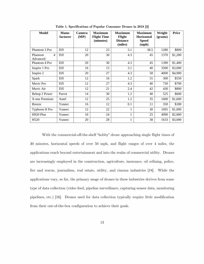
13
Table 1. Specifications of Popular Consumer Drones in 2018 [2]
Model Manu-
facturer
Camera
(MP)
Maximum
Flight Time
(minutes)
Maximum
Flight
Distance
(miles)
Maximum
Horizontal
Speed
(mph)
Weight
(grams)
Price
Phantom 3 Pro DJI 12 23 3.1 38.5 1280 $800
Phantom 4
Advanced
DJI 20 30 4.3 45 1370 $1,200
Phantom 4 Pro DJI 20 30 4.3 45 1390 $1,400
Inspire 1 Pro DJI 16 15 3.1 40 3500 $3,000
Inspire 2 DJI 20 27 4.3 58 4000 $4,900
Spark DJI 12 16 1.2 31 300 $550
Mavic Pro DJI 12 27 4.3 40 730 $700
Mavic Air DJI 12 21 2.4 42 430 $800
Bebop 2 Power Parrot 14 30 1.2 40 525 $600
X-star Premium Autel 12 25 1.2 35 1600 $1,600
Breeze Yuneec 16 12 0.1 11 350 $180
Typhoon H Pro Yuneec 12 22 1 30 1695 $1,000
H920 Plus Yuneec 16 24 1 25 4990 $2,800
H520 Yuneec 20 28 1 38 1633 $3,000
With the commercial-off-the-shelf “hobby” drone approaching single flight times of
30 minutes, horizontal speeds of over 50 mph, and flight ranges of over 4 miles, the
applications reach beyond entertainment and into the realm of commercial utility. Drones
are increasingly employed in the construction, agriculture, insurance, oil refining, police,
fire and rescue, journalism, real estate, utility, and cinema industries [18]. While the
applications vary, so far, the primary usage of drones in these industries derives from some
type of data collection (video feed, pipeline surveillance, capturing sensor data, monitoring
pipelines, etc.) [16]. Drones used for data collection typically require little modification
from their out-of-the-box configuration to achieve their goals.

14
Tech companies have initiated plans for drones that go beyond data collection,
such as Amazon’s exploration into drone-based delivery or Facebook and Google X’s
attempt to use drone to deliver Internet connectivity, but the success and sustainment of
those projects has yet to be evaluated [17].
2.3.4 Academic Interest
Multirotor copters have also been a popular topic in the academic community, with
282 IEEE publications between 2015 and 2018 using the keyword “multirotor.” Such
papers include enhancements such as infrared assisted landing [18], computationally-
efficient trajectory generation [19], video stabilization [20], automated battery swapping
[21], and multi-sensor navigation in GPS denied environments [22]. Figure 2 show numbers
of UAV papers identified from the top eight journals/conferences over the years 2001–
2016. The points have been interpolated with an exponential curve [23].
Figure 2. Number of UAV papers published from the top eight journals/conferences [23]
15
It can be expected, due to consumer and academic interest, that drone capabilities
will continue to increase in terms of autonomy, sensor accuracy, flight control, range and
flight time, resiliency, and onboard artificial intelligence.
2.4 Wireless Technologies
This section discusses technical aspects of widely used wireless technologies that
are deployed on devices ranging from routers, smartphones, drones, and other consumer
and retail devices. The most applicable to this research is Wi-Fi.
2.4.1 Wi-Fi
Wi-Fi is a popular and widely used physical and link layer specification defined by
the IEEE 802.11 (hereafter referred to as 802.11) standard [24]. The architecture is
comprised of four major physical components: (i) access points (APs), (ii) wireless medium,
(iii) stations (devices), and (iv) distribution systems (i.e., router) [25]. The wireless
medium is the electromagnetic spectrum allocated in the 2.4 and 5.8 GHz radio bands,
which are subdivided into different frequency channels. Client devices poll different
channels to find APs and attempt to make connections. APs are typically assigned a
service set identifier (SSID) to identify them locally. Devices wishing to connect to the
system must first authenticate if the system has security enabled and then associate.
2.5 Wi-Fi Security Protocols & Attacks
The next section presents security protocols implemented for Wi-Fi, known attacks against
them, and how the attacks can be augmented with the assistance of a drone.

16
2.5.1 Open Configuration
An “open” AP is one that has no encryption or authentication mechanism in place.
As a result, traffic to and from open APs are susceptible to eavesdropping and injection
attacks if not encrypted by a high-layer mechanism such as Hyper Text Transfer Protocol
Secure (HTTPS). They are also much easier for an attacker to spoof (digitally masquerade
as someone else for illegitimate gain), which can lead to Man-in-the-Middle attacks.
Despite the insecurity, open APs are common in areas that offer public Wi-Fi.
Out of user convenience, many contemporary smartphones probe for all Wi-Fi APs they
have connected to in the past using a special broadcast called a ‘Probe Request,’
unintentionally leaking the SSID of every network the phone has ever connected to. A
list of previous associations can also be used to help uniquely profile a device. Connection
authentication only requires the SSID to match, so an unassociated smartphone
automatically attempts to connect to any AP with a previously associated SSID, even if
the AP illegitimate.
For quality of service, if multiple APs of the same SSID are within range, a Wi-Fi
client chooses to associate with the stronger signal. An attacker can deauthenticate the
connection using a special 802.11 packet sent to the client. Then, the target device
attempts to reconnect to the AP of the corresponding SSID with the strongest signal. For
open APs, this presents a vulnerability because an attacker can take control of the new
session if they set up an “evil twin” (a spoofed AP with the same SSID) that is closer or
has a stronger antenna than the legitimate one [26]. An evil twin attack is one that can

17
be easily done with a drone, as drones can carry equipment capable of spoofing APs and
have mobility to attain proximity to deliver a strong signal to a given target.
2.5.2 WEP
The Wired Equivalency Privacy (WEP) was the first security algorithm for 802.11,
utilizing the Rivest Cipher 4 (RC4) stream cipher for encryption, the Cyclic Redundancy
Check 32-bit (CRC-32) checksum for integrity, and secured by a 10 or 26 hexadecimal
key. Initially designed to provide the confidentiality of a wired network, an
implementation flaw was demonstrated in 2001 that allows the key to be cracked with
cipher-text alone [27]. Because RC4 is a stream cipher, it is important to prevent an
identical message traffic key from being generated. An initial vector (IV) field is usually
supplied to prevent such repetition, however WEP uses an IV that is only 24 bits long.
According to the famous birthday paradox, of the 16.7 million possible IVs, a repeat can
be expected with a 50% probability after 5,000 frames. With 99% confidence, a repeat
happens after 12,400 frames. Since IVs are passed plaintext, it is easy for an attacker to
know when this has occurred.
Improvements to the attack, such as simulated packet replay to increase traffic
and speed up the attack and open-source hacker tools such as aircrack-ng soon showed
that WEP could be cracked within minutes. Now depreciated, WEP usage has dropped
from its peak of 45% in 2010 to 7% in 2018 [28].

18
2.5.3 WPA
While Wi-Fi Protected Access II (WPA2) was the recommended solution to WEP,
Wi-Fi Protected Access (WPA) was designed to be an intermediate solution for hardware
that could not support WPA2. Utilizing the Temporal Key Integrity Protocol (TKIP), a
new 128-bit key is generated for each packet, making WPA resilient to IV attacks that
compromised WEP.
Both WPA and WPA2 (discussed next) offer two versions tailored to different end-
user architectures: WPA-PSK and WPA-Enterprise. WPA-PSK, or WPA-Personal, is
designed for home and small office use where clients authenticate with a pre-shared key
(PSK), typically in the form of an 8-63 ASCII passphrase [24]. WPA-Enterprise is also
known as WPA-802.1X and requires an authentication server to be on the network.
2.5.4 WPA2
IEEE 802.11i-2004 is an amendment to the original standard that introduced Wi-
Fi Protected Access II (WPA2), the replacement for the broken Wired Equivalent Privacy
(WEP) and deprecated Wi-Fi Protected Access (WPA) [29]. Using the PSK or
authentication server parameters, WPA2 devices generate a Pairwise Master Key (PMK)
using a cryptographic hash function to secure communication. The PMK itself is never
sent over the wire yet can still be verified by both sides to provide secure authentication.
A temporary key called the Pairwise Transient Key (PTK) is generated from the PMK
for each connection.

19
WPA2 utilizes the Extensible Authentication Protocol (EAP) over LAN (EAPOL)
four-way handshake between the AP and client during authentication. Figure 3 depicts
the handshake, with the AP on the right and the client station on the left:
The AP first sends a one-time use, random 256-bit value called the “ANonce,” (‘A’
for AP)
The client responds with its own 256-bit random “SNonce,” (‘S’ for station) along
with a Message Integrity Code (MIC). The client can now derive the PTK from
nonce values and the two parties’ Media Access Layer (MAC) addresses.
The AP can use the ANonce, SNonce to derive the PTK as well. It verifies the
MIC. If successful, it sends over other connection parameters, to include the Group
Transfer Key (GTK).
The station verifies the MIC to ensure the AP has the correct PTK. It sends back
an ACK and a data connection can begin.
This handshake scheme is unique in that it allows both parties to independently
prove to each other they both know the correct PMK without ever actually transmitting
it. While the details are beyond the scope of this research, it is important to know that
the authentication is possible because both parties send specific messages encrypted by
the independently generated PMK. If both devices can decrypt each other’s message and
get the expected plaintext, then a secure session can begin.

20
Figure 3. WPA2 four-way handshake. On the left is the Station (STA) and the right is the
Access Point (AP)
Among other implementation changes, WPA2 utilizes the Advanced Encryption
Standard (AES) block cipher instead of the RC4 stream cipher, which increases cryptologic
diffusion.
2.5.5 WPA and WPA2 Brute Force Attacks
WPA-PSK and WPA2-PSK are considerably more difficult to compromise than
WEP, but they are still susceptible to brute-force or dictionary-building attacks [29]. Here,
an attacker must try a potential passphrase, calculate the message authenticity check in
the same way a legitimate device does, then verify if the password is correct. For WPA
and WPA2, parameters that are used in the computation must first be acquired by
capturing an initial handshake of a legitimate party. For WPA2, the EAPOL four-way
21
handshake messages depicted in Figure 3 contain all the information that is needed to
verify if a passphrase is correct. After sniffing a single legitimate handshake, the attacker
is free to passively test as many guesses as desired. This can be done without further
interacting with the network until the correct passphrase is found.
WPA and WPA2 have security measures to make this attack less effective. When
using the PSK method, a 256-bit shared encryption key is created for the AP. This is
done by concatenating the passphrase, SSID, and length of the SSID string, hashing them
4,096 times using HMAC-SHA1, then feeding the result into an RSA key derivation
function. Devices then encrypt their sessions with a 128-bit key derived from it.
The purpose of hashing 4,096 times is to slow down the speed of an attacker
attempting to brute-force guess the passphrase. An attacker must perform 4,096 hashes
for each guess, adding computational complexity required for each guess. Since the SSID
is used as a salt to the passphrase, encryption key pairs are unique to the SSID. Thus, an
attacker cannot build a universal pre-built table of passwords and their corresponding
encryptions keys (known as a rainbow table). Each table is only relevant to a specific
SSID. Still, analysis of worldwide deployments shows that the 100 most common SSIDs
compose 11.97% of all APs worldwide [28], so some pre-computed tables have generalized
usefulness. Using a valid rainbow table allows an attacker to search if a given AP uses
any of the precomputed passwords in linear time. The tradeoff with rainbow tables is the
extreme memory space required to store them as well as the time required to compute
them in the first place. Pre-computed rainbow tables for the top 1000 SSIDs and common
passwords are available online [30].

22
2.5.6 WPA3
First announced in January 2018, WPA3 offers security upgrades, such as updating
the handshake to make password brute-forcing more difficult. Since the market share that
implements WPA3 is less than 1% [28], this research does not further investigate WPA3.
2.6 IoT
Conceptually, the Internet of Things (IoT) can be summarized as the combination
of humans, dedicated physical devices, and Internet connectivity [31]. With an emphasis
on sensors, controllers, actuators connected to the Internet, IoT continues to increase the
physical influence cyberspace has on the “real world,” further empowering the cyber
domain. While this adds benefits in the form of convenience and automation for
consumers, it also increases the risk for data leakage, compromise, privacy violations, and
kinetic attacks enabled by cyber-attack [31]. Additionally, as the emerging market is fast-
paced and full of competition, cybersecurity mechanisms are typically an afterthought.
One would expect IoT locks to be reasonably secure, yet Rose demonstrated in 2016 that
12 out of 16 Bluetooth Low Energy locks could be compromised [32].
Regardless of the consequences, even conservative estimates of IoT devices projects
a number over 10 billion by 2020 [31]. With heavy integration into homes and businesses
(appliances, sensors, personal devices, cameras, smart hubs), it is vital to understand the
cyber and wireless-related risks of employing IoT devices.

23
2.7 Cybersecurity and Information Warfare
In 2001 Secretary of Defense Robert M. Gates stated, “cyberspace and its associated
technologies offer unprecedented opportunities to the US and are vital to our Nation’s
security, and by extension, to all aspects of military operations.” [33] Increasingly, the
information domain has played a larger role in US warfare. “Hacking,” a fuzzy term usually
referring to gaining unauthorized access to electronic information systems, has gone from
a fringe hobby to a formalized profession. Such expertise is leveraged offensively,
defensively, and passively. Different groups have different terms for each of these types
of activity.
Joint Publication 3-12 defines Cyberspace Operations (CO) as comprised of
Offensive Cyberspace Operations (OCO) and Defensive Cyberspace Operations (DCO)
[33]. OCO is analogous to cyber-attack (a projection of force through cyberspace), and
DCO is defensive or mitigation actions to prevent or recover from a cyber-attack. The
terms OCO and Computer Network Attack (CNA) are interchangeable. Computer
Network Exploitation (CNE) is a term used to describe digital exploitation, monitoring,
and data collection used for the purpose of intelligence gathering with no projection of
force. Sometimes intelligence gained from CNE can assist OCO, however in the context
of US operations, the two operate under different legal authorities.
As hacking has matured, so have the tactics, techniques, procedures, and
terminology [26]. Though variations exist, a common methodology is largely recognized
for the attack process that is depicted in Table 2.

24
Table 2. Hacker Methodology
Reconnaissance
Scanning / Enumeration
Gaining Access
Privilege Escalation /
Pivoting
Maintaining Access
Covering Tracks
Of the steps in the methodology, drones can provide a distinct advantage in the
first three steps: Reconnaissance, Scanning/Enumeration, and Gaining Access.
Reconnaissance is passive information gathering of a target. It is a systematic
attempt to identify, locate, and collect information. The more that is known about a
target, the easier Gaining Access is. Drones also have the advantage of mobility and
geographic awareness, allowing the ability to add geographic data (latitude, longitude,
altitude, etc.) to information collected.
The next phase, Scanning and Enumeration, is an active attempt to interact with
a computer system to elicit a response. It is used to identify relevant technical information
about a system for the purpose of gaining access. This includes identifying open ports,
applications, services, operating systems, vulnerabilities, and security measures. When
enough information is gathered, an actual attempt to gain access can be made based on
known attack vectors. This can be accomplished in many ways, to include exploitation,
social engineering, or password cracking [26].
There are many possibilities in the Scanning/Enumeration and Gaining Access
phases that an attacker could benefit from by using drone technology. A drone with a

25
properly equipped Wireless Network Interface Card (WNIC) can surreptitiously allow an
attacker to capture and interact with wireless traffic as if they are physically close (also
called Remote Physical Proximity).
Privilege escalation involves taking steps to acquire higher levels of access beyond
the level in which they first gain access, while maintaining access consists of attaining
more persistent, simpler, or redundant methods of control from the original entry vector.
Covering tracks consists of taking steps to prevent discovery by legitimate users and
administrators.
2.8 Related Research
This section investigates developments and research that employ drones for collecting or
interacting with wireless networks. Research about augmentations that could increase the
drone hacking capabilities are also presented.
2.8.1 Wireless-Sensing Drones
Some drones may be configured to have the capability to detect and monitor
wireless traffic. These can be used to target specific wireless protocols, such as Wi-Fi,
Bluetooth, or Global System for Mobile communications (GSM). The existence of drones
designed for such a purpose are rare but do exist. For instance, in 2015 a modified DJI
Phantom was used over Los Angeles by the marketing company Adnear (now renamed to
Near) to collect unique device identification data from Wi-Fi connections for the purpose
creating targeted advertisements [34].

26
Wi-Fi devices use a Wireless Network Interface Controller (WNIC) to collect
wireless traffic. WNICs are capable of up to three modes: managed, promiscuous, and
monitor mode. In normal circumstances, the WNIC is set to managed mode, which means
the card checks incoming frames for the intended destination address. A “frame” is the
name for a data-link layer message, often containing a packet of information. If the
destination field matches the device’s globally unique Media Access Control (MAC)
address, the wireless card continues to process the packet and move it up the network
stack. However, if the MAC does not match, the frame is dropped if the card is in managed
mode. If a card is set to monitor mode, it processes and stores all intelligible frames,
regardless if it is for the intended destination [22]. This allows the device to “sniff” all the
traffic in the air around it. This includes connection attempts, unique MAC addresses,
connection information, SSID broadcasts, and other significant data about local users [24].
The extent to which an entity processes and uses this data may be of interest for
privacy advocates. In the case of the Adnear drone, information was correlated to assist
in location-based advertisement targeting. The potential possibilities of what can be done
with similar data is discussed in the next section. These collections may be done with
stationary wireless devices, however a drone equipped for a similar task can cover a larger
geographic area and integrate location data. As current FAA regulations are safety-
focused and not privacy-focused, there are few checks on these drone capabilities.

27
2.8.2 Identification from Location
According to a report by Massachusetts Institute of Technology researchers,
“uniqueness of human mobility traces is high”—that is, using even course data sets and
minimal samples, it is fairly easily to identify a user by their distinct but predictable
physical location data [35]. Since smartphones and other personal devices often beacon
frames with a static MAC address, it is easy to passively collect unique location
information. Mounting that capability on a drone makes the attack even more powerful
to do with drones. The report found that any cellphone user can be uniquely identified
with 95% confidence if given just four location data points. With eleven data points, the
researchers were able to identify all 1.5 million cell users in an undisclosed “small European
country.” The dataset was not particularly extensive or complex, consisting of a list of
users tagged by their closest cellphone tower once an hour.
2.8.3 Proof of Concept: Drones That Can Hack
While much academic focus and articles exist for hacking drones (where the drone
is the target) [36], there are only a few examples of developing drones that hack (where
the drone is the attacker). However, a few examples exist.
A proof-of-concept fixed wing drone running the Backtrack 4 operating system was
developed by two security researchers in 2011. The drone weighed 13 pounds and could
allegedly intercept phone calls by mimicking a cell phone tower, among other capabilities
[37].
28
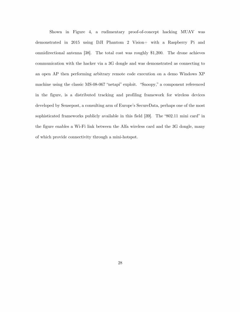
Shown in Figure 4, a rudimentary proof-of-concept hacking MUAV was
demonstrated in 2015 using DJI Phantom 2 Vision+ with a Raspberry Pi and
omnidirectional antenna [38]. The total cost was roughly $1,200. The drone achieves
communication with the hacker via a 3G dongle and was demonstrated as connecting to
an open AP then performing arbitrary remote code execution on a demo Windows XP
machine using the classic MS-08-067 “netapi” exploit. “Snoopy,” a component referenced
in the figure, is a distributed tracking and profiling framework for wireless devices
developed by Sensepost, a consulting arm of Europe’s SecureData, perhaps one of the most
sophisticated frameworks publicly available in this field [39]. The “802.11 mini card” in
the figure enables a Wi-Fi link between the Alfa wireless card and the 3G dongle, many
of which provide connectivity through a mini-hotspot.

29
Figure 4. DJI Phantom 2 Vision+ with an omnidirectional antenna payload (above) and
accompanying component schematic (below) [38]
Perhaps the most sophisticated publicly recognized hacking drone, the “Danger
Drone” is a prototype consisting of a Raspberry Pi on a custom drone created by two
researchers from Bishop Fox in 2016, presenting at the popular hacker DEFCON and

30
Black Hack conferences in 2017 [40]. Hacking capabilities are established through the
Raspberry Pi’s WNIC. The drone has a 1.2-mile range and reportedly can use a cellphone
module for control over a cellular Long-Term Evolution (LTE) connection. The total cost
of parts is listed at just below $500. The drone was presented as a penetration test tool
to measure the effectiveness of drone defense deployments.
2.8.4 Directional Antenna
A directional antenna offers a unique advantage over the more commonplace
omnidirectional antennas in that they can offer a larger sensing range. Because they also
have a limited bearing, a rotating antenna can determine the relative angle at which a
target signal is strongest. Law demonstrated a median bearing accuracy of 9° using a Yagi
directional antenna connected to a stepper motor and Raspberry Pi [41]. With multiple
data points at multiple different locations, bearing and signal strength could be used to
triangulate the actual position of a target.
2.8.5 Data Leakage
After capturing Wi-Fi and Bluetooth Low Energy (BLE) frames of a smart home
in 2018, Beyer created a program that can correctly classify devices with a 94% accuracy
for Wi-Fi and a 75% success rate for BLE [42]. On average, the research demonstrated a
95% accuracy at detecting events such as a door opening or camera detecting motion.
This was done even when the connections were encrypted—the data was derived purely
from low-layer headers and other traffic properties such as frame size and rate. The

31
researcher further correlated the events to accurately assess pattern-of-life information
about the human user’s daily schedule.
A similar mechanism can easily be employed on a drone to track pattern-of-life
information of users and devices in a much larger geographic radius. If combined with a
directional antenna, this could be done covertly by being multiple times away from the
standard maximum range of 100 meters.
2.9 Background Summary
This chapter provides a brief summary of current military drone and commercial
drone usage and capabilities. Wireless technology with an emphasis on Wi-Fi is discussed,
along with associated security protocols and known attacks. The growing cyber-physical
crossover caused by the rise Internet of Things (IoT) is explored. A primer on Cyberspace
Operations and the role drones offer to enhance cyber-attack capabilities are explored,
followed by developments and research areas that demonstrate drones currently
participating in a similar capacity. This research contributes to the areas of drones,
wireless technology, and cybersecurity.

32
3. III. Prototype Design
3.1 Overview
This research presents and analyzes data obtained from two different hardware and
software prototypes:
localizer – a stationary, rotating directional Wi-Fi collection device. The antenna
is rotated by a stepper motor and controlled by code written in Python. This is the same
device and software used in Law’s thesis on “Passive Radiolocation of IEEE 802.11
Emitters Using Directional Antennae” [41].
This research builds on Law’s previous work by investigating the collection device’s
viability at geolocation and bearing prediction accuracy at further distances. While
equipped with a GPS module, localizer framework cannot determine compass bearing
on its own and needs to be calibrated each time it is moved.
skypie – a lightweight, directional Wi-Fi collection device developed during this
research. This prototype is the next iteration of localizer, with a focus on being viable
for drone operations. Pilot tests indicated that using a stepper motor like that in
localizer is excessively heavy and would make onboard compass readings
unpredictable, so the antenna is fixed. Mobility and rotation will be accomplished through
the rotation of the drone.
The skypie sensor payload is equipped with its own GPS and accelerometer, offering
complete independence from the drone’s control architecture. The sensor can operate
either autonomously or be controlled via configuration and commands sent over a 3G/4G

33
link. The codebase, written in Python, also contains skyport, a Python-based set of
web applications that can process and analyze data from multiple sensors and provides a
Graphical User Interface (GUI) for interacting and controlling skypie sensors.
The localizer prototype is shown in Figure 5 and described in Section 3.2.1,
and the skypie prototype is shown in Figure 6. Figure 7 depicts an ‘exploded’ version
of the skypie hardware components for ease of viewing, which are described in Section
3.4.
Figure 5. localizer prototype
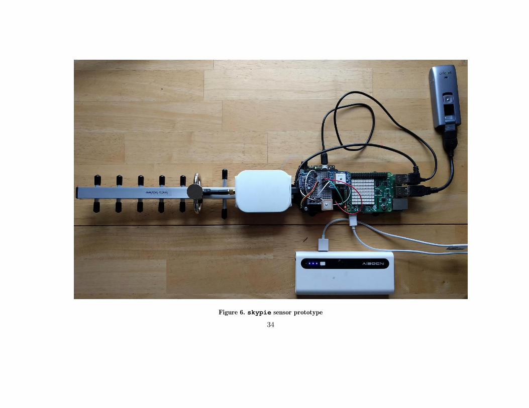
34
Figure 6. skypie sensor prototype

35
Figure 7. Hardware components presented in an ‘exploded’ fashion for ease of viewing

36
3.2 System Summary
3.2.1 localizer Summary
As shown in Figure 5, the localizer prototype consists for a Yagi antenna and signal
receiver mounted to a rod spun by a high-precision stepper motor. The stepper motor is
powered by a 13 V DC power supply. Movement is managed by a stepper motor driver
which is controlled by a Raspberry Pi via the General Input and Output (GPIO) pins,
connected via the ribbon cable and breadboard. The Raspberry Pi is running the Raspbian
Operating System (OS) powered by a separate Universal Serial Bus (USB) battery. Using
an Ethernet cable, a user can connect to the Pi over Secure Shell (SSH) and initiate the
localizer Python program, which performs packet and GPS captures. The Wi-Fi signal
receiver and GPS module are used to digitize and analyze Wi-Fi packets and GPS signals.
Figure 8 displays the prototype schematic of localizer.
For the standard use case, localizer takes in capture parameters such as sweep
duration and angle. It uses multithreading to simultaneously start a packet capture,
capture data from the GPS module, and spin the antenna. Upon completion, it processes
each SSID beacon packet it sees, mapping the RSSI values over the time of the capture.
It then returns the compass bearing at which it interpolated the highest RSSI value for
each SSID using a Piecewise Cubic Hermite Interpolating Polynomial (PCHIP)
interpolation algorithm. Because of size and weight additions necessary for the stepper
motor (to include the stepper motor driver and 13V power source), the device is prohibited
from practical used on a commercial MUAV.

37
Figure 8. localizer prototype schematic [41]

38
3.2.2 skypie System Summary
Figure 9 displays a high-level summary of the skypie/skyport system design,
which is described in this section. Components outlined in solid blue are a part of the “kill
chain” but not inside the system design. Components outlined in a dashed blue line are
part of the system design but are not within the scope of this research.
The system is divided into two major components: the remote sensor (skypie
payload) mounted to an MUAV, and the attacker’s workstation, which runs skyport to
analyze sensor data and control remote sensor behavior. Each skypie payload has sensors
for collection, data files, and a communication mechanism for uploading and downloading
data. Data is exfiltrated over a cellular or Wi-Fi link to the Internet, with an Internet-
facing server acting as intermediary. The attacker downloads raw data files to their
workstation with the skyport software, which runs analysis and correlation algorithms.
Results are displayed in a web application (web app). Results such as geolocation history
and geolocation prediction are available to view over satellite imagery.
A typical use case is for a cyber attacker to deploy the sensor payload, amiably
named a skypie, by mounting it underneath a medium to large MUAV. As the drone
operator (who may or may not be the cyber attacker) flies the drone, the sensor captures
Wi-Fi traffic as PCAP files in monitor mode. It also records GPS data (location, speed,
angle, etc.) and magnetic compass bearing. New data files are then uploaded via either a
cellular network connection from a USB modem, a separate Wi-Fi connection, or are stored
39
locally until a connection becomes available. Files are uploaded securely to an Internet-
facing Secure File Transfer Protocol (SFTP) server. Each distinct sensor logs into a
directory assigned to it with a unique password.
The cyber attacker can then use the skyport software. With the ‘master’ SFTP
credentials, skyport downloads data from each sensor and execute analysis algorithms
on new data, such as geolocation prediction. The cyber attacker can view the drone’s
location history, configuration parameters, and analysis findings via a user-friendly web
app hosted locally on their machine. The web app overlays telemetry information over
satellite imagery to assist in CNA/CNE operations.
Note the attacker’s workstation never directly contacts the remote sensors, and
additional steps can be taken to obscure attribution so the attacker can remain
anonymous.
The cyber attacker can remotely change many of the sensor’s collection parameters,
such as adding a Wireshark filter to Wi-Fi collection (to target specific traffic or save
space), modify storage buffer sizes, toggle collection modes, alter upload and download
intervals, and put the sensor into a ‘sleep’ mode, to name a few options. The cyber
attacker can also send shell commands and scripts to be executed on the sensor even if the
sensor is currently offline. These activities can be accomplished in the web app’s graphical
User Interface (UI), or via modifying text-based configuration files that are uploaded to
the SFTP server. The next time the sensor checks in, it sees new requests and executes
them. Remote logs and command output are downloaded and available for viewing in the
same fashion.

40
Extended uses for the skypie/skyport framework are explored in Chapter 6.
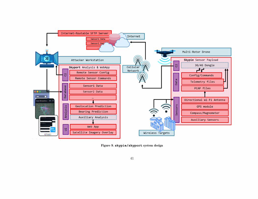
41
Figure 9. skypie/skyport system design

42
3.3 Design Goals
3.3.1 localizer Design Goals
According to Law [41], design goals for the localizer prototype are as follows:
i. Low Cost. A significant consideration for this research is the potential for low-cost
applications. Prototype hardware is limited to commercial commodity hardware,
and selection of the software framework and any libraries imported into the
software project is limited to free open source software.
ii. Low Weight. This research intends to explore ways to quickly and accurately
locate distant Wi-Fi access points from a UAV platform. Prototype hardware is
selected that mimics the capabilities of a drone platform, namely low weight and
antenna rotation control. Maximum prototype payload capacity is limited to 500 g,
a reasonable payload for medium to large consumer UAVs [43].
3.3.2 skypie Design Goals
The prototype introduced by this paper is built upon the following design goals:
A Low Cost. Similar to localizer, skypie is developed with a target cost lower
than $500 to represent the capabilities that can be attained from motivated but
poorly resourced attacker. Note these costs do not include the drone itself.
B Realistic Utility and Robustness. This goal stresses the applicability for realistic
CNA/CNE drone-based operations. It has several implications:

43
i. Sensor should operate autonomously or be able to be controlled remotely
over a secure wireless channel. If communications are interrupted, they
resume when available.
ii. Sensor should be capable of near-real time data feedback and control.
iii. Sensor should be able to operate and collect for multiple hours. This
includes sufficient battery life during collection and local storage capacity.
C Drone Architecture Portability. Appliance should not be dependent on any other
feature of the drone other than its capability to strap it on and carry it. This
means the payload must have its own GPS module, accelerometer, and means for
wireless command and control (C2) reachback to the attacker. This design goal
causes important hardware and software changes to the design from the
localizer prototype. The advantage of drone architecture independence is
interoperability with any drone capable of carrying the weight. This is preferable
because a payload using onboard drone features is likely be confined to one type
of drone or control protocol, causing the device to have a higher chance of becoming
outdated.
D Low Weight. Where the localizer design assumes telemetry and
communication functions are to be performed by the attached drone, in accordance
with Design Goal C, skypie requires additional components to give it
independence from the drone. A 2017 review of commercial drones payload
capabilities reveals that payloads up to 1 kg are supported by many medium to

44
large consumer drones, with higher end drones capable of up to 9 kg [44].
Maximum prototype weight is limited to 1 kg in this research.
3.4 skypie Hardware Design
Hardware components are chosen carefully to meet the design goals. Table 3 depicts
a chart of all major hardware components, the specific models used, weight, and price at
time of writing. Figure 10 shows a detailed schematic of how the hardware components
are connected to each other.
Figure 10. skypie payload hardware schematic
Wi-Fi Antenna. While there are many directional antennas, the Danets USB-
Yagi TurboTenna antenna is chosen because of its small size (31.5 cm in length),
low weight (137 g), inexpensive price, and commercial availability. The cross
section is small, which is beneficial for MUAV flight in windy environments. The

45
Table 3. Prototype Hardware Overview
Item Model / Version Weight (g) Price
Wi-Fi Antenna Danets USB-Yagi TurboTenna 137 $113
Wi-Fi Signal
Receiver USB WiFi Interface - DNX10NH-HP* 35 N/A
Computer Raspberry Pi 3 Model B+ V1.2 68 $35
Digital Storage 16 GB SanDisk Ultra microDSCH UHS-1 1.7 $8
Microcontroller Adafruit Metro 328** 16.5 $18
GPS External
Antenna
Passive GPS Antenna uFL - 15mm x 15mm
1 dBi gain 5.5 $4
GPS
Adafruit Ultimate GPS Breakout - 66
channel w/10 Hz updates - V3 8.5 $40
Accelerometer
Adafruit Triple-axis
Accelerometer+Magnetometer (Compass)
Board - LSM303 2 $15
Power Supply
Aibocn Power Bank 10,000 mAh External
Battery Charger 247 $12
Reachback
Communication
Unlocked Modem USB 4G LTE Huawei
E397u-53 (T-Mobile, US only)*** 51 $25
Optional Sensors Raspberry Pi Sense HAT 20.4 $38
Structure 3D printed casing 52 $2
Structure Mini-breadboard 13 $2
Miscellaneous
Components
Screws, bolts, wiring, headers, USB cables,
soldering 36 $16
Total (without Power Supply) 447 $316
Total (with Power Supply) 693 $328
*Price included with antenna
**Metro 328 can be replaced with Adafruit Metro Mini (3 g, $12). The full size is chosen for
developmental accessibility only.
***Usage of the 3G/4G modem is not in the scope of this research

46
high-power beam width is approximately 56° with a gain of 18 dBi [45]. The
antenna functions in the 2.4 GHz band.
Wi-Fi Signal Receiver. The DNX10NH-HP USB Wi-Fi network interface comes
packaged with the Yagi TurboTenna and reliably works out of the box with the
Raspbian OS. It compares well to the popular Alfa AWUS036H USB wireless
adapter commonly used for wireless cyberspace operations [41].
Computer. The Raspberry Pi 3 Model B+ is an opportune platform for this
application because of its low price point ($35), low weight (45 g), sophisticated
features, and supported ecosystem. The abundance of USB ports and GPIO pins
make it flexible for adding additional sensors.
Microcontroller. While the Raspberry Pi functions as a full operating system, it
does not offer real-time support for hardware modules. Many sensors, stepper
motors, and other electronic components require a real-time controller to
function. To accommodate the need for the GPS module and accelerometer, plus
any hardware added later, the Adafruit Metro 328 is chosen because of its
compatibility with the ubiquitous Arduino Uno (sharing the same Atmega328
chipset) and for the ecosystem it shares with other Adafruit components. The
Metro 328 can be programmed using the free Arduino Integrated Development
Environment (IDE). Power and programming can be accomplished via the
onboard micro USB port, which also doubles as the power source. The Metro
328 is also available in a smaller form factor (3 g, $12), however for accessibility
of development, the larger size is chosen (16 g, $20).

47
Global Positioning Module. This Adafruit Ultimate GPS Breakout (66 channel
with 10 Hz Updates Version 3) device is chosen over the cheaper GlobalSat BU-
353S4 ($31) used in localizer. This choice is made to reclaim one of the USB
ports being used on the Raspberry Pi, as well as to couple the accelerometer and
GPS data into a single data feed, which is sent from the controller to the Pi. The
Ultimate GPS Breakout is also technically superior to the GlobalSat BU-353S4,
notably offering 10 updates per second if desired. A passive GPS Antenna uFL
1 dBi gain antenna is attached to boost reception.
Accelerometer. The Adafruit Triple-axis Accelerometer+Magnetometer
(Compass) Board is chosen because of its tiny form factor, ease of interaction,
pre-built libraries, and satisfactory factory calibration settings. The underlying
chip is the LSM303.
Power Supply. The ideal power supply minimizes weight while maximizing power
capacity. At 272 g and 10,000 mAh for $12, the Aibocn Power Bank External
Battery Charger is acceptable.
Reachback Communications. Though not in the scope of this research, the
skypie payload is designed to be able to receive and transmit data via a 3G or
4G link. This can be done using a modem-mode 3G or 4G USB dongle and a
Subscriber Identify Module (SIM) card with the appropriate data plan and service
provider [46]. For experiments in this research, this link is simulated by the Wi-
Fi connection using the Raspberry Pi’s native Wi-Fi interface (not the Yagi

48
antenna used for collection). According to Design Goal B i, the unit should still
operate if cellular coverage is not in the area or if the link does not exist.
Optional Sensors. This prototype includes a Raspberry Pi Sense Hardware
Attached on Top (HAT), which was originally used for the compass sensor
(ultimately not chosen because of the extensive calibration needs and software
decencies), but kept for the 8x8 Red-Green-Blue (RGB) Light-Emitting Diode
(LED) array. The LED array is useful for indicating the state of the device in
development mode. The board also offers pressure, humidity, and gyroscopic
sensors which are not currently used.
Structure. A 3D-printed plate is designed to securely hold the components. It
is printed using Polylactic Acid (PLA) biodegradable filament. The design is
shown in Figure 11. Figure 12 shows where each piece fits on the assembled
prototype.

49
Figure 11. 3D printed structure components
Figure 12. Structure components assembled on prototype

50
3.5 skypie Software
Prototype skypie software is written almost entirely in Python. The
microcontroller code and geodesic intersection algorithm are written in C++. The
codebase is a single repository divided into three packages: skypie, skyport, and
shared. Important components and features of each packages are described in the next
sections. The source code is not included in this document due it exceeding 4,200 lines of
code.
3.5.1 Design Paradigm
To meet the design goals in Section 3.3.2, the software is designed with the following rules:
Controllable settings of the sensor are in the form of a configuration file. This is
how the attacker can control the behavior of sensor-related functions. An example
of a skypie configuration is available in Appendix A.
The program control is modeled as a control loop. At the beginning of each loop,
the latest version of the configuration file is loaded.
Subtasks (such as Wi-Fi collection, telemetry collection, file upload or download)
are initiated using parameters (such as Wireshark filters, duration, interval) as
specified by the latest configuration file.
o These changes are only actuated when the previous iteration of the same
task has been completed. This is chosen to benefit system stability and is
a preferred Python programming practice.

51
Tasks are completed asynchronously as threads. This takes advantage of multi-
threading and allows multiple operations to occur at once.
For collection-based tasks (such as Wi-Fi and telemetry), data files are written to
a separate file per thread. This means data file sizes are managed by changing
collection intervals. Files are named by start time.
Tasks are broken into finite, interval-based tasks. This is chosen to prevent
interrupting threads. The disadvantage is that data may be missed in between the
short transition periods. The advantages include increased code readability,
simpler implementation, better programming practices, and less potential for data
corruption.
Because both the sensor and the attacker are likely to not have static Internet-
facing IP addresses, a public server is required to act as a ‘dead drop’. In practice,
this is a web server the attacker has set up. The sensor uploads data using SFTP,
and the attacker can login and download data from the sensors at any time.
Analysis is performed on the attacker’s workstation. The attacker uses a secondary
program (skyport), which utilizes the same looping and threading mechanism in
the sensor. In this case, the control loop is responsible for managing uploads,
downloads, and analysis on new files according to its skyport configuration file.
An example of a skyport configuration file is available in Appendix A.
If the sensor software is somehow killed, a chron job reinitiates it after 60 seconds
and resumes operation. If the attacker wants to keep the sensor dormant, they
can choose to put it in ‘off’ mode. Therefore, the sensor turns on every 60 seconds,

52
checks for an update, and turns back off. This is to support persistence and extend
battery life. The chron job also initiates skypie software at bootup.
The user interface should be friendly and as portable as possible to show 1) viability
as a useful operational attack tool and 2) how easily cyber-attack drones can be
harnessed by any threat actor once developed.
3.5.2 skypie Package
The skypie package contains code that runs exclusively on deployed sensor device
(the Raspberry Pi) and has specific software requirements. Those requirements are listed
in Table 4. Important design components of the skypie package are described in the
following sections.
Table 4. skypie dependencies
Package Function
iwconfig Get Wi-Fi adapter settings, set monitor mode/channel
iwlist Get Wi-Fi interface current channel
ifconfig Prepare Wi-Fi interface for monitor mode
dumpcap Capture packets from Wi-Fi interface
tshark Makes packet captures available to Python for analysis
3.5.2.1 main.py
This module parses parameters and starts the execution of the manager module.
Several parameters the program supports are “-a” which activates the main control loop,
“-n”, which does not wait for a GPS satellite fix before starting, “-d” which shows
debugging messages, and “-x”, which starts self-destruct mode. Self-destruct mode will

53
replace the sensor’s hard drive with 0’s until the system crashes. Self-sabotaging
commands can also be executed remotely utilizing the command.py module described in
Section 3.5.2.5.
3.5.2.2 manager.py
This module controls the activities of the rest of the program. Essentially, the
other modules in the package offer services, such as Wi-Fi collection, telemetry collection,
or data transfers. The manager module is responsible for keeping those services running
as directed by the sensor configuration file. This behavior is summarized in Figure 13 and
is further explained in the rest of Section 3.5.2.
Figure 13: skypie control flow diagram

54
Upon initiation by main, manager sets up data folders and checks for the skypie
sensor configuration file (./synch/config.txt), which has customizable parameters
for operation. An example configuration file is given in Appendix A. Altering the
configuration file is the recommended way to change sensor behavior. manager reads the
current configuration (loading a default version if none exists), then creates a dictionary
of threads for each important function. Each iteration of the loop checks for changes to
the configuration file and starts new threads as needed.
Threaded tasks are intended to be finite and expire (for example, “collect Wi-Fi
packets for 60 seconds”). When a thread completes, the main loop sees the expired thread
and start another thread (for example, “collect for another 60 seconds”). If the attacker
decides to turn off Wi-Fi collection, manager sees the Wi-Fi collection config value is now
‘off’, and does not initiate a new collection thread until that value is ‘on’ again. This is
the same behavior that dictates all configuration changes. Note that once a thread is
started, it is not interrupted, new settings apply only after the current thread has
completed. This choice is made for system stability.
3.5.2.3 collection.py
This module handles collection of Wi-Fi packets by making a subprocess call to
dumpcap after setting the selected interface into monitor mode. Parameters, such as
Wireshark filter and duration are passed along. File output locations, including the entire
data storage scheme are shown in Appendix A.

55
3.5.2.4 telemetry.py
This module handles parsing telemetry data, which comes from the microcontroller
over a serial connection from the fourth USB port (/dev/ttyUSB0). Sentences are
customized to this application, stripping National Marine Electronics Association (NMEA)
data for relevant fields and adding the compass bearing from the accelerometer. An
example of a skypie telemetry sentence is show in Figure 14, displaying fields, the index
at which they can be found, and example values. Fields in indexes 4-6 are added for
consistency with localizer GPS data even though the skypie sensor does not populate
them.
Figure 14. ‘SKY’ telemetry sentence
Under normal operation, manager requests the GPS module to acquire a satellite
fix and return a current timestamp before the main loop starts. The OS then uses that
timestamp to update the system clock. This ensures packet captures and telemetry data
are synchronized as much as possible, which is critical for accurate packet-telemetry
analysis.
3.5.2.5 command.py
This module contains a thread class that checks for new script files sent from the
attacker. The commands are executed in a subprocess at the same privilege level as the

56
skypie code (root). The output is written to a text file, which is placed in the
‘./data/synch/log’ folder for upload back to the attacker’s workstation.
3.5.2.6 interface.py
This module parses ifconfig and iwconfig data and offers support for
changing available wireless interface settings. The antenna interface used for collection is
selected by manager using this module (specified by the config.txt file), and whenever
a capture is performed this module puts the interface in monitor mode. This module also
contains a thread class that asynchronously cycles through 802.11 channels, which is
invoked consistently through the manager module’s main control loop. When the
application closes, the interface is restored to managed mode.
3.5.2.7 indicator.py
This module contains code that checks for the presence of the Raspberry Pi Sense
HAT, which is an optional hardware component. If present, the 8x8 RGB LED array
illuminates to signify what actions are happening in the main loop. This visual is useful
in a development and testing environment, but may not be desired in real operations.
Table 5 demonstrates what the different patterns mean. Behavior of a normal capture
operation appears as fast-moving purple numbers and occasional flashes for green, blue,
and pink.
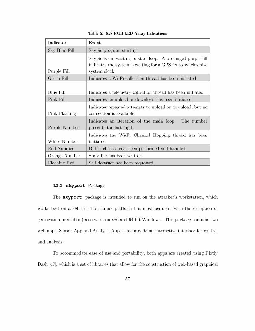
57
Table 5. 8x8 RGB LED Array Indications
Indicator Event
Sky Blue Fill Skypie program startup
Purple Fill
Skypie is on, waiting to start loop. A prolonged purple fill
indicates the system is waiting for a GPS fix to synchronize
system clock
Green Fill Indicates a Wi-Fi collection thread has been initiated
Blue Fill Indicates a telemetry collection thread has been initiated
Pink Fill Indicates an upload or download has been initiated
Pink Flashing
Indicates repeated attempts to upload or download, but no
connection is available
Purple Number
Indicates an iteration of the main loop. The number
presents the last digit.
White Number
Indicates the Wi-Fi Channel Hopping thread has been
initiated
Red Number Buffer checks have been performed and handled
Orange Number State file has been written
Flashing Red Self-destruct has been requested
3.5.3 skyport Package
The skyport package is intended to run on the attacker’s workstation, which
works best on a x86 or 64-bit Linux platform but most features (with the exception of
geolocation prediction) also work on x86 and 64-bit Windows. This package contains two
web apps, Sensor App and Analysis App, that provide an interactive interface for control
and analysis.
To accommodate ease of use and portability, both apps are created using Plotly
Dash [47], which is a set of libraries that allow for the construction of web-based graphical

58
applications entirely in Python. It is also tied to the plotly library, suitable for
generating charts, graphs, and maps. Mapbox [48] is used for adding satellite overlays
because it offers a free and customizable map API compatible with plotly graphs.
The two apps operate separately or simultaneously. The skyport manager is
only required to be running if real-time updates are desired, so each of the three modules
can be ran as independent programs or in unison.
3.5.3.1 Background Control (manager.py)
In a similar fashion to the skypie/manager.py, this module acts as the driving
control module. It uses a thread dictionary to ensure data upload, download and analysis
operations are executing as directed by a configuration file. Data files are stored as Comma
Separated Value (CSV) files or PCAP files. State data, logs, and config files are stored as
text files. The program organizes data by sensor name and data type. The file structure
is show in Appendix A.
3.5.3.2 Sensor Control and Tracking App (sensor_app.py)
The purpose of this app is to view sensor geolocation history, change configuration
settings, view the sensor log, and send remote arbitrary commands via a web console. It
can be run with python sensor_app.py, which starts a webserver at
127.0.0.1:7771. Figure 15 depicts the UI, which is designed to make the user feel
“creepy, but friendly.”

59
Figure 15. Sensor App User Interface

60
The Sensor App consists of two major components, the Control Settings (on the
left), which allows a user to control Skypie behavior settings, and Sensor Tabs (on the
right), which allows the user to view location history, execute remote commands, view
remote logs, and calibrate the device. A dropdown at the top allows the user to select
which sensor they are interacting with, if there are multiple.
When the UI detects changes to any input fields, it actuates change. For example,
if the user selects a new sensor in the sensor selection dropdown, the program reads data
files for the chosen sensor, in this case, a geographic history CSV file for a sensor named
‘crunchy’), and plots the coordinates on a map in the Telemetry tab. Figure 16
demonstrates how the UI elements relate to the simple flat file ‘database’ scheme of sensor
data.
Figure 16. In-app sensor selection dropdown (left) and the skyport/database/sensors/
directory (right), showing that database is saved as a simple folder scheme.
Figure 17 demonstrates a test run of the sensor and the plot of telemetry data in
the Telemetry tab. Location history is shown as a series of dots indicating color coded by
timestamp. The latest location and heading are printed at the top of the tab.

61
Figure 17. Geolocation history can be viewed in the ‘Telemetry Tab.’ Hovering over each coordinate shows a box that describes the exact time
and location of that point. Dots are color coded chronologically. The last recorded coordinates and bearing are printed at the top of the tab.

62
There is also an option to view the heading of the sensor at different points in time
using the ‘Line Draw Density’ slider. Heading is represented as a purple line originating
at the sensor’s location extending in the direction it was facing at that point in time. This
is depicted in Figure 18.
The remote sensor’s skypie program log can be viewed via the ‘Log’ tab, as shown
in Figure 19.
Arbitrary remote commands can also be uploaded and executed on the remote
sensor using the ‘Console’ tab. An example of this is demonstrated in Figure 20.
The Control Settings tabs are shown in Figure 21 and Figure 22. Figure 21 displays
the Sensor Control tab, which is used to change properties such a file transfer settings,
webserver settings, and the device’s name. Figure 22 shows the Wi-Fi Control tab, which
can be used to change the Wi-Fi collection mode and filters.
The user can modify and setup sensor operation settings by using the UI fields in
the Control Settings tabs and clicking the ‘Submit’ button. This action modifies the sensor
configuration file on the attacker’s workstation, which is then uploaded to the SFTP server
by manager and is downloaded to the sensor when it checks in.

63
Figure 18. View history of compass heading ‘Heading Line Draw Density’ value slider. Each purple ray extends from a coordinate in time and
indicates which way the sensor was facing. In this example, the antenna is mounted to a bicycle doing a half-circle.

64
Figure 19. ‘Log’ tab enables user to view remote sensor’s skypie logs.
Figure 20. Using the ‘Console’ tab to execute ‘ifconfig’ and ‘whoami’ commands.

65
Figure 21. ‘Sensor’ settings tab, which allows the attacker to make configuration changes.
Changes are posted by clicking the ‘Submit’ button.

66
Figure 22. ‘Wi-Fi’ settings tab. Note Mirror mode and Bluetooth mode are stubs that
are not implemented in the scope of this research (discussed in Chapter 6).
3.5.3.3 Analysis App (analysis_app.py)
The Analysis App is used to view the data collected by skypie sensors. Figure
23 shows the Analysis App UI. The Analysis App consists of a Target Map pane (left)
and a Target Analysis pane (right). At the top is a dropdown selector, allowing the user
to choose which sensors to query. Data is fused from each selected sensor’s data. One or

67
multiple targets can be selected by unique MAC using the “Available Targets” dropdown,
shown in Figure 24. In this way, a user can view information collected about one targeted
device from multiple sensors. A time slider also allows an analyst to focus on a specific
timeframe, which is useful if the target is a mobile device such as a phone. The UI also
denotes which timeframes the sensors have data collected for the target. The time slider
is show in Figure 25.
Information about the first target in the “Available Targets” dropdown is displayed
in the Target Analysis pane. There is the potential for many other features to be added
to Target Analysis pane, such as correlating clients that have been seen communicating
together or what a specific target device has connected previously as indicated by 802.11
Probe Requests. These possibilities are discussed in Section 6.5. Currently, geolocation
prediction is the only feature built-in, which is processed via the analysis.py module
using the algorithms described in Section 3.6. The skyport Analysis App operates
similar to the Sensor App and can be accessed at 127.0.0.1:7773.

68
Figure 23. skyport Analysis App UI

69
Figure 24. Available targets from each selected sensor are populated in a dropdown in the
Analysis App. One, multiple, or all can be selected.
Figure 25. The timeline section indicates when a target was first and last seen. Using the slider
allows a user to pick which timeframe they want to analyze the target.
3.5.4 shared Package
The shared package contains utilities that can be shared between the deployed
sensor and the attacker’s workstation.
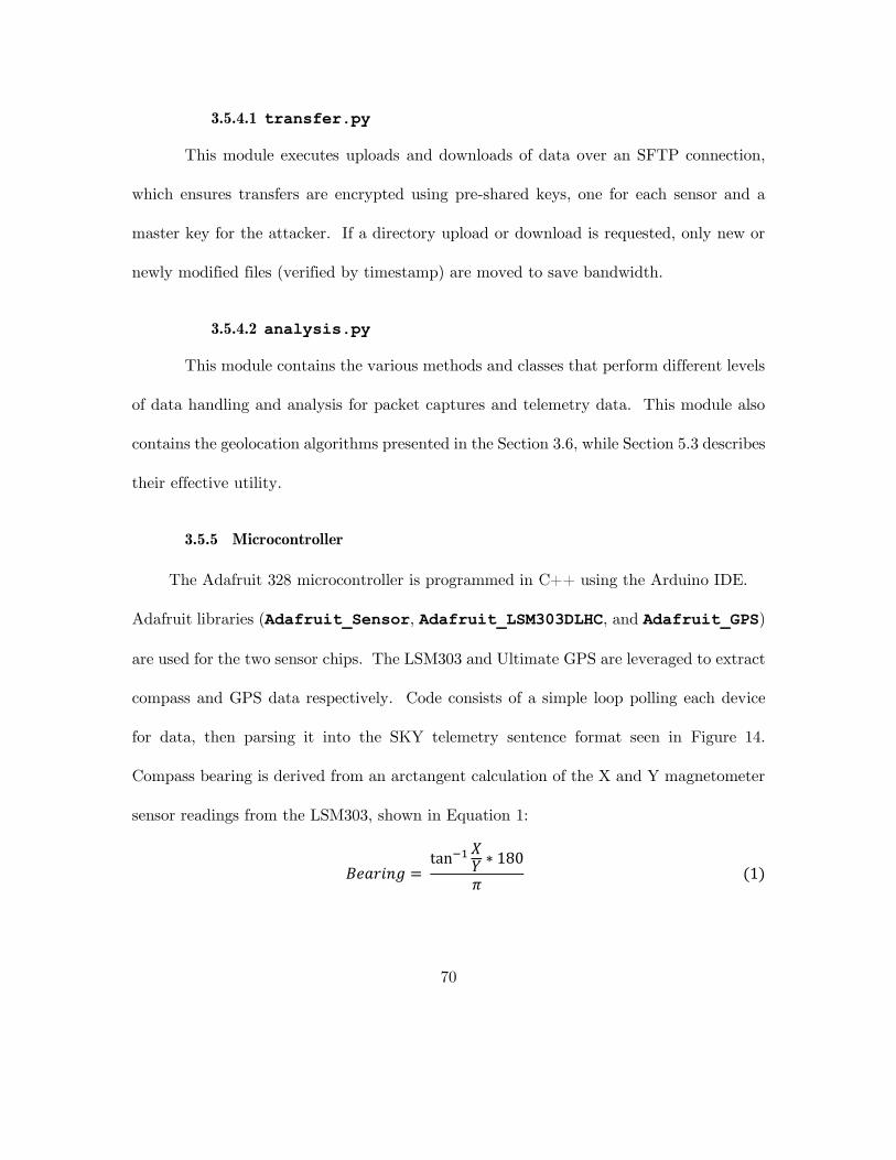
70
3.5.4.1 transfer.py
This module executes uploads and downloads of data over an SFTP connection,
which ensures transfers are encrypted using pre-shared keys, one for each sensor and a
master key for the attacker. If a directory upload or download is requested, only new or
newly modified files (verified by timestamp) are moved to save bandwidth.
3.5.4.2 analysis.py
This module contains the various methods and classes that perform different levels
of data handling and analysis for packet captures and telemetry data. This module also
contains the geolocation algorithms presented in the Section 3.6, while Section 5.3 describes
their effective utility.
3.5.5 Microcontroller
The Adafruit 328 microcontroller is programmed in C++ using the Arduino IDE.
Adafruit libraries (Adafruit_Sensor, Adafruit_LSM303DLHC, and Adafruit_GPS)
are used for the two sensor chips. The LSM303 and Ultimate GPS are leveraged to extract
compass and GPS data respectively. Code consists of a simple loop polling each device
for data, then parsing it into the SKY telemetry sentence format seen in Figure 14.
Compass bearing is derived from an arctangent calculation of the X and Y magnetometer
sensor readings from the LSM303, shown in Equation 1:
𝐵𝑒𝑎𝑟𝑖𝑛𝑔 = tan−1 𝑋
𝑌 ∗ 180
𝜋 (1)

71
Communication from the GPS chip to the microcontroller occurs at 9600 baud, and
updates are polled once a second. The chip is capable of more frequent polls if desired.
Communication to the Raspberry Pi is a serial connection over USB at 115200 baud.
3.6 Analysis Algorithms
The following sections the rudimentary algorithms that are created as a starting point
for radiolocation with a directional antenna on a moving platform. They are implemented
in the shared package.
If a sensor is stationary and has been calibrated, the ability to determine bearing
of a target is straightforward if it experiences a full 360° sweep. The sensor plots RSSI
over the bearing, and returns the value where the interpolated RSSI peaked. The process
is shown in Figure 26, where the actual beacon data points are green dots and connected
by two interpolation algorithms (PCHIP and Bernstien polynomial). The true bearing is
represented a solid vertical line while the bearing predictions are shown by dotted vertical
lines.

72
Figure 26. RSSI mapped over bearing during a 360° sweep [41].
When independently mounted to a drone, the task is complicated by the fact there
is no guarantee the antenna gets to experience a 360° sweep at every location, nor that it
gets a 360° sweep at all. Instead, the payload is given a flightpath that changes location
sometimes, changes bearing other times, changes both, and sometimes is completely
stationary.
3.6.1 Bearing Prediction and Geolocation Algorithm 1 (BPGA1)
BPGA1 takes a basic approach to return a result despite the challenges discussed.
A pictorial overview of the algorithm is shown in Figure 27, breaking it down into steps.
First, BPGA1 takes all packets it has seen over a predefined ‘bucket’ of time (60
seconds), and only considers the top 20% of those with the highest RSSI for each target.
This is because if the drone is rotating, it is assumed the true bearing of the target is the
direction from which the antenna receives the strongest signal. Second, each packet is

73
correlated to a SKY telemetry sentence by timestamp. Third, a geodesic intersection is
calculated for each of the top packet locations and supposed bearings (capped at 100
calculations per unique MAC address) giving a coordinate prediction for each pair of
packets. Predictions farther than a certain threshold (3 km) are thrown out to prevent
blatantly incorrect guesses from ruining the average.
Fourth, a weight (𝑤𝑖) is generated for each prediction and is directly proportional
to the magnitude of the distance between the two points (𝐿𝑎𝑡𝑖 and 𝐿𝑜𝑛𝑖).
Fifth, the prediction from each pair is combined into a weighted average
(𝐿𝑎𝑡𝑎𝑣𝑔 and 𝐿𝑜𝑛𝑎𝑣𝑔) using the formula in Step 5 of Figure 27 and the weights from Step
4. The rationale is that predictions taken from measurements farther apart from each
other may be more accurate given imperfect bearing predictions. The summation is
normalized by the sum of the weights (𝑤𝑇) to return a coordinate prediction.
Finally, the algorithm also returns the largest difference in radio values (Radio
Confidence) during the time bucket as well as the largest distance between two coordinates
used (Geolocation Confidence). These values are used as rudimentary confidence metrics,
under the assumption that more geographically separated observations are more valuable.
Higher radio differences are desired because they imply sensor rotation, thus increasing
the likelihood the bearings used to calculate the predictions are correct.
These values are calculated for each device for each time bucket and are stored in
./sensors/[sensor_name]/analysis/geo-mac-analysis.csv for the
Geolocation Prediction Averaging Algorithm 1 (GPAA1) to use.

74
This algorithm is implemented in the calculateLocation() function of the
MacInfo class of analysis.py.
3.6.2 Geolocation Prediction Averaging Algorithm 1 (GPAA1)
GPAA1 is invoked when a user is viewing targets in the Analysis App. It takes the
output of BGPAA1 from each selected sensor, which consists of a coordinate prediction
for each time bucket and associated weights for both distance and radio difference seen
from that bucket.
Using those values, GPAA1 looks only at the timeslice selected by the user and tries
to form a single geolocation prediction. It does this by weight averaging each BPGA1
geolocation prediction. Guesses taken from larger distances and larger radio power
disparities are given the most weight. Weights are first divided by a maximum value (3
km for distance, 0.1 mW for radio). The maximums were chosen to normalize both ranges
from 0 to 1 for common readings. These values are then combined into a single weighted
confidence value
𝐶 = 𝑊𝑅𝑎𝑡𝑖𝑜 ∗ 𝑅 + (1 − 𝑊𝑅𝑎𝑡𝑖𝑜) ∗ 𝐺 (2)
where 𝑅 is the Radio Confidence for that interval, 𝐺 is the Geolocation Confidence, and
𝑊𝑅𝑎𝑡𝑖𝑜 is the weight ratio of radio difference to geolocation difference (currently left equal
at 0.5).

75
Figure 27. BPGA1 visualized. Note this process is repeated for each time bucket.

76
These Confidence values (𝐶𝑖) are used for each time bucket over the timeslice and
averaged into the latitude and longitude predictions
𝐿𝑎𝑡𝑎𝑣𝑔 =1
𝐶𝑇∑ 𝐶𝑖 ∗ 𝐿𝑎𝑡𝑖
𝑛
𝑖=0
(3)
𝐿𝑜𝑛𝑎𝑣𝑔 =1
𝐶𝑇∑ 𝐶𝑖 ∗ 𝐿𝑜𝑛𝑖
𝑛
𝑖=0
(4)
where 𝐿𝑎𝑡𝑖 and 𝐿𝑜𝑛𝑖 are the predictions for each time bucket, 𝐶𝑖 is confidence value found
from (1) for each bucket, and 𝐶𝑇 is the sum of the confidence values.
3.7 Design Summary
This chapter describes two successive iterations of prototypes with the same ultimate
goal of demonstrating cyber-attack and intelligence-gathering capabilities. Both meet
their respective design goals as outlined in Section 3.3 and have been proven operational.
The following chapters demonstrate their use in the field and examine geolocation using
their collection capabilities.

77
4. IV. Methodology
4.1 Overview and Objectives
The experiment portion of this research involves testing the viability of using
radiolocation of Wi-Fi traffic using a directional antenna to geolocate wireless transmitting
devices passively. There are many applications of successful passive geolocation that
range from search-and-rescue to and assisting warfighting operations [41].
The localizer prototype is primarily used for this assessment because the stepper
motor gives a controlled mechanism for conducting 360° sweeps. This research extends
Law’s thesis by both increasing the distance from the targets and attempting to answer
the following questions:
Is geolocation via radiolocation viable at a distance of 300 m and 600 m?
How accurate can it be?
What collection parameters are most important to geolocation at those
distances, and what specific settings provide the best results?
While the localizer is best suited for controlled experimental purposes, it lacks
the capability to assess bearing on its own and is too heavy for operational purposes. This
is why the skypie prototype is also tested in the field. The skypie experiment’s
purpose is to demonstrate its collection capabilities, strengths, weaknesses, and provide
and data for improvement.

78
4.2 System Under Test
Figure 28 displays the System Under Test (SUT) and Component Under Test (CUT)
diagram. Experiment parameters (described in Section 4.3) consist of the factors that are
tested which are measured by the metrics (covered in Section 4.4). Constant variables
and computing parameters are held constant and described in Section 4.5.
Figure 28. System Under Test (SUT) and Component Under Test (CUT) diagram
4.3 Factors
This experiment attempts to perform a partial factorial experiment with the following
variables, described in Table 6. Variables that need additional explanation are discussed
after the table. The location of collection points for the experiment are shown in Figure
29.
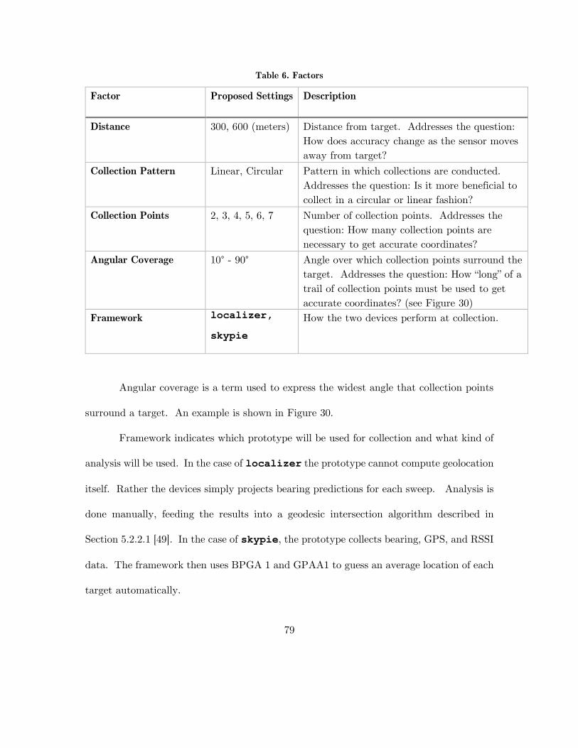
79
Table 6. Factors
Factor Proposed Settings Description
Distance 300, 600 (meters) Distance from target. Addresses the question:
How does accuracy change as the sensor moves
away from target?
Collection Pattern Linear, Circular Pattern in which collections are conducted.
Addresses the question: Is it more beneficial to
collect in a circular or linear fashion?
Collection Points 2, 3, 4, 5, 6, 7 Number of collection points. Addresses the
question: How many collection points are
necessary to get accurate coordinates?
Angular Coverage 10° - 90° Angle over which collection points surround the
target. Addresses the question: How “long” of a
trail of collection points must be used to get
accurate coordinates? (see Figure 30)
Framework localizer,
skypie
How the two devices perform at collection.
Angular coverage is a term used to express the widest angle that collection points
surround a target. An example is shown in Figure 30.
Framework indicates which prototype will be used for collection and what kind of
analysis will be used. In the case of localizer the prototype cannot compute geolocation
itself. Rather the devices simply projects bearing predictions for each sweep. Analysis is
done manually, feeding the results into a geodesic intersection algorithm described in
Section 5.2.2.1 [49]. In the case of skypie, the prototype collects bearing, GPS, and RSSI
data. The framework then uses BPGA 1 and GPAA1 to guess an average location of each
target automatically.
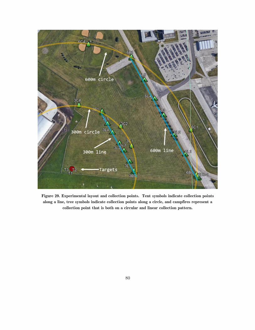
80
Figure 29. Experimental layout and collection points. Tent symbols indicate collection points
along a line, tree symbols indicate collection points along a circle, and campfires represent a
collection point that is both on a circular and linear collection pattern.
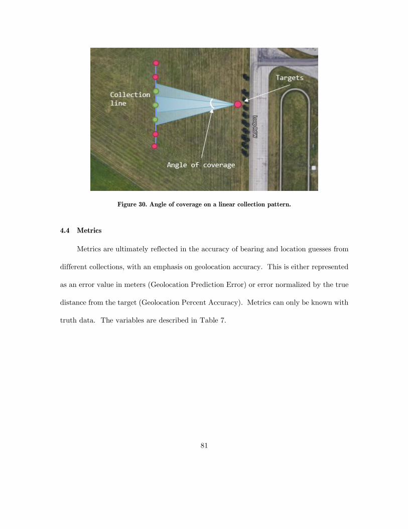
81
Figure 30. Angle of coverage on a linear collection pattern.
4.4 Metrics
Metrics are ultimately reflected in the accuracy of bearing and location guesses from
different collections, with an emphasis on geolocation accuracy. This is either represented
as an error value in meters (Geolocation Prediction Error) or error normalized by the true
distance from the target (Geolocation Percent Accuracy). Metrics can only be known with
truth data. The variables are described in Table 7.
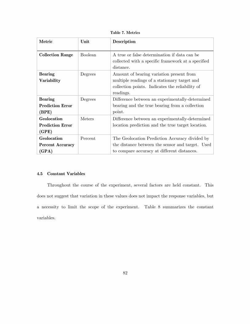
82
Table 7. Metrics
Metric Unit Description
Collection Range Boolean A true or false determination if data can be
collected with a specific framework at a specified
distance.
Bearing
Variability
Degrees Amount of bearing variation present from
multiple readings of a stationary target and
collection points. Indicates the reliability of
readings.
Bearing
Prediction Error
(BPE)
Degrees Difference between an experimentally-determined
bearing and the true bearing from a collection
point.
Geolocation
Prediction Error
(GPE)
Meters Difference between an experimentally-determined
location prediction and the true target location.
Geolocation
Percent Accuracy
(GPA)
Percent The Geolocation Prediction Accuracy divided by
the distance between the sensor and target. Used
to compare accuracy at different distances.
4.5 Constant Variables
Throughout the course of the experiment, several factors are held constant. This
does not suggest that variation in these values does not impact the response variables, but
a necessity to limit the scope of the experiment. Table 8 summarizes the constant
variables.

83
Table 8. Constant Variables
Factor Desired
Experiment Level
How Controlled? Anticipated Effects
Target locations Pre-defined layout
(see Figure 29)
Experimental design Varies
Number of Targets 3 Experimental design None
Target models LG Rebel 2 LTE,
ZTE ZFive 2 LTE
(x2)
Experimental design None
Traffic behavior WPA2 Access
Point
Device configuration Standardized
packet capture
distribution
Rotation rate 45 seconds per
revolution
Device configuration Slowed to increase
capture at longer
distances [41]
Channel hop interval 179 Time Units
(802.11 protocol),
about .183
seconds
Device configuration Most effective for
captures [41]
Channel hop distance 2 channels per
hop
Device configuration Most effective for
captures [41]
Initial bearing of sweep 0° (facing North) Manual check with
compass
Slight bearing
error introduction
[41]
Variables that need additional description are discussed here:
Target locations – are deployed as demonstrated in Figure 29. Targets are separated
enough to reduce interference from each other, but not enough to greatly vary their
general location from the collection points. The scale (targets along a 2 m line, <1%
of closest collection distance) would ideally reflect several Wi-Fi devices in a single
room. Targets sit atop a plastic folding table at different orientations as show in
Figure 31 and Figure 32.

84
Number of targets – the number is chosen to provide replicants for similar
measurements.
Target models – are chosen for cost efficiency. All are capable smartphones running
the same version of Android (6.0, Marshmallow).
Traffic behavior – as a Wi-Fi access point, beacon frames are expected roughly 10
times a second.
Rotation rate, Channel hop interval, and Channel hop distance are all chosen from
earlier research that suggests best packet capture rates [41].
Figure 31. Targets at target locations

85
Figure 32. Target orientations. Note each phone is oriented differently. Target 1 is propped up
horizontally using a cardboard box. To prevent Target 1 from blowing away, a partially full
water bottle is added to weigh it down while a Maroon 5 compact disk case kept the phone
pointed toward the collection points.
4.6 Uncontrolled Variables
As with most developed areas, the 2.4 GHz band is subject to wireless traffic outside
of the scope of the experiment from nearby devices. While this may cause interference,
this traffic simulates an environment in which the systems are designed to be operational.
A second uncontrollable variable is the inherent inaccuracy of GPS readings, which
are used in the field to establish target and collection locations. The error, potentially up
to 4.9 meters [50], is unavoidable unless using more precise measuring instruments.

86
4.7 Experimental Design
This section describes detailed instructions on how each experiment is conducted.
4.7.1 Geolocation Experiment: localizer
1. The same field location is used for all experiments.
2. Targets (cell phones) are placed on table at the target location specified in
Figure 29 in the configuration shown in Figure 31. The cell phones have their
Wi-Fi WNICs placed into AP mode.
3. The prototype is mounted on a stainless-steel support rack (0.78 m high)
strapped on top of a Ford F-150 truck (1.905 m), so that it rests a total of
2.685 m above the ground, which is a reasonable elevation for a low-flying
drone. A photo of the rig is shown in Figure 33, and details are shown in
Figure 34.
4. The prototype is turned on and connected to a laptop via Ethernet cord. The
laptop uses SSH to activate the localizer program. A separate directory is
made for each collection point to store data files. Collection parameters are
set to default, with the exception of sweep duration (set to 45 seconds)
5. The truck moves to the first collection point along a collection pattern, starting
at the southernmost point and moving north. The truck is placed in park and
remains stationary for collection.
6. An analog compass is used to manually move the antenna to 0° (magnetic
north).
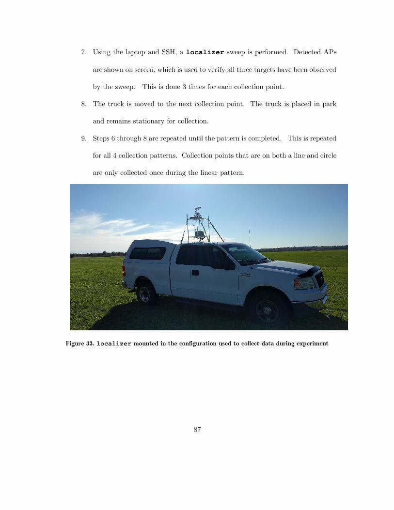
87
7. Using the laptop and SSH, a localizer sweep is performed. Detected APs
are shown on screen, which is used to verify all three targets have been observed
by the sweep. This is done 3 times for each collection point.
8. The truck is moved to the next collection point. The truck is placed in park
and remains stationary for collection.
9. Steps 6 through 8 are repeated until the pattern is completed. This is repeated
for all 4 collection patterns. Collection points that are on both a line and circle
are only collected once during the linear pattern.
Figure 33. localizer mounted in the configuration used to collect data during experiment

88
Figure 34. Detailed components of the mobilized localizer rig, which is secured to the truck
by ratchet straps
4.7.2 Bearing Variance Experiment: localizer
This experiment is done to analyze how much bearing readings differ from a
singular point at distances roughly 300 m and 600 m from the targets.
1. The field, targets, and truck are set up the same as Steps 1 through 4 in the
localizer Geolocation Experiment (see Section 4.7.1).
2. The truck is moved to point 3L2 shown in Figure 29. The truck is put in park
and remains stationary.

89
3. An analog compass is used to manually move the antenna to be facing to 0°
(magnetic north).
4. At least 10 sweeps are performed.
5. The truck is moved to point 6B1. The truck is put in park and remains
stationary.
6. Steps 3 and 4 are repeated for point 6B1.
4.7.3 Geolocation Experiment: skypie
In the skypie experiment, a subset of the localizer experiment is performed to validate
capture functionality and get initial feedback for the geolocation algorithms (BPGA and
GPAA).
1. The field, and targets are set up the same as Steps 1 through 3 in the
localizer Geolocation Experiment (see Section 4.7.1).
2. The truck is moved to the start of the 300 m collection line.
3. The skypie sensor payload is turned on. The skypie software is started
manually from the IDE using a keyboard and monitor, which are unplugged
after.
4. A driver moves the truck at a speed of roughly between 5 and 15 meters per
second (11 and 35 miles per hour), similar to the speed of commercial MUAVs
[2]. Meanwhile another individual handler holds skypie prototype out the
window and rotates it in slow circles using an unpredictable pattern. This was
done to resemble a drone operator performing erratic rotations.

90
5. The skypie program is turned off.
6. Step 4 is repeated for a second pass.
4.8 Summary
This chapter outlines the process and parameters under study in this research, as well
as details about how data collection occurs. The experimental environment is discussed
at length as well as metrics to judge effectiveness.

91
5. V. Results
5.1 Overview
This chapter describes results obtained from using the localizer and skypie
frameworks during the experiment described in Chapter 4.
Section 5.2 covers the localizer geolocation experiment. Because the localizer
prototype is designed for experimental use as opposed to operational use, it is the focus of
the statistical analysis. The relationship between the factors and the metrics are analyzed,
demonstrating best collection settings that can translate to any device performing
directional geolocation. Post-collection techniques and improvements are suggested in
Section 5.2.3.2.
The remainder of the chapter discusses results from using and developing the
operationally-oriented skypie. Section 5.3 demonstrates skypie’s collection
capabilities in the field and discusses the skypie geolocation experiment. Section 5.4
describes results of the skypie development process.
5.2 Geolocation Experiment: localizer
At each collection point shown in Figure 29, the localizer prototype took at least
3 separate readings to prevent having a single data point for each location. A reading
consists of a 360° sweep hopping 2 channels every 179 Time Units specified by the 802.11
protocol (about 0.183 seconds), which are the optimal configurations for beacon collection

92
under normal conditions [41]. The recommended sweep time is relaxed from 30 to 45
seconds because the distance is increased.
As bearing values are used to calculate geolocation predictions, this analysis starts
with a study of bearing prediction findings.
5.2.1 Bearing Prediction
In addition to the aforementioned tests, 10 additional sweeps are performed at a
solitary point along the 300 m and 600 m lines from the targets (see Section 4.7.2) to
investigate the variance in the bearing prediction given by localizer at these distances.
The results are depicted in Table 9. Note that point 3L2 is actually 261 m from targets
and point 6B1 is actually 599 m.
Table 9. Bearing predictions (in degrees) and variation from multiple sweeps at the same point
Point
Sample
Size Min Max Mean
Media
n
True
Bearing
Mean
Error
Media
n Error STD Variance
3L2 12 201 238 231.08 235 261.1 -30.02 -26.1 9.90 98.08
6B1 30 228 435 279.04 236.5 217.1 17.94 -24.6 64.27 4131.22
The amount of variance is significant, especially when proven later how much
bearing error can throw off a geolocation intersection. Accurate bearing is vital to getting
accurate results using intersection-based geolocation. Further inspection of the data
reveals two interesting features. The first is that both locations suffer from roughly the
same median bearing error (-25°) despite the distance and true angle from the targets.
Indeed, when all geolocation estimates are plotted, many data points in this experiment
seem to suffer from a systematic offset of -15 to -25 degrees. This pattern is shown in

93
Figure 35. Figure 36 visually examines three collection points and the offset of the
predicted target from the actual.
Figure 35. 300 m (light triangle symbols) and 600 m line (dark triangle symbols) geolocation
guesses.

94
Figure 36. Visual inspection of geolocation guesses demonstrating a possible systematic bearing
offset. The angles represent the difference between the true target bearing and bearing of the
proposed centered from three points on the 300 m line.
The second interesting feature is the distribution of bearing guesses at point 6B1
If the values are combined into a histogram (see Figure 37), it is notable that while the
majority of predictions are within 220° to 240° (the true direction of the target), a
secondary majority is found between 0° and 40°, for a difference of roughly 200°. Because
the offset for this spike is relatively close to 180°, it is likely this secondary spike is caused

95
by the back lobe of the directional antenna receiving signals when facing opposite the
targets. Note that the 300 m collection point does not suffer from this problem as shown
in Figure 38. It is likely errors like this are a function of distance and obstacles that cause
reflections.
Figure 37. Multiple bearing predictions at 600 m (point 6B1). Note the secondary majority
about 180 degrees out of phase with the primary majority.
Figure 38. Multiple bearing predictions at 300 m (point 3L2). Note that most data points are
within 9 degrees of each other.

96
It may benefit an advanced geolocation guessing algorithm to remove predictions
that fall into a secondary majority that are about 180° out of phase from a primary
majority. This can prevent geolocation guesses from being in the opposite direction of
the sensor if two such points are used as input. If only one input is in the wrong direction,
however, a geodesic intersection algorithm (similar to the one used in this research) still
theoretically returns a valid result because the Earth is (mostly) spherical. Points
calculated from two out-of-phase bearing predictions do interrupt geolocation averages.
In the case of a drone, the problem of removing these out-of-phase predictions is
made difficult because the true location is unknown and because the sensor is not
guaranteed a complete 360° rotation in a single location.
Lastly, overall bearing predictions are compared to the true values. This is shown
in box-and-whisker plot in Figure 39. Box-and-whisker plots in this research show
minimum and maximum as the whiskers while the box represents the 1st and 3rd quartiles.
The median is denoted by a line inside the box and average is denoted by an ‘x’. Outliers
appear dots outside the box.
Note again the median errors remain close to each other at -16.4° and -20° for 300
m measurements and 600 m measurements respectively, while outliers in the 600 m range
resemble back lobe misreadings.
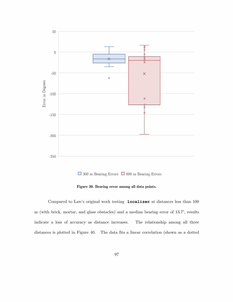
97
Figure 39. Bearing error among all data points.
Compared to Law’s original work testing localizer at distances less than 100
m (with brick, mortar, and glass obstacles) and a median bearing error of 13.7°, results
indicate a loss of accuracy as distance increases. The relationship among all three
distances is plotted in Figure 40. The data fits a linear correlation (shown as a dotted
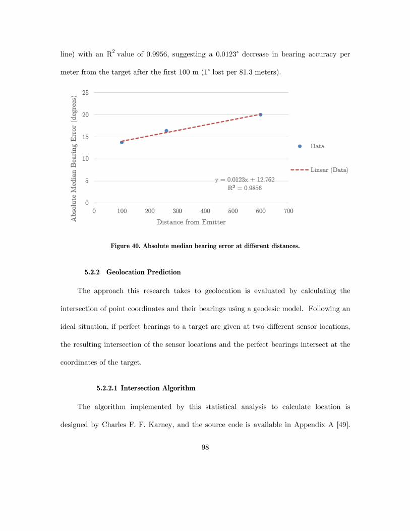
98
line) with an R2 value of 0.9956, suggesting a 0.0123° decrease in bearing accuracy per
meter from the target after the first 100 m (1° lost per 81.3 meters).
Figure 40. Absolute median bearing error at different distances.
5.2.2 Geolocation Prediction
The approach this research takes to geolocation is evaluated by calculating the
intersection of point coordinates and their bearings using a geodesic model. Following an
ideal situation, if perfect bearings to a target are given at two different sensor locations,
the resulting intersection of the sensor locations and the perfect bearings intersect at the
coordinates of the target.
5.2.2.1 Intersection Algorithm
The algorithm implemented by this statistical analysis to calculate location is
designed by Charles F. F. Karney, and the source code is available in Appendix A [49].

99
The algorithm finds the intersection of the two geodesics on the surface of the Earth. The
geodesics are created from the two coordinates and bearings the algorithm takes as input.
This is demonstrated visually in Figure 41.
Figure 41. Taking two collection point coordinates and a bearing from each, the algorithm
computes where the geodesics would intersect. This is the predicted location as computed by the
intersection algorithm.
To verify geolocation by calculating bearing intersection, Error! Reference source n
ot found. demonstrates what the predictions of all pairs along the 600 m line with a
prefect bearing (not the experimental result bearings). The top half of the figure shows
the entire field. Predictions are shown as white and black circles, which appear directly
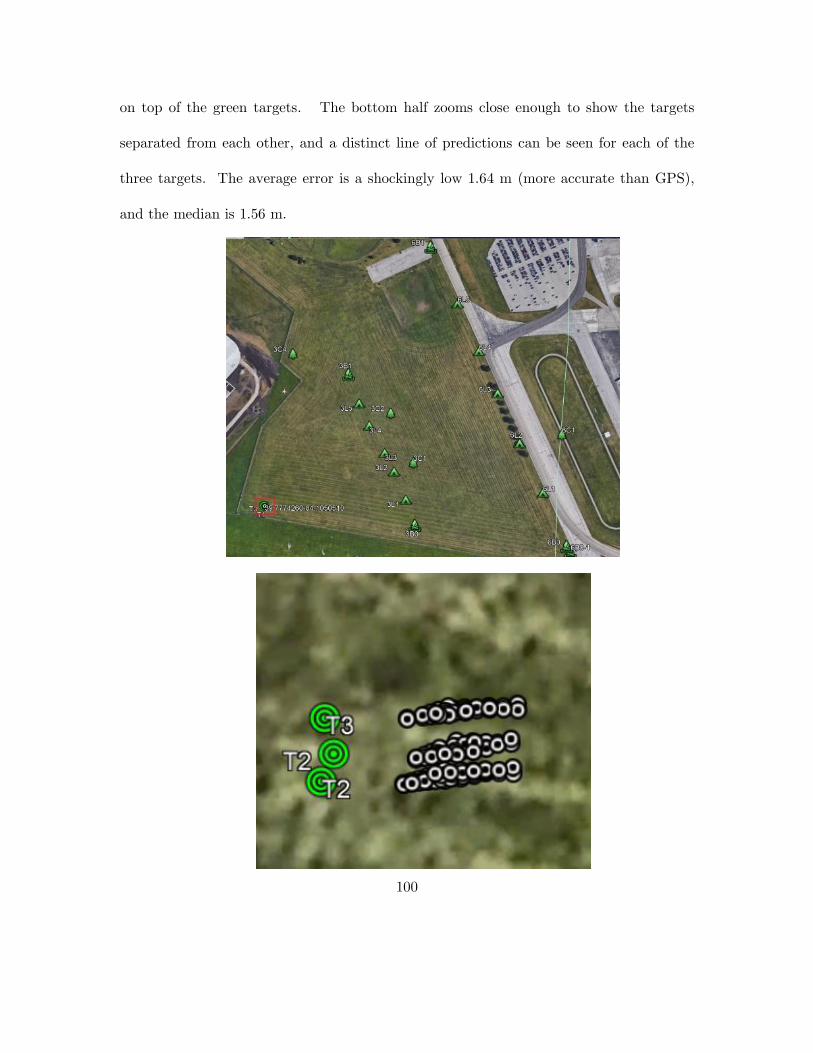
100
on top of the green targets. The bottom half zooms close enough to show the targets
separated from each other, and a distinct line of predictions can be seen for each of the
three targets. The average error is a shockingly low 1.64 m (more accurate than GPS),
and the median is 1.56 m.
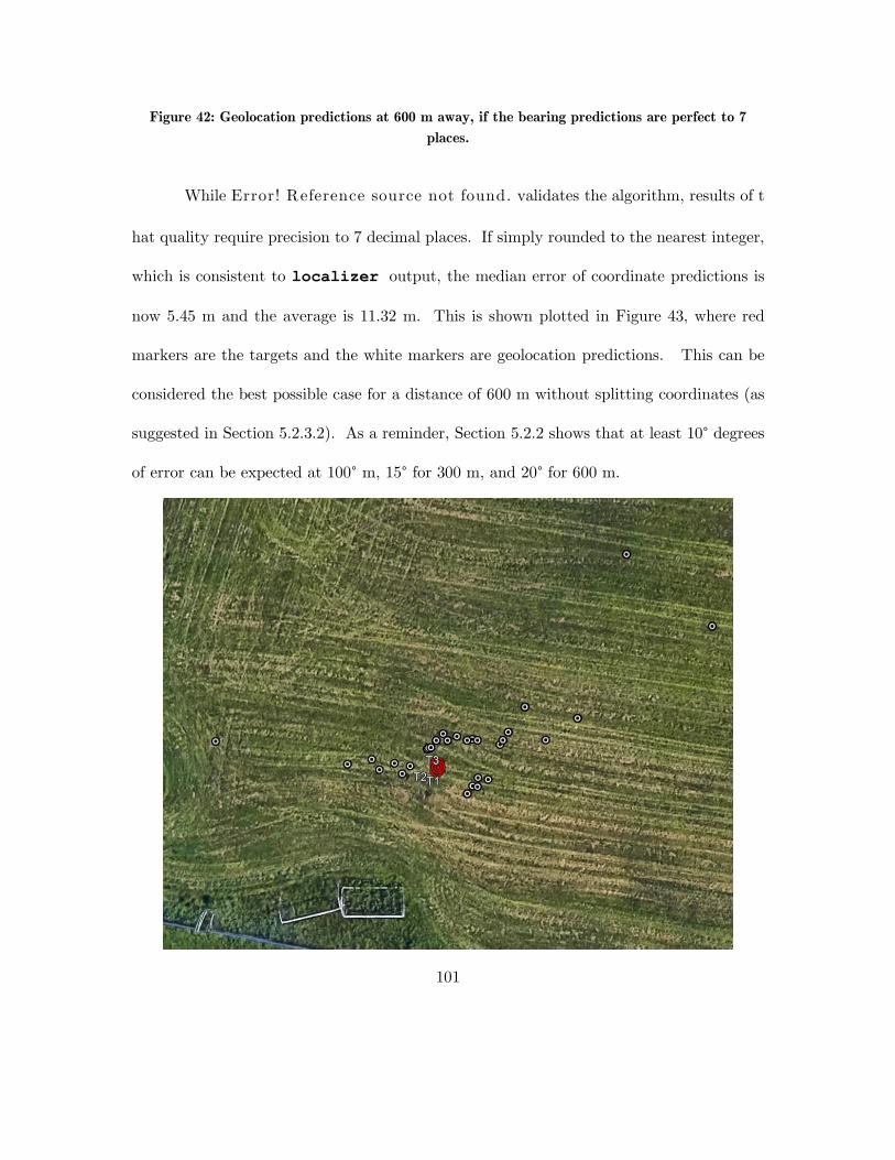
101
Figure 42: Geolocation predictions at 600 m away, if the bearing predictions are perfect to 7
places.
While Error! Reference source not found. validates the algorithm, results of t
hat quality require precision to 7 decimal places. If simply rounded to the nearest integer,
which is consistent to localizer output, the median error of coordinate predictions is
now 5.45 m and the average is 11.32 m. This is shown plotted in Figure 43, where red
markers are the targets and the white markers are geolocation predictions. This can be
considered the best possible case for a distance of 600 m without splitting coordinates (as
suggested in Section 5.2.3.2). As a reminder, Section 5.2.2 shows that at least 10° degrees
of error can be expected at 100° m, 15° for 300 m, and 20° for 600 m.

102
Figure 43. Geolocation predictions with perfect bearings, rounded to the nearest integer.
5.2.2.2 Raw Geolocation Estimates
In further calculations, geolocation predictions of over 3 km from the sensor are not
considered. Such predictions are considered inaccurate because conditions would have to
be exceptionally ideal for the directional antenna to pick up the signal. Without any other
outlier removal, Figure 44 shows an overview of the guesses among the difference collection
patterns and sizes.
Figure 44. All geolocation guesses by distance and collection pattern
Figure 45 shows the test field with most of the points plotted (those outside the
window are not shown). White markers indicate guesses from 300 m and red markers

103
indicates 600 m. Circle symbols represent guesses from the circle pattern and square
sybmols represent guesses from the line pattern. Overall, it seems predictions made at
300 m center around a point near the targets. A similar pattern can be seen for 600 m
predictions, but it is much less clear and many predictions are clearly wrong.
As found in previous research, a few of the outliers (caused by inaccurate bearings)
are so distant they make average location approaches inaccurate [41]. If the geolocation
algorithm is fortunate enough to be able to detect and remove outliers, accuracy can be
improved. This ability may be a luxury for data from a drone-mounted platform expected
to give real-time geolocation, but it could be possible with enough data from several data
collection locations.
Figure 45. Raw geolocation guesses plotted. White points indicate guesses from 300 m, red
indicates 600 m. Circle pins represent guesses from the circle pattern, square pins represent

104
guesses from the line pattern. The green line is a political boundary and is not part of the
experiment.
5.2.2.1 Outliers
The next sections continue investigation with outliers removed. Outliers cannot
simply be removed by Geolocation Prediction Error (GPE) because that involves truth
data, which a drone would not have in an operational setting. Instead, outliers are
considered guesses whose latitude or longitude fall outside 1.5 times the standard deviation
of the other guesses. If either latitude or longitude is an outlier, the guess is not included.
5.2.2.1 Distance
Normalized by distance from target, the closer distance of 300 m outperforms 600
m in median and average geolocation prediction error, and also has a tighter distribution.
Values are shown in Table 10 and represented in Figure 46.
Overall, median geolocation errors are off by at least a half of the distance from
the original target, while best-case guesses are 5%-10% for 300 m and 600 m respectively,
showing that geolocation via radiolocation can be extremely difficult to make accurate
within the expectation of GPS-quality results.
Table 10. Normalized Geolocation Error vs. Distance
300 m 600 m
Average 49% 64%
Median 46% 62%
Standard Deviation 19% 26%

105
Figure 46. Distance vs. Normalized Geolocation Error
5.2.2.2 Collection Pattern
Figure 47 shows the collection pattern mapped at each distance. At 300 m, results
indicate geolocation prediction improves when the collection is done by a circular pattern.
At 600 m, it appears the distinction is less pronounced and a circular pattern is less
accurate. This is hard to determine with confidence due to the missing data point at 6C3.
To further explore if there is a difference between collection pattern, Figure 48 shows
the results when both line and circle collection cover 68° and use 4 equally-spaced collection
points {Line = (3B0, 3L2, 3L4, 3B1), Circle = {3B0, 3C1, 3C2, 3B1}}. Here, the points

106
are essentially the same with the circular points being slightly farther away (but on the
same azimuth from the target). While the quartiles appear to make the circular pattern
look more accurate, the median errors are relatively close at 9.77 m apart. Table 11
shows the results for 600 m as well under similar parameters. In summary, it cannot be
certain if difference is caused primarily by collection pattern.
Figure 47. Collection pattern normalized by distance (angular coverage varies)

107
Figure 48. Geolocation error among collection pattern at 300 m (same angular coverage)
Table 11. Collection Pattern Errors
Pattern Line
(300 m)
Circle
(300 m)
Line
(600 m)
Circle
(600 m)
Points 4 4 4 3
Angular
Coverage
68° 68° 68° 68°
Guesses 32 34 39 30
Average 47.34% 39.69% 63.73% 67.75%
Median 44.38% 41.12% 61.11% 77.16%

108
5.2.2.3 Angular Coverage
The relationship between the angle of coverage as illustrated in Figure 30 and
bearing error is represented in the scatter plot in Figure 49, where error is normalized over
the distance from the target. Overall, increasing angular coverage decreases bearing error.
The most significant decrease in error occurs by increasing coverage from 10° to 30°.
More predictions exist for lower coverage angles because there are more points to
compare against at smaller angles than larger ones. There exists a large disparity between
predictions for a single angular value, which indicates that both “good” and “bad” guesses
can come from small and large angles alike. “Bad” guesses are more likely to happen at
values at very low coverage (those less than 25°). Notably, “good” guesses at low angles
are relatively comparable to “good” guesses at large angles, suggesting quality bearing
readings could still produce quality predictions from smaller angles.
Trends from both distances show that increasing coverage from 10° to 30° decreases
error the most. Improving the coverage between 45° and 65° did not improve error by any
recognizable amount. The lowest median errors are at 32° and 87°.
To further show the distributions among similar angles, Figure 51 shows a
breakdown of box-and-whisker plot of guesses for every set of points at 600 m.

109
Figure 49. Angular Coverage between 2-Sample Geolocation Guesses at 300 m
Figure 50. Angular Coverage between 2-Sample Geolocation Guesses at 600 m

110
Figure 51. Angular coverage box-and-whisker plot shows distribution of angular coverage at 600
m.
5.2.2.4 Collection Path Length and Number of Collections
The next investigation is the number of adjacent points that are needed to get the
most error reduction. The real-world application of this is to determine how far (relative
to target distance) and how many 360° collections a drone needs to perform get the best
geolocation prediction.
Figure 52 plots average predictions errors for groups of predictions. The groups are
composed of subsequent points along a collection pattern. The more points a group has,
the larger its dot is, with the smallest groups made of 2 data points and the largest having
7. The location on the x-axis of a dot indicates total length of collection the group
represents. A reasonable assumption is that as a collection group increases in length and

111
number of points, error should decrease, which would be represented as dots getting lower
as they increase in size or move to the right.
Whereas there is a discernable correlation at 300 m (shown by the dashed trendline
in Figure 52), there is hardly any correlation at 600 m, shown in Figure 53. It seems
increasing collection points and length at this distance yields little benefit. This can be
seen when the predictions are plotted on a map (Figure 54); most bearing estimates are
prone to intersecting too far in front or behind the target, creating a pattern sweeping
around the true locations.
Figure 52. Length of collection vs. average error at 300 m. Generally, as collection length
increases and points increase, error decreases.
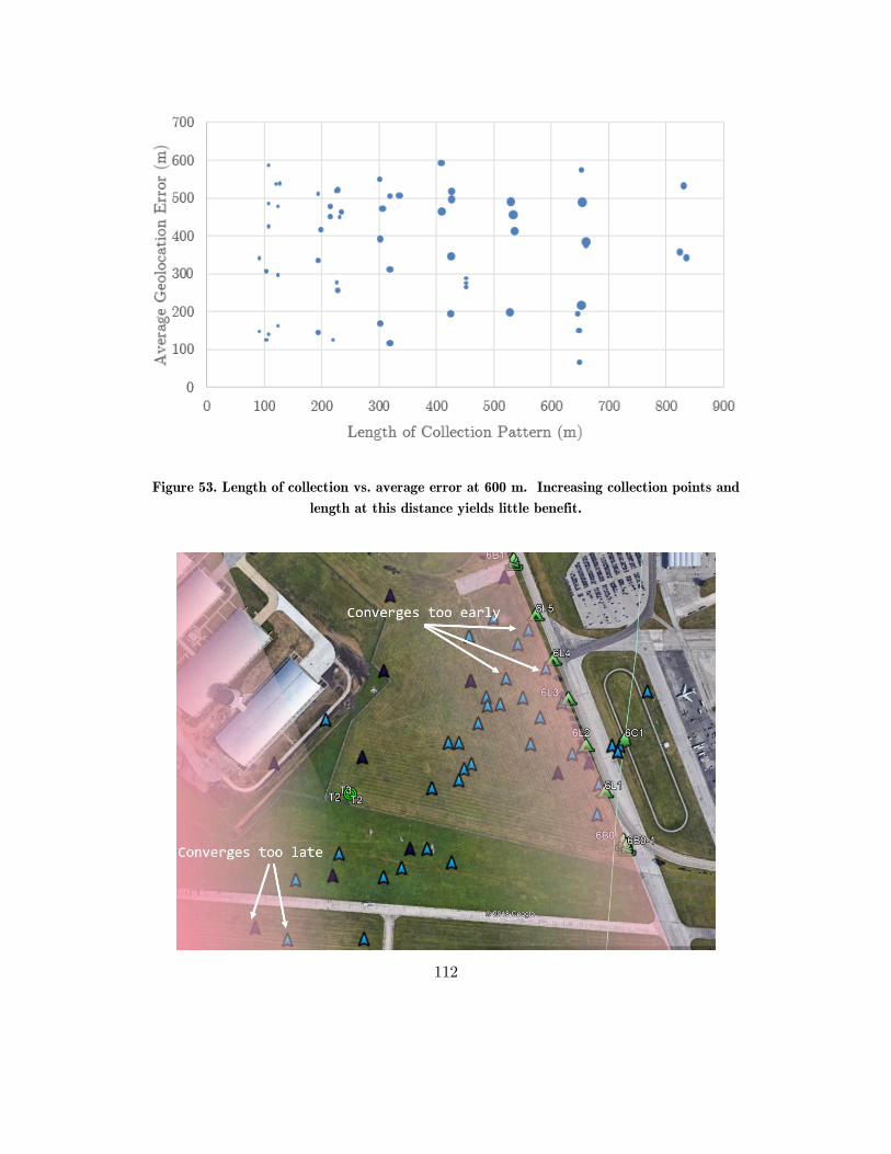
112
Figure 53. Length of collection vs. average error at 600 m. Increasing collection points and
length at this distance yields little benefit.
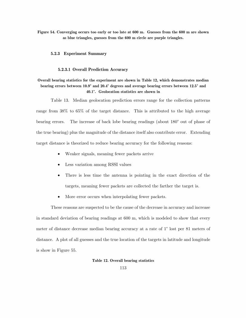
113
Figure 54. Converging occurs too early or too late at 600 m. Guesses from the 600 m are shown
as blue triangles, guesses from the 600 m circle are purple triangles.
5.2.3 Experiment Summary
5.2.3.1 Overall Prediction Accuracy
Overall bearing statistics for the experiment are shown in Table 12, which demonstrates median
bearing errors between 10.9° and 20.4° degrees and average bearing errors between 12.5° and
40.1°. Geolocation statistics are shown in
Table 13. Median geolocation prediction errors range for the collection patterns
range from 38% to 65% of the target distance. This is attributed to the high average
bearing errors. The increase of back lobe bearing readings (about 180° out of phase of
the true bearing) plus the magnitude of the distance itself also contribute error. Extending
target distance is theorized to reduce bearing accuracy for the following reasons:
Weaker signals, meaning fewer packets arrive
Less variation among RSSI values
There is less time the antenna is pointing in the exact direction of the
targets, meaning fewer packets are collected the farther the target is.
More error occurs when interpolating fewer packets.
These reasons are suspected to be the cause of the decrease in accuracy and increase
in standard deviation of bearing readings at 600 m, which is modeled to show that every
meter of distance decrease median bearing accuracy at a rate of 1° lost per 81 meters of
distance. A plot of all guesses and the true location of the targets in latitude and longitude
is show in Figure 55.
Table 12. Overall bearing statistics

114
300 Circle 300 Line 600 Circle 600 Line
Bearing Samples 76 44 22 74
Average Bearing Error -18.92 -12.48 -29.82 -46.19
Median Bearing Error -18.67 -15.05 -10.87 -20.40
Table 13. Overall geolocation statistics
Distance and Pattern 300 Circle 300 Line 600 Circle 600 Line
Average Prediction Error 112.53 156.58 317.30 388.65
Median Prediction Error 121.38 141.36 342.09 399.36
% Median Error 38% 52% 53% 65%
% Average Error 40% 24% 57% 67%
Figure 55. Plot of all location predictions. The three targets appear as one at this scale.

115
5.2.3.2 Prediction Improvements
Methods of analysis so far have taken predictions as a pair of coordinates and the
resulting distance error from the target. This is useful for examining which parameters
and trends to deliver more accurate guesses, but it requires truth data and is not the most
accurate strategy, as this section will show.
This next section covers the construction of predictions without knowing the true
target location while at the same time using a simple technique to reduce error.
Re-inspection of Figure 43 shows that even when bearing predictions are correct to
the single digit, the average distance from the target of each prediction increases around
the target, with few landing on the target itself. However, when latitudes and longitudes
are separated and the centroid or medoid are taken for each, then recombined into a new
coordinate, the result is a better reflection of target location than if done so as coordinate
pairs.
Applying this simple strategy to the experiment results, the predictions fall to a
more reasonable error rate.
An approach using the median and averaging of coordinates separately is shown in
Table 14 and Table 15 respectively. Averaging latitudes and longitudes separately is
shown to be the best method for reducing error across most sets, capable of getting
predictions under 86 meters for three of the four sets (two at 300 meters and one at 600).
The fourth set (600 m line) suffered from excessive bearing inaccuracy and back lobe
readings that continued to throw both the average and median off.

116
To show experiment results, Figure 56 shows all predictions and the average and
median coordinates on the 300 m line. Figure 57 shows the same for the 300 m circle,
Figure 58 for the 600 m line, and Figure 59 for the 600 m circle. Figure 60 shows the field
from a tilted perspective with all collections combined. The green line is a political
boundary and is irrelevant to this research.
Table 14. Separated coordinate median approach
Distance and Pattern 300 Circle 300 Line 600 Circle 600 Line
Median Latitude 39.776798 39.77666 39.777823 39.77822
Median Longitude -84.10427 -84.1044 -84.1042 -84.10143
Median Coord Error 97 101 84 321
% Median Coord Error 32% 34% 14% 54%
Table 15. Separated coordinate average approach
Distance and Pattern 300 Circle 300 Line 600 Circle 600 Line
Average Latitude 39.776985 39.77679 39.77772 39.778366
Average Longitude -84.10445 -84.1045 -84.10425 -84.10136
Average Coord Error 70.1 85.2 76 333.1
% Average Coord Error 23% 28% 13% 56%

117
Figure 56. Guesses, median (red ‘M’ marker), and average (orange ‘A’ marker) coordinate
predictions on 300 m line using centroid calculations

118
Figure 57. Guesses, median, and average coordinate predictions on 300 m circle using centroid
calculations

119
Figure 58. Guesses, median, and average coordinate predictions on 600 m line using centroid
calculations

120
Figure 59. Guesses, median, and average coordinate predictions on 600 m circle using centroid
calculations
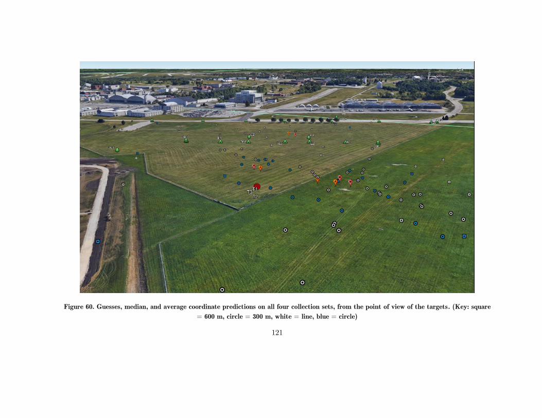
121
Figure 60. Guesses, median, and average coordinate predictions on all four collection sets, from the point of view of the targets. (Key: square
= 600 m, circle = 300 m, white = line, blue = circle)

122
5.3 Geolocation Experiment: skypie
A subset of the localizer experiment is run on the skypie framework to
demonstrate capture functionality in the field and provide initial feedback for the
geolocation algorithms (BPGA1 and GPAA1). The collection pattern chosen is the 300
m line, as described in Section 4.7.3.
The telemetry and packet captures are processed through Bearing Prediction and
Geolocation Algorithm 1 (BPGA1) and Geolocation Predication Averaging Algorithm 1
(GPAA1) using skyport. Figure 61 shows the telemetry history of the sensor as seen
from the Sensor App, and Figure 62 shows the computed geolocation predictions from the
Analysis App.
skypie is also capable of successfully collecting from all targets at the 600 m line,
but analysis suffered the same problems as 300 m.

123
Figure 61. skyport telemetry history of the skypie on the 300 m line test, with the purple
lines indicating the direction the sensor is facing at the time. The red dot indicates the location
of the targets.
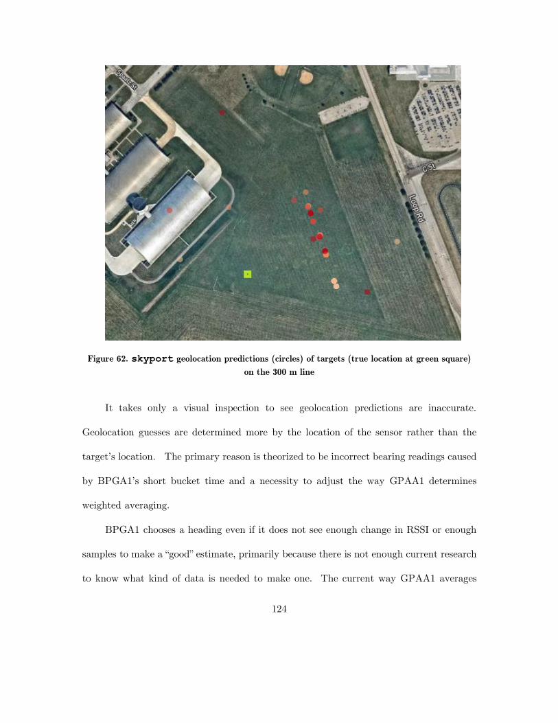
124
Figure 62. skyport geolocation predictions (circles) of targets (true location at green square)
on the 300 m line
It takes only a visual inspection to see geolocation predictions are inaccurate.
Geolocation guesses are determined more by the location of the sensor rather than the
target’s location. The primary reason is theorized to be incorrect bearing readings caused
by BPGA1’s short bucket time and a necessity to adjust the way GPAA1 determines
weighted averaging.
BPGA1 chooses a heading even if it does not see enough change in RSSI or enough
samples to make a “good” estimate, primarily because there is not enough current research
to know what kind of data is needed to make one. The current way GPAA1 averages

125
these guesses is also not sufficient to determine which predictions to apply more weight.
The result is that many incorrect bearings converge much too quickly, causing predictions
to be very close to where the antenna is facing. Improvement for these algorithms based
upon this trial data is in Section 6.2.2.
5.4 skypie Framework Developments Results
This section discusses results and lessons learning from development of the skypie
prototype.
5.4.1 Hardware Design Decisions and Rationale
The next section discusses several design choices that are made after initial research,
experimentation, or pilot tests.
I. Stationary vs. Rotating Antenna. A stationary antenna is chosen because the
magnetic interference from a stepper motor would greatly interrupt any
magnometer/compass readings, thus making heading measurements inaccurate.
Pilot tests with a stepper motor greatly impacted the analog compass during pilot
tests with the localizer prototype.
II. Smartphone vs. Raspberry Pi Computer. The use of a cellular device as the main
computer was considered, but ultimately decided against. The benefit is that
cellphones have a slim form factor, good computing specifications, light-weight
batteries, built-in cellular connectivity, and also come with many sensors needed
for geolocation. However, cellphones lack the input/output ports that the
Raspberry Pi offers (four USB, Ethernet, and GPIO pins), have a higher cost, and

126
less operating system choices, so the Raspberry Pi is chosen as the main computing
platform.
III. Drone Dependence vs. Drone Independence. Deciding the amount of dependency
on a drone is a difficult choice for designing the payload. On one hand, payload
integrated into the drone has the advantages of on-board sensor data (camera feeds,
GPS feeds), communication channel, and potentially a power source. While several
custom and open-source drone protocols exists, most commercial drones have
propriety protocols, meaning the payload would be pigeonholed into a specific make
or manufacturer.
IV. Raspbian vs. Kali Linux. The two operating systems considered for use on the
sensor platform are Raspbian and Kali Linux. Raspbian is a variant of the Debian
OS made by the Raspberry Pi corporation specifically for operability on Raspberry
Pi chips, so it provides a larger support ecosystem. This includes utilities and
libraries useful with the hardware components. Kali Linux is also a variant of
Debian used for penetration testing and CAN, and comes pre-loaded with many
hacker utilities and programs. Raspbian supports the necessary Python libraries
for performing collection and analysis functions required by localizer (originally
developed for Raspbian) and skypie. Setup with Raspberry Pi hardware, such
as the Sense HAT, is much easier with Raspbian.
While the payload is designed to focus on having cyber-attack capabilities,
the ultimate goal is to mimic and pass through a connection from the attacker’s
computer as if it is local (this scheme is described in 6.5). This gives the hacker

127
more flexibility and the payload operating system does not need excessive hacker
tools itself.
V. Cellular vs. Radio Reachback. A cellular connection is beneficial in urban areas
where the cellular infrastructure exists. The attacker also has the advantage of
communicating with the device from larger distances since the cellular networks
allow Internet data connections. From a stealth standpoint, in urban environments
cellular signals are ubiquitous and it may be harder for a defender to identify the
link. A radio communication channel is better in environments with poor or no
cellular service, however the attacker needs to be within radio range of the sensor.
Commercial radio chips also come in a limited amount of frequencies, which an
astute defender may be able detect. For this research, a cellular connection is
chosen to mimic a scenario where the attacker is targeting a home or business.
5.4.2 skypie Framework Functionality
Table 16 provides a list of features that were planned and completed in this
iteration of research and suggests steps that could be taken to improve it in the future.
The symbols in the ‘State’ column indicate the progress of each feature. A green circle
indicates the feature is completed, a yellow triangle indicates the feature is implemented
but should be improved, and a red diamond indicates the feature is not implemented.

128
Table 16. skypie Current Features and Future Work
Category Feature Implementation Status State Next Step
Wi-Fi Passive Wi-Fi Sniffing Proven Operational Complete
Wi-Fi Bearing Prediction
Rudementary algorithm
(BPGA1) Improve accuracy
Wi-Fi Geolocation Prediction
Rudementary algorithm
(GPAA1) Improve accuracy
Wi-Fi Device Analysis Rudementary identification
Add features (see
CNA/CNE category)
Wi-Fi Access Point Interaction
Present in locazlier, not
skypie Implement
UI Web UI Suite Proven Operational Optimize graphing speeds
UI Satelite Imagary Analysis Proven Operational Complete
Telemetry GPS Sensor Proven Operational Complete
Telemetry Accelerometer Operational Improve accuracy
Operational Database Storage Structure Proven Operational Complete
Operational Data Upload
Works over secondary
WLAN interface Celluar Implementation
Operational Data Download
Works over secondary
WLAN interface Celluar Implementation
Operational Secure data transfer SFTP connection Complete
Operational Operation Battery Life
4+ hours while collecting
Wi-Fi Sufficient
Operational Remote Sensor Control Proven Operational Complete
Operational Remote Sensor Geolocation Proven Operational Complete
Operational
Arbitrary Remote
Command Execution Proven Operational Complete
Operational
Multi-Sensor Capability
and Data Fusion Proven Operational Test with multiple sensors
Operational Survivable Chasis Proven Operational Make water-resistant
CNA/CNE EAPOL Packet Grabbing Stub Implement
CNA/CNE Mirror Mode Stub Implement
CNA/CNE Associated Client Tracking Stub Implement
CNA/CNE Probe Request Tracking Stub Implement
Bluetooth Passive Sniffing Stub Add hardware, implement

129
6. VI. Conclusion and Future Work
6.1 Overview
This chapter summarizes the research and results found during development and
experimental evaluations. Section 6.2 reiterates notable conclusions from experimentation
and statistical analysis. Section 6.3 synthesizes findings in the context of cybersecurity
and privacy. Section 6.4 discusses potential countermeasures. Lastly, Section 6.5 provides
possibilities for future work in the field of cyber-attack drones.
This research succeeds in proving the hypothesis that a functional cyber-attack drone
payload could be built under $500, under 1 kg, and within four months. One of the four
data sets shows that geolocation via radiolocation of Wi-Fi targets can be accurate below
the hypothesized 15% of distance from the targets at 600 m using less than 90° of angular
coverage and full channel hopping, however the other three data sets failed to reach that
degree of accuracy. Geolocation efforts with larger coverage angles, targeted single-channel
sweeps, and intelligent filtering are recommended to increase accuracy.
The research goals, which are to investigate the effectiveness of geolocation via
radiolocation and implement an attack drone payload are both met.
6.2 Research Conclusions
6.2.1 Geolocation via Radiolocation Conclusions
Geolocation via 802.11 emissions (Wi-Fi) using a portable directional antenna is
possible, but difficult to achieve the accuracy that GPS delivers. This research found that
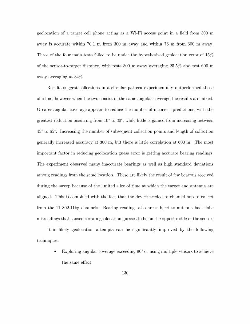
130
geolocation of a target cell phone acting as a Wi-Fi access point in a field from 300 m
away is accurate within 70.1 m from 300 m away and within 76 m from 600 m away.
Three of the four main tests failed to be under the hypothesized geolocation error of 15%
of the sensor-to-target distance, with tests 300 m away averaging 25.5% and test 600 m
away averaging at 34%.
Results suggest collections in a circular pattern experimentally outperformed those
of a line, however when the two consist of the same angular coverage the results are mixed.
Greater angular coverage appears to reduce the number of incorrect predictions, with the
greatest reduction occurring from 10° to 30°, while little is gained from increasing between
45° to 65°. Increasing the number of subsequent collection points and length of collection
generally increased accuracy at 300 m, but there is little correlation at 600 m. The most
important factor in reducing geolocation guess error is getting accurate bearing readings.
The experiment observed many inaccurate bearings as well as high standard deviations
among readings from the same location. These are likely the result of few beacons received
during the sweep because of the limited slice of time at which the target and antenna are
aligned. This is combined with the fact that the device needed to channel hop to collect
from the 11 802.11bg channels. Bearing readings also are subject to antenna back lobe
misreadings that caused certain geolocation guesses to be on the opposite side of the sensor.
It is likely geolocation attempts can be significantly improved by the following
techniques:
Exploring angular coverage exceeding 90° or using multiple sensors to achieve
the same effect

131
Intelligently filtering back lobe readings
Filtering outlier geolocation predictions intelligently
Performing full 360° sweeps on the 802.11 channel of the target
6.2.2 BPGA1 and GPAA1 Conclusions
Testing the skypie framework enacted a test of the BPGA1 and GPAA1 algorithms,
which generally failed in accuracy. GPAA1 failed because BPGA1 surmised predictions
from too many incorrect bearing readings. BPGA1 make geolocation guesses without
enough data. BPGA1 can be improved by adding additional weight on RSSI values as
opposed to just weight based on geographic separation.
Both algorithms are time-based, where they issue a prediction at the end of every
time interval, even if the guess is inaccurate. Both algorithms could be improved by only
fielding guesses that meet a proven threshold, such as only returning a bearing if the RSSI
values have seen a spike in power while the accelerometer indicates a minimum threshold
of rotation. Buckets in which there is not enough data means the algorithm should wait
for more information.
In the future, the algorithms could also gain information from other telemetry fields
available in the implementation, such as GPS azimuth and GPS speed.
6.3 Research Significance and Synthesis
Developing the skypie prototype and testing geolocation with the localizer
prototype gave insight into challenges with precise geolocation and device tracking from
long distances by only using Wi-Fi signals.

132
At the observed error rates, distances, and experimental constraints, tracking a
victim’s cell phone as they walked through the city would be inaccurate, most likely
showing dots in many places the device never was. Averaging would most likely yield a
location in the vicinity. Trying to track the person as they moved would also be
challenging, as predictions are so scattered when the device is stationary it is hard to tell
the difference as to if the device is actually moving or just experiencing variation in guesses.
This research found several techniques to lower overall error (see Section 6.2.1), but
overcoming the underlying obstacles—getting accurate bearing readings and a mature
geolocation algorithm—requires more work on the part of an attacker to get precise and
accurate results.
That said, even with error rates in the 30% range, a wireless attack payload can
easily still perform cyber operations on a target, to include sniffing, injecting, and
performing denial-of-service attacks. These are activities an attack framework like
skypie can perform from 600 m away. This is significant because a motivated attacker
can also perform these attacks with less than $500, purely open source software, a
commercial drone—all while acting from a remote location and remaining anonymous. If
the drone becomes captured, the attacker can evade detection by remotely self-destructing
the payload’s operating system (a bonus feature in skypie). If the communication
channel is similar to that of skypie, there would not be a clear data trail to follow since
the payload only contacts a proxy SFTP server and the cellular SIM card can be bought
with cash.

133
Indeed, like the drones in Bioshock, a well-crafted cyber-attack drone poses a
significant threat to an unsuspecting target.
6.4 Countermeasures
During the development of a wireless cyber-attack attack platform and experiments
testing radiolocation using Wi-Fi signals, several countermeasures have been identified
that would make conducting CNA and CNE more challenging in this field:
1. Random and Rotating MAC Addresses. Device profiling can be done easily
if MAC addresses remains constant. Using MAC addresses is also convenient
because it still works in the presence of most encryption schemes. If the MAC
of a device changes often, the attacker must resort to more complicated forms
of identification (such as radio frequency fingerprints or behavior correlation).
2. Wi-Fi PSK Changes and Unique SSIDs. Each time the PSK changes, an
attacker needs to re-capture an EAPOL/WPA2 handshake and crack the
password for that network. Changing the PSK periodically may deter an
attacker who has previously compromised a network. Unique SSIDs prevent
the password from being cracked quickly by a rainbow table.
3. Disable Probe Requests in Future Protocols. Probe requests reveal unique
connection history about a device, revealing associations with previous SSIDs.
Since SSIDs do not change often and location information about them can be
found online [28], probe requests can also leak geolocation history.

134
4. Varying AP Signal Strength. Radiolocation discussed in this work relies
inherently on RSSI. If an AP were to randomly alter signal intensity, even
slightly, amplitude-based geolocation would lose accuracy.
6.5 Future Work
Creating, developing, and forging the technology cyber-attack drone has many
avenues for improvement. Several suggestions, particularly those that build upon
radiolocation techniques and the foundational skypie framework built in this research
are:
1. Bearing Prediction. Decreasing bearing prediction error is the most
straightforward way to increase geolocation accuracy. This task is
complicated by the fact that the sensor is both moving in space and rotating
unpredictably—making determining a target’s heading difficult to impossible
if there is not enough rotation in a particular location. Additionally, the
sensor is designed to be on an airborne MUAV that has lift and steering
generated by electromagnetic motors. Overcoming these challenges is
important for improving this type of radiolocation.
2. Geolocation Algorithm. Intelligently identifying how to combine multiple
predictions with different confidence levels would also improve geolocation
accuracy. This requires more experimental geolocation collection and
alteration of how sensor data is combined into a final guess. Additional
telemetry fields available from the GPS module, such as GPS speed and

135
azimuth, may be beneficial to utilize in new algorithms. Additionally, a
higher-level algorithm may be able to assess patterns from lower-level
algorithm to make more informed guesses. An example of this potential is
shown in Figure 63 (the experiment results from Section 5.2.3), where rays
have been drawn where geolocation guesses seem to form lines. One of these
intersections occurs at the exact location of the targets. If a higher-level
algorithm does a similar analysis, it might be able to identify guesses beyond
simple averaging. This would be beneficial in environments with obstacles.
Figure 63. All geolocation guesses from the localizer experiment. After adding secondary
rays (pink lines) along trend lines, this plot begs the question: “is the truth out there?”

136
3. Airborne Operation Performance. Putting and testing the payload for
operations on an actual drone is an inevitable step in this research. The
added elevation from the drone has been shown to increase signal reception
in pilot studies, and it is possible bearing and geolocation predictions would
improve as well. Additional environmental challenges may arise, however
the skypie successfully can be used in bumpy setting without significant
issues (it was tested on motorized mountain bicycle on a bumpy field).
4. Additional Wireless Protocols. Now that a software framework and
prototype exists for collecting, transporting, and viewing Wi-Fi traffic,
adding sensors and support for other protocols is a natural choice. Adding
Bluetooth and Software Defined Radio (specifically GSM) sensors expands
the attack surface to the majority of networked consumer wireless devices
with little weight addition.
5. CNA and CNE Features. The development of skypie ends right at an
exciting point—where an existing framework exists and higher-level wireless
CNA/CNE features are ready to be built in. These can include, but are not
limited to: connection association correlation, probe request correlation,
advanced device profiling, EAPOL/WPA2 sniffing and cracking, denial of
service attacks, replay attacks, and interactive AP connections.
A proposed feature for the skypie framework is ‘Mirror Mode,’ which
would allow an attacker to theoretically trick a victim AP into thinking the
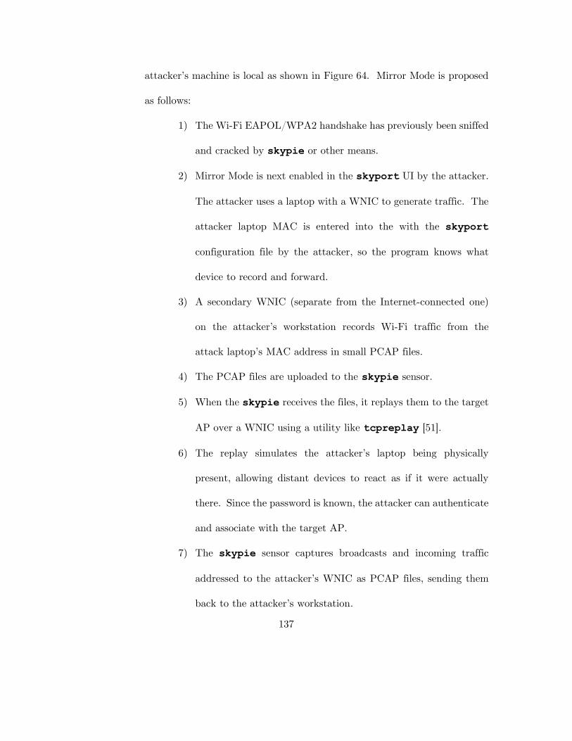
137
attacker’s machine is local as shown in Figure 64. Mirror Mode is proposed
as follows:
1) The Wi-Fi EAPOL/WPA2 handshake has previously been sniffed
and cracked by skypie or other means.
2) Mirror Mode is next enabled in the skyport UI by the attacker.
The attacker uses a laptop with a WNIC to generate traffic. The
attacker laptop MAC is entered into the with the skyport
configuration file by the attacker, so the program knows what
device to record and forward.
3) A secondary WNIC (separate from the Internet-connected one)
on the attacker’s workstation records Wi-Fi traffic from the
attack laptop’s MAC address in small PCAP files.
4) The PCAP files are uploaded to the skypie sensor.
5) When the skypie receives the files, it replays them to the target
AP over a WNIC using a utility like tcpreplay [51].
6) The replay simulates the attacker’s laptop being physically
present, allowing distant devices to react as if it were actually
there. Since the password is known, the attacker can authenticate
and associate with the target AP.
7) The skypie sensor captures broadcasts and incoming traffic
addressed to the attacker’s WNIC as PCAP files, sending them
back to the attacker’s workstation.
138
8) The attacker’s workstation replays the PCAPs back over its
WNIC connection, playing the traffic back to the attacker’s
laptop.
There no doubt latency will be introduced by Mirror Mode, but if
successful, the attacker then has the advantage of attacking from ‘inside’ the
private wireless network remotely, successfully gaining Remote Physical
Proximity (RPP). This would be a new type of injection attack that
combines the ease and anonymity of remote attacks with the inherent
weaknesses wireless traffic.

139
Figure 64. Conception description of ‘Mirror Mode,’ a theoretical and powerful feature that could be implemented with the skypie
framework

140
Appendix A. Supplemental skypie Design Resources
These resources are provided to add clarity on specifics of certain aspects of the
skypie/skyport framework design.
A.1 skypie/skyport Data Storage Scheme
The framework’s data storage scheme is shown in Figure 65. Boxes indicate
directories, and files inside are shown next to or below each box as text.
The left column represents the attacker’s workstation, which is running skyport.
Data is stored in the ./skyport/database/sensors directory, with a subdirectory
for each sensor. In the example depicted in Figure 65, there are three sensors deployed,
“starchy,” “gunter,” and “xena.”
Directories in green are downloaded from the skypie sensor, which is depicted in
the right column. Directories that are purple are uploaded to the skypie sensor.
Directories in blue do not move.
The center column depicts the SFTP server, which acts as an Internet-facing
intermediary for the sensor and the attacker’s workstation. The files in the “synch”
directory of each sensor are uploaded here until the attacker downloads them.

141
Figure 65. skypie/skyport data storage scheme
A.2 skypie Default Configuration File (config.txt)
The program utilizes a standard configuration file scheme similar to Microsoft
Windows INI files, consisting of sections and key-value pairs. This default file is
commented to describe each setting. If the program expects a certain set of values, those
values are printed in brackets after the description in the comments. For example, the
logging_level key in the [log] section accepts values that are ‘debug’, ‘info’,
‘warning’, ‘critical’ or ‘none’.
## Skypie Config File. Modifying this file alters the behavior of the program. # SFTP Server [fileserver] # Sensor's name, creates unique storage location on skyport. Useful for multiple sensors. name=starchy # Credentials for the SFTP account of the sensor's name

142
verifier=aSecretPassword9000 # Port to connect over SFTP for uploading/downloading sensor data sftp_port=2222 # IP/hostname to connect over SFTP for uploading/downloading sensor data sftp_server=ftp.balllaboratories.org # Whether files will be deleted or kept after uploading to the remote server remove_after_upload=False # Logging Settings [log] # File logging level. You may want to set this to 'none' if you are worried about the sensor being discovered. [debug, info, warning, critical, none] logging_level=debug # Debug file size. How big (kB) each file will be before split. Smaller sizes give feedback faster, but bigger sizes are easier to manage. logging_size=50 #Bluetooth Collection (not implemented) [bluetooth] # MAC of Bluetooth antenna used for collection. Bluetooth is not supported. Used as a placeholder. bluetooth_mac=XX:XX:XX:XX:XX:XX # WiFi Collection [wifi] # Mode the wifi will be in. This affects the mirror and collection threads [off,collect,mirror] mode=collect # MAC of WiFi antenna used for collection. Currently supports only 1. Can use only first half to denote just manufacturer (example: aa:bb:cc) antenna_mac=00:25:22 # Collection interval in seconds interval=30 # Size in mB of buffer for preferred packets (see bookmarks file). Oldest files will be removed when full. size_bookmarks=500 # Size in mB of buffer for envelope data (geo, compass, and packet summary data) size_envelopes=500 # Size in mB of all packets captured size_raw=500 # Turn off collection of all packets, used to save space [on, off] raw_collect=on # Max size in mB of collected files file_size_interval=10 # Raw filter (libcap format), the filter the antenna will use as the basis for collection. Only packets in this filter will be collected raw_filter= wlan[0] == 0x80 # Bookmark filters (libcap format). Bookmarks are the only packets that are sent directly to skyport. They are a subsest of the raw packets collected. # Multiple filters are allowed. Seperate by a new line, be sure to indent each line with at least one space. Each one requires processing time, so it's not recommended to do more than 4. bookmarks_filters=wlan.fc.type_subtype == 4 wlan_mgt.ssid=="Stowaway Lounge"

143
wlan_fc.type == 2 wlan.fc.type_subtype == 8 # MirrorMode [mirror] # The MAC of the attack platform. This device must be within range of the WiFi interface of the C2 machine attack_mac=AA:AA:BB:BB:CC:CC # The MAC of the victim. target_mac=AA:AA:BB:BB:CC:CC # 'All' will forward any traffic destined for the target's MAC address, allowing the attacker to send spoofed MAC frames. [all,attack_only] forward_attackside=all # [all,target_only] forward_targetside=target_only # Telemetry [telemetry] # [on,off] Store geo data mode=on # Max size in mB of telemetry data size=80 # Length of time before data is written to a file in seconds interval=42 # Update/Transfer Management [update] # How often config changes are downloaded (in seconds) from the SFTP server. 0 = Constant download attempts download_wait=5 # Time to wait (in seconds) after a data upload completes before initiating another. 0 = Constant upload attempts upload_wait=0 # Changing to 'shutdown' notifies all operating threads they need to shutdown. A gentle way to shut down. Off is maintained when all the threads are done. [on,shutdown,off] skypie_operation=on
A.3 skyport Default Configuration File (skyport-config.txt)
Similar to skypie, skyport also has a configuration file used to control its
behavior. The contents of the default file are shown below.
# Config file for the Skyport analyzer. [fileserver] # Username for account that has privilege over all the sensors name=sensors sftp_port=2222

144
sftp_server=ftp.balllaboratories.org # Credentials verifier=mySecretMasterPassword9000 # Whether or not to delete data files from webserver after downloading remove_after_download=False [update] # Time to wait (in seconds) after a data download completes before initiating another. 0 = Constant upload attempts download_wait=5 # Time to wait (in seconds) after a data upload completes before initiating another. 0 = Constant upload attempts upload_wait=5
A.4 Geodesic Intersection Algorithm by Charles F. F. Karney (intersect-
skypie.cpp)
// INTERSECT2 - modified for interfacing with Skypie
// Author: Charles F. F. Karney
// Algorith from paper:
// Geodesics on an ellipsoid of revolution,
// Feb. 2011, http://arxiv.org/abs/1102.1215
// Find intersection of two geodesics
// Compile with, e.g.,
// g++ -o intersect -I/usr/local intersect.cpp -lGeographic -Wl,-
rpath=/usr/local/lib
// From:
https://sourceforge.net/p/geographiclib/discussion/1026621/thread/21aaff9f/
/*
Here's an example of its
operation. Note that the 4 points must be in the same
hemisphere centered at the intersection point for the gnomonic
projection to be defined.
Line A: Istanbul - Washington
Line B: Reyjkavik - Accra
./intersect 42 29 39 -77 64 -22 6 0
*/
#include <iostream>
#include <iomanip>
#include <GeographicLib/Gnomonic.hpp>
#include <GeographicLib/Geodesic.hpp>
class vector3 {
public:
double _x, _y, _z;
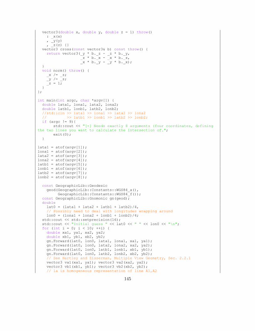
145
vector3(double x, double y, double z = 1) throw()
: _x(x)
, _y(y)
, _z(z) {}
vector3 cross(const vector3& b) const throw() {
return vector3(_y * b._z - _z * b._y,
_z * b._x - _x * b._z,
_x * b._y - _y * b._x);
}
void norm() throw() {
_x /= _z;
_y /= _z;
_z = 1;
}
};
int main(int argc, char *argv[]) {
double lata1, lona1, lata2, lona2;
double latb1, lonb1, latb2, lonb2;
//std::cin >> lata1 >> lona1 >> lata2 >> lona2
// >> latb1 >> lonb1 >> latb2 >> lonb2;
if (argc != 9){
std::cout << "[-] Needs exactly 8 arguments (four coordinates, defining
the two lines you want to calculate the intersection of.";
exit(0);
}
lata1 = atof(argv[1]);
lona1 = atof(argv[2]);
lata2 = atof(argv[3]);
lona2 = atof(argv[4]);
latb1 = atof(argv[5]);
lonb1 = atof(argv[6]);
latb2 = atof(argv[7]);
lonb2 = atof(argv[8]);
const GeographicLib::Geodesic
geod(GeographicLib::Constants::WGS84_a(),
GeographicLib::Constants::WGS84_f());
const GeographicLib::Gnomonic gn(geod);
double
lat0 = (lata1 + lata2 + latb1 + latb2)/4,
// Possibly need to deal with longitudes wrapping around
lon0 = (lona1 + lona2 + lonb1 + lonb2)/4;
std::cout << std::setprecision(16);
std::cout << "Initial guess " << lat0 << " " << lon0 << "\n";
for (int i = 0; i < 10; ++i) {
double xa1, ya1, xa2, ya2;
double xb1, yb1, xb2, yb2;
gn.Forward(lat0, lon0, lata1, lona1, xa1, ya1);
gn.Forward(lat0, lon0, lata2, lona2, xa2, ya2);
gn.Forward(lat0, lon0, latb1, lonb1, xb1, yb1);
gn.Forward(lat0, lon0, latb2, lonb2, xb2, yb2);
// See Hartley and Zisserman, Multiple View Geometry, Sec. 2.2.1
vector3 va1(xa1, ya1); vector3 va2(xa2, ya2);
vector3 vb1(xb1, yb1); vector3 vb2(xb2, yb2);
// la is homogeneous representation of line A1,A2

146
// lb is homogeneous representation of line B1,B2
vector3 la = va1.cross(va2);
vector3 lb = vb1.cross(vb2);
// p0 is homogeneous representation of intersection of la and lb
vector3 p0 = la.cross(lb);
p0.norm();
double lat1, lon1;
gn.Reverse(lat0, lon0, p0._x, p0._y, lat1, lon1);
// std::cout << "Increment " << lat1-lat0 << " " << lon1-lon0 << "\n"; //
I removed the output to save time. -CB
lat0 = lat1;
lon0 = lon1;
}
std::cout << "Final result " << lat0 << " " << lon0 << "\n";
double azi1, azi2;
geod.Inverse(lata1, lona1, lat0, lon0, azi1, azi2);
std::cout << "Azimuths on line A " << azi2 << " ";
geod.Inverse(lat0, lon0, lata2, lona2, azi1, azi2);
std::cout << azi1 << "\n";
geod.Inverse(latb1, lonb1, lat0, lon0, azi1, azi2);
std::cout << "Azimuths on line B " << azi2 << " ";
geod.Inverse(lat0, lon0, latb2, lonb2, azi1, azi2);
std::cout << azi1 << "\n";
}

147
7. Bibliography
[1] M. Longhi and G. Marrocco, “Ubiquitous Flying Sensor Antennas: Radiofrequency
Identification Meets Micro Drones,” IEEE Journal of Radio Frequency
Identification, vol. 1, no. 4, pp. 1–1, 2018.
[2] J. Flynt, “The Complete Drone Comparison,” 2018. [Online]. Available:
https://3dinsider.com/drone-comparison/. [Accessed: 28-May-2018].
[3] J. Robertson, “Why Bioshock still has, and will always have, something to say,”
2016. [Online]. Available: https://arstechnica.com/gaming/2016/08/bioshock-
objectivism-philosophy-analysis/. [Accessed: 28-May-2018].
[4] J. E. Hyten, “Brown Bag Lunch with USSTRATCOM Commander,” Wright-
Patterson AFB, 2016.
[5] FAA, “Sec. 336. Special Rule for Model Aircraft,” vol. 62, no. 9, pp. 62–68, 2012.
[6] forschungsbuero, “World’s first manned flight with an electric multicopter,” 2011.
[Online]. Available: https://www.youtube.com/watch?v=L75ESD9PBOw.
[Accessed: 28-May-2018].
[7] S. Kim, “Multirotor Configurations of an Unmanned Mini Aircraft,” IEEE 15th
International Conference on Networking, Sensing and Control, Zhuhai, China, 2018,
pp. 1–6.
[8] US Government Accountability Office, “Agencies Could Improve Information
Sharing and End-Use Monitoring on Unmanned Aerial Vehicle Exports,” 2012.
Available: https://www.gao.gov/products/GAO-12-536. [Accessed: 5-Jan-2019]
[9] R. T. Martorana, “WASP--A High-g Survival UAV,” in AIAA’s 1st Technical
Conference and Workshop on Unmanned Aerospace Vehicles, Portsmouth,
Virginia, 2002, pp. 34-39.
[10] DoD, “FY 16-27 PA. Lethal Minitaure Aerial Missile System (LMAMS)
Reprogramming Action,” 2016. [Online]. Available: https://admin.govexec.com
/media/16-27_pa_lmams_request.pdf. [Accessed: 28-May-2018]

148
[11] P. Tucker, “In Urgent Request , US Special Ops Adds 350 Kamikaze Drones to
Fight ISIS,” Defense One, 2017. [Online]. Available: https://www.defenseone.com/
technology/2017/05/Special-Ops-Gets-350-More-Kamikaze-Suicide-Drones-to-
Fight-ISIS/137987/. [Accessed: 28-May-2018].
[12] J. Gerts, “28th Annual Special Operations/Low-Intensity Conflict Symposium &
Exhibition,” 2017. [Online]. Available: http://www.ndia.org/-/media/sites/ndia/
meetings-and-events/3142-williams/meetings/2017/7880/final-agenda---web.ashx.
[Accessed: 27-May-2018]
[13] Gartner, “Gartner Says Almost 3 Million Personal and Commercial Drones Will Be
Shipped in 2017,” 2016. [Online]. Available: https://www.gartner.com/en/
newsroom/press-releases/2017-02-09-gartner-says-almost-3-million-personal-and-
commercial-drones-will-be-shipped-in-2017. [Accessed: 28-May-2018]
[14] The Economist, “Taking flight | Civilian Drones,” The Economist, 2017. [Online].
Available: https://www.economist.com/technology-quarterly/2017-06-08/civilian-
drones. [Accessed: 28-May-2018]
[15] D. Floreano and R. J. Wood, “Science, technology and the future of small
autonomous drones,” Nature, vol. 521, no. 7553, pp. 460–466, 2015.
[16] B. Canis, “Unmanned Aircraft Systems (UAS): Commercial Outlook for a New
Industry,” Congressional Research Service, pp. 1-17, 2015.
[17] D. Bamburry, “Drones: Designed for Product Delivery,” Design Management
Review, vol. 26, no. 1, pp. 40–48, 2015.
[18] E. Nowak, K. Gupta, and H. Najjaran, “Development of a Plug-and-play Infrared
Landing System for Multirotor Unmanned Aerial Vehicles,” 14th Conference on
Computer and Robot Vision, Edmonton, Alberta, Canada, 2017, pp. 256–260.
[19] D. Brescianini and R. D’Andrea, “Computationally Efficient Trajectory Generation
for Fully Actuated Multirotor Vehicles,” IEEE Transactions on Robotics, vol. 34,
no. 3, pp. 555–571, 2018.
[20] W. G. Aguilar, C. Angulo, and J. A. Pardo, “Motion intention optimization for
multirotor robust video stabilization,” in CHILEAN Conference on Electrical,
Electronics Engineering, Information and Communication Technologies,

149
CHILECON 2017 - Proceedings, Pucon, Chile, 2017, vol. 2017–January, pp. 1–4.
[21] H. M. C. W. B. Herath, H. M. S. Herath, S. W. Sumangala, O. De Silva, D.
Chathuranga, and T. D. Lalitharatne, “Design and development of an automated
battery swapping and charging station for Multirotor Aerial Vehicles,” in
International Conference on Control, Automation and Systems, Jeju, South Korea,
2017, vol. 2017–October, pp. 356–361.
[22] D. P. Koch, T. W. McLain, and K. M. Brink, “Multi-sensor robust relative
estimation framework for GPS-denied multirotor aircraft,” in 2016 International
Conference on Unmanned Aircraft Systems, Arlington, Virginia, 2016, pp. 589–597.
[23] C. F. Liew, D. DeLatte, N. Takeishi, and T. Yairi, “Recent Developments in Aerial
Robotics: A Survey and Prototypes Overview,” pp. 1–14, 2017.
[24] IEEE Computer Society Sponsored, “Part 11: Wireless LAN Medium Access Control
(MAC) and Physical Layer (PHY) Specifications IEEE Computer Society,” IEEE
Std 802.11, 2007.
[25] J. F. Kurose and K. W. Ross, Computer Networking: A Top-Down Approach, 6th
ed. Pearson, 2013.
[26] E. Skoudis and T. Liston, Counter Hack Reloaded: A Step-by-Step Guide to
Computer Attacks and Effective Defenses, 2nd ed. Pentice Hall, 2005.
[27] S. Fluhrer, I. Mantin, and A. Shamir, “Weaknesses in the Key Scheduling Algorithm
of RC4,” pp. 1–24, 2001.
[28] “Statistics.” [Online]. Available: https://wigle.net/stats#. [Accessed: 05-Jun-2018].
[29] Mahmoud Khasawneh, I. Kajman, R. Alkhudaidy, and A. Althubyani, “A Survey
on Wi-Fi Protocols: WPA and WPA2,” in Recent Trends in Computer Networks
and Distributed Systems Security, pp. 496–511, 2014.
[30] “Church of Wifi WPA-PSK Lookup Tables.” [Online]. Available:
https://www.renderlab.net/projects/WPA-tables/. [Accessed: 02-Jun-2018].
[31] L. Farhan, S. T. Shukur, A. E. Alissa, M. Alrweg, U. Raza, and R. Kharel, “A
survey on the challenges and opportunities of the Internet of Things (IoT),” in

150
Proceedings of the International Conference on Sensing Technology, Sydney,
Austrailia, 2018, vol. 2017–Decemember, pp. 1–5.
[32] A. J. Rose, “Security Evaluation and Exploitation of Bluetooth Low Energy
Devices,” AFIT Thesis AFIT-ENG-MS-17-M-066, 2017. Available: https://
www.dtic.mil/DTICOnline/downloadPdf.search?collectionId=tr&docId=AD10547
47. [Accessed: 04-Feb-2019]
[33] United States Defense Force, “Joint Publication 3-12 Cyberspace Operations,”
United States Defense Force, vol. 12, p. 62, 2013.
[34] J. Pearson, “An Ad Company Is Flying Surveillance Drones Over Los Angeles,”
Motherboard, 2015. [Online]. Available: https://motherboard.vice.com/en_us/
article/qkvmw3/an-ad-company-is-flying-surveillance-drones-over-los-angeles.
[Accessed: 04-Jun-2018].
[35] Y. A. De Montjoye, C. A. Hidalgo, M. Verleysen, and V. D. Blondel, “Unique in
the Crowd: The privacy bounds of human mobility,” Scientific Reports, vol. 3, pp.
1–5, 2013.
[36] J. Valente and A. A. Cardenas, “Understanding Security Threats in Consumer
Drones Through the Lens of the Discovery Quadcopter Family,” in Proceedings of
the 2017 Workshop on Internet of Things Security and Privacy, Dallas, Texas, 2017,
pp. 31–36.
[37] C. Dillow, “A DIY UAV That Hacks Wi-Fi Networks, Cracks Passwords, and Poses
as a Cell Phone Tower,” Poplular Science, 2011. [Online]. Available:
https://www.popsci.com/technology/article/2011-07/diy-uav-hacks-wi-fi-
networks-cracks-passwords-and-poses-cell-phone-tower. [Accessed: 01-Jun-2018].
[38] J. Greenwood, “The Phantom Menace - Weaponising a Consumer Drone,” 4Armed,
2015. [Online]. Available: https://www.4armed.com/blog/phantom-menace-
weaponising-drones/. [Accessed: 05-Apr-2018].
[39] Sensepost, “Snoopy: A distributed tracking and profiling framework,” Sensepost
Blog, 2012. [Online]. Available: https://www.sensepost.com/blog/7557.html.
[Accessed: 15-Jan-2019].
[40] F. Brown and D. Latimer, “Game of Drones: Putting the Emerging ‘Drone Defense’

151
Market to the Test,” in DEF CON 25, Las Vegas, Nevada, 2017. Available:
http://www.bishopfox.com/files/slides/2017/DEF_CON_25_(2017)-
Game_of_Drones-Brown_Latimer-29July2017.pdf. [Accessed: 04-Feb-2019]
[41] B. E. Law, “Passive Radiolocation of IEEE 802.11 Emitters Using Directional
Antennae,” AFIT Thesis AFIT-ENG-MS-18-M-040, 2018. Available: https://
www.dtic.mil/DTICOnline/downloadPdf.search?collectionId=tr&docId=AD10561
60
[42] S. M. Beyer, “Pattern-of-Life Modeling Using Data Leakage in Smart Homes,” AFIT
Thesis AFIT-ENG-MS-18-M-009, 2018. Available: https://www.dtic.mil/
DTICOnline/downloadPdf.search?collectionId=tr&docId=AD1055975. [Accessed:
04-Feb-2019]
[43] R. Aitken, “How much weight can delivery drones carry?” 2015 [Online]. Available:
http://unmannedcargo.org/how-much-weight-can-delivery-drones-carry/.
[Accessed: 07-Jan-2019].
[44] V. Dronelli, “7 drones that can lift heavy weights [2017 Edition],” DronesGlobe,
2017. [Online]. Available: http://www.dronesglobe.com/guide/heavy-lift-drones/.
[Accessed: 07-Jan-2019].
[45] D. D. N. Ltd., “NextG USB-Yagi TurboTenna Plug n Play Wi-Fi Antenna,” 2018.
[Online]. Available: http://www.danets.com/turbotenna/UsbYagi.php. [Accessed:
07-Jan-2019].
[46] A. Susset, “Beginner’s guide to IoT Cellular connectivity on Raspberry Pi and Linux
devices,” 2017. [Online]. Available: https://blog.soracom.io/beginners-guide-to-iot-
cellular-connectivity-on-raspberry-pi-and-linux-devices-55d4f7489adf. [Accessed:
07-Jan-2019].
[47] Plotly, Dash. Montreal, Quebec, 2018. Available: https://plot.ly/products/dash/.
[Accessed: 02-Feb-2019]
[48] Mapbox, Mapbox Maps. San Fransisco, CA, 2018. Available: https://
www.mapbox.com/maps/. [Accessed: 02-Feb-2019]
[49] C. F. F. Karney, “Geodesics on an ellipsoid of revolution,” 2011. [Online]. Available:
https://arxiv.org/pdf/1102.1215.pdf. [Accessed: 5-Jan-2019]

152
[50] W. J. H. T. Center, “Global Positioning System (GPS) Standard Positioning Service
(SPS) Performance Analysis Report,” pp. 1–61, 2014.
[51] Fred Klassen, Tcpreplay. Boston, MA, 2018. Available: https://github.com/
appneta/tcpreplay. [Accessed: 11-Feb-2019]

153
172