customer segmentation, allocation planning and order promising in make-to-stock production

OR Spectrum (2009) 31:229–256DOI 10.1007/s00291-008-0123-x

REGULAR ARTICLE

Customer segmentation, allocation planning and orderpromising in make-to-stock production

Herbert Meyr

Published online: 13 February 2008© Springer-Verlag 2008

Abstract Modern advanced planning systems offer the technical prerequisites foran allocation of “available-to-promise” (ATP) quantities—i.e. not yet reserved stockand planned production quantities—to different customer segments and for a realtime promising of incoming customer orders (ATP consumption) respecting allocatedquota. The basic idea of ATP allocation is to increase revenues by means of customersegmentation, as it has successfully been practiced in the airline industry. However,as far as manufacturing industries and make-to-stock production are concerned, it isunclear, whether, when, why and how much benefits actually arise. Using practical dataof the lighting industry as an example, this paper reveals such potential benefits. Fur-thermore, it shows how the current practice of rule-based allocation and consumptioncan be improved by means of up-to-date demand information and changed customersegmentation. Deterministic linear programming models for ATP allocation and ATPconsumption are proposed. Their application is tested in simulation runs using thelighting data. The results are compared with conventional real time order promisingwith(out) customer segmentation and with batch assignment of customer orders. Thisresearch shows that—also in make-to-stock manufacturing industries—customer seg-mentation can indeed improve profits substantially if customer heterogeneity is highenough and reliable information about ATP supply and customer demand is available.Surprisingly, the choice of an appropriate number of priority classes appears moreimportant than the selection of the ATP consumption policy or the clustering methodto be applied.

H. Meyr (B)Chair of Production and Supply Chain Management,Technical University of Darmstadt,Hochschulstr. 1, 64289 Darmstadt, Germanye-mail: [email protected]

123

230 H. Meyr

Keywords Available-to-Promise (ATP) · Advanced planning systems · Clustering ·Integer and linear programming · Order promising

1 Introduction

One of the biggest challenges in airline industry is to avoid that a hasty, high marginbusiness class customer cannot get a seat because a low price economy customerhas booked the last one a few minutes ago. Revenue management has developedtechniques to treat such problems adequately, e.g. to establish and fence off customersegments in form of booking classes and to determine booking limits. The situation isdifferent in make-to-stock (MTS) supply chains of consumer goods industries wherefinal item stocks are built up on basis of forecasts and customer requests are served fromthis stock. But not too different. Here, too, exist more important and less importantcustomers yielding higher and lower profit margins. Here, too, occur shortages. Anda service level of 98 percent also implies that two percent of the customers have notbeen served as desired. This may concern several dozens of orders per day, for a singleitem only. “Not as desired” not necessarily means that the customers are not suppliedat all. However, late deliveries lead to customer annoyance and customer migration inthe long term. Thus here, too, it is important to consider carefully who gets its goodson time and—even more crucially—who does not.

Actually “order promising”, i.e. communicating the customer a reliable andhopefully soon delivery date, is the planning task to be considered. However, inMTS situations order promising also means deciding about— and for short-termorders simultaneously releasing—delivery (see Fleischmann and Meyr 2003a). Thus,these decisions about actual deployment can hardly be re-thought. In order to promisereliable delivery dates, modern enterprise resources planning (ERP) systems or advan-ced planning systems (APS) build on up-to-date information about stock on hand andplanned supply of the distribution centers that both not yet have been assigned tocustomers. Such unreserved quantities are called “available-to-promise”(ATP). Sinceproduction has to be planned on basis of forecasts (push concept implied by MTS),unused production capacity, sometimes called “capable–to–promise”, and stock re–filling are no more concern at this point in time. The information about the plannedsupply of the distribution centers either stems from the short–term master productionschedule of a single, corresponding production plant or—for a longer preview—evenfrom a mid–term production and delivery plan (“master plan”) of the overall supplychain (see e.g. Kilger and Meyr 2008).

Usually two different modes of promising ATP to incoming customer orders aredistinguished, “batch order processing” and real time “single order processing” (seee.g. Ball et al. 2004; Fleischmann and Meyr 2003a; Pibernik 2005). In batch mode,an order is not promised immediately upon request, but held back. It is then assignedto ATP inventories together with several other orders in a “batch”. Thus, there mustbe enough time to gather these orders and a customer must be willing to wait for ananswer. Often, this “batching horizon” comprises several hours or a whole day.

Sometimes customers expect an immediate answer for their order query. In thiscase batching of orders is not possible. Thus, each single order has to be processed inreal time and ATP is consumed in a first-come-first-served (FCFS) manner.

123

Customer segmentation, allocation planning 231

As addressed in the airline example above, in shortage situations, where demandis higher than capacities—i.e. in this case than ATP inventories—single order proces-sing entails the danger of promising scarce inventory to the wrong customers, e.g. toless important customers or to customers showing smaller profit margins. Allocationplanning, as propagated by APS vendors like i2 and SAP (see Kilger and Meyr 2008),promises to be a way to improve real time single order processing by reserving sharesof the ATP, the so-called “quotas” or “allocated ATP”, for important customers in themedium term and afterward promising orders with respect to these allocated quotasin the short term. That means ATP is held back in anticipation of later arriving, moreprofitable orders even if a less profitable order already requests this stock. Such anallocation of quotas shall take advantage of a customer segmentation into low andhigh priority customers as it has shown to be successful in airline industries. Thisleads to a two step ATP allocation and ATP consumption process, in the followingcalled “allocation planning and ATP consumption” (AP&C).

It is important to note that such a segmentation already appears useful if the sameproduct is sold for different profits or with different priorities. For example, varioussales channels might generate different profit margins because sales prices vary due tocountry-specific tax levels or due to differing transport costs. Or in-house customersmight show other strategic importance for a company than external customers. All inall, the AP&C approach promises to be useful for companies which produce storablestandard products in high volume on an MTS basis and whose multitude of customersare heterogeneous in the above sense. Then, there is the hope that the same or evenbetter profits as in batch mode can be achieved, even though a customer gets his answerimmediately.

The intention of this paper is to structure the AP&C process and to reveal thepotential benefits of allocation planning as compared to the common practices of FCFSsingle order processing or batch order processing. However, before the contributionof the paper can be specified in some more detail, a brief review of current practicesand existing literature is necessary.

1.1 Literature review

For a literature review we will concentrate on ATP support for commercial (ERP and)advanced planning systems and especially discuss papers which tackle ATP allocationor consumption in more detail. Note that we focus on MTS situations, i.e. the ATPsupply of finished items is assumed to be fixed because it bases on the stock on handand on the production quantities that have already been planned in the short-termproduction scheduling module of the APS and/or a mid–term master planning module(see e.g. Meyr et al. 2008). This rules out literature on make–to–order (MTO) andassemble–to–order (ATO) supply chains, which most of the due date setting (see e.g.Keskinocak and Tayur 2004) and batch order promising models (see e.g. Chen et al.2001, 2002) have been developed for. In these situations customers are usually willingto wait longer for an order promise than in MTS supply chains. This also rules outinventory rationing (see e.g. de Vericourt et al. 2002), which explicitly allocates stockson hand to several customer classes, but assumes that the refilling of the stock can stillbe influenced by means of orders. Finally, it also excludes revenue management (see

123

232 H. Meyr

e.g. Talluri and Van Ryzin 2004), where “capacities” are assumed to be perishableand thus stocks cannot be held at all. A deeper discussion of the relationship betweenthese various, but similar types of models and their applications in industry wouldgo beyond the scope of this paper. Instead, the reader who is interested is referred toQuante et al. (2008).

Demand fulfillment and order promising on the basis of ATP information is oneof the most popular planning tasks (see Kilger and Wetterauer 2008, Table 16.1)covered by commercial APS. A general overview regarding APS and the role of ATPtherein is given by Fleischmann and Meyr (2003b) and Stadtler and Kilger (2008).Fleischmann and Meyr (2003a) classify different situations of demand fulfillment withrespect to the three order penetration points MTO, ATO and MTS. They also pointout that—as opposite to MTO and ATO — in MTS situations it often is sufficientto consider each product separately. Pibernik (2005) also characterizes different ATPapplications and models. He implicitly uses a similar categorization by distinguishingthe operating mode (real time/batch), the availability level of goods and the interactionwith manufacturing planning, where the two latter ones are usually used to characterizethe different order penetration points. ATP software modules of several APS vendorsare presented by Meyr et al. (2008). Dickersbach (2004, Sect. 11) and Knolmayeret al. (2002, Sect. 3.1.5), however, put a special emphasis on the Global ATP moduleof SAP’s advanced planner and optimizer (APO).

The paper of Kilger and Meyr (2008) is basic for the following sections because itpresents the implementation of demand fulfillment in APS in a sufficiently high detail.Kilger and Meyr (2008) especially describe the simple rules that are usually appliedin APS for both allocation planning (Sect. 9.4) and ATP consumption (Sect. 9.5).Whereas their argumentation mainly bases on experiences with software of the APSvendor i2, Dickersbach (2004, Sects. 11.2 and 11.3) shows that a similar approachhas also been favored by SAP/APO. Allocation planning rules, for example, quotean overall ATP quantity to different customer classes on basis of priority rankings,with respect to some pre-defined fixed shares or proportional to the original forecastsof different customers or markets. ATP consumption rules, for instance, allow accessto allocated ATP of an order’s corresponding class or to ATP of classes showinglower priority. If customers have not been segmented—and thus the above allocationplanning is useless—ATP that has been assigned to other time buckets, to substituteproducts or to other locations (e.g. distribution centers or regional warehouses) issearched for in an user–defined sequence.

Fischer (2001) compares such ATP consumption rules for single order processingwith a linear programming (LP) based batch order processing for a practical caseof the lighting industry and shows advantages of the batch mode. It is interesting tonote that this lighting company originally distinguished eight classes of customersshowing different importance, which have—for sake of simplicity — been reduced tothree by Fischer. In a similar MTS environment Pibernik (2006) compares differentATP consumption rules for managing the stock outs of a pharmaceutical company.He suggests to change from a single order to a batch order processing mode only ifshortage is foreseeable. Even though this company also segments their customers intofive priority groups, allocation planning is tested only rudimentarily by Pibernik, usinga “naive” allocation scheme reserving stock for the two most important groups only.

123


As mentioned above, the APS allocation rules either make no assumptions aboutdemand (for example priority rankings) or use short–term demand forecasts in a ratherdoubtful manner, e.g. by allocating production quantities and ATP proportionally tothe demand forecasts, which has been shown to increase the bullwhip effect withinsupply chains (see Lee et al. 1997). Instead, Ball et al. (2004, Chap. 15.4.2) propose anLP based deterministic allocation model. Basically, it summarizes linear and mixedinteger programming models of hierarchical production planning that are used toallocate aggregate inventory of product families and/or limited production capacity tovarious items within a family. Obviously, this general idea can be transferred to allocateATP to different customer classes. Although the model proposed by Ball et al. oughtto be applied in an MTS environment, it rather fits ATO supply chains because it alsodecides about raw material and capacity usage. A more convenient MTS applicationof this type of models is presented below in Sect. 2.3.

Summing up, modern APS offer the technical prerequisites for ATP allocation andATP consumption, thus hoping to gain similar advantages in manufacturing industriesas have been achieved by revenue management principles in airline or hotel indus-tries. However, they only provide very simple allocation and consumption rules, andfurthermore do not give advices how and when to apply them. Thus, overall benefitsare doubtful. Looking through scientific literature is hardly helpful in this specificsituation because either the model assumptions do not fit (e.g. stochastic inventoryrationing) or the overall performance of both allocation and consumption policieshas not been tested for potential alternatives of customer segmentation (for example,(Fischer 2001; Pibernik 2005) take the segmentation for granted).

1.2 Contribution and organization of the paper

The basic idea of this paper is to improve demand fulfillment in MTS supply chainsby making use of the heterogeneity of different customers through AP&C order pro-mising. The fundamental steps are:

• To segment customers with respect to their importance and profitability into severalpriority classes,

• to allocate ATP to these classes on basis of a deterministic profit maximizationprocess taking advantage of short–term demand information, and

• to promise customer orders, i.e. to consume ATP, in real time with respect to thesecustomer hierarchies.

In order to demonstrate the usefulness, all steps will be executed in a holistic simulationexperiment exploiting practical data of the lighting industry. To our knowledge, sucha comprehensive test, including customer segmentation and allocation, is missing sofar. The aim is to structure the planning tasks concerned with AP&C and to gainideas whether and how a preceding allocation process—making use of the short–terminformation provided by APS—may be advantageous compared to the traditionalfirst-come-first-served single order processing.

The next section introduces appropriate LP models for demand fulfillment in MTSsupply chains. Numerical experiments with data of the lighting industry are run in

123

234 H. Meyr

Sect. 3. A summary of the methodology proposed and of the managerial insightsgained concludes the paper.

2 Model formulations

The following section describes the modeling environment that allows to compare thedifferent ways of order promising and ATP assignment. LP models for single and batchorder processing without customer segmentation are proposed in Sect. 2.2, whereasSect. 2.3 introduces the allocation planning model making use of segmentation. Allmodels aim at profit maximization. Their outcome can be compared directly withthe optimal profit that would result from a simultaneous ex–post assignment of allorders arriving within the planning horizon, which is called “global optimization” inthe following.

2.1 Modeling environment

The different order promising alternatives verbally described in the introduction willnow be represented by mathematical models. Figure 1 shows the modeling environment

a-c without customer segmentation:

supply planning(e.g. production

planning)

ATP consumption(“order promising”)

“customer”

ATP

order(s) commit-ment(s)

a) GO: once for all orders of the planning horizon T

b) BOP: several times for all ordersof a batching horizon B<<T

c) SOP: in real-time for each single order

supply planning

ATP allocation(“allocation planning”, AP)

“customer”

ATP

singleorder

singlecommitment

demand planning

forecasts

ATP consumption (SOPA)

allocated ATP(= quotas

for customerclasses k)

d) with customer segmentation:

once

once

real-time

real-time

once forplanninghorizon T

real-time

a-c

Fig. 1 Modeling environment for the models “Global Optimization” (GO), “Batch Order Processing”(BOP) and “Single Order Processing” (SOP) without customer segmentation and “Allocation Planning”(AP) and “SOP after allocation planning” (SOPA) with customer segmentation

123


that was chosen to do this. The models (a–c) that do not distinguish customer segmentsshall be compared with the AP&C models (d) which put the revenue management ideaof the introductory example into practice by differentiating different customer classesk, allocating ATP to these customer classes and satisfying customer demand only ifenough allocated ATP of the customer’s corresponding class is available.

For this, the finite, overall planning horizon T is subdivided into discrete timebuckets t = 1, . . . , T . Once, at the beginning of planning (t = 0), on the basis ofsupply information—e.g. from the master production schedule or master plan—it iscalculated how much ATP becomes available in each period t (for this calculation seee.g. Fleischmann and Meyr 2003a,b). Customer orders i arrive one after each otherat different arrival dates ai . For each order i it is known, how much the customerwants to get (“requested delivery quantity” qi ) and when he wants to get this quantity(“requested delivery date” di , i.e. the time bucket t , for which the customer requestshis order i to be delivered). The limited availability of ATP necessitates that not allorders can be served on time. The “order promising” or “ATP consumption” problemis to decide whether, when and to which degree each order will be served from theATP. Not fulfilling an order on time or not filling an order at all will be punished bypenalty costs diminishing the original profit the order would leave. ATP is assumed tobe known deterministically at t = 0, for the whole planning horizon T . Thus it needsonly to be updated when orders are accepted but not because its supply has changedunexpectedly.

The models (a–c) without customer segmentation differ according to the number oforders that are gathered before the orders are processed, i.e. assigned to the differentperiods’ ATP by means of an LP model maximizing the profit of all incoming orders.The “Single Order Processing” model SOP processes each order immediately in realtime and thus is trivial to be solved. The “Batch Order Processing” model BOP gathersall orders arriving within a batching horizon B � T . The “Global optimization” modelGO gathers all orders of the whole planning horizon T . Of course, since T is a quitelong time span (e.g. a month) it is not realistic that customers will wait so long untilgetting a promise. However, because all orders of the whole planning horizon arecovered and optimized simultaneously, this model can serve as a benchmark to judgethe performance of an iterative application of the other models.

Situation (d) is modeled by a sequence of an “Allocation Planning” model AP thatis executed once at t = 0 and several single order processing models—now denoted as“Single Order Processing After allocation planning” (SOPA)—which are executed inreal time when each new customer order arrives. The AP model once allocates ATP tothe different, a priori known customer classes k by means of linear programming. Forthis, up-to-date forecasts of customer demand within each customer class are necessary.Like in (c) each single order is processed in real time, but it is only allocated to thedesired delivery date if enough allocated ATP (aATP) of its respective customer classis available and can be consumed. This corresponds to the revenue management andinventory rationing idea that some portion of scarce stock should be held back formore important orders which might arrive later on.

The motivation for this kind of deterministic, mathematical modeling originatesfrom current practice of APS usage (see e.g. Kilger and Meyr 2008). ATP and demandforecasts are calculated in APS anyway and can be aggregated for different customer

123

236 H. Meyr

classes. Also basic allocation and consumption rules are used. Thus, the fundamen-tal technical framework for its application already exists. Furthermore, LP as a moresophisticated allocation method could probably easily be implemented because it isused for mid–term master planning and strategic network design, anyway (Fleisch-mann and Meyr 2003b).

Of course, very simplifying assumptions are made in this modeling environment ascompared to practice. For example partial delivery of orders is assumed to be possible,no bargaining about delivery dates is allowed, customer service can only be expressedin terms of money and uncertainties of demand and supply are excluded. The latterproblem, for instance, could be tackled by introducing a rolling horizon planning onat least two planning levels: a mid-term (e.g. weekly rolling) level for updating supplyinformation and executing allocation planning and a short-term (e.g. daily rolling forBOP or real-time for SOP/SOPA) level for ATP consumption. In this case ATP updateswould be necessary weekly after each update of supply information, but also dailyor for each order (see e.g. Fleischmann and Meyr 2003a, for ATP re-calculation).AP runs would also be necessary weekly, after each supply and subsequent ATPupdate, and would base on the latest forecasts on customer demand. However, a moredetailed discussion of these application issues would go beyond the scope of thispaper because, first, structural insights on the negative impacts of the decompositionof the GO problem into subsequent BOP, SOP or AP/SOPA models should be gained.Thus, the restrictive assumptions are necessary to exclude side effects, e.g. due to badforecasting of supply and demand. Of course, in a next step, these assumptions shouldbe weakened (see Sect. 4).

In the following, the situation (a–c) without customer segmentation is described inmore detail by introducing a single, “basic” order promising model that is applied indifferent ways to gain the models GO, BOP and SOP.

2.2 Models without customer segmentation

The basic order promising model is a simple network flow problem where the requestedquantities qi —in the following also called “demand”—of certain customer ordersi = 1, . . . , I have to be satisfied by ATP inventories AT Pt that become availablein discrete periods t = 1, . . . , T , e.g. days or weeks. In order to ensure feasibilityeven if demand is higher than ATP inventory, a fictitious period T + 1 has beenintroduced being able to serve the surplus demand by setting AT PT +1 := ∑I

i=1 qi −∑T

t=1 AT Pt . The goal is to find the part oit of order i that has to be satisfied byATP of period t so that the overall profit is maximized for a given per unit profitpit . This per unit profit can, for example, be computed by subtracting the per unitcosts ci from the per unit revenues ei of the order i and by punishing the use of ATPfrom periods earlier (necessitating storage) or later (backlogging) than the customer’srequested delivery date di . ATP of the fictitious period T +1 models non-delivery andthus cannot generate any profit (pi, T +1 = 0). It may even cause a loss of goodwillbeing punished by negative profits pi, T +1 < 0. Note that costs and revenues ofdifferent customers/orders may vary individually, e.g. due to different transportation

123


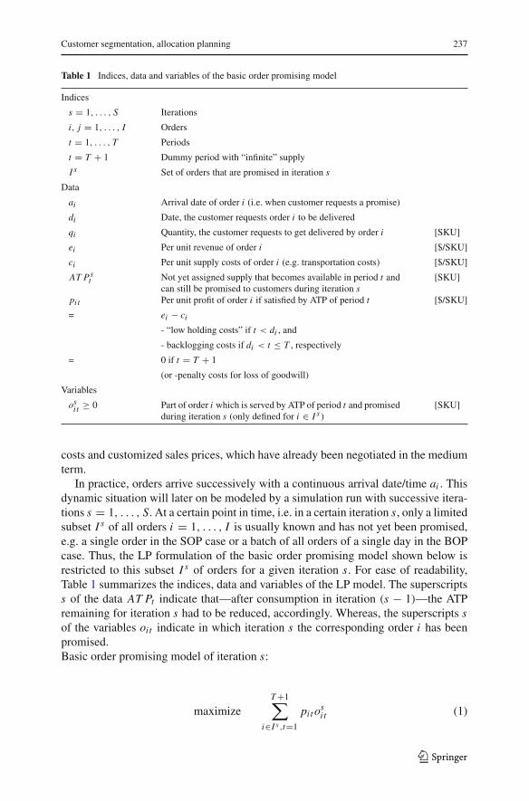
Table 1 Indices, data and variables of the basic order promising model

Indices

s = 1, . . . , S Iterations

i, j = 1, . . . , I Orders

t = 1, . . . , T Periods

t = T + 1 Dummy period with “infinite” supply

I s Set of orders that are promised in iteration s

Data

ai Arrival date of order i (i.e. when customer requests a promise)

di Date, the customer requests order i to be delivered

qi Quantity, the customer requests to get delivered by order i [SKU]

ei Per unit revenue of order i [$/SKU]

ci Per unit supply costs of order i (e.g. transportation costs) [$/SKU]

AT Pst Not yet assigned supply that becomes available in period t and

can still be promised to customers during iteration s[SKU]

pit Per unit profit of order i if satisfied by ATP of period t [$/SKU]

= ei − ci

- “low holding costs” if t < di , and

- backlogging costs if di < t ≤ T , respectively

= 0 if t = T + 1

(or -penalty costs for loss of goodwill)

Variables

osit ≥ 0 Part of order i which is served by ATP of period t and promised

during iteration s (only defined for i ∈ I s )[SKU]

costs and customized sales prices, which have already been negotiated in the mediumterm.

In practice, orders arrive successively with a continuous arrival date/time ai . Thisdynamic situation will later on be modeled by a simulation run with successive itera-tions s = 1, . . . , S. At a certain point in time, i.e. in a certain iteration s, only a limitedsubset I s of all orders i = 1, . . . , I is usually known and has not yet been promised,e.g. a single order in the SOP case or a batch of all orders of a single day in the BOPcase. Thus, the LP formulation of the basic order promising model shown below isrestricted to this subset I s of orders for a given iteration s. For ease of readability,Table 1 summarizes the indices, data and variables of the LP model. The superscriptss of the data AT Pt indicate that—after consumption in iteration (s − 1)—the ATPremaining for iteration s had to be reduced, accordingly. Whereas, the superscripts sof the variables oit indicate in which iteration s the corresponding order i has beenpromised.Basic order promising model of iteration s:

maximizeT +1∑

i∈I s ,t=1

pit osit (1)

123

238 H. Meyr

subject to

T +1∑

t=1

osit = qi ∀ i ∈ I s (2)

∑

i∈I s

osi t ≤ ATPs

t ∀ t = 1, . . . , T (3)

The overall profits of satisfying the orders i ∈ I s from ATP inventory are maximizedby the objective function (1). The requested quantity qi of each order i has to be metexactly, either by “real” supply of a regular period t = 1, . . . , T or by the “fictitioussupply” modeling non–delivery (2). Constraints (3) ensure that the supply capacitycannot be exceeded, i.e. that only the still available ATP of period t can be assignedto yet unpromised orders i ∈ I s .

This basic order promising model will be applied for simulating the three scenarios(a), (b) and (c) of Fig. 1. With i(s) := argmini {ai : i ∈ I s} denoting the order i ∈ I s

having the earliest arrival date during iteration s, the following three situations—justdiffering by the cardinality |I s | of the subsets I s—can be distinguished:

(a) GO: all orders of the planning horizon T are known in advance and are consideredin a single optimization run, i.e. I s := {1, . . . , I } and S := 1.

(b) BOP: only subsets of orders within a “batching horizon” of B periods are consi-

dered, i.e. I s :={

i :⌊

ai(s)

⌋≤ ai <

⌊ai(s)

⌋+ B

}and S := T/B with

⌊ai(s)

⌋

denoting the period t the arrival of order ai(s) is assigned to (assuming that T isan integer multiple of B).

(c) SOP: only a single order is considered during an iteration s, i.e. I s := {i(s)} andS := I . This is the case for real time due date assignment on an FCFS basis.

Since the degree of freedom decreases, it is expected that the overall objective functionvalues of these models decrease, too, i.e. GO� ≥ ∑T/B

s=1 BOP�s ≥ ∑I

s=1 SOP�s with

a � denoting the optimal solution of a model. As already mentioned, GO� can serveas a benchmark (“first best solution”), showing what profit would be optimal if therewere perfect knowledge of customer demand for the whole planning horizon T . Thevalues SOP� := ∑I

s=1 SOP�s and BOP� := ∑T/B

s=1 BOP�s are directly comparable to

GO�. They show the loss of profit that has to be accepted if, for the sake of customerservice, real time order promising or a short batching horizon B have to be realized.

To compute SOP� and BOP� in a simulation experiment, the remaining ATP has tobe updated according to ATPs+1

t := ATPst − ∑

i∈I s os�i t ∀t = 1, . . . , T in-between

the iterations s and s+1. This corresponds to the inventory netting and ATP calculationprocedure, more generally described by Fleischmann and Meyr (2003a), for the specialcase that supply is assumed to be deterministically known in advance. AT P1

t canbe initialized by inventory on hand (t = 0) and the projected supply (accordingto the master production schedule or master plan of the supply chain) of periodst = 1, . . . , T . Without loss of generality, AT Ps

0 = 0 ∀s is assumed in the following.

123


2.3 Models with customer segmentation

The above formulas give rise to the suspicion that BOP� can be brought closer to G O�

by simply increasing the batching horizon B. This behavior has already been confirmedby the experiments of Chen et al. (2002, 2001). However, customer expectations ofshort order promising response times set a natural limit to an increase of B. Thusmodern APS follow another approach to close the gap to G O� while simultaneouslyoffering the real time single order response times of SOP. As described by Kilgerand Meyr (2008), they adapt ideas of revenue management for industrial purposes:scarce capacity (in this case ATP) is allocated to certain customer classes with differentpriorities (or profits). Incoming customer orders are allowed to consume capacity oftheir own or a lower priority class only. By doing this, it shall be prevented that alower priority customer order can consume capacity that would later on be needed fora higher priority order gaining higher profits.

Thus, single order promising can still be applied, but it is preceded by an earlierallocation (sometimes called “quoting”) process, reserving ATP for distinct priorityclasses. It is the aim of this paper to model the planning problems arising in such acontext and to demonstrate and quantify the potential benefits of such a procedure.Therefore, the ATP allocation and ATP consumption processes of situation (d) in Fig. 1have been put into the same modeling and simulation environment as GO, BOP andSOP in a–c of Fig. 1 and the LP models AP and SOPA have been designed to representboth partial problems: The allocation planning model AP first assigns ATP to a pre-defined number K of customer (or more generally: priority) classes k = 1, . . . , K . Thesubsequent single order consumption SOPA of the class-specific ATP is also modeledand solved by LP, even if APS usually apply simpler and faster rule-based algorithmsfor the ATP consumption. Section 2.4 finally demonstrates how orders can be assignedto priority classes.

Table 2 shows the indices, data and variables of the AP model. As can be seen,agreements on how much has to be sold at a minimum (lower bound on sales quantity)to a respective priority class k in a certain period t and forecasts on how much can atmost be sold (upper bound on sales quantity) are needed in order to quote ATP withrespect to the expected profits of the respective classes. The lower bounds usuallyrepresent strategic sales targets or mid-term commitments which ensure that certaincustomer groups get a minimum level of service. The upper bounds are estimates ofthe aggregate customer demand of the respective class in a certain period, i.e. forecastson what all customers of this class will buy at a maximum. The degree to which thedemand of a certain class should (in terms of overall profits) actually be satisfied willbe determined by the model. Thus, with respect to the limited ATP capacity, the modelfurther restricts potential sales to certain customer classes by allocating ATP to themost profitable ones.

In detail, the AP problem can be formalized as follows:Allocation planning problem (AP):

maximizeT +1∑

k,t=1

T∑

τ=1

pktτ · zktτ (4)

123

240 H. Meyr

Table 2 Indices, data and variables of the allocation planning problem (AP)

Indices

k = 1, . . . , K Priority (or profit) classes of orders/customer groups

(The number of classes K has to be pre–defined in advance).

�k Set of orders i belonging to priority class k

Data

dminkt (≥ 0) Lower bound on sales to priority class k in period t [SKU]

dmaxkt (≥ dmin

kt ) Estimated (maximum) customer demand of class k in period t [SKU]

(= upper bound on sales quantity to priority class k in period t)

pktτ Per unit profit if ATP of period t (= 1, . . . , T + 1) satisfiesdemand of priority class k in period τ (= 1, . . . , T ), e.g.

[$/SKU]

= Per unit revenue ek in priority class k

-supply costs c

-“low holding costs” if t < τ , and

-backlogging costs if τ < t ≤ T , respectively

= 0 if t = T + 1

(or -penalty costs for loss of goodwill)

Variables

zktτ ≥ 0 Part of demand of priority class k in period τ (= 1, . . . , T )

which is satisfied by ATP in period t (= 1, . . . , T + 1)

[SKU]

ft ≥ 0 Still unallocated part of ATP in period t [SKU]

subject to

dminkτ ≤

T +1∑

t=1

zktτ ≤ dmaxkτ ∀ k, τ = 1, . . . , T (5)

T∑

k,τ=1

zktτ + ft = ATP1t ∀ t = 1, . . . , T (6)

ATP is allocated to the priority classes k so that the overall profit is maximized (4).The per unit profits pktτ of a class k can, for example, be computed as the averageprofits pit of the orders i ∈ �k that have been assigned to class k. The totally reservedATP has to be within the upper and lower sales bounds of the respective priorityclass (5). If, due to the upper bounds dmax

kτ , ATP cannot be assigned to one of theclasses, it remains unallocated (6) and thus can be used by any class in the later SOPAconsumption.

As already explained in Sect. 2.1, when facing supply and demand uncertainty, APshould be done on a rolling horizon basis. However, since supply uncertainty shouldnot matter in the simulation experiments of Sect. 3, AP only needs to be executedonce at the beginning of planning in t = 0. Further, to exclude forecast errors (demanduncertainty), the aggregate demand forecast dmax

kτ of class k is initialized with the (lateron) actually requested quantities, i.e. dmax

kτ := ∑i∈�k :di =τ qi ∀k, τ with �k denoting

123


Table 3 Indices, data and variables of the SOPA problem in iteration s

Indices

classi Priority class order i belongs to

�i Set of priority classes which can be consumed by order i

Data (ATP that can be consumed by order i(s) in iteration s)

aATPsktτ ATP that becomes available in period t and has been allocated to orders

in priority class k with a requested delivery date in period τ

[SKU]

uATPst ATP that becomes available in period t but has not yet been allocated to

any priority class or planned delivery date[SKU]

Variables

oskt ≥ 0 Part of allocated ATP of priority class k in period t (= 1, . . . , T + 1)

which is in iteration s assigned to order i(s) showing a requested deliverydate di(s)

[SKU]

xst ≥ 0 Part of unallocated ATP of period t , which is in iteration s assigned to

order i(s) showing a requested delivery date di(s)

[SKU]

the priority class which order i belongs to and di denoting the requested deliveryperiod of order i . For ease of simplicity, the lower bounds on sales are set to zero,i.e. dmin

kτ := 0 ∀k, τ .The optimal solution z�

ktτ of AP allows a very detailed allocation of ATP, not onlyspecifying the period t , the ATP becomes available, but also specifying which priorityclass k it should be reserved for and in which period τ it should be consumed. LetaATPs

ktτ denote allocated ATP that has been defined on the same level of granularityand remains available for consumption in iteration s. Then, the allocated ATP of thefirst period after the allocation procedure AP can be defined according to

aATP1ktτ := z�

ktτ ∀k, t, τ, (7)

thus allowing a very restrictive reservation for important classes. This appears usefulif the forecasts of customer demand are very reliable. Of course, if forecast accuracyis low, also a more aggregate allocation could be applied, e.g. by

aATP1kt :=

T∑

τ=1

z�ktτ ∀k, t. (8)

The quantities uATP1t := f �

t ∀t remain unallocated in case the expected ATP inven-tories are higher than estimated demand. If, on the other hand, estimated demand isexpected to be higher than total ATP inventories, the portion of demand of period t inclass k that has been allocated to z�

kt,T +1 > 0 by (5) cannot be served later on.The LP model (9)–(12) uses these allocated and unallocated ATP quantities as an

input for real time single order processing after allocation planning. The variables ofthis SOPA model are explained in Table 3. Since the SOPA models of the subsequentsimulation iterations consider a single order, each, the only order of iteration s isdenoted by i(s) in the following:

123

242 H. Meyr

“SOP after allocation planning” model of iteration s (SOPAs):

maximize∑

k∈�i(s)

T +1∑

t=1

pi(s),t oskt +

T∑

t=1

pi(s),t xst (9)

subject to

∑

k∈�i(s)

T +1∑

t=1

oskt +

T∑

t=1

xst = qi(s) (10)

oskt ≤ aATPs

ktdi(s)∀ k ∈ �i(s), t = 1, . . . , T (11)

xst ≤ uATPs

t ∀ t = 1, . . . , T (12)

In (9) the original profits pit of Table 1 are maximized. Thus, the simulation resultSOPA� := ∑S

s=1 SOPA�s of a preceding AP optimization, followed by S := I ite-

rations of SOPA (with an optimal objective function value SOPA�s of iteration s), is

directly comparable to GO�, BOP� and SOP� as computed in Sect. 2.2. The Eqs. (10)ensure that the requested quantity of order i(s) is either met by (un)allocated ATPor assigned to the fictitious period T + 1 and thus denied, however generating noprofit or even incurring penalty costs. The capacity constraints (11) and (12) limitthe use of allocated and unallocated ATP to their predefined values. An order i(s)can only consume ATP in some dedicated classes �i(s). For example, by setting

�i(s) := {k : classi(s) ≥ k ≥ K } it can be ensured that an order i(s) ∈ �l canonly consume ATP of its own priority class l := classi(s) or other classes k > l sho-wing lower priorities. Thus, also for the AP problem, it is assumed that the classesk = 1, . . . , K have been sorted according to decreasing priorities, e.g. defining k > lif the average profits fulfill

∑t, i∈�k

pit

|�k | ≤∑

t, i∈�lpi t

|�l | . (13)

Such a strategy of allowing access to lower priority ATP has, for example, been appliedby Fischer (2001)—there called “hierarchical cumulated quoting”—or by Kilger andMeyr (2008) using customer hierarchies.

Analogously to the SOP procedure described in Sect. 2.2, in the following simula-tion experiments the (un)allocated ATP remaining after iteration s for use in iterations + 1 can easily be calculated by (14) and (15):

a AT Ps+1ktdi(s)

:= a AT Psktdi(s)

− os�kt ∀ k, t = 1, . . . , T, (14)

u AT Ps+1t := u AT Ps

t − x�t ∀ t = 1, . . . , T . (15)

As already mentioned in Sect. 2.1, this is possible because demand and supply areassumed to be known in advance. Such a data update is more complicated if demand

123


and supply are uncertain and if AP is executed on a rolling horizon basis. In this caseinventory netting and ATP calculation as described by Fleischmann and Meyr (2003a)are necessary. Note that in MTS situations late delivery or cancellation of orders is onlypossible for newly arriving orders but not for orders that have already been promised(and thus delivered!). This is opposite to order promising in ATO or MTO situations.

Applying AP/SOPA instead of GO can be seen as a kind of problem decompositionbecause the single problem GO has to be decomposed into the two subproblemsallocation planning and SOPA, which have to be solved subsequently and iteratively.Due to this decomposition, a gap between the GO� and SOPA� may result, even ifall orders were known with certainty. This gap is generated by aggregating individualorders to priority classes. However, if demand was known in advance and each orderi was assigned to its own priority class (�classi = {i}, K = I ), the final objectivefunction values GO� and SOPA� would be identical. Thus, the overall problem is tofind a decomposition that brings the result of AP/SOPA as close as possible to the (inreality only ex post known) result of GO.

Summarizing these structural insights, the following conclusions can be drawn: Inpractice, the result of GO (“first best solution”) cannot be realized because of tworeasons:

• There are demand and supply uncertainties, i.e. orders and supplies cannot beknown in advance. Schneeweiss (2003) denotes a problem decomposition, whichis caused by such a missing information, “time decomposition”.

• For real time order promising, an aggregation of individual orders to priorityclasses is necessary. The impacts of this will further be analyzed in Sect. 3.

However, before, the still open problem of determining priority classes has to bediscussed.

2.4 Identification of customer classes

In the above sequence of AP and SOPA an assignment of orders i to priority classesk was assumed to be predefined, which is expressed by the order sets �k and classindices classi . Usually, such an assignment of orders to classes is not obvious, it mayeven be hard to define a useful number K of classes k. This assignment task is amid-term planning task because the allocation planning AP has also to be done in themedium term. It may sound confusing that an order i can be assigned to a class beforeit actually arrives at date ai . But usually there are quite stable relationships betweenvendors and their customers so that an order can directly be linked to the customersending it and thus the problem reduces to assigning customers to priority classes k inthe medium term. For ease of simplicity, the notation will not further be complicatedby distinguishing between customers and their orders. The reader should just keep this1:n-relationship in mind.

The profits pit as introduced in the above tables usually originate from a time-independent indicator vali of the “value” of order i (or its corresponding customer)and a time-dependent, discrete function p·t that punishes non-delivery or earliness andlateness with respect to di . A piecewise-linear example for such a function, which will

123

244 H. Meyr

be applied in the following experiments, is given by (16):

pit := vali ·[

1 − help

(T − 1) · late

]

(16)

with

help :=

⎧⎪⎨

⎪⎩

(di − t) · early if t < di

(t − di ) · late if di ≤ t ≤ T

(T − 1) · late if t = T + 1

and with penalty costs early for being early and late for being late (usually early <<

late). In the experiments of Sect. 3 early := 1 and late := 10 are used.One should be aware that usually vali is only an artificial measure describing the

overall importance of order i . Besides the per unit profit ei − ci other non-monetaryfactors may contribute to vali as well, for instance, the strategic power of the cus-tomer ordering i . An example for such a procedure is given by Fischer (2001) andin Sect. 3.1. Thus, quantifying the measure vali is a crucial task, depending on thepractical application under consideration.

Knowing the vali , for the assignment of a given set of orders to a predefined numberof classes standard clustering methods can be used. They group all such orders i and jinto the same class which are “similar” according to a certain distance measure disti j ,for example,

disti j := dist ji := ∣∣vali − val j

∣∣ . (17)

Thereby, “similarity” can be expressed by different types of objectives. For exampleMeyr (2007) introduces two alternative clustering models, CS and CM, minimizingthe sum of the distances between any pair of orders within the same class and the sumof the maximum distances of each class, respectively. To solve the CS problem, heproposes three alternative local search heuristics basing on steepest descent (calledSum-DE), threshold accepting (Sum–TA) and tabu search (Sum–TS). For the CM modela simple rule–based heuristic is applied (called MinMax).

Clustering models, including CS and CM, usually assume that the number of classesK is known in advance (see Meyr 2007). This was also the case for the AP and SOPAmodels of the previous section. Obviously, the optimal objective function values ofCS and CM both will decrease to 0 if K is increased to I . This is because, assumingcomplete demand information, in the extreme case K = I the allocation problemAP reserves the necessary ATP for each single order i , separately. Thus it seems tobe useful to choose the number of classes as large as possible. However, one has tobe aware that increasing the number of classes is not only advantageous. First, alsothe complexity of AP and of the clustering problem is increased. Second, and morecrucially, in practice demand information is uncertain. Thus, missing informationabout not yet known orders has to be substituted by demand forecasts. Followingthe law of large numbers, forecast accuracy is the better, the higher the number oforders per class is, i.e. the lower the number of classes is. Altogether, a trade offbetween better allocation/reservation capabilities and lower forecast accuracy has to

123


be balanced, which can hardly be formalized. Section 3.5 will give some hints how ahopefully good compromise can be found.

3 Experiments

The described models are tested with a practical example of the lighting industry. Thecase itself and the corresponding data are described in Sect. 3.1. Then, a first overviewof the benefits of allocation planning is given. Different ways of defining the ATPsearch space �i(s) and ATP consumption rules are discussed in Sect. 3.3. The effectsof varying K are tested in Sect. 3.4. The final subsection of Sect. 3 evaluates the overallimpact of clustering on the finally decisive SOPA outcome.

The allocation and ATP assignment problems GO, BOP, SOP, AP and SOPA canall be interpreted as classical transportation problems. Thus, standard LP software orspecialized network flow solvers (see e.g. Ahuja et al. 1993) can be applied withoutany problems. SOP and SOPA show an even simpler structure because of consideringa single order i only. Thus, they can be solved to optimality with fast backward andforward-oriented, rule-based algorithms, which start in period di and class classi andproceed in sequence of descending per unit profits. Similar real time ATP search rulesare usually implemented in APS (as heuristics for more complicated variants of SOPand SOPA). However, for ease of simulation in the following experiments, which havebeen coded with Microsoft Visual C++ 6.0, the standard linear programming solverCPLEX 9.0, the modeling language ILOG OPL Studio 3.7 and its C++ componentlibraries interface (ILOG 2007) have been used for all ATP models, including thesimpler SOP and SOPA problems. The computational tests have been executed on apersonal computer with an Intel Pentium M 1.3 GHz processor and 512 MB RAM,operated by the Microsoft Windows XP Professional system.

3.1 Problem data

The experiments of the following sections use practical data that have been introducedby Fischer (2001) in a case study of lighting production. This business is a classicalMTS-environment where customer orders arrive at the distribution centers and have tobe served from the stock which is already available or at least projected to arrive soon.Six different problems, denoted as P1, …, P6 in the following, have been consideredby Fischer. These problems reflect the demand for six different final items—also calledP1, …, P6 in the following—during one month, i.e. a period of T = 30 days. Note,even if 30 days are simulated by Fischer and in the experiments of Sects. 3.2–3.5,orders usually arrive between day 1 and day 26. The only exceptions are P3, wherethe last order arrives at day 23, and P5, where the first order arrives at day 6.

The characteristics of the problems P1,…, P6 are shown in Table 4. The fourproblems P1, P2, P3 and P5, with less than 40 orders arriving, are rather small. Due tothe infrequent arrival of orders and the resulting low average number of orders per daybetween 0.9 and 2.1, a BOP-horizon of a single day is expected to show only weakimpacts. This might be different for the two larger problems P4 and P6 with 1,305 and509 orders, respectively, and with 72.5 or 28.3 orders per day, on the average.

123

246 H. Meyr

Table 4 Data used by Fischer (2001)

P1 P2 P3 P4 P5 P6

Total no. of orders 37 29 25 1305 17 509

Orders per class 8/14/15 29// 24//1 725/440/140 //17 500/7/2

No. of supplies 19 13 12 19 19 19

Lost sales (percent) 11.3 17.9 17.3 19.9 4.5 22.6

Orders per day 2.1 1.6 1.4 72.5 0.9 28.3

Aver. distance disti j 4.7 0.7 0.0 4.3 0.0 0.9

The number of supplies, i.e. refillings of ATP inventory, within the planning horizonvaries between 12 and 18. The four products P1, P4, P5 and P6 start with positive initialinventory that has been modeled as an additional 19th ATP supply at day t = 0 (seerow “no. of supplies” in Table 4).

The total order quantity within the planning horizon exceeds the total supply signi-ficantly by 4.5–22.6%. The respective shares have been denoted as “lost sales” inTable 4. This indicates that there are indeed shortage situations in this kind of busi-ness. However, usually not all of these sales are really “lost” because some of theorders might be satisfied by supply arriving after the planning horizon of T = 30days. Nevertheless, it seems that the customer service level has been poor for thesesix products.

Table 4 also shows the average distance disti j between all pairs of orders i andj for a certain product. Note that this is not the original distance measure used byFischer. Fischer used up to three priority classes, as indicated in the row “orders perclass” of Table 4, to differentiate customers/orders showing various importance whencomputing order–specific costs. The original data have been normalized in order toallow the application of general clustering models, like CS and CM, also for K �= 3.The distances disti j have been calculated as follows:

Two major attributes contribute to the value indicator vali of a certain customerorder i :

• The normalized per unit profit prof i tnormi of order i has been calculated by means

of

prof i tnormi := (prof i ti − prof i tmin)

prof i tmax − prof i tmin

with prof i ti := ei − ci denoting the per unit profit of order i and prof i tmin :=mini {prof i ti } and prof i tmax := maxi {prof i ti } denoting the minimum andmaximum profit of any order i . The resulting normalized profits are in a range0 ≤ prof i tnorm

i ≤ 1.• According to the varying importance of different customers, Fischer assigned all

customers and their respective orders to the three priority groups mentioned above.Therefore, each customer order has a priority index priori t yi ∈ {1; 2; 3}. Thesepriority indices have also been normalized to a range between 0 and 1 by using

123


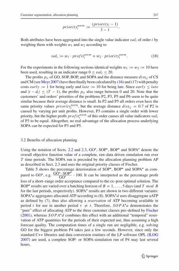
priori t ynormi := (priori t yi − 1)

3 − 1.

Both attributes have been aggregated into the single value indicator vali of order i byweighing them with weights w1 and w2 according to

vali := w1 · prof i tnormi + w2 · priori t ynorm

i . (18)

For the experiments in the following sections identical weights w1 := w2 := 10 havebeen used, resulting in an indicator range 0 ≤ vali ≤ 20.

The profits pit of GO, SOP, BOP, and SOPA and the distance measure disti j of CSand CM (see Meyr 2007) have then finally been calculated by (16) and (17) with penaltycosts early := 1 for being early and late := 10 for being late. Since early ≤ lateand |t − di | ≤ (T − 1), the profits pit also range between 0 and 20. Note that thecustomers’ and orders’ priorities of the problems P2, P3, P5 and P6 seem to be quitesimilar because their average distance is small. In P2 and P5 all orders even have thesame priority values priori t ynorm

i , but the average distance disti j = 0.7 of P2 iscaused by varying per unit profits. However, P3 contains a single order with lowerpriority, but the higher profit prof i tnorm

i of this order causes all value indicators valiof P3 to be equal. Altogether, no real advantage of the allocation process underlyingSOPA can be expected for P3 and P5.

3.2 Benefits of allocation planning

Using the notation of Sects. 2.2 and 2.3, GO�, SOP�, BOP� and SOPA� denote theoverall objective function value of a complete, raw-data driven simulation run overT time periods. The SOPA run is preceded by the allocation planning problem APas described in Sect. 2.3 and uses the original priority classes of Fischer.

Table 5 shows the percentage deterioration of SOP�, BOP� and SOPA� as com-

pared to GO�, e.g. GO�−SOP�

GO� · 100. It can be interpreted as the percentage profit

loss of a short–range order acceptance compared to the ex–post optimal solution. TheBOP� results are varied over a batching horizon of B = 1, . . . , 5 days (and T mod Bfor the last periods, respectively). SOPA� results are shown in two different variants:SOPA�a aggregates allocated ATP according to (8). SOPA�d uses disaggregate aATPas defined by (7), thus also allowing a reservation of ATP becoming available inperiod t for use in another period τ �= t . Therefore, SO P A�a demonstrates the“pure” effect of allocating ATP to the three customer classes pre–defined by Fischer(2001), whereas SO P A�d combines this effect with an additional “temporal” reser-vation of ATP quantities for the periods of their expected use, thus assuming a highforecast quality. The computation times of a single run are negligible, e.g. solvingGO for the biggest problem P4 takes just a few seconds. However, since only thestandard C++ libraries and data conversion routines of the LP software OPL (ILOG2007) are used, a complete SOP- or SOPA-simulation run of P4 may last severalhours.

123

248 H. Meyr

Table 5 Percentage profit loss of SO P�, B O P� (B = 1, . . . , 5) and SO P A� (disaggregate, aggregate)as compared to G O�

P1 P2 P3 P4 P5 P6 Average

SOP* 15.0 21.1 0.0 12.4 1.2 6.9 9.4

BOP*1 14.8 21.0 0.0 11.6 1.2 6.8 9.2

BOP*2 14.1 21.0 0.0 11.0 1.2 6.8 9.0

BOP*3 14.1 13.3 0.0 10.7 0.6 6.7 7.6

BOP*4 13.6 20.8 0.0 6.3 1.2 6.7 8.1

BOP*5 12.1 11.2 0.0 10.0 0.3 6.7 6.7

SOPA*a 5.5 21.1 0.0 1.5 1.2 0.3 4.9

SOPA*d 0.5 0.1 0.0 0.2 0.0 0.3 0.2

As expected, batching orders and increasing the batching horizon B is advantageouswhen compared to the FCFS single order processing SOP. But even for a batch horizonof a whole week, the overall improvement is rather disappointing. Astonishingly, thisholds especially true for the problems P4 and P6, which show a high degree of freedombecause of their large number of orders per day. Of course, a simulation horizon of 30days is actually too short for such experiments. However, studying Table 5 it seemslikely that increasing the simulation horizon would stabilize the results, but not reallychange the overall picture.

SOPA�a shows a significant improvement for problems P1, P4 and P6. The diffe-rence to SO P� is only caused by the allocation planning on basis of the three priorityclasses used by Fischer (see Sect. 3.1, Table 4). These results can further be improvedby SO P A�d, which allows a temporal reservation of ATP, too. In this case, near–optimal profits can be gained for all six scenarios. Thus, if companies are able torealize a high forecasting accuracy, defining disaggregate ATP seems reasonable.

SOP solves P3 and P5 almost to optimality because of their corresponding custo-mers’ homogeneity and the distances disti j = 0 between every two orders i and j . Theprofit loss of 1.2% for P5 is caused by inventory or backlogging costs as a consequenceof an unfavorable temporal assignment of ATP and can thus additionally be avoidedby SO P A�d. As opposite to P3 and P5, P2 not only shows a small number of orders,but also a non–zero heterogeneity. This might be the reason for the exorbitant advan-tage of temporal reservation for P2. On the other hand, temporal reservation seems tohave no impact on P6 (0.3 for both SOPA�a and SOPA�d). Summing up both SOPAvariants clearly profit from clustering effects.

3.3 Variation of the ATP search space and consumption rules

Both SOPA variants of the last section assumed that ATP can only be consumed in thepriority class classi(s), the order i(s) belongs to. The subsequent experiments allowa more flexible consumption of ATP by varying the ATP search space �i(s) in thefollowing way:

123


cc ⇔ ATP can only be consumed in the class classi(s), order i(s) has been assignedto, i.e. �i(s) := {classi(s)} (as done in Sect. 3.2).

cK ⇔ ATP can be consumed in the order’s original class or in classes with lowerpriority, i.e. �i(s) := {classi(s), . . . , K } (see Sect. 2.3 regarding the sorting ofclasses).

1K ⇔ ATP can be consumed in all classes, i.e. �i(s) := {1, . . . , K }.1c ⇔ ATP can be consumed in the order’s original class or in classes with higher

priority, i.e. �i(s) := {1, . . . , classi(s)}.Intuitively, the last variant does not seem to make much sense, but has been imple-mented for ease of validation and comparison.

Note that the constraints above do not specify a sequence for searching this space. Bysolving the SOPA model (9) – (12) using linear programming, ATP can be consumedfreely within the search space �i(s) because—for a given period t—the order’s originalprofit pi(s),t remains the same independently of the class, the ATP quantities actuallycome from. In order to guide the search through various priority classes in an intendedmanner (while still applying LP methods), fictitious gains and losses have been definedthe following way: The objective function (9) is extended by

∑

t,k≥classi(s)

(K − k) · 0.01 · pi(s),t oskt (19)

for the search space cK and by (19) plus

∑

t,k<classi(s)

(k − classi(s)) · 0.01 · pi(s),t oskt (20)

for the search space 1K. Thus, the allowed classes are searched in an order of descen-ding priorities first, starting with the original class classi(s). If no such ATP has beenfound for a search space 1K, higher priority classes are then searched in a sequenceof ascending priorities, starting with classi(s) − 1. Of course, the loss of profit shownin Table 6 has been calculated on basis of the regular profits (9), only. This way, ATPsearch rules, as proposed by Kilger and Meyr (2008) and Fischer (2001) and used inmost APS, can also be simulated within the LP framework of this paper.

Table 6 shows the percentage profit losses for a variation of aATP aggregation(aggregate, disaggregate), of the search space (cc, cK, 1K, 1c) and of the searchsequence (free allocation, search sequence predefined). The two rows marked in boldcorrespond to the respective SOPA� results of Table 5.

When comparing the four a/·/f scenarios among themselves, the best results areachieved for the cc search space, i.e. when staying within an order’s original priorityclass. Access to lower class ATP is only reasonable if search rules are used (a/cK/s).In this case, the a/cc/f results can be equalized but not improved. Free access to higherpriority ATP (a/1K/· and a/1c/f) is indeed proven to be nonsense. A variation of thesearch space or the introduction of search rules (a/·/·) do not show any effects on P2 andP5. For these products a profit increase can only be achieved by temporal reservation(d/·/·). The situation is actually the same for P3. Its anomalies for a/cK/· only occur

123

250 H. Meyr

Table 6 Percentage profit loss of SOPA� as compared to GO� for varying temporal reservation (aggregate,disaggregate), ATP search space (cc = original class, cK = lower priority, 1K = all classes, 1c = higherpriority) and ATP search rules (f = free allocation, s = search sequence predefined)

P1 P2 P3 P4 P5 P6 Averagea

a/cc/f 5.5 21.1 0.0 1.5 1.2 0.3 5.9

a/cK/f 5.5 21.1 (24.4) 4.3 1.2 0.3 6.5

a/1K/f 15.0 21.1 0.0 12.5 1.2 6.9 11.3

a/1c/f 18.0 21.1 0.0 18.9 1.2 6.9 13.2

a/cK/s 5.5 21.1 (17.7) 1.5 1.2 0.3 5.9

a/1K/s 15.0 21.1 0.0 12.4 1.2 6.9 11.3

d/cc/f 0.5 0.1 0.0 0.2 0.0 0.3 0.2

d/cK/f 0.5 0.1 0.0 0.2 0.0 0.3 0.2

d/1K/f 0.6 0.1 0.0 6.8 0.0 0.8 1.7

d/1c/f 12.8 0.1 0.0 13.8 0.0 0.8 5.5

d/cK/s 0.5 0.1 0.0 0.2 0.0 0.3 0.2

d/1K/s 0.6 0.1 0.0 6.8 0.0 0.8 1.7

a Without P3

because the penalty holding costs “early = 1” have turned out to be too low for thisproduct. Thus, the average values in the corresponding column of Table 6 have beencalculated without considering P3.

The comparison of the a/·/· with their respective d/·/· scenarios emphasizes theadvantages of a temporal reservation, again. Altogether the picture is similar for thedisaggregate scenarios. The search spaces cc and cK show equal quality, whereas 1Kand 1c compare badly. A positive effect of search rules cannot be recognized, here.

3.4 Variation of the number of classes

All SO P A� results presented so far are based on Fischer’s original assignment ofcustomers to three priority classes (see Sect. 3.1). It will now be investigated whethera variation of the number of priority classes might be advantageous. At the sametime the various ATP consumption alternatives will be compared again. The followingexperiments will be limited to P1. Product P1 has been chosen because

• it comprises only 37 orders and thus can be simulated in short computation times,• Fischer’s assignment of orders to classes showed balanced proportions for P1 (8/14/

15, see Table 4), and because• the SOPA allocation achieved significant and non–identical profit increases for both

variants—those with (0.5% loss) and those without (5.5%) temporal reservation—as compared to the standard SOP (15%) procedure (see Table 5).

Up to 20 priority classes have been generated using the clustering models and heuristicsof Meyr (2007). Table 7 shows the average of the corresponding percentage SOPA�

profit losses.

123


Table 7 Percentage profit loss of SOPA� as compared to G O� for P1 with respect to different ATPconsumption rules (see Table 6) and a varying number of priority classes K (missing entry = 0.0)

Reser.: Aggregate Disaggregate

Space: cc cK 1K 1c cK 1K cc cK 1K 1c cK 1K

Search: Free Sequ. Free Sequ.

K = 1 15.0 15.0 15.0 15.0 15.0 15.0 0.9 0.9 0.9 0.9 0.9 0.9

2 10.1 10.1 15.0 15.1 10.1 15.0 0.6 0.6 0.6 1.6 0.6 0.6

3 6.4 6.7 15.0 17.2 6.4 15.0 0.5 0.5 0.5 10.5 0.5 0.5

4 5.7 5.7 15.0 18.0 5.7 15.0 0.4 0.4 0.5 10.6 0.4 0.5

5 4.5 5.2 15.0 20.8 4.5 15.0 0.4 0.4 0.5 10.6 0.4 0.5

6 3.6 4.3 15.0 23.8 3.6 15.0 0.1 12.0 0.1

7 2.7 3.2 15.0 24.7 2.7 15.0 0.2 0.2 0.3 12.1 0.2 0.3

8 2.9 3.5 15.0 26.1 2.9 15.0 0.1 12.0 0.1

9 2.4 2.7 15.0 26.7 2.4 14.9 0.1 12.0 0.1

10 2.4 2.7 15.0 26.2 2.4 14.9 0.1 12.0 0.1

11 2.4 2.7 15.0 26.2 2.4 14.9 0.1 12.0 0.1

12 2.4 2.6 15.0 26.6 2.4 14.9 0.1 12.0 0.1

13 2.4 2.6 15.0 26.6 2.4 14.9 0.1 12.0 0.1

14 2.5 2.6 15.0 26.7 2.5 14.9 0.1 12.0 0.1

15 2.8 3.0 15.0 26.8 2.8 14.9 0.1 12.2 0.1

16 3.0 3.2 15.0 26.7 3.0 14.9 0.1 11.9

17 3.0 3.3 15.0 26.8 3.0 14.8 0.1 12.1

18 2.2 2.7 15.0 26.8 2.2 14.8 0.1 12.1

19 2.2 2.7 15.0 26.9 2.2 14.8 0.1 12.3

20 2.2 2.9 15.0 26.8 2.2 14.7 0.1 12.1

Average 4.05 4.38 15.0 24.0 4.05 14.9 0.16 0.16 0.24 10.7 0.16 0.20

Fischer 5.5 5.5 15.0 18.0 5.5 15.0 0.5 0.5 0.6 12.8 0.5 0.6

The row “average” of Table 7, containing average results of all 20 classes for eachATP search alternative, confirms the findings of the last section. Within the aggregateaATP scenarios (left part of Table 7) the search spaces cc and cK perform best again,also for a varying number of classes K . If access to lower priority classes is allowed(a/cK/·), sequential search rules should be applied instead of a free ATP consumption.The results of the disaggregate aATP (right part of Table 7) show a similar structure.However, the overall solution quality is better. Due to the limited degree of freedomleft after the temporal reservation, the d/1K/· scenarios also behave well. All in all,the a/cK/s–rules for ATP consumption, as proposed by most APS, seem justified bythese experiments. However, simply staying within the original class (a/cc/·) wouldperform equally.

The number of classes K appears more important than the search space and searchrule. This can be seen when studying the profit improvement resulting from increasingK for all ·/cc/· and ·/cK/· scenarios. The absurdity of an 1c search space becomes

123

252 H. Meyr

particularly clear in Table 7 where the profit loss even increases for a higher numberof customer classes. The row K = 1 shows the results for a single class only, i.e. theSOP performance without allocation planning. The a/·/· values coincide with the SOP�

value of P1 in Table 5. The d/·/· values for K = 1 illustrate the improvement possibleby solely introducing temporal reservation, without additionally building customerclasses. A profit loss of 0.9% still remains because all orders of the same period areconsidered as being equal. However, for P1 this affects only 2.1 orders on the average(see Table 4).

The two lines marked in italics allow a comparison of the clustering methods (K =3)of Meyr (2007) with the original customer segmentation of Fischer. There seemsto be a small advantage for the automatic methods. Nevertheless, in general bothsegmentations lead to similar results.

Note that the results are based on a single product only and thus can hardly be gene-ralized. Nevertheless, the example shows that profit can be increased by introducingpriority classes. Even if there is no obvious, natural customer segmentation, a cluste-ring into several price classes is valuable, as long as different customer orders showvarious per unit profits. Thus, it seems more important whether a clustering is donethan how it is done. To what extent this assumption is true will be further investigatedin the next section.

3.5 Effects of clustering on SOPA

Table 8 shows the percentage profit loss of single order processing after allocationplanning, as compared to the global optimization result G O�, for each of the clusteringalternatives MinMax, Sum-DE, Sum-TA and Sum-TS of Meyr (2007), individually (seeSect. 2.4). The results are presented for the products P1, P4 and P6 comprising thelargest number of orders (37, 1,305 and 509, respectively) and showing the largestinhomogeneity of distances disti j (see Table 3). For ease of clarity, the simulationhas been restricted to the single d/cK/s scenario, one of the best-performing scenariosof Sect. 3.4. Missing entries in the table indicate a profit loss of 0.00, i.e. that G O�

has been reached. Note that the MinMax results and the results of the CS heuristicsSum-DE, Sum-TA and Sum-TS would not have been directly comparable because theysolve the two different problems CM and CS. However, each product’s profit losses ofTable 8 can immediately be compared with each other, since the clustering heuristicsinfluence SOPA only indirectly by the different ways of cluster building.

Looking at row “aver.”, containing the results averaged over all 20 classes, givesa quick overview of the overall performance of the four heuristics. However, resultsappear nonuniform. While P1 and P6 are dominated by MinMax, the CS heuristics out-perform the CM algorithm clearly for P4. Thus there does not seem to be a significantcorrelation between the clustering objectives, the solution quality of different heuristicsand the profits generated by the respective clusters.

Interestingly, the profit losses of Sum-DE (for P6) and Sum-TA (for P4 and P6)decrease first, but then increase again. A reason for this might be found in a bad overallsolution quality of the CS heuristics, particularly for large problems with many ordersand classes (Meyr 2007). This is, besides forecast accuracy, a second argument forchoosing a not too large class number K .

123


Table 8 Percentage profit loss of the SOPA clustering alternatives MinMax (MM), Sum-DE, Sum-TA andSum-TS as compared to GO� for P1, P4 and P6 in the d/cK/s scenario (missing entry = 0.00)

K P1 P4 P6

MM DE TA TS MM DE TA TS MM DE TA TS

1 0.89 0.89 0.89 0.89 11.03 11.03 11.03 11.03 11.39 11.39 11.39 11.39

2 0.49 0.66 0.66 0.66 11.00 10.12 10.12 10.12 0.30 4.13 4.13 4.13

3 0.25 0.52 0.52 0.52 10.10 3.50 3.45 3.50 0.30 2.71 2.71 2.71

4 0.25 0.50 0.50 0.50 0.15 0.15 0.15 0.15 0.29 2.72 2.72 2.72

5 0.20 0.52 0.44 0.50 0.15 0.15 0.15 0.15 0.29 1.77 1.77 1.77

6 0.09 0.03 0.03 0.03 0.15 0.34 0.10 0.34 0.29

7 0.03 0.03 0.03 0.69 0.15 0.10 0.10 0.10 0.29

8 0.03 0.03 0.03 0.03 0.15 0.10 0.07 0.10 0.29

9 0.03 0.03 0.03 0.03 0.15 0.07 0.07 0.07 0.28

10 0.03 0.03 0.03 0.03 0.15 0.07 0.07 0.07 0.03

11 0.03 0.03 0.03 0.03 0.13 0.07 0.04 0.07 0.03

12 0.03 0.03 0.03 0.03 0.12 0.08 0.03 0.08 0.01 0.39

13 0.03 0.03 0.03 0.03 0.12 0.04 0.03 0.04 1.64

14 0.03 0.03 0.03 0.12 0.03 0.03 0.03 1.35

15 0.03 0.14 0.03 0.03 0.03 2.65

16 0.08 0.03 0.03 0.03 0.97 0.67

17 0.08 0.03 0.03 0.03

18 0.08 0.03 0.02 0.03 1.39 0.49

19 0.08 0.03 0.06 0.03 0.91

20 0.06 0.03 0.06 0.03 0.58 1.96

Aver. 0.12 0.17 0.16 0.20 1.71 1.30 1.28 1.30 0.69 1.58 1.34 1.14

The clustering of Fischer often shows better results (0.51 for P1, 0.21 for P4 and0.33 for P6) than the automatic clustering methods for K = 3. However, for K = 4already the MinMax clustering outperforms Fischer’s profits for all three products.Starting with K = 7 the same holds true for all CS heuristics as well. On the whole,all four heuristics show promising results when four or more classes are used.

Summing up this section, SOPA� indeed seems not to be very sensitive with respectto the clustering method used. An increase of the number of classes K leads to higherprofits if orders of the same product are inhomogeneous enough. Considering theexamples of this section at least 4, but better 6–7 classes should be used. However, thenumber of classes should not be chosen too large in order to reduce forecasting errorsand a bad performance of clustering heuristics, especially for CS.

4 Summary, managerial insights and outlook

The exemplary tests of the paper have shown that a first-come–first-served processingof arriving customer orders is hardly the best way of demand fulfillment in shortagesituations if reliable forecasts are available. Gathering data for a certain period of time

123

254 H. Meyr

and processing them in a batch can improve the situation. However, often customerservice sets a natural limit to such a procedure because customers increasingly expectshort order confirmation lead times. Another way of improvement can be to precedethe FCFS single order processing by a further allocation planning step. Here, priorityclasses for customer orders are built, available inventory (ATP quantities) is “allocated”to these classes and reserved for later consumption by their respective customers. Sucha customer segmentation has proven its potentials when introducing booking classes inairline yield management. Thus, the basic idea is not new and has also been supportedby advanced planning systems where simple ATP allocation and consumption rules areoffered. However, until now it was largely unclear—in science and practice—whether,when, why and to what extent such a proceeding might be useful in manufacturingindustries, too.

First answers to these questions have been given using an example from the lightingindustry where bulbs, fluorescent lamps etc. are made to stock on the basis of forecasts,first, and then sold from stock as soon as customer orders arrive. In order to demonstrateits potentials the following planning tasks had to be structured, discussed and solvedfirst:

1. Determination of a reasonable number of priority classes,2. clustering, i.e. assignment of customers and customer orders, respectively, to these

classes,3. allocation planning, i.e. allocation of available inventory on hand and planned

production quantities (ATP) to the priority classes, and4. ATP search, i.e. successively consuming this allocated ATP for each incoming

order. In this case both the search space (classes allowed) and the search sequencehave to be specified.

(1) has been tackled by means of simulation by varying the number of classes in areasonable range and (2) by applying standard clustering methods. For (3) and (4)linear programming models have been proposed and solved to optimality. All in all, itwas not intended to discuss each of these planning tasks in all detail and to solve it inthe best possible manner (even though this has not satisfactorily been done in scienceup to now). The primary goal was to bring all four tasks together in a single simulationexperiment to give an impression of the overall potential of allocation planning inmake–to–stock industries of this or similar types.

Since practical data have been used and the test bed was limited one has to be awarethat the results are only exemplary and more general statements would need furtherexperiments. Nevertheless, some interesting insights have been gained by the lightingexample and also common views have been confirmed: Introduction of priority classesand allocation planning can indeed increase revenues and profits, substantially. Themore heterogeneous the customers and their orders, e.g. with respect to the revenuesmade or to the strategic importance of the customers, the higher the advantages are.The number of customer classes plays an important role. Too few classes cause aloss of profits, too many classes make forecasting and clustering difficult. A temporalreservation of stocks, for use in a specific period, would generally be advantageous,but its practical application is only reasonable if customer demand can be forecastreliably enough.

123


At least in the lighting case, ATP consumption policies and the clustering methoditself are not as crucial as the choice of an appropriate number of classes. AlthoughLP methods have been applied for ATP consumption, simple ATP search rules wouldperform equally for this example. Such rules should either stay within an order’soriginal class or, as often claimed in Revenue Management and by APS, also allowaccess to lower priority classes. In the latter case, lower classes should better besearched for in order of descending priorities. However, note that LP methods or moresophisticated rules are required in more complex supply chains, e.g. in make-to-stocksupply chains with several stocking points and/or product substitution or in assemble-to-order supply chains with multi–stage bills of materials.

Thus, also in manufacturing industries managers should pay additional attention totheir customers’ varying nature and try to increase their overall customer service byallocating their scarce resources—in make–to–stock environments more specifically:their limited finished item stock—with higher priority to their more important cus-tomers. As the example of the lighting industry has shown, for this, not even activeor for the customer visible measures of customer segmentation (like fencing strate-gies or longer response times for order promises) are necessary. It is sufficient to takeadvantage of the already existing customer heterogeneity by applying standard clus-tering methods for identifying priority classes and by introducing well-coordinatedATP allocation and consumption processes.

Of course, there are still a lot of research challenges. Each of the planning tasksintroduced above should be investigated in more detail for prerequisites of applicationand fitting solution methods. First of all, the sensitivity of the results with respect toless reliable supply information, e.g. concerning the viability of production plans, anddemand information, i.e. to lower forecast accuracy, has to be tested. Furthermore,similar simulation experiments should be executed for more complex types of supplychains with other order penetration points. On the one hand, APS support allocationplanning and ATP consumption in resource- and capacity-constrained manufacturingindustries by offering the deterministic rules mentioned above. On the other hand,there is an obvious affinity to inventory rationing for several customer classes andto quantity-based revenue management, as defined by Talluri and Van Ryzin (2004)and practiced in many service industries like airline, hotel or car rental. Most of theirmethods are of a stochastic nature. Thus the most challenging prospect for futureresearch is to find out whether and how these worlds can learn from each other.

Acknowledgments The author is grateful to Markus E. Fischer and Bernhard Fleischmann for providingthe data, Matthias Mann for supporting the experiments and the Wiener Wissenschafts-, Forschungs- undTechnologiefonds (WWTF) for funding the research.

References

Ahuja R, Magnanti T, Orlin J (1993) Network flows: theory, algorithms and applications. Prentice Hall,Englewood Cliffs

Ball M, Chen C-Y, Zhao Z-Y (2004) Available to promise. In: Simchi-Levi D, Wu S, Shen Z-J (eds)Handbook of quantitative supply chain management: modelling in the eBusiness era. Kluwer, Bostonpp 447–482

123

256 H. Meyr

Chen C-Y, Zhao Z-Y, Ball M (2001) Quantity and due date quoting available to promise. Inform SystFrontiers 3(4):477–488

Chen C-Y, Zhao Z-Y, Ball M (2002) A model for batch advanced available–to–promise. Product OperManage 11(4):424–440

de Vericourt F, Karaesmen F, Dallery Y (2002) Optimal stock allocation for a capacitated supply system.Manage Sci 48(11):1486–1501

Dickersbach J (2004) Supply chain management with APO. Springer, BerlinFischer M (2001) Available-to-Promise: Aufgaben und Verfahren im Rahmen des Supply Chain Manage-

ment. S. Roderer Verlag, RegensburgFleischmann B, Meyr H (2003a) Customer orientation in Advanced Planning Systems. In: Dyckhoff H,

Lackes R, Reese J (eds) Supply Chain Management and Reverse Logistics. Springer, Berlin pp 297–321

Fleischmann B, Meyr H (2003b) Planning hierarchy, modeling and Advanced Planning Systems. In: deKok A, Graves S (eds) Supply chain management: design, coordination, operation, Vol 11 of handbooksin operations research and management science. Elsevier, Amsterdam pp 457–523

ILOG (2007) ILOG OPL development studio. URL: http://www.ilog.com/products/oplstudio/Keskinocak P, Tayur S (2004) Due-date management policies. In: Simchi-Levi D, Wu SD, Shen Z-J (eds)

Handbook of quantitative supply chain Analysis – Modeling in the E-Business era. Chap 12. Kluwer,Dordrecht pp 485–547

Kilger C, Meyr H (2008) Demand fulfilment and ATP. In: Stadtler H, Kilger C (eds) Supply Chain Mana-gement and Advanced Planning 4th edn, Chap 9. Springer, Berlin pp 181–198

Kilger C, Wetterauer U (2008) The selection process. In: Stadtler H, Kilger C (eds) Supply Chain Mana-gement and Advanced Planning 4th edn, Chap 16. Springer, Berlin pp 309–323

Knolmayer G, Mertens P, Zeier A (2002) Supply Chain Management based on SAP Systems. Springer,Berlin

Lee H, Padmanabhan V, Whang S (1997) The bullwhip effect in supply chains. Sloan Manage Rev Spring1997:93–102

Meyr H (2007) Clustering methods for rationing limited resources. Schriften zur Quantitativen Betriebswirt-schaftslehre 4/2007, Technische Universitaet Darmstadt, Hochschulstr. 1, 64289 Darmstadt, Germany

Meyr H, Rosic H, Seipl C, Wagner M, Wetterauer U (2008) Architecture of selected APS. In: Stadtler H,Kilger C (eds) Supply chain management and Advanced Planning 4th edn, Chap 18. Springer, Berlinpp 349–366

Meyr H, Wagner M, Rohde J (2008) Structure of advanced planning systems. In: Stadtler H, Kilger C (eds)Supply chain management and advanced planning 4th edn, Chap 5. Springer, Berlin pp 109–115

Pibernik R (2005) Advanced available–to–promise: classification, selected methods and requirements foroperations and inventory management. Int J Product Econ 93(94):239–252

Pibernik R (2006) Managing stock–outs effectively with order fulfilment systems. J Manufact TechnolManage 17(6):721–736

Quante R, Meyr H, Fleischmann M (2008) Revenue management and demand fulfilment: Matching applica-tions, models, and software. Technical report, Institute for Production Management, Vienna Universityof Economics and Business Administration, Nordbergstr. 15, 1090 Wien, Austria (OR Spectrum toappear)

Schneeweiss C (2003) Distributed decision making, 2nd edn. Springer, BerlinStadtler H, Kilger C (2008) Eds. Supply Chain Management and Advanced Planning, 4th edn. Springer,

BerlinTalluri K, Van Ryzin G (2004) The theory and practice of revenue management. Kluwer, Boston

123

http://www.ilog.com/pro ducts/oplstudio/

customer segmentation, allocation planning and order promising in make-to-stock production

Documents