customer-base concentration: implications for firm ... concentration: implications for firm...
TRANSCRIPT

Customer-base concentration:
Implications for firm performance and capital markets
Panos N. Patatoukas
Yale School of Management
Email: [email protected]
Tel: (203) 606-3740
This version: January 17, 2010
I gratefully acknowledge the guidance and encouragement from my dissertation committee
members: Brian Mittendorf, Shyam Sunder, Jake Thomas (Chair), and Frank Zhang. I also wish
to thank Rick Antle, Judith Chevalier, Ravi Dhar, Merle Ederhof, Alon Eizenberg, Roger
Ibbotson, Bige Kahraman, Myrto Kalouptsidi, Sang-Hyun Kim, Kalin Kolev, Stefan Lewellen,
Steven Malliaris, Nikolay Osadchiy, Philip Ostromogolsky, Ankur Pareek, Heather Tookes, Ari
Yezegel, Roy Zuckerman, and seminar participants at Yale School of Management, Athens
University of Economics & Business, the 9th
Trans-Atlantic Doctoral Conference at the London
Business School, the 6th
Accounting Research Workshop at the University of Bern, and the 2009
American Accounting Association Northeast Regional Meeting for their comments on earlier
versions. This paper is the recipient of the 2009 American Accounting Association Northeast
Region Best PhD Student Paper Award.

2
Customer-base concentration:
Implications for firm performance and capital markets
Abstract
In this paper, I examine whether and how customer-base concentration affects supplier firm
performance and stock market valuation. To this end, I compile a comprehensive sample of
supply chain relationships and introduce a measure, labeled CC, to capture the extent to which a
supplier‟s customer base is concentrated. In contrast to the conventional view of customer-base
concentration as an impediment to firm profitability, I document a positive contemporaneous
association between CC and accounting rates of return, which suggests that efficiencies accrue to
suppliers with concentrated customer bases. Consistent with a cause-and-effect link between
customer-base concentration and firm performance, analysis of intertemporal changes
demonstrates that CC increases predict efficiency gains in the form of reduced operating
expenses per dollar of sales and enhanced asset utilization. Using stock returns tests, however, I
find that investors systematically underreact to the implications of changes in customer-base
concentration for future firm fundamentals when setting stock prices. Over the thirty-year sample
period studied, a zero-investment trading strategy that exploits investors‟ underreaction yields
abnormal returns in the region of 10 percent per year.
Keywords: Customer-base concentration; DuPont profitability analysis; market efficiency.
JEL classification codes: M41; L25; G14.

3
1. Introduction
Relationships with major customers are conventionally considered to be an impediment
to supplier firm profitability. Reportedly, major customers pressure their dependent suppliers to
provide concessions such as lowering prices, extending trade credit, accelerating delivery times,
and carrying extra inventory. The popular press often highlights the “evils” of customer-base
concentration by reference to the case of Wal-Mart and its history of squeezing out every last
penny from its dependent suppliers (e.g., PBS Frontline 2004). However, research on
relationship marketing and operations management suggests that suppliers to major customers
may be able to achieve efficiencies in the form of decreased selling and administrative expenses,
and enhanced product distribution (e.g., Jackson 1985; Cowley 1988; Kalwani and Narayandas
1995). In addition, major customer relationships can foster information sharing along the supply
chain and help supplier firms streamline production and enhance working capital management
(e.g., Kalwani and Narayandas 1995; Kinney and Wempe 2002).
In this paper, I examine whether and how customer-base concentration affects supplier
firm performance and stock market valuation. To this end, I compile a comprehensive sample of
supply chain relationships in virtually all two-digit SIC industries over the thirty-year period
from 1977 to 2006, and introduce a measure to capture at the firm-year level the extent to which
a supplier‟s customer base is concentrated. My concentration measure, labeled CC, is an
application of the Herfindahl-Hirschman index and encompasses two elements of customer-base
diversification − namely, the number of major customers with which a supplier firm interacts and
the relative importance of each major customer in the firm‟s total revenue.
In contrast to the conventional view of major customer relationships, I find a positive
contemporaneous association between CC and accounting rates of return, which suggests that

4
suppliers with concentrated customer bases enjoy efficiencies. A detailed investigation of
operating performance drivers reveals that efficiencies accrue to more-concentrated suppliers in
the form of cost savings and enhanced working capital management. Specifically, more-
concentrated suppliers spend less on selling, general, and, administrative (SG&A) expenses per
dollar of sales, hold less inventory as a fraction of total assets, and experience higher inventory
turnover, as well as shorter cash conversion cycles. Accordingly, although more-concentrated
suppliers report lower gross margins, they experience higher operating profit margins and asset
turnover and, on the whole, tend to be more profitable.
A causal link between customer-base structure and performance implies that changes in
customer-base concentration are associated with changes in supplier firm performance. Indeed,
potential efficiency gains achieved through enhanced production coordination and inventory
management, cooperative advertising campaigns and marketing alliances with major customers,
are likely to flow gradually through a supplier‟s financial reporting system. To help assess the
existence of a causal link, I investigate the lead-lag association between changes in firm
performance and changes in customer-base concentration (ΔCC). Consistent with a cause-and-
effect relationship, I find that ΔCC is a strong leading indicator of one-year-ahead changes in
profit margins, asset turnover, and overall firm profitability. In particular, I find that increases in
customer-base concentration are subsequently followed by efficiency gains in the form of
reduced operating expenses per dollar of sales and enhanced asset utilization.
In order to address concerns of a spurious correlation between ΔCC and subsequent
changes in firm performance, I implement a two-stage regression approach. In the first stage, I
remove the component of ΔCC that is correlated with measurable characteristics of not only the
supplier firm but also of the supplier firm‟s customer base − including market capitalization,

5
book-to-market ratio, age, sales growth, distress risk, the number of reported business segments,
and product market share and competitiveness. In the second stage, I regress one-year-ahead
changes in firm profitability on the residual portion of ΔCC which is by construction orthogonal
to the characteristics considered. I find that residual ΔCC is a strong predictor of subsequent
changes in firm profitability; therefore, the lead-lag association between changes in firm
performance and changes in customer-base concentration is robust to spurious correlations.
Naturally, the question that emerges is to what extent investors use the forward-looking
information embedded in customer-base changes when setting stock prices. To address this
question, I employ annual-window association tests and find a significantly positive relationship
between ΔCC and inter-announcement stock returns. Additional analysis shows that ΔCC is
correlated with information not captured in reported accounting earnings and thus changes in
customer-base concentration are incrementally important in explaining stock returns.
Importantly, the positive sign of the association between ΔCC and contemporaneous stock
returns suggests that investors revise their beliefs and valuations in the direction of the
implications of customer-base changes for future firm performance. A related question is
whether investors are fully attentive to these implications when setting stock prices.
Bloomfield (2002) argues that limitations in investors‟ attention span can give rise to
stock market anomalies related to the forward-looking content of fundamental variables. The
setting examined here is no exception. Although stock prices react in year t to customer-base
concentration changes, future stock returns tests reveal that stock prices continue to drift over the
subsequent year in the direction of the initial change. An annual trading strategy that exploits this
pattern yields abnormal returns in the region of 10% per year. Multivariate regression analysis

6
further demonstrates that the predictive power of ΔCC is separate from that of previously
identified predictors of the cross-section of stock returns.
A thorough examination of alternative explanations makes it hard to reconcile stock-
return predictability based on ΔCC with the pricing of risk in efficient markets. In fact, the
evidence suggests that a plausible explanation is mispricing caused by investors‟ systematic
underreaction to the implications of changes in customer-base concentration for future firm
fundamentals. Consistent with this type of underreaction, I find that a disproportionate fraction
of the effect is clustered around subsequent earnings announcements dates. In addition, I
document that stock-return predictability tends to be stronger among firms that are a priori more
likely to be mispriced (e.g., firms with low analyst coverage and low institutional ownership).
The findings reported here have the potential not only to inform but also to redirect the
ongoing debate on the impact of major customers on supplier firm performance. This is the first
study to provide large-sample evidence on the association of customer-base concentration with
supplier performance at the firm level. This is also the first study to exploit the dynamics of
supplier firms‟ customer bases and implement lead-lag analyses that mitigate limitations inherent
in association tests of contemporaneous levels. My study not only establishes an important link
between customer-base structure and firm performance but also provides evidence of how
changes in customer-base structure lead subsequent changes in firm performance.
Overall, the evidence validates the relevance of disaggregated revenue disclosures for
financial statement analysis by demonstrating an economically important and statistically
significant link between customer-base concentration, firm fundamentals, and stock returns.
Accordingly, my study contributes to research on inter-organizational relationships and
intangibles as sources of firm value (e.g., Amir and Lev 1996; Lev 2001; Gosman, Kelly,

7
Olsson, and Warfield 2004). My findings also add to the growing evidence that investors
sometimes underreact to the forward-looking content of fundamental variables (e.g., Bernard and
Thomas 1990; Sloan 1996) and to the evolving literature on investors‟ limited attention to inter-
firm links (e.g., Menzly and Ozbas 2006; Cohen and Frazzini 2008).1 Finally, the inferences
drawn may be of interest to accounting standard setters who are currently considering ways to
revise the presentation of financial statements so as to provide improved disaggregated
information about firms‟ operations.2
The rest of the paper is organized as follows. Section 2 reviews related literature and
motivates the research questions. Section 3 describes the sample and provides descriptive
statistics. Section 4 examines the empirical link between customer-base concentration and firm
performance. Section 5 probes into the capital market implications of customer-base
concentration. Section 6 concludes and outlines directions for future research.
2. Background and research questions
The conventional view of customer-base concentration as an impediment to firm
performance can be traced at least as far back as the ideas of John Kenneth Galbraith on relative
bargaining power. In particular, J. K. Galbraith (1952) proposes that an important tactic in the
exercise of power consists in keeping the supplier in a state of uncertainty as to the intentions of
a major customer. The argument is that major customers often place orders around which the
production and investment of suppliers with concentrated customer bases become organized. A
1 Prior accounting research demonstrates that investors are not fully attentive to the forward-looking information
embedded in several fundamental variables, most notably earnings (e.g., Bernard and Thomas 1990) and earnings
components (e.g., Sloan 1996). Menzly and Ozbas (2006) use upstream and downstream definitions of industries
and present evidence of cross-industry price momentum. Similarly, Cohen and Frazzini (2008) find that the monthly
strategy of buying/selling firms whose customers had the most positive/negative returns in the previous month yields
abnormal returns, and argue that predictability is driven by investors‟ limited attention to inter-firm relations.
2 The latest updates regarding the joint project of the IASB and the FASB on “Financial Statement Presentation” can
be found at http://www.fasb.org/financial_statement_presentation.shtml.

8
shift in this practice imposes prompt and heavy losses, and thus the threat or even the fear of this
sanction is enough to provide customers with considerable bargaining power over transaction
prices and trade credit terms (Scherer 1970). In this spirit, Porter (1974) argues that “where
retailer power is high, the manufacturer's rate of return will be bargained down, ceteris paribus.”
Early research emphasizes the impact of customer power on supplier gross margins and,
consistent with the view that major customers exercise power vis-à-vis their relatively weaker
suppliers, finds that industry-level measures of customer bargaining power are associated with
lower supplier-industry gross margins (e.g., Lustgarten 1975; LaFrance 1979; Ravenscraft 1983).
However, Newmark (1989) shows that results of prior industry-level studies are misleading due
to measurement error in industry-level price-cost margins. Research extending the investigation
from the industry level to the firm level has also produced mixed results. To illustrate, on the one
hand, Galbraith and Stiles (1983) examine a sample of strategic business units of manufacturers
in the PIMS database and find that suppliers with diffused customer bases are associated with
higher operating profit margins. On the other hand, Kalwani and Narayandas (1995) report
higher levels of return on investment for a sample of 76 manufacturers in long-term relationships
with major customers.
These mixed findings have sparked an ongoing debate about the impact of customer
power on supplier profitability and, in fact, some argue that efficiencies may accrue to suppliers
with concentrated customer bases. In line with this argument, casual observation and academic
research in marketing and operations management suggest that increased customer-base
concentration may provide supplier firms with benefits, such as decreased cost of sales and
enhanced product distribution.3
3 As a real-life example, consider the case of Hasbro, Inc., one of the largest toy makers in the world. Hasbro
disclosed in its 2006 Annual Report the following information related to its customer base: “During 2006, sales to

9
For example, Jackson (1985) discusses how suppliers may be able to exploit their major
customers‟ reputations and brand names and use them as showcase accounts to attract other
customers. Cowley (1988) examines a sample of strategic business units in the PIMS database
for the years 1973-1976 and finds that selling and advertising costs tend to be lower when there
are fewer major customers to service. More recently, Kalwani and Narayandas (1995) propose
that manufacturers in long-term relationships with major customers are able to achieve cost
reductions in their SG&A expenses due to lower service costs, higher repeat sales and cross-
selling opportunities, and higher overall effectiveness of selling expenditures. In a similar vein,
Matsumura and Schloetzer (2009) argue that apparel industry suppliers can achieve cost savings
by engaging in collaborative marketing campaigns with their major customers.
A related stream of research in marketing and operations management proposes that
suppliers with concentrated customer bases can achieve enhancements in their working capital
management due to increased information sharing and improved production coordination along
the supply chain. In turn, increased production coordination can help concentrated suppliers
mitigate distortions common to supply chains (e.g., the bullwhip effect), reduce redesign costs,
and avoid delays in product development.4 Along these lines, recent empirical research provides
small-sample evidence that customer-supplier collaboration improves upstream inventory
management. Notably, Kalwani and Narayandas (1995) find that 76 manufacturers in long-term
relationships with major customers are able to reduce inventory holding and control costs.
our three largest customers, Wal-Mart Stores, Inc., Target Corporation, and Toys „R Us, Inc., represented 24%,
13%, and 11%, respectively, of consolidated net revenues, and sales to our top five customers accounted for
approximately 53% of our consolidated net revenues. While the consolidation of our customer base may provide
certain benefits to us, such as potentially more efficient product distribution and other decreased costs of sales and
distribution, increased customer concentration could also negatively impact our ability to negotiate higher sales
prices for our products and could result in lower gross margins than would otherwise be obtained if there were less
consolidation among our customers.”
4 The bullwhip effect (also known as “whiplash” or “whipsaw” effect) refers to the phenomenon where orders to the
supplier tend to have larger variance than sales to the customer (Lee, Padmanabhan, and Whang 1997).

10
Similarly, Matsumura and Schloetzer (2009) find enhanced inventory management capabilities
for a sample of 56 apparel industry suppliers with major customers. Case studies also illustrate
that partnerships between suppliers and their trusted major customers accelerate the deployment
of sophisticated procurement systems such as just-in-time (JIT) delivery (Kumar 1996).5
In summary, the results of industry-level studies are inconclusive, while those of firm-
level studies may not generalize to more representative samples, across industries, and over time.
Hence, the moment is ripe for an in-depth, large-sample study on the implications of customer-
base concentration for supplier firm performance. To this end, I compile a comprehensive
sample of 47,396 annual supplier-customer relations in virtually all two-digit SIC industries from
1977 to 2006, and introduce a measure to capture at the firm-year level the extent to which a
supplier‟s customer base is concentrated.
Specifically, the primary explanatory variable introduced in this study is firm i‟s
customer concentration (CC) in year t measured across the firm‟s J major customers, as
described below:
𝐶𝐶𝑖𝑡 = 𝑆𝑎𝑙𝑒𝑠𝑖𝑗 𝑡
𝑆𝑎𝑙𝑒𝑠𝑖𝑡
2𝐽
𝑗=1
(1)
where 𝑆𝑎𝑙𝑒𝑠𝑖𝑗𝑡 represents firm i‟s sales to major customer j in year t, and 𝑆𝑎𝑙𝑒𝑠𝑖𝑡 represents firm
i‟s total sales in year t. In essence, CC is an application of the Herfindahl-Hirschman index and
attempts to capture the extent to which a firm‟s customer base is more or less concentrated by
taking into account two elements of diversification: (i) the number of major customers with
5 Balakrishnan, Linsmeier, and Venkatachalam (1996) report for a sample of 46 JIT adopters that JIT-related
benefits (e.g., inventory turnover) are restricted to adopters with diffused customer bases (free adopters) and argue
that firms with concentrated customer bases (captive adopters) may be adopting JIT manufacturing to countervail
the adverse effects of price concessions to their major customers. However, Kinney and Wempe (2002), using an
extended sample of 201 JIT adopters, report no difference in the retention of JIT-related benefits across captive and
free adopters and argue that firms with concentrated customer bases enjoy lower downstream coordination costs.

11
which the firm interacts, and (ii) the relative importance of each major customer in the firm‟s
total revenue.6 The theoretical range of CC is between 0 and 1, where lower values correspond to
less concentrated customer bases and higher values correspond to more concentrated ones.
In the first part of my empirical analysis, I investigate whether and how efficiencies
accrue to suppliers with concentrated customer bases by testing the association of CC with
contemporaneous firm profitability and profitability drivers. However, contemporaneous
association tests provide little basis for inferring causality. To help assess whether a causal
relationship may exist between CC and firm performance, I investigate the lead-lag association
between changes in firm performance and changes in customer-base concentration (ΔCC). The
idea underlying the intertemporal analysis is that potential efficiency gains achieved through
enhanced production coordination and inventory management, cooperative advertising
campaigns and marketing alliances with major customers are likely to flow gradually through a
supplier‟s financial reporting system. Hence, a causal link between customer-base structure and
performance implies that changes in customer-base concentration are associated with subsequent
changes in supplier firm performance.
In the second part of my analysis, I investigate the extent to which investors incorporate
fundamental information embedded in ΔCC when setting stock prices. In the spirit of Ball and
Brown (1968), I examine the association between ΔCC and contemporaneous stock returns.
Establishing statistical significance would suggest that the information in ΔCC is correlated with
information that is value-relevant to stock market participants. In future returns tests, I set up a
6 The measurement of diversification is central to the empirical investigation of the implications of customer-base
concentration for firm performance. All results reported in this study are robust to the following alternative CC
measures: (i) 𝐶𝐶𝑖𝑡 =1
𝐽
𝑆𝑎𝑙𝑒𝑠 𝑖𝑗𝑡
𝑆𝑎𝑙𝑒𝑠 𝑖𝑡
𝐽𝑗=1 , and (ii) 𝐶𝐶𝑖𝑡 =
𝑆𝑎𝑙𝑒𝑠 𝑖𝑗𝑡
𝑆𝑎𝑙𝑒𝑠 𝑖𝑡
2𝐽𝑗=1
𝑆𝑎𝑙𝑒𝑠 𝑖𝑗𝑡
𝑆𝑎𝑙𝑒𝑠 𝑖𝑡
𝐽𝑗=1 .

12
zero-investment trading strategy designed to exploit forward-looking information in ΔCC. If this
information is not fully reflected in current prices, then this strategy can earn abnormal returns.
3. Sample and descriptive analysis
The sample formation is based on FASB‟s and SEC‟s requirements that public firms
disclose the amount of revenue derived from each major customer.7 This information is available
in the COMPUSTAT Segment Files. The COMPUSTAT Segment Files provide the type and
name of a major customer along with the dollar amount of annual revenues generated from each
major customer.
I employ a phonetic string algorithm to match each customer name to the corresponding
identifying gvkey code of one of the companies listed in the COMPUSTAT Annual Files.
Following the automated phonetic matching, I inspect every match to ensure accuracy and
manually correct inaccurate and missing matches by hand-collecting information from the
COMPUSTAT database and the EDGAR database. Next, I combine the initial sample of
supplier-customer links with accounting data from the annual COMPUSTAT files and stock
returns data from the monthly CRSP files. Given that suppliers and customers may or may not
share the same fiscal year-end, I match each supplier with the most recent customer information
as of the month corresponding to the supplier‟s fiscal year-end.
7 Major customer disclosure requirements were initially established by the Statement of Financial Accounting
Standards No. 14 (SFAS 14) issued by the FASB in 1976. The requirement was amended in 1979 by SFAS 30 and
both SFAS 14 and SFAS 30 were superseded by SFAS 131 in 1997. More specifically, SFAS 14 §39 stipulates that
“if 10% or more of the revenue of an enterprise is derived from sales to any single customer, that fact and the
amount of revenue from each such customer shall be disclosed.” SFAS 131 §39 reiterates that “if revenues from
transactions with a single external customer amount to 10% or more of an enterprise‟s revenues, the enterprise shall
disclose that fact, the total amount of revenues from each such customer and the identity of the segment or segments
reporting the revenues.” Similar disclosure requirements are set by Regulation S-K of the SEC. Specifically, Item
101 (§c, vii) specifies that “the name of any customer and its relationship, if any, with the registrant or its
subsidiaries shall be disclosed if sales to the customer by one or more segments are made in an aggregate amount
equal to 10% or more of the registrant's consolidated revenues and the loss of such customer would have a material
adverse effect on the registrant and its subsidiaries taken as a whole.”

13
For a firm-year to be included in the sample it must have non-missing information about
customer concentration (CC), market value of equity (MV), profit margin measured as the ratio
of income before extraordinary items to net sales (PM), and asset turnover measured as the ratio
of net sales to the book value of total assets (ATO). To allow for a clear ranking of performance
and facilitate comparison with prior studies on firm profitability (e.g., Fairfield and Yohn 2001;
Soliman 2008), firm-years with negative profit margins are excluded. To further mitigate the
impact of distressed stocks, I exclude firm-years with negative book value of equity.8
The procedures and criteria described above yield a sample of 47,396 supplier-customer
relations for a total of 26,246 unique supplier firm-years from 1977 to 2006. Note that my
sample of unique supplier firm-years covers as much as 25.5% of the COMPUSTAT universe.
Observations are grouped based on the calendar year t corresponding to the fiscal year-end
month.
Since suppliers often disclose multiple major customers, for each of the financial
characteristics of supplier i‟s J major customers in year t I construct a weighted-average index
(CVAR) as follows:
𝐶𝑉𝐴𝑅𝑖𝑡 = 𝑤𝑖𝑗𝑡 × 𝐶𝑉𝐴𝑅𝑖𝑗𝑡
𝐽
𝑗=1
(2)
The weight 𝑤𝑖𝑗𝑡 is defined as 𝑆𝑎𝑙𝑒𝑠 𝑖𝑗𝑡
𝑆𝑎𝑙𝑒𝑠 𝑖𝑡
𝑆𝑎𝑙𝑒𝑠 𝑖𝑗𝑡
𝑆𝑎𝑙𝑒𝑠 𝑖𝑡
𝐽𝑗=1 , where 𝑆𝑎𝑙𝑒𝑠𝑖𝑗𝑡 is firm i‟s sales to major
customer j in year t and 𝑆𝑎𝑙𝑒𝑠𝑖𝑡 represents firm i‟s total sales in year t. To illustrate, 𝐶𝑀𝑉𝑖𝑗𝑡 is
the market value of supplier i‟s major customer j in year t and 𝐶𝑀𝑉𝑖𝑡 is the weighted-average
8 As an empirical matter, all inferences drawn in my paper are robust to the inclusion of firms with negative profit
margins and negative book value of equity. Also note that financial services firms (SIC codes 60-69) are included in
the sample and that all my results are insensitive to the exclusion of these firms.
14
market value of supplier i‟s J major customers in year t. A drawback of this index is that it is
measured only across major customers that can be identified on the COMPUSTAT Annual files.
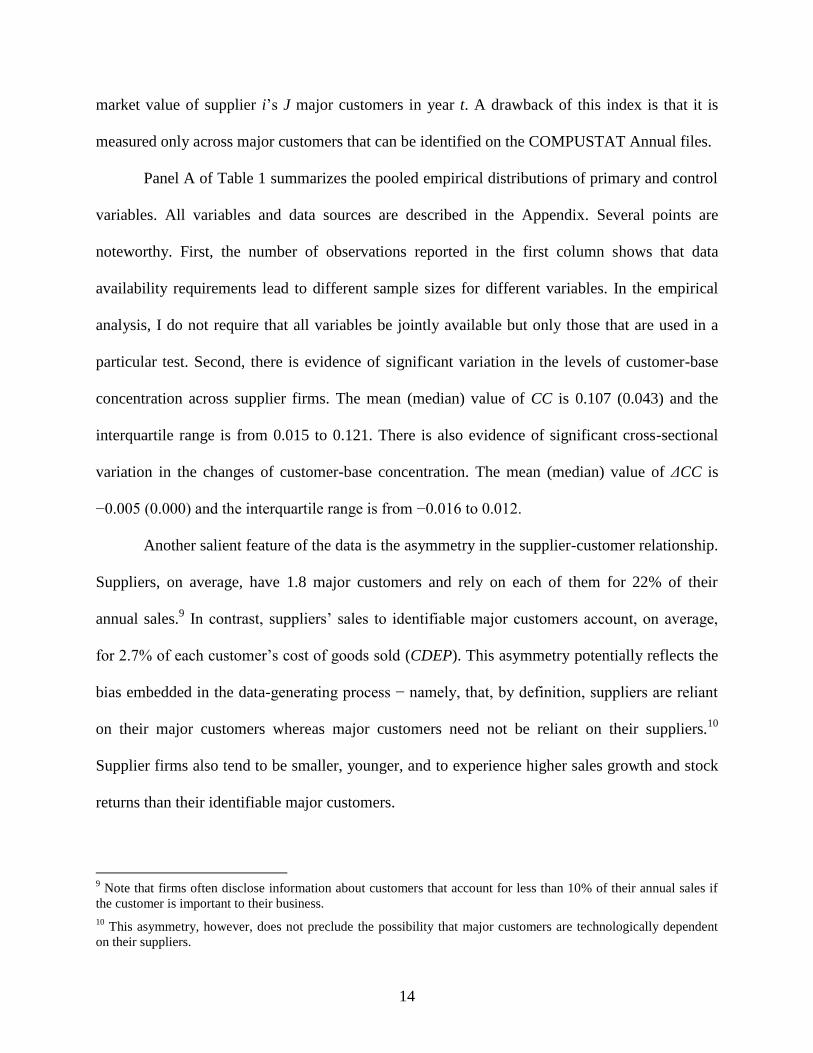
Panel A of Table 1 summarizes the pooled empirical distributions of primary and control
variables. All variables and data sources are described in the Appendix. Several points are
noteworthy. First, the number of observations reported in the first column shows that data
availability requirements lead to different sample sizes for different variables. In the empirical
analysis, I do not require that all variables be jointly available but only those that are used in a
particular test. Second, there is evidence of significant variation in the levels of customer-base
concentration across supplier firms. The mean (median) value of CC is 0.107 (0.043) and the
interquartile range is from 0.015 to 0.121. There is also evidence of significant cross-sectional
variation in the changes of customer-base concentration. The mean (median) value of ΔCC is
−0.005 (0.000) and the interquartile range is from −0.016 to 0.012.
Another salient feature of the data is the asymmetry in the supplier-customer relationship.
Suppliers, on average, have 1.8 major customers and rely on each of them for 22% of their
annual sales.9 In contrast, suppliers‟ sales to identifiable major customers account, on average,
for 2.7% of each customer‟s cost of goods sold (CDEP). This asymmetry potentially reflects the
bias embedded in the data-generating process − namely, that, by definition, suppliers are reliant
on their major customers whereas major customers need not be reliant on their suppliers.10
Supplier firms also tend to be smaller, younger, and to experience higher sales growth and stock
returns than their identifiable major customers.
9 Note that firms often disclose information about customers that account for less than 10% of their annual sales if
the customer is important to their business.
10 This asymmetry, however, does not preclude the possibility that major customers are technologically dependent
on their suppliers.

15
At this point it may be useful to highlight that approximately 79% of the supplier-
customer relations are between firms in different two-digit SIC industries, consistent with the
fact that supply chain relations tend to develop across sectors. In addition, industry clustering is
unlikely to inhibit the analysis since there is a substantial degree of representation of the sample
firms across as many as 69 two-digit SIC industries. The three most represented industries are
Electronic & Other Electrical Equipment & Components, Except Computer Equipment (36),
Business Services (73), and Industrial & Commercial Machinery & Computer Equipment (35).
These industries collectively account for roughly 30% of the total number of observations.11
Panel B of Table 1 reports Pearson and Spearman pair-wise correlations across variables.
The correlations of CC with firm characteristics imply that firms with more concentrated
customer bases tend to be smaller and younger, and to report higher sales growth. The positive
correlation between CC and ΔCC is consistent with mean-reversion in the levels of customer-
base concentration. Some preliminary findings are in order. First, the positive and significant (at
the 1% level) correlation of CC with ROA suggests that suppliers with more concentrated
customer bases tend to be more profitable. Second, the positive and significant (at the 1% level)
correlation between ΔCC and 𝛥𝑅𝑂𝐴𝑡+1 is consistent with an intertemporal association between
changes in customer-base concentration and supplier firm performance.
Lastly, Figure 1 examines time-series variation in the aggregate levels of customer-base
concentration. At the aggregate level, CC rises from 1977 to 1984, remains relatively stable
during the period leading to the enforcement of SFAS 131 in the end of 1997, and rises in the
post-1998 period. Consistent with an overall increasing trend in concentration, a regression of
the annual values of aggregate CC on time yields a positive and significant (at the 1% level)
11
My results are robust to the exclusion of supplier firms in the three most represented two-digit SIC industries.

16
estimated slope coefficient. Given that over the sample period studied COMPUSTAT has
expanded coverage of small firms, the increasing trend in CC may be an in-sample phenomenon
that is not necessarily reflective of macroeconomic trends.12
4. Customer-base concentration and firm performance
In this section, I investigate the empirical link between customer-base concentration and
supplier firm performance. The analysis proceeds in two steps. First, I examine the association of
the levels of customer-base concentration (CC) with supplier firm performance. Next, I exploit
the changes in customer-base concentration (ΔCC) and conduct lead-lag analyses that help assess
the existence of a cause-and-effect relationship between customer-base structure and supplier
firm performance.
4.1 Levels analysis
The conventional view of customer-base concentration as an impediment to supplier firm
performance emphasizes the impact of customer power on supplier gross margins. On the other
hand, research on relationship marketing and operations management argues that suppliers with
concentrated customer bases may achieve efficiencies in the form of lower marketing and
administrative expenses, higher asset utilization, and enhanced working capital management
capabilities. However, such efficiencies are unlikely to be reflected in suppliers‟ gross margins.
When compared to gross margins, accounting rates of return are deemed to measure overall firm
performance in a more comprehensive manner.
12
Consolidation trends in downstream industries are likely to constitute yet another source of time-series variation
in the aggregate levels of customer-base concentration. To see this point, note that consolidation in downstream
industries is likely to lead to a reduction in the number of downstream firms and, in turn, an increase in the
customer-base concentration of upstream firms. Indeed, Figure 1 shows that, at the aggregate level, CC increases
during the M&A waves of the mid-1980s and late-1990s.

17
In what follows, I investigate the empirical association between customer-base
concentration and accounting rates of return. Specifically, I estimate annual cross-sectional
regressions of the following form:
𝑃𝐸𝑅𝐹𝑂𝑅𝑀𝐴𝑁𝐶𝐸𝑖𝑡 = 𝛼𝑡 + 𝛽1𝑡𝐶𝐶𝑖𝑡 + 𝛽𝑘𝑡𝐶𝑖𝑡𝑘
𝐾
𝑘=2
+ 휀𝑖𝑡
(3)
The dependent variable in Equation (3) is firm performance as measured by return on assets
(ROA) and return on equity (ROE). ROA is the ratio of income before extraordinary items to the
book value of total assets, and ROE is the ratio of income before extraordinary items to the book
value of shareholders‟ equity.13
To understand the association of CC with profitability drivers, I decompose overall firm
profitability as 𝑅𝑂𝐴 =𝐼𝑛𝑐𝑜𝑚𝑒 𝐵𝑒𝑓𝑜𝑟𝑒 𝐸𝑥𝑡𝑟𝑎𝑜𝑟𝑑𝑖𝑛𝑎𝑟𝑦 𝐼𝑡𝑒𝑚𝑠
𝑁𝑒𝑡 𝑆𝑎𝑙𝑒𝑠×
𝑁𝑒𝑡 𝑆𝑎𝑙𝑒𝑠
𝑇𝑜𝑡𝑎𝑙 𝐴𝑠𝑠𝑒𝑡𝑠. The ratio of income before
extraordinary items to net sales measures profit margin (PM), while the ratio of net sales to total
assets measures asset turnover (ATO). This multiplicative decomposition, commonly known as
DuPont profitability analysis (see, e.g., Palepu, Healy, and Bernard 2004), is considered a useful
tool of financial statement analysis (Soliman 2008).14
Note that
𝑅𝑂𝐸 = 𝑅𝑂𝐴 ×𝑇𝑜𝑡𝑎𝑙 𝐴𝑠𝑠𝑒𝑡𝑠
𝑆𝑎𝑟𝑒 𝑜𝑙𝑑𝑒𝑟𝑠 ′𝐸𝑞𝑢𝑖𝑡𝑦, where the ratio of total assets to shareholder‟s equity
measures financial leverage.
The primary independent variable is CC as defined in Equation (1). Following prior
literature on the impact of buyer bargaining power on supplier firm performance (e.g., Kelly and
Gosman 2000), the vector of control variables (𝐶𝑘 ) includes the log of market capitalization
(MV), the log of firm age (AGE), sales growth (SG), financial leverage (FLEV), the number of
13
All my results hold after adjusting income for extraordinary items.
14 Soliman (2008) comprehensively explores the DuPont components and finds that the decomposition provides
useful information to market participants.

18
reported business segments (NSEG), and the Herfindahl-Hirschman index of the degree of
product market competition in the firm‟s industry (HHI). Industry dummies based on two-digit
SIC codes are included as additional regressors to control for industry fixed effects.
Table 2 reports the time-series means of the estimated coefficients. Statistical inference is
based on Fama-MacBeth (1973) t-statistics corrected for serial correlation using the Newey-West
(1987) adjustment with three lags.15
Columns 1 and 2 document the empirical association
between CC and overall firm profitability. After controlling for other firm characteristics, I find a
positive and significant (at the 1% level) association between CC and accounting rates of return.
The t-statistics for the coefficient estimates on CC are 9.47 and 5.00 for the ROA and ROE
models, respectively. Ceteris paribus, a one-standard-deviation increase in CC would increase
the mean value of accounting rates of return by 5%. Columns 3 and 4 examine separately the
association of CC with the two multiplicative components of overall firm performance. The
coefficient estimates reveal that CC is positively and significantly (at the 1% level) associated
with both asset turnover and profit margin.
To elucidate the association of CC with profit margin, I decompose income before
extraordinary items into operating income before depreciation and “other items.”16
Based on this
income decomposition, I break down profit margin into two additive components as 𝑃𝑀 =
𝑂𝑝𝑒𝑟𝑎𝑡𝑖𝑛𝑔 𝐼𝑛𝑐𝑜𝑚𝑒 𝐵𝑒𝑓𝑜𝑟𝑒 𝐷𝑒𝑝𝑟𝑒𝑐𝑖𝑎𝑡 𝑖𝑜𝑛
𝑁𝑒𝑡 𝑆𝑎𝑙𝑒𝑠+
𝑂𝑡𝑒𝑟 𝐼𝑡𝑒𝑚𝑠
𝑁𝑒𝑡 𝑆𝑎𝑙𝑒𝑠.17
The first component measures operating
15
All empirical tests reported in this paper are based on annual cross-sectional regressions and Fama-MacBeth
(1973) t-statistics corrected for serial correlation using the Newey-West (1987) adjustment. In unreported sensitivity
analysis, I repeat the entire study using pooled sample estimations and obtain similar results. In particular, I estimate
the models described in Equations (3) through (11) using pooled cross-sectional regressions with year and industry
fixed effects, and calculate t-statistics based on standard errors clustered by industry and year.
16 Note that “other items” capture all income statement line items that fall below operating income before
depreciation and above income before extraordinary items, including depreciation and amortization, interest
expense, non-operating income, special items, income taxes, and minority interest.
17 See Nissim and Penman (2001) for more details on profit margin decompositions.

19
margin (OM) and the second one measures non-operating margin (NOM). Columns 5 and 6
examine the association of CC with operating and non-operating margins. The finding here is
twofold. First, CC is positively and significantly (at the 1% level) associated with operating
margin (t-statistic = 4.74). Second, the association between CC and non-operating margin is
positive, albeit not significant at conventional levels. Therefore, operating margins are primarily
driving the positive association of CC with profit margins.
By definition, operating income before depreciation is equal to net sales minus cost of
goods sold and SG&A expenses. Accordingly, operating margin can be further decomposed into
gross margin minus the ratio of SG&A expenses to net sales or
𝑂𝑀 =𝑁𝑒𝑡 𝑆𝑎𝑙𝑒𝑠 −𝐶𝑜𝑠𝑡 𝑜𝑓 𝐺𝑜𝑜𝑑𝑠 𝑆𝑜𝑙𝑑
𝑁𝑒𝑡 𝑆𝑎𝑙𝑒𝑠−
𝑆𝐺&𝐴 𝑒𝑥𝑝𝑒𝑛𝑠𝑒𝑠
𝑁𝑒𝑡 𝑆𝑎𝑙𝑒𝑠.
Column 7 investigates the relationship between CC and gross margins (GM). The
coefficient on CC is negative and significant (at the 1% level) with t-statistic = −6.08. Consistent
with prior research on the impact of customer power on suppliers‟ gross margins (e.g., Kelly and
Gosman 2000), the negative association between CC and GM implies that more-concentrated
suppliers tend to report higher cost of goods sold per dollar of sales. The magnitude of the
estimated coefficient implies that, ceteris paribus, a one-standard-deviation increase in CC would
decrease the mean value of gross margins by 3%. This finding, however, is in sharp contrast with
evidence of a positive association between customer-base concentration and operating margins.
Therefore, the key implication is that more-concentrated suppliers enjoy higher operating
margins in spite of the fact that they report lower gross margins.
In turn, higher operating margins can be reconciled with lower gross margins only if
more-concentrated suppliers spend less on SG&A expenses per dollar of sales. Consistent with
this claim, the estimates reported in Column 8 imply that more-concentrated suppliers tend to

20
report significantly lower SG&A-to-sales ratios. The t-statistics for the coefficient estimate on
CC is −9.13 (significant at the 1% level). To gauge the magnitude of the coefficient estimate,
consider that a one-standard-deviation increase in CC would ceteris paribus decrease the mean
value of SG&A expenses per dollar of sales by more than 7%. Importantly, the association of CC
with SGA is strong enough to outweigh that between CC and GM and, in turn, to explain why
more concentrated suppliers experience higher operating margins than less concentrated ones.
At this juncture some robustness checks are in order. To address potential non-linearities
in the relation between firm performance and the explanatory variables, I re-estimate Equation
(3) using decile rank transformations of the right-hand side variables and find consistent results.
As an additional check, I repeat the analysis separately for each two-digit SIC industry, using
industry-by-industry pooled regressions with year fixed effects, and find that my results are not
sensitive to whether Equation (3) is estimated cross-sectionally or separately for each industry.18
Overall, the evidence supports that suppliers with more concentrated bases tend to be
more profitable because of efficiency gains in the form of enhanced asset utilization and reduced
SG&A spending per dollar of revenue earned. Next, I probe deeper into how these gains accrue
to more concentrated suppliers. To this end, I estimate the following annual cross-sectional
regression model:
𝐸𝐹𝐹𝐼𝐶𝐼𝐸𝑁𝑇𝑖𝑡 = 𝛼𝑡 + 𝛽1𝑡𝐶𝐶𝑖𝑡 + 𝛽𝑘𝑡𝐶𝑖𝑡𝑘
𝐾
𝑘=2
+ 휀𝑖𝑡
(4)
The dependent variable in Equation (4) measures a wide array of operating performance drivers.
The first set of variables focuses on inventory management and examines inventory turnover
(ITO) and inventory held as a fraction of total assets (IHLD). The second set considers the cash
18
I estimate industry-by-industry regressions using a pooled specification to ensure sufficient degrees of freedom for
each regression.

21
conversion cycle (CACC) and its components to gauge overall working capital management
efficiency.19
The right-hand side variables in Equation (4) are defined as before. Industry
dummies based on two-digit SIC codes are included to control for industry fixed effects. Results
from estimating Equation (4) are presented in Table 3.
Columns 1 and 2 test the association between CC and inventory management. I find that
CC is positively associated with inventory turnover and negatively associated with inventory
held as a fraction of total assets. The t-statistics on the estimated coefficients are large and
significant (at the 1% level), while the sign of the estimated coefficients implies that more-
concentrated suppliers experience higher inventory turnover and hold less inventory as a fraction
of total assets. To illustrate, a one-standard-deviation increase in CC would ceteris paribus
increase the mean value of inventory turnover by 13% and decrease the mean value of inventory
held per dollar of total assets by 5%.
Next, Column 3 documents a significantly positive association between CC and overall
working capital management efficiency as proxied by the cash conversion cycle.20
Columns 4
through 6 delve further into the association of CC with cash conversion cycle components.
Contrary to the view that major customers use their power to extract trade credit provisions from
their dependent suppliers (e.g., Scherer 1970), I do not find any systematic differences in the
receivables conversion cycles (RCP) of more-concentrated suppliers and less-concentrated ones.
In fact, more-concentrated suppliers tend to experience significantly longer payables conversion
periods (PCP) − as if they are able to extract extended trade credit provisions from their own
19
The cash conversion cycle (CACC) is defined as the inventory conversion period (ICP) plus the receivables
conversion period (RCP) minus the payables conversion period (PCP). ICP represents the efficiency of production
and inventory management, RCP measures a firm‟s ability to manage its downstream supply chain, and PCP
indicates the efficiency of upstream supply chain management,
20 Note that shorter cash conversion cycles indicate higher working capital management efficiency.

22
vendors − and shorter inventory conversion periods (ICP). The combination of these effects
induces an overall negative association between CC and cash conversion cycles.
Interestingly, the estimates reported in Column 7 reveal a negative and significant (at the
5% level) association between CC and provisions for doubtful accounts as a fraction of all
receivables (DOUBT). Stated otherwise, even though there is no systematic link between
customer-base concentration and trade credit provisions in the form of accounts receivable, the
collectibility of these receivables tends to be higher among more-concentrated suppliers.
To gain further insights, I also examine the association of CC with two salient line items
under SG&A – namely, advertising expenses per dollar of sales (ADV) and R&D expenses per
dollar of sales (RD). As a caveat, note that only a subsample of firms report advertising and
R&D expenses as separate line items. In my tests, I do not treat missing values but the inferences
drawn are not sensitive to whether or not I set missing values for advertising and R&D expenses
to zero.
In Column 8, I document a negative and significant (at the 1% level) association between
CC and ADV. In additional analysis (not reported for brevity), I find that subtracting advertising
expenses from SG&A expenses does not affect dramatically the magnitude and statistical
significance of the negative association between CC and SGA. Hence, cost savings in terms of
advertising expenses are only one of the reasons why more concentrated suppliers tend to report
higher operating margins than less concentrated ones.
Somewhat surprisingly, Column 9 reveals a positive and significant (at the 1% level)
association between CC and RD. In other words, suppliers with more concentrated customer
bases tend to spend more on R&D expenses per dollar of sales. This result is interesting for at
least two reasons. First, it implies that, in effect, R&D spending attenuates the overall negative

23
association between customer-base concentration and SG&A spending. Second, it provides a
new piece of evidence on how inter-firm relationships may foster innovativeness along the
supply chain.21
To summarize, the results reported in Tables 2 and 3 deliver a coherent message.
Although more-concentrated suppliers report lower gross margins, they spend less on SG&A and
advertising expenses per dollar of sales, hold less of their assets in inventory, as well as enjoy
higher inventory turnover and shorter cash conversion cycles. Accordingly, more-concentrated
suppliers experience not only higher operating and profit margins but also higher asset turnover
and, on the whole, tend to be more profitable.
4.2 Intertemporal changes analysis
A causal link between customer-base structure and performance implies that changes in
customer-base concentration are associated with changes in supplier firm performance. Indeed,
potential efficiency gains achieved through enhanced production coordination and inventory
management, cooperative advertising campaigns and marketing alliances with major customers,
are likely to flow gradually through a supplier‟s financial reporting system. Thus, a cause-and-
effect relationship predicts an intertemporal association between changes in customer-base
concentration and changes in supplier firm performance.
To help assess the existence of a causal link, I exploit the non-static nature of supplier
firms‟ customer bases and examine whether changes in customer-base concentration (ΔCC)
predict future changes in supplier firm performance. In particular, I estimate annual cross-
sectional regressions of the following form:
21
Several authors argue that the presence of trust in major customer relationships reduces the probability of
opportunistic behavior by any partner and increases the likelihood of customers and suppliers making relationship-
specific investments in specialized physical and human capital and intangibles such as R&D (see, e.g., Panayides
and Venus Lun 2009 and the references therein).

24
𝛥𝑃𝑅𝑂𝐹𝐼𝑇𝑖𝑡+1 = 𝛼𝑡 + 𝛽1𝑡𝛥𝐶𝐶𝑖𝑡 + 𝛽2𝑡𝑅𝑂𝐴𝑖𝑡 + 𝛽3𝑡𝛥𝑃𝑀𝑖𝑡 + 𝛽4𝑡𝛥𝐴𝑇𝑂𝑖𝑡 + 휀𝑖𝑡+1 (5)
The dependent variable in Equation (5) is the annual change in firm profitability between t and
t+1 measured relative to accounting rates of return. The primary independent variable is ΔCC
and it is defined as the annual change in customer-base concentration between t-1 and t. The set
of control variables is measured in t and includes the level of ROA and the changes in the
components of ROA − namely, changes in profit margins (ΔPM) and asset turnover (ΔATO).22
Industry dummies based on two-digit SIC codes are included to control for industry fixed effects.
Table 4 reports results from estimating Equation (5). An investigation of Columns 1 and
2 reveals that ΔCC positively predicts one-year-ahead changes in accounting rates of return. The
t-statistics for the coefficient estimate on ΔCC is 3.75 for the 𝛥𝑅𝑂𝐴𝑡+1 model and 2.86 for the
𝛥𝑅𝑂𝐸𝑡+1 model, both significant at the 1% level. Note that the control variables exhibit the
expected association with one-year-ahead changes in overall firm profitability. To illustrate, in
Model 1 the negative and significant (at the 1% level) coefficient estimate on ROA is in line with
well-documented patterns of mean-reversion in accounting rates of return (e.g., Beaver 1970;
Freeman, Ohlson, and Penman 1982), and the positive and significant (at the 1% level)
coefficient estimate on ΔATO is consistent with evidence in Fairfield and Yohn (2001) and
Soliman (2008).
According to the DuPont analysis, changes in overall firm profitability (as captured by
ROA) can be traced to changes in profit margins and asset turnover. Hence, the results
documented in Columns 1 and 2 provide prima facie evidence that increasingly concentrated
suppliers experience efficiency gains in the form of either improved profit margins or enhanced
22
Fairfield and Yohn (2001) find that disaggregating ROA into PM and ATO does not provide incremental
information for forecasting 𝛥𝑅𝑂𝐴𝑡+1, but that disaggregating ΔROA into ΔPM and ΔATO is useful in forecasting
𝛥𝑅𝑂𝐴𝑡+1.

25
asset turnover, or both. Columns 3 and 4 test separately the association of ΔCC with one-year-
ahead changes in profitability components. The main finding is that ΔCC is a significant
predictor of one-year-ahead changes in not only profit margins but also asset turnover. The t-
statistics for the coefficient estimate on ΔCC is 2.75 for the 𝛥𝑃𝑀𝑡+1 model and 2.93 for the
𝛥𝐴𝑇𝑂𝑡+1 model, both significant at the 1% level.
Interestingly, Column 5 documents a positive, albeit insignificant, association between
ΔCC and one-year-ahead changes in gross margins (𝛥𝐺𝑀𝑡+1). Holding quantities constant, this
finding is, in turn, consistent with two scenarios. First, changes in customer-base concentration
have no effect on either selling prices or per unit production costs. Second, changes in customer-
base concentration affect selling prices and per unit production costs in an almost exactly
offsetting way. Unfortunately, I cannot disentangle these scenarios because price and cost data
are not publicly available.
At this point note that the intertemporal association between changes in customer-base
concentration and changes in supplier firm performance is not sensitive to whether Equation (5)
is estimated cross-sectionally or separately for each two-digit SIC industry.23
Also note that my
results are not sensitive to whether I use the raw values or decile rank transformations of the
explanatory variables. Therefore, these results are omitted for brevity.
Another concern with the results of Table 4 is that ΔCC is correlated with variables that
are predictors of overall firm performance and hence the observed relationship between ΔCC and
one-year-ahead changes in accounting rates of return is spurious. In order to sort out whether the
empirical relation between ΔCC and subsequent changes in firm performance is due to spurious
correlations, I use a two-stage regression approach. In the first-stage regression, I estimate the
23
I repeat the analysis separately for each two-digit SIC industry, using industry-by-industry pooled regressions
with year dummies to control for time fixed effects, and find consistent results.

26
residuals from annual cross-sectional regressions of ΔCC on a vector of variables (𝛸𝜆 ) purported
to measure characteristics not only of the supplier firm but also of the supplier firm‟s customer
base:
𝛥𝐶𝐶𝑖𝑡 = 𝛾𝑡 + 𝛿𝜆𝑡𝛸𝑖𝑡𝜆
𝛬
𝜆=1
+ 𝛥𝐶𝐶𝑖𝑡𝑅𝐸𝑆
(6)
By construction, the residual from the first-stage regression model described in Equation (6)
(𝛥𝐶𝐶𝑅𝐸𝑆 ) represents the portion of ΔCC that is orthogonal to the variables included in the vector
𝛸𝜆 . In the second-stage regression, I re-estimate Equation (5) using residual changes in lieu of
observed changes in customer-base concentration. Results of the two-stage regression approach
are presented in Table 5. The table focuses on results for one-year-ahead changes in overall firm
performance as captured by return on assets (𝛥𝑅𝑂𝐴𝑡+1).
Columns 1 through 3 of Table 5 report second-stage results for three different measures
of 𝛥𝐶𝐶𝑅𝐸𝑆 . In Column 1, 𝛥𝐶𝐶𝑅𝐸𝑆 captures information that is orthogonal to characteristics of the
supplier firm including the log of market capitalization (MV), the log of book-to-market ratio
(BM), the log of firm age (AGE), sales growth (SG), Ohlson‟s (1980) measure of distress risk
(OSCOR), the number of reported business segments (NSEG), market share (MSHR), and the
Herfindahl-Hirschman index of competition in supplier‟s industry (HHI). In Column 2, 𝛥𝐶𝐶𝑅𝐸𝑆
captures information that is orthogonal to characteristics of the supplier firm‟s identifiable major
customers including the log of market capitalization (CMV), the log of book-to-market ratio
(CBM), the log of firm age (CAGE), sales growth (CSG), Ohlson‟s (1980) measure of distress
risk (COSCOR), the number of reported business segments (CNSEG), cost reliance on the
supplier firm (CDEP), market share (CMSHR), and the Herfindahl-Hirschman index of
competition in customers‟ industries (CHHI). Finally, in Column 3, 𝛥𝐶𝐶𝑅𝐸𝑆 captures

27
information that is orthogonal to all the above mentioned characteristics evaluated not only for
the supplier firm but also for the supplier firm‟s identifiable major customers.
The key finding of the two-stage regression analysis is that one-year-ahead changes in
overall firm performance are positively and significantly (at the 1% level) related to 𝛥𝐶𝐶𝑅𝐸𝑆 .
Across all three measures of residual changes in customer-base concentration, the t-statistics for
the coefficient estimates on 𝛥𝐶𝐶𝑅𝐸𝑆 are in excess of 3.00. Accordingly, the main inference here
is that the intertemporal association between changes in customer-base concentration and
changes in supplier firm performance is not subsumed by the correlation of ΔCC with a wide
array of variables omitted from the right-hand side of Equation (5).
To recap, I find that, although changes in customer-base concentration are uncorrelated
with subsequent changes in gross margins, ΔCC is a strong and robust predictor of one-year-
ahead changes in profit margins, asset turnover, and overall firm profitability. Even though the
lead-lag analysis of changes yields insights consistent with a cause-and-effect relationship
between customer-base concentration and supplier firm performance, I cannot definitely rule out
that the predictive power of ΔCC is subsumed by omitted correlated variables. To be clear, I also
cannot rule out the possibility of reverse causation running from subsequent changes in supplier
firm performance to current changes in customer-base concentration. At the minimum, however,
the evidence presented so far allows one to argue that changes in customer-base concentration
cause changes in supplier firm performance in the sense of Granger (1969).24
24
A variable X “Granger-causes” a variable Y if Y can be better predicted from past values of X and Y together than
from past values of Y alone, with other relevant information included in the prediction.

28
5. Customer-base concentration and stock returns
In this section, I investigate whether and how investors incorporate into stock prices
information related to changes in customer-base concentration. First, I examine the
contemporaneous association between ΔCC and stock returns. Then, I set up a zero-investment
trading strategy designed to exploit forward-looking information in ΔCC that has not been
efficiently priced by investors in year t.
5.1 ΔCC and contemporaneous stock returns
The results reported so far not only reveal an economically important and statistically
significant link between customer-base structure and firm performance, but also establish that
customer-base dynamics contain forward-looking fundamental information. Naturally, the
question that surfaces is whether and how investors use the information embedded in customer-
base concentration changes when setting stock prices.
To address this question, I examine the contemporaneous association between ΔCC and
inter-announcement stock returns. This research design is in the spirit of Ball and Brown (1968)
and has been used in subsequent research examining the value-relevance of accounting earnings.
Specifically, I estimate annual cross-sectional regressions of the following form:
𝑅𝐸𝑇𝑖𝑡 = 𝛼𝑡 + 𝛽1𝑡𝛥𝐶𝐶𝑖𝑡 + 𝛽𝑘𝑡𝐶𝑖𝑡𝑘
𝐾
𝑘=2
+ 휀𝑖𝑡
(7)
The dependent variable is RET and proxies for the return from holding the stock between
last year‟s earnings announcement and this year‟s announcement.25
RET is measured as the buy-
and-hold twelve-month stock return from nine months before the fiscal year-end to three months
25
Long-window association tests are likely to underestimate the market‟s reaction to news pertaining to customer-
base concentration. A more powerful test of whether and how investors price news related to changes in customer-
base concentration would entail the investigation of short-window stock returns. However, this investigation
requires data on the exact dates on which the news was released to the public. To my knowledge, these data are
currently unavailable and so I defer the short-window association tests to future research.

29
after the fiscal year-end.26
To mitigate survivorship bias, if a security delists during a particular
year, then the CRSP delisting return is included in RET.
The vector of control variables (𝐶𝑘 ) includes several variables known to have
explanatory power for stock returns. Following Ertimur, Livnat, and Martikainen (2003), I
interpret earnings news in the context of revenue and expense surprises and include as separate
regressors in Equation (7) the annual change in net sales scaled by the beginning of year market
value of equity (UREV) and the annual change in expenses scaled by the beginning of year
market value of equity (UEXP).27
As in Amir and Lev (1996) and Francis and Schipper (1999), I
also control for the ratio of income before extraordinary items scaled by the beginning of year
market value of equity (EP). Finally, following Soliman (2008), I include the annual change
between t-1 and t in profit margins (ΔPM) and asset turnover (ΔATO) as additional control
variables. Industry dummies based on two-digit SIC codes are included to control for industry
fixed effects.
Table 6 presents results from association tests based on Equation (7). Model 1 shows that
ΔCC is significant (at the 1% level) in explaining contemporaneous stock returns. The positive
association between ΔCC and stock returns implies that market participants interpret
increases/decreases in customer concentration as good/bad news for stock market valuation.
Importantly, Models 2 through 4 reveal that ΔCC is incrementally important in explaining
contemporaneous stock returns. In particular, the coefficient on ΔCC remains positive and
26
The assumption underlying the three-month gap between the fiscal year-end and the end of the return
measurement window is that annual earnings are released by the end of the third month after the fiscal year-end.
This assumption mimics the standard gap imposed to match annual accounting variables to price and return data
(see, e.g., Basu 1997). Imposing a six-month gap between the fiscal year-end and the end of the return measurement
window does not affect the tenor of my results.
27 If one assumes that annual net sales and expenses follow a random walk, then UREV and UEXP can be
interpreted, respectively, as measures of sales and expense surprises.

30
significant (at the 1% level) even after controlling for changes in revenues and expenses, the
level of earnings, and changes in profit margins and asset turnover.28
Note that, consistent with Ertimur et al. (2003), I find that (i) the sales surprise (UREV) is
positively associated with stock returns, whereas the expense surprise (UEXP) is negatively
associated with stock returns, and (ii) the sales surprise coefficient is greater in magnitude than
the absolute value of the expense surprise coefficient. Also consistent with prior literature, I find
that the levels of earnings are significant in explaining stock returns after controlling for changes
in the components of earnings. Finally, as in Soliman (2008) I find a positive and significant (at
the 5% level) association between changes in profit margins (ΔPM) and contemporaneous stock
returns. However, the negative sign of the estimated coefficient on ΔATO is the opposite from
that reported in Soliman (2008). The reason for this discrepancy is that my proxy of revenue
surprises is highly correlated with revenue growth.29
Collectively, the univariate and multivariate regression results reported in Table 6 suggest
that changes in customer-base concentration are correlated with value-relevant information not
captured in reported accounting earnings and profitability components. On the basis of this
evidence, one could argue that ΔCC is incrementally informative to stock market participants
when setting stock prices. Importantly, the positive sign of the association between ΔCC and
contemporaneous stock returns implies that investors revise their beliefs and valuations in the
direction of the implications of ΔCC for future firm performance. A related question is whether
investors are fully attentive to these implications. I turn to this question next.
28
Controlling for the levels of profit margins and asset turnover has no effect on my results.
29 Recall that changes in asset turnover measure growth in revenue relative to growth in total assets.

31
5.2 ΔCC and future stock returns
If investors are only partially attentive to customer-supplier links, then they are likely to
systematically fail to fully process the information of ΔCC for future firm profitability, and thus
a trading strategy that exploits this information can earn abnormal stock returns. In order to test
for return predictability based on ΔCC, I estimate annual cross-sectional regressions of the
following form:
𝑅𝐸𝑇𝑖𝑡+1 = 𝛼𝑡 + 𝛽1𝑡𝛥𝐶𝐶𝑖𝑡 + 𝛽𝑘𝑡𝐶𝑖𝑡𝑘
𝐾
𝑘=2
+ 휀𝑖𝑡+1
(8)
where 𝑅𝐸𝑇𝑡+1 is the one-year-ahead stock return, ΔCC is the change in customer-base
concentration between t-1 and t, and 𝐶𝑘 is a vector of control variables measured in t including
market value of equity (MV), book-to-market ratio (BM), accruals scaled by total assets (ACC),
changes in asset turnover (ΔΑΤΟ), and the Herfindahl-Hirschman index of the degree of
competition in the firm‟s industry (HHI). MV has been shown to be negatively correlated with
future stock returns (e.g., Banz 1981), BM controls for the positive correlation of book-to-market
ratios with future stock returns (e.g., Stattman 1980), ACC controls for the accruals anomaly of
Sloan (1996), ΔATO controls for the effect of Soliman (2008), and HHI controls for the negative
correlation of product market competition with future stock returns reported by Hou and
Robinson (2006).
I estimate Equation (8) using the scaled decile rankings of the regressors. Decile rankings
are obtained by independently sorting regressors each year. Rankings are then scaled to lie
between 0 (lowest) and 1 (highest). 30
The time-series of the coefficients can be interpreted as the
returns of zero-investment portfolios with weights at each time given by the rows of the matrix
30
On average, there are roughly seventy stocks in each annual decile portfolio so purely idiosyncratic firm-level risk
should diversify well (see, e.g., Statman 1987).

32
𝑊𝑡 = 𝛺𝑡′𝛺𝑡
−1𝛺𝑡
′ , where the matrix 𝛺𝑡 is the time-series of the set of independent variables
from the cross-sectional regression at t (see, e.g., Daniel and Titman 2006). Note that I find
consistent results using the raw values of the regressors.
Table 7 reports the time-series means of the estimated coefficients. The interesting
finding is that ΔCC is a strong predictor of one-year-ahead stock returns. Consistent with the idea
that investors may not be fully attentive to inter-firm links, the estimated coefficient on ΔCC is
positive and significant (at the 1% level) across all specifications considered. A comparison of
univariate and multivariate regression results reveals that the coefficients and t-statistics on ΔCC
remain relatively unchanged and hence the common variation of ΔCC with other predictors of
returns has little relation to one-year-ahead stock returns.
To illustrate, the estimated coefficient on ΔCC reported in Model 1 implies that a zero-
investment trading strategy based on the decile ranks of ΔCC delivers raw returns of 10.06% per
year with a t-statistic of 4.10 (significant at the 1% level).31
Importantly, in Models 2 through 5,
the estimated coefficients on ΔCC imply economically important and statistically significant (at
the 1% level) returns, ranging between 9.64% and 9.75%, even after hedging out exposure to
several predictors of the cross-section of stock returns.32
As a robustness check, I extend the set of control variables in Equation (8) to include: (i)
earnings-to-price ratios (EP), (ii) the annual change in earnings scaled by the beginning of year
price (ΔEARN), (iii) market model beta, (iv) volatility of stock returns, (v) contemporaneous
31
I also examine the association of ΔCC with one-year-ahead returns using a portfolio approach. Specifically, for
each of the thirty years from 1977 to 2006, I sort suppliers into decile portfolios based on ΔCC and then I measure
one-year-ahead portfolio returns. The portfolio approach yields results similar to those reported in Model 1 of Table
7, and therefore are omitted for brevity.
32 The estimated coefficients on the control variables are generally consistent with findings documented in prior
literature. In contrast to Hou and Robinson (2006), however, I do not find evidence that firms in industries with less
product market competition earn significantly lower future stock returns. Even though I do not attempt to reconcile
my findings with those of Hou and Robinson (2006), note that they report results for a different sample period
(1963-2001) and define industries using three-digit SIC codes.

33
stock returns (RET), (vi) customer-base returns (CRET), (vii) Ohlson‟s (1980) O-Score measure
of distress risk (OSCOR), (viii) financial leverage (FLEV), (ix) firm age (AGE), (x) supplier
industry returns, and (xi) customer industry returns. In unreported analysis, I find that the
estimated coefficients on ΔCC are insensitive, in terms of both magnitude and statistical
significance, to the inclusion or exclusion of these additional controls.33
To allay concerns that the performance of the ΔCC trading strategy is due to period-
specific shocks, I provide in Figure 2 the time-series distribution of the annual coefficient
estimates on ΔCC based on Model 1 of Table 7 (i.e., before hedging out exposure to other
predictors of returns). Recall that the annual coefficient estimates capture the year-by-year raw
performance of a zero-investment strategy based on the decile ranks of ΔCC. The figure reveals
that the ΔCC strategy delivers positive returns in most years studied. Further, the infrequent
negative returns are small.
Taken together, the evidence implies that although stock prices react in year t to
customer-base concentration changes, stock prices continue to drift over the subsequent year in
the direction of the initial change. In order to gauge the magnitude of the drift, I measure the
return earned in year t as a fraction of the total return earned from t to t+1 on a long/short
portfolio based on ΔCC. If stock prices react sluggishly, then this fraction will be less than 100%.
Consistent with underreaction, I find that, on average, long/short portfolio returns in t account for
52% of the total portfolio returns earned from t to t+1. Stated otherwise, stock prices, on
average, underreact to information about customer-base concentration changes by 48%.
33
The estimated coefficients on the additional control variables are generally consistent with prior literature.
However, in contrast to Dichev (1998), I do not find evidence of a significant negative premium for distress risk.
Given that the distress-risk effect is driven by the low returns of the most distressed firms (Griffin and Lemmon
2002), this discrepancy is likely due to under-sampling of high distress risk firms. Also note that I find an
insignificant association between customer base stock returns (CRET) and one-year-ahead supplier stock returns.
This finding is entirely consistent with the short-lived nature of the customer momentum effect documented by
Cohen and Frazzini (2008).

34
5.3 The ΔCC effect: Compensation for risk or mispricing?
If the market is efficient then the robust positive association between ΔCC and one-year-
ahead returns implies that changes in customer-base concentration are accompanied by changes
in the systematic risk of supplier firms. In what follows, I investigate this risk-based explanation.
The analysis presented here makes it hard to reconcile the phenomenon with the pricing of risk in
efficient markets. In fact, the evidence suggests that mispricing caused by investors‟ systematic
underreaction to the implications of ΔCC for future firm fundamentals is a plausible explanation.
5.3.1 ΔCC and changes in risk
Sunder (1973; 1975) argues that abnormal returns‟ estimates can be biased if firm risk is
a non-stationary parameter that changes with time. In a similar vein, if changes in customer-base
concentration are related to changes in the risk of supplier firms then the performance of the
ΔCC strategy may be only seemingly abnormal. I explicitly test this possibility using annual
cross-sectional regressions of the following form:
𝛥𝑅𝐼𝑆𝐾𝑖𝑡 = 𝛾𝑡 + 𝛿𝑡𝛥𝐶𝐶𝑖𝑡 + 휀𝑖𝑡 (9)
where ΔRISK measures the change in firm risk between t-1 and t relatively to an extensive array
of risk proxies including (i) market model beta, (ii) Fama and French (1993) three-factor beta,
(iii) raw volatility of stock returns, (iv) idiosyncratic volatility of stock returns defined relative to
the Fama and French (1993) three-factor model, (v) raw dispersion in analysts‟ earnings
forecasts, (vi) distress risk as captured by Ohlson‟s (1980) probability of default, and (vii)
liquidity risk measured as proposed in Amihud (2002).
A risk-based explanation of the ΔCC effect requires a positive association between ΔCC
and changes in firm risk. Contrary to this explanation, I find that the estimated slope coefficient
for Equation (9) is not significantly different from zero for all risk proxies considered (these

35
results are omitted for brevity). Nevertheless, the lack of association between ΔCC and ΔRISK
may be due to measurement error in the risk proxies considered.
A related explanation of the ΔCC effect is that changes in customer-base concentration
are accompanied by changes in expected returns because customer-base concentration per se
represents risk that is of special hedging concern to investors. If customer-base concentration is,
in fact, a priced risk factor, then investors should require higher returns from holding stocks of
suppliers with more concentrated customer bases and hence one should observe a positive
association between CC and expected returns. In a companion working paper, I investigate this
possibility by testing the association of CC with a measure of ex-ante expected returns.34
My
findings do not support this alternative explanation. After controlling for previously identified
cross-sectional determinants of ex-ante cost of capital (e.g., market model beta, volatility of
returns, market capitalization, book-to-market, leverage, analysts‟ consensus long-term growth
forecasts, analyst coverage, dispersion in analysts‟ one-year-ahead earnings forecasts), I do not
find evidence of a positive premium for customer-base concentration.
5.3.2 ΔCC and long-run stock returns
An investigation of long-run stock returns provides further evidence as to whether a risk-
based explanation can account for the positive association between ΔCC and one-year-ahead
stock returns. The idea is simple. If changes in customer-base concentration are accompanied by
permanent changes in the risk of supplier firms, then the positive association between ΔCC and
future stock returns should extend beyond the one-year-ahead horizon.
I examine the ability of ΔCC to predict long-run stock returns by estimating annual cross-
sectional regressions of the following form (for τ = 2, 3, and 4):
34
Following Gebhardt, Lee, and Swaminathan (2001), I compute ex-ante cost of capital, at the firm-year level, as
the internal rate of return that equates current stock market value with the present value of prevailing analysts‟
forecasts of future flows.

36
𝑅𝐸𝑇𝑖𝑡+𝜏 = 𝛼𝜏𝑡 + 𝛽𝜏𝑡𝛥𝐶𝐶𝑖𝑡 + 휀𝑖𝑡+𝜏 (10)
Contrary to the risk-based explanation, I find that the predictive power of ΔCC for future stock
returns gradually fades away and becomes insignificant past year t+2.
5.3.3 Variation with firm characteristics
A growing line of research in accounting and finance argues that mispricings tend to be
stronger and more persistent among stocks with relative poor dissemination of information and
an unsophisticated investor base. For example, Zhang (2006) finds that price momentum
decreases in analyst coverage and argues that stocks followed by fewer analysts are more likely
to be mispriced due to greater information asymmetry. In addition, Nagel (2005) finds that the
value premium is decreasing in institutional ownership and attributes this to the fact that short
selling is harder for stocks with low institutional ownership since individual investors are less
likely to lend out their shares.
Accordingly, if the negative relation between ΔCC and one-year-ahead stock returns is
due to mispricing, then such mispricing is likely to vary with firm characteristics. In order to test
this prediction, I independently sort firms into portfolios based on analyst coverage and
institutional ownership. To control for the influence of firm size, I sort firms using residual
values of the characteristics considered obtained from annual cross-sectional regressions on log
market capitalization. Then, I estimate separately for each portfolio the regression model
described in Equation (8) without control variables. This analysis allows me to compare the raw
performance of the ΔCC effect across portfolios.
Consistent with other anomalies in the cross-section of stock returns, Table 8 shows that
stock-return predictability tends to be more pronounced among firms that are a priori more likely
to be mispriced. More specifically, although the ΔCC effect is significant across all partitions

37
considered, I find that, after controlling for firm size, the phenomenon tends to be stronger
among firms with low analyst coverage and low institutional ownership.
5.3.4 Minimum liquidity thresholds
I also examine whether the ΔCC effect is driven by liquidity considerations. I
sequentially drop from my sample (i) stocks with prices less than $5, (ii) stocks in the bottom
NYSE size decile, (iii) stocks in the top decile of distress risk as captured by Ohlson‟s (1980)
probability of default, and (iv) stocks that are trading on NASDAQ. In unreported analysis, I find
qualitatively similar results to those reported above and hence illiquid and distressed stocks are
unlikely to be driving the phenomenon. Also note that the annual-window returns used in this
study minimize turnover costs and are less susceptible to market-microstructure issues (e.g., bid-
ask bounce) than monthly and daily stock returns.
5.3.5 Stock returns around subsequent earnings announcements
In an efficient market, stock prices need reflect the implications of ΔCC for future firm
fundamentals in an unbiased manner. However, if investors underreact to the fundamental
implications of ΔCC, then around subsequent earnings announcements the released information
will come as a surprise causing them to reexamine their valuations and prices to move toward
intrinsic values.35
Accordingly, if the ΔCC effect is caused by investors‟ underreaction, then ΔCC
should positively predict short-window returns around future earnings announcement dates and a
disproportionate fraction of the effect should be clustered around these dates.
I investigate the relation between ΔCC and one-year-ahead earnings announcement
returns (𝐸𝐴𝑅𝐸𝑇𝑡+1) using annual cross-sectional regressions of the following form:
35
Bernard, Thomas, and Wahlen (1997) propose that the set of information released at earnings announcements is
more likely to correct accounting-based stock price anomalies relative to other information releases.

38
𝐸𝐴𝑅𝐸𝑇𝑖𝑡+1 = 𝛼𝑡 + 𝛽1𝑡𝛥𝐶𝐶𝑖𝑡 + 𝛽𝑘𝑡𝐶𝑖𝑡𝑘
𝐾
𝑘=2
+ 휀𝑖𝑡+1
(11)
The earnings announcement return (𝐸𝐴𝑅𝐸𝑇𝑡+1) for each firm equals the sum of the quarterly
earnings announcement returns.36
Quarterly earnings announcement returns are measured as the
cumulative market-adjusted returns over the three-day window surrounding each quarterly
earnings announcement in t+1.37
The vector of control variables (𝐶𝑘 ) is defined as in Equation
(8). To ease the interpretation of the regression results, I use the scaled decile rankings of the
regressors.38
Table 9 reports the time-series means of the estimated coefficients based on Equation
(11). The main finding here is twofold. First, the estimated coefficient on ΔCC is positive and
significant (at the 1% level) across univariate and multivariate specifications with t-statistics
between 4.27 and 5.17. Second, the magnitude of the estimated coefficient on ΔCC implies that a
disproportionate fraction of the effect is clustered around subsequent earnings announcements.
To illustrate, the estimated coefficients reported in Model 1 imply that a zero-investment strategy
based on the decile ranks of ΔCC delivers 2.52% (t-statistic = 4.96) in the three-day windows
around one-year-ahead quarterly earnings announcements.39
A comparison of the slope
coefficient estimates reported in Model 1 of Table 7 and Model 1 of Table 9 reveals that 25%
(0.0252 divided by 0.1006) of the ΔCC effect arises in less than 5% of all trading days in t+1.
36
If announcement returns are not available for all four quarters, then the total announcement return equals the sum
of announcement returns over the available dates. I find similar results using average earnings announcement returns
over the available dates.
37 I skip non-trading days when measuring returns over earnings announcement windows. For example, the 3-day
return period is from Monday to Wednesday if a firm announces its earnings on Tuesday, but the return period is
from last Friday to Tuesday if the firm announces its earnings on Monday.
38 As a robustness check, I repeat the analysis for the raw values of the regressors and find consistent results.
39 An investigation of the time-series distribution of the annual coefficient estimates on ΔCC shows that the strategy
delivers positive earnings announcement returns in most years examined and that the infrequent negative returns are
small.

39
In addition to confirming that the abnormal returns earned by the ΔCC trading strategy
are less likely to be an artifact caused by mismeasured risk, these results suggest that changes in
customer-base concentration contain information that will be released and priced around
subsequent earnings announcements.40
When viewed as a whole, the evidence suggests that a
plausible explanation of the ΔCC effect is market mispricing which is corrected when the
predictable portion of subsequent period firm fundamentals is actually revealed to investors.
6. Conclusion and future research opportunities
In this paper, I examine whether and how customer-base concentration (CC) affects
supplier firm performance and stock market valuation. Tests of the contemporaneous association
between the levels of CC and firm performance provide evidence of efficiency gains accruing to
more-concentrated suppliers in the form of operating cost savings and enhanced working capital
management. Consistent with a cause-and-effect relationship between customer-base structure
and firm performance, lead-lag analyses establish that changes in customer-base concentration
(ΔCC) contain forward-looking information for subsequent changes in profit margins, asset
turnover, and overall firm profitability.
Probing deeper into the capital market implications of customer-base dynamics, I find
that investors systematically underreact to the information content of ΔCC. Although investors
revise their valuations in the direction of the implications of ΔCC for future firm performance,
stock prices continue to drift over the subsequent year in the direction of the initial change. Over
the thirty-year sample period studied, a trading strategy that exploits investors‟ underreaction
yields sizable abnormal returns. However, looking ahead, the profitability of this trading strategy
40
Fama (1998) argues that the choice of the return expectation model is less important in short-window return
studies since daily expected returns are close to zero, and thus abnormal returns over short announcement periods
typically require large risk changes to be reconciled with a risk-based explanation. See Bernard and Thomas (1989)
and Ball and Bartov (1996), for similar arguments.

40
is likely to taper off as investors become more attentive to the link between customer-base
structure and supplier firm performance.
In principle, a firm‟s customer-base concentration should be measured across all its
customers. However, in this study the data derivation process is limited by the disclosure
requirements set by the FASB and the SEC. Moving further afield, finer data on supply chain
relationships would enable researchers to measure more accurately CC and its association to firm
fundamentals and stock returns. Detailed information on selling prices and production costs
would also provide further insights on the impact of major customer relationships on supplier
gross margins.
The evidence in this paper also opens new research opportunities. A fruitful area for
future research would be to develop theories and empirical tests that help us understand what
explains variation in the levels of customer-base concentration, across firms and over time. The
analysis presented here suggests that research on the cross-sectional determinants and dynamics
of customer-base concentration needs to jointly examine the characteristics and dynamics of
upstream and downstream firms and sectors.
A related course for future research may be to examine whether and, if so, how supply-
base structure affects customer firm performance and valuation. This line of investigation may
prove to be informative with respect to the ongoing debate on the risks and benefits of single
versus multiple supplier sourcing strategies.41
Given that firms are not required to disclose
information related to their major suppliers, one of the challenges for future researchers will be
the measurement of supply-base concentration, at the firm-year level.
41
It is often argued that reliance on a small number or one supplier can amplify a firm‟s exposure to the risk of
delivery disruptions, production interruptions, and unexpected production cost increases (see, e.g., Kraljic 1983). An
alternative view, however, highlights that single-sourcing strategies strive for partnerships between customers and
suppliers to foster cooperation and achieve shared benefits (see, e.g., Treleven and Schweikhart 1988; Burke,
Carrillo, and Vakharia 2007).

41
A growing line of marketing research examines “business-to-consumer” relations and
places emphasis on consumer-base structure as a determinant of firm performance and valuation.
For example, Dhar and Glazer (2003) argue that a diversified consumer base can help companies
dampen the volatility of earnings streams and increase firm value. In a related vein, Gupta,
Lehmann, and Stuart (2004) suggest that customer lifetime value and its firm-level aggregate can
be used to measure firm value. Even though this paper focuses on “business-to-business” supply
chain links, the analysis can be extended to “business-to-consumer” relationships. Such an
extension may yield important insights into firm value creation and stock price formation, data
limitations notwithstanding.
At a conceptual level, I point out that many costs (e.g., advertising, distribution, service,
and administrative expenses) are incurred below the gross margin line. However, conventional
product cost systems are virtually silent on managing costs in the portion of the value chain
connecting the firm to its customers (Anderson 2007). Research on activity-based costing (ABC)
has sought to remedy this shortcoming. Based on the principles of ABC, customer profitability
analysis treats the customer as the object of cost analysis and allocates costs incurred below and
above the gross margin line to each individual customer (Niraj, Gupta, and Narasimhan 2001).
When taken as a whole, the evidence presented here calls practitioners and academicians to delve
further into the idea that manufacturing costs are only a portion of the total costs of producing a
product and delivering it to a customer. By focusing narrowly on gross margins, financial
statements users are likely to reach incomplete and misleading inferences about the implications
of major customer relationships for supplier firm performance and valuation.

42
Appendix: Variables and data sources
Label Description Data sources
ACC
Accruals measured based on the balance-sheet approach scaled by
average total assets in t and t-1. COMPUSTAT Annual files
ADV Advertising expenses as a fraction of net sales. COMPUSTAT Annual files
AGE
Firm age measured relative to the year the firm was first listed on
COMPUSTAT. COMPUSTAT Annual files
ATO Asset turnover measured as the ratio of net sales to total assets. COMPUSTAT Annual files
BM Ratio of book-to-market value of equity. COMPUSTAT Annual files
CACC
Cash conversion cycle measured as inventory conversion period (ICP)
plus receivables conversion period (RCP) minus payables conversion
period (PCP).
COMPUSTAT Annual files
CC
Customer-base concentration measured as 𝐶𝐶 = 𝑆𝑎𝑙𝑒𝑠 𝑖𝑗𝑡
𝑆𝑎𝑙𝑒𝑠 𝑖𝑡
2𝐽𝑗=1 , where
𝑆𝑎𝑙𝑒𝑠𝑖𝑗𝑡 represents firm i‟s sales to major customer j in year t and
𝑆𝑎𝑙𝑒𝑠𝑖𝑡 represents firm i‟s total sales in year t.
COMPUSTAT Segment &
Annual files
CDEP
The weighted-average cost-reliance of identifiable major customers on
the supplier firm i: 𝐶𝐷𝐸𝑃𝑖𝑡 = 𝑤𝑖𝑗𝑡 ×𝑆𝑎𝑙𝑒𝑠 𝑖𝑗𝑡
𝐶𝑜𝑠𝑡 𝑜𝑓 𝐺𝑜𝑜𝑑𝑠 𝑆𝑜𝑙𝑑 𝑖𝑗𝑡
𝐽𝑗=1 . The
weight 𝑤𝑖𝑗𝑡 is defined as 𝑆𝑎𝑙𝑒𝑠 𝑖𝑗𝑡
𝑆𝑎𝑙𝑒𝑠 𝑖𝑡
𝑆𝑎𝑙𝑒𝑠 𝑖𝑗𝑡
𝑆𝑎𝑙𝑒𝑠 𝑖𝑡
𝐽𝑗=1 , where 𝑆𝑎𝑙𝑒𝑠𝑖𝑗𝑡 is
firm i‟s sales to major customer j in year t and 𝑆𝑎𝑙𝑒𝑠𝑖𝑡 represents firm
i‟s total sales in year t. 𝐶𝑜𝑠𝑡 𝑜𝑓 𝐺𝑜𝑜𝑑𝑠 𝑆𝑜𝑙𝑑𝑖𝑗𝑡 is the cost of goods sold
of firm i‟s identifiable major customer j in year t.
COMPUSTAT Segment &
Annual files
DOUBT Estimated doubtful receivables as a fraction of accounts receivable. COMPUSTAT Annual files
EARET
The total earnings announcement return EARET equals the sum of the
individual quarterly earnings announcement returns. Quarterly earnings
announcement returns are the cumulative market-adjusted returns
earned over the three-day window surrounding each quarterly earnings
announcement (day 0). The market index is the value-weighted CRSP
index including distributions. If announcement returns are not available
for all four quarters, then the total announcement return equals the sum
of announcement returns over the available dates.
COMPUSTAT Quarterly
files & CRSP Daily files
EP
Income before extraordinary items scaled by the beginning of year
market value of equity. COMPUSTAT Annual files
FLEV
Financial leverage measured as the ratio of book value of total assets to
the book value of equity. COMPUSTAT Annual files
GM Gross margin measured as (Net Sales−Cost of Goods Sold)/Net Sales. COMPUSTAT Annual files
HHI
The Herfindahl-Hirschman index of industry competition. Industries are
defined at the two-digit SIC code level. COMPUSTAT Annual files
ICP
Inventory conversion period measured as (Inventory/ Cost of Goods
Sold)*365. COMPUSTAT Annual files
IHLD Inventory held as a fraction of the book value of total assets. COMPUSTAT Annual files
INTRA
Dummy variable =1 if the firm operates in the same two-digit SIC
industry as its identifiable major customer; =0 otherwise.
COMPUSTAT Segment &
Annual files
ITO Inventory turnover measured the ratio of net sales to inventory. COMPUSTAT Annual files
MV
Market value of equity measured as the product of common shares
outstanding times the fiscal year-end stock price per share. COMPUSTAT Annual files

43
MSHR
The firm‟s market share measured as the ratio of the firm‟s sales to the
composite sales of its industry (industries are defined based on 2-digit
SIC codes).
COMPUSTAT Annual files
NCUS Number of reported major customers. COMPUSTAT Segment files
NOM
Non-operating margin measured as income before extraordinary items
minus operating income before depreciation divided by net sales. COMPUSTAT Annual files
NSEG Number of reported business segments. COMPUSTAT Segment files
OM
Operating margin measured as operating income before depreciation
divided by net sales. COMPUSTAT Annual files
OSCOR
Ohlson‟s (1980) O-Score measure of distress as measured in Dichev
(1998). COMPUSTAT Annual files
PCP
Payables conversion period measured as (Accounts Payable/Cost of
Goods Sold)*365. COMPUSTAT Annual files
PM
Profit margin measured as income before extraordinary items divided by
net sales. COMPUSTAT Annual files
RCP
Receivables conversion period measured as (Accounts Receivable/Net
Sales)*365. COMPUSTAT Annual files
RD R&D expenses as a fraction of net sales. COMPUSTAT Annual files
RET
Buy-and-hold twelve-month stock return measured from nine months
before the fiscal year-end to three months after the fiscal year-end. CRSP Monthly files
ROA
Return on assets measured as the ratio of income before extraordinary
items to the book value of total assets. COMPUSTAT Annual files
ROE
Return on equity measured as the ratio of income before extraordinary
items to the book value of equity. COMPUSTAT Annual files
SDEP
The weighted-average fraction of the firm‟ sales to its major customers:
𝑆𝐷𝐸𝑃𝑖𝑡 = 𝑤𝑖𝑗𝑡 ×𝑆𝑎𝑙𝑒𝑠 𝑖𝑗𝑡
𝑆𝑎𝑙𝑒𝑠 𝑖𝑡
𝐽𝑗=1 . The weight 𝑤𝑖𝑗𝑡 is defined as
𝑆𝑎𝑙𝑒𝑠 𝑖𝑗𝑡
𝑆𝑎𝑙𝑒𝑠 𝑖𝑡
𝑆𝑎𝑙𝑒𝑠 𝑖𝑗𝑡
𝑆𝑎𝑙𝑒𝑠 𝑖𝑡
𝐽𝑗=1 , where 𝑆𝑎𝑙𝑒𝑠𝑖𝑗𝑡 is firm i‟s sales to major
customer j in year t and 𝑆𝑎𝑙𝑒𝑠𝑖𝑡 represents firm i‟s total sales in year t.
COMPUSTAT Segment and
& Annual files
SG Annual growth rate of net sales. COMPUSTAT Annual files
SGA Selling, general, and administrative expenses as a fraction of net sales. COMPUSTAT Annual files
UEXP
Annual change in expenses scaled by the beginning of year market
value of equity. Expenses are measured as the difference between net
sales and income before extraordinary items. COMPUSTAT Annual files
UREV
Annual change in net sales scaled by the beginning of year market value
of equity. COMPUSTAT Annual files
Notes
1. The operator Δ signifies year-by-year change in the corresponding variable.
2. Firm-year subscripts are occasionally suppressed for brevity.
3. To reduce the influence of extreme observations and data errors, all variables, except for AGE, CC,
CDEP, EARET, HHI, INTRA, MV, NCUS, NSEG, RET, and SDEP, are trimmed at the 1st and 99
th
percentile of each annual cross-section. To reduce the impact of trimming on sample size, the annual
percentile cutoff points are determined out-of-sample, relatively to the entire COMPUSTAT universe.

44
Table 1: Descriptive analysis
This table presents descriptive statistics for the following variables: customer-base concentration (CC), annual
change in CC between t-1 and t (ΔCC), market value of equity in million dollars (MV), firm age (AGE), growth rate
of sales (SG), annual stock returns (RET), market value of equity in million dollars of identifiable major customers
(CMV), firm age of identifiable major customers (CAGE), annual stock returns of identifiable major customers
(CRET), number of reported major customers (NCUS), fraction of sales to reported major customers (SDEP), cost-
reliance of identifiable major customers on the supplier firm (CDEP), and a dummy variable that =1 if the firm
operates in the same two-digit SIC industry as its identifiable major customer (INTRA). All variables are defined in
detail in the Appendix.
Panel A: Empirical distributions
Percentiles
N Mean Std. Dev. 5th
25th
50th
75th
95th
CC 26,246 0.107 0.165 0.001 0.015 0.043 0.121 0.447
ΔCC 21,582 -0.005 0.107 -0.122 -0.016 0.000 0.012 0.100
MV 26,246 1,407.0 10,160.9 5.3 26.3 103.4 484.9 4,383.0
AGE 26,246 14.1 11.9 2.0 5.0 10.0 20.0 39.0
SG 23,632 0.223 0.403 -0.149 0.029 0.136 0.302 0.833
RET 23,939 0.282 0.866 -0.496 -0.138 0.128 0.458 1.512
CMV 13,472 35,019.4 56,593.1 195.0 2,829.9 14,198.1 40,369.7 162,418.9
CAGE 13,577 30.3 13.5 5.4 21.0 32.0 40.4 50.7
CSG 13,027 0.126 0.237 -0.093 0.033 0.097 0.173 0.424
CRET 13,331 0.183 0.452 -0.344 -0.053 0.126 0.339 0.842
NCUS 26,246 1.806 1.243 1.000 1.000 1.000 2.000 4.000
SDEP 26,246 0.220 0.177 0.034 0.112 0.163 0.270 0.606
CDEP 13,508 0.027 0.102 0.000 0.001 0.003 0.012 0.109
INTRA 13,577 0.208 0.397 0.000 0.000 0.000 0.000 1.000
Panel B: Pearson (Spearman) pair-wise correlations are shown above (below) the main diagonal
and statistical significance at the 1% level is indicated by *.
CC ΔCC log(MV) log(AGE) SG ROA 𝜟𝑹𝑶𝑨𝒕+𝟏
CC
0.26* -0.10* -0.10* 0.08* 0.07* -0.05*
ΔCC 0.18*
0.02* 0.06* -0.12* 0.01 0.05*
log(MV) -0.14* 0.00
0.22* 0.04* 0.10* 0.10*
log(AGE) -0.16* 0.08* 0.21*
-0.24* -0.09* 0.11*
SG 0.07* -0.09* 0.06* -0.27*
0.21* -0.08*
ROA 0.07* 0.01 0.11* -0.08* 0.21*
-0.10*
𝜟𝑹𝑶𝑨𝒕+𝟏 -0.05* 0.05* 0.08* 0.11* -0.05* -0.19*

45
Table 2: Customer-base concentration and firm profitability
This table reports results from estimating annual cross-sectional regressions of the following form:
𝑃𝐸𝑅𝐹𝑂𝑅𝑀𝐴𝑁𝐶𝐸𝑖𝑡 = 𝛼𝑡 + 𝛽1𝑡𝐶𝐶𝑖𝑡 + 𝛽𝑘𝑡𝐶𝑖𝑡𝑘
𝐾
𝑘=2
+ 휀𝑖𝑡
PERFORMANCE is defined based on return on assets (ROA), return on equity (ROE), asset turnover (ATO), profit
margin (PM), operating margin (OM), non-operating margin (NOM), gross margin (GM), and SG&A expenses as a
fraction of net sales (SGA). The vector of control variables (𝐶𝑘) is measured in t and includes: the log of market
capitalization (MV), the log of firm age (AGE), growth rate of sales (SG), financial leverage (FLEV), the number of
reported business segments (NSEG), and the Herfindahl-Hirschman index of the degree of competition in the firm‟s
industry (HHI). The regression includes industry fixed effects based on two-digit SIC codes. The table reports the
time-series means of the estimated coefficients. Statistical inference is based on Fama-MacBeth (1973) t-statistics
based on the time-series of the annual coefficient estimates corrected for serial correlation using the Newey-West
(1987) adjustment with three lags. The t-statistics appear in italics below the coefficient estimates. Statistical
significance at the 1%, 5%, and 10% levels is indicated by, respectively, *, **, and ***.
1 2 3 4 5 6 7 8
ROA ROE ATO PM OM NOM GM SGA
Intercept 0.067 0.079 1.887 0.029 0.041 -0.012 0.323 0.292
8.11* 2.37** 28.76* 4.22* 4.15* -1.59 21.11* 23.64*
CC 0.020 0.040 0.061 0.040 0.036 0.005 -0.068 -0.101
9.47* 5.00* 2.72* 12.16* 4.74* 0.65 -6.08* -9.13*
log(MV) 0.005 0.008 -0.084 0.010 0.022 -0.012 0.014 -0.005
19.56* 12.75* -23.59* 23.61* 35.88* -27.58* 11.76* -6.09*
log(Age) -0.001 0.001 0.090 -0.006 -0.011 0.005 -0.030 -0.020
-1.29 0.40 9.28* -10.40* -6.83* 3.24* -18.67* -7.20*
SG 0.015 0.030 0.030 0.011 0.019 -0.008 0.015 -0.005
4.30* 3.24* 1.16 5.34* 3.65* -2.30** 3.54* -0.79
FLEV -0.006 0.023 0.002 -0.007 -0.002 -0.005 -0.010 -0.008
-7.74* 6.03* 0.49 -11.69* -2.39** -6.22* -10.11* -7.40*
NSEG -0.004 -0.007 0.018 -0.007 -0.015 0.008 -0.023 -0.012
-10.80* -5.96* 2.11** -11.63* -16.99* 11.19* -17.50* -9.44*
HHI -0.020 -0.164 -1.778 0.133 0.135 -0.002 0.250 0.193
-0.99 -2.36** -3.99* 2.17** 2.00** -0.04 2.05** 1.72***
Industry F.E. YES YES YES YES YES YES YES YES
Adj. 𝑹𝟐 0.17 0.21 0.39 0.36 0.47 0.37 0.35 0.27
N 23,168 23,168 23,168 23,168 23,168 23,168 23,168 23,168

46
Table 3: Customer-base concentration and operating performance drivers
This table reports results from estimating annual cross-sectional regressions of the following form:
𝐸𝐹𝐹𝐼𝐶𝐼𝐸𝑁𝑇𝑖𝑡 = 𝛼𝑡 + 𝛽1𝑡𝐶𝐶𝑖𝑡 + 𝛽𝑘𝑡𝐶𝑖𝑡𝑘
𝐾
𝑘=2
+ 휀𝑖𝑡
EFFICIENT is defined based on inventory turnover (ITO), inventory as a fraction of total assets (IHLD), the total cash conversion cycle (CACC), receivables
conversion period (RCP), payables conversion period (PCP), inventory conversion period (ICP), allowances for doubtful receivables as a fraction of total
receivables (DOUBT), advertising expenses as a fraction of net sales (ADV), and R&D expenses as a fraction of net sales (RD). The vector of control variables
(𝐶𝑘) is measured in t and includes: the log of market capitalization (MV), the log of firm age (AGE), growth rate of sales (SG), financial leverage (FLEV), the
number of reported business segments (NSEG), and the Herfindahl-Hirschman index of the degree of competition in the firm‟s industry (HHI). The regression
includes industry fixed effects based on two-digit SIC codes. The table reports the time-series means of the estimated coefficients. Statistical inference is based
on Fama-MacBeth (1973) t-statistics based on the time-series of the annual coefficient estimates corrected for serial correlation using the Newey-West (1987)
adjustment with three lags. The t-statistics appear in italics below the coefficient estimates. Statistical significance at the 1%, 5%, and 10% levels is indicated by,
respectively, *, **, and ***.
1 2 3 4 5 6 7 8 9
ITO IHLD CACC RCP PCP ICP DOUBT ADV RD
Intercept 29.340 0.055 77.478 31.833 -13.234 21.846 0.064 -0.013 0.075
8.15* 4.50* 4.14* 1.00 -0.63 2.64* 12.79* -1.27 5.36*
CC 15.199 -0.046 -46.857 9.442 31.575 -31.402 -0.016 -0.025 0.034
3.82* -5.23* -3.67* 1.17 2.34** -6.20* -2.50** -4.44* 3.76*
log(MV) 0.102 -0.014 -4.073 0.977 3.464 -0.349 -0.001 0.002 0.007
0.83 -18.03* -3.37* 1.81*** 2.66* -0.35 -2.05** 4.01* 13.57*
log(Age) -1.762 0.012 -1.237 -6.329 -9.837 -4.814 -0.001 0.001 -0.015
-3.82* 5.52* -0.44 -3.44* -3.51* -3.65* -1.20 0.63 -8.90*
SG 0.315 0.005 -14.331 3.122 21.739 -1.163 -0.006 -0.002 0.006
0.42 1.37 -2.92* 1.00 2.86* -0.88 -4.25* -1.29 1.42
FLEV 0.184 0.000 -6.114 6.080 10.088 -1.070 0.000 0.002 -0.005
0.89 0.81 -4.57* 4.03* 3.53* -2.75* -0.09 2.57** -7.75*
NSEG -0.840 0.003 5.677 -1.310 -9.584 -2.685 0.000 -0.002 -0.008
-2.53** 3.85* 4.47* -1.34 -4.13* -2.72* -1.45 -3.90* -12.00*
HHI -22.284 0.285 303.679 593.598 447.639 231.487 -0.111 0.117 -0.022
-1.61 10.25* 1.77*** 1.74*** 1.86*** 4.82* -1.53 1.46 -0.55
Industry F.E. YES YES YES YES YES YES YES YES YES
Adj. 𝑹𝟐 0.32 0.50 0.28 0.18 0.20 0.31 0.21 0.16 0.21
N 22,874 22,874 22,696 23,025 23,051 22,874 16,992 5,864 12,404

47
Table 4: Customer-base concentration changes and one-year-ahead changes in firm
profitability
This table reports results from estimating annual cross-sectional regressions of the following form:
𝛥𝑃𝑅𝑂𝐹𝐼𝑇𝑖𝑡+1 = 𝛼𝑡 + 𝛽1𝑡𝛥𝐶𝐶𝑖𝑡 + 𝛽2𝑡𝑅𝑂𝐴𝑖𝑡 + 𝛽3𝑡𝛥𝑃𝑀𝑖𝑡 + 𝛽4𝑡𝛥𝐴𝑇𝑂𝑖𝑡 + 휀𝑖𝑡+1
𝛥𝑃𝑅𝑂𝐹𝐼𝑇𝑖𝑡+1 is the annual change in firm performance between t and t+1 measured based on changes in return on
assets (𝛥𝑅𝑂𝐴𝑡+1), return on equity (𝛥𝑅𝑂𝐸𝑡+1), profit margin (𝛥𝑃𝑀𝑡+1), asset turnover (𝛥𝐴𝑇𝑂𝑡+1), and gross
margin (𝛥𝐺𝑀𝑡+1). The primary independent variable is ΔCC defined as the annual change in CC between t-1 and t.
The set of controls variables is measured in t and includes the level of return on assets (ROA), and the annual change
between t-1 and t in profit margins (ΔPM) and asset turnover (ΔATO). The regression includes industry fixed effects
based on two-digit SIC codes. The table reports the time-series means of the estimated coefficients. Statistical
inference is based on Fama-MacBeth (1973) t-statistics based on the time-series of the annual coefficient estimates
corrected for serial correlation using the Newey-West (1987) adjustment with three lags. The t-statistics appear in
italics below the coefficient estimates. Statistical significance at the 1%, 5%, and 10% levels is indicated by,
respectively, *, **, and ***.
1 2 3 4 5
𝜟𝑹𝑶𝑨𝒕+𝟏 𝜟𝑹𝑶𝑬𝒕+𝟏 𝜟𝑷𝑴𝒕+𝟏 𝜟𝑨𝑻𝑶𝒕+𝟏 𝜟𝑮𝑴𝒕+𝟏
Intercept -0.079 -0.169 -0.106 -0.003 -0.052
-3.31* -4.20* -3.33* -0.07 -1.50
ΔCC 0.059 0.132 0.095 0.146 0.022
3.75* 2.86* 2.75* 2.93* 1.14
ROA -0.174 -0.172 0.095 -1.122 -0.010
-6.48* -1.78*** 2.24** -13.88* -0.54
ΔPM -0.081 -0.155 -0.267 -0.013 -0.039
-3.81* -3.44* -4.46* -0.51 -1.85***
ΔATO 0.012 0.027 0.031 -0.125 0.009
2.72* 1.53 4.73* -7.48* 1.59
Industry F.E. YES YES YES YES YES
Adj. 𝑹𝟐 0.04 0.04 0.07 0.08 0.07
N 19,335 19,364 19,413 19,419 19,377

48
Table 5: Residual customer-base concentration changes and one-year-ahead changes in
firm profitability
This table reports results from estimating annual cross-sectional second-stage regressions of the following form:
𝛥𝑅𝑂𝐴𝑖𝑡+1 = 𝛼𝑡 + 𝛽1𝑡𝛥𝐶𝐶𝑖𝑡𝑅𝐸𝑆 + 𝛽2𝑡𝑅𝑂𝐴𝑖𝑡 + 𝛽3𝑡𝛥𝑃𝑀𝑖𝑡 + 𝛽4𝑡𝛥𝐴𝑇𝑂𝑖𝑡 + 휀𝑖𝑡+1
𝛥𝑅𝑂𝐴𝑖𝑡+1 is the annual change in return on assets (ROA) between t and t+1. The primary independent variable is the
residual from the following first-stage annual cross-sectional regression model:
𝛥𝐶𝐶𝑖𝑡 = 𝛾𝑡 + 𝛿𝜆𝑡𝛸𝑖𝑡𝜆
𝛬
𝜆=1
+ 𝛥𝐶𝐶𝑖𝑡𝑅𝐸𝑆
where ΔCC is the annual change in customer-base concentration (CC) between t-1 and t, and 𝛸𝜆 is a vector of Λ
characteristics evaluated in t. Columns 1 through 3 present results based on three different versions of 𝛸𝜆 and,
accordingly, measures of 𝛥𝐶𝐶𝑖𝑡𝑅𝐸𝑆 . In Column 1, vector 𝛸𝜆 includes characteristics of the supplier firm including the
log of market capitalization (MV), the log of book-to-market ratio (BM), the log of firm age (AGE), sales growth
(SG), Ohlson‟s (1980) measure of distress risk (OSCOR), the number of reported business segments (NSEG), market
share (MSHR), and the Herfindahl-Hirschman index of competition in the supplier‟s industry (HHI). In Column 2,
vector 𝛸𝜆 includes characteristics of the supplier firm‟s identifiable major customers including the log of market
capitalization (CMV), the log of book-to-market ratio (CBM), the log of firm age (CAGE), sales growth (CSG),
Ohlson‟s (1980) measure of distress risk (COSCOR), the number of reported business segments (CNSEG), cost-
reliance on the supplier firm (CDEP), market share (CMSHR), and the Herfindahl-Hirschman index of competition
in customers‟ industries (CHHI). Finally, In Column 3, vector 𝛸𝜆 includes characteristics of both the supplier firm
and the supplier firm‟s identifiable major customers. The set of control variables in the second-stage regression is
measured in t and includes the level of return on assets (ROA), and the annual change between t-1 and t in profit
margins (ΔPM) and asset turnover (ΔATO). The second stage regression includes industry fixed effects based on
two-digit SIC codes. The table reports the time-series means of the estimated coefficients from the second-stage
regression. Statistical inference is based on Fama-MacBeth (1973) t-statistics based on the time-series of the annual
coefficient estimates corrected for serial correlation using the Newey-West (1987) adjustment with three lags. The t-
statistics appear in italics below the coefficient estimates. Statistical significance at the 1%, 5%, and 10% levels is
indicated by, respectively, *, **, and ***.
1
2
3
Intercept
-0.096
-0.053
-0.076
-3.14*
-1.34
-2.51**
𝜟𝑪𝑪𝑹𝑬𝑺
0.061
0.093
0.102
3.08*
3.11*
3.53*
ROA
-0.160
-0.148
-0.136
-5.16*
-5.08*
-4.64*
ΔPM
-0.098
-0.168
-0.184
-3.73*
-1.93***
-1.91***
ΔATO
0.012
0.011
0.008
2.63*
1.29
0.86
Industry F.E.
YES
YES
YES
Adj. 𝑹𝟐
0.05
0.08
0.06
N
18,089 8,026 7,584

49
Table 6: Market reaction to customer-base concentration changes
This table reports results from estimating annual cross-sectional regressions of the following form:
𝑅𝐸𝑇𝑖𝑡 = 𝛼𝑡 + 𝛽1𝑡𝛥𝐶𝐶𝑖𝑡 + 𝛽𝑘𝑡𝐶𝑖𝑡𝑘
𝐾
𝑘=2
+ 휀𝑖𝑡
RET is measured as the buy-and-hold twelve-month stock return from nine months before to three months after the
fiscal year-end. The primary independent variable is ΔCC and it is defined as the annual change in customer-base
concentration. 𝐶𝑘 is a vector of control variables measured in t including the annual change in net sales scaled by the
beginning of year market value of equity (UREV), the annual change in expenses scaled by the beginning of year
market value of equity (UEXP), income before extraordinary items scaled by the beginning of year market value of
equity (EP), and the annual change in profit margins (ΔPM) and asset turnover (ΔATO). The regression includes
industry fixed effects based on two-digit SIC codes. The table reports the time-series means of the estimated
coefficients. Statistical inference is based on Fama-MacBeth (1973) t-statistics based on the time-series of the
annual coefficient estimates corrected for serial correlation using the Newey-West (1987) adjustment with three
lags. The t-statistics appear in italics below the coefficient estimates. Statistical significance at the 1%, 5%, and 10%
levels is indicated by, respectively, *, **, and ***.
Model 1
Model 2
Model 3
Model 4
Intercept 0.119
-0.037
-0.174
-0.175
1.33
-0.47
-2.92*
-3.01*
ΔCC 0.181
0.182
0.144
0.166
3.25*
3.91*
3.20*
3.80*
UREV
1.438
0.932
0.821
10.94*
12.37*
10.13*
UEXP
-1.26
-0.82
-0.69
-9.34*
-9.61*
-8.31*
EP
2.568
2.577
11.16*
11.34*
ΔPM
0.387
2.35**
ΔATO
-0.081
-1.87***
Industry F.E. YES
YES
YES
YES
Adj. 𝑹𝟐 0.05
0.16
0.20
0.21
N 21,223
20,960
20,810
20,538

50
Table 7: Changes in customer-base concentration and one-year-ahead stock returns
This table reports results from estimating annual cross-sectional regressions of the following form:
𝑅𝐸𝑇𝑖𝑡+1 = 𝛼𝑡 + 𝛽1𝑡𝛥𝐶𝐶𝑖𝑡 + 𝛽𝑘𝑡𝐶𝑖𝑡𝑘
𝐾
𝑘=2
+ 휀𝑖𝑡+1
𝑅𝐸𝑇𝑡+1 is the one-year-ahead twelve-month buy-and-hold stock return, ΔCC is the change in customer-base
concentration between t-1 and t and 𝐶𝑘 is a vector of control variables measured in t including market value of
equity (MV), book-to-market ratio (BM), accruals scaled by average total assets (ACC), changes in asset turnover
(ΔATO), and the Herfindahl-Hirschman index of the degree of competition in the firm‟s industry (HHI). To ease the
interpretation of the regression coefficients, I use the scaled decile rankings of the regressors. Decile rankings are
obtained by independently sorting regressors each year. Rankings are then scaled to lie between 0 (lowest) and 1
(highest). The table reports the time-series means of the estimated coefficients. Statistical inference is based on
Fama-MacBeth (1973) t-statistics based on the time-series of the annual coefficient estimates corrected for serial
correlation using the Newey-West (1987) adjustment with three lags. The t-statistics appear in italics below the
coefficient estimates. Statistical significance at the 1%, 5%, and 10% levels is indicated by, respectively, *, **, and
***.
Model 1 Model 2 Model 3 Model 4 Model 5 Model 6
Intercept 0.1208 0.1869 0.1148 0.1809 0.1283 0.1357
3.42* 3.85* 1.93*** 2.89* 2.20** 2.42**
ΔCC 0.1006 0.0975 0.0964 0.0970 0.0971 0.0966
4.10* 4.00* 3.82* 3.90* 3.90* 3.95*
MV
-0.1264 -0.0912 -0.1065 -0.1017 -0.1009
-3.11* -2.39** -2.78* -2.67* -2.70*
BM
0.1060 0.0919 0.0939 0.0955
2.23** 1.90*** 1.96*** 2.03**
ACC
-0.1004 -0.0916 -0.0916
-4.13* -3.66* -3.72*
ΔATO
0.0891 0.0891
4.40* 4.40*
HHI
-0.0164
-0.69
Adj. 𝑹𝟐 0.0025 0.0130 0.0316 0.0358 0.0408 0.0411
N 20,373 20,373 20,373 19,196 18,969 18,969

51
Table 8: Variation of the ΔCC effect with firm characteristics
This table reports results from estimating annual cross-sectional regressions of the following form:
𝑅𝐸𝑇𝑖𝑡+1 = 𝛼𝑡 + 𝛽1𝑡𝛥𝐶𝐶𝑖𝑡 + 휀𝑖𝑡+1
𝑅𝐸𝑇𝑡+1 is the one-year-ahead twelve-month buy-and-hold stock return and ΔCC is the change in customer-base
concentration between t-1 and t. To ease the interpretation of the regression coefficients, I use the scaled decile
rankings of ΔCC. Decile rankings are obtained by sorting firms on ΔCC each year. Rankings are then scaled to lie
between 0 (lowest) and 1 (highest). The model is estimated separately for (i) stocks with low and high residual
analyst coverage, and (ii) stocks with low and high residual institutional ownership. Firms are assigned to portfolios
based on residual analyst coverage and residual institutional ownership by independently sorting each year stocks
into two portfolios. Analyst coverage is the number of analysts covering the firm as reported by IBES (if the firm is
not covered by IBES, then the value of analyst coverage is set equal to zero), and residual analyst coverage is the
residual from annual cross-sectional regressions of analyst coverage on log market capitalization. Institutional
ownership captures the fraction of shares held by institutional investors, and residual institutional ownership is the
residual from annual cross-sectional regressions of institutional ownership on log market capitalization. Institutional
holdings data are obtained from 13-F filings provided by Thomson Financial (firms with no reported institutional
holdings are assumed to have zero institutional ownership). The table reports the time-series means of the estimated
coefficients separately for each of the partitions considered. Statistical inference is based on Fama-MacBeth (1973)
t-statistics corrected for serial correlation using the Newey-West (1987) adjustment with three lags. The t-statistics
appear in italics below the coefficient estimates. Statistical significance at the 1%, 5%, and 10% levels is indicated
by, respectively, *, **, and ***.
Residual
Analyst following
Residual
Institutional Ownership
Low High Low High
Intercept 0.1052 0.1386 0.0838 0.1355
3.27* 3.47* 2.40* 3.73*
ΔCC 0.1192 0.0712 0.1137 0.0884
3.36* 2.94* 3.38* 3.28*
N 9,989 10,384 10,035 10,338

52
Table 9: Changes in customer-base concentration and one-year-ahead earnings
announcement stock returns
This table reports results from estimating annual cross-sectional regressions of the following form:
𝐸𝐴𝑅𝐸𝑇𝑖𝑡+1 = 𝛼𝑡 + 𝛽1𝑡𝛥𝐶𝐶𝑖𝑡 + 𝛽𝑘𝑡𝐶𝑖𝑡𝑘
𝐾
𝑘=2
+ 휀𝑖𝑡+1
𝐸𝐴𝑅𝐸𝑇𝑡+1 is the one-year-ahead earnings announcement stock return. Earnings announcement stock returns are
measured as the cumulative market-adjusted returns earned over the three-day windows surrounding each of the four
quarterly earnings announcements that take place in t+1. If announcement returns are not available for all four
quarters, then the total announcement return equals the sum of announcement returns over the available dates. ΔCC
is the change in customer-base concentration between t-1 and t and 𝐶𝑘 is a vector of control variables measured in t
including market value of equity (MV), book-to-market ratio (BM), accruals scaled by average total assets (ACC),
changes in asset turnover (ΔATO), and the Herfindahl-Hirschman index of the degree of competition in the firm‟s
industry (HHI). To ease the interpretation of the regression coefficients, I use the scaled decile rankings of the
regressors. Decile rankings are obtained by independently sorting regressors each year. Rankings are then scaled to
lie between 0 (lowest) and 1 (highest). The table reports the time-series means of the estimated coefficients.
Statistical inference is based on Fama-MacBeth (1973) t-statistics corrected for serial correlation using the Newey-
West (1987) adjustment with three lags. The t-statistics appear in italics below the coefficient estimates. Statistical
significance at the 1%, 5%, and 10% levels is indicated by, respectively, *, **, and ***.
Model 1 Model 2 Model 3 Model 4 Model 5 Model 6
Intercept -0.0056 0.0048 -0.0192 -0.0048 -0.0136 -0.0146
-1.86*** 0.88 -2.78* -0.53 -1.25 -1.31
ΔCC 0.0252 0.0232 0.0226 0.0223 0.0239 0.0239
4.96* 5.13* 5.17* 4.39* 4.27* 4.37*
MV
-0.0157 -0.0039 -0.0098 -0.0075 -0.0080
-2.21** -0.51 -1.23 -0.96 -1.05
BM
0.0330 0.0274 0.0280 0.0274
6.45* 4.68* 5.20* 5.24*
ACC
-0.0151 -0.0156 -0.0158
-2.36** -2.64* -2.69*
ΔATO
0.0119 0.0111
1.61 1.68***
HHI
0.0048
1.04
Adj. 𝑹𝟐 0.0037 0.0076 0.0103 0.0122 0.0248 0.0242
N 18,654 18,654 18,654 17,612 17,411 17,411

53
Figure 1: The time-series of customer-base concentration at the aggregate level
This figure plots year-by-year equal-weighted average values of customer-base concentration (CC). The sample
covers 26,246 firm-years over the period from 1977 to 2006. The dashed line corresponds to the fitted line of a trend
regression of CC on time.
0.00
0.05
0.10
0.15
19
77
19
78
19
79
19
80
19
81
19
82
19
83
19
84
19
85
19
86
19
87
19
88
19
89
19
90
19
91
19
92
19
93
19
94
19
95
19
96
19
97
19
98
19
99
20
00
20
01
20
02
20
03
20
04
20
05
20
06
CC
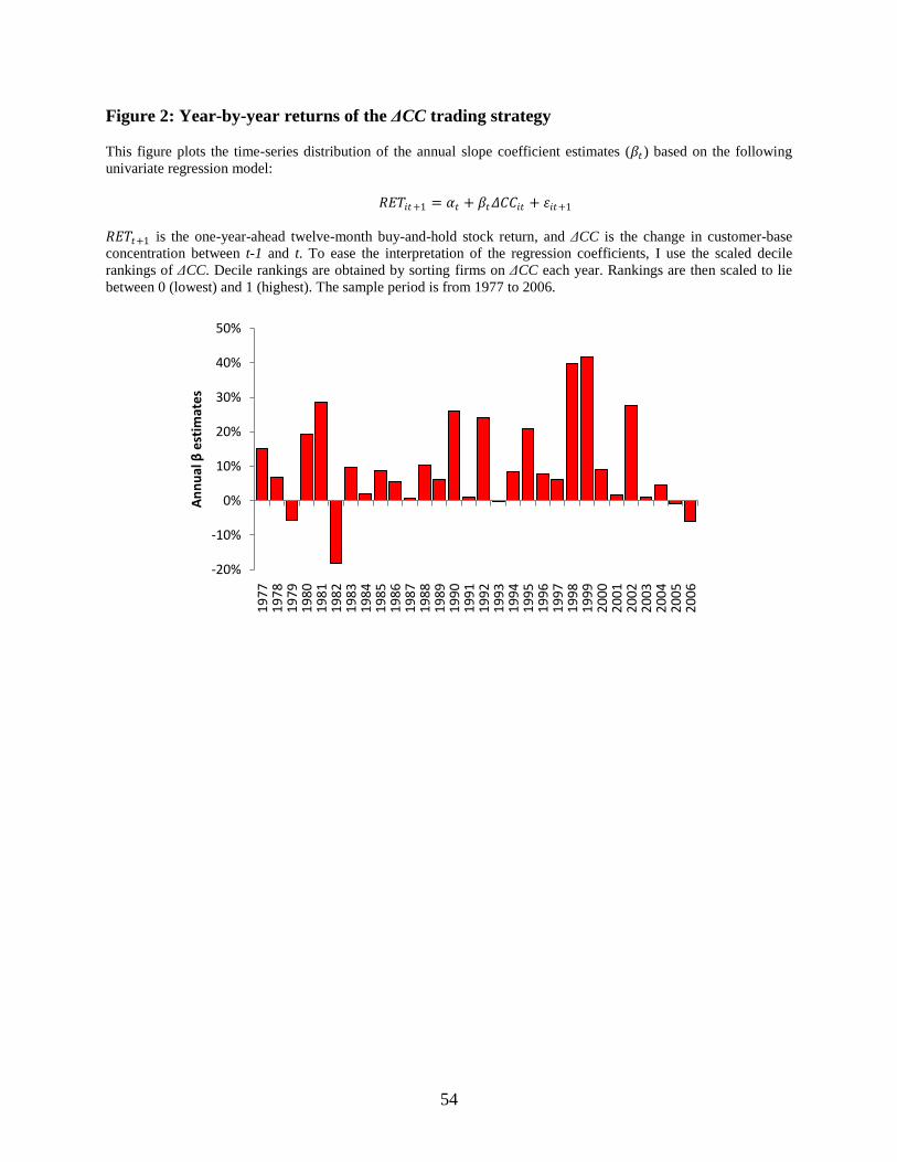
54
Figure 2: Year-by-year returns of the ΔCC trading strategy
This figure plots the time-series distribution of the annual slope coefficient estimates (𝛽𝑡) based on the following
univariate regression model:
𝑅𝐸𝑇𝑖𝑡+1 = 𝛼𝑡 + 𝛽𝑡𝛥𝐶𝐶𝑖𝑡 + 휀𝑖𝑡+1
𝑅𝐸𝑇𝑡+1 is the one-year-ahead twelve-month buy-and-hold stock return, and ΔCC is the change in customer-base
concentration between t-1 and t. To ease the interpretation of the regression coefficients, I use the scaled decile
rankings of ΔCC. Decile rankings are obtained by sorting firms on ΔCC each year. Rankings are then scaled to lie
between 0 (lowest) and 1 (highest). The sample period is from 1977 to 2006.
-20%
-10%
0%
10%
20%
30%
40%
50%
19
77
19
78
19
79
19
80
19
81
19
82
19
83
19
84
19
85
19
86
19
87
19
88
19
89
19
90
19
91
19
92
19
93
19
94
19
95
19
96
19
97
19
98
19
99
20
00
20
01
20
02
20
03
20
04
20
05
20
06
An
nu
al β
est
imat
es

55
References
Amihud, Y., 2002. Illiquidity and stock returns: Cross-section and time-series effects. Journal of
Financial Markets 5, 31-56.
Amir, E., and B. Lev, 1996. Value-relevance of non-financial information: The wireless
communication industry. Journal of Accounting and Economics 22, 3-30.
Anderson, S. W., 2007. Managing costs and cost structure throughout the value chain: Research
on strategic cost management. In C. S. Chapman, A. G. Hopwood, and M. D. Shields (Eds.).
Handbook of Management Accounting Research Volume 2, 481-506. Amsterdam, The
Netherlands: Elsevier.
Balakrishnan, R., T. Linsmeier, and M. Venkatachalam, 1996. Financial benefits from JIT
adoption: Effects of customer concentration and cost structure. The Accounting Review 71,
183-205.
Ball, R., and E. Bartov, 1996. How naïve is the stock market‟s use of earnings information?
Journal of Accounting and Economics 21, 319-337.
Ball, R., and P. Brown, 1968. An empirical evaluation of accounting numbers. Journal of
Accounting Research 6, 159-177.
Banz, R., 1981. The relationship between return and market value of common stocks. Journal of
Financial Economics 9, 3-18.
Basu, S., 1997. The conservatism principle and the asymmetric timeliness of earnings. Journal of
Accounting and Economics 24, 3-37.
Beaver, W., 1970. The time-series behavior of earnings. Journal of Accounting Research 8, 319-
346.
Bernard, V. L., and J. K. Thomas, 1989. Post-earnings announcement drift: Delayed price
response or risk premium? Journal of Accounting Research 27, 1-36.
Bernard, V. L., and J. K. Thomas, 1990. Evidence that stock prices do not fully reflect the
implications of current earnings for future earnings. Journal of Accounting and Economics
13, 305-340.
Bernard, V. L., J. K. Thomas, and J. Wahlen, 1997. Accounting-based stock price anomalies:
Separating market inefficiencies from risk. Contemporary Accounting Research 14, 89-136.
Bloomfield, R., 2002. The incomplete revelation hypothesis and financial reporting. Accounting
Horizons 16, 233–243.
Burke, G. J., J. E. Carrillo, and A. J. Vakharia, 2007. Single versus multiple supplier sourcing
strategies. European Journal of Operations Research 182, 95-112.
Cohen, L., and A. Frazzini, 2008. Economic links and predictable returns. Journal of Finance 63,
1977-2011.
Cowley, P. R., 1988. Market Structure and Business Performance: An Evaluation of Buyer/Seller
Power in the PIMS Database. Strategic Management Journal 9, 271-278
Daniel, K., and S. Titman, 2006. Market reactions to tangible and intangible information. Journal
of Finance 61, 1605-1643.
Dhar, R., and R. Glazer, 2003. Hedging customers. Harvard Business Review 81 (May), 86–92.
Dichev, I. D., 1998. Is the risk of bankruptcy a systematic risk? Journal of Finance 53, 1131-
1147.
Ertimur, Y., J. Livnat, and M. Martikainen, 2003. Differential market reactions to revenue and
expense surprises. Review of Accounting Studies 8, 185-211.

56
Fairfield, P., and T. Yohn, 2001. Using asset turnover and profit margin to forecast changes in
profitability. Review of Accounting Studies 6, 371-385.
Fama, E., 1998. Market efficiency, long-term returns, and behavioral finance. Journal of
Financial Economics 49, 283-306.
Fama, E., and K. French, 1993. Common risk factors in the return on bonds and stocks. Journal
of Financial Economics 33, 3-56.
Fama, E., and J. MacBeth, 1973. Risk, return and equilibrium: Empirical tests. Journal of
Political Economy 81, 607-639.
Financial Accounting Standards Board, 1976. Statement of Financial Accounting Standards
No.14: Financial Reporting for Segments of a Business Enterprise.
Financial Accounting Standards Board, 1979. Statement of Financial Accounting Standards No.
30: Disclosure of Information about Major Customers − an amendment of FASB Statement
No. 14.
Financial Accounting Standards Board, 1997. Statement of Financial Accounting Standards No.
131: Disclosures about Segments of an Enterprise and Related Information.
Francis, J., and K. Schipper, 1999. Have financial statements lost their relevance? Journal of
Accounting Research 37, 319-352.
Freeman, R., J. Ohlson, and S. Penman, 1982. Book rate-of-return and prediction of earnings
changes: An empirical investigation. Journal of Accounting Research 20, 3-42.
Galbraith, C. S., and C. H. Stiles, 1983. Firm profitability and relative firm power. Strategic
Management Journal 4, 237-249.
Galbraith, J. K., 1952. American capitalism: The concept of countervailing power. Boston, MA:
Houghton Mifflin.
Gebhardt, W. R., C. M. C. Lee, and B. Swaminathan, 2001. Toward an implied cost of capital.
Journal of Accounting Research 39, 135-176.
Gosman, M., T. Kelly, P. Olsson, and T. Warfield, 2004. The profitability and pricing of major
customers. Review of Accounting Studies 9, 117-139.
Granger, C. W. J., 1969. Investigating causal relations by econometric models and cross-spectral
methods. Econometrica 37, 424-428.
Griffin, J. M., and M. L. Lemmon, 2002. Book-to-market equity, distress risk and stock returns.
Journal of Finance 57, 2317-2336.
Gupta, S., D. R. Lehmann, and J. A. Stuart, 2004. Valuing customers. Journal of Marketing
Research 41, 7-18.
Hong, H., T. Lim, and J. Stein, 2000. Bad news travels slowly: Size, analyst coverage, and the
profitability of momentum strategies. Journal of Finance 55, 265-295.
Hou, K., and D. T. Robinson, 2006. Industry concentration and average stock returns. Journal of
Finance 61, 1927-1956.
Jackson, B., 1985. Winning and keeping industrial customers: The dynamics of customer
relationships. Lexington, MA: Lexington Books.
Kalwani, M. U., and N. Narayandas, 1995. Long-term manufacturer-supplier relationships: Do
they pay off for supplier firms? Journal of Marketing 59, 1-16.
Kelly, T., and M. Gosman, 2000. Increased buyer concentration and its effects on profitability in
the manufacturing sector. Review of Industrial Organization 17, 41-59.
Kinney, M. R., and W. F. Wempe, 2002. Further evidence on the extent and origins of JIT‟s
profitability effects. The Accounting Review 77, 203-225.

57
Kraljic, P., 1983. Purchasing must become supply management. Harvard Business Review 61
(September), 109-117.
Kumar, N., 1996. The power of trust in manufacturer-retailer relationships. Harvard Business
Review 74 (November), 92-106.
LaFrance, V. A., 1979. The impact of buyer concentration: An extension. Review of Economics
and Statistics 61, 475-476.
Lee, H., V. Padmanabhan, and S. Whang, 1997. Information distortion in a supply chain: The
bullwhip effect. Management Science 43, 546–558.
Lev, B., 2001. Intangibles: Management, measurement, and reporting. Washington, D.C.:
Brookings Institution Press.
Lustgarten, S., 1975. The impact of buyer concentration in manufacturing industries. Review of
Economics and Statistics 57, 125-132.
Matsumura, E. L., and J. D. Schloetzer, 2009. Strong buyers and inter-organizational cost
management. Working paper.
Menzly, L., and O. Ozbas, 2006. Cross-industry momentum. Working paper.
Nagel, S., 2005. Short sales, institutional investors and the cross-section of stock returns. Journal
of Financial Economics 78, 277-309.
Newey, W., and K. West, 1987. A simple, positive, semi-definite, heteroskedasticity and
autocorrelation consistent covariance matrix. Econometrica 55, 703-708.
Newmark, C. M., 1989. Administrative control, buyer concentration, and price-cost margins.
Review of Economics and Statistics 71, 74-79.
Niraj, R., M. Gupta, and C. Narasimhan, 2001. Customer profitability in a supply chain. Journal
of Marketing 65, 1-16.
Nissim, D., and S. H. Penman, 2001. Ratio analysis and equity valuation: From research to
practice. Review of Accounting Studies 6, 109-154.
Ohlson, J., 1980. Financial ratios and the probabilistic prediction of bankruptcy. Journal of
Accounting Research 18, 109-131.
Palepu, K. G., P. M. Healy, and V. L. Bernard, 2004. Business analysis and valuation using
financial statements. Thomson Learning, 3rd Edition.
Panayides, P. M., and Y. H. Venus Lun, 2009. The impact of trust on innovativeness and supply
chain performance. International Journal of Production Economics 122, 35-46.
PBS Frontline, 2004. Is Wal-Mart good for America? PBS Frontline Online. Available at:
http://www.pbs.org/wgbh/pages/frontline/shows/walmart/.
Porter, M. E., 1974. Consumer behavior, retailer power and market performance in consumer
goods industries. Review of Economics and Statistics 56, 419–436.
Ravenscraft, D., 1983. Structure-profit relationships at the line of business and industry level.
Review of Economics and Statistics 65, 22-31.
Scherer, F. M., 1970. Industrial market structure and economic performance. Chicago, IL: Rand
McNally.
Sloan, R., 1996. Do stock prices fully reflect information in accruals and cash flows about future
earnings? The Accounting Review 71, 289-315.
Soliman, M. T., 2008. The use of DuPont analysis by market participants. The Accounting
Review 83, 823-854.
Statman, M., 1987. How many stocks make a diversified portfolio? Journal of Financial and
Quantitative Analysis 22, 353-363.

58
Stattman, D., 1980. Book values and stock returns. The Chicago MBA: A Journal of Selected
Papers 4, 25-45.
Sunder, S., 1973. Relationship between accounting changes and stock prices: Problems of
measurement and some empirical evidence. Journal of Accounting Research 11, 1-45.
Sunder, S., 1975. Stock price and risk related to accounting changes in inventory valuation. The
Accounting Review 50, 305-315.
Treleven, M., and S. B. Schweikhart, 1988. A risk/benefit analysis of sourcing strategies: single
vs. multiple sourcing. Journal of Operations Management 7, 93-114.
Zhang, X. F., 2006. Information uncertainty and stock returns. Journal of Finance 61, 105-137.