custom device for low-dose gamma irradiation of...
TRANSCRIPT
CUSTOM DEVICE FOR LOW-DOSE GAMMA IRRADIATION OF
BIOLOGICAL SAMPLES
A Thesis
by
RUOMING BI
Submitted to the Office of Graduate Studies of Texas A&M University
in partial fulfillment of the requirements for the degree of
MASTER OF SCIENCE
December 2011
Major Subject: Health Physics
CUSTOM DEVICE FOR LOW-DOSE GAMMA IRRADIATION OF
BIOLOGICAL SAMPLES
A Thesis
by
RUOMING BI
Submitted to the Office of Graduate Studies of Texas A&M University
in partial fulfillment of the requirements for the degree of
MASTER OF SCIENCE
Approved by:
Chair of Committee, John R. Ford Committee Members, John W. Poston, Sr. Michael A. Walker Head of Department, Raymond J. Juzaitis
December 2011
Major Subject: Health Physics

iii
ABSTRACT
Custom Device for Low-Dose Gamma Irradiation of Biological Samples.
(December 2011)
Ruoming Bi, B.S., Texas A&M University
Chair of Advisory Committee: Dr. John Ford
When astronauts travel in space, their primary health hazards are high-energy
cosmic radiations from galactic cosmic rays (GCR). Most galactic cosmic rays have
energies between 100 MeV and 10 GeV. For occupants inside of a space shuttle, the
structural material is efficient to absorb most of the cosmic-ray energy and reduce the
interior dose rate to below 1.2 mGy per day. However, the biological effects of
prolonged exposure to low-dose radiation are not well understood. The purpose of this
research was to examine the feasibility of constructing a low-dose irradiation facility to
simulate the uniform radiation field that exists in space. In this research, we used a pre-
manufactured incubator, specifically the Thermo Scientific Forma Series II Water
Jacketed CO2 Incubator, to act as shielding and simulate the exterior of the space shuttle.
To achieve the desired dose rate (< 1 mGy/h) inside the incubator volume, the computer
code MCNPX was used to determine required source activity and distance between the
shielding and source. Once the activity and distance were calculated, an experiment was
carried out to confirm the simulation results, which used survey meters and
thermoluminescence dosimeters (TLDs) to map the radiation field within the incubator.

iv
Based on results from the MCNPX simulation and the actual experiment, a uniform
radiation field was achieved in the rear space of the incubator, which accounted for the
majority of the incubator volume. Furthermore, the actual dose rate had a range from
0.298 to 0.696 mGy/h, hence meeting the initial design criteria.

v
ACKNOWLEDGEMENTS
This research was supported by the Center for Bio-nanotechnology and
Environmental Research at Texas Southern University as part of a NASA research grant.
I would like to thank my committee chair, Dr. John Ford, and my committee
members, Dr. John Poston and Dr. Michael Walker, for their guidance and support
throughout the course of this research. I would also like to thank all the people of the
Nuclear Science Center at Texas A&M University, particularly Dr. Warren Reece and
Dr. Latha Vansudevan, for their efforts assisting me to complete this research. I would
like to thank all my friends, especially Fada Guan for giving me valuable MCNP
support, and Shaoyong Feng for proofreading. Finally, I thank my family members for
their love and encouragement.

vi
NOMENCLATURE
GCR Galactic Cosmic Ray
LET Linear Energy Transfer
RBE Relative Biological Effectiveness
MCNP Monte Carlo N-Particle
MCNPX Monte Carlo N-Particle eXtension
TLD Thermoluminescence Dosimeters
HVL1 First Half-Value Layers
HVL2 Second Half-Value Layers
HC Homogeneity Coefficient
hνeq Equivalent Photon Energy

vii
TABLE OF CONTENTS
Page
ABSTRACT .......................................................................................................... iii
ACKNOWLEDGEMENTS ................................................................................... v
NOMENCLATURE .............................................................................................. vi
TABLE OF CONTENTS....................................................................................... vii
LIST OF FIGURES ............................................................................................... ix
LIST OF TABLES................................................................................................. xii
I INTRODUCTION...................................................................................... 1
I. A Cosmic Rays............. .................................................................... 1 I. B Radiation Dose for Astronauts....................................................... 2 I. C Previous Designs of Low Dose Rate Irradiation Facilities.............. 4 I. D Thermoluminescence Detector (TLD)............. .............................. 9 I. E TLD Reader .................................................................................. 10 I. F Gamma Interactions in Matter........................................................ 11 I. G X-Ray Beam Quality Specification ............................................... 12 I. H Relative Error ............................................................................... 13
II MODELS AND METHODS ...................................................................... 14
II. A Overall Design............................................................................. 14 II. B Source.......................................................................................... 16 II. C Shielding...................................................................................... 20 II. D Distance....................................................................................... 23
III MEASUREMENTS AND SIMULATION.................................................. 25 III. A TLD ........................................................................................... 25
III. B MCNPX Simulation........... ........................................................ 37
IV DISCUSSION ............................................................................................ 54
viii
Page
V CONCLUSION AND FUTURE WORK ................................................... 58 V.A Conclusion .................................................................................. 58 V.B Future work........ ......................................................................... 58
REFERENCES ...................................................................................................... 60
APPENDIX A ....................................................................................................... 62
APPENDIX B........................................................................................................ 65
APPENDIX C........................................................................................................ 66
APPENDIX D ....................................................................................................... 67
APPENDIX E........................................................................................................ 70
APPENDIX F ........................................................................................................ 76
VITA..................................................................................................................... 82
ix
LIST OF FIGURES
FIGURE Page
I.1 Primary cosmic ray energy spectrum (Mishev et al. 2004). ...................... 2 I.2 Schematic of irradiator system constructed by University of Medicine and
Dentistry of New Jersey-New Jersey Medical School (Howell et al. 1997) 6 I.3 Schematic of experiment conducted by Sakai et al. 2003. ........................ 7 I.4 Typical low dose irradiation facility, Tokyo, Japan (Sakai et al. 2003)..... 7 I.5 MIT liquid source irradiator (Olipitz et al. 2010). .................................... 8 I.6 Schematic of a basic TLD reader ............................................................. 10 I.7 Relative importance of the three common gamma interaction types ......... 11 II.1 Top view of irradiation system ................................................................ 15 II.2 Photo of the actual experiment setup ....................................................... 15 II.3 Co-60 neutron activation schematic ......................................................... 17 II.4 The activity of an activator detector with respect to time ......................... 20 II.5 Thermo Scientific Forma Series II Water Jacketed CO2 Incubator ........... 21 II.6 Simplified incubator diagram with bacteria culture vessel........................ 23 III.1 TLD locations within the incubator.......................................................... 25 III.2 Equivalent photon energy vs. HVL1 in copper or aluminum (Attix 2004) 27 III.3 Thermoluminescent response of LiF for photon energy from 6 to 2800 keV (Attix 2004)............................................................................. 28 III.4 Glow curve of TLD #1 after exposure to 0.786 R X-ray .......................... 30 III.5 Glow curve of TLD #3 after exposure to 0.786 R X-ray .......................... 31
x
FIGURE Page
III.6 Glow curve of TLD #4 after exposed to 0.786 R X-ray............................ 31 III.7 XY cross section of the irradiation system ............................................... 38 III.8 XZ cross section of the irradiation system ............................................... 38 III.9 XY cross section of the irradiation system with photon paths................... 39 III.10 XZ cross section of the irradiation system with photon paths .................. 39 III.11 Gamma fluence distribution in Plane A .................................................. 42 III.12 Gamma fluence distribution in Plane B................................................... 42 III.13 Gamma fluence distribution in Plane C................................................... 43 III.14 Gamma fluence distribution in Plane D .................................................. 43 III.15 Gamma fluence distribution in Plane E ................................................... 44 III.16 Gamma fluence distribution in Plane F ................................................... 44 III.17 Gamma fluence distribution in Plane G .................................................. 45 III.18 Distribution of averaged absorbed dose from single source photon in Plane A................................................................................................... 48 III.19 Distribution of averaged absorbed dose from single source photon in Plane B ................................................................................................. 49 III.20 Distribution of averaged absorbed dose from single source photon in Plane C................................................................................................... 49 III.21 Distribution of averaged absorbed dose from single source photon in Plane D................................................................................................... 50 III.22 Distribution of averaged absorbed dose from single source photon in Plane E ................................................................................................... 50 III.23 Distribution of averaged absorbed dose from single source photon in Plane F ................................................................................................... 51

xi
FIGURE Page
III.24 Distribution of averaged absorbed dose from single source photon in Plane G................................................................................................... 51
xii
LIST OF TABLES
TABLE Page I.1 Recorded dose rate of recent NASA space programs ............................... 4 II.1 Neutron activation parameters for several materials ................................. 18 II.2 Specifications of Thermo Scientific Forma Series II Water Jacketed CO2 Incubator ................................................................................................. 22 III.1 Calibration filtration metal thicknesses and exposures ............................. 26
III.2 TLD calibration results after exposure to 0.786 and 1.086 R x-ray with equivalent photon energy of 160 keV ...................................................... 29
III.3 Modified TLD calibration results............................................................. 32
III.4 Results of seven different exposures measured in nanocoulombs (nC) ..... 33
III.5 Results of seven different exposures measured in roentgens (R) .............. 34
III.6 Absorbed dose of seven TLD exposures .................................................. 35
III.7 Summary of reactor operations from 6/14/10 to 7/12/10 .......................... 36
III.8 Corrected absorbed dose of seven TLD exposures ................................... 37
III.9 Conversion coefficients for air kerma per unit fluence (Ka/ φa) for monoenergetic photons........................................................................... 47
III.10 MCNPX simulation of averaged absorbed dose from single source photon at various locations ...................................................................... 52 III.11 Comparison of MCNPX simulation and measured results of total absorbed dose in eight hours................................................................................... 53 IV.1 Comparison of total absorbed dose between frontal and rear TLDs for the actual experiment and simulation............................................................. 55

1
I. INTRODUCTION
I.A Cosmic Rays
Cosmic rays may broadly be divided into two categories: primary cosmic rays
and secondary cosmic rays. Primary cosmic rays are energetic particles from extra-
terrestrial origin that constantly bombard earth's atmosphere. They consist of about 90%
high-energy protons, 9% helium and other heavier nuclei and a small percentage of
electron and gamma rays (Becker, et al. 2007). As they propagate, primary cosmic rays
can interact with interstellar medium to generate secondary cosmic rays. The ratio of
secondary/primary nuclei is highly dependent upon the primary nuclei energy (E).
According to NASA, the ratio of secondary to primary nuclei is observed to decrease
approximately as E-0.5 with increasing energy (Simpson 1983).
Like other ionizing radiation, cosmic rays, especially galactic cosmic rays
(GCR), pose a significant health risk for astronauts on interplanetary missions due to
their energetic nature. GCR have a wide range of energies, usually from 109 eV (1 GeV)
to 1020 eV (108 TeV). For comparison, the most powerful man-made particle
accelerators currently can only produce 1013 eV. The number of cosmic rays with
energies beyond 1 GeV decreases by about a factor of 50 for every factor of 10 increase
in energy (Mishev et al. 2004). The primary cosmic ray spectrum is shown in Figure I.1.
____________ This thesis follows the style of Health Physics.

2
Figure I.1. Primary cosmic ray energy spectrum (Mishev et al. 2004).
I.B Radiation Dose for Astronauts
The absorbed dose (D) is defined as the amount of energy deposited in bulk
material, which is commonly expressed as the product of particles fluence (F) and linear
energy transfer (L) as shown in Equation 1.
LFD * (1)

3
Relative biological effectiveness (RBE) is used to relate the risks of different
particles to the human body, which is defined as the ratio of the dose of gamma rays to the
radiation under study that will produce an equal level of effect. To represent the knowledge
of RBE, radiation weighting factors (WR) were assigned to different kind of radiations. As
shown in Equation 2, dose equivalent (H) is defined as the product of absorbed dose and
radiation weighting factor.
RWDH * (2)
To evaluate the organ dose or organ dose equivalent, the dose or dose equivalent
are summed over the LET spectra at the tissue of interest.
The amount of radiation dose received by astronauts depends on orbital
inclination, altitude, position in the solar cycle and mission duration (Cucinotta 2010).
Nevertheless, absorbed doses or dose rates were recorded by dosimetry badges worn by
astronauts for each NASA space mission. A summary of recent NASA space programs
and their corresponding doses is shown in Table I.1.

4
Table I.1. Recorded dose rate of recent NASA space programs (Cucinotta 2010)
I.C Previous Designs of Low Dose Rate Irradiation Facilities
Although the linear non-threshold model is a widely accepted hypothesis in
current radiation protection practices, the biological effects of prolonged exposure due to
low-dose radiation are not well understood. According to the National Radiological
Protection Board (NRPB), the terms of "low dose" and "low dose rate" are defined as
below 100 mGy and below 5 mGy per hour (Wakeford and Tawn 2010).
As early as the 1970s, health physicists attempted to study the effects of ionizing
radiation on plants and animals under natural conditions by constructing several large
scale outdoor irradiators. Amongst the many, two facilities located in Canada were the

5
most noticeable due to their size and irradiation duration. The Field Irradiator - Gamma
(FIG) was designed to monitor the effects of a fixed gradient of gamma radiation on a
boreal forest. It was used for 14 years to study plant community ecology. Its animal
counterpart, the zoological environment under stress (ZEUS) facility, was used for 4
years to study small mammal health and population (Mihok 2004). Ecological results
from such large scale field experiment provided valuable data to develop a practical
system for environmental protection (ICRP 2003). However, large outdoor irradiators
faced statistical and methodological difficulties when smaller sample sizes were selected
for more in-depth studies. For this reason, more modern studies favor smaller indoor
facilities.
Several experiments were conducted in 2008 at Chalk River Laboratories,
Canada, to simulate potential occupational exposure by exposing mice to chronic low-
dose gamma radiation. In such experiments, unrestrained mice in their plastic cages were
irradiated with a Co-60 open beam source (GammaBeam 150, Atomic Energy of Canada
Limited). Animals were exposed daily to about 0.33 mGy of gamma radiation delivered
at low dose rate (0.7 mGy/h), and the exposure was repeated 5 days per week for a
duration up to 90 weeks. Activity lost to decay over this extended period was
compensated by regularly adjusting the distance between the source and the animals to
maintain the stated daily dose and dose rate (Mitchel et al. 2008).
Using the same principle of dose-to-distant relationship, more advanced
irradiator prototypes were built. One of the prototypes was constructed at the New Jersey
Medical School, which coupled a computer controlled variable mercury attenuator with

6
a cesium-137 irradiator. The operator could control the target dose rate by introducing a
layer of mercury between source and cages from the mercury attenuator while keeping
source activity constant. This system could accommodate six cages placed at different
distances from the source, hence, achieving different target dose rates. A schematic of
this irradiator system is shown in Figure I.2.
Figure I.2. Schematic of irradiator system constructed by University of Medicine and Dentistry of New Jersey-New Jersey Medical School (Howell et al. 1997).
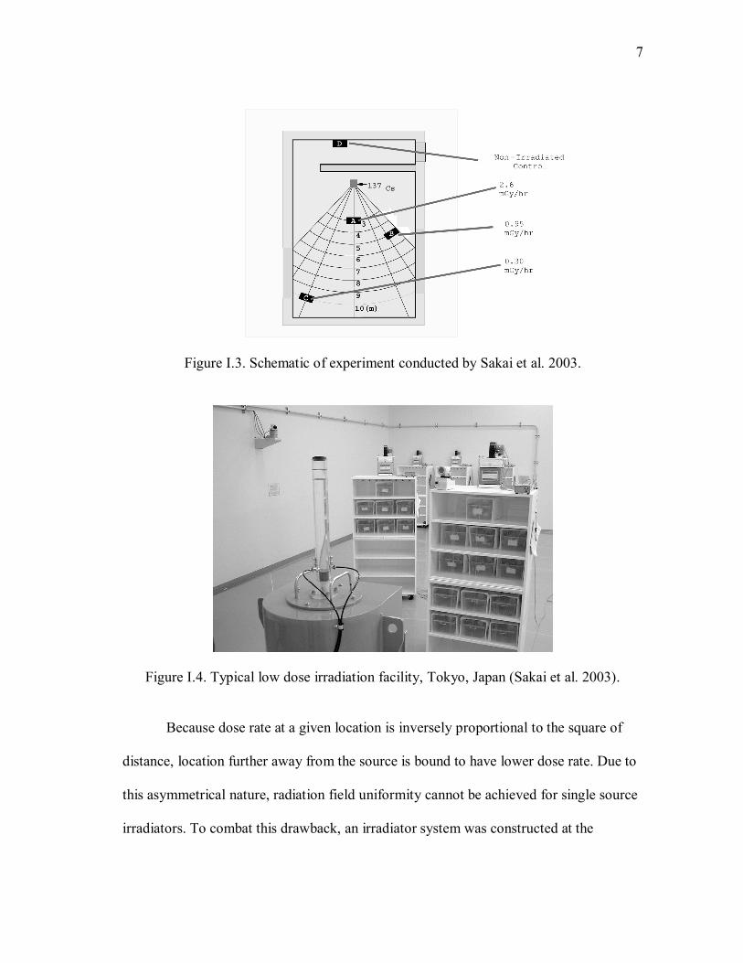
South Korea (Shin et al. 2010) and Japan (Ishida et al. 2010) have also conducted
comparable research experiments to study the effect of low-dose radiation by converting
the entire room into an irradiation chamber. As shown in Figure I.3 and I.4, the
experiments use distance as the sole means to modify dose rate by placing test subjects
at defined distances from a single source (Sakai et al. 2003).
7
Figure I.3. Schematic of experiment conducted by Sakai et al. 2003.
Figure I.4. Typical low dose irradiation facility, Tokyo, Japan (Sakai et al. 2003).
Because dose rate at a given location is inversely proportional to the square of
distance, location further away from the source is bound to have lower dose rate. Due to
this asymmetrical nature, radiation field uniformity cannot be achieved for single source
irradiators. To combat this drawback, an irradiator system was constructed at the

8
Massachusetts Institute of Technology (MIT), which used liquid radioactive source. The
liquid was made by mixing varying activities of I-125 into a sodium hydroxide (NaOH)
solution to maintain the desired dose rate. Shown in Figure I.5, the irradiator consisted a
plastic cart (PC) holding an aluminum tray (T) and a flood phantom (P). The phantom
was filled with radioactive liquid and served as radiation source. A steel cart (SC)
holding the cages fits exactly above the plastic cart. A leaded acrylic sheet (A) was
mounted on the steel cart to ensure radiation protection for experimenters (Olipitz 2010).
Figure I.5. MIT liquid source irradiator (Olipitz et al. 2010).
The MIT irradiator design was an advancement over one-source irradiator
designs, however, it did not entirely solve the problem because dose rates at higher
altitudes were still lower than the base, where the source was located. For this reason, it
9
is necessary to examine the feasibility of constructing a uniform low-dose irradiation
facility for the future experiments.
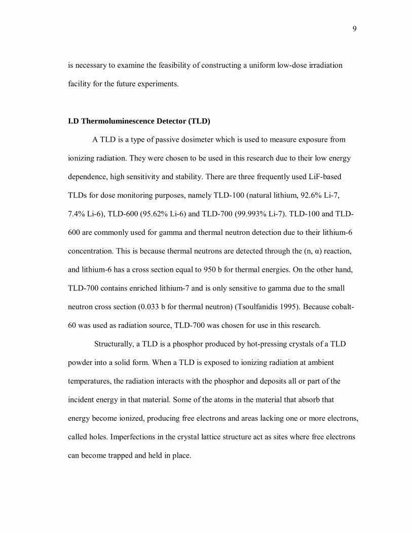
I.D Thermoluminescence Detector (TLD)
A TLD is a type of passive dosimeter which is used to measure exposure from
ionizing radiation. They were chosen to be used in this research due to their low energy
dependence, high sensitivity and stability. There are three frequently used LiF-based
TLDs for dose monitoring purposes, namely TLD-100 (natural lithium, 92.6% Li-7,
7.4% Li-6), TLD-600 (95.62% Li-6) and TLD-700 (99.993% Li-7). TLD-100 and TLD-
600 are commonly used for gamma and thermal neutron detection due to their lithium-6
concentration. This is because thermal neutrons are detected through the (n, α) reaction,
and lithium-6 has a cross section equal to 950 b for thermal energies. On the other hand,
TLD-700 contains enriched lithium-7 and is only sensitive to gamma due to the small
neutron cross section (0.033 b for thermal neutron) (Tsoulfanidis 1995). Because cobalt-
60 was used as radiation source, TLD-700 was chosen for use in this research.
Structurally, a TLD is a phosphor produced by hot-pressing crystals of a TLD
powder into a solid form. When a TLD is exposed to ionizing radiation at ambient
temperatures, the radiation interacts with the phosphor and deposits all or part of the
incident energy in that material. Some of the atoms in the material that absorb that
energy become ionized, producing free electrons and areas lacking one or more electrons,
called holes. Imperfections in the crystal lattice structure act as sites where free electrons
can become trapped and held in place.
10
To read the TLD chip, heating is required. Heating the crystal causes the crystal
lattice to vibrate, releasing the trapped electrons in the process. Released electrons return
to the original ground state, releasing the captured energy from ionization as light, hence
the name thermoluminescent. Released light is measured using a photomultiplier tube
and the number of photons counted is proportional to the quantity of radiation striking
the phosphor. In general, TLDs have a precision of approximately 15% for low doses.
This precision improves to approximately 3% for high doses (Berger and Hajek 2008).
I.E TLD Reader
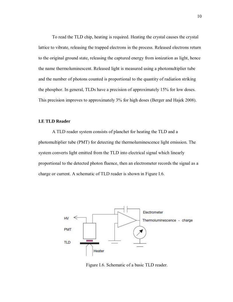
A TLD reader system consists of planchet for heating the TLD and a
photomultiplier tube (PMT) for detecting the thermoluminescence light emission. The
system converts light emitted from the TLD into electrical signal which linearly
proportional to the detected photon fluence, then an electrometer records the signal as a
charge or current. A schematic of TLD reader is shown in Figure I.6.
Figure I.6. Schematic of a basic TLD reader.

11
TLD glow curves can be generated from the TLD reader, which is the intensity
of emitted light in terms of charge or current plot against the crystal temperature or time.
The area under the curve is the total thermoluminescence signal emitted.
I.F Gamma Interactions in Matter
There are three common interactions when gamma photons interact with matter,
namely, the Compton Effect, Photoelectric Effect and Pair Production (Attix 2004). The
relative importance of the three interactions is summarized in Figure I.7, which
illustrates the regions in which each interaction is dominant.
Figure I.7. Relative importance of the three common gamma interaction types (Attix 2004).
The photoelectric effect is the process of ejection of an electron when an atom
absorbs energy from a gamma ray. The photon disappears in the process; some of its
12
energy overcomes the electron binding energy and the remainder is transferred to the
freed electron as kinetic energy. The newly freed electron is called a photoelectron.
The Compton Effect is a form of inelastic scattering, in which a gamma ray
interacts with a free or weakly bound electron and transfers part of its energy to the
electron. The results of the Compton Effect include energy decrease of the gamma ray
and the ejection of the electron by the atom, where the newly freed electron has kinetic
energy essentially equal to the energy lost by the gamma ray. The Compton Effect is the
dominant interaction in this research.
Pair Production is the creation of an electron and a positron pair. A gamma ray
with an energy at least 1.022 MeV can create an electron-positron pair when it is under
the influence of the strong electromagnetic field in the vicinity of a nucleus. If the
gamma-ray energy exceeds 1.022 MeV, the excess energy is shared between the electron
and the positron as kinetic energy. Although the threshold for this interaction is 1.022
MeV, the interaction has a low probability for photons below about 4 MeV (Oldenberg
and Rasmussen 1996).
I.G X-Ray Beam Quality Specification
TLD chips must be annealed and calibrated before use. For TLD-700s, filtered x-
rays are commonly used for calibration. The quality of an X-ray is usually specified in
terms of its attenuation characteristics in a reference medium (commonly in Cu and Al)
(Attix 2004), such as first and second half-value layers (HVL1, HVL2), homogeneity
coefficient (HC) and equivalent photon energy (hνeq). HVL1 is defined as the thickness

13
required to reduce the X-ray exposure by half in narrow-beam geometry. HVL2 is the
thickness necessary to reduce it by half again under the same conditions. The ratio
HVL1/HVL2 is the homogeneity coefficient, which approaches unity as the spectrum is
narrowed by filtration to approach monochromaticity. Lastly, hνeq is defined as the
quantum energy of a monoenergetic beam having the same HVL1 as the beam being
specified.
I.H Relative Error
In statistics, relative error is generally expressed as a percentage to reflect how a
quantity varies from the actual value. To obtain the relative error for a set of numbers,
one must first identify the variance or the standard deviation of the set. Equation 3, 4 and
5 can used to derive variance, standard deviation and relative error, respectively.
22 )(*1
1 XxN
si
i (3)
2ss (4)
relative error Xs
(5)
where, s2 is sample variance, N is sample size, xi is the value of index i, X is mean, s is
standard deviation (Rice 1995).

14
II. MODELS AND METHODS
II.A. Overall Design
The basic components of the low-dose irradiator include source and shielding
materials. To achieve the desired dose rate in a given space, one can manipulate the
thickness of shielding, the distance between source and the target, the strength of the
source or any combination of the three. However, for practical viability, this research
chooses to use a pre-manufactured incubator, specifically, the Thermo Scientific Forma
Series II Water Jacketed CO2 Incubator, to act as shielding and simulate the space
shuttle’s exterior. Due to this design choice, one can only modify the two remaining
factors, namely, the distance and the source strength to attain the desired dose rate.
The diagram of the irradiation system and the actual experiment setup are shown
in Figure II.1 and II.2, respectively, where a bacteria culture vessel (target) is placed
inside the incubator (shielding), which is surrounded by three, unit-length cobalt-60
wires.

15
Figure II.1: Top view of irradiation system.
Figure II.2: Photo of the actual experiment setup.
16
II.B. Source
Radiation field strength directly depends on source activity. More specifically,
the activity of each cobalt wire is required to compute the dose rate within the target.
The cobalt wire of our choice (manufacturer Alfa Aesar, stock No. 10947, Lot No
B23R004) has an exact diameter (0.25 mm) and length (1 m). Such a geometry can be
used to calculate the volume of each wire using Equation 6,
hrV 2 (6)
where V, r, h refer to volume, radius, and height, respectively.
Once the wire volume is determined, its mass can be calculated using Equation 7,
Vm (7)
where, m is mass and ρ is density.
Consequently, the number of molecules can be calculated by using Equation 8,
Na
MmN
(8)
where, N is the number of molecules in the given mass, M is molar mass, and Na is
Avogadro's constant.
Finally, the activity of each wire can be calculated by using Equations 9 and 10,
2/1
)2ln(T
(9)
NA (10)
where, A refers to activity of a 100% pure cobalt-60 wire, λ refers to the decay constant
of Co-60, and T1/2 refers to its corresponding half life.

17
Complete calculation for the activity of each cobalt wire is shown in Appendix
C.
Once the possible maximum activity is calculated, one can choose an appropriate
activity lower than the maximum, which corresponds to the pre-determined target dose
rate. This was done by manipulating the Co-60 purity level using MCNPX simulation.
After the final Co-60 activity for each wire was determined, they were produced by
neutron activation in the reactor at the Nuclear Science Center. A schematic of the Co59
(n, γ) Co60 reaction is illustrated in figure II.3. Relevant neutron activation parameters
can be found in Table II.1.
Figure II.3. Co-60 neutron activation schematic.

18
Table II.1. Neutron activation parameters for several materials (Beckurts and Wirtz 1964)
.
In theory, the initial activity of each wire can be calculated using in Equation 11.
w
SmA *****0
(11)
where,
A0 = the activity of each wire at time of termination of neutron activation (t=0);
= neutron absorption cross section;
m = the mass of each wire in grams;
= Avogadro's constant, 6.023*1023 molecules/mole;
= neutron fluence rate, neutrons/cm2/s;
19
= fraction of target isotope in the sample, was 1 in this research, since Co59 is 100%
abundant;
S = saturation factor, 1-e-λt; and
w = the atomic weight of element.
However, in practice, the wires had to be compressed into coils and placed inside
aluminum capsules during activation, hence, one must account for the self-shielding and
attenuation effects. Additionally, neutron fluence rate around the cobalt wire coils could
not be guaranteed as constant for the entire activation duration.
Three wires were separately activated at reactor core position A4, using the
reactor in Nuclear Science Center of Texas A&M University. The initial activity of the
wires was estimated to be between 20 to 25 mCi. More detailed neutron activation
records from Nuclear Science Center are shown in Appendix D.
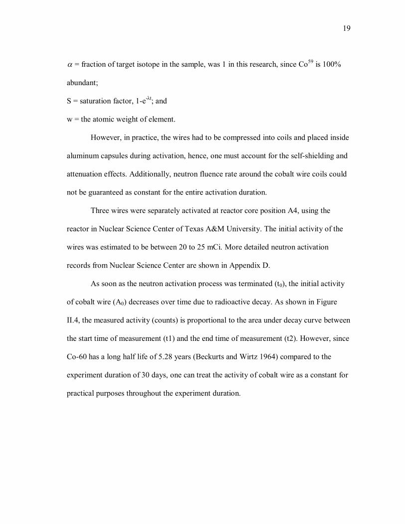
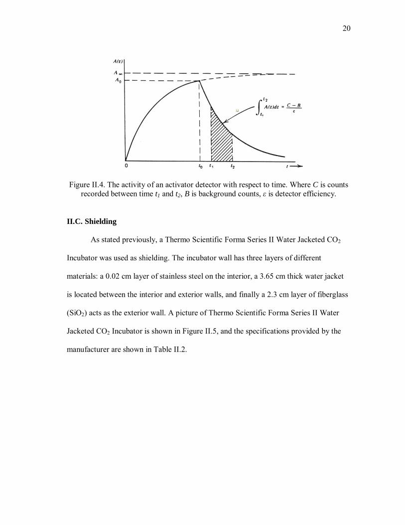
As soon as the neutron activation process was terminated (t0), the initial activity
of cobalt wire (A0) decreases over time due to radioactive decay. As shown in Figure
II.4, the measured activity (counts) is proportional to the area under decay curve between
the start time of measurement (t1) and the end time of measurement (t2). However, since
Co-60 has a long half life of 5.28 years (Beckurts and Wirtz 1964) compared to the
experiment duration of 30 days, one can treat the activity of cobalt wire as a constant for
practical purposes throughout the experiment duration.
20
Figure II.4. The activity of an activator detector with respect to time. Where C is counts recorded between time t1 and t2, B is background counts, ε is detector efficiency.
II.C. Shielding
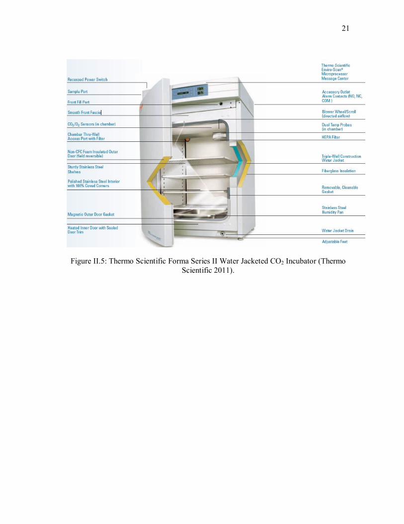
As stated previously, a Thermo Scientific Forma Series II Water Jacketed CO2
Incubator was used as shielding. The incubator wall has three layers of different
materials: a 0.02 cm layer of stainless steel on the interior, a 3.65 cm thick water jacket
is located between the interior and exterior walls, and finally a 2.3 cm layer of fiberglass
(SiO2) acts as the exterior wall. A picture of Thermo Scientific Forma Series II Water
Jacketed CO2 Incubator is shown in Figure II.5, and the specifications provided by the
manufacturer are shown in Table II.2.
21
Figure II.5: Thermo Scientific Forma Series II Water Jacketed CO2 Incubator (Thermo Scientific 2011).
22
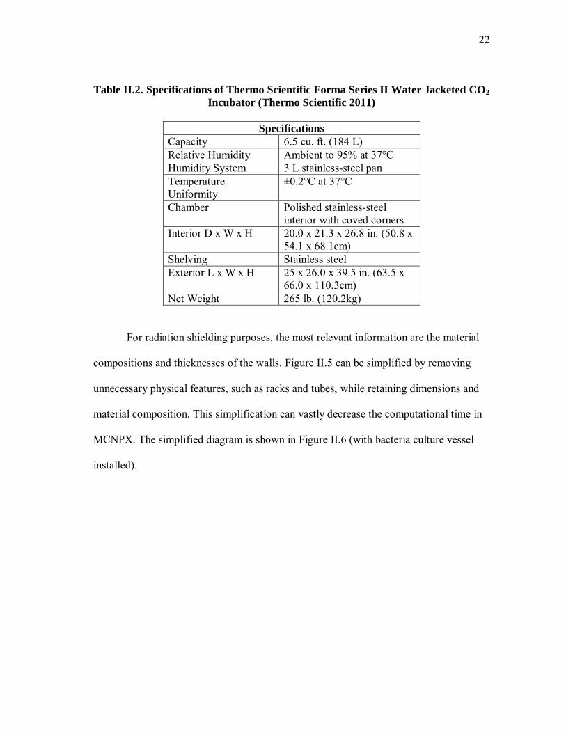
Table II.2. Specifications of Thermo Scientific Forma Series II Water Jacketed CO2 Incubator (Thermo Scientific 2011)
Specifications
Capacity 6.5 cu. ft. (184 L) Relative Humidity Ambient to 95% at 37°C Humidity System 3 L stainless-steel pan Temperature Uniformity
±0.2°C at 37°C
Chamber Polished stainless-steel interior with coved corners
Interior D x W x H 20.0 x 21.3 x 26.8 in. (50.8 x 54.1 x 68.1cm)
Shelving Stainless steel Exterior L x W x H 25 x 26.0 x 39.5 in. (63.5 x
66.0 x 110.3cm) Net Weight 265 lb. (120.2kg)
For radiation shielding purposes, the most relevant information are the material
compositions and thicknesses of the walls. Figure II.5 can be simplified by removing
unnecessary physical features, such as racks and tubes, while retaining dimensions and
material composition. This simplification can vastly decrease the computational time in
MCNPX. The simplified diagram is shown in Figure II.6 (with bacteria culture vessel
installed).

23
Figure II.6: Simplified incubator diagram with bacteria culture vessel.
II.D. Distance
Once the maximum source activity and the shielding materials are determined,
the distance required to achieve a required dose rate can be obtained using MCNPX. For
this research project, the method of choice is trial and error, also known as generate and
test. To do this, a randomly selected distance and source activity, calculated by methods
described in previous sections, along with shielding geometry are input into the MCNPX
code to generate the dose rate inside the forged bacteria culture vessel. Since the target
dose rate is inversely proportional to the square of the distance and proportional to
source activity, one must increase the distance or decrease source activity or a
combination of the two, if the calculated dose rate is higher than the planned dose rate,
or vice versa. The appropriate combinations of distance and source activity for the
planned bacterial vessel dose rate can be determined using methods described above. For

24
any given shielding geometry, there can be infinite numbers of distance and source
activity combinations. However, the laboratory room used to perform the experiment
could not accommodate distances greater than two meters. Due to this space constrain,
the most realistic combination was 1 meter distance and 23 mCi activity for each cobalt
wire. The geometry displayed in Figure II.6 was used in the MCNPX code that is found
in Appendix A.
25
III. MEASUREMENTS AND SIMULATION
III.A. TLD
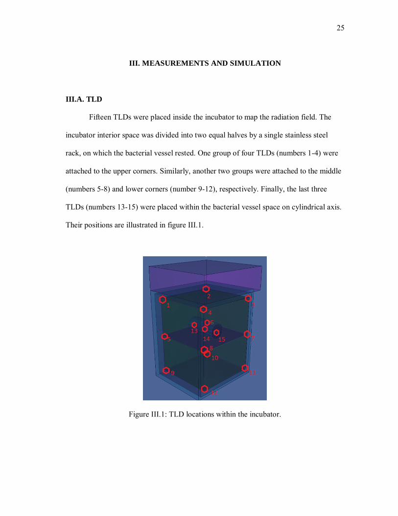
Fifteen TLDs were placed inside the incubator to map the radiation field. The
incubator interior space was divided into two equal halves by a single stainless steel
rack, on which the bacterial vessel rested. One group of four TLDs (numbers 1-4) were
attached to the upper corners. Similarly, another two groups were attached to the middle
(numbers 5-8) and lower corners (number 9-12), respectively. Finally, the last three
TLDs (numbers 13-15) were placed within the bacterial vessel space on cylindrical axis.
Their positions are illustrated in figure III.1.
Figure III.1: TLD locations within the incubator.
26
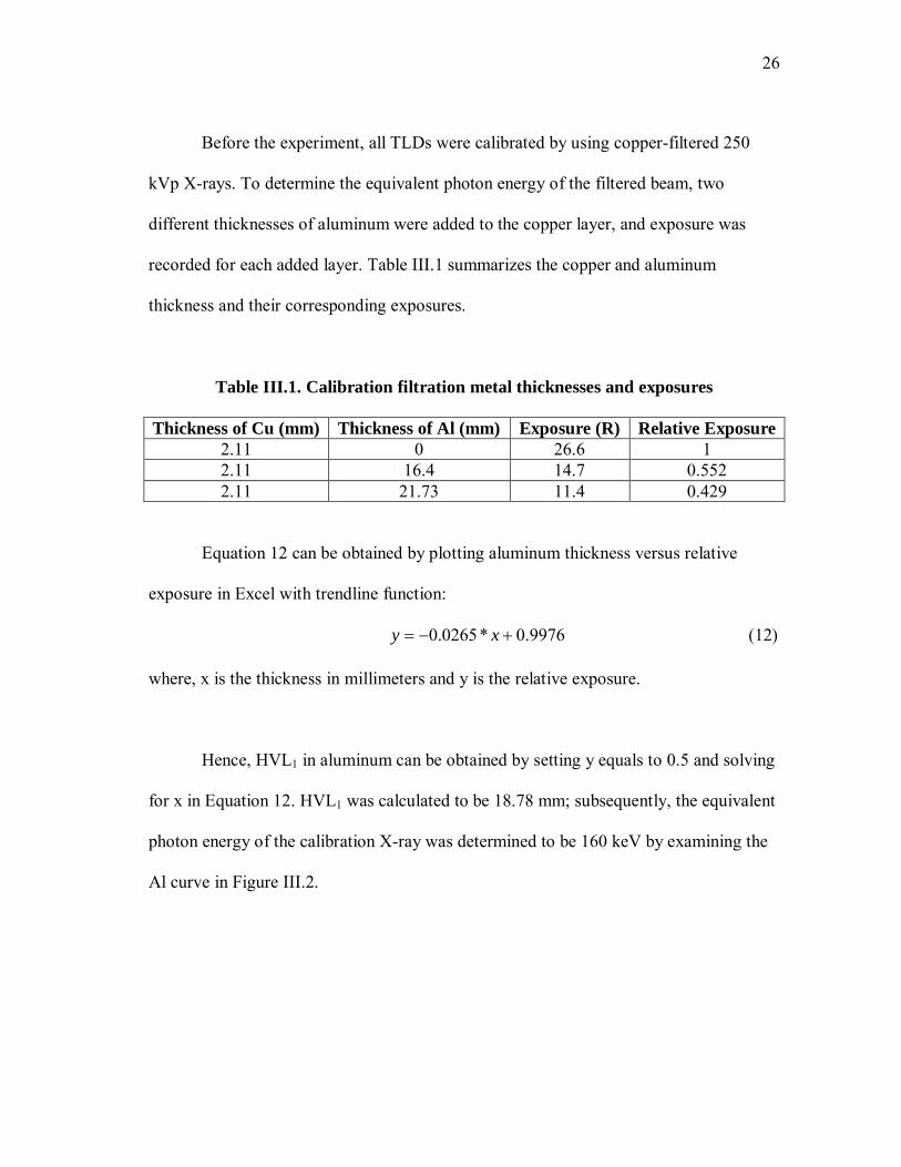
Before the experiment, all TLDs were calibrated by using copper-filtered 250
kVp X-rays. To determine the equivalent photon energy of the filtered beam, two
different thicknesses of aluminum were added to the copper layer, and exposure was
recorded for each added layer. Table III.1 summarizes the copper and aluminum
thickness and their corresponding exposures.
Table III.1. Calibration filtration metal thicknesses and exposures
Thickness of Cu (mm) Thickness of Al (mm) Exposure (R) Relative Exposure 2.11 0 26.6 1 2.11 16.4 14.7 0.552 2.11 21.73 11.4 0.429
Equation 12 can be obtained by plotting aluminum thickness versus relative
exposure in Excel with trendline function:
9976.0*0265.0 xy (12)
where, x is the thickness in millimeters and y is the relative exposure.
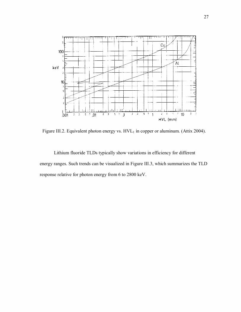
Hence, HVL1 in aluminum can be obtained by setting y equals to 0.5 and solving
for x in Equation 12. HVL1 was calculated to be 18.78 mm; subsequently, the equivalent
photon energy of the calibration X-ray was determined to be 160 keV by examining the
Al curve in Figure III.2.
27
Figure III.2. Equivalent photon energy vs. HVL1 in copper or aluminum. (Attix 2004).
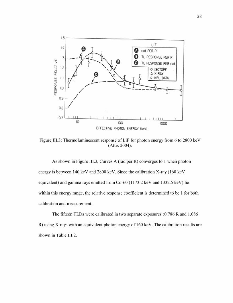
Lithium fluoride TLDs typically show variations in efficiency for different
energy ranges. Such trends can be visualized in Figure III.3, which summarizes the TLD
response relative for photon energy from 6 to 2800 keV.
28
Figure III.3: Thermoluminescent response of LiF for photon energy from 6 to 2800 keV (Attix 2004).
As shown in Figure III.3, Curves A (rad per R) converges to 1 when photon
energy is between 140 keV and 2800 keV. Since the calibration X-ray (160 keV
equivalent) and gamma rays emitted from Co-60 (1173.2 keV and 1332.5 keV) lie
within this energy range, the relative response coefficient is determined to be 1 for both
calibration and measurement.
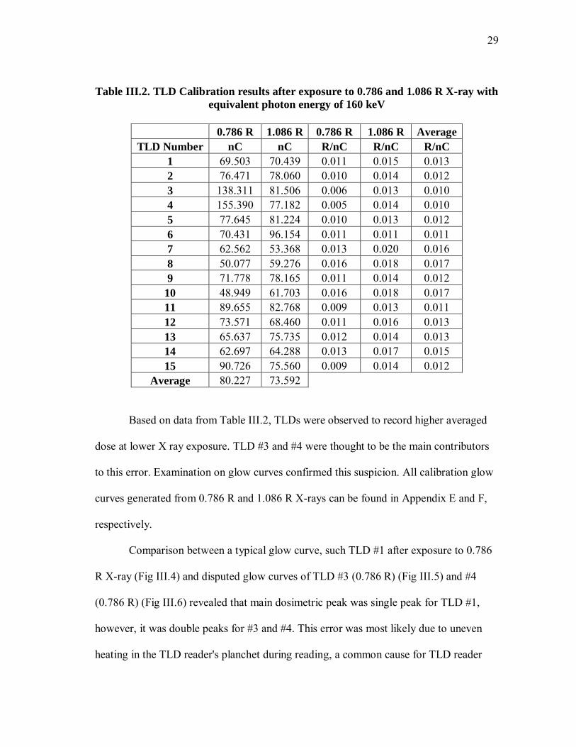
The fifteen TLDs were calibrated in two separate exposures (0.786 R and 1.086
R) using X-rays with an equivalent photon energy of 160 keV. The calibration results are
shown in Table III.2.
29
Table III.2. TLD Calibration results after exposure to 0.786 and 1.086 R X-ray with equivalent photon energy of 160 keV
0.786 R 1.086 R 0.786 R 1.086 R Average
TLD Number nC nC R/nC R/nC R/nC 1 69.503 70.439 0.011 0.015 0.013 2 76.471 78.060 0.010 0.014 0.012 3 138.311 81.506 0.006 0.013 0.010 4 155.390 77.182 0.005 0.014 0.010 5 77.645 81.224 0.010 0.013 0.012 6 70.431 96.154 0.011 0.011 0.011 7 62.562 53.368 0.013 0.020 0.016 8 50.077 59.276 0.016 0.018 0.017 9 71.778 78.165 0.011 0.014 0.012
10 48.949 61.703 0.016 0.018 0.017 11 89.655 82.768 0.009 0.013 0.011 12 73.571 68.460 0.011 0.016 0.013 13 65.637 75.735 0.012 0.014 0.013 14 62.697 64.288 0.013 0.017 0.015 15 90.726 75.560 0.009 0.014 0.012
Average 80.227 73.592
Based on data from Table III.2, TLDs were observed to record higher averaged
dose at lower X ray exposure. TLD #3 and #4 were thought to be the main contributors
to this error. Examination on glow curves confirmed this suspicion. All calibration glow
curves generated from 0.786 R and 1.086 R X-rays can be found in Appendix E and F,
respectively.
Comparison between a typical glow curve, such TLD #1 after exposure to 0.786
R X-ray (Fig III.4) and disputed glow curves of TLD #3 (0.786 R) (Fig III.5) and #4
(0.786 R) (Fig III.6) revealed that main dosimetric peak was single peak for TLD #1,
however, it was double peaks for #3 and #4. This error was most likely due to uneven
heating in the TLD reader's planchet during reading, a common cause for TLD reader

30
inaccuracy. Because thermoluminescence intensity emission is a function of the TLD
temperature (T), keeping the heating rate constant makes the temperature proportional to
time (channel), and so the thermoluminescence intensity can be plotted as a function of
time. However, if the heating rate is not constant, the above statement cannot hold true,
resulting signal shift with respect to time (channel). In cases of TLD #3 and #4, light
emitted around channel 60 was shifted to the left, which then compounded with the main
dosimetric peak, therefore, produced a larger area under the glow curve.
Figure III.4: Glow curve of TLD #1 after exposure to 0.786 R X-ray.
31
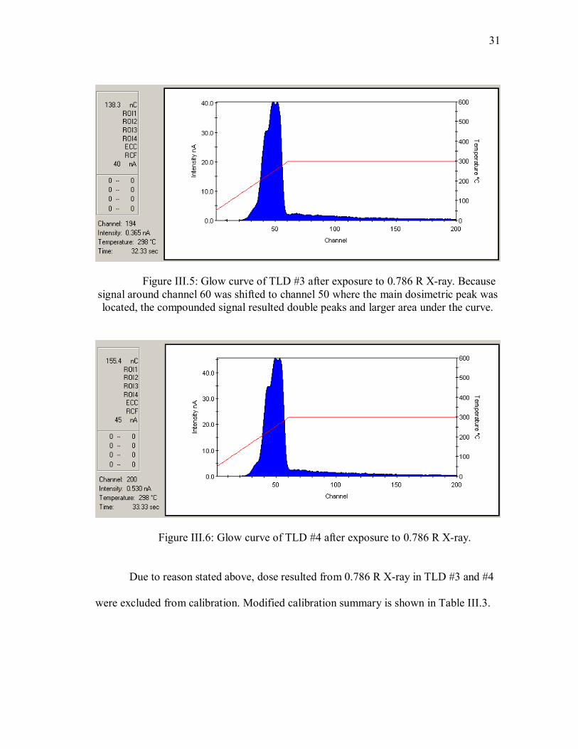
Figure III.5: Glow curve of TLD #3 after exposure to 0.786 R X-ray. Because signal around channel 60 was shifted to channel 50 where the main dosimetric peak was located, the compounded signal resulted double peaks and larger area under the curve.
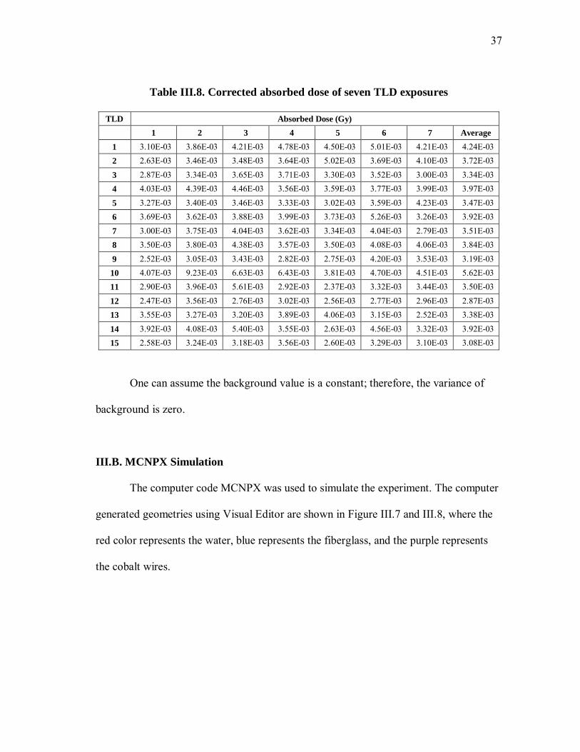
Figure III.6: Glow curve of TLD #4 after exposure to 0.786 R X-ray.
Due to reason stated above, dose resulted from 0.786 R X-ray in TLD #3 and #4
were excluded from calibration. Modified calibration summary is shown in Table III.3.

32
Table III.3. Modified TLD calibration results
0.786 R 1.086 R 0.786 R 1.086 R Average TLD Number nC nC R/nC R/nC R/nC
1 69.503 70.439 0.011 0.015 0.013 2 76.471 78.060 0.010 0.014 0.012 3 Excluded 81.506 Excluded 0.013 0.013 4 Excluded 77.182 Excluded 0.014 0.014 5 77.645 81.224 0.010 0.013 0.012 6 70.431 96.154 0.011 0.011 0.011 7 62.562 53.368 0.013 0.020 0.016 8 50.077 59.276 0.016 0.018 0.017 9 71.778 78.165 0.011 0.014 0.012
10 48.949 61.703 0.016 0.018 0.017 11 89.655 82.768 0.009 0.013 0.011 12 73.571 68.460 0.011 0.016 0.013 13 65.637 75.735 0.012 0.014 0.013 14 62.697 64.288 0.013 0.017 0.015 15 90.726 75.560 0.009 0.014 0.012
Average 69.977 73.593
Once calibrated, the TLDs were placed inside the incubator to map the radiation
field. During a period of thirty days, seven sets of measurements were performed, and
each measurement lasted eight hours. The measurement results are shown in Table III.4,
and their glow curves are shown in Appendix G.

33
Table III.4. Results of seven different exposures measured in nanocoulombs (nC)
TLD Exposure (nC) 1 2 3 4 5 6 7 Average
1 30.266 36.922 40.061 44.985 42.549 43.974 36.940 39.385 2 28.324 36.261 36.458 37.929 51.090 35.040 39.025 37.732 3 28.293 32.424 35.140 35.678 32.036 30.903 26.341 31.545 4 35.695 38.666 39.211 31.839 32.099 30.690 32.503 34.386 5 34.432 35.622 36.234 34.981 32.001 34.126 40.233 35.376 6 41.909 41.197 43.829 45.046 42.275 54.519 33.804 43.226 7 23.915 29.266 31.337 28.303 26.346 28.810 19.903 26.840 8 25.812 27.858 31.780 26.331 25.827 27.356 27.265 27.461 9 27.244 32.325 35.968 30.157 29.515 39.922 33.583 32.673 10 29.654 64.272 46.866 45.499 27.918 31.512 30.296 39.431 11 33.685 44.726 61.814 33.874 28.220 34.467 35.712 38.928 12 24.736 34.329 27.306 29.573 25.570 24.301 25.965 27.397 13 34.232 31.814 31.192 37.251 38.716 27.626 22.147 31.854 14 32.495 33.709 43.723 29.650 22.633 34.701 25.272 31.740 15 27.878 34.153 33.583 37.223 28.011 31.247 29.468 31.652
The original TLD exposures were measured in nanocoulombs (nC), however,
using calibration factors from Table III.3, one can convert the free-space exposure (X)
unit from nanocoulomb (nC) to roentgen (R). The converted exposure is summarized in
Table III.5.

34
Table III.5. Results of seven different exposures measured in roentgens (R)
TLD Exposure ( R) 1 2 3 4 5 6 7 Average 1 0.393 0.480 0.521 0.585 0.553 0.572 0.480 0.512 2 0.340 0.435 0.437 0.455 0.613 0.420 0.468 0.453 3 0.368 0.422 0.457 0.464 0.416 0.402 0.342 0.410 4 0.500 0.541 0.549 0.446 0.449 0.430 0.455 0.481 5 0.413 0.427 0.435 0.420 0.384 0.410 0.483 0.425 6 0.461 0.453 0.482 0.496 0.465 0.600 0.372 0.475 7 0.383 0.468 0.501 0.453 0.422 0.461 0.318 0.429 8 0.439 0.474 0.540 0.448 0.439 0.465 0.464 0.467 9 0.327 0.388 0.432 0.362 0.354 0.479 0.403 0.392
10 0.504 1.093 0.797 0.773 0.475 0.536 0.515 0.670 11 0.371 0.492 0.680 0.373 0.310 0.379 0.393 0.428 12 0.322 0.446 0.355 0.384 0.332 0.316 0.338 0.356 13 0.445 0.414 0.405 0.484 0.503 0.359 0.288 0.414 14 0.487 0.506 0.656 0.445 0.339 0.521 0.379 0.476 15 0.335 0.410 0.403 0.447 0.336 0.375 0.354 0.380
To obtain the absorbed dose (Da) from these exposures (X), one must change the
exposure unit from roentgen (R) to coulomb per kilogram (C/kg) by using Equation 13
before relating exposure to dose by Equation 14,
1 R = 2.58E-4 C/kg (13)
a
a eWXD
* (14)
where Da is absorbed dose in Gy, X is the exposure in C/kg, and (W /e)a is the mean
energy per unit charge released, having the value 33.97 J/C in air under room condition.
The absorbed dose derived by above method is summarized in Table III.6.

35
Table III.6. Absorbed dose of seven TLD exposures
TLD Absorbed Dose (Gy)
1 2 3 4 5 6 7 Average
1 3.45E-03 4.21E-03 4.56E-03 5.13E-03 4.85E-03 5.01E-03 4.21E-03 4.49E-03
2 2.98E-03 3.81E-03 3.83E-03 3.99E-03 5.37E-03 3.69E-03 4.10E-03 3.97E-03
3 3.22E-03 3.69E-03 4.00E-03 4.06E-03 3.65E-03 3.52E-03 3.00E-03 3.59E-03
4 4.38E-03 4.74E-03 4.81E-03 3.91E-03 3.94E-03 3.77E-03 3.99E-03 4.22E-03
5 3.62E-03 3.75E-03 3.81E-03 3.68E-03 3.37E-03 3.59E-03 4.23E-03 3.72E-03
6 4.04E-03 3.97E-03 4.23E-03 4.34E-03 4.08E-03 5.26E-03 3.26E-03 4.17E-03
7 3.35E-03 4.10E-03 4.39E-03 3.97E-03 3.69E-03 4.04E-03 2.79E-03 3.76E-03
8 3.85E-03 4.15E-03 4.73E-03 3.92E-03 3.85E-03 4.08E-03 4.06E-03 4.09E-03
9 2.87E-03 3.40E-03 3.78E-03 3.17E-03 3.10E-03 4.20E-03 3.53E-03 3.44E-03
10 4.42E-03 9.58E-03 6.98E-03 6.78E-03 4.16E-03 4.70E-03 4.51E-03 5.87E-03
11 3.25E-03 4.31E-03 5.96E-03 3.27E-03 2.72E-03 3.32E-03 3.44E-03 3.75E-03
12 2.82E-03 3.91E-03 3.11E-03 3.37E-03 2.91E-03 2.77E-03 2.96E-03 3.12E-03
13 3.90E-03 3.62E-03 3.55E-03 4.24E-03 4.41E-03 3.15E-03 2.52E-03 3.63E-03
14 4.27E-03 4.43E-03 5.75E-03 3.90E-03 2.98E-03 4.56E-03 3.32E-03 4.17E-03 15 2.93E-03 3.59E-03 3.53E-03 3.91E-03 2.95E-03 3.29E-03 3.10E-03 3.33E-03
Because the experiment location (beam port 4 on Lower Research Level at the
Nuclear Science Center, TAMU) is near the vicinity of a nuclear reactor, one should
consider the effects of background radiation from the reactor on TLD results. Based on a
survey with a digital ion chamber (SN# 11332/2109), the experiment location had a
background exposure rate of 42 mR/h when then reactor is operating at maximum power
(1 MW), and a background exposure rate of 37 mR/h when the reactor is shutdown.
Records from the reactor log showed that the reactor was operating at maximum power
during the first five exposures; was shutdown during the sixth measurement; and was
operating at low power during the seventh measurement. A more detailed summary of
reactor operation is shown in Table III.7.

36
Table III.7. Summary of reactor operations from 6/14/10 to 7/12/10
Measurement # Date Rx Operating Power Duration 1 6/14/2010 1 MW all day 2 6/17/2010 1 MW all day 3 6/22/2010 1 MW all day 4 6/25/2010 1 MW all day 5 6/30/2010 1 MW all day 6 7/5/2010 Shutdown shutdown all day 7 7/12/2010 100 W 2:26 pm - 5:08 pm
On 7/12/2010, the reactor was operating at low power (0.1% of maximum) and
was only partially operating when the measurements were in progress. For this reason,
the reactor can be considered shutdown for measurement #7. The background exposure
rate difference between reactor operating and not operating is 5 mR/h (inside of the
incubator). Using methods described earlier in this section, the background radiation
from the reactor would result 3.50E-4 Gy in eight hours. The corrected eight hour
absorbed dose of the fifteen TLDs is summarized in Table III.8.
37
Table III.8. Corrected absorbed dose of seven TLD exposures
TLD Absorbed Dose (Gy) 1 2 3 4 5 6 7 Average
1 3.10E-03 3.86E-03 4.21E-03 4.78E-03 4.50E-03 5.01E-03 4.21E-03 4.24E-03 2 2.63E-03 3.46E-03 3.48E-03 3.64E-03 5.02E-03 3.69E-03 4.10E-03 3.72E-03
3 2.87E-03 3.34E-03 3.65E-03 3.71E-03 3.30E-03 3.52E-03 3.00E-03 3.34E-03 4 4.03E-03 4.39E-03 4.46E-03 3.56E-03 3.59E-03 3.77E-03 3.99E-03 3.97E-03
5 3.27E-03 3.40E-03 3.46E-03 3.33E-03 3.02E-03 3.59E-03 4.23E-03 3.47E-03 6 3.69E-03 3.62E-03 3.88E-03 3.99E-03 3.73E-03 5.26E-03 3.26E-03 3.92E-03
7 3.00E-03 3.75E-03 4.04E-03 3.62E-03 3.34E-03 4.04E-03 2.79E-03 3.51E-03 8 3.50E-03 3.80E-03 4.38E-03 3.57E-03 3.50E-03 4.08E-03 4.06E-03 3.84E-03
9 2.52E-03 3.05E-03 3.43E-03 2.82E-03 2.75E-03 4.20E-03 3.53E-03 3.19E-03 10 4.07E-03 9.23E-03 6.63E-03 6.43E-03 3.81E-03 4.70E-03 4.51E-03 5.62E-03 11 2.90E-03 3.96E-03 5.61E-03 2.92E-03 2.37E-03 3.32E-03 3.44E-03 3.50E-03
12 2.47E-03 3.56E-03 2.76E-03 3.02E-03 2.56E-03 2.77E-03 2.96E-03 2.87E-03 13 3.55E-03 3.27E-03 3.20E-03 3.89E-03 4.06E-03 3.15E-03 2.52E-03 3.38E-03
14 3.92E-03 4.08E-03 5.40E-03 3.55E-03 2.63E-03 4.56E-03 3.32E-03 3.92E-03 15 2.58E-03 3.24E-03 3.18E-03 3.56E-03 2.60E-03 3.29E-03 3.10E-03 3.08E-03
One can assume the background value is a constant; therefore, the variance of
background is zero.
III.B. MCNPX Simulation
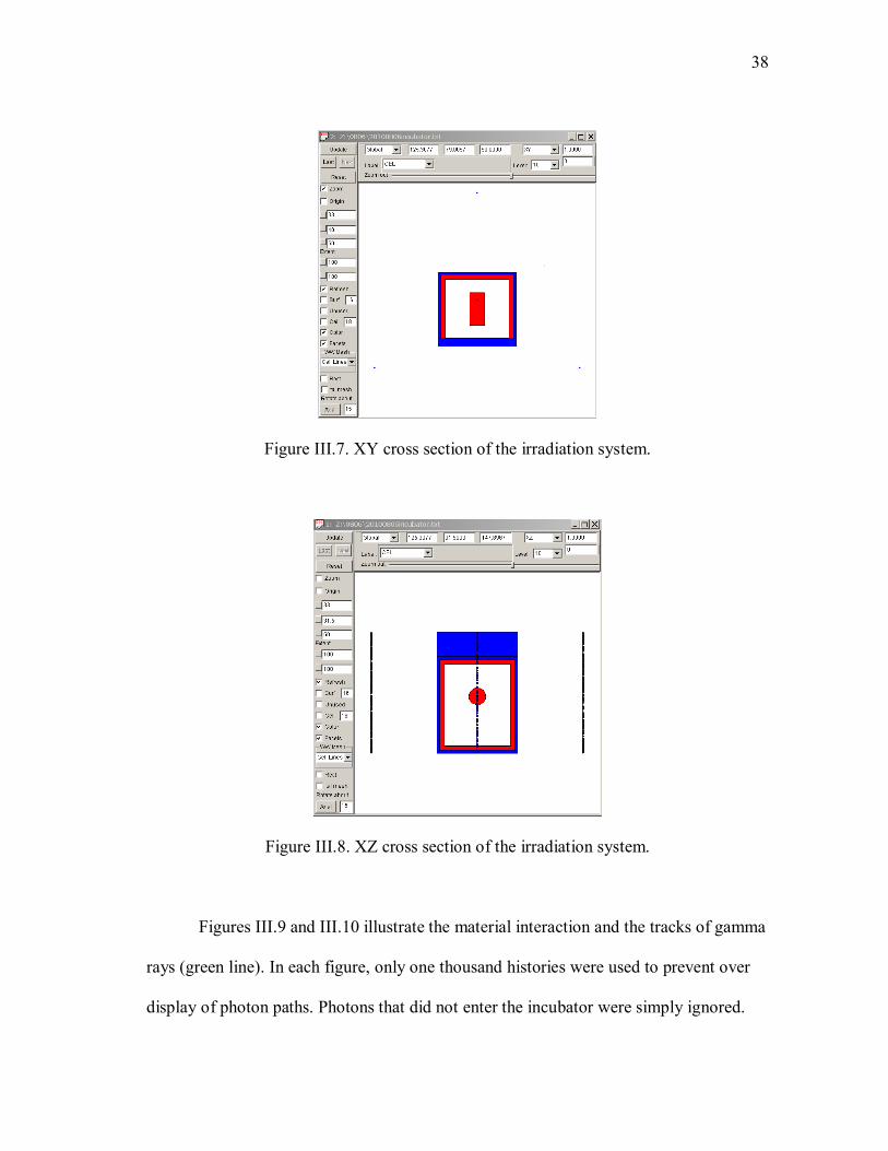
The computer code MCNPX was used to simulate the experiment. The computer
generated geometries using Visual Editor are shown in Figure III.7 and III.8, where the
red color represents the water, blue represents the fiberglass, and the purple represents
the cobalt wires.
38
Figure III.7. XY cross section of the irradiation system.
Figure III.8. XZ cross section of the irradiation system.
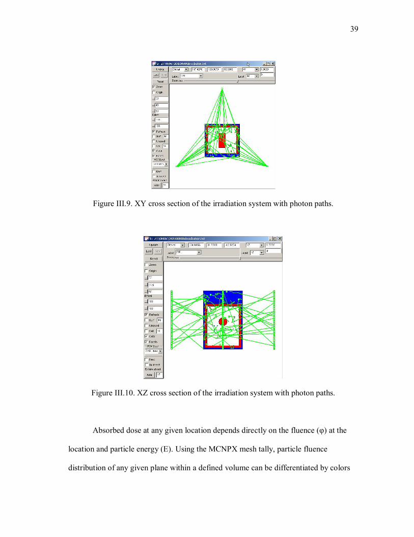
Figures III.9 and III.10 illustrate the material interaction and the tracks of gamma
rays (green line). In each figure, only one thousand histories were used to prevent over
display of photon paths. Photons that did not enter the incubator were simply ignored.
39
Figure III.9. XY cross section of the irradiation system with photon paths.
Figure III.10. XZ cross section of the irradiation system with photon paths.
Absorbed dose at any given location depends directly on the fluence (φ) at the
location and particle energy (E). Using the MCNPX mesh tally, particle fluence
distribution of any given plane within a defined volume can be differentiated by colors
40
(Guan, 2009). To visualize the fluence inside the incubator space, seven planes which
contained various points of interest were chosen. Amongst them, four were horizontal
planes at different elevations and three were vertical planes at different depths. One
hundred million histories were used in the mesh tally to simulate the particle fluence.
Plane A (contained point # 1, 2, 3, 4), B (contained point # 5, 6, 7, 8), C
(contained point # 9, 10, 11, 12) and D (contained point # 13, 14, 15) were horizontal
planes. In terms of elevations, Plane A was the highest, positioned at the very top of
incubator interior; Plane B was middle plane, dividing the interior space into two equal
halves horizontally; Plane C was the lowest, positioned at the bottom of incubator
interior; Plane D was positioned 2 cm above Plane B.
Plane E (contained points # 3, 4, 7, 8, 11, 12), F (contained point #14) and G
(contained points # 1, 2, 5, 6, 9, 10) were vertical planes at different depths. Amongst
them, Plane E was the front-most, positioned right behind the incubator door. Plane F
was the middle plane. It divided the interior space into two equal halves vertically. Plane
G was the farthest vertical plane away from the door, positioned right in front of the
incubator back wall.
41
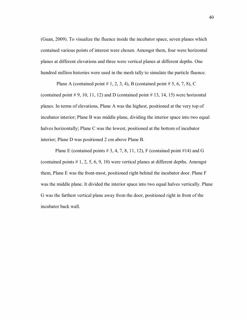
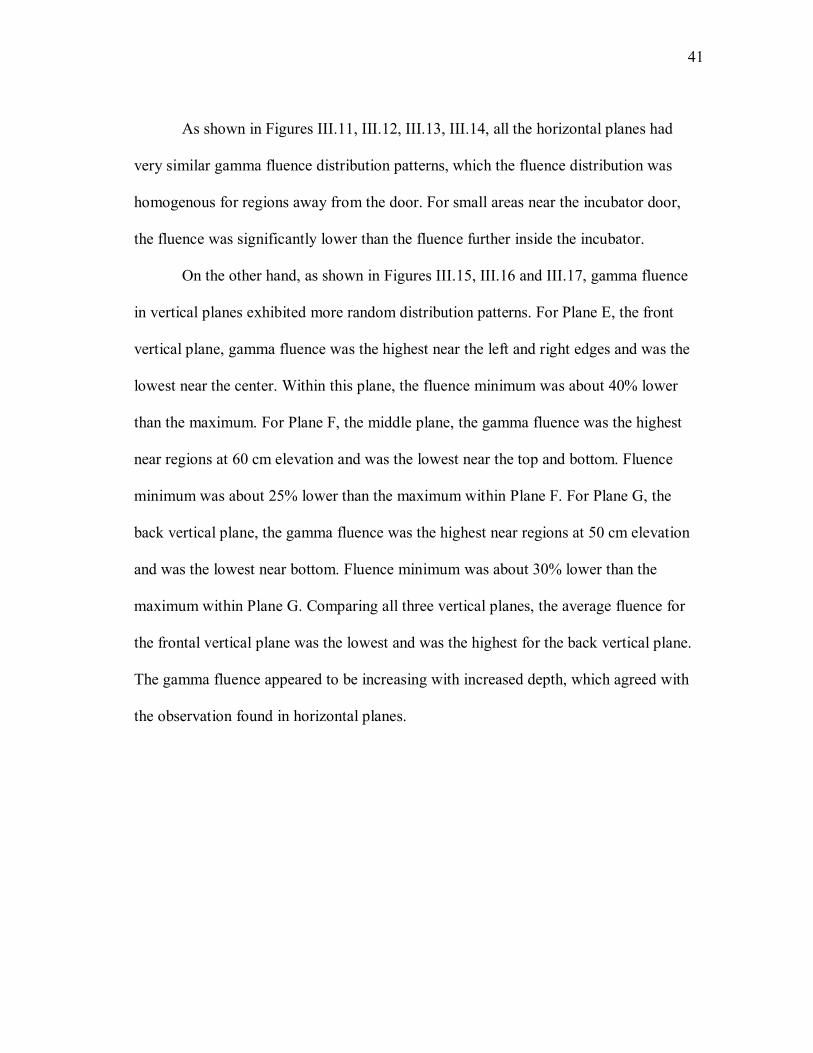
As shown in Figures III.11, III.12, III.13, III.14, all the horizontal planes had
very similar gamma fluence distribution patterns, which the fluence distribution was
homogenous for regions away from the door. For small areas near the incubator door,
the fluence was significantly lower than the fluence further inside the incubator.
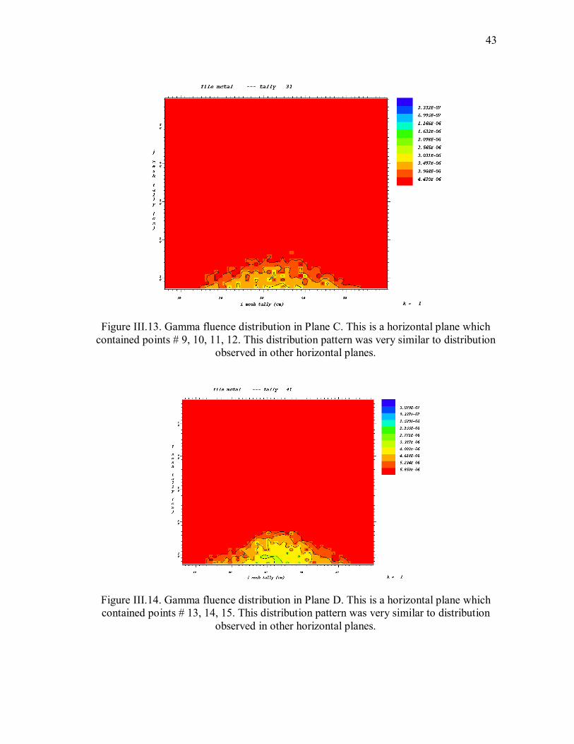
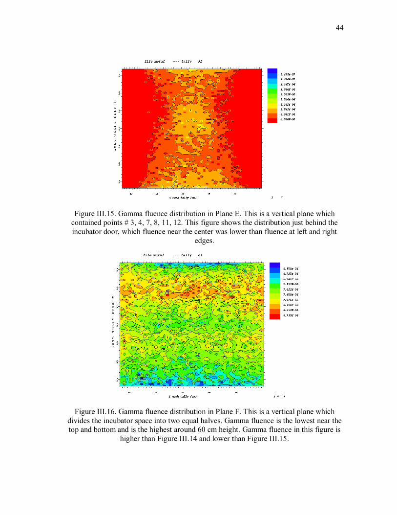
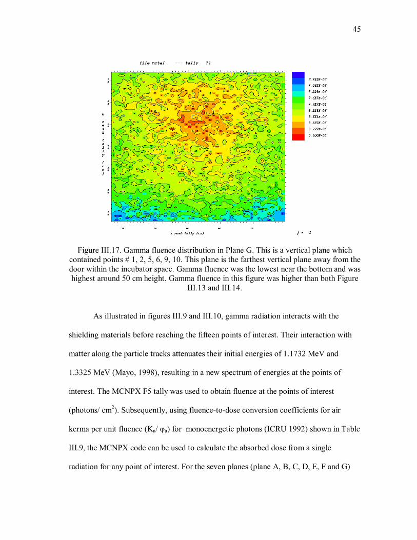
On the other hand, as shown in Figures III.15, III.16 and III.17, gamma fluence
in vertical planes exhibited more random distribution patterns. For Plane E, the front
vertical plane, gamma fluence was the highest near the left and right edges and was the
lowest near the center. Within this plane, the fluence minimum was about 40% lower
than the maximum. For Plane F, the middle plane, the gamma fluence was the highest
near regions at 60 cm elevation and was the lowest near the top and bottom. Fluence
minimum was about 25% lower than the maximum within Plane F. For Plane G, the
back vertical plane, the gamma fluence was the highest near regions at 50 cm elevation
and was the lowest near bottom. Fluence minimum was about 30% lower than the
maximum within Plane G. Comparing all three vertical planes, the average fluence for
the frontal vertical plane was the lowest and was the highest for the back vertical plane.
The gamma fluence appeared to be increasing with increased depth, which agreed with
the observation found in horizontal planes.

42
Figure III.11. Gamma fluence distribution in Plane A. This is a horizontal plane, which contained points # 1, 2, 3, 4. The distribution were mostly homogeneous, except a small
area near the door, which was about 50% lower than the rear area. This distribution pattern was very similar to distribution observed in other horizontal planes.
Figure III.12. Gamma fluence distribution in Plane B. This is a horizontal plane which contained points # 5, 6, 7, 8. This distribution pattern was very similar to distribution
observed in other horizontal planes.
43
Figure III.13. Gamma fluence distribution in Plane C. This is a horizontal plane which contained points # 9, 10, 11, 12. This distribution pattern was very similar to distribution
observed in other horizontal planes.
Figure III.14. Gamma fluence distribution in Plane D. This is a horizontal plane which contained points # 13, 14, 15. This distribution pattern was very similar to distribution
observed in other horizontal planes.
44
Figure III.15. Gamma fluence distribution in Plane E. This is a vertical plane which contained points # 3, 4, 7, 8, 11, 12. This figure shows the distribution just behind the incubator door, which fluence near the center was lower than fluence at left and right
edges.
Figure III.16. Gamma fluence distribution in Plane F. This is a vertical plane which divides the incubator space into two equal halves. Gamma fluence is the lowest near the top and bottom and is the highest around 60 cm height. Gamma fluence in this figure is
higher than Figure III.14 and lower than Figure III.15.
45
Figure III.17. Gamma fluence distribution in Plane G. This is a vertical plane which contained points # 1, 2, 5, 6, 9, 10. This plane is the farthest vertical plane away from the door within the incubator space. Gamma fluence was the lowest near the bottom and was highest around 50 cm height. Gamma fluence in this figure was higher than both Figure
III.13 and III.14.
As illustrated in figures III.9 and III.10, gamma radiation interacts with the
shielding materials before reaching the fifteen points of interest. Their interaction with
matter along the particle tracks attenuates their initial energies of 1.1732 MeV and
1.3325 MeV (Mayo, 1998), resulting in a new spectrum of energies at the points of
interest. The MCNPX F5 tally was used to obtain fluence at the points of interest
(photons/ cm2). Subsequently, using fluence-to-dose conversion coefficients for air
kerma per unit fluence (Ka/ φa) for monoenergetic photons (ICRU 1992) shown in Table
III.9, the MCNPX code can be used to calculate the absorbed dose from a single
radiation for any point of interest. For the seven planes (plane A, B, C, D, E, F and G)
46
mentioned above, the distributions of averaged absorbed dose from a single source
particle are shown in Figures III.18, III.19, III.20, III.21, III.22, III.23 and III.24.
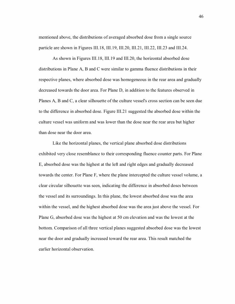
As shown in Figures III.18, III.19 and III.20, the horizontal absorbed dose
distributions in Plane A, B and C were similar to gamma fluence distributions in their
respective planes, where absorbed dose was homogeneous in the rear area and gradually
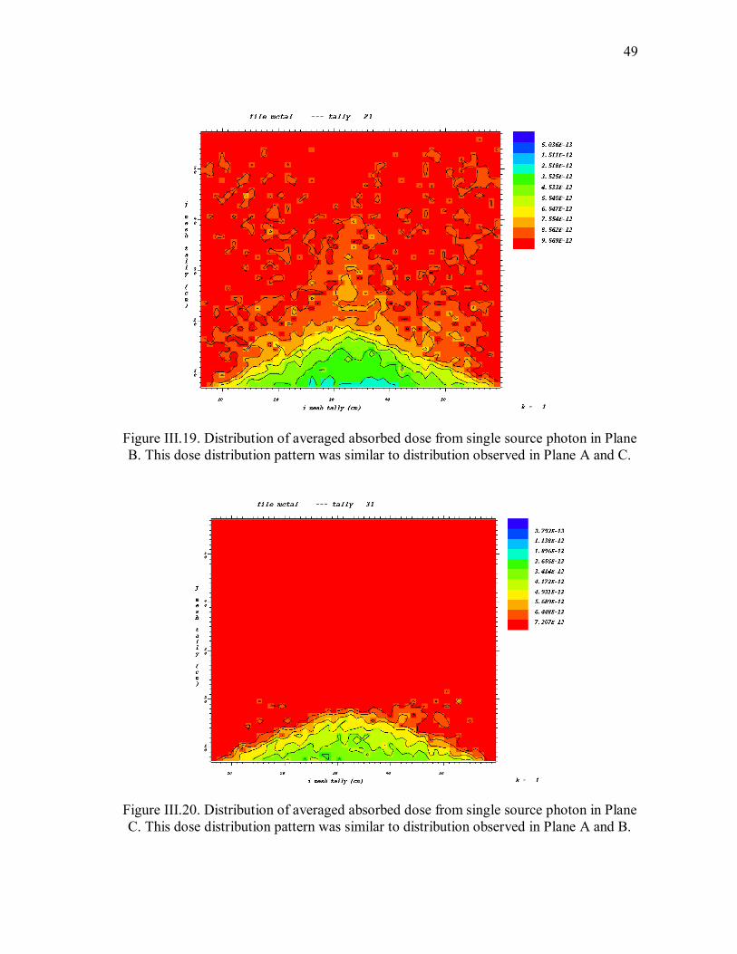
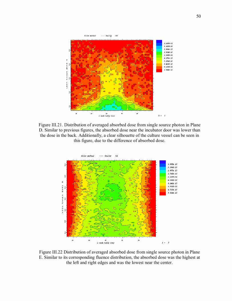
decreased towards the door area. For Plane D, in addition to the features observed in
Planes A, B and C, a clear silhouette of the culture vessel's cross section can be seen due
to the difference in absorbed dose. Figure III.21 suggested the absorbed dose within the
culture vessel was uniform and was lower than the dose near the rear area but higher
than dose near the door area.
Like the horizontal planes, the vertical plane absorbed dose distributions
exhibited very close resemblance to their corresponding fluence counter parts. For Plane
E, absorbed dose was the highest at the left and right edges and gradually decreased
towards the center. For Plane F, where the plane intercepted the culture vessel volume, a
clear circular silhouette was seen, indicating the difference in absorbed doses between
the vessel and its surroundings. In this plane, the lowest absorbed dose was the area
within the vessel, and the highest absorbed dose was the area just above the vessel. For
Plane G, absorbed dose was the highest at 50 cm elevation and was the lowest at the
bottom. Comparison of all three vertical planes suggested absorbed dose was the lowest
near the door and gradually increased toward the rear area. This result matched the
earlier horizontal observation.

47
Table III.9. Conversion coefficients for air kerma per unit fluence (Ka/ φa) for monoenergetic photons (ICRU 1992)
Photon energy (MeV) Ka/Φ (pGy cm2)
0.010 7.430 0.015 3.120 0.020 1.680 0.030 0.721 0.040 0.429 0.050 0.323 0.060 0.289 0.080 0.307 0.100 0.371 0.150 0.599 0.200 0.856 0.300 1.380 0.400 1.890 0.500 2.380 0.600 2.840 0.800 3.690 1.000 4.470 1.500 6.140 2.000 7.550 3.000 9.960 4.000 12.100 5.000 14.100 6.000 16.100 8.000 20.100 10.000 24.000

48
Figure III.18. Distribution of averaged absorbed dose from single source photon in Plane A. Similar to gamma fluence distribution, the averaged absorbed dose was more
homogeneous in the rear. Additionally, dose near the incubator door was significantly lower than dose in the back. This distribution pattern was very similar to distribution
observed in other horizontal planes.
49
Figure III.19. Distribution of averaged absorbed dose from single source photon in Plane B. This dose distribution pattern was similar to distribution observed in Plane A and C.
Figure III.20. Distribution of averaged absorbed dose from single source photon in Plane C. This dose distribution pattern was similar to distribution observed in Plane A and B.
50
Figure III.21. Distribution of averaged absorbed dose from single source photon in Plane D. Similar to previous figures, the absorbed dose near the incubator door was lower than the dose in the back. Additionally, a clear silhouette of the culture vessel can be seen in
this figure, due to the difference of absorbed dose.
Figure III.22 Distribution of averaged absorbed dose from single source photon in Plane E. Similar to its corresponding fluence distribution, the absorbed dose was the highest at
the left and right edges and was the lowest near the center.

51
Figure III.23. Distribution of averaged absorbed dose from single source photon in Plane F. A clear silhouette of the culture vessel can be seen in this figure, due to differences in absorbed doses between the vessel and its surroundings. Magnitude wise, the absorbed
dose in this figure was higher than Figure III.22 but lower than Figure III.24.
Figure III.24. Distribution of averaged absorbed dose from single source photon in Plane G. Absorbed dose was the lowest near the bottom and was highest around 50 cm height.
The absorbed dose in this figure was higher than both Figure III.22 and III.23.
52
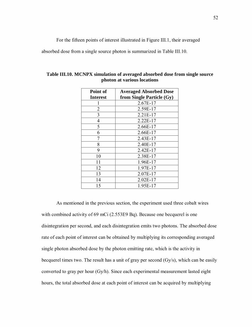
For the fifteen points of interest illustrated in Figure III.1, their averaged
absorbed dose from a single source photon is summarized in Table III.10.
Table III.10. MCNPX simulation of averaged absorbed dose from single source photon at various locations
Point of Interest
Averaged Absorbed Dose from Single Particle (Gy)
1 2.67E-17 2 2.59E-17 3 2.21E-17 4 2.22E-17 5 2.66E-17 6 2.66E-17 7 2.43E-17 8 2.40E-17 9 2.42E-17
10 2.38E-17 11 1.96E-17 12 1.97E-17 13 2.07E-17 14 2.02E-17 15 1.95E-17
As mentioned in the previous section, the experiment used three cobalt wires
with combined activity of 69 mCi (2.553E9 Bq). Because one becquerel is one
disintegration per second, and each disintegration emits two photons. The absorbed dose
rate of each point of interest can be obtained by multiplying its corresponding averaged
single photon absorbed dose by the photon emitting rate, which is the activity in
becquerel times two. The result has a unit of gray per second (Gy/s), which can be easily
converted to gray per hour (Gy/h). Since each experimental measurement lasted eight
hours, the total absorbed dose at each point of interest can be acquired by multiplying
53
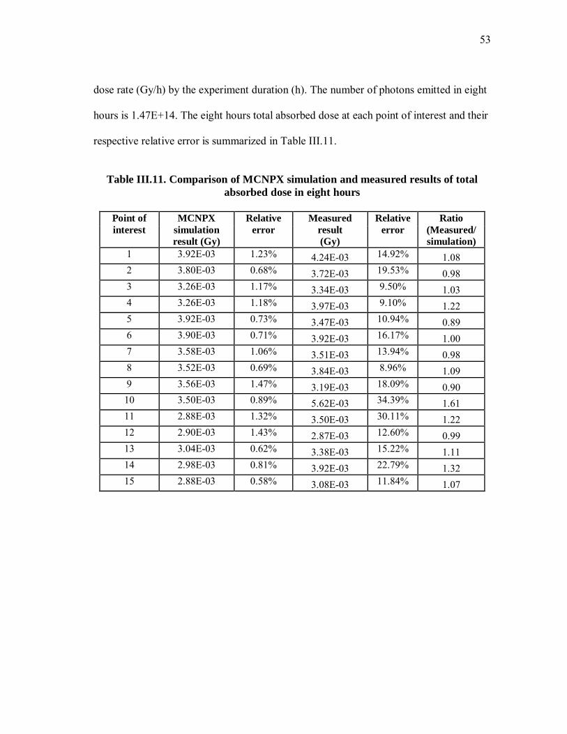
dose rate (Gy/h) by the experiment duration (h). The number of photons emitted in eight
hours is 1.47E+14. The eight hours total absorbed dose at each point of interest and their
respective relative error is summarized in Table III.11.
Table III.11. Comparison of MCNPX simulation and measured results of total
absorbed dose in eight hours
Point of interest
MCNPX simulation result (Gy)
Relative error
Measured result (Gy)
Relative error
Ratio (Measured/ simulation)
1 3.92E-03 1.23% 4.24E-03 14.92% 1.08 2 3.80E-03 0.68% 3.72E-03 19.53% 0.98 3 3.26E-03 1.17% 3.34E-03 9.50% 1.03 4 3.26E-03 1.18% 3.97E-03 9.10% 1.22 5 3.92E-03 0.73% 3.47E-03 10.94% 0.89 6 3.90E-03 0.71% 3.92E-03 16.17% 1.00 7 3.58E-03 1.06% 3.51E-03 13.94% 0.98 8 3.52E-03 0.69% 3.84E-03 8.96% 1.09 9 3.56E-03 1.47% 3.19E-03 18.09% 0.90 10 3.50E-03 0.89% 5.62E-03 34.39% 1.61 11 2.88E-03 1.32% 3.50E-03 30.11% 1.22 12 2.90E-03 1.43% 2.87E-03 12.60% 0.99 13 3.04E-03 0.62% 3.38E-03 15.22% 1.11 14 2.98E-03 0.81% 3.92E-03 22.79% 1.32 15 2.88E-03 0.58% 3.08E-03 11.84% 1.07

54
IV. DISCUSSION
Due to the inherent errors of performing the actual experiment, such as the
uneven heating in the TLD reader and radiation from the reactor, the MCNPX
simulation is considered more accurate in comparison. Based on results shown in
previous sections, the data from the actual experiment agreed with the MCNPX
simulation in both dose distribution pattern and magnitude.
In the MCNPX simulation, as evidenced in Figures III.18, III.19 and III.20, the
absorbed dose distributions are mostly uniform for spaces away from the incubator door,
which made up the majority of the incubator volume. All three figures showed the dose
was lowest right behind the center line of incubator door, and gradually increased toward
the back and left and right edges. Based on readings from the three figures, the dose
minimum was 50% - 60% lower than the dose maximum in their respective horizontal
planes. This distribution pattern can be explained by the difference in stopping power for
different materials. The door and the other walls have about the same thickness,
however, the door is composed only of fiberglass while the walls are composed of water
and fiberglass. Because fiberglass has higher Z number than water, hence, it has higher
attenuation factor. As a result, photons that are attenuated by the door which has a
thicker fiberglass layer have lower energy, thus resulting in a lower interior dose behind
the door. Despite this large difference in magnitude around the door area, all the
horizontal figures showed that only a small percentage (around 10%) of the incubator
volume was affected by the door. For space not affected by the door, dose distribution

55
can be considered uniform. This was evidenced in Table IV.1, dose in the rear space was
only 15% higher than dose in front on average, and for individual Planes A, B and C,
differences for dose at all points of interest were well below 20%.
Table IV.1. Comparison of total absorbed dose between frontal and rear TLDs for
the actual experiment and simulation
Front vs. Rear Simulated Actual 3 vs. 2 14.21% 10.07% Plane A 4 vs. 1 16.84% 6.33% 7 vs. 6 8.21% 10.30% Plane B 8 vs. 5 10.20% -10.69%
11 vs. 10 17.71% 37.72% Plane C 12 vs. 9 18.54% 9.88% average 14.29% 10.60%
Such dose distribution patterns were also observed in the actual experiment.
Most of the frontal TLDs (# 3, 4, 7, 8, 11 and 12) recorded lower doses than the TLDs in
the back (# 1, 2, 5, 6, 9 and 10) . Magnitude-wise, as shown in Table IV.1, the actual
experiment exhibited an even more uniform distribution pattern than the MCNP
simulation. On average, dose in the rear space was only 10% higher than dose in the
front, compared to the 15% in simulation.
The upper horizontal plane (Plane A), which TLD # 1, 2, 3 and 4 rest upon, was
comparable to its corresponding MCNPX plane profile, where TLD # 3 (front, right) is
lower than TLD # 2 (rear, right) by 10.07% versus the 14.21% in the simulation and
TLD # 4 (front, left) is lower than TLD # 1 (rear, left) by 6.33% versus the 16.84% in
the simulation.
56
The middle (Plane B) and the lower (Plane C) horizontal plane exhibit similar
distribution patterns, where frontal doses are just slightly lower than the rear doses. The
only exceptions were TLD # 8 (middle, right, front) being 10.69% higher than TLD # 5
(middle, right, rear).
Magnitude-wise, the dose measured in the actual experiment was very similar to
the simulation value with some minor differences. Table III.11 showed the majority of
experiment/simulation ratios was close to one (ranging between 0.89 to 1.32), excluding
TLD#10, which had a ratio of 1.61. This inconsistency was likely due to the location of
TLD#10 being closest to the nuclear reactor during the experiment, but it can also be
possibly caused by a combination of several factors, namely, TLD errors and the
inconsistency of incubator material distribution.
The unusually large dose reading in TLD#10, along with abnormal ratio between
TLD #8 and #5, suggests the possibility of TLD errors. Subsequent post-experiment tests
placed the fifteen TLDs in the same spot within the incubator for eight hours, and the
result showed abnormal exposure readings for the three TLDs in question, hence
confirming some degree of inconsistency amongst the TLD chips. The result of post-
experiment tests can be found in Appendix B.
Another explanation for actual dose being different than the simulation is the
background radiation from the reactor. As shown in previous calculations, radiations
from the cobalt wires are responsible for the vast majority of radiation dose. However,
background radiation was accountable for about 10% of the total dose registered in the
TLD chips. Therefore, background radiation can be considered at least a minor factor

57
causing the discrepancy, especially for TLD#10 since it was the nearest to the nuclear
reactor.
The final explanation is the inconsistency of incubator material. In MCNPX
simulation, only three materials, namely, stainless steel, fiberglass and water were
considered as the incubator building materials. However, in reality, there may be more
types of materials that were used to construct the incubator, such as tin coating, copper
wiring and/or other metallic components. These materials have the potential to influence
the radiation field differently due to the difference in attenuation factors.
Despite the small discrepancies between the MCNPX simulation and the actual
experiment, the majority of the points of interest shared many similarities in terms of
distribution pattern and magnitude. Both the simulation and the experiment suggested
the dose distribution in rear incubator volume was uniform. Due to striking resemblance
between the simulation and the experiment, one can further imply that if the bacteria
culture vessel was available at the time of experiment, the dose distribution within its
boundary would also be uniform, as suggested in the MCNPX simulation.
58
V. CONCLUSION AND FUTURE WORK
V.A Conclusion
The objective of this research was to create a uniform radiation environment with
a dose rate below 1 mGy/h. To accomplish this task, MCNPX simulation was first used
to test the feasibility of constructing such environment with available equipment. Once
the feasibility was confirmed, an actual experiment was carried out by carefully
following the simulation. To ensure the experiment consistency, fifteen TLD chips were
used to monitor the radiation field for a duration of thirty days. The actual dose
distribution pattern was observed to be similar to its simulation counterpart, where the
dose rate near the incubator door was lower than the dose rate near the rear. A uniform
radiation field was achieved in the rear space of the incubator, which accounted for the
majority of the incubator volume. Furthermore, the actual dose rate had a range from
0.298 to 0.696 mGy/h, hence meeting the initial design criteria.
V.B Future Work
Several improvements can be made to enhance the accuracy of future
experiments. First is TLD selection. As TLD chip detection efficiency depends on its
material makeup, TLDs from different manufacturer will have some difference in
material composition, hence they may produce inconsistencies in dose readings. Even
for TLDs from the same manufacturer, there are still significant variations, known as
"batch variations". Therefore, mix matching of TLDs from different manufacturer is not

59
recommended. If financially possible, one can irradiate a large number of TLDs and
select those with the same response to overcome the inherent variations.
The second recommendation concerns experiment site selection; an ideal site for
this experiment is a location with very low background radiation. Places near the nuclear
reactor or radioactive materials are not recommended.
The third recommendation is to spread the source more evenly around the
incubator. Within financial constraints, one can use more cobalt wires with less activity
to create a more uniform radiation field. For example, using six wires each with half the
activity would result a more homogeneous radiation field than the setup used in this
research. If the experiment site allows liquid to be as used radiation source, one can use
the MIT approach mentioned in the introduction section by mixing radioactive material
into liquid and inject the newly created liquid source into the incubator water jacket to
produce an even more uniform radiation field.
The ultimate purpose of this research is to examine the feasibility of constructing
a low-dose irradiation facility to simulate the exposure rates that exist in space. Cosmic
rays consist of protons, alpha particles, beta particles, gamma rays and heavier ions.
Hence, using a gamma source is only the first step to simulate a realistic space
environment on Earth. For particles that have short range, such alpha and heavy ions,
the source may be positioned inside the incubator near the bacterial vessel (target). For
particles that have a longer range, the sources may be positioned outside of the
incubator.
60
REFERENCES
Attix FH. Introduction to radiological physics and radiation dosimetry. New York: John Wiley and Sons; 2004. Beckurts KH, Wirtz K. Neutron physics. New York: Springer-Verlag; 1964. Berger T., Hajek M. TL-efficiency—Overview and experimental results over the years, Radiation Measurements, 43:146-156; 2008. Cucinotta F. Space radiation organ dose for astronauts on past and future missions. Available at http://ntrs.nasa.gov/archive/nasa/casi.ntrs.nasa.gov/20070010704_2007005 310.pdf. Accessed 5 December 2010. Guan F. Design and simulation of a passive-scattering nozzle in proton beam radiotherapy. M.S. thesis, Texas A&M University, College Station; 2009. Howell RW, Goddu M and Rao DV, Design and performance characteristics of an experimental cesium-137 irradiator to simulate internal radionuclide dose rate patterns, Journal of Nuclear Medicine, 38: 727-730; 1997. International Commission on Radiation Units and Measurements (ICRU). Radiation Quantities and Units, ICRU Report 47. Bethesda, MD: Int. Comm. Radiat. Units and Measurement; 1992.
International Commission on Radiological Protection (ICRP). A Framework for Assessing the Impact of Ionising Radiation on Non-human Species, ICRP Publication 91.; 2003. Ishida Y, Takabatake T, Kakinuma S, Doi K, Yamauchi K, Kaminishi M, Kito S, Ohta Y, Amasaki Y, Moritake H, Kokubo T, Nishimura M, Nishikawa T, Hino O, Shimada Y. Genomic and gene expression signatures of radiation in medulloblastomas after low-dose irradiation in Ptch1 heterozygous mice. Carcinogensis 31:1694-1701.; 2010. Mayo RM. Introduction to nuclear concepts for engineers. La Grange Park, IL: American Nuclear Society; 1998. Mihok S. Chronic exposure to gamma radiation of wild populations of meadow voles. Journal of Environmental Radioactivity, 75: 233-266; 2004. Mishev AL, Mavrodiev SC and Stamenov JN. In Martsch IN eds. Frontiers in cosmic rays research, New York: Nova Science Publishers, 35-83; 2004.

61
Mitchel R EJ, Burchart P and Wyatt H. A lower dose threshold for the in vivo protective adaptive response to radiation. Tumorigenesis in chronically exposed normal and Trp53 heterozygous C57BL/6 mice, Radiation Research Society; 170:765-75;2008. Oldenberg, O., Rasmussen, NC. Modern physics for engineers. New York: McGraw-Hill, Inc; 1996. Olipitz W, Hembrador S, Davidson M, Yanch JC, Engelward BP. Development and characterization of a novel variable low dose-rate irradiator for in vivo mouse studies. Health Physics Society, 2010. Rice AJ. Mathematical statistics and data analysis, 2nd ed. Belmont, CA, Duxbury Press; 1995. Shin SC, Lee KM, Kang YM, Kim K, Kim CS, Yang KH, Jin YW, Kim CS, Kim HS. Alteration of cytokine profiles in mice exposed to chronic low-dose ionizing radiation. Biochemical and Biophysical Research Communications, 2010. Simpson JA, Elemental and isotopic composition of the galactic cosmic rays, Nucl. and Particle Sci., 33:323-382; 1983. Thermo Scientific Forma Series II Water Jacketed CO2 Incubator, Thermo Scientific. Available at: http://www.thermoscientific.com/wps/portal/ts/products/detail?productId= 11962287. Accessed 11 February 2011. Tsoulfanidis N., Measurement and detection of radiation, 2nd ed. Washington, DC: Taylor & Francis; 1995. Turner JE. Atoms, radiation and radiation protection, 2nd ed. New York: Wiley & Sons; 1995. Wakeford R, Tawn EJ, The meaning of low dose and low dose-rate. Journal of Radiological Protection, 30: 1-3; 2010.
62
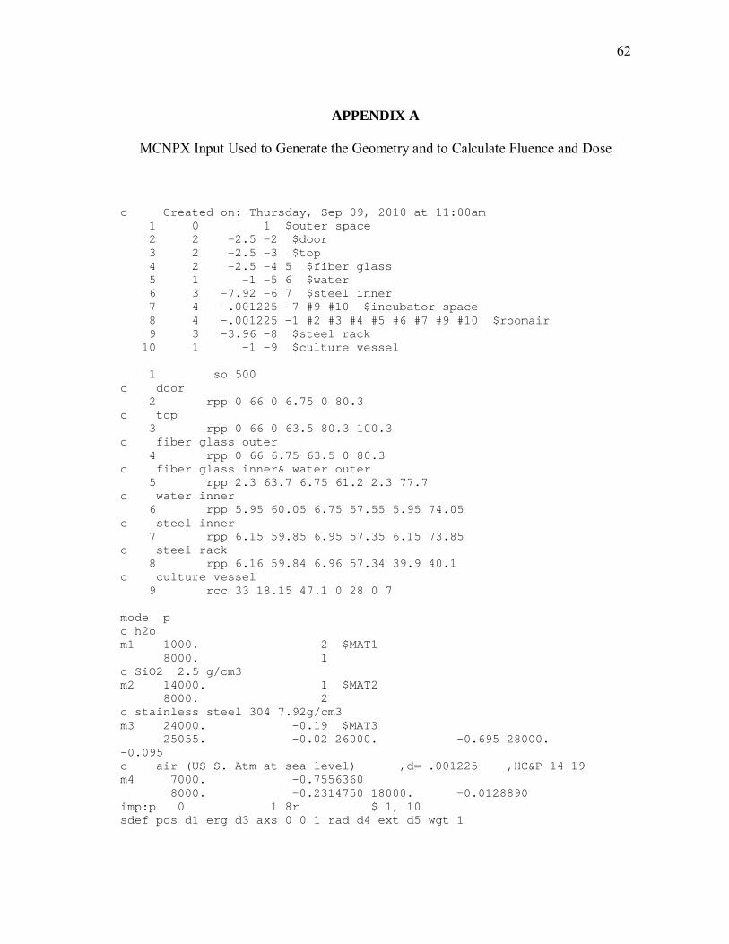
APPENDIX A
MCNPX Input Used to Generate the Geometry and to Calculate Fluence and Dose
c Created on: Thursday, Sep 09, 2010 at 11:00am 1 0 1 $outer space 2 2 -2.5 -2 $door 3 2 -2.5 -3 $top 4 2 -2.5 -4 5 $fiber glass 5 1 -1 -5 6 $water 6 3 -7.92 -6 7 $steel inner 7 4 -.001225 -7 #9 #10 $incubator space 8 4 -.001225 -1 #2 #3 #4 #5 #6 #7 #9 #10 $roomair 9 3 -3.96 -8 $steel rack 10 1 -1 -9 $culture vessel 1 so 500 c door 2 rpp 0 66 0 6.75 0 80.3 c top 3 rpp 0 66 0 63.5 80.3 100.3 c fiber glass outer 4 rpp 0 66 6.75 63.5 0 80.3 c fiber glass inner& water outer 5 rpp 2.3 63.7 6.75 61.2 2.3 77.7 c water inner 6 rpp 5.95 60.05 6.75 57.55 5.95 74.05 c steel inner 7 rpp 6.15 59.85 6.95 57.35 6.15 73.85 c steel rack 8 rpp 6.16 59.84 6.96 57.34 39.9 40.1 c culture vessel 9 rcc 33 18.15 47.1 0 28 0 7 mode p c h2o m1 1000. 2 $MAT1 8000. 1 c SiO2 2.5 g/cm3 m2 14000. 1 $MAT2 8000. 2 c stainless steel 304 7.92g/cm3 m3 24000. -0.19 $MAT3 25055. -0.02 26000. -0.695 28000. -0.095 c air (US S. Atm at sea level) ,d=-.001225 ,HC&P 14-19 m4 7000. -0.7556360 8000. -0.2314750 18000. -0.0128890 imp:p 0 1 8r $ 1, 10 sdef pos d1 erg d3 axs 0 0 1 rad d4 ext d5 wgt 1
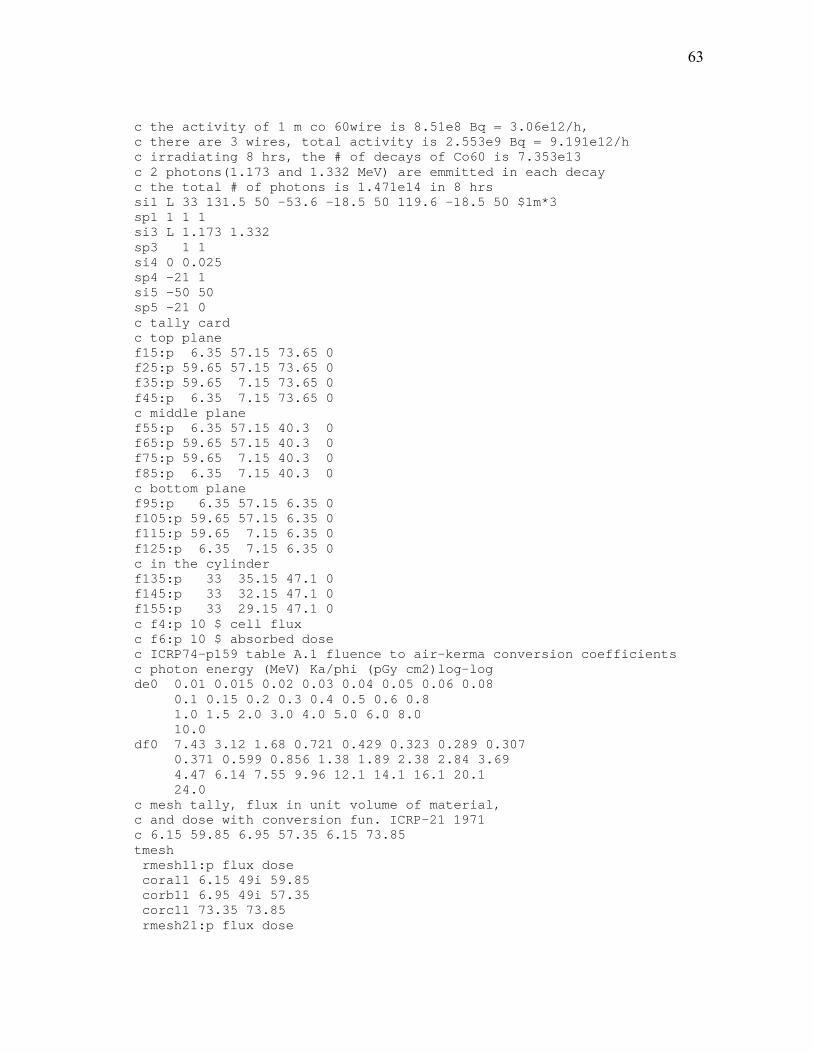
63
c the activity of 1 m co 60wire is 8.51e8 Bq = 3.06e12/h, c there are 3 wires, total activity is 2.553e9 Bq = 9.191e12/h c irradiating 8 hrs, the # of decays of Co60 is 7.353e13 c 2 photons(1.173 and 1.332 MeV) are emmitted in each decay c the total # of photons is 1.471e14 in 8 hrs si1 L 33 131.5 50 -53.6 -18.5 50 119.6 -18.5 50 $1m*3 sp1 1 1 1 si3 L 1.173 1.332 sp3 1 1 si4 0 0.025 sp4 -21 1 si5 -50 50 sp5 -21 0 c tally card c top plane f15:p 6.35 57.15 73.65 0 f25:p 59.65 57.15 73.65 0 f35:p 59.65 7.15 73.65 0 f45:p 6.35 7.15 73.65 0 c middle plane f55:p 6.35 57.15 40.3 0 f65:p 59.65 57.15 40.3 0 f75:p 59.65 7.15 40.3 0 f85:p 6.35 7.15 40.3 0 c bottom plane f95:p 6.35 57.15 6.35 0 f105:p 59.65 57.15 6.35 0 f115:p 59.65 7.15 6.35 0 f125:p 6.35 7.15 6.35 0 c in the cylinder f135:p 33 35.15 47.1 0 f145:p 33 32.15 47.1 0 f155:p 33 29.15 47.1 0 c f4:p 10 $ cell flux c f6:p 10 $ absorbed dose c ICRP74-p159 table A.1 fluence to air-kerma conversion coefficients c photon energy (MeV) Ka/phi (pGy cm2)log-log de0 0.01 0.015 0.02 0.03 0.04 0.05 0.06 0.08 0.1 0.15 0.2 0.3 0.4 0.5 0.6 0.8 1.0 1.5 2.0 3.0 4.0 5.0 6.0 8.0 10.0 df0 7.43 3.12 1.68 0.721 0.429 0.323 0.289 0.307 0.371 0.599 0.856 1.38 1.89 2.38 2.84 3.69 4.47 6.14 7.55 9.96 12.1 14.1 16.1 20.1 24.0 c mesh tally, flux in unit volume of material, c and dose with conversion fun. ICRP-21 1971 c 6.15 59.85 6.95 57.35 6.15 73.85 tmesh rmesh11:p flux dose cora11 6.15 49i 59.85 corb11 6.95 49i 57.35 corc11 73.35 73.85 rmesh21:p flux dose

64
cora21 6.15 49i 59.85 corb21 6.95 49i 57.35 corc21 40.0 40.5 rmesh31:p flux dose cora31 6.15 49i 59.85 corb31 6.95 49i 57.35 corc31 6.0 6.5 rmesh41:p flux dose cora41 6.15 49i 59.85 corb41 6.95 49i 57.35 corc41 46.8 47.3 rmesh51:p flux dose cora51 6.15 49i 59.85 corb51 6.95 7.95 corc51 6.15 66i 73.85 rmesh61:p flux dose cora61 6.15 49i 59.85 corb61 31.65 32.65 corc61 6.15 66i 73.85 rmesh71:p flux dose cora71 6.15 49i 59.85 corb71 56.35 57.35 corc71 6.15 66i 73.85 endmd c running parameters nps 1e8 print prdmp 2j 1

65
APPENDIX B
Results of post-experiment tests
TLD Number
Exposure (nC)
Dose (R)
1 34.756 0.452 2 31.786 0.381 3 24.778 0.248 4 30.910 0.309 5 35.296 0.424 6 30.636 0.337 7 30.760 0.492 8 26.665 0.453 9 31.482 0.378 10 31.264 0.531 11 48.704 0.536 12 28.191 0.366 13 36.526 0.475 14 31.184 0.468 15 30.715 0.369
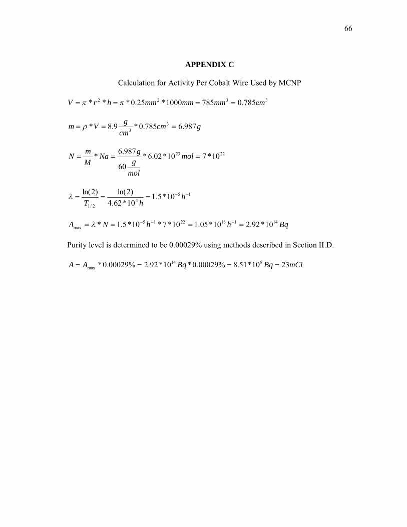
66
APPENDIX C
Calculation for Activity Per Cobalt Wire Used by MCNP
3322 785c.07851000*25.0*** mmmmmmmhrV
gcmcm
gVm 987.6785.0*9.8* 33
2223 10*710*02.6*
60
987.6* mol
molg
gNaMmN
15
42/1
10*5.110*62.4)2ln()2ln( h
hT
BqhhNA 141182215
max 10*92.210*05.110*7*10*5.1* Purity level is determined to be 0.00029% using methods described in Section II.D.
mCiBqBqAA 2310*51.8%00029.0*10*92.2%00029.0* 814max

67
APPENDIX D
Records of Cobalt Wire Neutron Activation Provided by Nuclear Science Center
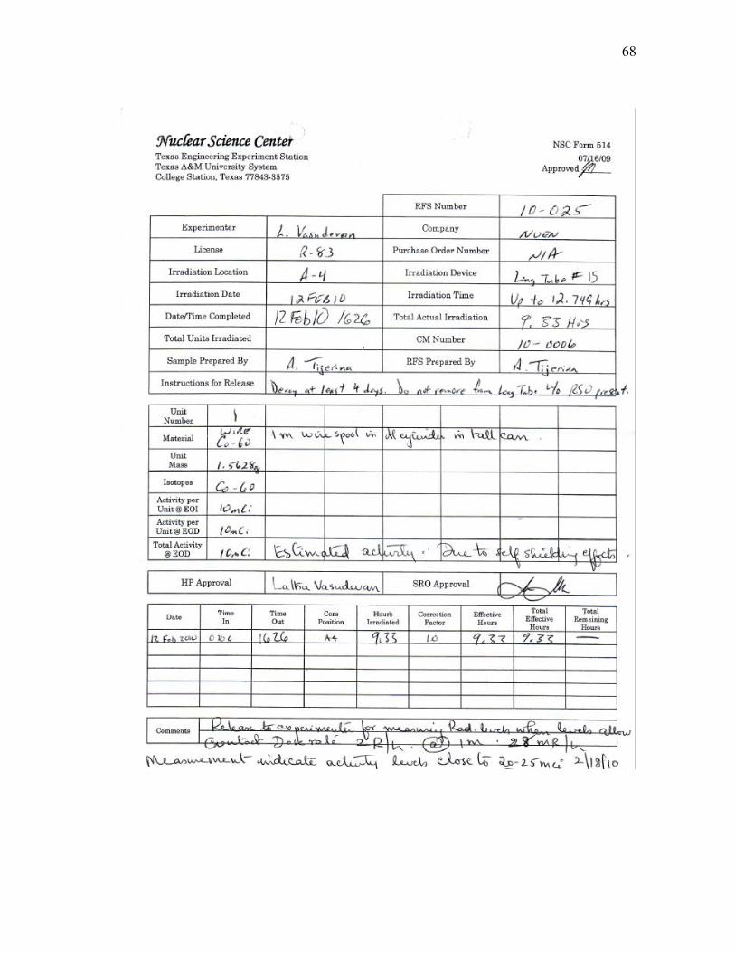
68
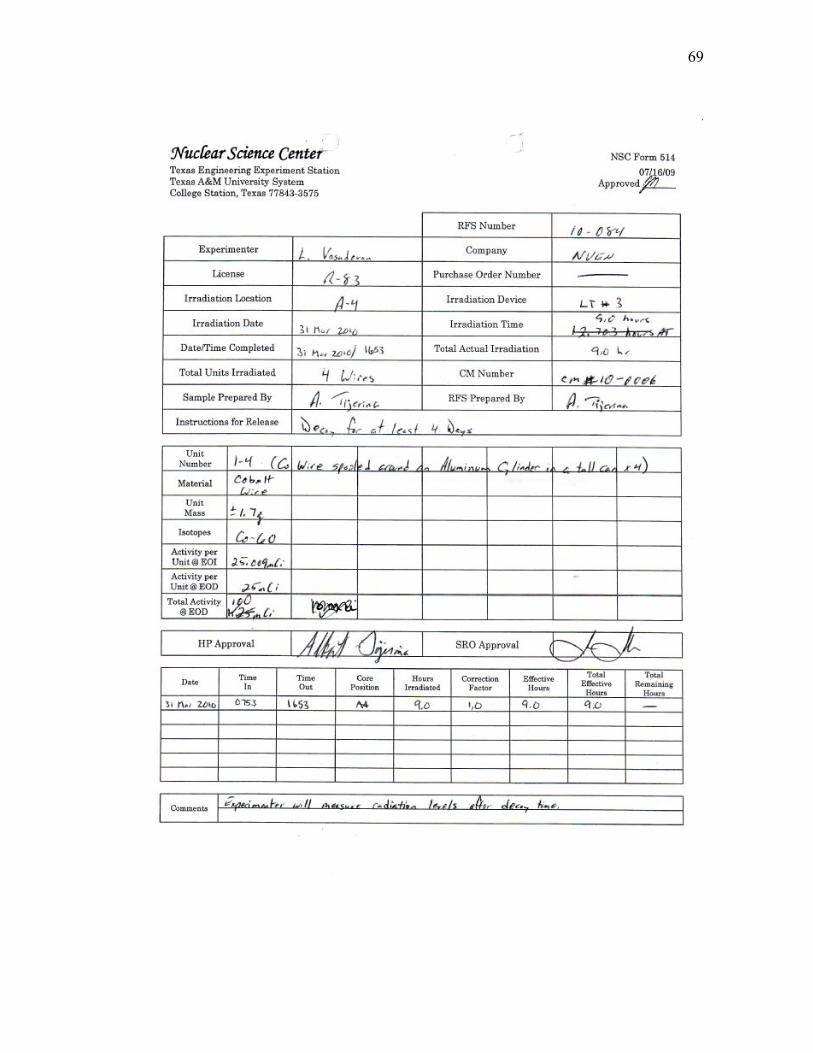
69

70
APPENDIX E
Calibration Glow Curves Generated by Exposing to 0.786 R X-Ray. Figures are Displayed in Order of TLD Number from 1 to 15.
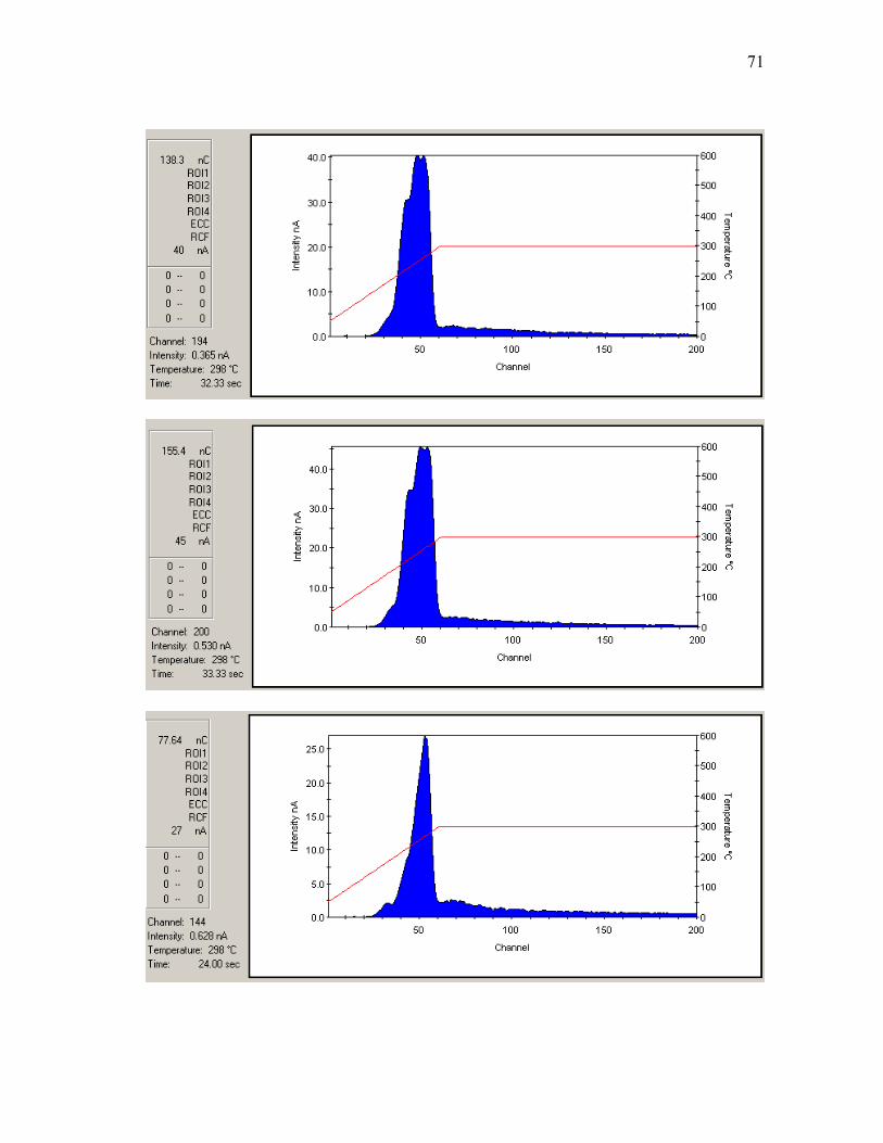
71
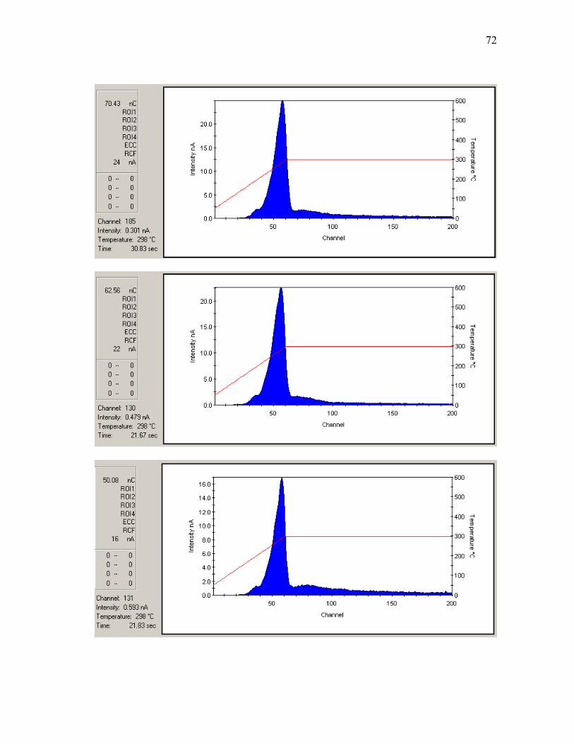
72

73

74

75
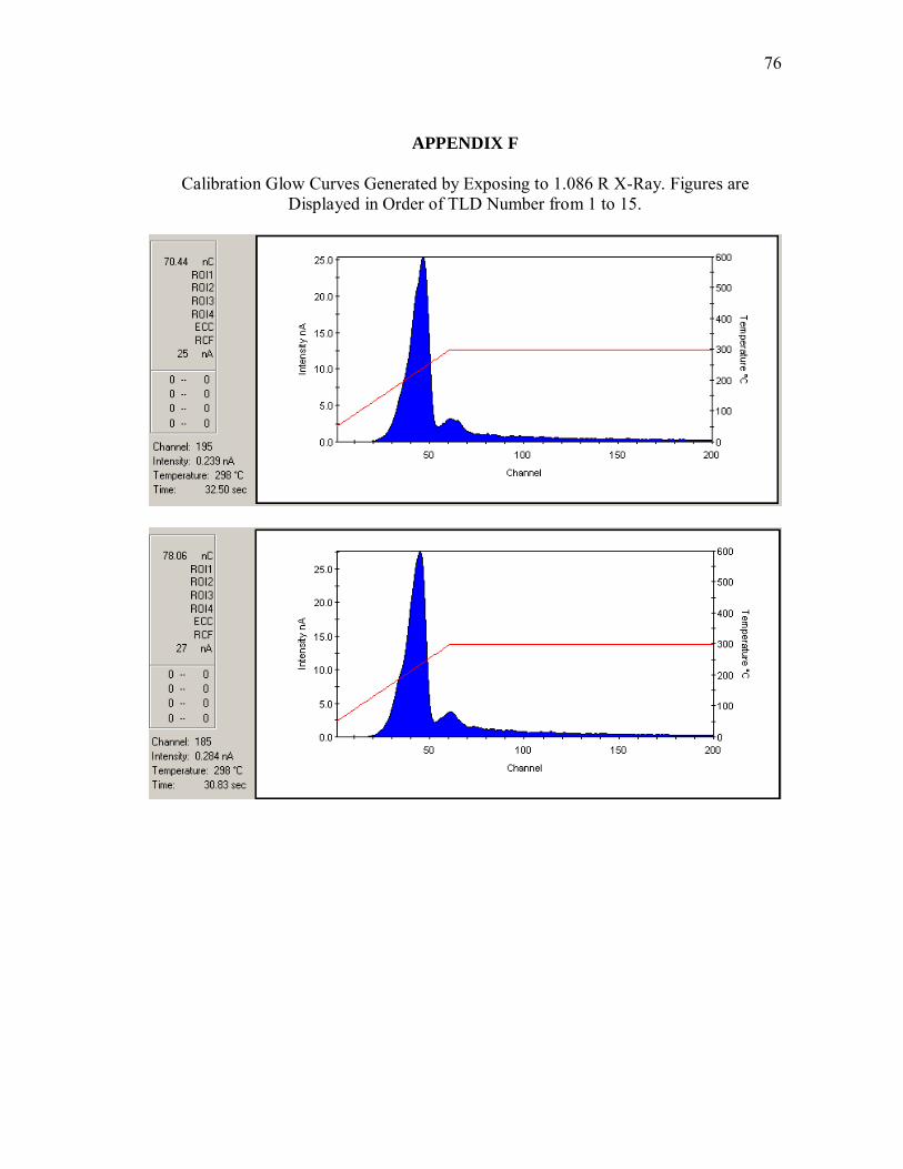
76
APPENDIX F
Calibration Glow Curves Generated by Exposing to 1.086 R X-Ray. Figures are Displayed in Order of TLD Number from 1 to 15.

77

78

79

80
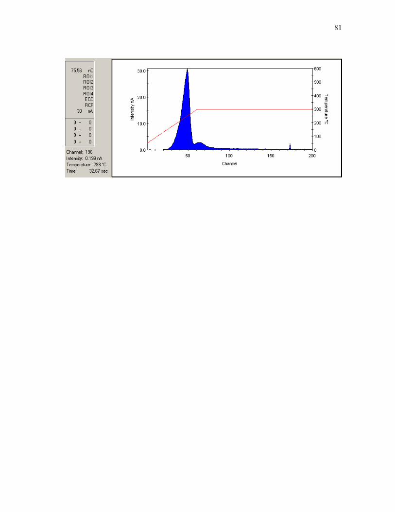
81
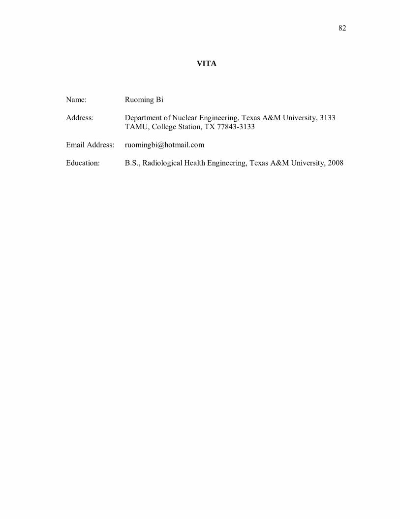
82
VITA
Name: Ruoming Bi
Address: Department of Nuclear Engineering, Texas A&M University, 3133 TAMU, College Station, TX 77843-3133 Email Address: [email protected] Education: B.S., Radiological Health Engineering, Texas A&M University, 2008