cusc - section 14 charging methodologies contents · cusc - section 14 charging methodologies...

CUSC v1.2

of 122 V1.2 – 5th July 2011

CUSC - SECTION 14

CHARGING METHODOLOGIES

CONTENTS

14.1 Introduction

Part I -The Statement of the Connection Charging Methodology 14.2 Principles 14.3 The Calculation of the Basic Annual Connection Charge for an Asset 14.4 Other Charges 14.5 Connection Agreements 14.6 Termination Charges 14.7 Contestability 14.8 Asset Replacement 14.9 Data Requirements 14.10 Applications 14.11 Illustrative Connection Charges 14.12 Examples of Connection Charge Calculations 14.13 Nominally Over Equipped Connection Sites Part 2 -The Statement of the Use of System Charging Methodology

Section 1 – The Statement of the Transmission Use of System Charging Methodology;

14.14 Principles

14.15 Derivation of Transmission Network Use of System Tariff

14.16 Derivation of the Transmission Network Use of System Energy Consumption Tariff and Short Term Capacity Tariffs

14.17 Demand Charges

CUSC v1.2

of 122 V1.2 – 5th July 2011

14.18 Generation Charges

14.19 Data Requirements

14.20 Applications

14.21 Transport Model Example

14.22 Example: Calculation of Zonal Generation Tariff

14.23 Example: Calculation of Zonal Demand Tariff

14.24 Reconciliation of Demand Related Transmission Network Use of System Charges

14.25 Classification of parties for charging purposes

14.26 Transmission Network Use of System Charging Flowcharts

14.27 Example: Determination of The Company’s Forecast for Demand Charge Purposes

14.28 Stability & Predictability of TNUoS tariffs

Section 2 – The Statement of the Balancing Services Use of System Charging Methodology

14.29 Principles

14.30 Calculation of the Daily Balancing Services Use of System charge

14.31 Settlement of BSUoS

14.32 Examples of Balancing Services Use of System (BSUoS) Daily Charge Calculations

CUSC v1.2

of 122 V1.2 – 5th July 2011

CUSC - SECTION 14

CHARGING METHODOLOGIES

14.1 Introduction

14.1.1 This section of the CUSC sets out the statement of the Connection Charging Methodology and the Statement of the Use of System Methodology

CUSC v1.2

of 122 V1.2 – 5th July 2011

CUSC v1.2

of 122 V1.2 – 5th July 2011

Part 1 - The Statement of the Connection Charging

Methodology

14.2 Principles Costs and their Allocation 14.2.1 Connection charges enable The Company to recover, with a reasonable rate of return,

the costs involved in providing the assets that afford connection to the National Electricity Transmission System.

14.2.2 Connection charges relate to the costs of assets installed solely for and only capable

of use by an individual User. These costs may include civil costs, engineering costs, and land clearance and preparation costs associated with the connection assets, but for the avoidance of doubt no land purchase costs will be included..

14.2.3 Connection charges are designed not to discriminate between Users or classes of User.

The methodology is applied to both connections that were in existence at Vesting (30 March 1990) and those that have been provided since.

Connection/Use of System Boundary 14.2.4 The first step in setting charges is to define the boundary between connection assets

and transmission system infrastructure assets. 14.2.5 In general, connection assets are defined as those assets solely required to connect

an individual User to the National Electricity Transmission System, which are not and would not normally be used by any other connected party (i.e. “single user assets”). For the purposes of this Statement, all connection assets at a given location shall together form a connection site.

14.2.6 Connection assets are defined as all those single user assets which:

a) for Double Busbar type connections, are those single user assets connecting the User’s assets and the first transmission licensee owned substation, up to and including the Double Busbar Bay;

b) for teed or mesh connections, are those single user assets from the User’s assets up

to, but not including, the HV disconnector or the equivalent point of isolation;

c) for cable and overhead lines at a transmission voltage, are those single user connection circuits connected at a transmission voltage equal to or less than 2km in length that are not potentially shareable.

14.2.7 Shared assets at a banked connection arrangement will not normally be classed as

connection assets except where both legs of the banking are single user assets under the same Bilateral Connection Agreement.

14.2.8 Where customer choice influences the application of standard rules to the connection

boundary, affected assets will be classed as connection assets. For example, in England & Wales The Company does not normally own busbars below 275kV, where

CUSC v1.2

of 122 V1.2 – 5th July 2011

The Company and the customer agree that The Company will own the busbars at a low voltage substation, the assets at that substation will be classed as connection assets and will not automatically be transferred into infrastructure.

14.2.9 The design of some connection sites may not be compatible with the basic boundary

definitions in 14.2.6 above. In these instances, a connection boundary consistent with the principles described above will be applied.

CUSC v1.2

of 122 V1.2 – 5th July 2011

14.3 The Calculation of the Basic Annual Connection Charge for an Asset Pre and Post Vesting Connections 14.3.1 Post Vesting connection assets are those connection assets that have been

commissioned since 30 March 1990. Pre Vesting connection assets are those that were commissioned on or before the 30 March 1990.

14.3.2 The basic connection charge has two components. A non-capital component, for which

both pre and post vesting assets are treated in the same way and a capital component for which there are slightly different options available for pre and post vesting assets. These are detailed below.

Calculation of the Gross Asset Value (GAV) 14.3.3 The GAV represents the initial total cost of an asset to the transmission licensee. For a

new asset it will be the costs incurred by the transmission licensee in the provision of that asset. Typically, the GAV is made up of the following components:

Construction Costs - Costs of bought in services Engineering - Allocated equipment and direct engineering cost Interest During Construction – Financing cost Liquidated Damages Premiums - Premium required to cover Liquidated Damages if applicable.

Some of these elements may be optional at the User’s request and are a matter of discussion and agreement at the time the connection agreement is entered into.

14.3.4 The GAV of an asset is re-valued each year normally using one of two methods. For

ease of calculation, April is used as the base month.

• In the Modern Equivalent Asset (MEA) revaluation method, the GAV is indexed each year with reference to the prevailing price level for an asset that performs the same function as the original asset;

• In the RPI revaluation method, the original cost of an asset is indexed each year by

the Retail Price Index (RPI) formula set out in paragraph 14.3.6. For Pre Vesting connection assets commissioned on or before 30 March 1990, the original cost is the 1996/97 charging GAV (MEA re-valued from vesting). The original costs of Post Vesting assets are calculated based on historical cost information provided by the transmission licensee’s.

14.3.5 In the MEA revaluation method, the MEA value is based on a typical asset. An MEA

ratio is calculated to account for specific site conditions, as follows:

• The outturn GAV (as calculated in paragraph 14.3.4 above) is re-indexed by RPI to the April of the Financial Year the Charging Date falls within;

• This April figure is compared with the MEA value of the asset in the Financial Year

the Charging Date falls within and a ratio calculated;

• If the asset was commissioned at a Connection Site where, due to specific conditions, the asset cost more than the standard MEA value, the ratio would be greater than 1. For example, if an asset cost 10% more to construct and commission

CUSC v1.2

of 122 V1.2 – 5th July 2011

than the typical asset the MEA ratio would be 1.1. If, however, the asset was found only to cost 90% of the typical MEA value the ratio would be 0.9;

• The MEA ratio is then used in all future revaluations of the asset. The April GAV of

the asset in any year is thus the current MEA value of the asset multiplied by the ratio calculated for the Financial Year the Charging Date falls within.

14.3.6 The RPI revaluation method is as follows:

• The outturn GAV (as calculated in paragraph 14.3.4 above) is re-indexed by RPI to the April of the Financial Year the Charging Date falls within. This April GAV is thus known as the Base Amount;

• The Base Amount GAV is then indexed to the following April by using the RPI

formula used in The Company’s Price Control. April GAVs for subsequent years are found using the same process of indexing by RPI.

i.e. GAVn = GAVn-1 * RPIn

• The RPI calculation for year n is as follows:

[ ][ ] 2-n

1-n n

Index RPI average October toMay Index RPI average October toMay RPI =

Calculation of Net Asset Value 14.3.7 The Net Asset Value (NAV) of each asset for year n, used for charge calculation, is the

average (mid year) depreciated GAV of the asset. The following formula calculates the NAV of an asset, where An is the age of the asset (number of completed charging years old) in year n:

Periodon Depreciati0.5)A(Periodon Depreciati

*GAVNAV n

nn+−

=

14.3.8 In constant price terms an asset with an initial GAV of £1m and a depreciation period

of 40 years will normally have a NAV in the year of its commissioning of £0.9875m (i.e. a reduction of 1.25%) and in its second year of £0.9625m (i.e. a further reduction of 2.5% or one fortieth of the initial GAV). This process will continue with an annual reduction of 2.5% for each year of the asset's life.

Capital Components of the Connection charge for Post Vesting Connection Assets 14.3.9 The standard terms for a connection offer will be:

• 40 year life (with straight line depreciation); • RPI indexation

14.3.10 In addition a number of options exist:

• a capital contribution based on the allocated GAV at the time of commissioning will reduce capital. Typically a capital contribution will include costs to cover the

CUSC v1.2

of 122 V1.2 – 5th July 2011

elements outlined below and charges are calculated as set out in the equations below;

− Construction costs − Engineering costs (Engineering Charge x job hours) − Interest During Construction (IDC) − Return element (6%) − Liquidated Damages Premium (LD) (if applicable) General Formula:

Capital Contribution Charge = (Construction Costs + Engineering Charges) x (1+Return %) + IDC + LD Premium

• MEA revaluation which is combined with a 7.5% rate of return, as against 6% on the

standard RPI basis;

• annual charges based on depreciation periods other than 40 years;

• annuity based charging; • indexation of GAVs based on principles other than MEA revaluation and RPI

indexation. No alternative forms of indexation have been employed to date. 14.3.11 For new connection assets, should a User wish to agree to one or more of the options

detailed above, instead of the standard connection terms, the return elements charged by the transmission licensee may also vary to reflect the re-balancing of risk between the transmission licensee and the User. For example, if Users choose a different indexation method, an appropriate rate of return for such indexation method will be derived.

Capital Components of the Connection charge for Pre Vesting Connection Assets 14.3.12 The basis of connection charges for GB assets commissioned on or before 30 March

1990 is broadly the same as the standard terms for connections made since 30 March 1990. Specifically charges for pre vesting connection assets are based on the following principles:

• The GAV is the 1996/97 charging GAV (MEA re-valued from vesting) subsequently

indexed by the same measure of RPI as used in The Company’s Price Control; • 40 year life (with straight line depreciation); • 6% rate of return

14.3.13 Pre-vesting 1996 MEA GAVs for Users’ connection sites are available from The

Company on request from the Charging Team. Non-Capital Components - Charging for Maintenance and Transmission Running Costs 14.3.14 The non-capital component of the connection charge is divided into two parts, as set

out below. Both of these non-capital elements will normally be identified in the charging appendices of relevant Bilateral Agreements.

CUSC v1.2

of 122 V1.2 – 5th July 2011

Part A: Site Specific Maintenance Charges 14.3.15 This is a maintenance only component that recovers a proportion of the costs and

overheads associated with the maintenance activities conducted on a site-specific basis for connection assets of the transmission licensees.

14.3.16 Site-specific maintenance charges will be calculated each year based on the forecast

total site specific maintenance for NETS divided by the total GAV of the transmission licensees NETS connection assets, to arrive at a percentage of total GAV. For 2010/11 this will be 0.52%. For the avoidance of doubt, there will be no reconciliation of the site-specific maintenance charge.

Part B: Transmission Running Costs 14.3.17 The Transmission Running Cost (TRC) factor is calculated at the beginning of each

price control to reflect the appropriate amount of other Transmission Running Costs (rates, operation, indirect overheads) incurred by the transmission licensees that should be attributed to connection assets.

14.3.18 The TRC factor is calculated by taking a proportion of the forecast Transmission

Running Costs for the transmission licensees (based on operational expenditure figures from the latest price control) that corresponds with the proportion of the transmission licensees’ total connection assets as a function of their total business GAV. This cost factor is therefore expressed as a percentage of an asset's GAV and will be fixed for the entirety of the price control period. For 2010/11 this will be 1.45%.

14.3.19 To illustrate the calculation, the following example uses the average operating

expenditure from the published price control and the connection assets of each transmission licensee expressed as a percentage of their total system GAV to arrive at a GB TRC of 1.45%:

Example:

Connection assets as a percentage of total system GAV for each TO:

Scottish Power Transmission Ltd 15.1%Scottish Hydro Transmission Ltd 8.6%National Grid 12.5%

Published current price control average annual operating expenditure (£m):

Scottish Power Transmission Ltd 29.1Scottish Hydro Transmission Ltd 11.3National Grid 295.2

Total GB Connection GAV = £2.12bn GB TRC Factor = (15.1% x £29.1m + 8.6% x £11.3m + 12.5% x £295.2m) / £2.12bn GB TRC Factor = 1.99% Net GB TRC Factor = Gross GB TRC Factor – Site Specific Maintenance Factor* Net GB TRC Factor = 1.99% - 0.54% = 1.45%

CUSC v1.2

of 122 V1.2 – 5th July 2011

* Note – the Site Specific Maintenance Factor used to calculate the TRC Factor is that which applies for the first year of the price control period or in this example, is the 2007/8 Site Specific Maintenance Factor of 0.54%.

The Basic Annual Connection Charge Formula 14.3.20 The charge for each connection asset in year n can be derived from the general

formula below. This is illustrated more fully by the examples in Appendix 2: Examples of Connection Charge Calculations.

Annual Connection Chargen = Dn (GAVn) + Rn (NAVn) + SSFn (RPIGAVn) + TCn

(GAVn)

Where: For n = year to which charge relates within the Depreciation Period n = year to which charge relates GAVn = GAV for year n re-valued by relevant indexation method RPIGAVn = GAV for year n re-valued by RPI indexation NAVn = NAV for year n based on re-valued GAVn Dn = Depreciation rate as percentage (equal to 1/Depreciation Period)

(typically 1/40 = 2.5% of GAV) Rn = real rate of return for chosen indexation method (6% for RPI

indexation, 7.5% for MEA Indexation) SSFn = Site Specific Factor for year n as a % (equal to the Site

Specific Cost/Total Site GAV) TCn = Transmission Running Cost component for year n (other

Transmission Owner Activity costs). For n = year to which charge relates beyond the Depreciation Period n = year to which charge relates GAVn = GAV for year n re-valued by relevant indexation method RPIGAVn = GAV for year n re-valued by RPI indexation NAVn = 0 Dn = 0 Rn = real rate of return for chosen indexation method (6% for RPI

indexation, 7.5% for MEA Indexation) SSFn = Site Specific Factor for year n as a % (equal to the Site

Specific Cost/Total Site GAV) TCn = Transmission Running cost component for year n (other Transmission

Owner Activity costs). 14.3.21 Note that, for the purposes of deriving asset specific charges for site-specific

maintenance, the RPI re-valued GAV is used. This is to ensure that the exact site charges are recovered from the assets at the site. The site costs are apportioned to the assets on the basis of the ratio of the asset GAV to total Site GAV.

CUSC v1.2

of 122 V1.2 – 5th July 2011

Adjustment for Capital Contributions 14.3.22 If a User chooses to make a 100% capital contribution to The Company towards their

allocation of a connection asset then no capital charges will be payable and hence the connection charges for that asset would be calculated as follows:

Annual Connection Chargen = SSFn (RPIGAVn) + TCn (GAVn)

14.3.23 If a User chooses to make a partial capital contribution to The Company towards their

allocation of a connection asset, for example PCCF = 50%, then the connection charges for that asset would be calculated as follows:

Annual Connection Chargen = Dn (GAVn*PCCF) + Rn (NAVn*PCCF) + SSFn (RPIGAVn) + TCn (GAVn)

PCCF = Partial Capital Contribution Factor

Modification of Connection Assets 14.3.24 Where a modification to an existing connection occurs at the User’s request or due to

developments to the transmission system, their annual connection charges will reflect any additional connection assets that are necessary to meet the User's requirements. Charges will continue to be levied for existing assets that remain in service. Termination charges as described in Chapter 5 below will be charged for any existing connection assets made redundant as a result of the modification.

CUSC v1.2

of 122 V1.2 – 5th July 2011

14.4 Other Charges 14.4.1 In addition to the basic annual connection charges set out above, the User may pay

The Company for certain other costs related to their connection. These will be set out in the Bilateral and Construction Agreements where appropriate and are described below.

One-off Works 14.4.2 To provide or modify a connection, the transmission licensee may be required to carry

out works on the transmission system that, although directly attributable to the connection, may not give rise to additional connection assets. These works are defined as “one-offs”. Liability for one-off charges is established with reference to the principles laid out below:

• Where a cost cannot be capitalised into either a connection or infrastructure asset,

typically a revenue cost

• Where a non-standard incremental cost is incurred as a result of a User's request, irrespective of whether the cost can be capitalised

• Termination Charges associated with the write-off of connection assets at the

connection site.

Consistent with these principles and in accordance with Connection Charging Methodology modification GB ECM-01, which was implemented on 1 December 2005, a one-off charge will be levied for a Category 1 Intertripping Scheme or a Category 3 Intertripping Scheme. A one-off charge will not be levied for a Category 2 Intertripping Scheme or a Category 4 Intertripping Scheme.

14.4.3 The one-off charge is a charge equal to the cost of the works involved, together with a

reasonable return, as shown in 14.4.4 below. 14.4.4 For information, the general formula for the calculation of the one-off charge for works is

outlined below.

One-off Charge = (Construction Costs + Engineering Charges) x (1 + Return %) + IDC + LD Premium

Where: Engineering Charges = “Engineering Charge” x job hours

Return % = 6% IDC = Interest During Construction LD Premium = The Company Liquidated Damages Premium (if applicable)

14.4.5 The calculation of the one-off charge for write-off of assets is outlined below: Write-off Charge = 100% of remaining NAV of redundant assets 14.4.6 One-offs are normally paid on an agreed date, which is usually upon completion of the

works. However, arrangements may be agreed between the transmission licensee and the User to pay the charge over a longer period. If a one-off is paid over a longer period it is termed a Transmission Charge. It is usually a depreciating finance charge or annuity based charge with a rate of return element and may include agreement on a schedule of termination payments if the agreement is terminated before the end of the

CUSC v1.2

of 122 V1.2 – 5th July 2011

annuity period. The charge is usually inflated annually by the same RPI figure that is used to inflate GAVs, though Users can request alternative indexation methods.

Miscellaneous Charges 14.4.7 Other contract specific charges may be payable by the User, these will be set out in the

Bilateral and Construction Agreements where appropriate. Rental sites 14.4.8 Where The Company owns a site that is embedded within a distribution network, the

connection charge to the User is based on the capital costs and overheads but does not include maintenance charges.

Final Metering Scheme (FMS)/Energy Metering Systems 14.4.9 Charges for FMS metering are paid by the registrant of the FMS metering at the

connection site. It is charged on a similar basis as other Connection Assets. The electronic components of the FMS metering have a replacement and depreciation period in line with those advised by the transmission licensees, whilst the non-electronic components normally retain a 40 year replacement and depreciation period (or a User specified depreciation period as appropriate).

CUSC v1.2

of 122 V1.2 – 5th July 2011

14.5 Connection Agreements Indicative Agreement 14.5.1 The standard connection agreement offered by The Company is an indicative price

agreement. From the Charging Date as set out in the User's Bilateral Connection Agreement, the User's initial connection charge is based on a fair and reasonable estimate of the expected costs of the connection.

Outturning the Indicative Agreement 14.5.2 Once the works required to provide a new or modified connection are completed and

the costs finalised, the connection scheme is "outturned". The Company reconciles the monies paid by the User on the indicative charge basis against the charges that would have been payable based on the actual costs incurred in delivering the project together with any relevant interest. This process involves agreeing a new charging GAV (The Base Amount) with the User in line with the elements stated in paragraph 14.3.3 and then calculating connection charges with this GAV.

14.5.3 In addition, for Users that have chosen MEA revaluation their MEA ratios are agreed at

outturn and this ratio is used for MEA revaluation in subsequent years. 14.5.4 In the case of connection asset replacement where there is no initiating User, the

outturn is agreed with the User at the site. Firm Price Agreement 14.5.5 In addition to the options stated in paragraph 14.3.10 above, firm price agreements are

also available. Typically with this option the charges to be incurred, and any indexation, are agreed between The Company and the User and connection charges are not recalculated once outturn costs are known. A typical example of a firm price agreement is:

− Capital Contribution − Firm Price GAV − Running Costs (based on a firm price GAV) − Fixed Schedule of Termination Amounts

14.5.6 When a User selects a firm price agreement some or all of the above elements can be

made firm. Any elements of the agreement that have not been made firm will be charged on an indicative basis in accordance with this statement.

14.5.7 Final Sums and Consents costs are never made firm in a Firm Price Agreement.

Details of both are set out in the Construction Agreement.

CUSC v1.2

of 122 V1.2 – 5th July 2011

Monthly Connection Charges 14.5.8 The connection charge is an annual charge payable monthly. 14.5.9 If the initial Charging Date does not fall within the current Financial Year being charged

for and there are no revisions to charges during the year, the monthly connection charge will equal the annual connection charge divided by twelve.

14.5.10 For the Financial Year in which the Charging Date occurs (as set out in the User's

Bilateral Agreement) or for any Financial Year in which a revision to charges has occurred during the Financial Year, for each complete calendar month from the Charging Date (or effective date of any charge revision) to the end of the Financial Year in which the Charging Date (or charge revision) occurs, the monthly connection charge shall be equal to the annual connection charge divided by twelve.

14.5.11 For each part of a calendar month, the charge will be calculated as one twelfth of the

annual connection charge prorated by the ratio of the number of days from and including the Charging Date to the end of the month that the Charging Date falls in and the number of days in that month.

14.5.12 For example, say the annual connection charge for Financial Year 2010/11 is £1.2m

and the Charging Date falls on the 15th November 2010, the monthly charges for the Financial Year 2010/11 would be as follows:

• November = £1,200,000/12 * (16/30) = £53,333.33 • Dec 10, Jan 11, Feb 11, Mar 11 = £1,200,000/12

= £100,000.00

14.5.13 The above treatment does not apply to elements such as Miscellaneous Charges (as defined in 14.4.7) and Transmission Charges (annuitised one-offs, as defined in 14.4.6). If the Charging Date falls within a Financial Year, then the full annual charge will remain payable and will be spread evenly over the remaining months. This is because these payments are an annuitisation of charges that would normally be paid up-front as one-off payments.

CUSC v1.2

of 122 V1.2 – 5th July 2011

14.6 Termination Charges Charges Liable 14.6.1 Where a User wholly or partially disconnects from the transmission system they will pay

a termination charge. The termination charge will be calculated as follows:

• Where the connection assets are made redundant as a result of the termination or modification of a Bilateral Connection Agreement, the User will be liable to pay an amount equal to the NAV of such assets as at the end of the financial year in which termination or modification occurs, plus:

• The reasonable costs of removing such assets. These costs being inclusive of the

costs of making good the condition of the connection site

• If a connection asset is terminated before the end of a Financial Year, the connection charge for the full year remains payable. Any remaining Use of System Charges (TNUoS and BSUoS) also remain payable

• For assets where it has been determined to replace upon the expiry of the relevant

Replacement Period in accordance with the provisions set out in the CUSC and in respect of which a notice to Disconnect or terminate has been served in respect of the Connection Site at which the assets were located; and due to the timing of the replacement of such assets, no Connection Charges will have become payable in respect of such assets by the User by the date of termination; the termination charges will include the reasonable costs incurred by the transmission licensee in connection with the installation of such assets

• Previous capital contributions paid to The Company will be taken into account

14.6.2 The Calculation of Termination amounts for financial year n is as follows: Termination Chargen = UoSn + Cn + NAVan + R - CC

Where: UoSn = Outstanding Use of System Charge for year (TNUoS and BSUoS) Cn = Outstanding Connection Charge for year NAVan = NAV of Type A assets as at 31 March of financial year n R = Reasonable costs of removal of redundant assets and making good CC = An allowance for previously paid capital contributions

14.6.3 Examples of reasonable costs of removal for terminated assets and making good the

condition of the site include the following:

• If a circuit breaker is terminated as a result of a User leaving a site, this may require modifications to the protection systems.

• If an asset were terminated and its associated civils had been removed to 1m below

ground then the levels would have to be made up. This is a common condition of planning consent.

CUSC v1.2

of 122 V1.2 – 5th July 2011

Repayment on Re-Use of Assets 14.6.4 If any assets in respect of which a termination charge was made to The Company are

re-used at the same site or elsewhere on the system, including use as infrastructure assets, The Company will make a payment to the original terminating User to reflect the fact that the assets are being re-used.

14.6.5 The arrangements for such repayments for re-use of Assets are that The Company will

pay the User a sum equal to the lower of:

i.) the Termination Amount paid in respect of such Assets; or ii.) the NAV attributed to such Assets for charging purposes upon their re-use

less any reasonable costs incurred in respect of the storage of those assets.

14.6.6 The definition of re-use is set out in the CUSC. Where The Company decides to

dispose of a terminated asset where it is capable of re-use, The Company shall pay the User an appropriate proportion of the sale proceeds received.

Valuation of Assets that are re-used as connection assets or existing infrastructure assets re-allocated to connection 14.6.7 If an asset is reused following termination or allocated to connection when it has

previously been allocated to TNUoS, a value needs to be determined for the purposes of connection charges. In both instances the connection charge will be based on the standard formula set out in paragraph 14.3.20. The Gross Asset Value will be based on the original construction costs and indexed by RPI. Where original costs are not known a reasonable value will be agreed between The Company and the User based on similar types of asset in use. The Net Asset Value will be calculated as if the asset had been in continuous service as a connection asset from its original commissioning date taking into account the depreciation period.

14.6.8 Where an asset has been refurbished or updated to bring it back into service a new

value and an appropriate replacement period will be agreed between The Company and the User. This will be based on the value of similar types of asset in service and the costs of the refurbishment.

CUSC v1.2

of 122 V1.2 – 5th July 2011

14.7 Contestability 14.7.1 Some connection activities may be undertaken by the User. The activities are the

provision, or construction, of connection assets, the financing of connection assets and the ongoing maintenance of those assets. While some Users have been keen to see contestability wherever possible, contestability should not prejudice system integrity, security and safety. These concerns have shaped the terms that are offered for contestability in construction and maintenance.

Contestability in Construction 14.7.2 Users have the option to provide (construct) connection assets if they wish. Formal

arrangements for Users exercising this choice are available and further information on User choice in construction can be obtained from the Customer Services Team at:

National Grid House Warwick Technology Park Gallows Hill Warwick CV34 6DA

Telephone 01926 654634

CUSC v1.2

of 122 V1.2 – 5th July 2011

14.8 Asset Replacement 14.8.1 Appendix A of a User's Bilateral Connection Agreement specifies the age (number of

complete charging years old), for charging purposes, of each of the NETS connection assets at the Connection Site for the corresponding Financial Year. Connection charges are calculated on the assumption that the assets will not need to be replaced until the charging age has reached the duration of the asset’s Replacement Period. If a connection asset is to be replaced, The Company will enter into an agreement for the replacement with the User. Where replacement occurs before the original asset’s charging age has reached the duration of its Replacement Period, The Company will continue to charge for the original asset and make no charge to the existing User for the new asset until the original asset’s charging age has reached the duration of its Replacement Period. Where the replacement occurs after the original asset’s charging age has reached the duration of its Replacement Period, The Company will charge on the basis of the original asset until replaced and on the basis of the new asset on completion of the works.

14.8.2 When the original asset’s charging age has reached the duration of its Replacement

Period the User’s charge will be calculated on the then Net Asset Value of the new asset. The new asset begins depreciating for charging purposes upon completion of the asset replacement.

The Basic Annual Connection Charge Formulae are set out in Chapter 2: The Basic Annual Connection Charge Formula.

Asset Replacement that includes a change of Voltage 14.8.3 There are a number of situations where an asset replacement scheme may involve a

change in the voltage level of a User's connection assets. These replacement schemes can take place over a number of years and may involve a long transitory period in which connection assets are operational at both voltage levels.

14.8.4 These situations are inevitably different from case to case and hence further charging

principles will need to be developed over time as more experience is gained. Set out below, are some generic principles. This methodology will be updated as experience develops.

14.8.5 The general principles used to date are to ensure that, in the transitory period of an

asset replacement scheme, the User does not pay for two full transmission voltage substations and that the charges levied reflect the Replacement Period of the original connection assets. In addition, in line with paragraph 14.8.1 above, charges will only be levied for the new assets once the original assets would have required replacement.

14.8.6 For example, a transmission licensee in investing to meet a future Security Standard

need on the main transmission system, may require the asset replacement of an existing 275kV substation with a 400kV substation prior to the expiry of the original assets’ Replacement Period. In this case, The Company will seek to recover the connection asset component via connection charges when the assets replaced were due for asset replacement. Prior to this, the User should not see an increase in charges and therefore the investment costs would be recovered through TNUoS charges.

In addition, if in the interim stage the User has, say, one transformer connected to the

275kV substation and one transformer connected to the 400kV substation, the charge will comprise an appropriate proportion of the HV assets at each site and not the full

CUSC v1.2

of 122 V1.2 – 5th July 2011

costs of the two substations. Note that the treatment described above is only made for transitory asset replacement and not enduring configurations where a User has connection assets connected to two different voltage substations.

CUSC v1.2

of 122 V1.2 – 5th July 2011

14.9 Data Requirements

14.9.1 Under the connection charging methodology no data is required from Users in order to calculate the connection charges payable by the User.

CUSC v1.2

of 122 V1.2 – 5th July 2011

14.10 Applications 14.10.1 Application fees are payable in respect of applications for new connection agreements

and modifications to existing agreements based on the reasonable costs transmission licensees incur in processing these applications. Users can opt to pay a fixed price application fee in respect of their application or pay the actual costs incurred. The fixed price fees for applications are detailed in the Statement of Use of System Charges.

14.10.2 If a User chooses not to pay the fixed fee, the application fee will be based on an

advance of transmission licensees’ Engineering and out-of pocket expenses and will vary according to the size of the scheme and the amount of work involved. Once the associated offer has been signed or lapses, a reconciliation will be undertaken. Where actual expenses exceed the advance, The Company will issue an invoice for the excess. Conversely, where The Company does not use the whole of the advance, the balance will be refunded.

14.10.3 The Company will refund the first application fee paid (the fixed fee or the amount

post-reconciliation) made under the Construction Agreement for new or modified existing agreements. The refund shall be made either on commissioning or against the charges payable in the first three years of the new or modified agreement. The refund will be net of external costs.

14.10.4 The Company will not refund application fees for applications to modify a new

agreement or modified existing agreement at the User’s request before any charges become payable. For example, The Company will not refund an application fee to delay the provision of a new connection if this is made prior to charges becoming payable.

CUSC v1.2

of 122 V1.2 – 5th July 2011

14.11 Illustrative Connection Charges 2010/11 First Year Connection Charges based on the RPI Method (6% rate of return) The following table provides an indication of typical charges for new connection assets. Before using the table, it is important to read through the notes below as they explain the assumptions used in calculating the figures. Calculation of Gross Asset Value (GAV) The GAV figures in the following table were calculated using the following assumptions: • Each asset is new • The GAV includes estimated costs of construction, engineering, Interest During Construction

and Liquidated Damages premiums For details of the Calculation of the Gross Asset Value, see Chapter 2 of this Statement. Calculation of first year connection charge The first year connection charges in the following table were calculated using the following assumptions: • The assets are new • The assets are depreciated over 40 years • The rate of return is assumed to be 6% for RPI indexation • The connection charges include maintenance costs at a rate of 0.52% of the GAV • The connection charges include Transmission Running Costs at a rate of 1.45% of the GAV For details of the Basic Annual Connection Charge Formula, see Chapter 2 of this Statement. Please note that the actual charges will depend on the specific assets at a site. Agreement specific NAVs and GAVs for each User will be made available on request. Notes on Assets The charges for Double and Single Busbar Bays include electrical and civil costs. Transformer cable ratings are based on winter soil conditions. In this example, transformer charges include civil costs of plinth and noise enclosure and estimated transport costs, but not costs of oil dump tank and fire trap moat. Transport costs do not include hiring heavy load sea transportation or roll-on roll-off ships.

CUSC v1.2

of 122 V1.2 – 5th July 2011

£000’s

400kV 275kV 132kV

GAV Charge GAV Charge GAV Charge Double Busbar Bay 2300 239 1890 197 630 65 Single Busbar Bay 1830 190 460 50 Transformer Cables 100m (incl. Cable sealing ends)

120MVA 970 100 310 30 180MVA 1480 150 970 101 320 30 240MVA 1520 158 980 102 355 37 750MVA 1540 160 1135 118 Transformers 45MVA 132/66kV 1060 110 90MVA 132/33kV 102 0 106 120MVA 275/33kV 2110 219 180MVA 275/66kV 2560 266 180MVA 275/132kV 2180 227 240MVA 275/132kV 2630 273 240MVA 400/132kV 3180 340

CUSC v1.2

of 122 V1.2 – 5th July 2011

Connection Examples Example 1

NEW SUPERGRID CONNECTIONSINGLE SWITCH MESH TYPE

A

B

C

A

B

C

LowerVoltage

TransmissionVoltage

SCHEDULE FOR NEW CONNECTION

Ref

A

B

C

2 x 90MVA Transformers

2 x 100m 90MVA Cables

2 x Double BusbarTransformer Bays

Description

212

20

20

252Total

KEY:Existing Transmission Assets (infrastructure)

New connection assets wholly charged tocustomer

Customer Assets

New Transmission Assets (infrastructure)

132/33kV 400/132kV

Description

First YearCharges(£000s)





680

72

130

882Total

CUSC v1.2

of 122 V1.2 – 5th July 2011

Example 2

NEW SUPERGRID CONNECTIONDOUBLE BUSBAR TYPE

A

B

C

A

B

C

DD

TransmissionVoltage

LowerVoltage

KEY:

Customer Assets


Ref

A

B

C

D





Description

382Total

132/33kV 400/132kV

Description


1362Total

Existing Transmission Assets (infrastructure)



130

212

20

20





478

680

74

130


CUSC v1.2

of 122 V1.2 – 5th July 2011

Example 3 EXTENSION OF SINGLE SWITCH MESH

TO FOUR SWITCH MESH(extension to single user site)

A A

TransmissionVoltage

BB

C C

D D

LowerVoltage

KEY:


Customer Assets

Existing connection assets wholly charged toanother user


Existing Transmission Assets (infrastructure)


Ref

A

B

C

D





Description

326Total

132/33kV 400/132kV

Description


1200Total

74

212

20

20





316

680

74

130


Other Users Assets

CUSC v1.2

of 122 V1.2 – 5th July 2011

14.12 Examples of Connection Charge Calculations The following examples of connection charge calculations are intended as general illustrations. Example 1 This example illustrates the method of calculating the first year connection charge for a given asset value. This method of calculation is applicable to indicative price agreements for new connections, utilising the RPI method of charging, and assuming: i) the asset is commissioned on 1 April 2010 ii) there is no inflation from year to year i.e. GAV remains constant iii) the site specific maintenance charge component remains constant throughout the 40

years at 0.52% of GAV iv) the Transmission Running Cost component remains constant throughout the 40 years

at 1.45% of GAV v) the asset is depreciated over 40 years vi) the rate of return charge remains constant at 6% for the 40 year life of the asset vii) the asset is terminated at the end of its 40 year life For the purpose of this example, the asset on which charges are based has a Gross Asset Value of £3,000,000 on 1 April 2010. Charge Calculation

Site Specific Maintenance Charge (0.52% of GAV)

3,000,000 x 0.52% £15,600

Transmission Running Cost (1.45% of GAV)

3,000,000 x 1.45% £43,500

Capital charge (40 year depreciation 2.5% of GAV)

3,000,000 x 2.5% £75,000

Return on mid-year NAV (6%)

2,962,500 x 6% £177,750

TOTAL £311,850 The first year charge of £311,850 would reduce in subsequent years as the NAV of the asset is reduced on a straight-line basis.

This gives the following annual charges over time (assuming no inflation):

Year Charge

1 £311,850 2 £307,350 10 £271,350 40 £136,350

Based on this example, charges of this form would be payable until 31 March 2050.

CUSC v1.2

of 122 V1.2 – 5th July 2011

Example 2 The previous example assumes that the asset is commissioned on 1 April 2010. If it is assumed that the asset is commissioned on 1 July 2010, the first year charge would equal 9/12th of the first year annual connection charge i.e. £233,887.50 This gives the following annual charges over time:

Year Charge

1 £233,887.50 (connection charge for period July to March) 2 £307,350 10 £271,350 40 £136,350

Example 3 In the case of a firm price agreement, there will be two elements in the connection charge, a finance component and a running cost component. These encompass the four elements set out in the examples above. Using exactly the same assumptions as those in example 1 above, the total annual connection charges will be the same as those presented. These charges will not change as a result of the adoption of a different charging methodology by The Company, providing that the connection boundary does not change. Example 4 If a User has chosen a 20-year depreciation period for their Post Vesting connection assets and subsequently remains connected at the site beyond the twentieth year their charges are calculated as follows. For years 21-40 they will pay a connection charge based on the following formula: Annual Connection Chargen = SSFn (RPIGAVn)+ TCn (GAVn) The NAV will be zero and the asset will be fully depreciated so there will be no rate of return or depreciation element to the charge.

CUSC v1.2

of 122 V1.2 – 5th July 2011

14.13 Nominally Over Equipped Connection Sites 14.13.1 This chapter outlines examples of ways in which a connection site can be considered

as having connection assets that exceed the strict, theoretical needs of the individual Users at the connection site. These can be described as:

Historical 14.13.2 This is where the connection assets at the connection site were installed to meet a

requirement of the Users for connection capacity that no longer exists. An example would be where a User, at one time, had a requirement for, say, 270 MW. This would allocate three 240 MVA 400/132kV transformers to the User. Due to reconfiguration of that User’s network only 200 MW is now required from the connection site. The lower requirement would only allocate two transformers, but all the transformers are kept in service. The connection assets will continue to be assigned to the User’s connection, and charged for as connection, until the User makes a Modification Application to reduce the historical requirement. In some cases the Modified requirement will mean that Termination Payments will have to be made on some connection assets.

Early Construction 14.13.3 If a User has a multi-phase project, it may be necessary to install connection assets for

the latter phases at the time of the first phase. These connection assets could be charged from the first phase charging date.

Connection site Specific Technical or Economic Conditions 14.13.4 In circumstances where the transmission licensee has identified a wider requirement

for development of the transmission system, it may elect to install connection assets of greater size and capacity than the practicable minimum scheme required for a particular connection. In these circumstances, however, connection charges for the party seeking connection will normally be based on the level of connection assets consistent with the practicable minimum scheme needed to meet the applicant's requirements.

14.13.5 There may be cases where there are specific conditions such that the practicable

minimum scheme at a site has to be greater than the strict, theoretical interpretation of the standards. In these cases all assets will still be assigned to connection and connection charges levied.

14.13.6 A practicable minimum scheme is considered in terms of the system as a whole and

may include a change in voltage level.

CUSC v1.2

of 122 V1.2 – 5th July 2011

Part 2 - The Statement of the Use of System Charging Methodology

Section 1 – The Statement of the Transmission Use of System

Charging Methodology 14.14 Principles

14.14.1 Transmission Network Use of System charges reflect the cost of installing, operating and maintaining the transmission system for the Transmission Owner (TO) Activity function of the Transmission Businesses of each Transmission Licensee. These activities are undertaken to the standards prescribed by the Transmission Licences, to provide the capability to allow the flow of bulk transfers of power between connection sites and to provide transmission system security.

14.14.2 A Maximum Allowed Revenue (MAR) defined for these activities and those

associated with pre-vesting connections is set by the Authority at the time of the Transmission Owners’ price control review for the succeeding price control period. Transmission Network Use of System Charges are set to recover the Maximum Allowed Revenue as set by the Price Control (where necessary, allowing for any Kt adjustment for under or over recovery in a previous year net of the income recovered through pre-vesting connection charges).

14.14.3 The basis of charging to recover the allowed revenue is the Investment Cost

Related Pricing (ICRP) methodology, which was initially introduced by The Company in 1993/94 for England and Wales. The principles and methods underlying the ICRP methodology were set out in the The Company document "Transmission Use of System Charges Review: Proposed Investment Cost Related Pricing for Use of System (30 June 1992)".

14.14.4 In December 2003, The Company published the Initial Thoughts consultation

for a GB methodology using the England and Wales methodology as the basis for consultation. The Initial Methodologies consultation published by The Company in May 2004 proposed two options for a GB charging methodology with a Final Methodologies consultation published in August 2004 detailing The Company’s response to the Industry with a recommendation for the GB charging methodology. In December 2004, The Company published a Revised Proposals consultation in response to the Authority’s invitation for further review on certain areas in The Company’s recommended GB charging methodology.

14.14.5 In April 2004 The Company introduced a DC Loadflow (DCLF) ICRP based

transport model for the England and Wales charging methodology. The DCLF model has been extended to incorporate Scottish network data with existing England and Wales network data to form the GB network in the model. In April 2005, the GB charging methodology implemented the following proposals:

i.) The application of multi-voltage circuit expansion factors with a forward-

looking Expansion Constant that does not include substation costs in its derivation.

ii.) The application of locational security costs, by applying a multiplier to the

Expansion Constant reflecting the difference in cost incurred on a secure network as opposed to an unsecured network.

CUSC v1.2

of 122 V1.2 – 5th July 2011

iii.) The application of a de-minimus level demand charge of £0/kW for Half

Hourly and £0/kWh for Non Half Hourly metered demand to avoid the introduction of negative demand tariffs.

iv.) The application of 132kV expansion factor on a Transmission Owner

basis reflecting the regional variations in network upgrade plans.

v.) The application of a Transmission Network Use of System Revenue split between generation and demand of 27% and 73% respectively.

vi.) The number of generation zones using the criteria outlined in paragraph

14.15.26 has been determined as 21.

vii.) The number of demand zones has been determined as 14, corresponding to the 14 GSP groups.

14.14.6 The underlying rationale behind Transmission Network Use of System charges

is that efficient economic signals are provided to Users when services are priced to reflect the incremental costs of supplying them. Therefore, charges should reflect the impact that Users of the transmission system at different locations would have on the Transmission Owner's costs, if they were to increase or decrease their use of the respective systems. These costs are primarily defined as the investment costs in the transmission system, maintenance of the transmission system and maintaining a system capable of providing a secure bulk supply of energy.

The Transmission Licence requires The Company to operate the National Electricity Transmission System to specified standards. In addition The Company with other transmission licensees are required to plan and develop the National Electricity Transmission System to meet these standards. These requirements mean that the system must conform to a particular Security Standard and capital investment requirements are largely driven by the need to conform to this standard. It is this obligation, which provides the underlying rationale for the ICRP approach, i.e. for any changes in generation and demand on the system, The Company must ensure that it satisfies the requirements of the Security Standard.

14.14.7 The Security Standard identifies requirements on the capacity of component

sections of the system given the expected generation and demand at each node, such that demand can be met and generators’ Transmission Entry Capacities (TECs) accommodated. The derivation of the incremental investment costs at different points on the system is therefore determined against the requirements of the system at the time of peak demand. The charging methodology therefore recognises this peak element in its rationale.

14.14.8 In setting and reviewing these charges The Company has a number of further

objectives. These are to:

• offer clarity of principles and transparency of the methodology; • inform existing Users and potential new entrants with accurate and stable

cost messages; • charge on the basis of services provided and on the basis of incremental

rather than average costs, and so promote the optimal use of and investment in the transmission system; and

• be implementable within practical cost parameters and time-scales.

CUSC v1.2

of 122 V1.2 – 5th July 2011

14.14.9 Condition C13 of The Company’s Transmission Licence governs the adjustment to Use of System charges for small generators. Under the condition, The Company is required to reduce TNUoS charges paid by eligible small generators by a designated sum, which will be determined by the Authority. The licence condition describes an adjustment to generator charges for eligible plant, and a consequential change to demand charges to recover any shortfall in revenue. The mechanism for recovery will ensure revenue neutrality over the lifetime of its operation although it does allow for effective under or over recovery within any year. For the avoidance of doubt, Condition C13 does not form part of the Use of System Charging Methodology.

14.14.10 The Company will typically calculate TNUoS tariffs annually, publishing final

tariffs in respect of a Financial Year by the end of the preceding January. However The Company may update the tariffs part way through a Financial Year.

CUSC v1.2

of 122 V1.2 – 5th July 2011

14.15 Derivation of the Transmission Network Use of System Tariff

14.15.1 The Transmission Network Use of System (TNUoS) Tariff comprises two separate elements. Firstly, a locationally varying element derived from the DCLF ICRP transport model to reflect the costs of capital investment in, and the maintenance and operation of, a transmission system to provide bulk transport of power to and from different locations. Secondly, a non-locationally varying element related to the provision of residual revenue recovery. The combination of both these elements forms the TNUoS tariff.

14.15.2 For generation TNUoS tariffs the locational element itself is comprised of three

separate components. A wider component reflects the costs of the wider network, and the combination of a local substation and a local circuit component reflect the costs of the local network. Accordingly, the wider tariff represents the combined effect of the wider locational tariff component and the residual element; and the local tariff represents the combination of the two local locational tariff components.

14.15.3 The process for calculating the TNUoS tariff is described below.

The Transport Model

Model Inputs

14.15.4 The DCLF ICRP transport model calculates the marginal costs of investment in

the transmission system which would be required as a consequence of an increase in demand or generation at each connection point or node on the transmission system, based on a study of peak conditions on the transmission system. One measure of the investment costs is in terms of MWkm. This is the concept that ICRP uses to calculate marginal costs of investment. Hence, marginal costs are estimated initially in terms of increases or decreases in units of kilometres (km) of the transmission system for a 1 MW injection to the system.

14.15.5 The transport model requires a set of inputs representative of peak conditions

on the transmission system:

• Nodal generation information • Nodal demand information • Transmission circuits between these nodes • The associated lengths of these routes, the proportion of which is overhead line or

cable and the respective voltage level • The ratio of each of 132kV overhead line, 132kV cable, 275kV overhead line, 275kV

cable and 400kV cable to 400kV overhead line costs to give circuit expansion factors

• 132kV overhead circuit capacity and single/double route construction information is used in the calculation of a generator’s local charge.

• Offshore transmission cost and circuit/substation data • Identification of a reference node

14.15.6 For a given charging year "t", the nodal TEC figure at each node will be based

on the Applicable Value for year "t" in the NETS Seven Year Statement in year "t-1" plus updates to the October of year "t-1". The contracted TECs in the NETS Seven Year Statement include all plant belonging to generators who have a Bilateral Agreement with the TOs. For example, for 2010/11 charges,

CUSC v1.2

of 122 V1.2 – 5th July 2011

the nodal generation data is based on the forecast for 2010/11 in the 2009 NETS Seven Year Statement plus any data included in the quarterly updates in October 2009.

14.15.7 Nodal demand data for the transport model will be based upon the GSP

demand that Users have forecast to occur at the time of National Grid Peak Average Cold Spell (ACS) Demand for year "t" in the April Seven Year Statement for year "t-1" plus updates to the October of year "t-1".

14.15.8 Transmission circuits for charging year "t" will be defined as those with existing

wayleaves for the year "t" with the associated lengths based on the circuit lengths indicated for year "t" in the April NETS Seven Year Statement for year "t-1" plus updates to October of year "t-1". If certain circuit information is not explicitly contained in the NETS Seven Year Statement, The Company will use the best information available.

14.15.9 The circuit lengths included in the transport model are solely those, which

relate to assets defined as 'Use of System' assets.

14.15.10 The transport model employs the use of circuit expansion factors to reflect the difference in cost between (i) cabled routes and overhead line routes, (ii) 132kV and 275kV routes, (iii) 275kV routes and 400kV routes, and (iv), uses 400kV overhead line (i.e. the 400kV overhead line expansion factor is 1). As the transport model expresses cost as marginal km (irrespective of cables or overhead lines), some account needs to be made of the fact that investment in these other types of circuit (specifically 400kV cable, 275kV overhead line, 275kV cable, 132kV overhead line and 132kV cable) is more expensive than for 400kV overhead line. This is done by effectively 'expanding' these more expensive circuits by the relevant circuit expansion factor, thereby producing a larger marginal kilometre to reflect the additional cost of investing in these circuits compared to 400kV overhead line. When calculating the local circuit tariff for a generator, alternative 132kV and offshore expansion factors to those used in the remainder of the tariff calculation are applied to the generator’s local circuits.

14.15.11 A reference node is required as a basis point for the calculation of marginal

costs. It determines the magnitude of the marginal costs but not the relativity. For example, if the reference point were put in the North of Scotland, all nodal generation marginal costs would likely be negative. Conversely, if the reference point were defined at Land's End, all nodal generation marginal costs would be positive. However, the relativity of costs between nodes would stay the same. For information purposes the reference node for 2010/11 is East Claydon 400kV (ECLA40).

Model Outputs

14.15.12 The transport model takes the inputs described above and firstly scales the

nodal generation capacity uniformly such that total national generation (sum of contracted TECs) equals total national ACS Demand. The model then uses a DCLF ICRP transport algorithm to derive the resultant pattern of flows based on the network impedance required to meet the nodal demand using the scaled nodal generation, assuming every circuit has infinite capacity. Then it calculates the resultant total network MWkm, using the relevant circuit expansion factors as appropriate.

CUSC v1.2

of 122 V1.2 – 5th July 2011

14.15.13 Using this baseline network, the model calculates for a given injection of 1MW of generation at each node, with a corresponding 1MW offtake (demand) at the reference node, the increase or decrease in total MWkm of the whole network. Given the assumption of a 1MW injection, for simplicity the marginal costs are expressed solely in km. This gives a marginal km cost for generation at each node (although not that used to calculate generation tariffs which considers local and wider cost components). The marginal km cost for demand at each node equal and opposite to this nodal marginal km for generation and this is used to calculate demand tariffs. Note the marginal km costs can be positive or negative depending on the impact the injection of 1MW of generation has on the total circuit km.

14.15.14 Using a similar methodology, the local and wider marginal km costs used to

determine generation TNUoS tariffs are calculated by injecting 1MW of generation against the node(s) the generator is modelled at and increasing by 1MW the offtake at the reference node. In this model, any circuits identified as local assets to a node will have the local circuit expansion factors are applied in calculating that particular node’s marginal km. Any remaining circuits will have the TO specific wider circuit expansion factors applied.

14.15.15 An example is contained in 14.21 Transport Model Example.

Calculation of local nodal marginal km

14.15.16 In order to ensure assets local to generation are charged in a cost reflective manner, a generation local circuit tariff is calculated. The nodal specific charge provides a financial signal reflecting the security and construction of the infrastructure circuits that connect the node to the transmission system.

14.15.17 Main Interconnected Transmission System (MITS) nodes are defined as:

• Grid Supply Point connections with 2 or more transmission circuits connecting at

the site; or • connections with more than 4 transmission circuits connecting at the site.

14.15.18 Where a Grid Supply Point is defined as a point of supply from the National Electricity Transmission System to network operators or non-embedded customers excluding generator or interconnector load alone. For the avoidance of doubt, generator or interconnector load would be subject to the circuit component of its Local Charge. A transmission circuit is part of the National Electricity Transmission System between two or more circuit-breakers which includes transformers, cables and overhead lines but excludes busbars and generation circuits.

14.15.19 Generators directly connected to a MITS node will have a zero local circuit

tariff.

14.15.20 Generators not connected to a MITS node will have a local circuit tariff derived from the local nodal marginal km for the generation node i.e. the increase or decrease in marginal km along the transmission circuits connecting it to all adjacent MITS nodes (local assets).

Calculation of zonal marginal km

14.15.21 Given the requirement for relatively stable cost messages through the ICRP methodology and administrative simplicity, nodes are assigned to zones. Typically, generation zones will be reviewed at the beginning of each price

CUSC v1.2

of 122 V1.2 – 5th July 2011

control period with another review only undertaken in exceptional circumstances. Any rezoning required during a price control period will be undertaken with the intention of minimal disruption to the established zonal boundaries. The full criteria for determining generation zones are outlined in paragraph 14.15.26. The number of generation zones set for 2010/11 is 20.

14.15.22 Demand zone boundaries have been fixed and relate to the GSP Groups used

for energy market settlement purposes.

14.15.23 The nodal marginal km are amalgamated into zones by weighting them by their relevant generation or demand capacity.

14.15.24 Generators will have a zonal tariff derived from the wider nodal marginal km for

the generation node calculated as the increase or decrease in marginal km along all transmission circuits except those classified as local assets. The zonal marginal km for generation is calculated as:

∑∈

∗=

Gijj

jjj Gen

GenNMkmWNMkm

∑∈

=Gij

jGi WNMkmZMkm

Where

Gi = Generation zone j = Node

NMkm = Wider nodal marginal km from transport model WNMkm = Weighted nodal marginal km ZMkm = Zonal Marginal km Gen = Nodal Generation from the transport model

14.15.25 The zonal marginal km for demand zones are calculated as follows:

∑∈

∗∗−=

Dijj

jjj Dem

DemNMkmWNMkm

1

∑∈

=Dij

jDi WNMkmZMkm

Where Di = Demand zone Dem = Nodal Demand from transport model

14.15.26 A number of criteria are used to determine the definition of the generation zones. Whilst it is the intention of The Company that zones are fixed for the duration of a price control period, it may become necessary in exceptional circumstances to review the boundaries having been set. In both circumstances, the following criteria are used to determine the zonal boundaries:

CUSC v1.2

of 122 V1.2 – 5th July 2011

i.) Zones should contain relevant nodes whose wider marginal costs (as determined

from the output from the transport model, the relevant expansion constant and the locational security factor, see below) are all within +/-£1.00/kW (nominal prices) across the zone. This means a maximum spread of £2.00/kW in nominal prices across the zone.

ii.) The nodes within zones should be geographically and electrically proximate.

iii.) Relevant nodes are considered to be those with generation connected to them as

these are the only ones, which contribute to the calculation of the zonal generation tariff.

14.15.27 The process behind the criteria in 14.15.26 is driven by initially applying the

nodal marginal costs from the DCLF Transport model onto the appropriate areas of a substation line diagram. Generation nodes are grouped into initial zones using the +/- £1.00/kW range. All nodes within each zone are then checked to ensure the geographically and electrically proximate criteria have been met using the substation line diagram. The established zones are inspected to ensure the least number of zones are used with minimal change from previously established zonal boundaries. The zonal boundaries are finally confirmed using the demand nodal costs for guidance.

14.15.28 The zoning criteria are applied to a reasonable range of DCLF ICRP transport

model scenarios, the inputs to which are determined by The Company to create appropriate TNUoS generation zones. The minimum number of zones, which meet the stated criteria, are used. If there is more than one feasible zonal definition of a certain number of zones, The Company determines and uses the one that best reflects the physical system boundaries.

14.15.29 Zones will typically not be reviewed more frequently than once every price

control period to provide some stability. However, in exceptional circumstances, it may be necessary to review zoning more frequently to maintain appropriate, cost reflective, locational cost signals. For example, if a new generator connecting to the transmission system would cause the creation of a new generation zone for that generator alone, it may not be appropriate from a cost reflective perspective to wait until the next price control period to undertake this rezoning. If any such rezoning is required, it will be undertaken against a background of minimal change to existing generation zones and in line with the notification process set out in the Transmission Licence and CUSC.

Deriving the Final Local £/kW Tariff and the Wider £/kW Tariff

14.15.30 The zonal marginal km (ZMkmGi) are converted into costs and hence a tariff by multiplying by the Expansion Constant and the Locational Security Factor (see below). The nodal local marginal km (NLMkmL) are converted into costs and hence a tariff by multiplying by the Expansion Constant and a Local Security Factor.

The Expansion Constant

14.15.31 The expansion constant, expressed in £/MWkm, represents the annuitised value of the transmission infrastructure capital investment required to transport 1 MW over 1 km. Its magnitude is derived from the projected cost of 400kV

CUSC v1.2

of 122 V1.2 – 5th July 2011

overhead line, including an estimate of the cost of capital, to provide for future system expansion.

14.15.32 In the methodology, the expansion constant is used to convert the marginal km

figure derived from the transport model into a £/MW signal. The tariff model performs this calculation, in accordance with 14.15.60 – 14.15.65, and also then calculates the residual element of the overall tariff (to ensure correct revenue recovery in accordance with the price control), in accordance with 14.15.81.

14.15.33 The transmission infrastructure capital costs used in the calculation of the

expansion constant are provided via an externally audited process. They also include information provided from all onshore Transmission Owners (TOs). They are based on historic costs and tender valuations adjusted by a number of indices (e.g. global price of steel, labour, inflation, etc.). The objective of these adjustments is to make the costs reflect current prices, making the tariffs as forward looking as possible. This cost data represents The Company’s best view; however it is considered as commercially sensitive and is therefore treated as confidential. The calculation of the expansion constant also relies on a significant amount of transmission asset information, much of which is provided in the Seven Year Statement.

14.15.34 For each circuit type and voltage used onshore, an individual calculation is

carried out to establish a £/MWkm figure, normalised against the 400KV overhead line (OHL) figure, these provide the basis of the onshore circuit expansion factors discussed in 14.15.42 – 14.15.47. In order to simplify the calculation a unity power factor is assumed, converting £/MVAkm to £/MWkm. This reflects that the fact tariffs and charges are based on real power.

14.15.35 The table below shows the first stage in calculating the onshore expansion

constant. A range of overhead line types is used and the types are weighted by recent usage on the transmission system. This is a simplified calculation for 400kV OHL using example data:

400kV OHL expansion constant calculation MW Type £(000)/k Circuit km* £/MWkm Weight A B C D E = C/A F=E*D 6500 La 700 500 107.69 53846 6500 Lb 780 0 120.00 0 3500 La/b 600 200 171.43 34286 3600 Lc 400 300 111.11 33333 4000 Lc/a 450 1100 112.50 123750 5000 Ld 500 300 100.00 30000 5400 Ld/a 550 100 101.85 10185 Sum 2500 (G) 285400 (H)

Weighted Average (J= H/G):

114.160 (J)

*These are circuit km of types that have been provided in the previous 10 years. If no information is available for a particular category the best forecast will be used.

CUSC v1.2

of 122 V1.2 – 5th July 2011

14.15.36 The weighted average £/MWkm (J in the example above) is then converted in to an annual figure by multiplying it by an annuity factor. The formula used to calculate of the annuity factor is shown below:

( )( )⎥⎦

⎤⎢⎣

⎡ +−=

−

WACCWACC

torAnnuityfacAssetLife11

1

14.15.37 The Weighted Average Cost of Capital (WACC) and asset life are established

at the start of a price control and remain constant throughout a price control period. The WACC used in the calculation of the annuity factor is the The Company regulated rate of return, this assumes that it will be reasonably representative of all licensees. The asset life used in the calculation is 50 years; the appropriateness of this is reviewed when the annuity factor is recalculated at the start of a price control period. These assumptions provide a current annuity factor of 0.066.

14.15.38 The final step in calculating the expansion constant is to add a share of the

annual transmission overheads (maintenance, rates etc). This is done by multiplying the average weighted cost (J) by an ‘overhead factor’. The ‘overhead factor’ represents the total business overhead in any year divided by the total Gross Asset Value (GAV) of the transmission system. This is recalculated at the start of each price control period. The overhead factor used in the calculation of the expansion constant for 2009/10 is 1.8%. The overhead and annuitised costs are then added to give the expansion constant.

14.15.39 Using the previous example, the final steps in establishing the expansion

constant are demonstrated below:

400kV OHL expansion constant calculation Ave £/MWkm

OHL 114.160

Annuitised 7.535

Overhead 2.055

Final 9.589

14.15.40 This process is carried out for each voltage onshore, along with other adjustments to take account of upgrade options, see 14.15.45, and normalised against the 400KV overhead line cost (the expansion constant) the resulting ratios provide the basis of the onshore expansion factors. The process used to derive circuit expansion factors for Offshore Transmission Owner networks is described in 14.15.50.

14.15.41 This process of calculating the incremental cost of capacity for a 400kV OHL,

along with calculating the onshore expansion factors is carried out for the first year of the price control and is increased by inflation, RPI, (May–October average increase, as defined in The Company’s Transmission Licence) each subsequent year of the price control period. The expansion constant for 2010/11 is 10.633.

Onshore Wider Circuit Expansion Factors 14.15.42 Base onshore expansion factors are calculated by deriving individual

expansion constants for the various types of circuit, following the same principles used to calculate the 400kV overhead line expansion constant. The

CUSC v1.2

of 122 V1.2 – 5th July 2011

factors are then derived by dividing the calculated expansion constant by the 400kV overhead line expansion constant. The factors will be fixed for each respective price control period.

14.15.43 In calculating the onshore cable factors, the forecast costs are weighted

equally between urban and rural installation, and direct burial has been assumed. The operating costs for cable are aligned with those for overhead line. An allowance for overhead costs has also been included in the calculations.

14.15.44 The 132kV onshore circuit expansion factor is applied on a TO basis. This is to

reflect the regional variation of plans to rebuild circuits at a lower voltage capacity to 400kV. The 132kV cable and line factor is calculated on the proportion of 132kV circuits likely to be uprated to 400kV. The 132kV expansion factor is then calculated by weighting the 132kV cable and overhead line costs with the relevant 400kV expansion factor, based on the proportion of 132kV circuitry to be uprated to 400kV. For example, in the TO areas of National Grid and Scottish Power where there are no plans to uprate any 132kV circuits, the full cable and overhead line costs of 132kV circuit are reflected in the 132kV expansion factor calculation.

14.15.45 The 275kV onshore circuit expansion factor is applied on a GB basis and

includes a weighting of 83% of the relevant 400kV cable and overhead line factor. This is to reflect the averaged proportion of circuits across all three Transmission Licensees which are likely to be uprated from 275kV to 400kV across GB within a price control period.

14.15.46 The 400kV onshore circuit expansion factor is applied on a GB basis and

reflects the full costs for 400kV cable and overhead lines.

14.15.47 The TO specific onshore circuit expansion factors calculated for 2008/9 (and rounded to 2 decimal places) are:

Scottish Hydro Region 400kV cable factor: 22.39 275kV cable factor: 22.39 132kV cable factor: 27.79 400kV line factor: 1.00 275kV line factor: 1.14 132kV line factor: 2.24 Scottish Power & National Grid Regions 400kV cable factor: 22.39 275kV cable factor: 22.39 132kV cable factor: 30.22 400kV line factor: 1.00 275kV line factor: 1.14 132kV line factor: 2.80

Onshore Local Circuit Expansion Factors 14.15.48 The local onshore circuit tariff is calculated using local onshore circuit

expansion factors. These expansion factors are calculated using the same methodology as the onshore wider expansion factor but without taking into account the proportion of circuit kms that are planned to be uprated.

CUSC v1.2

of 122 V1.2 – 5th July 2011

14.15.49 In addition, the 132kV onshore overhead line circuit expansion factor is sub

divided into four more specific expansion factors. This is based upon maximum (winter) circuit continuous rating (MVA) and route construction whether double or single circuit.

400kV cable factor: 22.39 275kV cable factor: 22.39 132kV cable factor: 30.22 400kV line factor: 1.00 275kV line factor: 1.14

132kV line factor (single; <200MVA): 10.00 132kV line factor (double; <200MVA): 8.32 132kV line factor (single; >=200MVA): 7.13 132kV line factor (double; >=200MVA): 4.42

Offshore Circuit Expansion Factors

14.15.50 Offshore expansion factors (£/MWkm) are derived from information provided by Offshore Transmission Owners for each offshore circuit. Offshore expansion factors are Offshore Transmission Owner and circuit specific. Each Offshore Transmission Owner will periodically provide, via the STC, information to derive an annual circuit revenue requirement. The offshore circuit revenue shall include revenues associated with the Offshore Transmission Owner’s reactive compensation equipment, harmonic filtering equipment, asset spares and HVDC converter stations.

14.15.51 In the first year of connection, the offshore circuit expansion factor would be

calculated as follows:

ConstantExpansionOHL400kVOnshoreCircRatL

CRevOFTO1÷

×

Where: CRevOFTO1 = The offshore circuit revenue in £ for Year 1 L = The total circuit length in km of the offshore circuit CircRat = The continuous rating of the offshore circuit 14.15.52 In all subsequent years, the offshore circuit expansion factor would be

calculated as follows:

ConstantExpansionOHL400kVOnshoreCircRatL

AvCRevOFTO÷

×

Where: AvCRevOFTO = The annual offshore circuit revenue averaged over the

remaining years of the onshore National Electricity Transmission System Operator (NETSO) price control

L = The total circuit length in km of the offshore circuit CircRat = The continuous rating of the offshore circuit 14.15.53 Prevailing OFFSHORE TRANSMISSION OWNER specific expansion factors

will be published in this statement. These shall be re-calculated at the start of each price control when the onshore expansion constants are revisited.

CUSC v1.2

of 122 V1.2 – 5th July 2011

The Locational Onshore Security Factor

14.15.54 The locational onshore security factor is derived by running a secure DCLF ICRP transport study based on the same market background as used in the DCLF ICRP transport model. This calculates the nodal marginal costs where peak demand can be met despite the Security and Quality of Supply Standard contingencies (simulating single and double circuit faults) on the network. Essentially the calculation of secured nodal marginal costs is identical to the process outlined above except that the secure DCLF study additionally calculates a nodal marginal cost taking into account the requirement to be secure against a set of worse case contingencies in terms of maximum flow for each circuit.

14.15.55 The secured nodal cost differential is compared to that produced by the DCLF

ICRP transport model and the resultant ratio of the two determines the locational security factor using the Least Squares Fit method. Further information may be obtained from the charging website1.

14.15.56 The locational onshore security factor derived for 2010/11 is 1.8 and is based

on an average from a number of studies conducted by The Company to account for future network developments. The security factor is reviewed for each price control period and fixed for the duration.

Local Security Factors

14.15.57 Local onshore security factors are generator specific and are applied to a generators local onshore circuits. If the loss of any one of the local circuits prevents the export of power from the generator to the MITS then a local security factor of 1.0 is applied. For generation with circuit redundancy, a local security factor is applied that is equal to the locational security factor, currently 1.8.

14.15.58 A specific offshore local security factor (LocalSF) will be calculated for each

offshore connection using the following methodology:

∑=

kkGen

yortCapacitNetworkExpLocalSF

Where: NetworkExportCapacity = the total export capacity of the network k = the generation connected to the offshore network

14.15.59 The offshore security factor for single circuits with a single cable will be 1.0 and

for multiple circuit connections will be capped at the locational onshore security factor, derived as 1.8 for 2010/11.

Initial Transport Tariff

14.15.60 First an Initial Transport Tariff (ITT) must be calculated. For Generation the zonal marginal km (ZMkm) are simply multiplied by the expansion constant and the locational security factor to give the initial transport tariff:

1 http://www.nationalgrid.com/uk/Electricity/Charges/

CUSC v1.2

of 122 V1.2 – 5th July 2011

GiGi ITTLSFECZMkm =××

Where

ZMkmGi = Zonal Marginal km for each generation zone EC = Expansion Constant

LSF = Locational Security Factor ITTGi = Initial Transport Tariff (£/MW) for each generation zone

14.15.61 Similarly, for demand the zonal marginal km (ZMkm) are simply multiplied by the expansion constant and the locational security factor to give the initial transport tariff:

DiDi ITTLSFECZMkm =××

Where ZMkmDi = Zonal Marginal km for each demand zone EC = Expansion Constant

LSF = Locational Security Factor ITTDi = Initial Transport Tariff (£/MW) for each demand zone

14.15.62 The next step is to multiply these initial transport tariffs by the expected metered triad demand and generation capacity to gain an estimate of the initial revenue recovery. Both of these latter parameters are based on forecasts provided by Users and are confidential.

( )∑=

=×21

1GiGGiGi ITRRGITT and ( )∑

=

=×14

1DiDDiDi ITRRDITT

Where ITRRG = Initial Transport Revenue Recovery for generation

GGi = Total forecast Generation for each generation zone (based on confidential User forecasts)

ITRRD = Initial Transport Revenue Recovery for demand DDi = Total forecast Metered Triad Demand for each demand zone

(based on confidential User forecasts)

14.15.63 The next stage is to correct the Initial Transport Revenue Recovery figures above such that the 'correct' split of revenue between generation and demand is obtained. This has been determined to be 27:73 by the Authority for generation and demand respectively. In order to achieve the 'correct' generation/demand revenue split, a single additive constant C is calculated which is then added to the total zonal marginal km, both for generation and demand as below:

( )[ ]∑=

=×××+21

1GiGGiGi CTRRGLSFECCZMkm

( )[ ] DDi

DiDi CTRRDLSFECCZMkm =×××−∑=

14

1

CUSC v1.2

of 122 V1.2 – 5th July 2011

Where C is set such that

( )DGD CTRRCTRRpCTRR += Where CTRR = "Generation / Demand split" corrected transport revenue recovery

p = Proportion of revenue to be recovered from demand C = "Generation /Demand split" Correction constant (in km)

14.15.64 The above equations deliver corrected (£/MW) transport tariffs (CTT).

( ) GiGi CTTLSFECCZMkm =××+

( ) DiDi CTTLSFECCZMkm =××−

So that

( ) GGi

GiGi CTRRGCTT =×∑=

21

1 and ( )∑

=

=×14

1DiDDiDi CTRRDCTT

Deriving the Final Local Tariff (£/kW)

Local Circuit Tariff

14.15.65 Generation with a local circuit tariff is calculated by multiplying the nodal

marginal km along the local circuit by the expansion constant and the relevant local security factor (whether onshore or offshore) and summing across local circuits to give the local circuit tariff:

Gik

kL

Gj CLTLocalSFECNLMkm

=××

∑ 1000

Where

k = Local circuit k for generator NLMkmGj

L = Nodal marginal km along local circuit k using local circuit expansion factor.

EC = Expansion Constant LocalSFk = Local Security Factor for circuit k

CLTGi = Circuit Local Tariff (£/kW)

Onshore Local Substation Tariff

14.15.66 All chargeable generation is subject to the local substation tariff component which is determined by assessing the generation substation type which is the substation at the connection charging boundary, against three cost determining factors:

CUSC v1.2

of 122 V1.2 – 5th July 2011

(a) HV connection voltage – the voltage at the boundary between the User’s

connection assets and the transmission system; (b) Sum of TEC at the generation substation – the combined TEC of all generation at

the connecting substation; and (c) The level of redundancy at the generation substation – single busbar / single

switch mesh connections are examples of no redundancy connections, whereas examples of connections with redundancy include double busbar and mesh sub station designs.

14.15.67 Using the above factors, the corresponding £/kW tariffs (quoted to 3dp) that will

be applied during 2010/11 are:

Substation Voltage (a) Substation Rating (b)

Connection Type (c) 132kV 275kV 400kV

<1320MW No redundancy 0.133 0.081 0.065 <1320MW Redundancy 0.301 0.192 0.155 >=1320MW No redundancy n/a 0.257 0.208 >=1320MW Redundancy n/a 0.417 0.336

14.15.68 The process for calculating Local Substation Tariffs will be carried out for the

first year of the price control and will subsequently be indexed by RPI for each subsequent year of the price control period.

14.15.69 The effective Local Tariff (£/kW) is calculated as the sum of the circuit and

substation onshore and/or offshore components: GiGiGi SLTCLTELT +=

Where ELTGi = Effective Local Tariff (£/kW) SLTGi = Substation Local Tariff (£/kW) 14.15.70 Where tariffs do not change mid way through a charging year, final local tariffs

will be the same as the effective tariffs: ELTGi = LTGi Where LTGi = Final Local Tariff (£/kW) 14.15.71 Where tariffs are changed part way through the year, the final tariffs will be

calculated by scaling the effective tariffs to reflect that the tariffs are only applicable for part of the year and parties may have already incurred TNUoS liability.

∑

∑

=

=

×

⎟⎠

⎞⎜⎝

⎛−××

= 21

1

21

112

GiGi

GiGi

GiGi

Gi

Gb

FLLGELTLT

Where: b = number of months the revised tariff is applicable for FLL = Forecast local liability incurred over the period that the original tariff is applicable for

CUSC v1.2

of 122 V1.2 – 5th July 2011

14.15.72 For the purposes of charge setting, the total local charge revenue is calculated by:

j

GijG*LT LCRR GiG ∑

=

=

Where LCRRG = Local Charge Revenue Recovery Gj = Forecast chargeable Generation or Transmission Entry Capacity

in kW (as applicable) for each generator (based on confidential information received from Users)

Offshore substation local tariff

14.15.73 All offshore chargeable generation is subject to an offshore substation tariff. The offshore substation tariff shall be the sum of transformer, switchgear and platform components.

14.15.74 Each tariff component, expressed in £/kW, shall be the ratio of the Offshore

Transmission Owner revenue (£) and rating associated with the transformers, switchgear or platform (kW) at each offshore substation. The Offshore Transmission Owner revenue of each tariff component shall include that associated with asset spares. In the case of the platform component, the relevant rating shall be the lower of the transformer or switchgear ratings. As with the offshore circuit expansion factors, the Offshore Transmission Owner revenue associated with each tariff component shall be averaged over the remaining years of the NETSO price control.

14.15.75 Offshore Transmission Owner revenue associated with interest during

construction and project development overheads will be attributed to the relevant asset category with which it is associated. If these or any other costs included in the Offshore Transmission Owner revenue are not readily attributable to a given asset category, they will be pro-rated across the various asset categories based on their relative cost.

14.15.76 For 2010/11 a discount of £0.345590/kW shall be provided to the offshore

substation tariff to reflect the average cost of civil engineering for onshore substations. This will be inflated by RPI each year and reviewed every price control period.

14.15.77 Offshore substation tariffs shall be inflated by RPI each year and reviewed

every price control period.

14.15.78 The revenue from the offshore substation local tariff is calculated by:

∑ ∑ ⎟⎠

⎞⎜⎝

⎛×=

ssubstationoffshoreAll k

kk GenSLTSLTR

Where: SLTk = the offshore substation tariff for substation k Genk = the generation connected to offshore substation k The Residual Tariff

14.15.79 The total revenue to be recovered through TNUoS charges is determined each year with reference to the Transmission Licensees’ Price Control formulas less the costs expected to be recovered through Pre-Vesting connection charges.

CUSC v1.2

of 122 V1.2 – 5th July 2011

Hence in any given year t, a target revenue figure for TNUoS charges (TRRt) is set after adjusting for any under or over recovery for and including, the small generators discount is as follows:

1−−−= tttt SGPVCRTRR

Where TRRt = TNUoS Revenue Recovery target for year t Rt = Forecast Revenue allowed under The Company’s RPI-X Price Control

Formula for year t (this term includes a number of adjustments, including for over/under recovery from the previous year). For further information, refer to Special Condition D2 of The Company’s Transmission Licence.

PVCt = Forecast Revenue from Pre-Vesting connection charges for year t SGt-1 = The proportion of the under/over recovery included within Rt which relates

to the operation of statement C13 of the The Company Transmission Licence. Should the operation of statement C13 result in an under recovery in year t – 1, the SG figure will be positive and vice versa for an over recovery.

14.15.80 In normal circumstances, the revenue forecast to be recovered from the

corrected transport tariffs will not equate to the total revenue target. This is due to a number of factors. For example, the transport model assumes, for simplicity, smooth incremental transmission investments can be made. In reality, transmission investment can only be made in discrete 'lumps'. The transmission system has been planned and developed over a long period of time. Forecasts and assessments used for planning purposes will not have been borne out precisely by events and therefore some distinction between an optimal system for one year and the actual system can be expected.

14.15.81 As a result of the factors above, in order to ensure adequate revenue recovery, a constant non-locational Residual Tariff for generation and demand is calculated, which includes infrastructure substation asset costs. It is added to the corrected transport tariffs so that the correct generation / demand revenue split is maintained and the total revenue recovery is achieved.

( )

∑=

−×= 14

1DiDi

DD

D

CTRRTRRpRT

( )[ ]

∑=

−−×−= 21

1

1

GiGi

GGG

G

LCRRCTRRTRRpRT

Where RT = Residual Tariff (£/MW) p = Proportion of revenue to be recovered from demand Final £/kW Tariff

14.15.82 The effective Transmission Network Use of System tariff (TNUoS) can now be calculated as the sum of the corrected transport wider tariff, the non-locational residual tariff and the local tariff:

GiGGi

Gi LTRTCTT

ET ++

=1000

and 1000

DDiDi

RTCTTET

+=

CUSC v1.2

of 122 V1.2 – 5th July 2011

Where ET = Effective TNUoS Tariff expressed in £/kW

14.15.83 Where tariffs do not change mid way through a charging year, final demand and generation tariffs will be the same as the effective tariffs.

GiGi ETFT = and DiDi ETFT = 14.15.84 Where tariffs are changed part way through the year, the final tariffs will be

calculated by scaling the effective tariffs to reflect that the tariffs are only applicable for part of the year and parties may have already incurred TNUoS liability.

∑

∑

=

=

×

⎟⎠

⎞⎜⎝

⎛−××

= 21

1

21

112

GiGi

GiGi

GiGi

Gi

Gb

FLGETFT and

∑

∑

=

=

×

⎟⎠

⎞⎜⎝

⎛−××

= 14

1

14

112

DiDi

DiDi

DiDi

Di

Db

FLDETFT

Where: b = number of months the revised tariff is applicable for FL = Forecast liability incurred over the period that the original tariff is applicable for

14.15.85 If the final demand TNUoS Tariff results in a negative number then this is

collared to £0/kW with the resultant non-recovered revenue smeared over the remaining demand zones:

If 0<DiFT , then i = 1 to z

Therefore, ( )

∑

∑

+=

=

×= 14

1

1

ziDi

z

iDiDi

D

D

DFTNRRT

Therefore the revised Final Tariff for the demand zones with positive Final tariffs is given

by:

For i= 1 to z: 0=DiRFT

For i=z+1 to 14: DDiDi NRRTFTRFT +=

Where NRRTD = Non Recovered Revenue Tariff (£/kW) RFTDi = Revised Final Tariff (£/kW)

14.15.86 The tariffs applicable for any particular year are detailed in The Company's

Statement of Use of System Charges, which is available from the Charging website. Archived tariff information may also be obtained from the Charging website.

14.15.87 The zonal maps referenced in The Company's Statement of Use of System

Charges and available on the Charging website contain detailed information for the charging year in question of which Grid Supply Points fall into which TNUoS zones.

CUSC v1.2

of 122 V1.2 – 5th July 2011

14.15.88 New Grid Supply Points will be classified into zones on the following basis:

• For demand zones, according to the GSP Group to which the Grid Supply Point is

allocated for energy market settlement purposes. • For generation zones, with reference to the geographic proximity to existing zones

and, where close to a boundary between existing zones, with reference to the marginal costs arising from transport model studies. The GSP will then be allocated to the zone, which contains the most similar marginal costs.

14.15.89 The Company has available, upon request, the DCLF ICRP transport model,

tariff model template and data necessary to run the model, consisting of nodal values of generation and demand connection points to the NETS. The model and data will enable the basic nodal charges to be determined and will also allow sensitivity analysis concerning alternative developments of generation and demand to be undertaken. The model is available from the Charging Team and whilst it is free of charge, it is provided under licence to restrict its distribution and commercial use.

14.15.90 The Company will be pleased to run specific sensitivity studies for Users under

a separate study contract in line with the fees set out in the Statement of Use of System Charges. Please contact the Charging Team.

14.15.91 The factors which will affect the level of TNUoS charges from year to year

include the forecast level of peak demand on the system, the Price Control formula (including the effect of any under/over recovery from the previous year), the expansion constant, the locational security factor, changes in the transmission network and changes in the pattern of generation capacity and demand.

14.15.92 In accordance with Standard Licence Condition C13, generation directly

connected to the NETS 132kV transmission network which would normally be subject to generation TNUoS charges but would not, on the basis of generating capacity, be liable for charges if it were connected to a licensed distribution network qualifies for a reduction in transmission charges by a designated sum, determined by the Authority. Any shortfall in recovery will result in a unit amount increase in demand charges to compensate for the deficit. Further information is provided in the Statement of the Use of System Charges.

Stability & Predictability of TNUoS tariffs

14.15.93 A number of provisions are included within the methodology to promote the stability and predictability of TNUoS tariffs. These are described in 14.28.

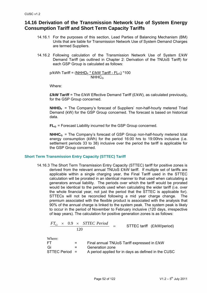
CUSC v1.2

of 122 V1.2 – 5th July 2011

14.16 Derivation of the Transmission Network Use of System Energy Consumption Tariff and Short Term Capacity Tariffs

14.16.1 For the purposes of this section, Lead Parties of Balancing Mechanism (BM) Units that are liable for Transmission Network Use of System Demand Charges are termed Suppliers.

14.16.2 Following calculation of the Transmission Network Use of System £/kW

Demand Tariff (as outlined in Chapter 2: Derivation of the TNUoS Tariff) for each GSP Group is calculated as follows:

p/kWh Tariff = (NHHDF * £/kW Tariff - FLG) *100

NHHCG

Where:

£/kW Tariff = The £/kW Effective Demand Tariff (£/kW), as calculated previously,

for the GSP Group concerned.

NHHDF = The Company’s forecast of Suppliers’ non-half-hourly metered Triad Demand (kW) for the GSP Group concerned. The forecast is based on historical data. FLG = Forecast Liability incurred for the GSP Group concerned. NHHCG = The Company’s forecast of GSP Group non-half-hourly metered total energy consumption (kWh) for the period 16:00 hrs to 19:00hrs inclusive (i.e. settlement periods 33 to 38) inclusive over the period the tariff is applicable for the GSP Group concerned.

Short Term Transmission Entry Capacity (STTEC) Tariff

14.16.3 The Short Term Transmission Entry Capacity (STTEC) tariff for positive zones is derived from the relevant annual TNUoS £/kW tariff. If multiple set of tariffs are applicable within a single charging year, the Final Tariff used in the STTEC calculation will be prorated in an identical manner to that used when calculating a generators annual liability. The periods over which the tariff would be prorated would be identical to the periods used when calculating the wider tariff (i.e. over the whole financial year, not just the period that the STTEC is applicable for). STTECs will not be reconciled following a mid year charge change. The premium associated with the flexible product is associated with the analysis that 90% of the annual charge is linked to the system peak. The system peak is likely to occur in the period of November to February inclusive (120 days, irrespective of leap years). The calculation for positive generation zones is as follows:

=××120

9.0 PeriodSTTECFTGi STTEC tariff (£/kW/period)

Where:

FT = Final annual TNUoS Tariff expressed in £/kW Gi = Generation zone STTEC Period = A period applied for in days as defined in the CUSC

CUSC v1.2

of 122 V1.2 – 5th July 2011

14.16.4 For the avoidance of doubt, the charge calculated under 14.16.3 above will represent each single period application for STTEC. Requests for multiple STTEC periods will result in each STTEC period being calculated and invoiced separately.

14.16.5 The STTEC tariff for generators with negative final tariffs is set to zero to prevent

Users receiving greater than 100% of the annual TNUoS payment that would have been received for that capacity under a firm TEC.

Limited Duration Transmission Entry Capacity (LDTEC) Tariffs

14.16.6 The Limited Duration Transmission Entry Capacity (LDTEC) tariff for positive zones is derived from the equivalent zonal STTEC tariff for up to the initial 17 weeks of LDTEC in a given charging year (whether consecutive or not). For the remaining weeks of the year, the LDTEC tariff is set to collect the balance of the annual TNUoS liability over the maximum duration of LDTEC that can be granted in a single application. If multiple set of tariffs are applicable within a single charging year, the Final Tariff used in the LDTEC calculation will be prorated in an identical manner to that used when calculating a generators annual liability. The periods over which the tariff would be prorated would be identical to the periods used when calculating the wider tariff (ie over the whole financial year, not just the period that the STTEC is applicable for). LDTECs will not be reconciled following a mid year charge change:

Initial 17 weeks (high rate):

12079.0 )(£/kW/week tariff LDTEC ××

=GiFT

Remaining weeks (low rate):

( )PFTGi+×

−××

= 1120316

71075.0 )(£/kW/week tariff LDTEC

where FT is the final annual TNUoS tariff expressed in £/kW;

Gi is the generation TNUoS zone; and P is the premium in % above the annual equivalent TNUoS charge as determined by The Company, which shall have the value 0.

14.16.7 The LDTEC tariff for generators with negative final tariffs is set to zero to prevent

Users receiving greater than 100% of the annual TNUoS payment that would have been received for that capacity under a firm TEC.

14.16.8 The tariffs applicable for any particular year are detailed in The Company's

Statement of Use of System Charges which is available from the Charging website. Historical tariffs are also available on the Charging website.

CUSC v1.2

of 122 V1.2 – 5th July 2011

14.17 Demand Charges Parties Liable for Demand Charges

14.17.1 The following parties shall be liable for demand charges:

• The Lead Party of a Supplier BM Unit; • Power Stations with a Bilateral Connection Agreement;

• Parties with a Bilateral Embedded Generation Agreement

14.17.2 14.25 Classification of parties for charging purposes provides an illustration of how a party is classified in the context of Use of System charging and refers to the paragraphs most pertinent to each party.

Basis of Demand Charges

14.17.3 Demand charges are based on a de-minimus £0/kW charge for Half Hourly and £0/kWh for Non Half Hourly metered demand.

14.17.4 Chargeable Demand Capacity is the value of Triad demand (kW). Chargeable

Energy Capacity is the energy consumption (kWh). The definition of both these terms is set out below.

14.17.5 If there is a single set of demand tariffs within a charging year, the Chargeable

Demand Capacity is multiplied by the relevant demand tariff, for the calculation of demand charges.

14.17.6 If there is a single set of energy tariffs within a charging year, the Chargeable

Energy Capacity is multiplied by the relevant energy consumption tariff for the calculation of energy charges..

14.17.7 If multiple sets of demand tariffs are applicable within a single charging year,

demand charges will be calculated by multiplying the Chargeable Demand Capacity by the relevant tariffs pro rated across the months that they are applicable for, as below,

⎜⎝⎛ ×+×

×=12

2Tariffb1)Tariff(aCapacityDemandChargeableLiabilityAnnual Demand(

where:

Tariff 1 = Original tariff,

Tariff 2 = Revised tariff,

a = Number of months over which the original tariff is applicable,

b = Number of months over which the revised tariff is applicable.

CUSC v1.2

of 122 V1.2 – 5th July 2011

14.17.8 If multiple sets of energy tariffs are applicable within a single charging year, energy charges will be calculated by multiplying relevant Tariffs by the Chargeable Energy Capacity over the period that that the tariffs are applicable for and summing over the year.

∑∑

×+

×=E

S

E

ST1

T2

T1

T1Energy

CapacityEnergyChargeable2Tariff

CapacityEnergyChargeable1TariffLiabilityAnnual

Where:

T1 S = Start date for the period for which the original tariff is applicable,

T1 E = End date for the period for which the original tariff is applicable,

T2 S = Start date for the period for which the revised tariff is applicable,

T2E = End date for the period for which the revised tariff is applicable.

Supplier BM Unit

14.17.9 A Supplier BM Unit charges will be the sum of its energy and demand liabilities where::

• The Chargeable Demand Capacity will be the average of the Supplier BM

Unit's half-hourly metered demand during the Triad (and the £/kW tariff), and • The Chargeable Energy Capacity will be the Supplier BM Unit's non half-

hourly metered energy consumption over the period 16:00 hrs to 19:00 hrs inclusive every day over the Financial Year (and the p/kWh tariff).

CUSC v1.2

of 122 V1.2 – 5th July 2011

Power Stations with a Bilateral Connection Agreement and Licensable Generation with a Bilateral Embedded Generation Agreement

14.17.10 The Chargeable Demand Capacity for a Power Station with a Bilateral Connection Agreement or Licensable Generation with a Bilateral Embedded Generation Agreement will be based on the average of the net import over each Triad leg of the BM Units associated with the Power Station (in Appendix C of its Bilateral Connection Agreement or Bilateral Embedded Generation Agreement, including metered additional load) during the Triad.

Exemptible Generation and Derogated Distribution Interconnectors with a Bilateral Embedded Generation Agreement

14.17.11 The Chargeable Demand Capacity for Exemptible Generation and Derogated Distribution Interconnectors with a Bilateral Embedded Generation Agreement will be based on the average of the metered volume of each BM Unit specified in Appendix C of the Bilateral Embedded Generation Agreement during the Triad.

Small Generators Tariffs

14.17.12 In accordance with Standard Licence Condition C13, any under recovery from the MAR arising from the small generators discount will result in a unit amount of increase to all GB demand tariffs.

The Triad

14.17.13 The Triad is used as a short hand way to describe the three settlement periods of highest transmission system demand within a Financial Year, namely the half hour settlement period of system peak demand and the two half hour settlement periods of next highest demand, which are separated from the system peak demand and from each other by at least 10 Clear Days, between November and February of the Financial Year inclusive. Exports on directly connected Interconnectors and Interconnectors capable of exporting more than 100MW to the Total System shall be excluded when determining the system peak demand. An illustration is shown below.

Half-hourly metered demand charges

1 9 9 9 /2 0 0 0 T ria d S e a s o n - P e a k S ys te m D e m a n d s

0

10

20

30

40

50

60

D a te

Peak

Sys

tem

Dem

and

(GW

)

1 N o v 9 9 2 9 F e b 0 0

2 0 /1 2 /9 92 0 /0 1 /0 00 8 /1 2 /9 9

CUSC v1.2

of 122 V1.2 – 5th July 2011

14.17.14 For Supplier BMUs and BM Units associated with Exemptible Generation and

Derogated Distribution Interconnectors with a Bilateral Embedded Generation Agreement, if the average half-hourly metered volume over the Triad results in an import, the Chargeable Demand Capacity will be positive resulting in the BMU being charged. If the average half-hourly metered volume over the Triad results in an export, the Chargeable Demand Capacity will be negative resulting in the BMU being paid. For the avoidance of doubt, parties with Bilateral Embedded Generation Agreements that are liable for Generation charges will not be eligible for a negative demand credit.

Netting off within a BM Unit

14.17.15 The output of generators and Distribution Interconnectors registered as part of a Supplier BM Unit will have already been accounted for in the Supplier BM Unit demand figures upon which The Company Transmission Network Use of System Demand charges are based.

Monthly Charges

14.17.16 Throughout the year Users' monthly demand charges will be based on

their forecasts of:

• half-hourly metered demand to be supplied during the Triad for each BM Unit, multiplied by the relevant zonal £/kW tariff; and

• non-half hourly metered energy to be supplied over the period 16:00 hrs to

19:00 hrs inclusive every day over the Financial Year for each BM Unit, multiplied by the relevant zonal p/kWh tariff

Users’ annual TNUoS demand charges are based on these forecasts and are split evenly over the 12 months of the year. Users have the opportunity to vary their demand forecasts on a quarterly basis over the course of the year, with the demand forecast requested in February relating to the next Financial Year. Users will be notified of the timescales and process for each of the quarterly updates. The Company will revise the monthly Transmission Network Use of System demand charges by calculating the annual charge based on the new forecast, subtracting the amount paid to date, and splitting the remainder evenly over the remaining months. For the avoidance of doubt, only positive demand forecasts (i.e. representing an import from the system) will be accepted.

14.17.17 Users should submit reasonable demand forecasts in accordance with the

CUSC. The Company shall use the following methodology to derive a forecast to be used in determining whether a User's forecast is reasonable, in accordance with the CUSC, and this will be used as a replacement forecast if the User's total forecast is deemed unreasonable. The Company will, at all times, use the latest available Settlement data.

For existing Users: i) The User’s Triad demand for the preceding Financial Year will be used

where User settlement data is available and where The Company calculates its forecast before the Financial Year. Otherwise, the User's average weekday settlement period 35 half-hourly metered (HH) demand in the Financial Year to date is compared to the equivalent average demand for the corresponding days in the preceding year. The percentage difference is then applied to the User's HH demand at Triad

CUSC v1.2

of 122 V1.2 – 5th July 2011

in the preceding Financial Year to derive a forecast of the User's HH demand at Triad for this Financial Year.

ii) The User's non half-hourly metered (NHH) energy consumption over the

period 16:00 hrs to 19:00 hrs every day in the Financial Year to date is compared to the equivalent energy consumption over the corresponding days in the preceding year. The percentage difference is then applied to the User's total NHH energy consumption in the preceding Financial Year to derive a forecast of the User's NHH energy consumption for this Financial Year.

For new Users who have completed a Use of System Supply Confirmation Notice in the current Financial Year: iii) The User's average weekday settlement period 35 half-hourly metered

(HH) demand over the last complete month for which The Company has settlement data is calculated. Total system average HH demand for weekday settlement period 35 for the corresponding month in the previous year is compared to total system HH demand at Triad in that year and a percentage difference is calculated. This percentage is then applied to the User's average HH demand for weekday settlement period 35 over the last month to derive a forecast of the User's HH demand at Triad for this Financial Year.

iv) The User's non half-hourly metered (NHH) energy consumption over the

period 16:00 hrs to 19:00 hrs every day over the last complete month for which The Company has settlement data is noted. Total system NHH energy consumption over the corresponding month in the previous year is compared to total system NHH energy consumption over the remaining months of that Financial Year and a percentage difference is calculated. This percentage is then applied to the User's NHH energy consumption over the month described above, and all NHH energy consumption in previous months is added, in order to derive a forecast of the User's NHH metered energy consumption for this Financial Year.

14.17.18 14.27 Determination of The Company’s Forecast for Demand Charge

Purposes illustrates how the demand forecast will be calculated by The Company.

Reconciliation of Demand Charges

14.17.19 The reconciliation process is set out in the CUSC. The demand reconciliation process compares the monthly charges paid by Users against actual outturn charges. Due to the Settlements process, reconciliation of demand charges is carried out in two stages; initial reconciliation and final reconciliation.

Initial Reconciliation of demand charges

14.17.20 The initial reconciliation process compares Users' demand forecasts and corresponding monthly charges paid over the year against actual outturn data (using latest Settlement data available at the time) and corresponding charges. Initial reconciliation is carried out in two parts; Initial Reconciliation Part 1 deals with the reconciliation of half-hourly metered demand charges and Initial Reconciliation Part 2 deals with the reconciliation of non-half-hourly metered demand charges.

Initial Reconciliation Part 1– Half-hourly metered demand

CUSC v1.2

of 122 V1.2 – 5th July 2011

14.17.21 The Company will identify the periods forming the Triad once it has received Central Volume Allocation data from the Settlement Administration Agent for all days up to and including the last day of February. Once The Company has notified Users of the periods forming the Triad they will not be changed even if disputes are subsequently resolved which would change the periods forming the Triad.

14.17.22 Initial outturn charges for half-hourly metered demand will be determined using

the latest available data of actual average Triad demand (kW) multiplied by the zonal demand tariff(s) (£/kW) applicable to the months concerned for each zone for that Financial Year. These actual values are then reconciled against the monthly charges paid in respect of half-hourly demand.

Initial Reconciliation Part 2 – Non-half-hourly metered demand

14.17.23 Actual payments for non-half-hourly metered demand will be determined using the latest available actual energy consumption data (kWh) for the period 16:00 hrs to 19:00 hrs inclusive (i.e. settlement periods 33 to 38) over the year multiplied by the energy consumption tariff(s) (p/kWh) applicable to the months concerned for each zone. These actual values are then reconciled against the monthly charges paid in respect of non-half-hourly energy consumption.

Final Reconciliation of demand charges

14.17.24 The final reconciliation process compares Users' charges (as calculated during the initial reconciliation process using the latest available data) against final outturn demand charges (based on final settlement data).

14.17.25 Final actual charges will be determined using the final demand reconciliation

data taken from the Final Reconciliation Settlement Run or the Final Reconciliation Volume Allocation Run.

Reconciliation of manifest errors

14.17.26 In the event that a manifest error, or multiple errors in the calculation of TNUoS tariffs results in a material discrepancy in a Users TNUoS tariff, the reconciliation process for all Users qualifying under Section 14.17.28 will be in accordance with Sections 14.17.20 to 14.17.25. The reconciliation process shall be carried out using recalculated TNUoS tariffs. Where such reconciliation is not practicable, a post-year reconciliation will be undertaken in the form of a one-off payment.

14.17.27 A manifest error shall be defined as any of the following:

a) an error in the transfer of relevant data between the Transmission

Licensees or Distribution Network Operators; b) an error in the population of the Transport Model with relevant data; c) an error in the function of the Transport Model; or d) an error in the inputs or function of the Tariff Model.

14.17.28 A manifest error shall be considered material in the event that such an error or,

the net effect of multiple errors, has an impact of the lesser of either:

a) an error in a User’s TNUoS tariff of at least +/-£0.50/kW; or

CUSC v1.2

of 122 V1.2 – 5th July 2011

b) an error in a User’s TNUoS tariff which results in an error in the annual TNUoS charge of a User in excess of +/-£250,000.

14.17.29 A manifest error shall only be reconciled if it has been identified within the

charging year for which the error has an effect. Errors identified outside of this period will not be eligible for reconciliation retrospectively.

Further Information

14.17.30 14.24 Reconciliation of Demand Related Transmission Network Use of System Charges of this statement illustrates how the monthly charges are reconciled against the actual values for demand and consumption for half-hourly and non-half-hourly metered demand respectively.

14.17.31 The Statement of Use of System Charges contains the £/kW zonal demand

tariffs, and the p/kWh energy consumption tariffs for the current Financial Year.

14.17.32 14.26 Transmission Network Use of System Charging Flowcharts of this statement contains flowcharts demonstrating the calculation of these charges for those parties liable.

CUSC v1.2

of 122 V1.2 – 5th July 2011

14.18 Generation charges Parties Liable for Generation Charges

14.18.1 The following CUSC parties shall be liable for generation charges:

i) Parties of Generators that have a Bilateral Connection Agreement with The Company.

ii) Parties of Licensable Generation that have a Bilateral Embedded

Generation Agreement with The Company.

14.18.2 14.25 Classification of parties for charging purposes provides an illustration of

how a party is classified in the context of Use of System charging and refers to the relevant paragraphs most pertinent to each party.

Structure of Generation Charges

14.18.3 Generation Charges are comprised Wider and Local Charges, the latter of which contains a substation element and may also contain a circuit element. Specifically, all transmission connected generation will be liable to pay a local substation charge, with some of these also being liable to pay a local circuit charge. For the avoidance of doubt, embedded generation has a zero local tariff.

14.18.4 The intention of the charging rules is to charge the same physical entity only

once.

14.18.5 The basis of the generation charge for Power Stations is the Chargeable Capacity and the short-term chargeable capacity (as defined below for positive and negative charging zones).

14.18.6 If there is a single set of Wider and Local generation tariffs within a charging

year, the Chargeable Capacity is multiplied by the relevant generation tariff to calculate the annual liability of a generator.

14.18.7 If multiple sets of Wider and Local generation tariffs are applicable within a

single charging year, the Chargeable Capacity is multiplied by the relevant tariffs pro rated over the entire charging year, across the months that they are applicable for.

⎟⎠⎞

⎜⎝⎛ ×+×

×=12

2Tariffb1TariffaCapacityChargeableLiabilityAnnual

where: Tariff 1 = Original tariff, Tariff 2 = Revised tariff, a = Number of months over which the original tariff is

applicable, b = Number of months over which the revised tariff is

applicable.

CUSC v1.2

of 122 V1.2 – 5th July 2011

14.18.8 For the avoidance of doubt if there are multiple sets of Wider and Local

generation tariffs applicable within a single charging year and a tariff changes from being positive to negative or vice versa, the Chargeable Capacity for the entire charging year will be determined based on the net position of the pro rated tariffs for each affected generator.

Basis of Wider Generation Charges

Generation with positive wider tariffs

14.18.9 The Chargeable Capacity for Power Stations with positive wider generation tariffs is the highest Transmission Entry Capacity (TEC) applicable to that Power Station for that Financial Year. A Power Station should not exceed its TEC as to do so would be in breach of the CUSC, except where it is entitled to do so under the specific circumstances laid out in the CUSC (e.g. where a User has been granted Short Term Transmission Entry Capacity, STTEC). For the avoidance of doubt, TNUoS Charges will be determined on the TEC held by a User as specified within a relevant bilateral agreement regardless of whether or not it enters into a temporary TEC Exchange (as defined in the CUSC).

14.18.10 The short-term chargeable capacity for Power Stations situated with positive

generation tariffs is any approved STTEC or LDTEC applicable to that Power Station during a valid STTEC Period or LDTEC Period, as appropriate.

14.18.11 For Power Stations, the short term chargeable capacity for LDTEC with

positive generation tariffs referred to in Paragraph 14.18.10 will be the capacity purchased either on a profiled firm2 or indicative3 basis and shall be assessed according to the capacity purchased on a weekly basis. The short-term chargeable capacity for LDTEC in any week may comprise of a number of increments, which shall be determined by considering LDTEC purchased previously in the Financial Year (whether or not in the same LDTEC Period). For example, if in a given week the LDTEC is 200MW but in a previous week the LDTEC had been 150MW, the short-term chargeable capacity in the latter week would comprise of two increments: one of 150MW and a second of 50MW. Further examples are provided in 14.16.6.

Generation with negative wider tariffs

14.18.12 The Chargeable Capacity for Power Stations with negative wider generation tariffs is the average of the capped metered volumes during the three settlement periods described in 14.18.13 below, for the Power Station (i.e. the

2 where an LDTEC Block Offer has been accepted (Profiled Block LDTEC) and a firm profile of capacity has been

purchased. 3 where an LDTEC Indicative Block Offer has been accepted (Indicative Profiled Block LDTEC) and a right to future

additional capacity up to a requested level has been purchased, the availability of which will be notified on a weekly basis in accordance with the CUSC.

CUSC v1.2

of 122 V1.2 – 5th July 2011

sum of the metered volume of each BM Unit associated with Power Station in Appendix C of its Bilateral Agreement). A Power Station should not exceed its TEC as to do so would be in breach of the CUSC, except where it is entitled to do so under the specific circumstances laid out in the CUSC (e.g. where a User has been granted Short Term Transmission Entry Capacity). If TEC is exceeded, the metered volumes would each be capped by the TEC for the Power Station applicable for that Financial Year. For the avoidance of doubt, TNUoS Charges will be determined on the TEC held by a User as specified within a relevant bilateral agreement regardless of whether or not it enters into a temporary TEC Exchange (as defined in the CUSC).

14.18.13 The three settlement periods are those of the highest metered volumes for the

Power Station and the two half hour settlement periods of the next highest metered volumes which are separated from the highest metered volumes and each other by at least 10 Clear Days, between November and February of the relevant Financial Year inclusive. These settlement periods do not have to coincide with the Triad.

Example

If the highest TEC for a Power Station were 250MW and the highest metered volumes and resulting capped metered volumes were as follows:

Date 19/11/08 13/12/08 06/02/09

Highest Metered Volume in month (MW) 245.5 250.3 251.4

Capped Metered Volume (MW) 245.5 250.0 250.0

Then, the chargeable Capacity for the Power Station would be:

⎟⎠⎞

⎜⎝⎛ ++

3250250245.5

= 248.5 MW

Note that in the example above, the Generator has exceeded its TEC on 13

December 2007 and 6 February 2008 and would therefore be in breach of the CUSC unless the generator had an approved STTEC or LDTEC value. (The STTEC and LDTEC charge for negative zones is currently set at zero).

14.18.14 The short-term chargeable capacity for Power Stations with negative

generation tariffs is any approved STTEC or LDTEC applicable to that Power Station during a valid STTEC Period or LDTEC Period, as applicable.

14.18.15 For Power Stations with negative generation tariffs, the short-term chargeable

capacity for LDTEC referred to in Paragraph 14.18.14 will be the capacity purchased either on a profiled firm or indicative basis and shall be assessed according to the capacity purchased on a weekly basis. The short-term chargeable capacity for LDTEC in any week may comprise of a number of increments, which shall be determined by considering LDTEC purchased previously in the Financial Year (whether or not in the same LDTEC Period). For example, if in a given week the LDTEC is 200MW but in a previous week the LDTEC had been 150MW, the short-term chargeable capacity in the latter week would comprise of two increments: one of 150MW and a second at 50MW.

CUSC v1.2

of 122 V1.2 – 5th July 2011

14.18.16 As noted above, a negative LDTEC tariff in negative generation charging zones

is set to zero. Accordingly no payments will be made for use of LDTEC (in any of its forms) in these zones.

Basis of Local Generation Charges

14.18.17 The Chargeable Capacity for Power Stations will be the same as that used for wider generation charges, except that each component of the local tariff shall be considered separately as to whether it is a positive or negative tariff component. This means that where a local circuit tariff is negative, the final charging liability for this element will be based on actual metered output as described in Paragraph 14.18.12.

Small Generators Charges

14.18.18 Eligible small generators’ tariffs are subject to a discount of a designated sum defined by Licence Condition C13 as 25% of the combined residual charge for generation and demand. The calculation for small generators charges is not part of the methodology however, for information the designated sum is included in The Statement of Use of System Charges.

Monthly Charges

14.18.19 Initial Transmission Network Use of System Generation Charges for each Financial Year will be based on the Power Station Transmission Entry Capacity (TEC) for each User as set out in their Bilateral Agreement. The charge is calculated as above. This annual TNUoS generation charge is split evenly over the months remaining in the year. For positive final generation tariffs, if TEC increases during the charging year, the party will be liable for the additional charge incurred for the full year, which will be recovered uniformly across the remaining chargeable months in the relevant charging year (subject to Paragraph 14.18..20 below). An increase in monthly charges reflecting an increase in TEC during the charging year will result in interest being charged on the differential sum of the increased and previous TEC charge. The months liable for interest will be those preceding the TEC increase from April in year t. For negative final generation tariff, any increase in TEC during the year will lead to a recalculation of the monthly charges for the remaining chargeable months of the relevant charging year. However, as TEC decreases do not become effective until the start of the financial year following approval, no recalculation is necessary in these cases. As a result, if TEC increases, monthly payments to the generator will increase accordingly.

14.18.20 The provisions described above for increases in TEC during the charging year

shall not apply where the LDTEC (in any of its forms) has been approved for use before the TEC is available, which will typically mean the LDTEC has been approved after the TEC increase has been approved. In such instances, the party shall commence payments for TEC during the LDTEC Period for LDTEC purchased up to the future level of TEC and LDTEC Charges will only apply to LDTEC that is incremental to the TEC increase. For the avoidance of doubt, where TEC has been approved after LDTEC in a given year, these provisions shall not apply and the LDTEC shall be considered additional to the TEC and charged accordingly.

Ad hoc Charges

CUSC v1.2

of 122 V1.2 – 5th July 2011

14.18.21 For each STTEC period successfully applied for, a charge will be calculated by multiplying the STTEC by the tariff calculated in accordance with Paragraph 14.16.3. The Company will invoice Users for the STTEC charge once the application for STTEC is approved.

14.18.22 For Power Stations utilising LDTEC (in any of its forms) the LDTEC Charge for

each LDTEC Period is the sum of the charging liabilities associated with each incremental level of short term chargeable capacity provided by LDTEC within the LDTEC Period (assessed on a weekly basis). The charging liability for a given incremental level of short term chargeable capacity is the sum of:

i) the product of the higher tariff rate (calculated in accordance with Paragraph

14.16.6) and capacity purchased at this increment for the first 17 weeks in a Financial Year (whether consecutive or not); and

ii) the product of the lower tariff rate (calculated in accordance with Paragraph 14.16.6) and capacity purchased at this increment in any additional weeks within the same Financial Year (whether consecutive or not).

14.18.23 For each LDTEC Period successfully applied for, the LDTEC Charge will be split evenly over the relevant LDTEC Period and charged on a monthly basis. LDTEC charges will apply to both LDTEC (in any of its forms) and Temporary Received TEC held by a User. For the avoidance of doubt, the charging methodology will not differentiate between access rights provided to a generator by LDTEC or through Temporary Received TEC obtained through a Temporary TEC Exchange (as defined in the CUSC).

Example

The diagrams below show two cases where LDTEC has been purchased: in Case A, two LDTEC Periods have been purchased; and in Case B one LDTEC Period has been purchased. The total capacity purchased in both cases is the same. The top diagrams illustrate the capacity purchased, while lower diagrams illustrate the incremental levels of short term chargeable capacities of LDTEC and the tariff rate that would apply to that capacity.

MW 12 weeks

High Tariff

19 weeks

Low Tariff

MW

100MW

36 weeks

24 weeks

12 weeks

LDTEC

17 weeks

High Tariff 100MW

LDTEC 2

LDTEC 1

MW

Low Tariff

12 weeks

Low

7

High Tariff 30MW

17 weeks

High Tariff

MW

100MW

24 weeks 12 weeks

LDTEC 1 LDTEC 2

130MW

100MW

Case A Case B

MW 12 weeks

High Tariff

19 weeks

Low Tariff

MW

100MW

36 weeks

24 weeks

12 weeks

LDTEC

17 weeks

High Tariff 100MW

LDTEC 2

LDTEC 1

MWMW

Low Tariff

12 weeks

Low Tariff

12 weeks

Low

7

High TariffHigh Tariff 30MW30MW

17 weeks

High Tariff

MW

100MW

24 weeks 12 weeks

LDTEC 1 LDTEC 2

130MWMW

100MW

24 weeks 12 weeks

LDTEC 1 LDTEC 2

130MW

100MW100MW

Case A Case B

In both cases, the total amount charged for the LDTEC would be the same:

Capacity charges at the Capacity charges at the

CUSC v1.2

of 122 V1.2 – 5th July 2011

higher tariff rate: • 17 weeks at the 100MW increment • 12 weeks at the 30MW increment

lower tariff rate: • 19 weeks at the 100MW increment

Embedded Transmission Use of System Charges “ETUoS”

14.18.24 The ETUoS charges are a component of Use of System charges levied on offshore generators whose offshore transmission connection is embedded in an onshore distribution network. The charge relates to the provision and use of the onshore distribution network.

14.18.25 The main purpose of ETUoS charges is to pass through the charges that are

levied by the DNO on the NETSO to the offshore generator(s). This charge reflects the charges levied by the DNO for the costs of any works on and use of the DNO network in accordance with the DNO’s charging statements and will include, but is not limited to, upfront charges and capital contributions in respect of any works as well as the ongoing and annual Use of System charges for generation connected to the distribution network.

14.18.26 In the case of some relevant transitional offshore generation projects, ETUoS

will also be used to pass through historic DNO capital contributions forming part of the Offshore Transmission Owner tender revenue stream.

14.18.27 The specific nature of the ETUoS charge and the payment profile for these will

depend upon the charging arrangements of the relevant DNO and reference should be made to the relevant DNO’s charging statement. In terms of applicable transitional offshore generation projects the ETUoS payment profile will be consistent with the recovery of the Offshore Transmission Owner revenue stream.

14.18.28 Where a DNO’s charge relates to more than one offshore generator, the

related ETUoS charge will represent a straight pass through of the distribution charge specific to each relevant offshore generator. Where specific information is not available, charges will be pro-rated based on the TEC of the relevant offshore generators connected to that offshore network.

14.18.29 Invoices for ETUoS charges shall be levied by the NETSO on the offshore

generator as soon as reasonably practicable after invoices have been received by the NETSO for payment such that the NETSO can meet its payment obligations to the DNO. The initial payments and payment dates will be outlined in a User’s Construction Agreement and/or Bilateral Agreement.

14.18.30 As the ETUoS charges reflect the DNO charges to the NETSO, such charges

will be subject to variation when varied by the DNO. Where the User disputes regarding the ETUoS charge please note that this will result in a dispute between the NETSO and DNO under the DCUSA.

Reconciliation of Generation Charges

14.18.31 The reconciliation process is set out in the CUSC and in line with the principles set out above.

14.18.32 In the event of a manifest error in the calculation of TNUoS charges which

results in a material discrepancy in a User’s TNUoS charge as defined in Sections 14.17.27 to 14.17.29, the generation charges of Users qualifying under Section 14.17.28 will be reconciled in line with 14.18.19 and 14.18.24 using the recalculated tariffs.

CUSC v1.2

of 122 V1.2 – 5th July 2011

Further Information

14.18.33 The Statement of Use of System Charges contains the £/kW generation zonal tariffs for the current Financial Year.

CUSC v1.2

of 122 V1.2 – 5th July 2011

14.19 Data Requirements Data Required for Charge Setting

14.19.1 Users who are Generators or Interconnector Asset Owners provide to The Company a forecast for the following Financial Year of the highest Transmission Entry Capacity (TEC) applicable to each Power Station or Interconnector for that Financial Year. For Financial Year 2008/9 Scottish Generators or Interconnector Asset Owners provide to The Company a forecast of the equivalent highest ‘export’ capacity figure. This data is required by The Company as the basis for setting TNUoS tariffs. The Company may request these forecasts in the November prior to the Financial Year to which they relate, in accordance with the CUSC.

14.19.2 Users who are owners or operators of a User System (e.g. Distribution

companies) provide a forecast for the following Financial Year of the Natural Demand attributable to each Grid Supply Point equal to the forecasts of Natural Demand under both Annual Average Cold Spell (ACS) Conditions and a forecast of the average metered Demand attributable to such Grid Supply Point for the National Grid Triad. This data is published in table 2.4 of the Seven Year Statement and is compiled from week 24 data submitted in accordance with the Grid Code.

14.19.3 For the following Financial Year, The Company shall use these forecasts as

the basis of Transmission Network Use of System charges for such Financial Year. A description of how this data is incorporated is included in 14.15 Derivation of the Transmission Network Use of System Tariff.

14.19.4 If no data is received from the User, then The Company will use the best

information available for the purposes of calculation of the TNUoS tariffs. This will normally be the forecasts provided for the previous Financial Year.

Data Required for Calculating Users’ Charges

14.19.5 In order for The Company to calculate Users' TNUoS charges, Users who are Suppliers shall provide to The Company forecasts of half-hourly and non-half-hourly demand in accordance with paragraph 14.17.14 and 14.17.15 and in accordance with the CUSC.

CUSC v1.2

of 122 V1.2 – 5th July 2011

14.20 Applications

14.20.1 Application fees are payable in respect of applications for new Use of System agreements; modifications to existing agreements; and applications for short-term access products or services. These are based on the reasonable costs that transmission licensees incur in processing these applications.

Applications for short-term access

14.20.2 Application fees for short-term access products or services are fixed and detailed in the Statement of Use of System Charges. These are non-refundable except for the following limited instances:

• Where a User (or Users) withdraw their application in accordance with any

interactivity provisions that may be contained within the CUSC; or

• Where the application fee covers ongoing assessment work that is contingent on the acceptance of the offer.

14.20.3 In either case, the refunded amount will be proportional to the remaining

assessment time available.

14.20.4 To ensure that application fees for short-term access are cost reflective, fees may be comprised of a number of components. For instance, the LDTEC Request Fee is comprised of a number of components and the total fee payable is the sum of those components that apply to the type(s) of LDTEC Offer(s) requested. For example:

• The LDTEC Request Fee for an LDTEC Block Offer is the basic request

fee. • The LDTEC Request Fee for an LDTEC Indicative Block Offer is the sum

of the basic request fee and the additional rolling assessment fee. • The LDTEC Request Fee payable for a combined LDTEC Block Offer and

LDTEC Indicative Block Offer is the sum of the basic request fee, the additional rolling assessment fee, and the additional combined application fee.

Applications for new or modified existing Use of System Agreements

14.20.5 Users can opt to pay a fixed price application fee in respect of their application or pay the actual costs incurred. The fixed price fees for applications are detailed in the Statement of Use of System Charges.

14.20.6 If a User chooses not to pay the fixed fee, the application fee will be based on

an advance of transmission licensees’ Engineering and out-of pocket expenses and will vary according to the size of the scheme and the amount of work involved. Once the associated offer has been signed or lapsed, a reconciliation will be undertaken. Where actual expenses exceed the advance, The Company will issue an invoice for the excess. Conversely, where The Company does not use the whole of the advance, the balance will be returned to the User.

14.20.7 The Company will refund the first application fee paid (the fixed fee or the

amount post-reconciliation) and consent payments made under the

CUSC v1.2

of 122 V1.2 – 5th July 2011

Construction Agreement for new or modified existing agreements. The refund shall be made either on commissioning or against the charges payable in the first three years of the new or modified agreement. The refund will be net of external costs.

14.20.8 The Company will not refund application fees for applications to modify a new

agreement or modified existing agreement at the User’s request before any charges become payable. For example, The Company will not refund an application fee to delay the provision of a new connection if this is made prior to charges becoming payable.

CUSC v1.2

of 122 V1.2 – 5th July 2011

14.21 Transport Model Example For the purposes of the DCLF Transport algorithm, it has been assumed that the value of circuit impedance is equal to the value of circuit reactance. Consider the following 3-node network:

Denotes cable

The first step is to match total demand and total generation by scaling uniformly the nodal generation down such that total system generation equals total system demand.

Node A Generation = 1150/1495 * 650MW = 500MW

Node B Generation = 1150/1495 * 845MW = 650MW

This gives the following balanced system:

NodeA

NodeB

NodeC

3km 275kV OHL

6km 400kV OHL

2km 400kV cable

10km 400kV OHL

Gen = 650MWDem = 100MW



Total Gen = 1495MWTotal Dem = 1150MWGen Scaling Factor =

0.7692308

Impedance = 2X

Impedance = X

Impedance = X

NodeA

NodeB

NodeC

3km 275kV OHL

6km 400kV OHL

2km 400kV cable

10km 400kV OHL




Total Scaled Gen =1150MW

Total Dem = 1150MW

Impedance = X

Impedance =2X

Impedance = X

CUSC v1.2

of 122 V1.2 – 5th July 2011

Assuming Node A is the reference node, each circuit has impedance X the 400kV cable circuit expansion factor is 10 and the 275kV overhead line circuit expansion factor is 2, the DCLF transport algorithm calculates the base case power flows as follows:

Nodes A and B export, whilst Node C imports. Hence the DCLF algorithm derives flows to deliver export power from Nodes A and B to meet import needs at Node C. Step 1: Net export from Node A is 400MW; route AC has impedance X and route AB-BC has

impedance 3X; hence 300MW would flow down AC and 100MW along AB-BC Step 2: Net export from Node B is 600MW; route BC has impedance X and route BA-AC has

impedance 3X; hence 450MW would flow down BC and 150MW along BA-AC Step 3: Using super-position to add the flows derived in Steps 1 and 2 derives the following; Flow AC = 300MW + 150MW = 450MW Flow AB = 100MW – 150MW = -50MW Flow BC = 100MW + 450MW = 550MW Total cost = (450 x 10) + (50 x 6) + (550 x 26) = 19,100 MWkm (base case) We then ‘inject’ 1MW of generation at each node with a corresponding 1MW offtake (demand) at the reference node and recalculate the total MWkm cost. The difference in cost from the base case is the marginal km or shadow cost. This is demonstrated as follows:

NodeA

NodeB

NodeC

3 x 2 = 6km & Imp =2X

6 + (2 x 10) = 26km & Imp =X10km &Imp =X




power flows from node A to node Cinversely proportional to the sum ofimpedances for AC and ABC. Thesame principle is true for node B.

Super-position of these derives finalnet circuit flows for AB, AC & BC

50MW

450MW 550MW

CUSC v1.2

of 122 V1.2 – 5th July 2011

To calculate the marginal km at node C: Total Cost = (449.25 x 10) + (50.25 x 6) + (549.75 x 26) = 19,087.5 MWkm Thus the overall cost has reduced by 12.5 (i.e. the marginal km = -12.5).

NodeA

NodeB

NodeC

6km; 2X

26km; X10km; X




50.25MW

449.25 549.75

CUSC v1.2

of 122 V1.2 – 5th July 2011

14.22 Example: Calculation of Zonal Generation Tariff Let us consider all nodes in generation zone 4: Western Highland. The table below shows a sample output of the transport model comprising the node, the wider nodal marginal km (observed on non-local assets) of an injection at the node with a consequent withdrawal at the reference node, the generation sited at the node, scaled to ensure total national generation equals total national demand.

Genzone Node Wider Nodal Marginal km

Scaled Generation

4 LAGG1Q 1113.41 0.004 CEAN1Q 1133.18 54.414 FASN10 1143.82 38.504 FAUG10 1100.10 0.004 FWIL1Q 1009.79 0.004 FWIL1R 1009.79 0.004 GLEN1Q 1123.82 43.524 INGA1Q 1087.40 16.744 MILL1Q 1101.55 0.004 MILL1S 1106.76 0.004 QUOI10 1123.82 15.074 QUOI1Q 1120.49 0.004 LOCL1Q 1082.41 0.004 LOCL1R 1082.41 0.00 Totals 168.24 In order to calculate the generation tariff we would carry out the following steps. (i) calculate the generation weighted wider nodal shadow costs. For zone 4 this would be as follows:

Genzone Node Wider Nodal Marginal km

Scaled Generation

(MW)

Gen WeightedWider Nodal Marginal km

4 CEAN1Q 1133.18 54.41 366.484 FASN10 1143.82 38.50 261.754 GLEN1Q 1123.82 43.52 290.714 INGA1Q 1087.40 16.74 108.204 QUOI10 1123.82 15.07 100.67 Totals 168.24

i.e. 1087.40 x 16.74 168.24

CUSC v1.2

of 122 V1.2 – 5th July 2011

(ii) sum the generation weighted wider nodal shadow cost to give a zonal figure. For zone 4 this would be:

(366.48+ 261.75 +290.71 + 108.20 + 100.67) km = 1127.81km (iii) modify the zonal figure in (ii) above by the generation/demand split correction factor.

This ensures that the 27:73 (approx) split of revenue recovery between generation and demand is retained.

For zone 4 this would be say: 1127.81km + (-239.60 km) = 888.21 km

(iv) calculate the wider transport tariff by multiplying the figure in (iii) above by the expansion constant (& dividing by 1000 to put into units of £/kW).

For zone 4 and assuming an expansion constant of £10.07/MWkm and a locational security factor of 1.8: 888.21 km * £10.07/MWkm * 1.8 = £16.10/kW

1000

(v) If we assume (for the sake of this example) that the generation connecting at CEAN1Q connects via 10km of 132kV 100MVA rated single circuit overhead line from the nearest MITS node, with no redundancy, the substation is rated at less than 1320MW, and there is no other generation or demand connecting to this circuit, then:

a) referencing the table in paragraph 14.15.67, the local substation tariff will be

£0.133/kW; and b) running the transport model with a local circuit expansion factor of 10.0 applied to the

10km of overhead line connecting CEAN1Q to the nearest MITS node and the wider circuit expansion factors applied to all other circuits, gives a local nodal maginal cost of 100MWkm. This is the additional MWkm costs associated with the node’s local assets. Applying the expansion constant of £10.07/MWkm and local security factor of 1.0 and dividing by 1000 gives a local circuit tariff of £1.007/kW.

(vi) We now need to calculate the residual tariff. This is calculated by taking the total

revenue to be recovered from generation (calculated as c.27% of total The Company TNUoS target revenue for the year) less the revenue which would be recovered through the generation transport tariffs divided by total expected generation.

Assuming the total revenue to be recovered from TNUoS is £1067m, the total recovery from generation would be (27% x £1067m) = £288m. Assuming the total recovery from both wider generation transport and local generation tariffs is £70m and total forecast chargeable generation capacity is 67000MW, the Generation residual tariff would be as follows:

kWMW

m /35.3£65000

70£288£=

−

This value is the generation/demand split correction factor. It is calculated by simultaneous equations to give the correct split of total revenue.

CUSC v1.2

of 122 V1.2 – 5th July 2011

(vii) to get to the final tariff for a generator connecting at a particular node, we simply sum the generation residual tariff calculated in (vi), the wider zonal transport tariff calculated in (iv), the local substation tariff calculated in (v(a)) , and the local circuit tariff calculated in (v(b)). In this example:

For CEAN1Q : £16.10/kW + £3.35/kW + £0.135/kW + £1.007/kW = £20.592 /kW

To summarise, in order to calculate the generation tariffs, we evaluate a generation weighted zonal marginal km cost, modify by a re-referencing quantity to ensure that our revenue recovery split between generation and demand is correct, multiply by the security factor, then we add a constant (termed the residual cost) to give the overall tariff.

CUSC v1.2

of 122 V1.2 – 5th July 2011

14.23 Example: Calculation of Zonal Demand Tariff Let us consider all nodes in demand zone 14: South Western. The table below shows a sample output of the transport model comprising the node, the marginal km of an injection at the node with a consequent withdrawal at the reference node, the generation sited at the node, scaled to ensure total national generation = total national demand and the demand sited at the node. Demand Zone Node Nodal Marginal

kmDemand

(MW)14 ABHA4A -381.25 148.514 ABHA4B -381.72 148.514 ALVE4A -328.31 11314 ALVE4B -328.31 11314 AXMI40_SWEB -337.53 11714 BRWA2A -281.64 92.514 BRWA2B -281.72 92.514 EXET40 -320.12 35714 HINP20 -247.67 414 HINP40 -247.67 014 INDQ40 -401.28 45014 IROA20_SWEB -194.88 59414 LAND40 -438.65 29714 MELK40_SWEB -162.96 10214 SEAB40 -63.21 35214 TAUN4A -273.79 014 TAUN4B -273.79 97 Totals 3078

CUSC v1.2

of 122 V1.2 – 5th July 2011

In order to calculate the demand tariff we would carry out the following steps: (i) calculate the demand weighted nodal shadow costs

For zone 14 this would be as follows: Demand zone Node Nodal

Marginal kmDemand

(MW)Demand Weighted Nodal Marginal km

14 ABHA4A -381.25 148.5 -18.39 14 ABHA4B -381.72 148.5 -18.42 14 ALVE4A -328.31 113 -12.05 14 ALVE4B -328.31 113 -12.05 14 AXMI40_SWEB -337.53 117 -12.83 14 BRWA2A -281.64 92.5 -8.46 14 BRWA2B -281.72 92.5 -8.47 14 EXET40 -320.12 357 -37.13 14 HINP20 -247.67 4 -0.32 14 INDQ40 -401.28 450 -58.67 14 IROA20_SWEB -194.88 594 -37.61 14 LAND40 -438.65 297 -42.33 14 MELK40_SWEB -162.96 102 -5.40 14 SEAB40 -63.21 352 -7.23 14 TAUN4B -273.79 97 -8.63 Totals 3078 287.99 (ii) sum the demand weighted nodal shadow cost to give a zonal figure. For zone 14 this is

shown in the above table and is 287.99km. (iii) modify the zonal figure in (ii) above by the generation/demand split correction factor.

This ensures that the 27:73 (approximate) split of revenue recovery between generation and demand is retained.

For zone 14 this would be say:

287.99km - (-239.60km) = 527.59 km

(iv) calculate the transport tariff by multiplying the figure in (iii) above by the expansion constant (& dividing by 1000 to put into units of £/kW):

For zone 14, assuming an expansion constant of £10.07/MWkm and a locational security factor of 1.80: 527.59km * £10.07/MWkm * 1.8 = £9.56/kW

1000

This value is the generation/demand split correction factor. It is calculated by simultaneous equations to give the correct split of total revenue.

CUSC v1.2

of 122 V1.2 – 5th July 2011

(v) We now need to calculate the residual tariff. This is calculated by taking the total revenue to be recovered from demand (calculated as c.73% of total The Company TNUoS target revenue for the year) less the revenue which would be recovered through the demand transport tariffs divided by total expected demand.

Assuming the total revenue to be recovered from TNUoS is £1067m, the total recovery from demand would be (73% x £1067m) = £779m. Assuming the total recovery from demand transport tariffs is £130m and total forecast chargeable demand capacity is 50000MW, the demand residual tariff would be as follows:

kWMW

mm /98.12£50000

130£779£=

−

(vi) to get to the final tariff, we simply add on the demand residual tariff calculated in (v) to

the zonal transport tariff calculated in (iv)

For zone 14: £9.56/kW + £12.98/kW = £22.54/kW

To summarise, in order to calculate the demand tariffs, we evaluate a demand weighted zonal marginal km cost, modify by a re-referencing quantity to ensure that our revenue recovery split between generation and demand is correct, then we add a constant (termed the residual cost) to give the overall tariff.

(vii) The final demand tariff is subject to further adjustment to allow for the minimum £0/kW

demand charge. The application of a discount for small generators pursuant to Licence Condition C13 will also affect the final demand tariff.

CUSC v1.2

of 122 V1.2 – 5th July 2011

14.24 Reconciliation of Demand Related Transmission Network Use of System Charges This appendix illustrates the methodology used by The Company in the reconciliation of Transmission Network Use of System charges for demand. The example highlights the different stages of the calculations from the monthly invoiced amounts, right through to Final Reconciliation.

Monthly Charges

Suppliers provide half-hourly (HH) and non-half-hourly (NHH) demand forecasts by BM Unit every quarter. An example of such forecasts and the corresponding monthly invoiced amounts, based on tariffs of £10.00/kW and 1.20p/kWh, is as follows:

Forecast HH Triad

Demand HHDF(kW)

HH Monthly Invoiced

Amount (£)

Forecast NHH Energy

Consumption NHHCF(kWh)

NHH Monthly Invoiced

Amount (£)

Net Monthly Invoiced

Amount (£)

Apr 12,000 10,000 15,000,000 15,000 25,000 May 12,000 10,000 15,000,000 15,000 25,000 Jun 12,000 10,000 15,000,000 15,000 25,000 Jul 12,000 10,000 18,000,000 19,000 29,000 Aug 12,000 10,000 18,000,000 19,000 29,000 Sep 12,000 10,000 18,000,000 19,000 29,000 Oct 12,000 10,000 18,000,000 19,000 29,000 Nov 12,000 10,000 18,000,000 19,000 29,000 Dec 12,000 10,000 18,000,000 19,000 29,000 Jan 7,200 (6,000) 18,000,000 19,000 13,000 Feb 7,200 (6,000) 18,000,000 19,000 13,000 Mar 7,200 (6,000) 18,000,000 19,000 13,000 Total 72,000 216,000 288,000

As shown, for the first nine months the Supplier provided a 12,000kW HH triad demand forecast, and hence paid HH monthly charges of £10,000 ((12,000kW x £10.00/kW)/12) for that BM Unit. In January the Supplier provided a revised forecast of 7,200kW, implying a forecast annual charge reduced to £72,000 (7,200kW x £10.00/kW). The Supplier had already paid £90,000, so the excess of £18,000 was credited back to the supplier in three £6,000 instalments over the last three months of the year.

The Supplier also initially provided a 15,000,000kWh NHH energy consumption forecast, and hence paid NHH monthly charges of £15,000 ((15,000,000kWh x 1.2p/kWh)/12) for that BM Unit. In July the Supplier provided a revised forecast of 18,000,000kWh, implying a forecast annual charge increased to £216,000 (18,000,000kWh x 1.2p/kWh). The Supplier had already paid £45,000, so the remaining £171,000 was split into payments of £19,000 for the last nine months of the year.

The right hand column shows the net monthly charges for the BM Unit.

CUSC v1.2

of 122 V1.2 – 5th July 2011

Initial Reconciliation (Part 1)

The Supplier’s outturn HH triad demand, based on initial settlement data (and therefore subject to change in subsequent settlement runs), was 9,000kW. The HH triad demand reconciliation charge is therefore calculated as follows:

HHD Reconciliation Charge = (HHDA - HHDF) x £/kW Tariff

= (9,000kW - 7,200kW) x £10.00/kW

= 1,800kW x £10.00/kW

= £18,000

To calculate monthly interest charges, the outturn HHD charge is split equally over the 12-month period. The monthly reconciliation amount is the monthly outturn HHD charge less the HH monthly invoiced amount. Interest payments are calculated based on these monthly reconciliation amounts using Barclays Base Rate.

Please note that payments made to BM Units with a net export over the Triad, based on initial settlement data, will also be reconciled at this stage.

As monthly payments will not be made on the basis of a negative forecast, the HHD Reconciliation Charge for an exporting BM Unit will represent the full actual payment owed to that BM Unit (subject to adjustment by subsequent settlement runs). Interest will be calculated as described above.

Initial Reconciliation (Part 2)

The Supplier's outturn NHH energy consumption, based on initial settlement data, was 17,000,000kWh. The NHH energy consumption reconciliation charge is therefore calculated as follows:

NHHC Reconciliation Charge = (NHHCA - NHHCF) x p/kWh Tariff

100

= (17,000,000kWh - 18,000,000kWh) x 1.20p/kWh

100

= -1,000,000kWh x 1.20p/kWh 100 worked example 4.xls - Initial!J104 = -£12,000 The monthly reconciliation amount is equal to the outturn energy consumption charge for that month less the NHH monthly invoiced amount. Interest payments are calculated based on the monthly reconciliation amounts using Barclays Base Rate.

CUSC v1.2

of 122 V1.2 – 5th July 2011

The net initial TNUoS demand reconciliation charge is therefore £6,000 (£18,000 - £12,000). Final Reconciliation

Finally, let us now suppose that after all final Settlement data has been received (up to 14 months after the relevant dates), the outturn HH triad demand and NHH energy consumption values were 9,500kW and 16,500,000kWh, respectively.

Final HH Reconciliation Charge = (9,500kW - 9,000kW) x £10.00/kW

= £5,000

Final NHH Reconciliation Charge = (16,700,000kWh – 17,000,000kWh) x 1.20p/kWh

100

= -£3,600

Consequently, the net final TNUoS demand reconciliation charge will be £1,400. Interest payments are calculated based on the monthly reconciliation amounts using Barclays Base Rate. Outturn data for BM Units with a net export over the Triad will be received at this stage and final reconciliation will be carried out, as required. Interest will be calculated as described above.

Terminology:

HHDA = The Supplier's outturn half-hourly metered Triad Demand (kW) for the demand zone concerned.

HHDF = The Supplier's forecast half-hourly metered Triad Demand (kW) for the demand zone concerned.

NHHCA = The Supplier's outturn non-half-hourly metered daily Energy Consumption (kWh) for the period 16:00 hrs to 19:00 hrs inclusive (i.e. settlement periods 33 to 38) from April 1st to March 31st, for the demand zone concerned. NHHCF = The Supplier's forecast non-half-hourly metered daily Energy Consumption (kWh) for the period 16:00 hrs to 19:00 hrs inclusive (i.e. settlement periods 33 to 38) from April 1st to March 31st, for the demand zone concerned.

£/kW Tariff = The £/kW Demand Tariff as shown in Schedule 1 of The Statement of Use of System Charges for the demand zone concerned.

p/kWh Tariff = The Energy Consumption Tariff shown in Schedule 1 of The Statement of Use of System Charges for the demand zone concerned.

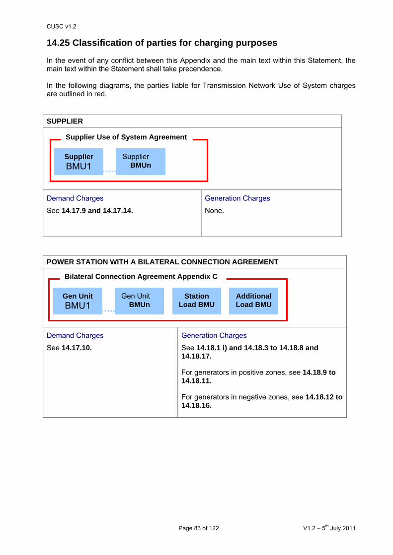
CUSC v1.2

of 122 V1.2 – 5th July 2011

14.25 Classification of parties for charging purposes In the event of any conflict between this Appendix and the main text within this Statement, the main text within the Statement shall take precendence. In the following diagrams, the parties liable for Transmission Network Use of System charges are outlined in red. SUPPLIER

Demand Charges

See 14.17.9 and 14.17.14. Generation Charges

None.

POWER STATION WITH A BILATERAL CONNECTION AGREEMENT

Demand Charges

See 14.17.10. Generation Charges

See 14.18.1 i) and 14.18.3 to 14.18.8 and 14.18.17.

For generators in positive zones, see 14.18.9 to 14.18.11.

For generators in negative zones, see 14.18.12 to 14.18.16.

Gen Unit BMU1

Gen Unit BMUn

Station Load BMU

Bilateral Connection Agreement Appendix C

Additional Load BMU

Supplier BMU1

Supplier BMUn

Supplier Use of System Agreement

CUSC v1.2

of 122 V1.2 – 5th July 2011

PARTY WITH A BILATERAL EMBEDDED GENERATION AGREEMENT

Demand Charges

See 14.17.10, 14.17.11 and 14.17.14. Generation Charges

See 14.18.1 ii).

For generators in positive zones, see 14.18.3 to 14.18.11 and 14.18.17.

For generators in negative zones, see 14.18.3 to 14.18.8 and 14.18.12 to 14.18.17.

Gen Unit BMU1

Gen Unit BMUn

Station Load BMU

Bilateral Embedded Generation Agreement Appendix C

Additional Load BMU

CUSC v1.2

of 122 V1.2 – 5th July 2011

14.26 Transmission Network Use of System Charging Flowcharts The following flowcharts illustrate the parties liable for Demand and Generation TNUoS charges and the calculation of those charges. In the event of any conflict between this Appendix and the main text within this Statement, the main text within the Statement shall take precedence. Demand Charges

NB. If the average HH metered volume of the Exempt Export BMU over the Triad

results in an import, the BMU will pay the amount of the average import x relevant

£/kW tariffIf the average HH metered volume of the

Exempt Export BMU over the Triad results in an export, the BMU will be paid

the amount of the average export x relevant £/kW tariff

BMU = BM Unit DDI = Derogated Distribution Interconnector HH = half hourly NHH = Non-half hourly

Demand ChargingStart

Average of each BMU's HH metered volume during the

Triad (x £/kW tariff)

Select appropriate

party

Average net metered import of Power Station

(including metered additional load) during the

Triad (x £/kW tariff)

Power Stations with a Bilateral Connection

Agreement or Licensable Generation with a Bilateral

Embedded Generation Agreement

Lead Party of Supplier BMU

Exemptable Generation and DDI with a Bilateral Embedded Generation

Agreement

Average metered volume of Exempt

Export BMU during the Triad (x £/kW tariff)

Each BMU's NHH metered energy consumption during 16.00-19.00 inclusive every day over the Financial Year

(x p/kWh tariff)

AND

CUSC v1.2

of 122 V1.2 – 5th July 2011

Generation Charges

Chargeable Capacity x *relevant generation tariff

Chargeable Capacity = highest TEC for Power

Station for the Financial Year

Generation Charging Start

Is the GeneratorLicensable Generation?

Liable for Generation TNUoS charges.

Chargeable Capacity x relevant generation tariff

Chargeable Capacity = ave of metered volumes during three settlement periods of highest volume between Nov to Feb

inclusive, capped by TEC applicable for the Financial Year

Ave = average BMU = BM Unit STTEC = Short-Term Transmission Entry Capacity TEC = Transmission Entry Capacity LDTEC = Limited Duration Transmission Entry Capacity

Does Generator have aBilateral Connection

Agreement withNGC?

Treating each tariffcomponent separately. Does

the Generator have a positive or negative tariff?

Positive

Negative

Yes

No

No

Yes

Not liable for Generation TNUoS charges.

STTEC/LDTEC

Short-term Chargeable Capacity x relevant short term generation tariff

Chargeable Capacity = STTEC for Power Station for STTEC period

STTEC or LDTEC of zero for negative tariff

components

* The relevant generation tariff will be net of any designated sum for generators directly connected to 132kV in Scotland. ** A full description of the short-term chargeable capacity for

LDTEC is provided in Paragraphs 5.9 and 5.14 of this document.

Short-term chargeable capacity x relevant LDTEC tariff

Short-term chargeable capacity** is the capacity purchased on a firm

profile or indicative basis and assessed on a weekly basis during

the LDTEC period.

STTEC

LDTEC

CUSC v1.2

of 122 V1.2 – 5th July 2011

14.27 Example: Determination of The Company’s Forecast for Demand Charge Purposes The Company will use the latest available settlement data for calculation of HH demand and NHH energy consumption forecasts for the Financial Year. The Financial Year runs from 1st April to 31st March inclusive and for the purpose of these examples the year April 2005 to March 2006 is used. Where the preceding year’s settlement data is not available at the time that The Company needs to calculate its forecast, The Company will use settlement data from the corresponding period in Financial Year minus two unless indicated otherwise. All values used with the examples are purely for illustrative purposes only. i) Half-Hourly (HH) Metered Demand Forecast – Existing User At the time of calculation of a HH demand forecast before the relevant Financial Year (approximately 10th March), The Company will be aware at a system level which dates will be used for the determination of Triad. However, The Company may not have settlement data at a User level if the Triad dates were to span a period that includes the latter half of February. When undertaking forecasting before the relevant Financial Year, The Company will use the User’s Triad demand for the previous year for its forecast providing it holds User settlement data for this period, thus: F = T where: F = Forecast of User’s HH demand at Triad for the Financial Year T = User’s HH demand at Triad in Financial Year minus one Where The Company determines its forecast within a Financial Year: F = T * D/P where: F = Forecast of User’s HH demand at Triad for the Financial Year T = User’s HH demand at Triad in the preceding Financial Year D = User’s average half hourly metered demand in settlement period 35 in the Financial Year

to date P = User’s average half hourly metered demand in settlement period 35 for the period

corresponding to D in the preceding Financial Year Where The Company determines its forecast before the relevant Financial Year and User settlement data for the Triad period is not available, The Company shall apply the formula immediately above (within year forecast) but substitute the following definitions for the values T, D, and P:

CUSC v1.2

of 122 V1.2 – 5th July 2011

T = User’s HH demand at Triad in the Financial Year minus two D = User’s average half hourly metered demand in settlement period 35 in the Financial Year

minus one, to date P = User’s average half hourly metered demand in settlement period 35 for the period

corresponding to D in the Financial Year minus two Example (where User settlement data is not yet available for the Triad period): The Company calculates a HH demand forecast on the above methodology at 10th March 2005 for the period 1st April 2005 to 31st March 2006. F = 10,000 * 13,200 / 12,000 F = 11,000 kWh where: T = 10,000 kWh (period November 2003 to February 2004) D = 13,200 kWh (period 1st April 2004 to 15th February 2005#) P = 12,000 kWh (period 1st April 2003 to 15th February 2004) # Latest date for which settlement data is available. ii) Non Half-Hourly (NHH) Metered Energy Consumption Forecast – Existing User F = E * D/P where: F = Forecast of User’s NHH metered energy consumption for the Financial Year E = User’s summed NHH energy consumption over the hours 16:00 to 19:00 for each day in

the preceding Financial Year D = User’s summed NHH energy consumption for the hours 16:00 to 19:00 for each day for

the Financial Year to date P = User’s summed NHH energy consumption for the hours 16:00 to 19:00 for each day for

the period corresponding to D in the preceding Financial Year Example: The Company calculates a NHH energy consumption forecast on the above methodology at 10th June 2005 for the period 1st April 2005 to 31st March 2006. F = 50,000,000 * 4,400,000 / 4,000,000 F = 55,000,000 kWh where: E = 50,000,000 kWh (period 1st April 2004 to 31st March 2005)

CUSC v1.2

of 122 V1.2 – 5th July 2011

D = 4,400,000 kWh (period 1st April 2005 to 15th May 2005#) P = 4,000,000 kWh (period 1st April 2004 to 15th May 2004) # Latest date for which settlement data is available Where forecasting before the relevant Financial Year concerned, The Company would in the above example use values for E and P from Financial Year 2003/04 and D from Financial Year 2004/05. iii) Half-Hourly (HH) Metered Demand Forecast – New User F = M * T/W where: F = Forecast of User’s HH metered demand at Triad for the Financial Year M = User’s HH average weekday period 35 demand for the last complete month for which

settlement data is available T = Total system HH demand at Triad in the preceding Financial Year W = Total system HH average weekday settlement period 35 metered demand for the

corresponding period to M for the preceding year Example: The Company calculates a HH demand forecast on the above methodology at 10th September 2005 for a new User registered from 10th June 2005 for the period 10th June 2004 to 31st March 2006. F = 1,000 * 17,000,000 / 18,888,888 F = 900 kWh where: M = 1,000 kWh (period 1st July 2005 to 31st July 2005) T = 17,000,000 kWh (period November 2004 to February 2005) W = 18,888,888 kWh (period 1st July 2004 to 31st July 2004) iv) Non Half Hourly (NHH) Metered Energy Consumption Forecast – New User F = J + (M * R/W)

CUSC v1.2

of 122 V1.2 – 5th July 2011

where: F = Forecast of User’s NHH metered energy consumption for the Financial Year J = Residual part month summed NHH metered energy consumption for the hours 16:00 to

19:00 for each day where new User registration takes place other than on the first of a month

M = User’s summed NHH metered energy consumption for the hours 16:00 to 19:00 for each

day for the last complete month for which settlement data is available R = Total system summed NHH metered energy consumption for the hours 16:00 to 19:00

for each day for the period from the start of that defined under M but for the preceding year and until the end of that preceding Financial Year

W = Total system summed NHH metered energy consumption for the hours 16:00 to 19:00

for each day for the period identified in M but for the preceding Financial Year Example: The Company calculates a NHH energy consumption forecast on the above methodology at 10th September 2005 for a new User registered from 10th June 2005 for the period 10th June 2005 to 31st March 2006. F = 500 + (1,000 * 20,000,000,000 / 2,000,000,000) F = 10,500 kWh where: J = 500 kWh (period 10th June 2005 to 30th June 2005) M = 1,000 kWh (period 1st July 2005 to 31st July 2005) R = 20,000,000,000 kWh (period 1st July 2004 to 31st March 2005) W = 2,000,000,000 kWh (period 1st July 2004 to 31st July 2004)

CUSC v1.2

of 122 V1.2 – 5th July 2011

14.28 Stability & Predictability of TNUoS tariffs Stability of tariffs The Transmission Network Use of System Charging Methodology has a number of elements to enhance the stability of the tariffs, which is an important aspect of facilitating competition in the generation and supply of electricity. This appendix seeks to highlight those elements. Each node of the transmission network is assigned to a zone. The result of this is to dampen fluctuations that would otherwise be observed at a given node caused by changes in generation, demand, and network parameters. The criteria used to establish generation zones are part of the methodology and are described in Paragraph 14.15.26. These zones are themselves fixed for the duration of the price control period. The methodology does, however, allow these to be revisited in exceptional circumstances to ensure that the charges remain reasonably cost reflective or to accommodate changes to the network. In rare circumstances where such a re-zoning exercise is required, this will be undertaken in such a way that minimises the adverse impact on Users. This is described in Paragraph 14.15.29. In addition to fixing zones, other key parameters within the methodology are also fixed for the duration of the price control period or annual changes restricted in some way. Specifically:

• the expansion constant, which reflects the annuitised value of capital investment required to transport 1MW over 1km by a 400kV over-head line, changes annually according to RPI. The other elements used to derive the expansion constant are only reviewed at the beginning of a price control period to ensure that it remains cost-reflective. This review will consider those components outlined in Paragraph 14.15.31 to Paragraph 14.15.41.

• the expansion factors, which are set on the same basis of the expansion constant and used to reflect the relative investment costs in each TO region of circuits at different transmission voltages and types, are fixed for the duration price control. These factors are reviewed at the beginning of a price control period and will take account of the same factors considered in the review of the expansion constant.

• the locational security factor, which reflects the transmission security provided under the NETS Security and Quality of Supply Standard, is fixed for the duration of the price control period and reviewed at the beginning of a price control period.

Predictability of tariffs The Company revises TNUoS tariffs each year to ensure that these remain cost-reflective and take into account changes to allowable income under the price control and RPI. There are a number of provisions within The Company’s Transmission Licence and the CUSC designed to promote the predictability of annually varying charges. Specifically, The Company is required to give the Authority 150 days notice of its intention to change use of system charges together with a reasonable assessment of the proposals on those charges; and to give Users 2 months written notice of any revised charges. The Company typically provides an additional months notice of revised charges through the publication of “indicative” tariffs. Shorter notice periods are permitted by the framework but only following consent from the Authority. These features require formal proposals to change the Transmission Use of System Charging Methodology to be initiated in October to provide sufficient time for a formal consultation and the Authority’s veto period before charges are indicated to Users.

CUSC v1.2

of 122 V1.2 – 5th July 2011

More fundamentally, The Company also provides Users with the tool used by The Company to calculate tariffs. This allows Users to make their own predictions on how future changes in the generation and supply sectors will influence tariffs. Along with the price control information, the data from the Seven Year Statement, and Users own prediction of market activity, Users are able to make a reasonable estimate of future tariffs and perform sensitivity analysis. To supplement this, The Company also prepares an annual information paper that provides an indication of the future path of the locational element of tariffs over the next five years.4 This analysis is based on data included within the Seven Year Statement. This report typically includes:

• an explanation of the events that have caused tariffs to change;

• sensitivity analysis to indicate how generation and demand tariffs would change as a result of changes in generation and demand at certain points on the network that are not included within the SYS;

• an assessment of the compliance with the zoning criteria throughout the five year period to indicate how generation zones might need to change in the future, with a view to minimising such changes and giving as much notice of the need, or potential need, to change generation zones; and

• a complete dataset for the DCLF Transport Model developed for each future year, to allow Users to undertake their own sensitivity analysis for specific scenarios that they may wish to model.

In addition, The Company will, when revising generation charging zones prior to a new price control period, undertake a zoning consultation that uses data from the latest information paper. The purpose of this consultation will be to ensure tariff zones are robust to contracted changes in generation and supply, which could be expected to reduce the need for re-zoning exercises within a price control period.

4 http://www.nationalgrid.com/uk/Electricity/Charges/gbchargingapprovalconditions/5/

CUSC v1.2

of 122 V1.2 – 5th July 2011

Section 2 – The Statement of the Balancing Services Use of

System Charging Methodology 14.29 Principles

14.29.1 The Transmission Licence allows The Company to derive revenue in respect of the Balancing Services Activity through the Balancing Services Use of System (BSUoS) charges. This statement explains the methodology used in order to calculate the BSUoS charges.

14.29.2 The Balancing Services Activity is defined in the Transmission Licence as the

activity undertaken by The Company as part of the Transmission Business including the operation of the transmission system and the procuring and using of Balancing Services for the purpose of balancing the transmission system.

14.29.3 The Company in its role as System Operator keeps the electricity system in

balance (energy balancing) and maintains the quality and security of supply (system balancing). The Company is incentivised on the procurement and utilisation of services to maintain the energy and system balance and other costs associated with operating the system. Users pay for the cost of these services and any incentivised payment/receipts through the BSUoS charge.

14.29.4 All CUSC Parties are liable for Balancing Services Use of System charges

based on their energy taken from or supplied to the National Grid system in each half-hour Settlement Period.

14.29.5 BSUoS charges comprise the following costs:

(i) The Total Costs of the Balancing Mechanism (ii) Total Balancing Services Contract costs (iii) Payments/Receipts from National Grid incentive schemes (iv) Internal costs of operating the System (v) Costs associated with contracting for and developing Balancing

Services (vi) Adjustments (vii) Costs invoiced to The Company associated with Manifest Errors and

Special Provisions. (viii) BETTA implementation costs

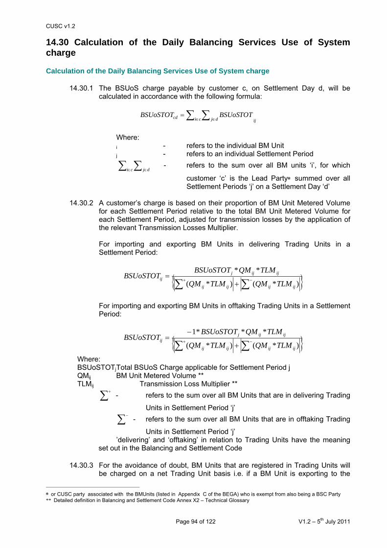
CUSC v1.2

of 122 V1.2 – 5th July 2011

14.30 Calculation of the Daily Balancing Services Use of System charge Calculation of the Daily Balancing Services Use of System charge

14.30.1 The BSUoS charge payable by customer c, on Settlement Day d, will be calculated in accordance with the following formula:

ijci djcd TOTBSUoSBSUoSTOT ∑ ∑∈ ∈=

Where: i - refers to the individual BM Unit j - refers to an individual Settlement Period

∑ ∑∈ ∈ci dj - refers to the sum over all BM units ‘i’, for which

customer ‘c’ is the Lead Party∗ summed over all Settlement Periods ‘j’ on a Settlement Day ‘d’

14.30.2 A customer’s charge is based on their proportion of BM Unit Metered Volume

for each Settlement Period relative to the total BM Unit Metered Volume for each Settlement Period, adjusted for transmission losses by the application of the relevant Transmission Losses Multiplier.

For importing and exporting BM Units in delivering Trading Units in a Settlement Period:

}{ ∑∑ −++

=)*()*(

**

ijijijij

ijijjij

TLMQMTLMQM

TLMQMBSUoSTOTBSUoSTOT

For importing and exporting BM Units in offtaking Trading Units in a Settlement Period:

}{ ∑∑ −++

−=

)*()*(

***1

ijijijij

ijijjij

TLMQMTLMQM

TLMQMBSUoSTOTBSUoSTOT

Where: BSUoSTOTj Total BSUoS Charge applicable for Settlement Period j QMij BM Unit Metered Volume ** TLMij Transmission Loss Multiplier **

∑+- refers to the sum over all BM Units that are in delivering Trading

Units in Settlement Period ‘j’ ∑−

- refers to the sum over all BM Units that are in offtaking Trading

Units in Settlement Period ‘j’ ’delivering’ and ‘offtaking’ in relation to Trading Units have the meaning set out in the Balancing and Settlement Code

14.30.3 For the avoidance of doubt, BM Units that are registered in Trading Units will

be charged on a net Trading Unit basis i.e. if a BM Unit is exporting to the

∗ or CUSC party associated with the BMUnits (listed in Appendix C of the BEGA) who is exempt from also being a BSC Party ** Detailed definition in Balancing and Settlement Code Annex X2 – Technical Glossary

CUSC v1.2

of 122 V1.2 – 5th July 2011

system and is within a Trading Unit that is offtaking from the system then the BM Unit in essence would be paid the BSUoS charge. Conversely, if a BM Unit is importing from the system in a delivering Trading Unit then the BM Unit in essence would pay the BSUoS charge. Note this includes the Interconnector BM Units that belong to the Interconnector Error Administrator.

Interconnector BM Units

14.30.4 The Lead Party of an Interconnector BM Unit will be liable for BSUoS charges based on their proportion of the total BM Unit Metered Volume of each Settlement Period adjusted for Transmission Losses by the application of the relevant Transmission Losses Multiplier.

Total BSUoS Charge (Internal + External) for each Settlement Period (BSUoSTOTjd)

14.30.5 The Total BSUoS charges for each Settlement Period (BSUoSTOTjd) for a particular day are calculated by summing the external BSUoS charge (BSUoSEXTjd) and internal BSUoS charge (BSUoSINTjd) for each Settlement Period.

jdjdjd BSUoSINTBSUoSEXTBSUoSTOT +=

External BSUoS Charge for each Settlement Period (BSUoSEXTjd)

14.30.6 The External BSUoS Charges for each Settlement Period (BSUoSEXTjd) are calculated by taking each Settlement Period System Operator BM Cash Flow (CSOBMj) and Balancing Service Variable Contract Cost (BSCCVj) and allocating the daily elements on a MWh basis across each Settlement Period in a day.

[

{ } { } ])*()*(/)*()*(*

)(

ijdijdijdijddjijdijdijdijd

ddddjdjdjd

TLMQMTLMQMTLMQMTLMQM

OMETBSCCAIncpayEXTBSCCVCSOBMBSUoSEXT

∑∑∑∑∑ −+

∈

−+++

−++++=

Calculation of the daily External Incentive Payment (IncpayEXTd)

14.30.7 In respect of each Settlement Day d, IncpayEXTd is calculated as the difference between the new total incentive payment (FKIncpayEXTd) and the incentive payment that has been made to date for the previous days from the commencement of the scheme (ξk=1≡d-1IncpayEXTk):

∑−

=

−=1

0

d

kkdd IncpayEXTTFKIncpayEXIncpayEXT

14.30.8 The forecast incentive payment made to date (from the commencement of the

scheme) (FKIncpayEXTd) is calculated as the ratio of total forecast external incentive payment across the duration of the scheme: the number of days in the scheme, multiplied by the sum of the profiling factors to date.

∑=

=d

kk

dd PFT

NDSTFYIncpayEXTFKIncpayEX

1

*

CUSC v1.2

of 122 V1.2 – 5th July 2011

Inclusion of Profiling Factors

14.30.9 Profiling factors have been included to give an effective mechanism for calculating a representative level of the incentive payments to/from The Company according to the time of year. All PFTd are assumed to be one for the duration of the current external incentive scheme.

14.30.10 The forecast External incentive payment for the duration of the External incentive scheme (FYIncpayEXTd) is calculated as the difference between the External Scheme target (Mt) and the forecast Balancing cost (FBC) subject to sharing factors (SFt) and a cap/collar (CBt).

tdttd CBFBCMSFTFYIncpayEX +−= )(*

14.30.11 The relevant value of the External incentive payment (BSUoSEXT) can then be

calculated by reference to Table 9.1 and the selection and application of the appropriate selection factors and offset dependent upon the value of the forecast Balancing Services cost (FBC).

CUSC v1.2

of 122 V1.2 – 5th July 2011

Table 9.1

Forecast Balancing Cost (FBC) Mt SFt CBt

£450,000,000 < £0 0 £15,000,000

£450,000,000 <=FBC < £550,000,000 £550,000000 0.15 £0

£550,000,000 <=FBC < £605,000,000 FBC 0 £0

£605,000,000 <= FBC < £705,000,000 £605,000,000 0.15 £0

>= £705,000,000 £0 0 -£15,000,000

14.30.12 In respect of each Settlement Day d, the forecast incentivised Balancing Cost (FBCd) will be calculated as follows:

NDSPFT

IBCFBC d

kk

d

kk

d *

1

1

∑

∑

=

==

Where:

NDS: Number of days in Scheme.

14.30.13 Daily Incentivised Balancing Cost (IBCd) is calculated as follows:

dddjdjdjddj jdd RTOMBSCCATLICNIABSCCVCSOBMIBC −−++++=∑∈)(

-15

15

Forecast Balancing

Cost (FBC)

External Incentive Payment to/from NGET

450 0

0.15

0.15

550 605

705

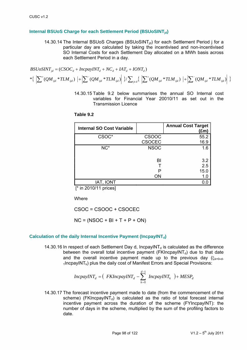
CUSC v1.2

of 122 V1.2 – 5th July 2011

Internal BSUoS Charge for each Settlement Period (BSUoSINTjd)

14.30.14 The Internal BSUoS Charges (BSUoSINTjd) for each Settlement Period j for a particular day are calculated by taking the incentivised and non-incentivised SO Internal Costs for each Settlement Day allocated on a MWh basis across each Settlement Period in a day.

{ } { })*()*(/)*()*(*

)(

ijdijdijdijddjijdijdijdijd

dddddjd

TLMQMTLMQMTLMQMTLMQM

IONTIATNCIncpayINTCSOCBSUoSINT

∑∑∑∑∑ −+

∈

−+++

++++=

14.30.15 Table 9.2 below summarises the annual SO Internal cost

variables for Financial Year 20010/11 as set out in the Transmission Licence

Table 9.2

Internal SO Cost Variable Annual Cost Target (£m)

CSOOC 55.2CSOC* CSOCEC 16.9

NSOC 1.6

BI 3.2T 2.5P 15.0

NC*

ON 1.0IAT, IONT 0.0

[* in 2010/11 prices] Where CSOC = CSOOC + CSOCEC NC = (NSOC + BI + T + P + ON)

Calculation of the daily Internal Incentive Payment (IncpayINTd)

14.30.16 In respect of each Settlement Day d, IncpayINTd is calculated as the difference between the overall total incentive payment (FKIncpayINTd) due to that date and the overall incentive payment made up to the previous day (ξk=0≡d-

1IncpayINTk) plus the daily cost of Manifest Errors and Special Provisions:

( ) dk

d

kdd MESPIncpayINTTFKIncpayINIncpayINT +−= ∑

−

=

1

0

14.30.17 The forecast incentive payment made to date (from the commencement of the

scheme) (FKIncpayINTd) is calculated as the ratio of total forecast internal incentive payment across the duration of the scheme (FYIncpayINT): the number of days in the scheme, multiplied by the sum of the profiling factors to date.

CUSC v1.2

of 122 V1.2 – 5th July 2011

k

d

k

dd PFT

NDSTFYIncpayIN

TFKIncpayIN ∑=

=1

*

14.30.18 The Company daily Internal incentive payments (IncPayINTd) are calculated by

comparing the Daily Incentivised internal operating costs (FSOINTd) against the Daily Internal Scheme Target (PTint) to set the Sharing Factor (SFint). Table 9.3 shows the respective values of these variables (in 2010/11 forecast prices).

int*)int( SFFSOINTPTTFYIncPayIN dd −=

CUSC v1.2

of 122 V1.2 – 5th July 2011

Table 9.3

FSOINTd (£) PTint (£) SFint

FSOINTd < 55,262,715 55,262,715 0.15

FSOINTd => 55,262,715 55,262,715 0.15

14.30.19 In respect of each Settlement Day d, the forecast incentivised internal controllable System Operator operating cost (FSOINTd) will be calculated as follows:

NDSPFT

CSOOCFSOINT d

kk

d

kk

d *

1

1

∑

∑

=

==

Where:

NDS: Number of days in Scheme.

14.30.20 The SO incentivised internal capital expenditure associated with balancing services activities (CSOCEC) is subject to fixed sharing factors at 15% upside and downside, to be applied each year to capital expenditure incurred which could then be added to the internal regulatory asset value (RAV).

Inclusion of Profiling Factors

14.30.21 Profiling factors have been included to give an effective mechanism for calculating a representative level of the incentive payments to/from The Company according to the time of year. All PFTk are assumed to be one for the duration of the current external incentive scheme

Manifest Errors and Special Provisions for IT system failures

14.30.22 The Company may, in certain circumstances, be required to pay compensation to BSC Parties as a result either of Manifest Errors or Special Provisions (collectively referred to as Contingency Provisions). For the avoidance of doubt charges for calling a manifest error are excluded.

14.30.23 An incentivised cost-recovery mechanism for such costs has been included

within the internal System Operator BSUoS charge element. This cost-recovery mechanism operates on a monthly basis and provides that The Company is exposed to 40% of any Contingency Provision costs invoiced to it in any month, subject to an overall monthly cap on its exposure of £250,000*.

14.30.24 Thus, if the Contingency Provision costs incurred exceed £625,000*

(£250,000*/0.4) in any month, The Company will be allowed to recover 60% of the costs it incurs up to £625,000*, and all the costs in excess of £625,000*. If costs are less than £625,000* then The Company will recover 60% of these costs.

14.30.25 The Company will calculate any allowable revenue associated with

Contingency Provisions based on the invoices received in any particular

* Subject to the indexation provisions given in the Transmission Licence

CUSC v1.2

of 122 V1.2 – 5th July 2011

month. The monthly revenue will then be recovered equally over the days in the following month. An invoice for the final month of the incentive scheme will be recovered in via the following incentive scheme in the next Financial Year.

14.30.26 The monthly cost associated with Manifest Errors and Special Provisions (CPm)

are subject to a monthly incentivised cost recovery mechanism based on a monthly Contingency Provision sharing factor (CSFm) and an offset for Contingency Provisions (OSm). The daily cost (MESPd) is calculated as follows:

NDMOSCPCSF

MESP mmmd

))(1( −−=

NDM = Number of Settlement Days in the calendar month over which these costs are recovered. The values for the 2010/11 scheme, in 2007/08 forecast prices as given in the Transmission Licence, are shown in the table below. Table 9.4

CPm CSFm OSm

0 <= CPm < £625,000 0.4 £0

CPm > £625,000 0 £250,000

CUSC v1.2

of 122 V1.2 – 5th July 2011

14.31 Settlement of BSUoS Settlement and Reconciliation of BSUoS charges

14.31.1 There are two stages of the reconciliation of BSUoS charges described below:

• Initial Settlement (SF) • Final Reconciliation (RF)

Initial Settlement of BSUoS

14.31.2 The Company will calculate initial settlement (SF) BSUoS charges in accordance with the methodology set out in Chapter 9 using the latest available data, including data from the Initial Settlement Run and the Initial Volume Allocation Run.

Reconciliation of BSUoS Charges

14.31.3 Final Reconciliation will result in the calculation of a reconciled charge for each settlement day in the scheme year. The Company will calculate Final Reconciliation (RF) BSUoS charges (with the inclusion of interest as defined in the CUSC) in accordance with the methodology set out in Chapter 9 using the latest available data, including data from the Final Reconciliation Settlement Run and the Final Reconciliation Volume Allocation Run.

Unavailability of Data

14.31.4 If any of the elements required to calculate the BSUoS charges in respect of any Settlement Day have not been notified to The Company in time for it to do the calculations then The Company will use data for the corresponding Settlement Day in the previous week. If no such values for the previous week are available to The Company then The Company will substitute such variables as it shall, at its reasonable discretion, think fit and calculate Balancing Services Use of System charges on the basis of these values. When the actual data becomes available a reconciliation run will be undertaken.

Disputes

14.31.5 If The Company or any customer identifies any error which would affect the total Balancing Services Use of System charge on a Settlement Day then The Company will recalculate the charges following resolution of the error. Revised invoices and/or credit notes will be issued for the change in charges, plus interest as set out in the CUSC. The charge recalculation and issuing of revised invoices and/or credit notes will not take place for any day where the total change in the Balancing Services charge is less than £2000.

CUSC v1.2

of 122 V1.2 – 5th July 2011

Relationship between the Statement of the Use of System Charging Methodology and the Transmission Licence

14.31.6 BSUoS charges are made on a daily basis and as such of this Statement sets out the details of the calculation of such charges on a daily basis. Customers may, when verifying charges for Balancing Services Use of System refer to the Transmission Licence which sets out the maximum allowed revenue that The Company may recover in respect of the Balancing Services Activity.

14.31.7 The Company has, where possible and appropriate, attempted to ensure that

acronyms allocated to variables within the Balancing Services charging software, and associated reporting, match with the acronyms given to those variables used within this statement.

CUSC v1.2

of 122 V1.2 – 5th July 2011

14.31.8 Balancing Services Use of System Acronym Definitions

For the avoidance of doubt “as defined in the BSC” relates to the Balancing and Settlement Code as published from time to time.

EXPRESSION ACRONYM Unit Definition

BETTA Preparation Costs BI £ As defined in the Transmission Licence

Balancing Mechanism Unit

BM Unit or BMU As defined in the BSC

Balancing service contract costs – non-Settlement Period specific

BSCCAd £ Non Settlement Period specific Balancing Contract Costs for settlement day d

Balancing Service Contract Cost BSCCj £

Balancing Service Contract Cost from purchasing Ancillary services applicable to a Settlement Period j

Balancing service contract costs – Settlement Period specific

BSCCVjd £ Settlement Period j specific Balancing Contract Costs for settlement day d

External Balancing Services Use of System charge

BSUoSEXTjd £ External System Operator (SO) Balancing Services Use of System charge applicable to Settlement Period j for settlement day d

Internal Balancing Services Use of System charge

BSUoSINTjd £ Internal System Operator (SO) Balancing Services Use of System charge applicable to Settlement Period j for settlement day d

Total Balancing Services Use of System charge

BSUoSTOTcd £

The sum determined for each customer, c, in accordance with this Statement and payable by that customer in respect of each Settlement Day d, in accordance with the terms of the Supplemental Agreement

Total Balancing Services Use of System charge

BSUoSTOTj £ Total Balancing Services Use of System Charge applicable for Settlement Period j

System Operator BM Cash Flow CSOBMj £

As defined in the Balancing and Settlement Code in force immediately prior to 1 April 2001

Forecast incentivised internal controllable System Operator cost

CSOC £ As defined in the Transmission Licence

Forecast incentivised internal System Operator capital expenditure

CSOCEC £ As defined in the Transmission Licence

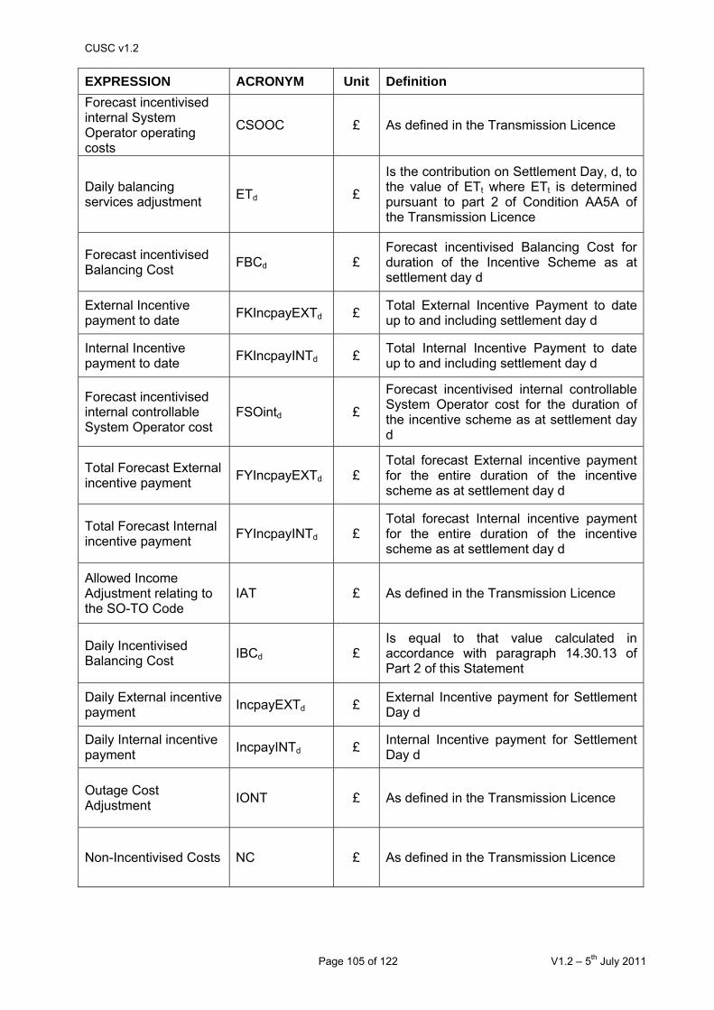
CUSC v1.2

of 122 V1.2 – 5th July 2011

EXPRESSION ACRONYM Unit Definition Forecast incentivised internal System Operator operating costs

CSOOC £ As defined in the Transmission Licence

Daily balancing services adjustment ETd £

Is the contribution on Settlement Day, d, to the value of ETt where ETt is determined pursuant to part 2 of Condition AA5A of the Transmission Licence

Forecast incentivised Balancing Cost FBCd £

Forecast incentivised Balancing Cost for duration of the Incentive Scheme as at settlement day d

External Incentive payment to date FKIncpayEXTd £ Total External Incentive Payment to date

up to and including settlement day d

Internal Incentive payment to date FKIncpayINTd £ Total Internal Incentive Payment to date

up to and including settlement day d

Forecast incentivised internal controllable System Operator cost

FSOintd £

Forecast incentivised internal controllable System Operator cost for the duration of the incentive scheme as at settlement day d

Total Forecast External incentive payment FYIncpayEXTd £

Total forecast External incentive payment for the entire duration of the incentive scheme as at settlement day d

Total Forecast Internal incentive payment FYIncpayINTd £

Total forecast Internal incentive payment for the entire duration of the incentive scheme as at settlement day d

Allowed Income Adjustment relating to the SO-TO Code

IAT £ As defined in the Transmission Licence

Daily Incentivised Balancing Cost IBCd £

Is equal to that value calculated in accordance with paragraph 14.30.13 of Part 2 of this Statement

Daily External incentive payment IncpayEXTd £ External Incentive payment for Settlement

Day d

Daily Internal incentive payment IncpayINTd £ Internal Incentive payment for Settlement

Day d

Outage Cost Adjustment IONT £ As defined in the Transmission Licence

Non-Incentivised Costs NC £ As defined in the Transmission Licence

CUSC v1.2

of 122 V1.2 – 5th July 2011


Net Imbalance Volume Cost NIj £

Total Net Energy Imbalance Volume (TQEIj)*Net Imbalance Reference Price (NIRPj)

Net Imbalance Adjustment NIAj £ As defined on the Transmission Licence

Net Imbalance Reference Price NIRPj As defined in the Transmission Licence

Non-controllable System Operator cost NSOC £ As defined in the Transmission Licence

Cost associated with the Provision of Balancing Services to others

OMd £

Is the contribution on Settlement Day, d, to the value of OMt where OMt is determined pursuant to part 2 of Condition AA5A of the Transmission Licence

Outage change allowance amount ON £ As defined in the Transmission Licence

Pension Cost Allowance P £ As defined in the Transmission Licence

Incentivised Balancing Cost daily profiling factor

PFTd The daily profiling factor used in the determination of forecast Incentivised Balancing Cost for settlement day d

Daily Internal Scheme Target PTint £ Target for the Internal Incentive scheme as

agreed with Ofgem

BM Unit Metered Volume QMij MWh As defined in the BSC

Balancing services deemed costs RTd £

Is the contribution on Settlement Day, d, to the value of RTt where RTt is determined pursuant to part 2 of Condition AA5A of the Transmission Licence

Internal Scheme sharing factor SFint Sharing Factor for the internal incentive

scheme as agreed with Ofgem

Tax Allowance T £ As defined in the Transmission Licence

Net Cost of Transmission Losses TLICj £ As defined in the Transmission Licence

Transmission Loss Multiplier TLMij As defined in the BSC

Transmission Losses Reference Price TLRPj As defined in the Transmission Licence

CUSC v1.2

of 122 V1.2 – 5th July 2011


Transmission Losses Target Volume TLTj MWh As defined in the Transmission Licence

Transmission Losses Volume TLVj MWh ∑iQMij – Sum of BM Unit Metered Volume

(QMij) over all BM units

Total System Energy Imbalance Volume TQEIj MWh

As defined in the Balancing and Settlement Code in force immediately prior to 1 April 2001

Final Reconciliation Settlement Run As defined in the BSC

Final Reconciliation Volume Allocation Run As defined in the BSC

Initial Settlement Run As defined in the BSC

Initial Volume Allocation Run As defined in the BSC

Lead Party As defined in the BSC

CUSC v1.2

of 122 V1.2 – 5th July 2011

14.32 Examples of Balancing Services Use of System (BSUoS) Daily Charge Calculations This example illustrates the operation of the Balancing Services Use of System Daily charge formula. The parameters used are for illustrative purposes only and have been chosen for ease of calculation. They do not relate to the agreed scheme for any particular year. The actual scheme parameters are shown in the main text. The example is divided into the calculation of the External System Operator cost and Internal System Operator cost elements. All daily profiling factors (PFTd) have been assumed to be one for this example. Day 1 Calculation of the Daily External SO Incentive Scheme Payment The first step is to calculate the Daily Incentivised Balancing Cost (IBC1 for day one) for that day using the following formula. These are the daily incentivised cost elements used to calculate the external SO incentive payment.

k =

kk - k k k k k =

RTOMNITLBSCCV BSCCA CSOBM = IBC 1111

1550£

0£0£50£300£200£300£800£

1111

−−+++

−−++++

Assuming that CSOBM1 = £800k

BSCCA1 = £300k BSCCV1 = £200k TL1 = £300k NI1 = -£50k

OM1 = £0k RT1 = £0k

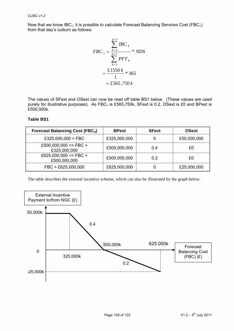
CUSC v1.2

of 122 V1.2 – 5th July 2011

Now that we know IBC1, it is possible to calculate Forecast Balancing Services Cost (FBC1) from that day’s outturn as follows:

k

k

NDSPFT

IBCFBC d

kk

d

kk

750,565£

365*1

1550£

*1

1

1

11

=

=

=

∑

∑=

=

=

=

The values of SFext and OSext can now be read off table BS1 below. (These values are used purely for illustrative purposes). As FBC1 is £565,750k, SFext is 0.2, OSext is £0 and BPext is £500,000k. Table BS1

Forecast Balancing Cost (FBCd) BPext SFext OSext

£325,000,000 < FBC £325,000,000 0 £50,000,000 £500,000,000 <= FBC >

£325,000,000 £500,000,000 0.4 £0

£625,000,000 <= FBC > £500,000,000 £500,000,000 0.2 £0

FBC > £625,000,000 £625,000,000 0 £25,000,000 The table describes the external incentive scheme, which can also be illustrated by the graph below.

-25,000k

50,000k

500,000k 625,000k Forecast

Balancing Cost (FBC) (£)

External Incentive Payment to/from NGC (£)

325,000k 0

0.4

0.2

CUSC v1.2

of 122 V1.2 – 5th July 2011

Using the values set out in the table above, the external SO incentive payment for the duration of the scheme (FYIncpayEXT) can be calculated as follows:

kkk

OSextFBCBPextSFextTFYIncpayEX

150,13£0£)750,565£000,500(£*2.0

)(* 11

−=+−=+−=

In this case the incentive payment is negative (-£13,150k) i.e. a payment from The Company. The external SO incentive payment for the entire duration of the incentive scheme (FYincpayEXT) is then used to calculate the total incentive payment to date (FKIncpayEXT), shown as follows:

027,36£

1*365

150,13£

*1

1

11

−=

−=

= ∑=

=

K

PFTNDS

TFYIncpayEXTFKIncpayEXd

kk

Where: NDS = Number of days in the external incentive scheme The final step is to calculate today’s external incentive payment (IncpayEXT1 for day one), shown as follows:

027,36£0£027,36£

01

011

−=−−=

−= ∑=−

=k

d

kIncpayEXTTFKIncpayEXIncpayEXT

Calculation of the Daily Internal SO Incentive Scheme Payment To carry this out, The Company will forecast monthly incentivised SO operating costs (CSOOC) and profile them to a daily basis. For this illustration, monthly costs for the first month of the scheme (April in our example) are assumed to be £4,500k, profiled down to a daily forecast of £150k (£450,000k divided by 30). The calculation of the forecast SO internal operating cost for day one (FSOINT1) is shown as follows:

k

k

NDSPFT

CSOOCFSOINT d

kk

d

kk

750,54£

365*1

150£

*1

1

1

11

=

=

=

∑

∑=

=

=

=

The relevant value of the internal incentive payment (FYIncpayINT1) can then be calculated by reference to Table BS2 (figures shown for illustration only) and the selection and application of

CUSC v1.2

of 122 V1.2 – 5th July 2011

the appropriate sharing factors and offset dependent upon the value of the forecast incentivised internal SO operating cost (FSOINT). Table BS2

FSOINT Ptint SFint

FSOINT < £50,000k £50,000k 0.5

FSOINT = £50,000k £50,000k 0

FSOINT > £50,000k £50,000k 0.5

The table describes the internal incentive scheme which can also be illustrated by the graph below.

Using the forecast internal operating cost for day one (FSOINT1), the internal incentive payment for the duration of the scheme (FYIncpayINT1) is calculated as follows:

kkk

SFFSOINTPTTFYIncPayIN

375,2£5.0*)750,54£000,50(£

int*)int( 11

−=−=

−=

50,000k

Internal Incentive Payment to/from NGC (£)

FSOINT (£)

0.5

0.5

0

CUSC v1.2

of 122 V1.2 – 5th July 2011

The forecast internal SO incentive payment for the duration of the scheme (FYIncpayINT1) can then be used to calculate the forecast incentive payment to date (FKIncpayINT1), shown as follows:

507,6£

1*365

375,2£

*1

1

11

−=

−=

= ∑=

=

k

PFTNDS

TFYIncpayINTFKIncpayINd

kk

The final step is to calculate the Internal incentive payment (IncpayINT1 for day one):

507,6£0£)0£507,6(£

)(01

0111

−=+−=

+−= ∑=−

=

d

kk MESPIncpayINTTFKIncpayINIncpayINT

The costs associated with Manifest Errors and Special Provisions for day 1 (MESP1) are assumed to be zero.

Calculating the External Balancing Services Use of System (BSUoS) charge for a Settlement Period j The External Balancing Services Use of System (BSUoS) charge for Settlement Period 1 on this Settlement Day 1 can now be calculated using the following formula:

[

{ } { } ])*()*(/)*()*(*

)(

1111111111111

1111111111

ijijijijjiiii TLMQMTLMQMTLMQMTLMQM


∑∑∑∑∑ −+

∈

−+++

−++++=

For simplicity, the BM Unit Metered Volume (QMij) is assumed to be the same in all half hour Settlement Periods in a Settlement Day. Therefore the daily BSUoS charge will be evenly allocated to each Settlement Period (1/48) i.e. the multiplier at the end of the equation. The illustration below shows the external BSUoS charge (BSUoSEXT11) for Settlement Period one of Settlement Day 1.

The costs of the external SO Settlement Period variables are as follows (these are the daily values included in the IBC1 equation divided by 48 Settlement Periods). CSOBM = £16,667 BSCCV = £4,167

CUSC v1.2

of 122 V1.2 – 5th July 2011

The costs of the external SO Settlement Day variables are as follows: IncpayEXT = £-36,027 BSCCA = £300k ET = £0k OM = £0k

[ ]

333,26£

499,5£167,4£667,16£

48/)0£0£300£027,36£(167,4£667,16£11

=

++=

−++−++= kkkBSUoSEXT

Calculating the Internal Balancing Services Use of System (BSUoS) charge for a Settlement Period j The Internal Balancing Services Use of System (BSUoS) charge for a Settlement Period 1 of Settlement Day 1 can now be calculated using the following formula:

{ } { })*()*(/)*()*(*

)(

11111111111111111

11111111111

iiiijiiii TLMQMTLMQMTLMQMTLMQM

IONTONBIIATPTNSOCIncpayINTCSOCBSUoSINT

∑∑∑∑∑ −+

∈

−+++

++++++++=

As with the external BSUoS charge, for simplicity, the BM Unit Metered Volume (QMij) is assumed to be the same in all half hour Settlement Periods in a Settlement Day. Therefore the daily BSUoS charge will be evenly allocated to each Settlement Period (1/48).

CUSC v1.2

of 122 V1.2 – 5th July 2011

Table BS3 below shows the annual Internal SO costs assumed for this example: Table BS3

Internal SO Cost Variable Annual Cost (£m)

CSOOC 50

CSOCEC 9

T 4

NSOC 30

P 1

BI 4

ON 3

IAT, IONT 0

Income adjustments are assumed to be zero in this example for simplicity. If it is assumed that the incentivised internal SO operating costs (CSOOC) are £150k for day 1 and the incentivised SO capital expenditure costs (CSOCEC) (assumed on target) as well as the non-incentivised elements are recovered uniformly across the year (i.e. 1/365) then:

• CSOOC (incentivised Internal SO operating costs) = £150k • CSOCEC (incentivised Internal SO capital expenditure) =£24, 657 • T (Tax allowance) = £13,699 • NSOC (Non controllable SO costs) = £82,192 • P (Pension allowance) = £2,740 • BI (BETTA preparation costs) = £32,876 • ON (Outage change allowance) = £8,219

6414£

48/)0£8219£0£0£32876£0£

740,2£192,82£699,13£657,24£)6507£(150(£11

=

++++++

++++−+= kBSUoSINT

Calculating the Total Balancing Services Use of System (BSUoS) charge for a Settlement Period 1 The final step is to calculate the Total Balancing Services Use of System (BSUoSTOT11) for a Settlement Period 1 on Settlement Day 1.

747,32£5900£333,26£

111111

=+=

+= BSUoSINTBSUoSEXTBSUoSTOT

CUSC v1.2

of 122 V1.2 – 5th July 2011

Day 2 Calculation of the Daily External SO Incentive Scheme Payment Again, the first step is to calculate the Daily Incentivised Balancing Cost for day 2 (IBC2) using the following formula:

k =

- k k k k k =

RTOM NITLBSCCV BSCCA CSOBM = IBC

950£

0£0£100£200£100£150£600£

22222222

−−+++

−−++++



OM2 = £0k RT2 = £0k With IBCd known for day one, it is possible to calculate Forecast Balancing Services Cost (FBC2) from the outturn to date as follows:

k

kk

NDSPFT

IBCFBC d

kk

d

kk

250,456£

365*2

)950£1550(£

*2

1

2

12

=

+=

=

∑

∑=

=

=

=

The values of SFext, BPext and OSext can now be read off table BS1 given previously. As FBC2 is £456,250k, SFext is now 0.4, BPext is £500,000k and OSext is 0, calculated as follows:

kkk


500,17£0£)250,456£000,500(£*4.0

)(* 22

=+−=

+−=

The external SO incentive payment for the entire duration of the incentive scheme (FYincpayEXT2) is then used to calculate the total incentive payment to date (FKIncpayEXT2), shown as follows:

CUSC v1.2

of 122 V1.2 – 5th July 2011

890,95£

2*365

500,17£

*2

1

22

=

=

= ∑=

=

k

PFTNDS

TFYIncpayEXTFKIncpayEX

d

kk

Where: NDS = Number of days in the external incentive scheme In this case the incentive payment is £95,890. Again, the final step is to calculate today’s external incentive payment (IncpayEXT2 for day two), shown as follows:

917,131£027,36£890,95£

11

022

=−−=

−= ∑=−

=

d

kkIncpayEXTTFKIncpayEXIncpayEXT

Calculation of the Daily Internal SO Incentive Scheme Payment The first step is to calculate the forecast SO internal cost for day two (FSOINT2). The same forecast of £150k for daily incentivised SO operating costs (CSOOC) used for day one is used for day two. The calculation of the forecast SO internal cost (FSOINT2) is shown as follows:

k

NDSPFT

CSOOCFSOINT d

kk

d

kk

750,54£

365*2

)000,150£000,150(£

*2

1

2

12

=

+=

=

∑

∑=

=

=

=

Using the forecast SO internal cost (FSOINT2), the forecast internal SO incentive payment for the duration of the scheme (FYIncpayINT2) can be calculated as follows (with reference to the values in Table BS2).

kkk

SFFSOINTPTTFYIncPayIN

375,2£5.0*)750,54£000,50(£

int*)int( 22

−=−=

−=


CUSC v1.2

of 122 V1.2 – 5th July 2011

014,13£

2*365

375,2£

*2

1

22

−=

−=

= ∑=

=

k

PFTNDS

TFYIncpayINTFKIncpayIN

d

kk

The final step is to calculate the Internal incentive payment (IncpayINT2 for day two).

507,6£0£)507,6£014,13£(

)(11

0222

−=+−−−=

+−= ∑=−

=

d



As all of the internal cost variables are the same on day 1 as on day 2 the incentive payments for each of these days are identical.

Calculating the External Balancing Services Use of System (BSUoS) charge for a Settlement Period j The External Balancing Services Use of System (BSUoS) charge for Settlement Period 1 of Settlement Day 2 can now be calculated using the following formula:

[

{ } { } ])*()*(/)*()*(*

)(

2222212121212

2222121212



∑∑∑∑∑ −+

∈

−+++

−++++=

As with day one, for simplicity, the BM Unit Metered Volume (QMij) is assumed to be the same in all half hour Settlement Periods in a Settlement Day. Therefore the daily BSUoS charge will be evenly allocated to each Settlement Period (1/48). The costs of the external SO Settlement Period variables are as follows: CSOBM = £12,500 BSCCV = £2,083 The costs of the external SO Settlement Day variables are as follows: IncpayEXT = £131,917 BSCCA = £150k ET = £0k OM = £0k

[ ]

456,20£

873,5£083,2£500,12£

48/)0£0£150£917,131(£083,2£500,12£12

=

++=

−++++= kkkBSUoSEXT

CUSC v1.2

of 122 V1.2 – 5th July 2011

Calculating the Internal Balancing Services Use of System (BSUoS) charge for a Settlement Period j The Internal Balancing Services Use of System (BSUoS) charge for Settlement Period 1 on Settlement Day 2 can now be calculated using the following formula:

{ } { })*()*(/)*()*(*

)(

12121212212121212

222222212


IONTONBIIATNSOCIncpayINTCSOCBSUoSINT

∑∑∑∑∑ −+

∈

−+++

++++++=

As with the external BSUoS charge, for simplicity, the BM Unit Metered Volume (QMij) is assumed to be the same in all half hour Settlement Periods in a Settlement Day (1/48). The Settlement Day 2 costs of the internal SO cost variables assigned to Settlement period 1 (based on values from Table BS3) are as follows:

6414£

82£0£0£32876£0£740,2£192,82£699,13£657,24£)6507£(150(£12

=

+++++++++−+= kBSUoSINT

Calculating the Total Balancing Services Use of System (BSUoS) charge for a Settlement Period j The final step is to calculate the Total Balancing Services Use of System (BSUoSTOT12) for Settlement Period 1 on Settlement Day 2.

870,26£6414£456,20£

121212

=+=


CUSC v1.2

of 122 V1.2 – 5th July 2011

Day 365 If we now move to the end of the year, then once again the first step is to calculate the Daily Incentivised Balancing Cost for the final day (IBC365) using the formula below:

Calculation of the Daily External SO Incentive Scheme Payment

k =

- k k k k k =

RTOM - NITLBSCCV BSCCA CSOBM = IBC

200,1£

0£0£50£200£150£200£700£

365365365365365365365365

−−+++

−++++



OM365 = £0k RT365 = £0k With ∑364IBCd assumed to be £432,000k for the previous 364 days, it is possible to calculate Forecast Balancing Services Cost (FBC365) from the outturn to date as follows:

k

kk

NDSPFT

IBCFBC d

kk

d

kk

200,433£

365*365

200,1£000,432£

*365

1

365

1365

=

+=

=

∑

∑=

=

=

=

The values of SFext, BPext and OSext can now be read off table BS1. As FBC365 is £433,200k, SFext is now 0.4, BPext is £500,000k and OSext is 0. Therefore FYIncpayEXT365 is calculated as follows:

kkk


720,26£0£)200,433£000,500(£*4.0

)(* 365365

=+−=

+−=

The external SO incentive payment for the entire duration of the incentive scheme (FYincpayEXT) is then used to calculated the total incentive payment to date (FKIncpayEXT), shown as follows:

k

k

PFTNDS

TFYIncpayEXTFKIncpayEXd

kk

720,26£

365*365

720,26£

*365

1

365365

=

=

= ∑=

=

CUSC v1.2

of 122 V1.2 – 5th July 2011

Where: NDS = Number of days in the external incentive scheme In this case the incentive payment is positive (£26,720k) i.e. a payment to The Company. As this is the last day of the scheme this represents the overall incentive payment due to The Company i.e. with reference to the graph with Table BS1 40% of the difference between £500,000k and £433,200k. Again, the final step is to calculate today’s external incentive payment (IncpayEXT365 for day 365), shown as follows: It has been assumed that the total incentive payments for the previous 364 days (ξk=0≡364IncpayEXTk) is £26,237,400.

600,482£400,237,26£000,720,26£

3641

0365365

=−=

−= ∑=−

=

d

kkIncpayEXTTFKIncpayEXIncpayEXT

Calculation of the Daily Internal BSUoS Charge Again, the first step is to calculate the forecast SO internal cost for day 365 (FSOINT365). To carry this out, The Company will forecast monthly incentivised SO operating costs (CSOOC) and profile them to a daily basis. For this illustration, monthly costs for the final month of the scheme (March in our example) are assumed to be £4,000k, profiled down to a daily forecast of £129,032 (£4,000k divided by 31). If FSOINT364 is assumed to be £52,000k, the calculation of the forecast SO internal operating cost (FSOINT365) is shown as follows:

032,129,52£

365*365

032,129£000,52£

*365

1

365

1365

=

+=

=

∑

∑=

=

=

=

k

NDSPFT

CSOOCFSOINT d

kk

d

kk

Using the forecast SO internal operating cost (FSOINT365), the forecast internal SO incentive payment for the duration of the scheme (FYIncpayINT365) can be calculated as follows:

516,064,1£5.0*)032,129,52£000,000,50(£

int*)int( 365365

−=−=

−= SFFSOINTPTTFYIncPayIN


CUSC v1.2

of 122 V1.2 – 5th July 2011

516,064,1£

365*365

516,064,1£

*365

1

365365

−=

−=

= ∑=

=

d

kkPFT

NDSTFYIncpayIN

TFKIncpayIN

In this case the incentive payment is negative (-£1,065k) i.e. a payment from The Company. As this is the last day of the scheme this represents the overall incentive payment due from The Company i.e. with reference to the graph with Table BS2 50% of the difference between £50,000k and £52,129k. The final step is to calculate the Internal incentive payment (IncpayINT365 for day 365). It has been assumed that the total incentive payments for the previous 364 days (ξk=0≡364IncpayINTk) is £1,056,145.

371,8£0£)145,056,1£516,064,1£(

)(3641

1365365365

−=+−−−=

+−= ∑=−

=

d



Calculating the External Balancing Services Use of System (BSUoS) charge for a Settlement Period j The External Balancing Services Use of System (BSUoS) charge for Settlement Period 1 of Settlement Day 365 can now be calculated using the following formula:

[

{ } { } ])*()*(/)*()*(*

)(

3653653653653651365136513651365

365365365365136513651365



∑∑∑∑∑ −+

∈

−+++

−++++=

As with day one, for simplicity, the BM Unit Metered Volume (QMij) is assumed to be the same in all half hour Settlement Periods in a Settlement Day (1/48). The costs of the external SO Settlement Period variables are as follows: CSOBM = £14,583 BSCCV = £3,125

CUSC v1.2

of 122 V1.2 – 5th July 2011

The costs of the external SO Settlement Day variables are as follows: IncpayEXT = £482,600 BSCCA = £200k ET = £0k OM = £0k

[ ]

929,31£

221,14£125,3£583,14£

48/)0£0£200£600,482(£125,3£583,14£365

=

++=

−++++= kkkBSUoSEXT

Calculating the Internal Balancing Services Use of System (BSUoS) charge for a Settlement Period j The Internal Balancing Services Use of System (BSUoS) charge for Settlement Period 1 of Settlement Day 365 can now be calculated using the following formula:

{ } { })*()*(/)*()*(*

)(

365,1365,1365,1365,1365365,1365,1365,1365,1

365365365365365365365365365365365365,1


IONTONTSHNTSPNBIIATPSCNSOCSOBRIncpayINTCSOCBSUoSINT

∑∑∑∑∑ −+

∈

−+++

++++++++++=

As with the external BSUoS charge, for simplicity, the BM Unit Metered Volume (QMij) is assumed to be the same in all half hour Settlement Periods in a Settlement Day (1/48). The Settlement Day 365 costs of the internal SO cost variables assigned to Settlement Period 1 (based on values from Table BS3) are as follows:

938,5£

0£876,32£0£740,2£192,82£699,13£24657£)8371£(032,129(£365,1

=

++++++++−+=BSUoSINT

Calculating the Total Balancing Services Use of System (BSUoS) charge for a Settlement Period j The final step is to calculate the Total Balancing Services Use of System (BSUoSTOT1365) for Settlement Period 1 on Settlement Day 365

867,37£938,5£929,31£

365,1365,1365,1

=+=


cusc - section 14 charging methodologies contents · cusc - section 14 charging methodologies...

Documents