Icarus 215 (2011) 242–252

Contents lists available at ScienceDirect

Icarus

journal homepage: www.elsevier .com/ locate/ icarus

Curvilinear features in the southern hemisphere observed by Mars GlobalSurveyor Mars Orbiter Camera

Huiqun Wang a,⇑, Anthony D. Toigo b,1, Mark I. Richardson c

a Atomic and Molecular Physics, Harvard-Smithsonian Center for Astrophysics, 60 Garden Street, Cambridge, MA 02138, USAb Center for Radiophysics and Space Research, 326 Space Sciences Building, Cornell University, Ithaca, NY 14853, USAc Ashima Research, Pasadena, CA 91106, USA

a r t i c l e i n f o

Article history:Received 23 July 2010Revised 28 May 2011Accepted 10 June 2011Available online 2 July 2011

Keywords:Atmospheres, DynamicsAtmospheres, StructureMars, Atmosphere

0019-1035/$ - see front matter � 2011 Elsevier Inc. Adoi:10.1016/j.icarus.2011.06.029

⇑ Corresponding author.E-mail address: hwang@cfa.harvard.edu (H. Wang

1 Present address: Johns Hopkins University, ApplieMD 20723, USA.

a b s t r a c t

We have used the complete set of Mars Global Surveyor (MGS) Mars Daily Global Maps (MDGMs) tostudy martian weather in the southern hemisphere, focusing on curvilinear features, including frontalevents and streaks. ‘‘Frontal events’’ refer to visible events that are morphologically analogous to terres-trial baroclinic storms. MDGMs show that visible frontal events were mainly concentrated in the 210–300�E (60–150�W) sector and the 0–60�E sector around the southern polar cap during Ls = 140–250�and Ls = 340–60�. The non-uniform spatial and temporal distributions of activity were also shown byMGS Thermal Emission Spectrometer transient temperature variations near the surface. ‘‘Streaks’’ referto long curvilinear features in the polar hood or over the polar cap. They are an indicator of the shapeof the polar vortex. Streaks in late winter usually show wavy segments between the 180� meridianand Argyre. Model results suggest that the zonal wave number m = 3 eastward traveling waves areimportant for their formation.

� 2011 Elsevier Inc. All rights reserved.

1. Introduction

Dust storms and clouds are important components of martianweather. Their morphologies, motions and distributions illuminatethe underlying circulation. They can also affect the circulationthrough radiative–dynamic feedbacks (Basu et al., 2006; Kahreet al., 2006; Rafkin, 2009; Wilson et al., 2007, 2008). Mars GlobalSurveyor (MGS) systematically monitored martian weather withthe wide angle Mars Orbiter Camera (MOC) from April 1999 toOctober 2006. Mars Reconnaissance Orbiter (MRO) Mars Color Im-ager (MARCI) has continued the daily global imaging of Mars sinceSeptember 2006; however, data from that instrument is not usedin this study. These images have provided detailed informationon dust storms and clouds (Cantor et al., 2001, 2010; Cantor,2007; Wang and Ingersoll, 2002), including global dust storms(Cantor, 2007; Strausberg et al., 2005), frontal/flushing events(Cantor et al., 2010; Hinson and Wang, 2010; Wang et al., 2003,2005; Wang, 2007) and topographic clouds (Benson et al., 2003;Cantor et al., 2010; Wang and Ingersoll, 2002). The main purposeof this paper is to present MGS MOC observations of the southernhemisphere curvilinear clouds and dust storms, including frontalevents and streaks.

ll rights reserved.

).d Physics Laboratory, Laurel,

We generally refer to curvilinear dust or cloud features whichare not apparently related to topography as ‘‘frontal events’’, ex-cept when they occur over the polar cap and/or appear as bundlesin the polar hood, in which case, we call them ‘‘streaks’’. Clouds anddust storms that exhibit other morphologies are not considered inthis paper. The morphologies, configurations and distributions ofcurvilinear clouds and dust storms suggest the influence of conver-gence and/or shear in the circulation. Here, we use ‘‘frontal events’’and ‘‘streaks’’ simply as morphological indicators, independent ofthe mesoscale dynamical mechanism, which is beyond the scopeof this paper.

The complete set of MGS Mars Daily Global Maps (MDGMs)covering the period from Ls = 150� in Mars Year 24 to Ls = 120� inMars Year 28 (May 1999–October 2006, see Clancy et al. (2000)for the definition of Mars year) has been used for this study. EachMDGM is composed using 13 pairs of red and blue global mapswaths taken by MGS MOC around 2 PM local time each day (Wangand Ingersoll, 2002). The nominal resolution of a MGS global mapswath is 7 km/pixel (some 3.75 km/pixel), and that of a MDGM is0.1� longitude � 0.1� latitude (approximately 60 km/pixel nearthe equator). Dust storms appear yellow/red, while condensateclouds appear blue/white in MDGMs. The MGS Thermal EmissionSpectrometer (TES) version 2 temperature data downloaded fromthe website http://pds-geosciences.wustl.edu have been used toprovide supplementary information in this paper. Concurrent TEStemperature data exist for the period before August 2004.MarsWRF (Richardson et al., 2007) General Circulation Model

H. Wang et al. / Icarus 215 (2011) 242–252 243

(GCM) simulations have been performed to drive an off-lineLagrangian tracer transport model (Eluszkiewicz et al., 1995; Wanget al., 2003) to examine the effects of various wind components onthe formation of wavy streaks over the south polar cap in latewinter.

2. Frontal events

Dust or ice aerosols suspended in the atmosphere can be con-centrated by winds into curvilinear features. These curvilinear fea-tures have been referred to as ‘‘frontal events’’ in studies for thenorthern hemisphere due to their morphological similarities to ter-restrial baroclinic storms in satellite images (Cantor et al., 2010;Wang et al., 2003, 2005; Wang, 2007; Wang and Fisher, 2009).While many ‘‘frontal events’’ may develop in a manner somewhat

Fig. 1. Frontal events in the south polar Mars Daily Global Maps in polar stereographic prois due to missing data in polar night. Arrows indicate frontal events. (a) Ls = 222.2� in Marin Mars Year 25 (e) Ls = 22.3� in Mars Year 27 (f) Ls = 28.2� in Mars Year 27.

similar to terrestrial baroclinic storms (near surface convergenceand upwelling), the underlying mesoscale dynamics cannot bedetermined from the images alone. Notwithstanding small-scaledynamical uncertainties, and in keeping with the original analogy,we call all non-topographic arc shaped clouds/dust storms that arenot part of the polar hood or exclusively over the polar cap as fron-tal events. In this paper, we derive statistics for the southern hemi-sphere frontal events observed in MDGMs and compare them withthe relevant results derived from TES thermal observations.

Fig. 1 shows representative southern hemisphere frontal eventsin the vicinity of the southern polar cap in mid spring (a and b), latesummer (c and d) and early fall (e and f). Most observed frontalevents lasted for between a few hours and two sols. The configura-tions of the frontal events in Fig. 1c and d indicate the presence ofplanetary waves. There appear to be vortices at the southern tipsof some arcs in Fig. 1d, analogous to those in occluded fronts. Wang

jection for the area south of 45�S. The black area at the center of subfigures c, e and fs Year 24 (b) Ls = 227.6� in Mars Year 27 (c) Ls = 354.6� in Mars Year 24 (d) Ls = 346.4�

244 H. Wang et al. / Icarus 215 (2011) 242–252

and Ingersoll (2003) showed that cloud tracked winds in the 60–80�S latitudinal band during Ls = 340–10� were generally southeast-ward (�1 m/s to �10 m/s in the meridional direction, and 5 m/s to20 m/s in the zonal direction) and occasionally southwestward inthe 90–180�E sector. Lee waves in the vicinity of the south polarcap during the fall and winter indicate eastward (westerly) zonalwinds (Wang and Ingersoll, 2002) which are consistent (via the ther-mal wind relation) with the temperature gradients derived from TESdata (Smith, 2008). MDGMs showed daily changes in the morphol-ogies, positions and configurations of the frontal events, suggestingthat they were associated with transient eddies in the atmosphere.MDGMs showed a few north–south elongated dust plumes in thesouthern tropical latitudes. There were no clear indications thatthey were related to any previous frontal events. The southernhemisphere frontal events observed by MGS did not appear to flushdust substantially equatorward, unlike some of their northernhemisphere counterparts (Wang et al., 2003, 2005; Wang, 2007).

We have archived frontal events in the southern hemisphereusing MGS MDGMs. The archive includes the solar longitude, thepositions of both end points, the length between the end pointsand the position of a representative point for each frontal event.The representative point is usually in the middle of a curvilinearfeature, at the inflection point of a curve, or at the center of a vor-tex. Vortices (Fig. 1d) were observed in about 1% of the recordedcases. Large scale curvilinear features in the polar hood or over

0 90 18Solar long

-90

-80

-70

-60

-50

-40

-30

-20

Latit

ude

150

150

150

190

190

230

230

270

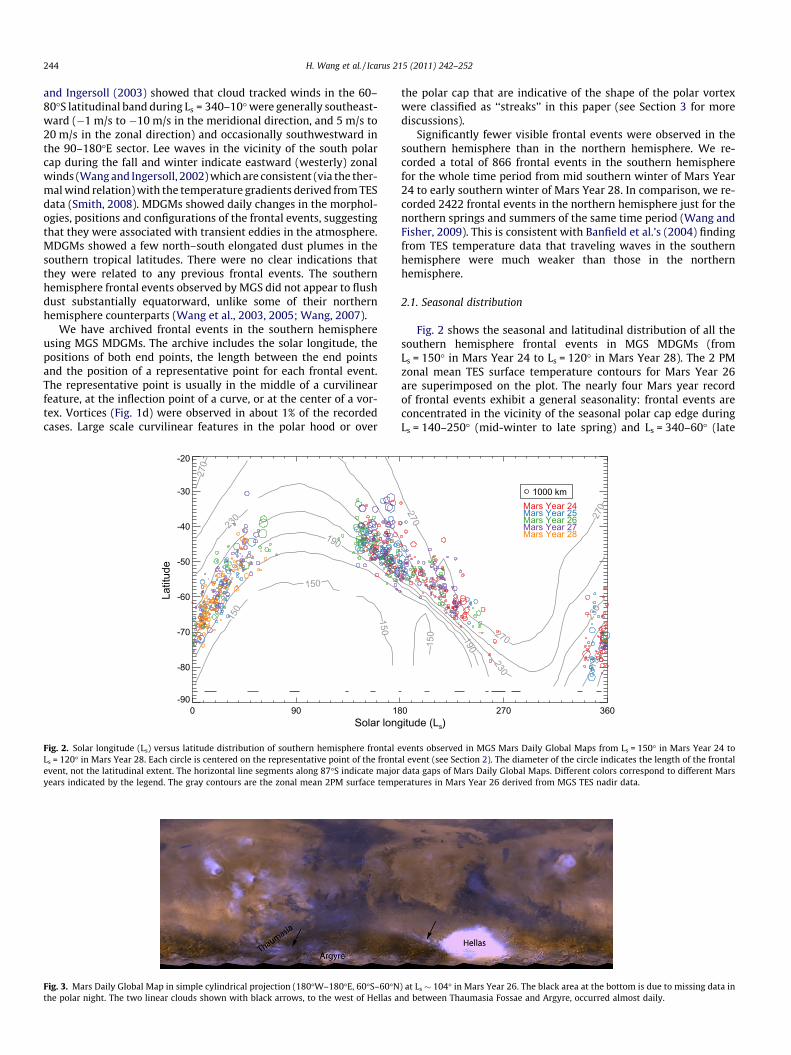
Fig. 2. Solar longitude (Ls) versus latitude distribution of southern hemisphere frontal eLs = 120� in Mars Year 28. Each circle is centered on the representative point of the frontevent, not the latitudinal extent. The horizontal line segments along 87�S indicate majoryears indicated by the legend. The gray contours are the zonal mean 2PM surface temp

Fig. 3. Mars Daily Global Map in simple cylindrical projection (180�W–180�E, 60�S–60�Nthe polar night. The two linear clouds shown with black arrows, to the west of Hellas a

the polar cap that are indicative of the shape of the polar vortexwere classified as ‘‘streaks’’ in this paper (see Section 3 for morediscussions).

Significantly fewer visible frontal events were observed in thesouthern hemisphere than in the northern hemisphere. We re-corded a total of 866 frontal events in the southern hemispherefor the whole time period from mid southern winter of Mars Year24 to early southern winter of Mars Year 28. In comparison, we re-corded 2422 frontal events in the northern hemisphere just for thenorthern springs and summers of the same time period (Wang andFisher, 2009). This is consistent with Banfield et al.’s (2004) findingfrom TES temperature data that traveling waves in the southernhemisphere were much weaker than those in the northernhemisphere.

2.1. Seasonal distribution

Fig. 2 shows the seasonal and latitudinal distribution of all thesouthern hemisphere frontal events in MGS MDGMs (fromLs = 150� in Mars Year 24 to Ls = 120� in Mars Year 28). The 2 PMzonal mean TES surface temperature contours for Mars Year 26are superimposed on the plot. The nearly four Mars year recordof frontal events exhibit a general seasonality: frontal events areconcentrated in the vicinity of the seasonal polar cap edge duringLs = 140–250� (mid-winter to late spring) and Ls = 340–60� (late

0 270 360itude (Ls)

150

190

190

230

230

270

270

270

1000 kmMars Year 24Mars Year 25Mars Year 26Mars Year 27Mars Year 28

vents observed in MGS Mars Daily Global Maps from Ls = 150� in Mars Year 24 toal event (see Section 2). The diameter of the circle indicates the length of the frontal

data gaps of Mars Daily Global Maps. Different colors correspond to different Marseratures in Mars Year 26 derived from MGS TES nadir data.

) at Ls � 104� in Mars Year 26. The black area at the bottom is due to missing data innd between Thaumasia Fossae and Argyre, occurred almost daily.

H. Wang et al. / Icarus 215 (2011) 242–252 245

summer to mid-fall). There are 462 frontal events during Ls = 140–250�, and 386 during Ls = 340–60�. Both periods have some rela-tively large frontal events whose lengths are greater than1000 km. Some frontal events near the fall equinox were substan-tially larger than the polar cap at the time, and their configurationsin MDGMs suggested the effects of planetary waves (Fig. 1c and d).In Mars Year 25, frontal events disappeared near Ls = 185� and didnot come back until about Ls = 235� (blue circles in Fig. 2), suggest-ing a possible influence of the 2001 global dust storm.

Mars Year

0 30 60 90-80

-70

-60

-50

Latit

ude

Mars Year

0 30 60 90-80

-70

-60

-50

Latit

ude

165

Mars Year

0 30 60 90L

-80

-70

-60

-50

Latit

ude

165

1.0 2.0 3.0 4.0 5.0 6.0 7.0

Fig. 4. The filled color contour shows the Ls versus latitude cross section of the standarddue to transient eddies whose wave periods are >1 sol and <30 sols. The three panels cotemperatures at 270�E and 3.7 mb.

Southern hemisphere frontal events were rarely observed in theMDGMs during Ls = 260–340�. This is consistent with TES observa-tions that traveling waves diminished in the lower atmosphere atthe southern high latitudes in summer (Banfield et al., 2003,2004). However, individual global map swaths in southern sum-mer showed occasional curvilinear dust storms near the smallsouth polar cap, especially away from the 2PM side of the image(Wang and Ingersoll, 2002; Toigo et al., 2002). Using mesoscalesimulations, Toigo et al. (2002) showed that cap edge dust lifting

24: 3.70mb

120 150 180

145

165185

205

25: 3.70mb

120 150 180

145

165

185205

26: 3.70mb

120 150 180s

145

165185

205

8.0 9.0 10.0 11.0 12.0 13.0 14.0

deviation of TES temperature (K) on the 3.7 mb constant pressure surface at 270�Errespond to Mars Year 24–26. The black contours show the corresponding mean air

246 H. Wang et al. / Icarus 215 (2011) 242–252

in mid southern summer was largely controlled by a mesoscale‘‘sea breeze’’ circulation between the polar cap and the surround-ing terrain. These dust storms did not appear clearly in MDGMsdue to their small scales and the overlap area averaging techniqueused in making the MDGMs (Wang and Ingersoll, 2002). The ab-sence of frontal events in the early summer in Fig. 2 is partly re-lated to the ‘‘selection’’ effect of MDGMs. However, larger eventsare expected to be less strongly selected against since they tendto be imaged in multiple global map swaths. Therefore, the generalpattern depicted for the larger frontal events, which are probablymore closely related to the large scale circulation, is more robust.

Southern hemisphere frontal events were also absent inMDGMs during Ls = 60–140�, as seen in Fig. 2. During the wintersolstice period, the terminator circle is very large which limitsthe visible imaging observations (Fig. 3). The southern polar hoodextended to about 50�S with apparent equatorward extension inHellas, Argyre and in the region between Thaumasia Fosse and Ar-gyre (50�W and 100�W, Fig. 3). Curvilinear clouds were observedalmost daily in the region to the west of the cloud and ice coveredHellas basin (Fig. 3). The cloud is often fibrous and analogous toterrestrial jet streak cirrus. It was not counted as a frontal eventin our catalog since it was a daily feature that appeared to be fixedto topography.

Banfield et al. (2004) showed that the transient temperaturevariation at 3.7 mb was minimal during the southern winter sol-stice period of Mars Year 25. They used a 30� Ls bin to presentthe general seasonality of transient eddies. To examine the rela-tionship between frontal events and the temperature variationsin more detail, Fig. 4 shows the seasonal and latitudinal distribu-tion of the standard deviation of temperature at 270�E and3.7 mb for transient eddies whose wave periods were between 1and 30 sols. The transient temperature perturbations were derived

0E

180E

120W

60W

90S

8.3%

10.3%

13.5%

11.5%

5.3%7.2%

0E

60E

120E

180E

120W

60W

90S 70S 50S 30S

11.7%

11.2%

8.7%

2.3%

8.1%

7.8%10.0%

12.9%

10.6%

5.7%

3.0%8.1%

(a)

(b)

Fig. 5. Longitude–latitude distribution of the southern hemisphere frontal events observeYear 28. The polar stereographically projected maps cover the area south of 30�S. The grapurpose of indicating major topography. Each circle is centered on the representative poevent (not the latitudinal extent). Different colors are for different Mars years. The percen30�S latitudinal circle. (a) All events during the year, Ls = 0–360� (b) Events from the ha

from the 2 PM TES temperatures by subtracting a linear trend ver-sus time for each 30� longitude � 2� latitude � 15� Ls bin (about 30sols). The medium number of points in the bins was about 1600.The standard deviation was calculated every 5� of Ls and was re-turned only if the number of points in the bin was at least 250.The superimposed black contours in Fig. 4 show the average tem-perature in the bin. The 270�E meridian cuts through the longitu-dinal sector where frontal events were observed most frequently(Fig. 5a). A similar pattern is obtained when the results for differentlongitudes are zonally averaged.

Fig. 4 shows that the 1–30 sol period transient eddies wereweaker during Ls = 60–140� than during Ls = 30–60� and Ls = 140–190�. The absence of frontal events in images during the wintersolstice period is consistent with the suppression of lower atmo-sphere transient eddies shown by these temperature data duringthe same period. The temperature variation during Ls = 140–190�appears stronger than that during Ls = 30–60� in Fig. 4. This ispartly due to the height of the 3.70 mb surface and the vertical dis-tribution of transient temperature variations. The Viking Landerdata showed that the surface pressure at Ls = 50� was about 20%larger than that at Ls = 150� (Hess et al., 1977). At 3.75�E and58.5�S, the topography corrected surface pressure is about 4.9 mband 4.0 mb at Ls = 50� and Ls = 150�, respectively (Smith, 2008).Consequently, the height of the 3.70 mb surface is about 2 km clo-ser to the ground during Ls = 140–190� than during Ls = 30–60�. For3.75�E and 58.5�S at Ls = 50�, the transient temperature standarddeviation at 4.75 mb is about 10% greater than that at 3.7 mb. Ban-field et al. (2004) showed that extra tropical traveling waves usu-ally had an upper level maximum at about 0.3 mb and a lower levelmaximum at the surface. The 3.70 mb surface intersects the lowerlevel maximum. It is used in Fig. 4 since it is one of the standardpressure levels for TES temperature retrievals. Despite the seasonal

60E

120E

70S 50S 30S

10.2%

10.0%

5.8%

2.1%

7.9%

8.0%

1000 km1000 km

0E

60E

120E

180E

120W

60W

90S 70S 50S 30S

8.4%

8.6%

2.3%

1.8%

7.6%

8.1%6.3%

7.1%

17.0%

18.5%

8.1%6.1%

1000 km

(c)

MY 24MY 25MY 26MY 27MY 28

d in MGS Mars Daily Global Maps from Ls = 150� in Mars Year 24 to Ls = 120� in Marsy contours are the time mean surface pressures from a MarsWRF simulation, for theint of a frontal event. The diameter of the circle indicates the length of the frontaltage of events that occurred within each 30� longitude sector is indicated along the

lf year Ls = 90–270� (c) Events from the other half year, Ls = 270–360–90�.

Fig. 6. Streaks in the south polar Mars Daily Global Maps (polar stereographic projection, 45–90�S). (a) Ls = 139.1� in Mars Year 27 (b) Ls = 179.5� in Mars Year 27 (c)Ls = 158.0� in Mars Year 24 (d) Ls = 158.5� in Mars Year 24 (e) Ls = 164.8� in Mars Year 25 (f) Ls = 165.3� in Mars Year 25.

H. Wang et al. / Icarus 215 (2011) 242–252 247

variation of the height of the constant pressure level, the pattern ofweak temperature variability during the winter solstice periodshown in Fig. 4 is robust.

2.2. Spatial distribution

Fig. 5 shows the spatial distribution of frontal events in thesouthern hemisphere observed from Ls = 150� in Mars Year 24 toLs = 120� in Mars Year 28. The percentage of events in each 30� lon-gitude sector is indicated on the plot. The observed events werepossibly located slightly downwind of the dust source regions(Wang and Fisher, 2009). Fig. 5a shows events for the full year(Ls = 0–360�). The top five most populated sectors, each accountingfor more than 10% of the population, are clustered in 60–150�Wand 0–60�E. Frontal events were observed less frequently in 60–210�E (East Hellas and its downwind region) and 0–60�W (Argyreand its downwind region). The non-uniform spatial distribution

suggests the presence of storm zones of enhanced transient eddies.Fig. 5b shows results for the winter and spring half of the year(Ls = 90–270�). The pattern is similar to that in Fig. 5a, except thatthe percentage for the 60–90�W sector (upwind of Argyre) de-creases substantially and that for the 150–180�W sector increasesto 10%. Fig. 5c shows the result for the summer and fall half of theyear (Ls = 270–90�). The top two most populated sectors accountfor 18.5% (60–90�W) and 17% (90–120�W) of the population, muchgreater than those for other sectors.

Using MGS Radio Science data between 67�S and 70�S duringLs = 134–148�, Hinson and Wilson (2002) found that there weregreater transient temperature variations in the 150–330�E (30–210�W) sector at 3 mb, and that an eastward traveling, nearly 2-sol zonal wave number m = 3 wave was dominant at the time.Their simulations using the GFDL Mars GCM reproduced these as-pects of the observations. Using TES temperature data, Banfieldet al. (2004) presented in their Fig. 19 a prominent storm zone in

-0.5 -0.4 -0.3 -0.2 -0.1

160

170

180

190

MY24 m=1

-0.5 -0.4 -0.3 -0.2 -0.1

160

170

180

190

MY24 m=2

-0.5 -0.4 -0.3 -0.2 -0.1

160

170

180

190

MY24 m=3

-0.5 -0.4 -0.3 -0.2 -0.1

160

170

180

190

MY24 m=4

-0.5 -0.4 -0.3 -0.2 -0.1

160

170

180

190

MY25 m=1

-0.5 -0.4 -0.3 -0.2 -0.1

160

170

180

190

MY25 m=2

-0.5 -0.4 -0.3 -0.2 -0.1

160

170

180

190

MY25 m=3

-0.5 -0.4 -0.3 -0.2 -0.1

160

170

180

190

MY25 m=4

-0.5 -0.4 -0.3 -0.2 -0.1

160

170

180

190

MY26 m=1

-0.5 -0.4 -0.3 -0.2 -0.1

160

170

180

190

MY26 m=2

-0.5 -0.4 -0.3 -0.2 -0.1

160

170

180

190

MY26 m=3

-0.5 -0.4 -0.3 -0.2 -0.1

160

170

180

190

MY26 m=4

0.0 0.4 0.8 1.2 1.6 2.0 2.4 2.8 3.2 3.6 4.0

Fig. 7. The amplitudes (K) of eastward traveling waves derived from the 3.7 mb MGS TES temperatures at 51�S as a function of wave frequency (r, cycle/sol, in the horizontalaxis) and Ls (in the vertical axis) for zonal wave numbers m = 1–4 and Mars Year (MY) 24–26. Wave period is the inverse of wave frequency. Negative frequency represents aneastward traveling wave.

2 For interpretation of color in Figs. 1–9, the reader is referred to the web version ofis article.

248 H. Wang et al. / Icarus 215 (2011) 242–252

the 200–300�E (60–160�W) sector and a secondary storm zone inthe 30�W–60�E sector at the southern mid and high latitudes at3.7 mb during Ls = 15–75� and Ls = 105–195� in Mars Year 24–25.Consistently, our observations using MDGMs show most frequentoccurrences of frontal events in the 210–300�E (60–150�W) sectorand the 0–60�E sector around the south polar cap (Fig. 5a).

Using the NASA Ames Mars GCM, Colaprete et al. (2005)found that due to the dynamical forcing of Hellas, Argyre andsouthern Tharsis, the south polar region of Mars was character-ized by two distinct regional climates – the cryptic sector (30�E–180�–210�E) was warm and clear and the anti-cryptic sector(150�W–0�–30�E) was cold and stormy. Fig. 5a shows that 42%of the frontal events occurred in the cryptic sector and 58% inthe anti-cryptic sector. A Chi square test for the null hypothesisthat frontal events occurred with equal frequency in the crypticand anti-cryptic sector shows that the null hypothesis should berejected at the 0.1% significance level. Therefore, there were sig-nificantly more frontal events in the cold and stormy anti-crypticsector.

3. Streaks

Kahn (1984) classified elongated features without sharp edgesacross their long axes as streaks and suggested that streaks wereprobably related to strong wind or shear. Previous observationssuggest that streaks range from local to planetary scales (Frenchet al., 1981; Kahn, 1984; Wang and Ingersoll, 2002). Therefore,the identification of streaks in images depends on the image

resolution and field of view. Viking and Mariner 9 data showedthat streaks were widespread over the planet (French et al.,1981; Kahn, 1984). In MGS MDGMs, streaks were prominent inthe polar hood (Fig. 6) and often occurred concurrently with othercloud types (Wang and Ingersoll, 2002).

In this paper, we refer to long curvilinear features as ‘‘streaks’’ ifthey are located over the polar cap and/or they form bundles in thepolar hood (Fig. 6). Both frontal events and streaks exhibit curvilin-ear structure but are in different location. Furthermore, manystreaks can be traced in multiple global map swaths that were usedto make a MDGM. Collectively, they give an impression of thewhole or part of the polar vortex (Fig. 6). We did not archivestreaks using MDGMs because of their ubiquity. The color2 schemeof the MDGMs was designed to emphasize the phenomena awayfrom the polar cap. Our frontal event catalog in Section 2 is forthe subset of transient curvilinear features that are outside the po-lar cap and polar hood. However, reprocessing a subset of MDGMs,we have noticed that in late winter (Ls = 150–180�) streaks oftendeviate from the usual roughly zonal orientation and exhibit wavystructures (Fig. 6c–f). They can either be imagined as segments ofthe polar vortex or considered as frontal events migrating overthe polar cap. Cantor et al. (2010) showed examples of northernspringtime frontal storms extending across the seasonal polarcap. We call the curvilinear features over the polar cap inFig. 6c–f ‘‘streaks’’ in this paper. They were observed most often

th

T at 51S

-2.0 -1.5 -1.0 -0.5 0.0 0.5 1.0 1.5 2.00

1

2

3

4

5

6

wav

e am

plitu

de (K

) m=1m=2m=3m=4

V at 51S

-2.0 -1.5 -1.0 -0.5 0.0 0.5 1.0 1.5 2.00

1

2

3

4

5

6

wav

e am

plitu

de (m

/s) m=1

m=2m=3m=4

T at 61S

-2.0 -1.5 -1.0 -0.5 0.0 0.5 1.0 1.5 2.0wave frequency (cycle/sol)

0

1

2

3

4

5

6

wav

e am

plitu

de (K

) m=1m=2m=3m=4

V at 61S

-2.0 -1.5 -1.0 -0.5 0.0 0.5 1.0 1.5 2.0wave frequency (cycle/sol)

0

1

2

3

4

5

6

wav

e am

plitu

de (m

/s) m=1

m=2m=3m=4

Fig. 8. Wave frequency (r, cycle/sol, horizontal axis) versus wave amplitude (vertical axis) for the 3.7 mb temperature (T, left column, K) and meridional wind (V, rightcolumn, m/s) at 51�S (top row) and 61�S (bottom row) during Ls = 150–170� derived from a (2� � 2.5� � 40) MarsWRF simulation. Negative wave frequency representseastward traveling waves, zero frequency represents stationary waves and positive frequency represents westward traveling waves. Zonal waves m = 1–4 are in black, red,blue and green, respectively.

H. Wang et al. / Icarus 215 (2011) 242–252 249

in late winter in the longitudinal sector between the 180� meridianand Argyre which is also one of the areas where frontal eventspreferentially occur (Fig. 5). Had we counted them as frontal eventsin the catalog, the general seasonal and spatial patterns of frontalevents presented in Section 2 would still have remained valid.Regardless of the classification, these long wavy features indicatethe presence of planetary waves. The positions and appearancesof the streaks varied from day to day (Fig. 6), suggesting the effectof traveling waves.

Fig. 7 shows the amplitudes of the eastward traveling waveswith zonal wave number m = 1, 2, 3 and 4 in 3.7 mb TES tempera-tures at 51�S as a function of wave frequency (r, cycles/sol, nega-tive values indicate eastward phase speed) and Ls duringLs = 150–200� of Mars Year 24–26. Westward traveling waves wereusually much weaker than eastward traveling waves (Banfieldet al., 2004). Following Wang (2007), traveling waves were derivedfrom TES temperatures using the least squares method of Wu et al.(1995) with a 16-sol sliding window for each 2� latitude � 30� lon-gitude bin. The linear temporal trend within each bin was removedbefore the wave analysis. Banfield et al. (2004) presented the an-nual cycle of traveling waves. Here, we focus on the wave spectrain late winter. Fig. 7 shows that there were different mixtures ofwave modes for different time periods and that the m = 3 waveswere dominant most of the time at this latitude. Banfield et al.(2004) pointed out that traveling waves with the same wave peri-od implied storm zones. Fig. 7 shows many such examples. In MarsYear 24, the eastward traveling 2.1 sol (r = �0.47 cycle/sol) m = 2,m = 3 and m = 4 waves were present during Ls 155–165�, the east-ward traveling 3.7 sol m = 3 and m = 2 waves were present duringLs 165–175� and the eastward traveling 2.7 sol m = 3 and m = 2waves were present during Ls 175–190�, etc. In addition to travel-ing waves, Banfield et al. (2000, 2003) derived strong amplitudes(up to 4 K or more) for zonal wave number s = 1 and s = 2 station-ary waves, and diurnal and semidiurnal tides from TES tempera-tures in the lower atmosphere of the southern extratropics in

this season. Banfield et al. (2004) pointed out that stationary waves(especially s = 1) had a much stronger effect on the zonal windsthan traveling waves.

We performed Lagrangian tracer transport experiments toexamine the effects of wind components associated with variouswave modes on the orientations of streaks and the shape of the po-lar vortex. Simulations of winds were generated with the MarsWRFMars GCM (Richardson et al., 2007), with output every 2 h, andwere used to drive an off-line Lagrangian tracer transport model.The Lagrangian tracer model uses a fourth order Runge–Kuttamethod for integration (Eluszkiewicz et al., 1995) and has previ-ously been used to study tracer transport in the Martian atmo-sphere (Wang et al., 2003). The MarsWRF GCM simulations wereconducted with prescribed dust forcing following the ‘‘MGS dustscenario’’ from the Mars Climate Database (Lewis et al., 1999). Thisspatially and temporally variable dust scenario mimics the dustdistribution in Mars Year 24 derived from TES data. The grid-pointGCM has 2� latitude � 2.5� longitude horizontal resolution anduses a 40-level vertical structure taken from the GFDL Mars GCM(Wilson and Hamilton, 1996). The model uses the same physicspackage (including radiative heating associated with CO2 and dust,diffusive mixing of heat and momentum in the boundary layer,surface and subsurface evolution of temperature, and the treat-ment of CO2 condensation and sublimation) as those describedby Lee et al. (2009) and the same surface topography, albedo, ther-mal inertia and terrain slope data as those described by Guo et al.(2009). The model has been shown to compare well with observa-tions of the zonal mean thermal structure, thermal tides, and theseasonal pressure cycle (Guo et al., 2009; Lee et al., 2009; Richard-son et al., 2007).

Fig. 8 shows the amplitude versus frequency (r) for zonal wavenumber m = 1–4 waves derived from the simulated 3.7 mb temper-ature (T) and meridional wind (V) at 51�S (top) and 61�S (bottom)during Ls = 150–170�. The analysis was performed on the 2-hourlyoutputs of the fourth year of a multiannual simulation. The wave

Fig. 9. Snapshots of Lagrangian tracer transport experiments at 26 h after simulation start. The tracers were initialized within the first 15 km of the surface in the latitudinalband between 50�S and 54�S at Ls = 165�. The winds driving the tracer transport model are from a MarsWRF simulation and are subject to the following post processing: (a)none; (b) removal of the stationary waves, diurnal and sub-1 sol components (i.e., retaining only the zonal mean and >1 sol period transients); (c) retaining only the zonalmean and stationary components; (d) including only the zonal mean, stationary, diurnal and sub-1 sol transients. The colors indicate the height of tracer above the localsurface. Tracers at low altitudes are plotted before those at high altitudes. The black contours are the simulated mean surface pressure for indicating the topography.

250 H. Wang et al. / Icarus 215 (2011) 242–252

spectra were derived using simple Fourier space–time analysis forLs = 150–170�. In agreement with the observations presented ear-lier, the simulated major wave components in temperature outputinclude the westward traveling diurnal (r = 1.0) and semidiurnal(r = 2.0) tides, stationary waves (r = 0), eastward traveling �2 sol(r � �0.5) waves and a hint of eastward traveling diurnal Kelvinwaves (r = �1.0). The near 2 sol m = 3 waves are the dominantcomponents of the eastward traveling waves, and are accompaniedby secondary m = 2 waves of the same frequencies. These wavesmade major contributions to the simulated storm zones in the low-er atmosphere (not shown). The relative importance of differentwave components depends on the latitude and also which variable(T or V) is being examined. Fig. 8 shows that the stationary waveswere dominated by s = 1 in the temperature field and by s = 3 in themeridional wind field. At 51�S, the �2 sol eastward traveling m = 3wave was comparable to the s = 1 stationary wave and the diurnaltide in the temperature field, but was substantially stronger thanthe other two in the meridional wind field. At 61�S, the �2 sol

m = 3 eastward traveling wave was about 50% weaker than thes = 1 stationary wave in the temperature field, but was comparableto the s = 3 stationary wave and stronger than the s = 1 stationarywave in the meridional wind field.

We have conducted Lagrangian tracer transport experiments toexamine the effects of various wave components in the formationof streaks observed in late winter. Fig. 9 shows the tracer distribu-tions after 26 h of Lagrangian transport. The weightless passivetracers were initialized at Ls = 165� within the first 15 km of thesurface in the latitudinal band between 50�S and 54�S (approxi-mately at the edge of the polar cap). The MarsWRF simulatedwinds were used to drive the tracer transport in Fig. 9a. The tracerdistribution exhibits apparent zonal wave number m = 3 structure.Curved bands resembling the wavy streaks in Fig. 6c–f migrateover the polar cap. The whole m = 3 pattern rotates eastwardaround the south pole at about 120�/sol as each curvilinear bandcontinued to roll up around the corresponding vortex center. Atabout 48 h, the organized features largely disappear and the

H. Wang et al. / Icarus 215 (2011) 242–252 251

tracers are mixed (not shown), suggesting that the lifetime of thesecurvilinear features is less than two sols.

Results for sensitivity studies are shown in Fig. 9b–d. In Fig. 9b,the stationary, diurnal and sub-1 sol wind components were fil-tered out, so that the winds supplied to the Lagrangian tracertransport model included only the modeled zonal mean and thetransient eddies (which were dominated by the eastward traveling�2 sol m = 3 wave). The general pattern of tracer distribution issimilar to that in Fig. 9a, except that the tracers appear to wraparound the vortex centers slightly more and the whole pattern ismore symmetric about the pole. In Fig. 9c, only the time meanwinds (including the zonal mean and stationary waves) were used.The majority of tracers are organized into an oval which is offset tothe 45�E–0�–135�W hemisphere due mostly to the effect of thes = 1 stationary wave. This is consistent with Colaprete et al.’s(2005) result from the NASA Ames Mars GCM that the south polarvortex in winter is located more toward the anti-cryptic sector. Theoval of tracers is robust after 96 h. A portion of tracers separatesfrom the oval and moves northward in Hellas and Argyre underthe influence of topographically-forced time–mean flow. Fig. 9dshows the effect of the time mean flow, diurnal and sub-1 sol tran-sients. The tracer distribution is similar to Fig. 9c, but appears tohave more irregularities along the path. The diurnal and sub-1sol transients lead to local rotations. But the amplitudes are muchsmaller than that due to the m = 3 traveling wave in Fig. 9b. Over-all, Fig. 9 suggests that the �2 sol m = 3 eastward traveling wavesare mainly responsible for producing the wavy streaks in Fig. 6c–fand for mixing the air across the south polar vortex edge in latewinter. The absence of streaks in other longitudes, which wouldbe necessary to highlight behavior of the whole polar vortex inFig. 6, is probably due to a lack of dust/condensate.

4. Summary and discussion

In this paper, we report observations and analysis of southernhemisphere curvilinear features (frontal events and streaks) de-rived from the complete set of MGS Mars Daily Global Maps forthe period from Ls = 150� of Mars Year 24 to Ls = 120� of Mars Year28. We compare the distributions of frontal events in MDGMs withtemperature variations derived from TES and other data to exam-ine the relationship between them. Our MDGM observations re-quire the presence of dust or condensate to provide visiblefeatures for analysis, and do not include cloud height information.TES temperature observations near the surface have an individualretrieval error of 2 K or more and a vertical resolution of one atmo-spheric scale height (Conrath et al., 2000). Radio Science (RS) mea-surements revealed subtle vertical temperature variations at lowaltitudes not resolvable by TES (Hinson et al., 2004), but the cover-age of RS data is sparse.

Frontal events in the southern hemisphere were observed at theedge of the south polar cap within two seasonal periods: Ls = 340–60� and Ls = 140–250�. The absence of frontal events in the earlyand mid summer is consistent with diminished transient eddyactivity in the lower atmosphere at these times derived from TESobservations (Banfield et al., 2003, 2004). During this period, thepolar area is covered by several MOC global map swaths eachday. The overlap area is averaged in a MDGM, which tends tosmooth out any dust/cloud signatures in a particular image (Wangand Ingersoll, 2002). Therefore, some small (a few hundred kilome-ters or less) frontal events near the pole may have been left out dueto the selection effect. However, larger events are not expected tobe as influenced by averaging as they appear in multiple compo-nent images. The few small dust plumes observed in MDGMs dur-ing this period were not included in our study due to the lack ofapparent curvilinear structure. There were two major episodes of

large dust import from tropical latitudes into the south polar re-gion (45–90�S) during mid-summer, and both were related to theregional dust storms initiated by flushing events in Acidalia(Ls = 316� in Mars Year 26 and Ls = 310� in Mars Year 27) (Hinsonand Wang, 2010; Wang, 2007). They were not included in thisstudy due to their amorphous morphologies.

Frontal events were rarely recorded in MDGMs during Ls = 60–140�. The lack of observable frontal events in images alone doesnot necessarily mean weaker eddies since it could possibly be re-lated to a lack of dust or condensate. However, TES temperaturesshow weaker variations in the lower atmosphere during the timeperiod. Therefore, both observations suggest suppressed transienteddies at the polar vortex edge near the surface. Banfield et al.(2004) showed that transient eddies in TES temperatures werecharacterized by a surface maximum and an upper level maxi-mum, and the seasonal behaviors of the two were different. Specif-ically, the transient variations aloft were not weaker during thistime period. The agreement between the temporal trend of frontalevents in MDGMs and that of the near surface temperature varia-tions suggest that our image observations are closely related tolower level atmospheric dynamics.

During the winter solstice period, the terminator circle is verylarge. As a result, only the outer annulus of the south polar capand hood is visible in MDGMs in this season. The south polar hoodexhibited apparent equatorward extension between ThaumasiaFossae and Argyre during this period (Fig. 3). The only apparentcurvilinear feature in this time period was located to the west ofHellas (Fig. 3). We did not include it in our catalog, since it was adaily cloud that appeared to be fixed with respect to the topogra-phy. The lack of frontal events and minimized transient eddies atthe edge of the polar vortex during the winter solstice period implythe isolation of the polar air from the rest of the atmosphere. Polarair isolation in this season is also suggested by the argon concen-trations derived from the Mars Odyssey gamma ray spectrometerdata that showed an enrichment of a factor of six of this non-con-densable gas over the south polar latitudes near the onset of south-ern winter (Sprague et al., 2004, 2007).

Frontal events were concentrated in the 210–300�E (60–150�W)sector and the 0–60�E sector around the south polar cap. These re-gions also exhibited enhanced transient temperature variations inthe lower atmosphere (Banfield et al., 2004; Hinson and Wilson,2002). Using the NASA Ames Mars GCM, Colaprete et al. (2005)found that due mainly to the dynamical forcing by Hellas andArgyre, the south polar vortex was offset to the anti-cryptic region,leading to generally stormier weather in this sector.

Curvilinear features over the polar cap or in the polar hood arecalled streaks in this paper. In MDGMs, some appear as a bundleof fibers, others as a thick line (sometimes accompanied byfibers). There are no clear distinctions in terms of morphologybetween a front and a streak. Some streaks form an oval in thepolar region, some appear as arcs, and others exhibit wavy seg-ments. A large front at the edge of the polar vortex can poten-tially transform into a streak by traveling over the polar capand merging with existing streaks. Wavy streaks were frequentlyobserved between the 180� meridian and Argyre in late winter. Awavy streak (Fig. 6c–f) may be considered as a part of the polarvortex or a frontal event that has migrated over the polar cap.Regardless of the classification, they indicate the influence ofplanetary waves. TES data and GCM simulations showed promi-nent stationary waves, diurnal tides and eastward travelingwaves during this period. Lagrangian tracer transport experi-ments suggested that m = 3 traveling waves played a key role inmaking wavy streaks in late winter.

Long term daily global monitoring is critical for studying themartian atmosphere. MGS and MRO have provided great data fordetailed studies of martian weather and climate. This paper

252 H. Wang et al. / Icarus 215 (2011) 242–252

summarizes findings from the MGS observations. Similar studiesusing MRO data will be performed in the future.

Acknowledgments

We would like to thank two anonymous reviewers for com-ments. H. Wang would like to thank the NASA Mars Data AnalysisProgram and the NASA Planetary Atmosphere program for sup-porting this effort.

References

Banfield, D., Conrath, B., Pearl, J.C., Smith, M.D., Christensen, P., 2000. Thermal tidesand stationary waves on Mars as revealed by Mars Global Surveyor ThermalEmission Spectrometer. J. Geophys. Res. 105 (E4), 9521–9537.

Banfield, D., Conrath, B.J., Smith, M.D., Christensen, P.R., Wilson, R.J., 2003. Forcedwaves in the martian atmosphere from MGS TES Nadir data. Icarus 161, 319–345.

Banfield, D., Conrath, B.J., Gierasch, P.J., Wilson, R.J., Smith, M.D., 2004. Travelingwaves in the martian atmosphere from MGS TES Nadir data. Icarus 170, 365–403.

Basu, S., Wilson, R.J., Richardson, M.I., Ingersoll, A.P., 2006. Simulation ofspontaneous and variable global dust storms with the GFDL Mars GCM. J.Geophys. Res. 111 (E9). doi:10.1029/2005JE002660 (Art. No. E09004).

Benson, J.L., Bonev, B.P., James, P.B., Shan, K.J., Cantor, B.A., Caplinger, M.A., 2003.The seasonal behavior of water ice clouds in the Tharsis and Valles Marinerisregions of Mars: Mars Orbiter Camera observations. Icarus 165, 34–52.

Cantor, B.A., 2007. MOC observations of the 2001 Mars planet-encircling dust storm.Icarus 186, 60–96.

Cantor, B.A., James, P.B., Caplinger, M., Wolff, M.J., 2001. Martian dust storms: 1999Mars Orbiter Camera observations. J. Geophys. Res. – Planets 106, 23653–23687.

Cantor, B.A., James, P.B., Calvin, W.M., 2010. MARCI and MOC observations of theatmosphere and surface cap in the north polar region of Mars. Icarus 208 (1),61–81. doi:10.1016/j.icarus.2010.01.032.

Clancy, R.T., Sandor, B.J., Wolff, M.J., Christensen, P.R., Smith, M.D., Pearl, J.C., et al.,2000. An intercomparison of ground-based millimeter, MGS TES, and Vikingatmospheric temperature measurements: Seasonal and interannual variabilityof temperatures and dust loading in the global Mars atmosphere. J. Geophys.Res. – Planets 105, 9553–9571.

Colaprete, A., Barnes, J.R., Haberle, R.M., Hollingsworth, J.L., Kieffer, H.H., Titus, T.N.,2005. Albedo of the south pole on Mars determined by topographic forcing ofatmosphere dynamics. Nature 435 (7039), 184–188. doi:10.1038/nature03561.

Conrath, B.J., Pearl, J.C., Smith, M.D., Maguire, W.C., Christensen, P.R., Dason, S., et al.,2000. Mars Global Surveyor Thermal Emission Spectrometer (TES)observations: atmospheric temperatures during aerobraking and sciencephasing. J. Geophys. Res. 105, 9509–9519.

Eluszkiewicz, J., Plumb, R.A., Nakamura, N., 1995. Dynamics of wintertimestratospheric transport in the geophysical fluid-dynamics laboratory SKYHIGeneral Circulation Model. J. Geophys. Res. 100 (D10), 20883–20900.

French, R., Gierasch, P., Popp, B., Yerdon, R., 1981. Global patterns in cloud forms onMars. Icarus 45, 468–493.

Guo, X., Lawson, W.G., Richardson, M.I., Toigo, A., 2009. Fitting the Viking Landersurface pressure cycle with a Mars General Circulation Model. J. Geophys. Res. –Planets 114. doi:10.1029/2008je003302 (Art. No. E07006).

Hess, S.L., Henry, R.M., Leovy, C.B., Ryan, J.A., Tillman, J.E., 1977. Meteorologicalresults from the surface of Mars: Viking 1 and 2. J. Geophys. Res. 82 (28), 4559–4574.

Hinson, D.P., Wang, H.Q., 2010. Further observations of regional dust storms andbaroclinic eddies in the northern hemisphere of Mars. Icarus 206, 290–305.doi:10.1016/j.icarus.2009.08.019.

Hinson, D.P., Wilson, R.J., 2002. Transient eddies in the southern hemisphere ofMars. Geophys. Res. Lett. 29. doi:10.1029/2001gl014103 (Art. No. 1154).

Hinson, D.P., Smith, M.D., Conrath, B.J., 2004. Comparison of atmospherictemperatures obtained through infrared sounding and radio occultation by

Mars Global Surveyor. J. Geophys. Res. 109 (E12002). doi:10.1029/2004JE002344.

Kahn, R., 1984. The spatial and seasonal distribution of martian clouds and somemeteorological implications. J. Geophys. Res. 89, 6671–6688.

Kahre, M.A., Murphy, J.R., Haberle, R.M., 2006. Modeling the martian dust cycle andsurface dust reservoirs with the NASA Ames General Circulation Model. J.Geophys. Res. 111 (E6). doi:10.1029/2005JE002588 (Art. No. E06008).

Lee, C., Lawson, W.G., Richardson, M.I., Heavens, N.G., Kleinbohl, A., Banfield, D.,et al., 2009. Thermal tides in the martian middle atmosphere as seen by theMars Climate Sounder. J. Geophys. Res. – Planets 114. doi:10.1029/2008je003285 (Art. No. E03005).

Lewis, S.R., Collins, M., Read, P.L., Forget, F., Hourdin, F., Fournier, R., et al., 1999. Aclimate database for Mars. J. Geophys. Res. – Planets 104, 24177–24194.

Rafkin, S.C.R., 2009. A positive radiative–dynamic feedback mechanism for themaintenance and growth of martian dust storms. J. Geophys. Res. 114.doi:10.1029/2008JE003217 (Art. No. E01009).

Richardson, M.I., Toigo, A.D., Newman, C.E., 2007. PlanetWRF: A general purpose,local to global numerical model for planetary atmospheric and climatedynamics. J. Geophys. Res. – Planets 112. doi:10.1029/2006je002825 (Art. No.E09001).

Smith, M.D., 2008. Spacecraft observations of the martian atmosphere. Annu. Rev.Earth Planet. Sci. 36, 191–219. doi:10.1146/annurev.earth.36.031207.124335.

Sprague, A.L., Boynton, W.V., Kerry, K.E., Janes, D.M., Hunten, D.M., Kim, K.J., et al.,2004. Mars’ south polar Ar enhancement: A tracer for south polar seasonalmeridional mixing. Science 306 (5700), 1364–1367. doi:10.1126/science.1098496.

Sprague, A.L., Boynton, W.V., Kerry, K.E., Janes, D.M., Kelly, N.J., Crombie, M.K., et al.,2007. Mars’ atmospheric argon: Tracer for understanding martian atmosphericcirculation and dynamics. J. Geophys. Res. 112 (E3). doi:10.1029/2005JE002597(Art. No. E03S02).

Strausberg, M.J., Wang, H.Q., Richardson, M.I., Ewald, S.P., Toigo, A.D., 2005.Observations of the initiation and evolution of the 2001 Mars global duststorm. J. Geophys. Res. – Planets 110. doi:10.1029/2004JE002361.

Toigo, A.D., Richardson, M.I., Wilson, R.J., Wang, H.Q., Ingersoll, A.P., 2002. A firstlook at dust lifting and dust storms near the south pole of Mars with amesoscale model. J. Geophys. Res. 107 (E7). doi:10.1029/2001JE001592 (Art.No. 5050).

Wang, H.Q., 2007. Dust storms originating in the northern hemisphere during thethird mapping year of Mars Global Surveyor. Icarus 189, 325–343. doi:10.1016/j.icarus.2007.01.014.

Wang, H.Q., Fisher, J.A., 2009. North polar frontal clouds and dust storms on Marsduring spring and summer. Icarus 204, 103–113. doi:10.1016/j.icarus.2009.05.028.

Wang, H.Q., Ingersoll, A.P., 2002. Martian clouds observed by Mars Global SurveyorMars Orbiter Camera. J. Geophys. Res. – Planets 107. doi:10.1029/2001JE001815.

Wang, H.Q., Ingersoll, A.P., 2003. Cloud-tracked winds for the first Mars GlobalSurveyor mapping year. J. Geophys. Res. 108 (E9). doi:10.1029/2003JE002107(Art. No. 5110).

Wang, H.Q., Richardson, M.I., Wilson, R.J., Ingersoll, A.P., Toigo, A.D., Zurek, R.W.,2003. Cyclones, tides, and the origin of a cross-equatorial dust storm on Mars.Geophys. Res. Lett. 30. doi:10.1029/2002GL016828.

Wang, H.Q., Zurek, R.W., Richardson, M.I., 2005. Relationship between frontal duststorms and transient eddy activity in the northern hemisphere of Mars asobserved by Mars Global Surveyor. J. Geophys. Res. – Planets 110. doi:10.1029/2005JE002423.

Wilson, R.J., Hamilton, K., 1996. Comprehensive model simulation of the thermaltides in the martian atmosphere. J. Atmos. Sci. 53 (9), 1290–1326.

Wilson, R.J., Neumann, G.A., Smith, M.D., 2007. Diurnal variation and radiativeinfluence of martian water ice clouds. Geophys. Res. Lett. 34 (2). doi:10.1029/2006GL027976 (Art. No. L02710).

Wilson, R.J., Lewis, S.R., Montabone, L., Smith, M.D., 2008. Influence of water iceclouds on martian tropical atmospheric temperatures. Geophys. Res. Lett. 35(7). doi:10.1029/2007GL032405 (Art. No. L07202).

Wu, D.L., Hays, P.B., Skinner, W.R., 1995. A least-squares method for spectral-analysis of space–time series. J. Atmos. Sci. 52 (20), 3501–3511.