curves and surfaces - graphics.stanford.edu

1

Curves and Surfaces

CS148, Summer 2010

Siddhartha Chaudhuri

2

(Möb

ius

strip

: Ind

uctiv

eloa

d@W

ikip

edia

)

Möbius strip: 1 surface, 1 edge Klein bottle: 1 surface, no edges

3

Curves and Surfaces

● Curve: 1D set● Generally defined as f : ℝ → X, where X is some space

● Surface: 2D set● Generally defined as f : ℝ2 → X

● X is the space in which the set is embedded● Dimension of curve/surface ≠ Dimension of X!● E.g. plane is 2D surface embedded in 3D

4

Parametric Curves● p = f(t)

● f(...) is a vector-valued function

● Line: p = tu + p0

● u is direction of line, p0 is any point on the line

● Ray: t ≥ 0● Line segment: t ∈ [0, 1]

● Circle: (x, y) = (rcos t, rsin t)

5

Parametric Curves

Parametric curve f(time) traced out by a stunt plane 6

Parametric Surfaces● p = f(s, t)● Plane: p = su + tv + p0

● u, v are any two directions in the plane● p0 is any point on it

● Sphere: (x, y, z) = (rcos s sin t, rsin s sin t, rcos t)● Note: (s, t) provide a set of texture coordinates for

the surface● A d-dimensional set is defined with d parameters

7

Implicit Forms

● Curve embedded in 2D: f(x, y) = 0● f(...) is a scalar-valued function● Line: ax + by + 1 = 0● Circle: x2 + y2 – r2 = 0

● Surface embedded in 3D: f(x, y, z) = 0● Plane: ax + by + cz + 1 = 0● Sphere: x2 + y2 + z2 – r2 = 0

● In general, an implicitly defined set consists of points p s.t. f(p) = 0

8

Implicit Forms● Also called level set or isocontour

● Usually written as f(p) = c, which can be recast to the standard form: f(p) – c = 0

Level sets of the Earth's terrain

height(x, y) = constant

(Banaue rice terraces, the Philippines)

9

Normal to Curve Embedded in 2D

● From parametric form:Normal to p = f(t) = (x(t), y(t)) is

● From implicit form:Normal to f(x, y) = 0 is

∂ f∂ x ,∂ f∂ y

Normal

Tang

ent−d y

d t, d x

d t

10

Normal to Surface Embedded in 3D

● From parametric form:Normal to p = f(s, t) is

● From implicit form:Normal to f(x, y, z) = 0 is

∂ f∂ s

× ∂ f∂ t

∂ f∂ x , ∂ f∂ y , ∂ f∂ z

Normal

Tangentplane

(Oleg Alexandrov)

11

Caution!● Normals can point in two opposing directions

● Choose a consistent convention● For closed surfaces we usually take the outward

direction

● Many formulæ require unit normals● Divide by the length of the normal to unitize

or ?

12

Piecewise Linear Approximation of Curve● Straight lines are easier to process and display

than curves!

13

Piecewise Linear Approximation of Surface

Triangle Mesh

● Polygons are easier to process and display than curved surfaces!

14

Polygon Meshes● Set of edge-connected planar polygons (usually

triangles or quads)● Faces share vertices and edges● To avoid repeating vertices, store each vertex once● Each face stored as set of indices into the vertex list

● Connectivity of faces also called mesh topology● Normal at vertex often estimated

as average of unit normals ofall faces sharing that vertex● Useful in practice, but less precise

than differentiating original surface

15

Displaying Polygon Meshes

● Flat shading: Compute shading at face center, use for entire face

● Per-vertex (Gouraud) shading: Compute shading at vertices, interpolate to face interiors

● Per-fragment (Phong) shading: Interpolate normals to face interiors, compute shading at each fragment● Don't confuse with Phong

reflection model!

Qua

lity

Spee

d

16


Flat shading Per-vertex(Gouraud)shading

Per-fragment(Phong)shading

(Camillo Trevisan)

17


Flat shading Per-vertex(Gouraud)shading

Per-fragment(Phong)shading

(Paul Heckbert) 18

Controlling a Curve

● Specify control parameters at a few locations● Points● Tangents● …

● Make the curve conform to these parameters

Control pointControl point

ControlControlpointpoint

ControlControlpointpoint

(Get

ty Im

ages

)

19

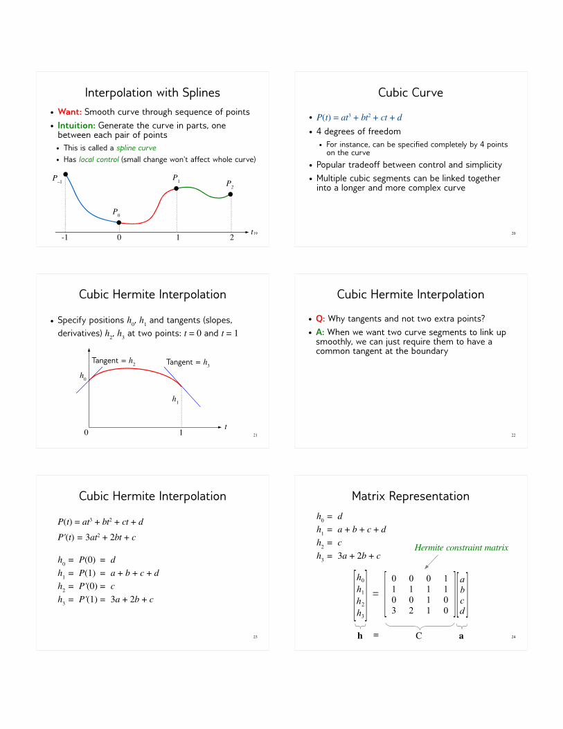
Interpolation with Splines● Want: Smooth curve through sequence of points● Intuition: Generate the curve in parts, one

between each pair of points● This is called a spline curve● Has local control (small change won't affect whole curve)

t0 1 2-1

P0

P–1 P1 P2

20

Cubic Curve

● P(t) = at3 + bt2 + ct + d● 4 degrees of freedom

● For instance, can be specified completely by 4 points on the curve

● Popular tradeoff between control and simplicity● Multiple cubic segments can be linked together

into a longer and more complex curve

21

Cubic Hermite Interpolation

● Specify positions h0, h1 and tangents (slopes, derivatives) h2, h3 at two points: t = 0 and t = 1

Tangent = h2 Tangent = h3

h0

h1

t0 1 22


● Q: Why tangents and not two extra points?● A: When we want two curve segments to link up

smoothly, we can just require them to have a common tangent at the boundary

23


P(t) = at3 + bt2 + ct + dP'(t) = 3at2 + 2bt + c

h0 = P(0) = dh1 = P(1) = a + b + c + dh2 = P'(0) = ch3 = P'(1) = 3a + 2b + c

24

Matrix Representationh0 = dh1 = a + b + c + dh2 = ch3 = 3a + 2b + c

[h0

h1

h2

h3] = [ 0 0 0 1

1 1 1 10 0 1 03 2 1 0 ][abcd ]

h C a=

Hermite constraint matrix

25

Matrix Representation

h = Ca ⇒ a = C-1h

[abcd ] = [ 2 −2 1 1−3 3 −2 −10 0 1 01 0 0 0 ][h0

h1

h2

h3]

Hermite basis matrix 26

Matrix Representation of Polynomials

P t = [a b c d ] [t3

t2

t1 ]

27


P t = [h0 h1 h2 h3 ] [ 2 −3 0 1−2 3 0 01 −2 1 01 −1 0 0 ] [t

3

t2t1 ]

(C-1)T

28


P t = [h0 h1 h2 h3 ] [H 0t H 1t H 2t H 3t

]Hermite basis functions

P(t) = Σ hi Hi(t)i = 0

3

29

Hermite Basis Functions

H0(t) = 2t3 – 3t2 + 1H1(t) = –2t3 + 3t2

H2(t) = t3 – 2t2 + tH3(t) = t3 – t2

H0(t)H1(t)

H2(t)

H3(t)

30

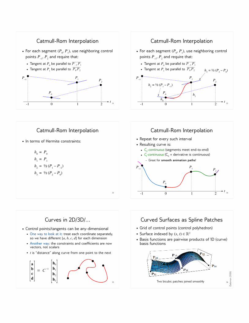
Catmull-Rom Interpolation

● Want: Smooth curve through sequence of points● Intuition: A plausible tangent at each point can be

inferred directly from the data● Now use Hermite interpolation

P0

t0 1 2-1

P1 P2

P–1

31

Catmull-Rom Interpolation● For each segment (P0, P1), use neighboring control

points P–1, P2 and require that:● Tangent at P0 be parallel to● Tangent at P1 be parallel to

P0

t0 1 2-1

P–1 P1 P2

P−1 P1

P0P2

32


h0 t0 1 2-1

h1

h3 = ½ (P2 – P0)

h2 = ½ (P1 – P–1)

P0

P–1 P1 P2

● For each segment (P0, P1), use neighboring control points P–1, P2 and require that:● Tangent at P0 be parallel to● Tangent at P1 be parallel to

P−1 P1

P0P2

33


● In terms of Hermite constraints:

h0 = P0

h1 = P1

h2 = ½ (P1 – P–1)h3 = ½ (P2 – P0)

34

Catmull-Rom Interpolation● Repeat for every such interval● Resulting curve is:

● C0-continuous (segments meet end-to-end)● C1-continuous (C0 + derivative is continuous)

– Great for smooth animation paths!

t0 1 2-1

P0

P–1 P1 P2

35

Curves in 2D/3D/…● Control points/tangents can be any-dimensional

● One way to look at it: treat each coordinate separately, so we have different [a, b, c, d] for each dimension

● Another way: the constraints and coefficients are now vectors, not scalars

● t is “distance” along curve from one point to the next

[abcd ] = C−1 [h0

h1

h2

h3]

36

Curved Surfaces as Spline Patches● Grid of control points (control polyhedron)● Surface indexed by (s, t) ∈ ℝ2

● Basis functions are pairwise products of 1D (curve) basis functions

Two bicubic patches joined smoothly

(Sal

omon

200

6)

curves and surfaces - graphics.stanford.edu

Documents