curves and jacobians : number extractors and … and jacobians : number extractors and efficient...

Curves and Jacobians : number extractors and efficientarithmeticRezaeian Farashahi, R.

DOI:10.6100/IR637900

Published: 01/01/2008

Document VersionPublisher’s PDF, also known as Version of Record (includes final page, issue and volume numbers)

Please check the document version of this publication:

• A submitted manuscript is the author's version of the article upon submission and before peer-review. There can be important differencesbetween the submitted version and the official published version of record. People interested in the research are advised to contact theauthor for the final version of the publication, or visit the DOI to the publisher's website.• The final author version and the galley proof are versions of the publication after peer review.• The final published version features the final layout of the paper including the volume, issue and page numbers.

Link to publication

General rightsCopyright and moral rights for the publications made accessible in the public portal are retained by the authors and/or other copyright ownersand it is a condition of accessing publications that users recognise and abide by the legal requirements associated with these rights.

• Users may download and print one copy of any publication from the public portal for the purpose of private study or research. • You may not further distribute the material or use it for any profit-making activity or commercial gain • You may freely distribute the URL identifying the publication in the public portal ?

Take down policyIf you believe that this document breaches copyright please contact us providing details, and we will remove access to the work immediatelyand investigate your claim.

Download date: 30. Aug. 2018

https://doi.org/10.6100/IR637900

https://research.tue.nl/en/publications/curves-and-jacobians--number-extractors-and-efficient-arithmetic(82195b29-e95a-46c5-a596-95ebffd43b7b).html

.

Curves and Jacobians:

Number Extractors

and Efficient Arithmetic

Reza Rezaeian Farashahi

Curves and Jacobians:Number Extractors

and Efficient Arithmetic

PROEFSCHRIFT

ter verkrijging van de graad van doctoraan de Technische Universiteit Eindhoven, op gezag van de

Rector Magnificus, prof.dr.ir. C.J. van Duijn, voor eencommissie aangewezen door het College voor

Promoties in het openbaar te verdedigenop maandag 27 oktober 2008 om 16.00 uur

door


geboren te Teheran, Iran

Dit proefschrift is goedgekeurd door de promotoren:

prof.dr.ir. H.C.A. van Tilborgenprof.dr. T. Lange

Copromotor:dr. G.R. Pellikaan

CIP-DATA LIBRARY TECHNISCHE UNIVERSITEIT EINDHOVEN

Rezaeian Farashahi, Reza

Curves and Jacobians: Number Extractors and Efficient Arithmetic/ door Reza Rezaeian Farashahi. -Eindhoven : Technische Universiteit Eindhoven, 2008.Proefschrift. - ISBN 978-90-386-1410-6NUR 918Subject headings: Algebraic geometry, Cryptology2000 Mathematics Subject Classification: 11G20, 14H40, 14H52, 14G50, 94A60

Promotor: prof.dr.ir. H.C.A. van Tilborg (Technische Universiteit Eindhoven)Promotor: prof.dr. T. Lange (Technische Universiteit Eindhoven)

Copromotor: dr. G.R. Pellikaan (Technische Universiteit Eindhoven)

Commissie:prof.dr.ir. A.E. Brouwer (Technische Universiteit Eindhoven)prof.dr. S.J. Edixhoven (Universiteit Leiden)prof.dr.dr.h.c. G. Frey (Universitat Duisburg-Essen)prof.dr. I.E. Shparlinski (Macquarie University)

Ministry of Science, Research and Technology

Islamic Republic of Iran

The work in this thesis is supported by the Ministry of Science, Research andTechnology of I. R. Iran under scholarship no. 800.147.

c© Reza Rezaeian Farashahi 2008. All rights are reserved. Reproduction in wholeor in part is prohibited without the written consent of the copyright owner.

Printing: Eindhoven University Press

Cover design: S.E. Baha

Contents

Preface v

1 Introduction 11.1 Extractors on curves and Jacobians . . . . . . . . . . . . . . . . . . 31.2 Efficient arithmetic on elliptic curves . . . . . . . . . . . . . . . . . 7

2 Mathematical Background 92.1 Finite fields notation . . . . . . . . . . . . . . . . . . . . . . . . . . 92.2 Arithmetic of curves . . . . . . . . . . . . . . . . . . . . . . . . . . 112.3 Elliptic curves . . . . . . . . . . . . . . . . . . . . . . . . . . . . . . 17

2.3.1 Edwards curve . . . . . . . . . . . . . . . . . . . . . . . . . 182.4 Weil descent . . . . . . . . . . . . . . . . . . . . . . . . . . . . . . . 192.5 Hyperelliptic curves . . . . . . . . . . . . . . . . . . . . . . . . . . 202.6 The Jacobian of hyperelliptic curves . . . . . . . . . . . . . . . . . 21

2.6.1 On the Jacobian of genus-2 curves . . . . . . . . . . . . . . 232.7 Kummer surface . . . . . . . . . . . . . . . . . . . . . . . . . . . . 232.8 A surface related to the Jacobian in odd characteristic . . . . . . . 242.9 A surface related to the binary Jacobian . . . . . . . . . . . . . . . 282.10 Deterministic extractor . . . . . . . . . . . . . . . . . . . . . . . . . 32

2.10.1 Extractor for a subgroup . . . . . . . . . . . . . . . . . . . 332.11 Deterministic extractors for varieties . . . . . . . . . . . . . . . . . 35

3 Norm and Trace Varieties 393.1 Norm variety . . . . . . . . . . . . . . . . . . . . . . . . . . . . . . 403.2 Trace variety . . . . . . . . . . . . . . . . . . . . . . . . . . . . . . 43

3.2.1 Example: trace surface for binary elliptic curve . . . . . . . 44

4 Extractors for Binary Elliptic Curves 474.1 The extractor for the elliptic curve E . . . . . . . . . . . . . . . . . 48

i

4.1.1 The extractor for E . . . . . . . . . . . . . . . . . . . . . . 484.1.2 Analysis of the extractor . . . . . . . . . . . . . . . . . . . . 53

4.2 The extractor for a subgroup . . . . . . . . . . . . . . . . . . . . . 55

5 The Quadratic Extension Extractor for (Hyper)elliptic Curves 575.1 The quadratic extension extractor . . . . . . . . . . . . . . . . . . 58

5.1.1 The extractor for C . . . . . . . . . . . . . . . . . . . . . . . 585.1.2 Analysis of the extractor . . . . . . . . . . . . . . . . . . . . 63

5.2 Examples . . . . . . . . . . . . . . . . . . . . . . . . . . . . . . . . 645.2.1 The extractor for a subgroup of F∗q2 . . . . . . . . . . . . . 645.2.2 The extractor for elliptic curves . . . . . . . . . . . . . . . . 65

6 Extractors for Jacobians of Genus-2 Curves in Odd Characteristic 676.1 The extractors for the Jacobian . . . . . . . . . . . . . . . . . . . . 68

6.1.1 The sum extractor for the Jacobian . . . . . . . . . . . . . 686.1.2 The product extractor for the Jacobian . . . . . . . . . . . 696.1.3 Analysis of the extractors . . . . . . . . . . . . . . . . . . . 70

6.2 Proofs of theorems . . . . . . . . . . . . . . . . . . . . . . . . . . . 716.2.1 Proof of the sum extractor theorem . . . . . . . . . . . . . 726.2.2 Proof of the product extractor theorem . . . . . . . . . . . 76

6.3 Extractors for the Kummer surface . . . . . . . . . . . . . . . . . . 786.3.1 The sum extractor for the Kummer surface . . . . . . . . . 796.3.2 The product extractor for the Kummer surface . . . . . . . 80

7 Extractors for Jacobians of Genus-2 Binary Curves 837.1 The extractors for the Jacobian . . . . . . . . . . . . . . . . . . . . 84

7.1.1 The sum extractor . . . . . . . . . . . . . . . . . . . . . . . 847.1.2 The product extractor . . . . . . . . . . . . . . . . . . . . . 857.1.3 Analysis of the extractors . . . . . . . . . . . . . . . . . . . 857.1.4 The extractor for a subgroup . . . . . . . . . . . . . . . . . 86

7.2 Proofs of theorems . . . . . . . . . . . . . . . . . . . . . . . . . . . 877.2.1 Relation between discriminant and the case distinction . . . 887.2.2 Proof of the sum extractor theorem . . . . . . . . . . . . . 897.2.3 Proof of the product extractor theorem . . . . . . . . . . . 95

8 Binary Edwards Curves 998.1 Binary Edwards curves . . . . . . . . . . . . . . . . . . . . . . . . . 1008.2 The addition law . . . . . . . . . . . . . . . . . . . . . . . . . . . . 1028.3 Complete binary Edwards curves . . . . . . . . . . . . . . . . . . . 1078.4 Explicit addition formulas . . . . . . . . . . . . . . . . . . . . . . . 1098.5 Doubling . . . . . . . . . . . . . . . . . . . . . . . . . . . . . . . . 1118.6 Differential addition . . . . . . . . . . . . . . . . . . . . . . . . . . 114

9 Concluding Remarks 121

ii

References 125

Summary 133

Curriculum Vitae 135

List of Notations 137

Index 139

iii

Preface

ذرد ه د ن ا د د جان و و د م ن ا This momentous time of my life would have been impossible without the support,enthusiasm and encouragement of many incredibly precious people. I devote thispreface to thank them.

First of all, I would like to express my deep and sincere gratitude to my supervisors,Henk van Tilborg, Tanja Lange and Ruud Pellikaan for giving me the possibilityto work under their supervision. Thanks to Henk for accepting me as a Ph.D.student in his group and for his friendship throughout these four years. Tanjaand Ruud were my daily supervisors and always ready to discuss various issuesconcerning my research and to answer my questions. This work would not havebeen possible without their support and encouragement, and I am grateful fortheir valuable friendship.

The results in this thesis are the fruits of joint work with my distinguished co-authors: Dan Bernstein, Bas Edixhoven, Tanja Lange, Ruud Pellikaan and AndreySidorenko. So my best thanks go to them. I would also like to express my greatappreciation to the rest of my co-authors: Wouter Castryck, Steven Galbraith,Berry Schoenmaker and Igor Shparlinski with whom I worked on papers that arenot in this thesis. It was my pleasure to work with all of them, and it made merealize the value of working together as a team. Thank you all.

The members of my thesis committee are gratefully acknowledged for reading thethesis, providing useful comments and being present in my defense session. It wasmy privilege to have Andries Brouwer, Bas Edixhoven, Kees van Hee, Tanja Lange,Ruud Pellikaan, Igor Shparlinski and Henk van Tilborg in the reading committeeand Gerhard Frey in the defense opposition.

In the past four years, I had the opportunity to cooperate with many people andseveral groups from different institutes. For these opportunities, I am obliged to

Gerhard Frey from Institute of Experimental Mathematics, University of Duisburg-Essen, Germany, Bas Edixhoven from Mathematical Institute, University of Lei-den, The Netherlands, Steven Galbraith from Mathematics Department, RoyalHolloway University of London, UK, and Igor Shparlinski from the Departmentof Computing, Macquarie University, Australia. Although I could not fit all theresults of cooperations with these good colleagues in this thesis, they have cer-tainly influenced the state of my mind and hence they are indirectly present inthis thesis.

The great working atmosphere in the Coding Theory and Cryptology group atEindhoven University of Technology is certainly never forgotten. I express my bestthanks to all members of the group for being so friendly, helping me from timeto time, organizing enjoyable meetings, social events and tea breaks. Discussionsessions with the supervisors Henk, Ruud, Tanja, Benne, Berry, Dan, and withstudents Ellen, Andrey, Mehmet, Jose, Peter (Birkner), Christiane, Peter (vanLiesdonk), Michael, Peter (Schwabe), Sebastiaan and Gaetan were a nice way tothink about new research problems and learn from their research interest andproblems. Anita, Bram, Wil and Henny completed this nice group as well. I havebeen fortunate to be an office-mate of many nice people in the group. I would liketo thank all my office-mates for their help, conversations and discussions. I alsowould like to thank all members of Security group as well as the Discrete Algebraand Geometry group for sharing the friendly and creative atmosphere with ourgroup.

My PhD study was supported by a scholarship from the Ministry of Science,Research and Technology of I. R. Iran. I would like to take this opportunityto thank them for their support. I also would like to thank Farhad Rahmati andMohammad Hossein Abdollahi, Mohammad Nazemi, academic representatives anddirectors of Iranian students in Europe for their help.

I would like to express my gratitude to my professors at the University of Tehranand Chamran University of Ahvaz for their advice and insights. Special thanks goto Mansoor Motamedi (my ex-supervisor). I would also like to thank my teachersin Maleksabet high school whom I am greatly indebted to them for their help andencouragement that stimulated my interest in mathematics.

I express my best thanks to the Iranian families Baha, Farshi, Fatemi, Eslami,Mousavi, Moosavi Nejad, Nikoufard, Sedghi, Shojaei and Talebi for their help andsupport and for the great time we had with them. I would also like to expressmy gratitude to Mohammad Ali Abam, Ehsan Baha, Mohammad Eslami, Mo-hammad Farshi, Hamed Fatemi, Amir Hossein Ghamarian, Kamyar Malakpoor,Mohammad Reza Mousavi, Mohammad Moosavi Nejad, Iman Mosavat, MahmoudNikoufard, Pooyan Sakian, Mohammad Samimi, Saeed Sedghi, Hamid Shojaei,Saeid Talebi and many other wonderful Iranian students in the Netherlands fortheir kind friendship. Finally, thanks to many other good friends, specially themembers of Saturday’s soccer team.

vi

I am grateful beyond expression to my dearest family. Words cannot express theextent to which I feel indebted and grateful to them for all their unconditionalhelp and support throughout my whole life and in particular, during the last fouryears. My special thanks go for my wife Maryam, my daughter Fatemeh and myson Mohammad for sharing the beautiful moments of their life with me. I dedicatethis thesis to them, with love and gratitude.


September 2008

vii

Chapter 1

Introduction

Algebraic curves over finite fields are being extensively studied in the context ofpublic-key cryptographic schemes. Koblitz [65] and Miller [82] were the first toshow that the group of rational points on an elliptic curve over a finite field canbe used for the discrete logarithm problem in a public-key cryptosystem. Ellipticcurves have received a lot of attention throughout the past 2 decades and manyresearchers became interested in computational problems related to the efficientarithmetic in the group law and solving the discrete logarithm problem in thegroup [8, 23, 50]. They have been proposed for applications in cryptographydue to their fast group law and because so far no subexponential attack on theirdiscrete logarithm problem is known (see [23]). The most efficient methods forsolving the DL problem for ordinary elliptic curve have exponential running time.For supersingular elliptic curves there exist subexponential methods, (see [80]) sosupersingular elliptic curves should be avoided for DL based cryptosystem.

Compared to traditional cryptosystems like RSA, ECC offers equivalent securitywith smaller key sizes, which results in faster computations, lower power con-sumption, as well as memory and bandwidth savings. This is especially usefulfor mobile devices which are typically limited in terms of their CPU, power andnetwork connectivity.

Koblitz, [66], was the first to suggest using the discrete logarithm problem in theJacobian of a hyperelliptic curve over a finite field in public key cryptography.Hyperelliptic curves of genus 2 are undergoing intensive study (e.g. see [23]) andhave been shown to be competitive with elliptic curves in speed and security andfor suitably chosen curves the best attacks are generic attacks. Many researchershave optimized genus 2 arithmetic so that in several families of curves they are

2 Chapter 1 Introduction

faster than elliptic curves [46, 47, 73]. The security of genus 2 hyperelliptic curvesis in general assumed to be similar to that of elliptic curves of the same groupsize [44].

The use of the Kummer surface associated to the Jacobian of a genus 2 curve isproposed for faster arithmetic (see [25, 46, 68]). The scalar multiplication on theJacobian can be used to define a scalar multiplication on the Kummer surface.This can be applied in cryptography; e.g. in the Diffie-Hellman protocol (see [93]).In addition, it is shown there, that solving the discrete logarithm problem on theJacobian is polynomial time equivalent to solving the discrete logarithm problemon the Kummer surface.

The problem of converting random points of a group into random bits has severalcryptographic applications. Examples are key derivation functions, key exchangeprotocols and the design of cryptographically secure pseudorandom number gen-erators. For instance, at the end of the Diffie-Hellman key exchange protocol (e.g.the well-known (hyper)elliptic curve Diffie-Hellman protocol), the parties agree ona common secret element of the group G. This element is indistinguishable from auniformly random group element under the decisional Diffie-Hellman assumption(denoted by DDH). However, the binary representation of the common secret el-ement is distinguishable from a uniformly random bit-string of the same length.Therefore one has to convert this group element into a bit string statistically closeto uniformly random. The classical solution is to use a hash function. Then,the indistinguishability cannot be proved in the standard model but only in therandom oracle model. An alternative solution is to use extractors for the group G.

An extractor on a set is a function that converts a random element of the set toa random bit-string, which is statistically close to a uniformly random bit-string.There exists vast literature on extractors in the general setting of a map betweenarbitrarily distributed (long) bit-strings to almost uniformly distributed (shorter)bit-strings (see [21, 40, 89, 96] and references there in).

The security of extractors is based on standard assumptions and so they allow usto avoid the random oracle model for key exchange protocols. The DLP in a groupG can always be solved in time O(

√#G) and for suitably chosen groups there are

no faster attacks known. To match security levels, the key for a symmetric cipherwith k bits key should be derived from a group element of a group of size 2k bits,i.e. the extractor could reduce the bit-length by at least a factor of 2.

In this thesis, we deal with number extractors based on elliptic and hyperellipticcurves. Then, we generalize the number extractors to the genus-2 Jacobians andassociated Kummer surfaces. As a second related topic we study fast arithmeticon binary elliptic curves and introduce a new representation for these curves.

1.1 Extractors on curves and Jacobians 3

1.1 Extractors on curves and Jacobians

The construction of provable and more efficient pseudorandom generators based onsome standard and non-standard assumptions is a requirement for cryptographicschemes. The literature on pseudorandom number generators on curves and Jaco-bians is mostly concerned with studying the distribution of the coordinates or thecoordinate pairs [5, 28, 53, 61, 71, 72, 90] or considers only the extreme case ofextracting one bit per point [48]. The extractors for curves and Jacobians, whichoutput as many bits as possible, can be used to construct cryptographically securepseudorandom generators.

So far, several deterministic randomness extractors for elliptic curves have beenproposed. Kaliski [61] shows that if a point is taken uniformly at random from theunion of an elliptic curve and its quadratic twist then the x-coordinate of this pointis uniformly distributed in the finite field. Then, the TAU technique [20] allows toextract almost all the bits of the abscissa of a point of the union of an elliptic curveand its quadratic twist. This technique uses the idea in [61], that if a point is takenuniformly at random from the union of an elliptic curve and its quadratic twistthen the abscissa of this point is uniformly distributed in the finite field. Gurel[49] proposed an extractor for an elliptic curve defined over a quadratic extensionof a prime field. It extracts almost half of the bits of the abscissa of a point on thecurve. Another extractor for elliptic curves over prime fields is proposed by Gurelin the same paper. However, the latter extracts significantly less than half of thebits of the abscissa of a point on the curve.

A simple way to construct an extractor based on curves, Jacobians and in generalvarieties over finite fields is as follows. Consider a variety of dimension n over afinite field Fq. Suppose each point of this variety is represented by n independentcoefficients plus some other dependent coefficients. An extractor can be definedthat, for a given point on the variety, outputs some k independent coefficients ofthe point, where k is a positive integer less than or equal to n. This means, theextractor outputs k numbers in Fq, from a point of the variety that is compactlyrepresented by n numbers in Fq. Obviously a smaller k implies a smaller output,but also a more uniformly distributed output. This extractor can be generalizedto a variety over an extension finite field of Fq by means of restriction techniquesfrom the extension field to the ground field Fq.

Our contributions. In Chapters 4 and 5, we present a simple and efficient extrac-tor, called Ext, based on (hyper)elliptic curves defined over a quadratic extensionof the finite field Fq. For a given point on the (hyper)elliptic curve, our extrac-tor outputs the first Fq-coefficient of the x-coordinate of the point. Further, onecan define an extractor that, for a given point on the curve, outputs an Fq-linearcombination of both coefficients of the x-coordinate of this point. The analysisof our extractor shows that, for randomly distributed points on the curve, thedistribution of the Fq-sequence is indistinguishable from the uniform distribution


on Fq.

We note that the x-coordinate of a uniformly random point on a (hyper)ellipticcurve can be easily distinguished from a uniformly random field element. Ourextractor, Ext, provides only part of the x-coordinate and thereby avoids theobvious problem; the proof shows that actual uniformity is achieved. Our approachis somewhat similar to the basic idea of pseudorandom generators proposed byGong et al. [48] and Beelen and Doumen [5] in that they use a function that mapsthe set of points on an elliptic curve to a set of smaller cardinality. In the formerreference, this function outputs the trace map of the x-coordinate of the point ona binary curve. So, each point gives rise only to one bit. The latter studied moregeneral functions so that some more bits per point can be obtained. Our aim is toextract as many bits as possible while keeping the output distribution statisticallyclose to uniform.

So far, the all known deterministic randomness extractors for elliptic curves can beapplied only for elliptic curves over odd prime fields and their extensions, althoughin many cases elliptic curves over binary fields can be implemented more efficientlyin hardware (see, e.g., [50]). Till now, the problem of constructing an efficientdeterministic extractor for elliptic curves over binary fields remained open.

In Chapter 4, the extractor Ext is presented for a binary elliptic curve E definedover Fq2 , where q = 2` and ` is a positive integer. So, by means of Ext, exactly `bits can be extracted from a given point on E. Also, in this chapter, we presentan extractor for the main subgroup G of E, where E has minimal 2-torsion. Thisextractor has more practical applications in cryptography, if both ` and the orderof G are primes. The results of this chapter are based on [33, 34].

In many cases, it is recommended to use elliptic curves over F2m , where m is aprime number. Recall that in Chapter 4 we consider elliptic curves over E(F2m),where m = 2`. To the best of our knowledge, the DL problem for the latter curvesis as hard as the one for the former curves provided that the GGHS attack isinfeasible, that is, ` is a prime number and ` 6= 127 (for more details see [22, 41,42, 52, 79, 81]). The finite fields F2178 ,F2226 ,F21018 and F21186 are suggested forelliptic curve cryptography in [22]. For these fields the GGHS attack is infeasible.Furthermore by the ghost bit bases technique, the arithmetic operations in thesefields can be performed more efficiently than in prime extension of F2 of the samesize (see [54, 92]).

An efficient pseudorandom generator based on elliptic curves is proposed by Barkerand Kelsey [4]. Unfortunately, their generator (called Dual Elliptic Curve gener-ator) is insecure, the reason being that random bits are extracted from randompoints of the elliptic curve in an improper way [16, 35, 85]. Replacing the extractorused by Barker and Kelsey with one of our extractors yields a pseudorandom gen-erator which is provably secure under the DDH assumption and the x-logarithmassumption [16].

1.1 Extractors on curves and Jacobians 5

In Chapter 5, the extractor Ext is described for (hyper)elliptic curves over finitefields with odd characteristic. In particular, the definition of Ext for elliptic curvesis similar to the proposed extractor in [49], yet the analysis is improved by meansof our proof techniques. The results of this chapter are based on [32].

The main part of the analysis of extractor Ext is the counting part; i.e., to findbounds on the number of points of all fibers of Ext. In other words, we need toestimate the number of points on the curve with a fixed first coefficient of thex-coordinate. We can find these estimates by means of the Weil descent techniqueand Hasse-Weil Theorem as follows. First we consider the Weil descent of thecurve from a quadratic extension to the ground field. So, we obtain a surface overFq, algebraically defined by a system of two equations with 4 variables. Then,we fix the corresponding variable to the first coefficient of the x-coordinate. Thismeans, we intersect the Weil descent surface with a coordinate hyperplane, so weobtain in general a curve defined by a system of two equations with 3 variables.Next, we need to estimate the number of points on this intersection. We can usethe resultant technique or Groebner basis algorithm to eliminate one variable inthe later system and obtain a bi-variate equation. A curve can be defined by thisbi-variate equation and the number of points on this curve can be shown to bealmost equal to the number of points on the corresponding fiber of Ext. Afterthat, we investigate the irreducibility of this curve. If it is absolutely irreducible,we examine the singularity and compute the genus of the curve. Further, weobtain bounds for the number of points on this curve by means of the Hasse-WeilTheorem. This implies a solution for the counting problem. We note that theestimates by the later curve are not tight, so a suitable transformation is neededto obtain tight estimates.

Our approaches to finding bounds on the number of points of the fibers of Extin Chapters 4 and 5 are similar to the above, but we use alternative restrictiontechniques. We replace the Weil descent surface with other related surfaces. Theyare called trace and norm surfaces and used respectively in Chapters 4 and 5.These surfaces are algebraically defined by one equation over Fq with 3 variables.Then, we consider the intersections of these surfaces with coordinate hyperplanes.We show that the number of points on each intersection equals the number ofpoints of the related fiber of Ext. Next, we need to estimate the number of pointson the intersections. We show that these intersections are in general absolutelyirreducible nonsingular curves. After that, by means of the Hasse-Weil Theoremfor these curves, we obtain estimates for the number of points on fibers of Ext.

We used the trace and the norm techniques instead of the Weil-descent, because ofthe following reasons. First of all, with these techniques, it is easier to handle thealgebraic analysis of the geometry of the hyperplanes intersections. So, our claimsare provided with shorter proof techniques. Secondly, by the norm and the tracetechniques, tight estimates can be obtained after the intersection step. We notethat, in the first approach, because of using the resultant technique, the equations


of the intersections are of higher degree and tight estimates can not be obtaineddirectly.

In Chapter 3, the idea of the trace surface is generalized to curves of the Artin-Schreier form. In fact, an Artin-Schreier curve defined over an extension of Fq ofdegree n is related to an n-dimensional hypersurface defined over Fq. This gener-alization is based on a particular case, namely that of binary elliptic curves overquadratic extension finite fields, introduced as the trace surface in [33]. Also, theidea of the norm surface is generalized to the Kummer curves. Indeed, a Kummercurve over an extension of Fq of degree n is related to an n-dimensional hypersur-face defined over Fq. For the particular case of hyperelliptic curves over quadraticextension fields Fq2 , the norm surface was proposed in [32]. We hope that thestudy of the geometry of the intersections of the trace and the norm hypersurfaceswith hyperplanes enables us to generalize the definition of the extractor Ext toArtin-Schreier and Kummer curves over finite fields.

In Chapters 6 and 7, we present two simple and efficient extractors for Jacobians ofgenus-2 hyperellipic curves. They are called the sum and the product extractors.The sum (respectively the product) extractor, for a given point D on the Jacobianof a hyperelliptic curve H over Fq, outputs the sum (respectively the product) of x-coordinates of points on H in the support of D, considering D as a reduced divisor.It is shown that, if the point D is chosen uniformly at random in the Jacobianof H over Fq, the element extracted from the point D is indistinguishable from auniformly random variable in Fq.

Again, the main part in the sum and product extractors is the counting part.We follow a similar above approach to finding bounds on the number of pointson the fibers of these extractors. In Chapter 2, we introduce a surface relatedto the Jacobian of genus 2-hyperelliptic curves over Fq. This surface is definedby an algebraic equation with 3 variables, where the two independent variablescorrespond to the sum and the product of the x-coordinates of points on H in thesupport of reduced divisors in the Jacobian of H over Fq. We obtain bounds on thenumber of points on the intersections of this surface with coordinate hyperplanes,which enables us to estimate the number of points on the fibers of the sum andproduct extractors.

In Chapter 6, we describe the sum and the product extractors for Jacobians ofgenus-2 hyperellipic curves over Fq with odd characteristic. Further, in this chap-ter, modified versions of the sum and the product extractors are proposed for theKummer surface associated to the Jacoobian of a genus-2 hyperelliptic curve. Theresults of this chapter are based on [29].

In Chapter 7, we extend definitions of the sum and the product extractors toJacobians of genus-2 hyperellipic curves over binary fields. Further, the modifiedsum and product extractors are suggested for the main subgroup of the Jacobian ofH over Fq with group order 2m, where m is odd. We note that, for cryptographic

1.2 Efficient arithmetic on elliptic curves 7

application m, the order of the subgroup, is chosen to be prime. The results ofthis chapter are based on [30].

1.2 Efficient arithmetic on elliptic curves

The points on a Weierstrass-form elliptic curve

y2 + a1xy + a3y = x3 + a2x2 + a4x + a6

include not only the affine points (x1, y1) satisfying the curve equation but alsoan extra point at infinity serving as the neutral element. The standard formulasto compute a sum P + Q fail if P is at infinity, or if Q is at infinity, or if P + Qis at infinity, or if P is equal to Q. Each of these possibilities needs to be testedfor and handled separately; a complete addition algorithm is produced by gluingtogether several incomplete addition formulas.

This plethora of cases has caused a seemingly neverending string of problems forimplementors of elliptic-curve cryptography, especially in cryptographic hardwaresubject to side-channel attacks. Consider, for example, computing nP +mQ. Atypical two-scalar-multiplication algorithm would double P , add P , add Q, etc.,where the exact pattern of additions and doublings depends on the values of nand m. What happens if 3P = Q? Does the implementation take the time tosee that 3P = Q and to switch from the addition formulas to doubling formulas?Can the attacker detect the switch through timing analysis, power analysis, etc.?If the implementation fails to check for 3P = Q, what does it end up comput-ing? What about 3P = −Q? Can an attacker trigger failure cases—and incorrectcomputations—by choosing inputs cleverly? Can these failures compromise cryp-tographic security?

Some papers have presented “unified” addition formulas that can be used fordoublings. See, e.g., [12], [14], [15], [58], and [74]; for overviews see [9, Section 5],[57], and [69]. “Strongly unified” addition formulas eliminate the need to checkfor equal inputs. However, they do not eliminate the need to check for inputs andoutputs at infinity and for other exceptional cases. The exceptional-points attackpresented in [56] targets the exceptional cases in these unified formulas.

Edwards curves. Edwards [26] proposed a new normal form for elliptic curvesand gave an addition law that is remarkably symmetric in the x and y coordinates.In the recent paper [9], Bernstein and Lange show for fields F with char(F) 6= 2that if d is not a square in F then the affine points on the “Edwards curve”

x2 + y2 = 1 + dx2y2

form a group. The affine addition law introduced by Edwards in [26] is completefor this curve, as are the fast projective formulas introduced in [9].


“Complete” is stronger than “unified”: it means that the addition formulas workfor all pairs of input points. There are no troublesome points at infinity. Inparticular, the neutral element of the curve is an affine point (0, 1).

If F is finite then approximately 1/4 of all elliptic curves over F are birationallyequivalent to complete Edwards curves, i.e., Edwards curves with non-square d.The formulas in [9] can therefore be used for elliptic-curve computations, and inparticular for elliptic-curve cryptography.

Implementors can—although they are not forced to!—gain speed by switching fromthe addition formulas to dedicated doubling formulas when the inputs are knownto be equal. Bernstein and Lange show, for typical scalar-multiplication problems,that their addition formulas and doubling formulas for Edwards curves use fewermultiplications than the best available formulas for previous curve shapes.

Our Contributions. In Chapter 8, we present a new shape for ordinary ellipticcurves over fields of characteristic 2. Using the new shape, we present the firstcomplete addition formulas for binary elliptic curves, i.e., addition formulas thatwork for all pairs of input points, with no exceptional cases. If n ≥ 3 then thecomplete curves cover all isomorphism classes of ordinary elliptic curves over F2n .

In this chapter, we also present dedicated doubling formulas for these curves. Thedoubling formulas are the first complete doubling formulas in the literature, withno exceptions for the neutral element, points of order 2, etc. Finally, we presentcomplete formulas for differential addition, i.e., addition of points with knowndifference. Indeed, our doubling formulas and differential-addition formulas areextremely fast. The results of this chapter are based on [11].

Chapter 2

Mathematical Background

In this chapter we define the important notions that are used throughout thisthesis. We also provide the mathematical background that is necessary for under-standing the context of the number extractors based on curves and Jacobians.

We let N0 denote the set of non-negative integers and R0 the set of non-negativereal numbers. A field is denoted by F and its algebraic closure by F. Further, letF∗ denote the set of nonzero elements of F. The finite field with q elements isdenoted by Fq, and its algebraic closure by Fq. The cardinality of a finite set S isdenoted by #S. We make a distinction between a variable x and a specific value xin F.

2.1 Finite fields notation

Consider the finite field Fqn , where q is a prime power and n is a positive integer.Then Fqn is a vector space over Fq. Let {α1, α2, . . . , αn} be a basis of Fqn over Fq.This means that every element x in Fqn can be uniquely represented by the formx = x1α1 +x2α2 + . . .+xnαn, where xi ∈ Fq. We recall [75] that {α1, α2, . . . , αn}is a basis of Fqn over Fq if and only if

∣∣∣∣∣∣∣∣∣α1 α2 . . . αnαq1 αq2 . . . αqn...

......

αqn−1

1 αqn−1

1 . . . αqn−1

n

∣∣∣∣∣∣∣∣∣ 6= 0.

10 Chapter 2 Mathematical Background

Let φ : Fq −→ Fq be the Frobenius map defined by φ(x) = xq. Let φ(i), for apositive integer i, be the i-th iterated function of φ. That is φ(i)(x) = xq

i

.

Let x ∈ Fqn . The norm and trace of x are defined by the formulas

NFqn/Fq(x) =

n−1∏i=0

φ(i)(x) and TrFqn/Fq(x) =

n−1∑i=0

φ(i)(x).

Now, we extend the definition of norm and trace to the field of fractions of amultivariate polynomial ring as follows.

Let Fq(x1,x2, . . . ,xn) be the field of fractions of the polynomial ring Fq[x1,x2, . . . ,xn].We extend the Frobenius map φ from Fq to Fq(x1,x2, . . . ,xn) linearly by meansof φ(xi) = xi, for 1 ≤ i ≤ n. Similarly, let φ(i) be the i-th iterated function of φ.Clearly, f is a rational function defined over Fq if and only if φ(f) = f .

Whenever the fields are clear from the context we omit the indices, i.e., we writeN(x) = NFqn/Fq

(x) and Tr(x) = TrFqn/Fq(x) for x ∈ Fqn .

For a rational function f in Fqn(x1,x2, . . . ,xn), we define

NFqn/Fq(f) =

n−1∏i=0

φ(i)(f) and TrFqn/Fq(f) =

n−1∑i=0

φ(i)(f).

We note that NFqn/Fq(f) and TrFqn/Fq

(f) belong to Fq(x1,x2, . . . ,xn), where f isa rational function in Fqn(x1,x2, . . . ,xn).

The following lemmas are similar to Hilbert’s Theorem 90 and deal with the solv-ability of equations.

Lemma 2.1 Let m be a positive integer dividing q − 1. Let x ∈ Fqn . Then x isan m-th power in Fqn if and only if N(x) is an m-th power in Fq.

Proof. Let α be a primitive element of Fqn . So every x ∈ F∗qn is a power of α.Then N(α) is a primitive element of Fq. Let x ∈ F∗qn . Then x is an m-th power inFqn if and only if x = αmi, for some integer i. Similarly N(x) is an m-th power inFq if and only if N(x) = (N(α))mi, for some integer i. Furthermore x = αmi, forsome integer i, if and only if N(x) = (N(α))mj , for some integer j, since m dividesq − 1. Obviously N(0) = 0. Therefore x is an m-th power in Fqn if and only ifN(x) is an m-th power in Fq. 2

Lemma 2.2 Let x ∈ Fqn . Then yp − y = x, for some y ∈ Fqn , if and only ifzp − z = TrFqn/Fq

(x), for some z ∈ Fq.

2.2 Arithmetic of curves 11

Proof. Assume yp − y = x, for some y ∈ Fqn . Let z = TrFqn/Fq(y). Clearly

zp − z = TrFqn/Fq(x). Now assume that zp − z = TrFqn/Fq

(x), for some z ∈ Fq.Then

TrFqn/Fp(x) = TrFq/Fp

(TrFqn/Fq(x)) = TrFq/Fp

(zp − z) = 0.

Hence x = yp − y, for some y ∈ Fqn (see Theorem 2.25 [75]). 2

2.2 Arithmetic of curves

In the sequel we briefly review the algebraic geometry background on curves thatis needed for future discussions on curves. We refer to [23, 39, 51] for a generalbackground to this section.

Affine and projective varieties. Affine n-space over F, written An = An(F),is the set of n-tuples of elements of F. Similarly, the set of F-rational pointsin An is the set of n-tuples of elements of F. Let f be in the polynomial ringF[x1,x2, . . . ,xn]. A point P = (x1, x2, . . . , xn) ∈ An(F) is a zero of f if f(P ) =f(x1, x2, . . . , xn) = 0. The set of zeros of f , where f is not constant, is calledthe hypersurface defined by f , and is denoted by Vf . If f is a polynomial ofdegree 1, then Vf is called a hyperplane in An(F). More generally, if S is any set ofpolynomials in F[x1,x2, . . . ,xn], then VS equals the set of points P ∈ An(F) suchthat f(P ) = 0 for all f ∈ S. For any subset V of An(F), the set of polynomialsvanishing on V is an ideal in F[x1,x2, . . . ,xn], called the ideal of V and writtenI(V ). A subset V ⊂ An(F) is called an affine algebraic set, if V = VS for some S.An affine algebraic set V is defined over F if its ideal I(V ) can be generated bypolynomials in F[x1,x2, . . . ,xn]. If V is defined over F, the set of F-rational pointsof V is the set V (F) = V ∩ An(F).

The projective n-space over F, denoted Pn or Pn(F), is defined to be the set of alllines through (0, 0, . . . , 0) in An+1(F). More precisely, Pn(F) can be identified withthe set of equivalence classes of points in An+1(F)\{(0, 0, . . . , 0)} where two points(x1, x2, . . . , xn+1) and (y1, y2, . . . , yn+1) are equivalent if there exist a γ ∈ F suchthat xi = γyi for i = 1, . . . , n + 1. The equivalence classes are called projectivepoints. A projective point is denoted by its representative as (x1 : x2 : . . . : xn+1).The set of F-rational points in Pn is the set

Pn(F) = {(x1 : x2 : . . . : xn+1) ∈ Pn : all xi ∈ F} .

A polynomial F in F[X1, X2, . . . , Xn+1] is called homogeneous if it is a linearcombination of monomials of the same degree. Then, the set

VF ={P ∈ Pn(F) : F (P ) = 0

}


is well defined, where F is homogeneous. The set VF is called the projective hyper-surface defined by a homogeneous polynomial F . For any set V ⊂ Pn(F), the idealof V , is the ideal generated by homogeneous polynomials vanish on V . A projec-tive algebraic set is the set of simultaneous zeros of a set homogenous polynomialsin F[X1, X2, . . . , Xn+1]. A projective algebraic set V is defined over F if its idealI(V ) can be generated by homogenous polynomials in F[X1, X2, . . . , Xn+1]. If Vis defined over F, the set of F-rational points of V is the set V (F) = V ∩ Pn(F).

Let f be a polynomial of total degree d in F[x1,x2, . . . ,xn]. The process of ho-mogenization maps f to a polynomial

F = Xdn+1f(

X1

Xn+1, . . . ,

Xn

Xn+1)

in F[X1, X2, . . . , Xn+1]. For the reverse direction, let F ∈ F[X1, X2, . . . , Xn+1] bea homogenous polynomial of degree d. The process of replacing F by

Fi = F (x1, . . . ,xi, 1,xi+1, . . . ,xn) ∈ F[x1, . . . ,xn]

is called dehomogenization with respect to Xi.

An affine (projective) algebraic set is irreducible if it is not the union of two smalleraffine (projective) algebraic sets. An affine (projective) algebraic set is called anaffine (projective) variety if it is irreducible. Further, a subset V is an affine(projective) variety if and only if I(V ) is a prime ideal.

The dimension of an affine (projective) variety V , written dim(V ), is defined tobe the supremum of the lengths of all chains X0 ⊃ X1 ⊃ · · · ⊃ Xn of distinctirreducible algebraic subsets Xi of V . A variety of dimension 1 is called a curve.

Let V be an affine variety defined over F. Denote by F[V ] = F[x1,x2, . . . ,xn]/I(V )the quotient ring of F[x1,x2, . . . ,xn] over the prime ideal I(V ). Then, F[V ] is anintegral domain, called the coordinate ring of V . The function field F(V ) of V isthe field of fractions of F[V ]. Similarly, F[V ] and F(V ) are defined by replacing Fwith F.

Nonsingularity. Let V be an affine variety defined over F, and let f1, . . . , ft ∈F[x1,x2, . . . ,xn] be a set of generators for I(V ). The variety V is nonsingular ata point P ∈ V if the rank of the matrix ((∂fi/∂xj)(P ))t×n, called the Jacobianmatrix at P , is n − dim(V ). The variety V is nonsingular if it is nonsingular atevery point.

For example, let C be an affine curve corresponding to a polynomial f ∈ F[x,y]. Apoint P = (x, y), where f(x, y) = 0, is a nonsingular point of C if ∂(f)/∂(x)(P ) 6= 0or ∂(f)/∂(y)(P ) 6= 0. The curve C is nonsingular if it is nonsingular for allP ∈ A2(F), where f(P ) = 0.

In case that C is a singular curve, we shall denote the nonsingular projectivemodel of C by C. A morphism ϕ : C −→ C exists which is a local isomorphism


on the nonsingular points on C. It is called the resolution or normalization of C(see [39, 51]).

We shall now continue with the arithmetic of curves. We recall some useful tech-niques for the computation of the genus of a curve. We also recall the Hasse-WeilTheorem for the number of points on curves over finite fields.

The delta invariant and the genus. The genus of a curve is a birationalinvariant which plays an important role in the geometry of algebraic curves. Thearithmetic genus g of a plane curve of degree d, where d is the degree of a definingpolynomial for the curve, is equal to (d− 1)(d− 2)/2. Here, we describe how thegeometric genus g of the curve can be determined by computing the delta invariantsof all singular points. First, we provide the definition of the delta invariant of apoint on a curve.

Definition 2.3 Let C be a reduced projective plane curve of degree d defined overan algebraically closed field F. Let P be a point of C. Let OP be the local ringof all rational functions on C that are regular at P and OP be the normalizationof OP (see [23, 51]). The delta invariant of P is defined by

δP = dimFOP /OP .

The following Theorem is an extension of Plucker’s formula for singular planecurves. It gives the genus of the nonsingular model of the curve in terms of thedegree of the curve and

∑P δP , the summation of the delta invariants over all

points of the curve. This sum is finite, since δP = 0 for a nonsingular point P andthe number of singular points on the curve is finite.

Theorem 2.4 Let C be an absolutely irreducible projective plane curve of de-gree d. Then the geometric genus of the nonsingular model of C is

g = 12 (d− 1)(d− 2)−

∑P∈C δP . (2.1)

Proof. See ([51], Chapter IV, Exercise 1.8). 2

In this thesis, by the genus of a curve we mean the geometric genus of that curve.

The Newton polygon and the genus. Here, we give an upper bound for thegenus of a curve by means of the Newton polygon of the curve. Now, we providethe definition of the Newton polygon of a bi variate polynomial.

Definition 2.5 Let F be a field and let

F (x,y) =∑

(i,j)∈I

ai,jxiyj


be a bivariate polynomial, where I is a finite subset of N0 × N0 and ai,j ∈ F∗ forall (i, j) ∈ I. Denote by Γ(F ) the convex hull of the points (i, j) ∈ I in R0 × R0.The set Γ(F ) is called the Newton Polygon of F and the boundary of F is denotedby ∂Γ(F ).

In the following theorem we recall Baker’s formula [3, 62, 67] that gives an upperbound for the genus of an irreducible plane curve.

Theorem 2.6 Let C be an irreducible curve defined by the equation F (x,y) = 0over an algebraic closed field. Then the genus of the nonsingular model of Csatisfies

g ≤ 1 + area Γ(F )− 12# { ∂Γ(F )

⋂N0 × N0 } .

The right hand side of the above is equal to the number of integral points in theinterior of Γ(F ).

Proof. See [6] or [67]. 2

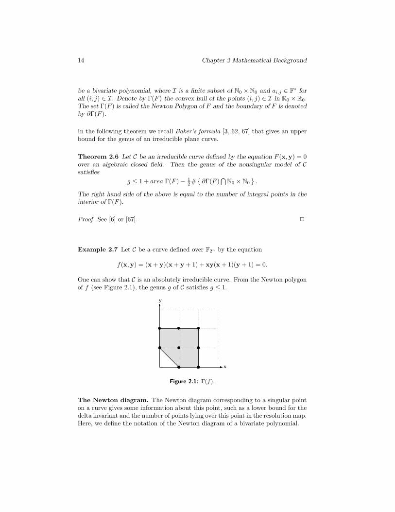
Example 2.7 Let C be a curve defined over F2n by the equation

f(x,y) = (x + y)(x + y + 1) + xy(x + 1)(y + 1) = 0.

One can show that C is an absolutely irreducible curve. From the Newton polygonof f (see Figure 2.1), the genus g of C satisfies g ≤ 1.

x

y

Figure 2.1: Γ(f).

The Newton diagram. The Newton diagram corresponding to a singular pointon a curve gives some information about this point, such as a lower bound for thedelta invariant and the number of points lying over this point in the resolution map.Here, we define the notation of the Newton diagram of a bivariate polynomial.


Definition 2.8 Let F be a field and let

F (x,y) =∑

(i,j)∈I

ai,jxiyj

be a polynomial in two variables, where I is a finite subset of N20 and ai,j ∈ F∗

for all (i, j) ∈ I. Denote by Γ+(F ) the convex hull of the union of the quadrants(i, j) + R2

0 in R20, for all (i, j) ∈ I. The union of the compact edges of Γ+(F )

is denoted by ∂Γ+(F ). Then denote the closure of the set R20 \ Γ+(F ) in R2

0 byΓ−(F ). The boundary of Γ−(F ) is denoted by ∂Γ−(F ). The set Γ−(F ) is calledthe Newton diagram of F .

Remark 2.9 Let C be a reduced plane curve that is defined by an equationF (x,y) = 0 and let P = (0, 0) be a singular point on C. Let Γ−(F ) be theNewton diagram of F . Then δP ≥ νP , where δP is the delta invariant of P andνP is equal to the number of unit-squares with integral vertices, so sets of theform (m,n) + [0, 1]2,m, n ∈ N2

0, contained in the Γ−(F ). For more details see [6,Corollary 3.12].

Definition 2.10 Let γ be a line segment of ∂Γ+(F ) (see Definition 2.8) and letIγ be the set of points on γ and I. Define

Fγ(x,y) =∑

(i,j)∈Iγ

ai,jxiyj .

Remark 2.11 Let C be a reduced plane curve over Fq defined by the equationF (x,y) = 0. Let P = (0, 0) be a singular point on C. Let γ be the line segment of∂Γ+(F ) with endpoints (m1, n1) and (m2, n2). Let m = m2−m1 and n = n1−n2.Define d = gcd(m,n), m′ = m

d and n′ = nd . Then, there exist a unique univariate

polynomial fγ(T ) ∈ F[T ] of degree d such that Fγ(x,y) = xm2yn2fγ(x−m′yn

′).

The number of Fq-rational points on the nonsingular model of C, lying over P inthe resolution map, is at most d and depends on the coefficients of the polynomialFγ or the roots of fγ in F (see [6, Remark 3.16 and 3.18]).

The number of points on a curve. Let C be an absolutely irreducible projectiveplane curve of degree d defined over the finite field Fq.

In case that C is a nonsingular curve with genus g, the well-known Hasse-Weilbound gives the following estimate for the number of Fq-rational points on C.

|#C(Fq)− (q + 1)| ≤ 2g√q. (2.2)

A sharper estimate by Serre [88] is

|#C(Fq)− (q + 1)| ≤ g[2√q ].


In case that C is a singular curve, we consider the resolution of C. For an Fq-rational point P on C, let ϑP be the number of Fq-rational points on C, lying overP in the resolution map ϕ. Then

#C(Fq)−#C(Fq) =∑

P∈C(Fq)

(ϑP − 1).

Let Cs(Fq) be the set of singular points of C(Fq). For a nonsingular point P wehave ϑP = 1. Hence,

#C(Fq)−#C(Fq) =∑

P∈Cs(Fq)

(ϑP − 1).

Example 2.12 Let C be the curve that is defined in Example 2.7. The projectivemodel of C, written C, is defined by the equation

F (X,Y, Z) = (X + Y )(X + Y + Z)Z2 +XY (X + Z)(Y + Z) = 0.

The points P1 = (1 : 0 : 0) and P2 = (0 : 1 : 0), called the points at infinity, are theonly singular points of C. Now, we compute ϑP1 by means of the Newton diagramcorresponding to P1. From the process of dehomogenization with respect to X,we consider the polynomial F1(y, z) = (y + 1)(y + z + 1)z2 + y(z + 1)(y + z).

y

z

Γ+(F1)

Γ−(F1)

Figure 2.2: Γ−(F1), Γ+(F1).

Let γ be the line segment of Diagram 2.2 with endpoints (0, 2) and (2, 0). Then,Fγ(y, z) = y2 + yz + z2 = y2fγ(z/y), where fγ(T ) = T 2 + T + 1 ∈ F2n [T ]. Then,the number of roots of fγ in F2n implies that ϑP1 = 2, if TrF2n/F2(1) = 0, andϑP1 = 0, if TrF2n/F2(1) = 1. Because of the symmetry between x and y, we haveϑP1 = ϑP2 . Therefore, if n is odd, the number of F2n -rational points on C equalsthe number of F2n -rational points on the nonsingular model of C.

2.3 Elliptic curves 17

2.3 Elliptic curves

Now, we briefly review the background on elliptic curves to the extent needed inthis thesis. For a more general presentation of elliptic curves, see [23, 50, 91, 97].

Definition 2.13 A nonsingular absolutely irreducible projective curve definedover F of genus 1 with at least one F-rational point is called an elliptic curveover F.

An elliptic curve E over F can be given by the so-called Weierstrass equation

E : y2 + a1xy + a3y = x3 + a2x2 + a4x + a6, (2.3)

where the coefficients a1, a2, a3, a4, a6 ∈ F. We note that E has to be nonsingular.The set of F-rational points on E, written E(F), is defined by the set of points(x, y) ∈ F× F satisfying Equation 2.3 plus the point at infinity, written P∞. Theset of F-rational points on E by means of the chord-tangent process turns E(F)into an abelian group with P∞ as the neutral element. For finite fields Fq thesubgroups of E(Fq) are used for cryptosystems based on the Discrete Logarithmproblem. The use of elliptic curves in public-key cryptography can offer improvedefficiency and bandwidth.

Let E be a curve defined over F by Equation 2.3. The discriminant of the curveE, denoted by ∆E , satisfies

∆E = −b22b8 − 8b34 − 27b26 + 9b2b4b6,

whereb2 = a2

1 + 4a2, b4 = a1a3 + 2a4,

b6 = a23 + 4a6, b8 = a2

1a6 − a1a3a4 + 4a2a6 + a2a23 − a2

4.

The curve E is nonsingular, and thus is an elliptic curve, if and only if ∆E isnonzero. In this case, the j-invariant of E is defined by j(E) = (b22 − 24b4)3/∆E .If two elliptic curves E1, E2 over F are isomorphic then they have the same j-invariant. Conversely, if j(E1) = j(E2), then E1 and E2 are isomorphic over F.

An elliptic curve E can be defined via the short Weierstrass form. This actuallydepends on the characteristic of the field and on the value of the j-invariant. Allthe cases and equations are summarized in Table 2.1.

There are many other ways to represent an elliptic curve such as Legendre form,Jacobi model, Hessian form, the intersection of two quadratic surfaces and so on(see e.g. [23, Chapter 13] or [97, Chapter 2]). In [36], the explicit formulas aregiven for the number of distinct elliptic curves (up to isomoroprism) in severalfamilies of curves of cryptographic interest.


char(F) Equation ∆E j(E)

6= 2, 3 y2 = x3 + a4x + a6 −16(4a34 + 27a2

6) 1728a34/4∆E

3 y2 = x3 + a4x + a6 −a34 0

3 y2 = x3 + a2x2 + a6 −a32a6 −a3

2/a6

2 y2 + a3y = x3 + a4x + a6 a43 0

2 y2 + xy = x3 + a2x2 + a6 a6 1/a6

Table 2.1: Short Weierstrass equations.

Further, several coordinate systems are proposed to improve the efficiency andthe speed of the addition and doubling formulas in the group of points on ellipticcurves over finite fields (see e.g. [8, 23, 50] and references therein).

2.3.1 Edwards curve

Recently, Edwards [26] introduced a new form for elliptic curves. He showed thatevery elliptic curve over a field F with char(F) 6= 2 is birationally equivalent (in anappropriate sense) to one in the form x2 +y2 = c2(1+x2y2), where c is a constantin F such that c5 6= c. The simple addition law on this form is given by

(x1, y1), (x2, y2) 7→(

x1y2 + y1x2

c(1 + x1x2y1y2),

y1y2 − x1x2

c(1− x1x2y1y2)

).

After that, Bernstein and Lange [9] proposed a slightly generalized form

x2 + y2 = c2(1 + dx2y2),

called Edwards curve, for elliptic curves over F with char(F) 6= 2. The additionlaw on Edwards curve is similar to that of the original Edwards curve. If c and dare nonzero constants in F such that dc4 6= 1, the addition law is given by

(x1, y1), (x2, y2) 7→(

x1y2 + y1x2

c(1 + dx1x2y1y2),

y1y2 − x1x2

c(1− dx1x2y1y2)

).

The point (0, 1) is the neutral element of the addition law. The negative of a pointP = (x1, y1) can be computed by reflecting the x-coordinate across the y-axis:−P = (−x1, y1). The addition law is strongly unified; i.e., the same formulas canalso be used for doubling. If d is not a square then the addition law is complete;i.e., the addition law holds for all inputs.

2.4 Weil descent 19

A sequence of papers [7, 9, 10] showed that, for cryptographic applications, Ed-wards curves involve significantly fewer multiplications than short Weierstrass formcurves in Jacobian coordinates, which so far was considered as the faster system.

In Chapter 8, we generalize the idea of Edwards curve to fields with characteristic 2.

2.4 Weil descent

Weil descent is a well known technique in algebraic geometry. It relates a geometricd-dimensional object over a field K to a nd-dimensional object over a field F, whereK is a field of degree n over F. The use of Weil descent technique is suggested byFrey [38] for cryptographic applications such as DL system.

Here we explain the easiest case. Let K be a field extension of degree n over Fand let {α1, . . . , αn} be a basis of K over F. Let V be an affine variety in Ad(K)defined by the m equations

Fi(x1, . . . ,xd) = 0, for i = 1, . . . ,m,

with Fi ∈ K[x1, . . . ,xd]. Then, we consider dn variables yi,j by xi =∑nj=1 αjyi,j .

We replace the variables xi in the equations defining V by these expressions. Next,we write the coefficients of the resulting relations as F-linear combinations of thebasis {α1, . . . , αn} and order these relations according to this basis. As result weobtain the m equations

Gi(y1,1, . . . ,yd,n) =∑nj=1 αjgi,j(y1,1, . . . ,yd,n) = 0,

where gi,j ∈ F[y1,1, . . . ,yd,n]. The Weil descent of V over F, written WK/F(V ), isdefined by the mn equations

gi,j(y1,1, . . . ,yd,n) = 0, for i = 1, . . . ,m, j = 1, . . . , n.

Example 2.14 Let C be an affine curve over F22` given by the equation

y2 + xy = f(x),

where ` is a positive integer and f is a polynomial in F22` [x]. Consider F22` as aquadratic extension of F2` with a basis {1, t}, where t2 + t+ c = 0 for an elementc ∈ F2` . So, for all x in F2n , we can write x = x0 +x1t, where x0 and x1 are in F2` .Here, we compute the Weil descent WF22`/F2`

(C) of C. We consider the variablesx0, x1, y0 and y1 by x = x0 + x1t and y = y0 + y1t. Then y2 + xy = f(x)becomes

(y0 + y1t)2 + (x0 + x1t)(y0 + y1t) = f(x0 + x1t).

After expansion this is of the form

y20 + cy2

1 + x0y0 + cx1y1 + (y21 + x0y1 + x1y0 + x1y1)t = f0(x0,x1) + f1(x0,x1)t,


where f0 and f1 are in F2` [x0,x1]. Hence, the Weil descent WF22`/F2`(C) of C is

defined by the following system of equations.

{y2

0 + cy21 + x0y0 + cx1y1 + f0(x0,x1) = 0

y21 + x0y1 + x1y0 + x1y1 + f1(x0,x1) = 0.

(2.4)

Note that from a set theoretic point of view WF22`/F2`(C)(F2`) = C(F22`).

2.5 Hyperelliptic curves

Now, we recall the definition of hyperelliptic curves. For a more general back-ground on hyperelliptic curves we refer to [23] and the references therein.

Definition 2.15 An absolutely irreducible nonsingular projective curveH of genusat least 2 is called hyperelliptic if there exists a morphism of degree 2 from H tothe projective line.

The following theorem describes plane singular models of hyperelliptic curves de-fined over Fq.

Theorem 2.16 Let H be a hyperelliptic curve of genus g over Fq. Then, if q isodd, H has a plane model of the form

y2 = f(x),

where f is a square free polynomial in Fq[x] and 2g + 1 ≤ deg(f) ≤ 2g + 2. Theplane model is singular at infinity. If deg(f) = 2g + 1 then the point at infinityramifies and H has only one point at infinity. If deg(f) = 2g+ 2 then H has zeroor two Fq-rational points at infinity.

If q is even, H has a plane model of the form

y2 + h(x)y = f(x),

where h, f are polynomials in Fq[x], f monic and either deg(h) ≤ g, deg(f) = 2g+1or deg(h) = g + 1, deg(f) ≤ 2g + 2. Furthermore, if y2 + h(x)y = f(x) for(x, y) ∈ Fq × Fq, then 2y + h(x) 6= 0 or h′(x)y − f ′(x) 6= 0. The plane modelis singular at infinity. If deg(f) = 2g + 1, deg(h) ≤ g then the point at infinityramifies and H has only one point at infinity. If deg(f) ≤ 2g + 2, deg(h) = g + 1then H has zero or two Fq-rational points at infinity.

Proof. See [2]. 2

2.6 The Jacobian of hyperelliptic curves 21

In this thesis, we concentrate on hyperelliptic curves with exactly one point atinfinity. They are called imaginary hyperelliptic curves.

Definition 2.17 An imaginary hyperelliptic curve H of genus g over Fq is definedby an equation of the form

y2 + h(x)y = f(x),

where h, f ∈ Fq[x], f is monic, deg(f) = 2g + 1, deg(h) ≤ g.

For any subfield F of Fq containing Fq, the set

H(F) = {(x, y) ∈ F× F : y2 + h(x)y = f(x)} ∪ {P∞},

is called the set of F-rational points on H. The point P∞ is called the point atinfinity for H. A point P on H, also written P ∈ H, is a point P ∈ H(Fq). Theopposite of a point P = (x, y) on H is defined by the hyperelliptic involution σas σ(P ) = (x,−h(x)− y) and σ(P∞) = P∞.

2.6 The Jacobian of hyperelliptic curves

For elliptic curves one can take the set of points together with the point at infinityas a group. This is no longer possible for hyperelliptic curves. Instead, a group lawis defined via the set of Fq-rational point of the Jacobian of H over Fq, denotedby J(Fq). One can efficiently compute the sum of two points in the Jacobian of Hover Fq, using the algorithms described in [17, 23, 66]. There are two isomorphicrepresentations of the Jacobian of an imaginary hyperelliptic curve H, namely asthe divisor class group of H and as the ideal class group of the maximal orderin the function field of H. The latter representation is often called Mumfordrepresentation [84].

First, we define the notion of the Jacobian in terms of the divisor class group.Let H be an imaginary hyperelliptic curve defined over Fq. A divisor D on His a formal sum of points on H(Fq), D =

∑P∈H mPP, where the mP ∈ Z are

zero except for a finite number of P ∈ H(Fq). The degree of D is defined bydeg D =

∑P∈H mP . Let F be a subfield of Fq containing Fq. A divisor D is

said to be defined over F, if for all automorphisms ϕ in the Galois group of F,ϕ(D) =

∑P∈H mP ϕ(P ) is equal to D, where ϕ(P ) = (ϕ(x), ϕ(y)) if P = (x, y)

and ϕ(P∞) = P∞.

The set of all divisors on H defined over F, denoted by Div(F), forms an additiveabelian group under the addition rule∑

P∈HmPP +

∑P∈H

nPP =∑P∈H

(mP + nP )P.


The set Div0(F) of all divisors on H of degree zero defined over F is a subgroupof Div(F).

Let F[H] = F[x,y]/(y2 +h(x)y− f(x)) be the coordinate ring of H over F. Thenthe function field of H over F is the field of fractions F(H) of F[H]. For a non-zeroelement R in F[H], the divisor of R is defined by div(R) =

∑P∈H ordP (R)P , where

ordP (R) is the order of vanishing of R at P . For a rational function R = F/G,where F , G ∈ F[H], the divisor of R is defined by div(R) = div(F )−div(G) and iscalled a principal divisor. The group of principal divisors on H over F is denotedby P(F) = {div(R) : R ∈ F(H)}.

Definition 2.18 The divisor class group of H over F is the quotient group

Div0(F)/P(F).

This group is also called Picard group of H.

The Jacobian of H over Fq, denoted by J , is an abelian variety of dimension g.In particular, the set of F-rational points of the Jacobian of H over F, denoted byJ(F) is a group which is isomorphic to the divisor class group of H over F.

For each nontrivial point on the Jacobian of H over F there exists a unique divisorD on H defined over F of the form

D =r∑i=1

Pi − rP∞,

where Pi = (xi, yi) ∈ H(F), Pi 6= P∞ and Pi 6= σ(Pj), for i 6= j, r ≤ g. Such adivisor is called a reduced divisor on H over F. By means of Mumford representa-tion [84], each nontrivial point on J(F) can be uniquely represented by a pair ofpolynomials [u(x), v(x)], u, v ∈ F[x], where u is monic, deg(v) < deg(u) ≤ g andu divides v2 + hv − f . The neutral element of J(F), denoted by O, is representedby [1, 0].

Hasse-Weil Theorem for the Jacobians. Let H be a genus-g hyperellipticcurve defined over a finite field Fq and let J(Fq) be the set of Fq-rational points ofthe Jacobian of H over Fq. The Hasse-Weil Theorem gives bounds on the numberof points on H over Fq (see Equation 2.2). Further, by means of the Hasse-WeilTheorem, we have bounds on the group order of the divisor class group. Thefollowing bounds depend only on the finite field and the genus of the curve:

(√q − 1)2g ≤ #J(Fq) ≤ (

√q + 1)2g.

2.7 Kummer surface 23

2.6.1 On the Jacobian of genus-2 curves

In Chapters 6 and 7, we consider genus-2 imaginary hyperelliptic curves. We nowsummarize the main properties and notions on the Jacobian of these curves.

Let H be an imaginary hyperelliptic curve of genus 2 defined over Fq. Let J(Fq)be the set of Fq-rational points of the Jacobian of H over Fq. We partition J(Fq)as J(Fq) = J0 ∪ J1 ∪ J2, where J0 = {O} and Jr, for r = 1, 2 is defined as

Jr =

{D ∈ J(Fq) : D =

r∑i=1

Pi − rP∞

}.

Let D ∈ J(Fq). Note that φ(D) = D, where φ : Fq −→ Fq is the Frobenius mapdefined by φ(x) = xq and extended to the Jacobian of H as above. Let D haveMumford representation D = [u(x), v(x)], for some u, v ∈ Fq[x]. Then D ∈ Jr ifand only if deg(u) = r and u, v are defined over Fq. We shall explain this in moredetail.

If D ∈ J1, then D = P − P∞, where P 6= P∞ and P = (xP , yP ) ∈ H(Fq).Furthermore, D is represented by [x− xP , yP ].

If D ∈ J2, then D = P1 + P2 − 2P∞ for some points P1, P2, where P1, P2 6= P∞and P1 6= σ(P2). Furthermore, D is represented by [u(x), v(x)], where u(x) =(x − xP1)(x − xP2), v(xP1) = yP1 and v(xP2) = yP2 . There are two possibilitiesfor D:

• First, φ(P1) = P1. Since φ(D) = D, we have φ(P2) = P2. So, P1, P2 ∈H(Fq). Hence, xP1 , xP2 ∈ Fq. So, in this case, u is a reducible polynomialover Fq.

• Secondly, φ(P1) 6= P1. Since φ(D) = D, it follows that φ(P1) = P2 andφ(P2) = P1. So, φ(φ(P1)) = P1, φ(P1) 6= P1 and φ(P1) 6= σ(P1). Hence,P1 ∈ H(Fq2) and xP1 /∈ Fq. If xP1 ∈ Fq, then φ(P1) = (φ(xP1), φ(yP1)) =(xP1 , φ(yP1)), so φ(P1) is equal to either P1 or σ(P1), which is a contradiction.Hence, u is an irreducible polynomial over Fq.

2.7 Kummer surface

Now, we briefly recall the notion of a Kummer surface associated to the Jacobianof genus-2 hyperelliptic curves. For the general background, we refer to [18].

Let H be an imaginary hyperelliptic curve of genus 2 defined over Fq, for odd q.Then H has a plane model of the form

y2 = f(x) = x5 + f4x4 + f3x3 + f2x2 + f1x + f0, (2.5)


where fi ∈ Fq and f is a square-free polynomial. Associated with the curve H,there exists a quartic surface K in P3, called the Kummer surface, which is givenby the equation

A(k1, k2, k3)k24 +B(k1, k2, k3)k4 + C(k1, k2, k3) = 0,

where

A(k1, k2, k3) =k22 − 4k1k3,

B(k1, k2, k3) =− 2(2f0k31 + f1k

21k2 + 2f2k2

1k3 + f3k1k2k3 + 2f4k1k23 + k2k

23),

C(k1, k2, k3) =− 4f0f2k41 + f2

1 k41 − 4f0f3k3

1k2 − 2f1f3k31k3 − 4f0f4k2

1k22

+ 4f0k21k2k3 − 4f1f4k2

1k2k3 + 2f1k21k

23 − 4f2f4k2

1k23 + f2

3 k21k

23

− 4f0k1k32 − 4f1k1k

22k3 − 4f2k1k2k

23 − 2f3k1k

33 + k4

3.

Let J be the Jacobian of H over Fq (see Subsection 2.6.1). Then there exists aparticular map

κ : J(Fq) −→ K(Fq),

where κ(D) = κ(−D), for all D ∈ J(Fq) and κ(O) = (0, 0, 0, 1). This map does notpreserve the group structure, however, it endows a pseudo-group structure uponK (see [18]). In particular, a scalar multiplication on the image of κ is defined by

mκ(D) = κ(mD),

for m ∈ Z and D ∈ J(Fq). Furthermore, the above definition can be extended tohave a scalar multiplication on K, since each point on K can be pulled back to theJacobian of H or to the Jacobian of the quadratic twist of H. So, the Kummersurface K could be used for a Diffie-Hellman key exchange protocol (see [93]).

2.8 A surface related to the Jacobian in odd char-acteristic

In this section we introduce a surface related to the Jacobian of a genus-2 hyperel-liptic curve over a finite field with odd characteristic. The result of this section willbe used as mathematical background for the proofs of main theorems in Chapter 6.

LetH be an imaginary genus-2 hyperelliptic curve over Fq, where q is odd. ThenHhas a plane model of the form

y2 = f(x) =5∏i=1

(x− λi), (2.6)

2.8 A surface related to the Jacobian in odd characteristic 25

where the λi’s are pairwise distinct elements of Fq. Let J(Fq) be the set of Fq-rational points of the Jacobian of H over Fq (see Subsection 2.6.1). The neutralelement of J(Fq) is denoted by O. Let Ht be a quadratic twist of H that has aplane model of the form

αy2 = f(x), (2.7)

where α is a non-square element of Fq. Let J t be the Jacobian of Ht over Fq.

We define the bivariate polynomial Φ ∈ Fq[x1,x2] by

Φ(x1,x2) = f(x1)f(x2).

Clearly, Φ is a symmetric polynomial. From Equation (2.6), we obtain

Φ(x1,x2) =5∏i=1

(x1 − λi)(x2 − λi) =5∏i=1

(x1x2 − λi(x1 + x2) + λ2i ).

We define the bivariate polynomial Ψ in Fq[a,b] by

Ψ(a,b) =5∏i=1

(b− λia + λ2i ). (2.8)

Definition 2.19 Let R be the affine surface defined over Fq by the equation

z2 = Ψ(a,b).

Let S2 be the symmetric group acting on {1, 2}. It acts in a natural way on H×H.Then, one can see that R = (H ×H)/(〈(σ, σ)〉 × S2), where σ is the hyperellipticinvolution. The surface R is almost the same as the Kummer surface K associatedto the Jacobian of H.

Remark 2.20 Let D ∈ J(Fq) be represented by D = P1 + P2 − 2P∞, whereP1, P2 ∈ H(Fq), P1, P2 6= P∞ and P1 6= σ(P2). Then, y2

P1= f(xP1) and y2

P2=

f(xP2). Let z = yP1yP2 . Then, z2 = Φ(xP1 , xP2). Let a = xP1 + xP2 , b = xP1xP2 .Then z2 = Ψ(a, b). This means that (a, b, z) is a point of R. Furthermore,(a, b, z) ∈ R(Fq).

Remark 2.21 Let D ∈ J t(Fq) be represented by D = P1 + P2 − 2P∞, whereP1, P2 are points on Ht(Fq), P1, P2 6= P∞ and P1 6= σ(P2). So, αy2

P1= f(xP1) and

αy2P2

= f(xP2). Let z = αyP1yP2 . Then z2 = Φ(xP1 , xP2). Let a = xP1 + xP2 , b =xP1xP2 . Then z2 = Ψ(a, b) and hence (a, b, z) ∈ R(Fq).


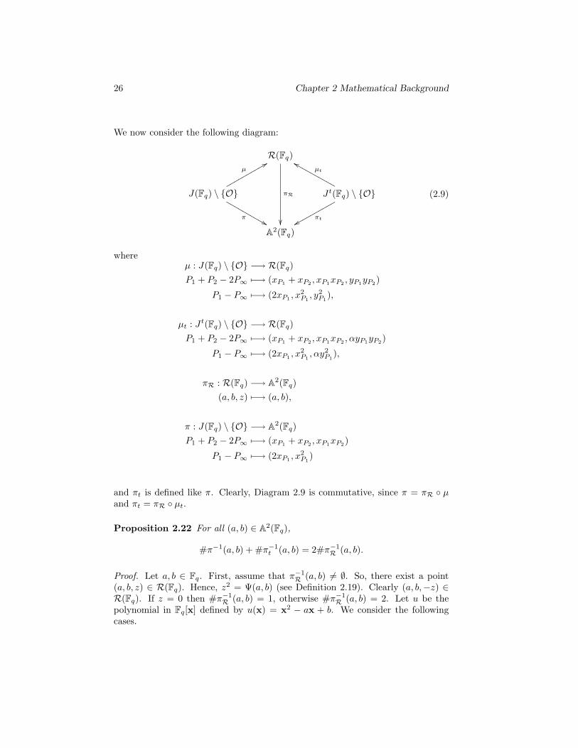
We now consider the following diagram:

R(Fq)

πR

��

J(Fq) \ {O}

µ88qqqqqqqqqq

π&&MMMMMMMMMM

J t(Fq) \ {O}

µt

ffMMMMMMMMMM

πtxxqqqqqqqqqq

A2(Fq)

(2.9)

whereµ : J(Fq) \ {O} −→ R(Fq)P1 + P2 − 2P∞ 7−→ (xP1 + xP2 , xP1xP2 , yP1yP2)

P1 − P∞ 7−→ (2xP1 , x2P1, y2P1

),

µt : J t(Fq) \ {O} −→ R(Fq)P1 + P2 − 2P∞ 7−→ (xP1 + xP2 , xP1xP2 , αyP1yP2)

P1 − P∞ 7−→ (2xP1 , x2P1, αy2

P1),

πR : R(Fq) −→ A2(Fq)(a, b, z) 7−→ (a, b),

π : J(Fq) \ {O} −→ A2(Fq)P1 + P2 − 2P∞ 7−→ (xP1 + xP2 , xP1xP2)

P1 − P∞ 7−→ (2xP1 , x2P1

)

and πt is defined like π. Clearly, Diagram 2.9 is commutative, since π = πR ◦ µand πt = πR ◦ µt.

Proposition 2.22 For all (a, b) ∈ A2(Fq),

#π−1(a, b) + #π−1t (a, b) = 2#π−1

R (a, b).

Proof. Let a, b ∈ Fq. First, assume that π−1R (a, b) 6= ∅. So, there exist a point

(a, b, z) ∈ R(Fq). Hence, z2 = Ψ(a, b) (see Definition 2.19). Clearly (a, b,−z) ∈R(Fq). If z = 0 then #π−1

R (a, b) = 1, otherwise #π−1R (a, b) = 2. Let u be the

polynomial in Fq[x] defined by u(x) = x2 − ax + b. We consider the followingcases.

2.8 A surface related to the Jacobian in odd characteristic 27

1. Assume that u has two distinct roots x1, x2 in Fq. Then there exist y1, y2 ∈Fq, such that P1 = (x1, y1), P2 = (x2, y2) are points either on H(Fq) or onHt(Fq). Indeed, f(x1)f(x2) = Ψ(a, b) = z2, since a = x1 + x2 and b = x1x2.We distinguish two possibilities.

(a) Suppose z 6= 0. Without loss of generality, let P1 ∈ H(Fq). So, y21 =

f(x1). Since f(x1)f(x2) = z2 6= 0, it follows that f(x2) is a squarein Fq. Hence P2 ∈ H(Fq). Note that P1 6= P2, P1 6= σ(P2), P1 6= σ(P1)and P2 6= σ(P2), because x1 6= x2 and y1, y2 6= 0. So, P1, P2 /∈ Ht(Fq).Further, the divisors P1 + P2 − 2P∞ and σ(P1) + σ(P2)− 2P∞ are theonly points of π−1(a, b). Therefore #π−1(a, b) = 4 and #π−1

t (a, b) = 0.

(b) Suppose z = 0. So f(x1)f(x2) = 0. Without loss of generality, letf(x1) = 0. Then P1 is a common point of H(Fq) and Ht(Fq). Thisimplies that P1 = σ(P1). We can assume P2 ∈ H(Fq). If f(x2) 6= 0,then P2 6= σ(P2) and P2 /∈ Ht(Fq). Hence the divisors P1 + P2 − 2P∞and P1+σ(P2)−2P∞ are the only points of π−1(a, b). So #π−1(a, b) = 2and #π−1

t (a, b) = 0. If f(x2) = 0, then P2 = σ(P2) and P2 ∈ Ht(Fq).Therefore the divisor P1 + P2 − 2P∞ is the only point of π−1(a, b) andπ−1t (a, b). So #π−1(a, b) = #π−1

t (a, b) = 1.

2. Assume u has one double root x1 in Fq. Then there exists y1 ∈ Fq, suchthat P1 = (x1, y1) and P1 is a point of H(Fq) or Ht(Fq). Furthermore,(f(x1))2 = Ψ(a, b) = z2, since a = 2x1 and b = x2

1. We consider twopossibilities.

(a) Suppose z 6= 0. So f(x1) 6= 0, i.e. P1 6= σ(P1). Without loss ofgenerality, assume P1 ∈ H(Fq). So P1 /∈ Ht(Fq). Then, the divisors2P1 − 2P∞, 2σ(P1) − 2P∞, P1 − P∞ and σ(P1) − P∞ are the onlypoints of π−1(a, b). Hence, #π−1(a, b) = 4. Also #π−1

t (a, b) = 0, sinceP1, σ(P1) /∈ Ht(Fq).

(b) Suppose z = 0. So f(x1) = 0. Then P1 = σ(P1) and P1 is a commonpoint of H(Fq) and Ht(Fq). Hence, the divisor P1−P∞ is the only pointof π−1(a, b) and π−1

t (a, b). Therefore, #π−1(a, b) = #π−1t (a, b) = 1.

3. Assume u has no root in Fq. Let x1, xq1 be the distinct roots of u in Fq2 . From

the definition of Ψ (see Equation (2.8)), we have f(x1)f(xq1) = Ψ(a, b) = z2,since a = x1 + xq1, b = x1x

q1. Then, NFq2/Fq

(f(x1)) = f(x1)f(xq1) = z2 ∈ Fq.From Lemma 2.1, f(x1) is a square in Fq2 . So there exists y1 ∈ Fq2 suchthat y2

1 = f(x1). Let P1 = (x1, y1), so φ(P1) = (xq1, yq1). Indeed, P1 and

φ(P1) are points of H(Fq2).

Let β be a square root of α in Fq2 . Then Q1 = (x1,y1β ) and φ(Q1) =

(xq1,−yq1β ) are points of Ht(Fq2). Then, we distinguish the following possibil-

ities.


(a) Suppose z 6= 0. So f(x1), f(x2) 6= 0, i.e. y1, y2 6= 0. Thus P1 6= σ(P1),φ(P1) 6= σ(φ(P1)), Q1 6= σ(Q1) and φ(Q1) 6= σ(φ(Q1)). Therefore

π−1(a, b) = {P1 + φ(P1)− 2P∞, σ(P1) + σ(φ(P1))− 2P∞} ,

π−1t (a, b) = {Q1 + φ(Q1)− 2P∞, σ(Q1) + σ(φ(Q1))− 2P∞} .

Hence #π−1(a, b) = #π−1t (a, b) = 2.

(b) Suppose z = 0. Then f(x1) = f(xq1) = 0, i.e., y1 = y2 = 0. So,P1 = σ(P1) and φ(P1) = σ(φ(P1)). Hence, P1 +φ(P1) is the only pointof π−1(a, b). Likewise, Q1 = P1 and P1 + φ(P1) is also the only pointof π−1

t (a, b). Hence #π−1(a, b) = π−1t (a, b) = 1.

Now, assume that π−1R (a, b) = ∅. Then #π−1(a, b) = #π−1

t (a, b) = 0, since Dia-gram 2.9 is commutative (see Remarks 2.20 and 2.21). Therefore, the proof of thisproposition is complete. 2

Theorem 2.23#J(Fq) + #J t(Fq) = 2#R(Fq) + 2.

Proof. We consider the projection maps π, πt and πR in Diagram 2.9. FromProposition 2.22, we have

#J(Fq) + #J t(Fq) = 2 +∑

(a,b)∈A2(Fq)

#π−1(a, b) + #π−1t (a, b)

= 2 +∑

(a,b)∈A2(Fq)

2#π−1R (a, b)

= 2 + 2#R(Fq).

2

2.9 A surface related to the binary Jacobian

Now, we extend the result of Section 2.8 to the Jacobians of genus-2 hyperellipticcurves over binary finite fields. This section gives the mathematical backgroundfor the proofs of the main theorems in Chapter 7.

Let H be an imaginary hyperelliptic curve of genus 2 over Fq, with q = 2n, definedby an equation of the form

y2 + h(x)y = f(x),

2.9 A surface related to the binary Jacobian 29

where h = h2x2 + h1x + h0 and f = x5 + f4x4 + f3x3 + f2x2 + f1x + f0. LetJ(Fq) be the set of Fq-rational points of the Jacobian of H over Fq. Let O be theneutral element of J(Fq).

Let α ∈ Fq with TrFq/F2(α) = 1. Then, there exist an element β ∈ Fq2 \ Fq suchthat β2 + β = α. Let Ht be a projective curve with a plane model of the form

y2 + h(x)y = f(x) + αh2(x). (2.10)

The identification (x,y) −→ (x,y + βh(x)) shows that Ht is isomorphic to Hover Fq2 . Moreover, theses curves are not isomorphic over Fq. This means Ht is aquadratic twist of H. Let J t be the Jacobian of Ht over Fq.

Remark 2.24 For a point P = (x, y) ∈ H(Fq), we have σ(P ) = (x, y + h(x)).For P∞, the point at infinity of H, we have σ(P∞) = P∞. Let

IH = {P ∈ H(Fq) : P = σ(P )}.

Clearly P ∈ IH if and only if P = P∞ or h(x) = 0. These points of IH are exactlythose which correspond to points on both, H(Fq) and Ht(Fq).

Let ν and ω be the polynomials in Fq[x1,x2] defined by

ν(x1,x2) = h(x1)h(x2),

ω(x1,x2) = f(x1)h2(x2) + f(x2)h2(x1).

Clearly, ν and ω are symmetric polynomials. Consider the bivariate polynomialsθ, ψ ∈ Fq[a,b] such that

θ(x1 + x2,x1x2) = ν(x1,x2), ψ(x1 + x2,x1x2) = ω(x1,x2).

Definition 2.25 Let X be the affine surface defined over Fq by the equation

F (a,b, z) = z2 + θ(a,b)z + ψ(a,b) = 0.

Remark 2.26 Let D = P1 +P2− 2P∞ be a divisor of J(Fq), where P1 = (x1, y1)and P2 = (x2, y2) are points on H(Fq), P1, P2 6= P∞ and P1 6= σ(P2). Hence,y21 + h(x1)y1 = f(x1) and y2

2 + h(x2)y2 = f(x2). Let z = h(x1)y2 + h(x2)y1. Thenz2+ν(x1, x2)z = ω(x1, x2). Let a = x1+x2, b = x1x2. Then z2+θ(a, b)z = ψ(a, b).This means that (a, b, z) is a point of X . In fact (a, b, z) ∈ X (Fq), since a, b, z ∈ Fq.

Remark 2.27 Let D = P1 +P2−2P∞ be a divisor of J t(Fq), where P1 = (x1, y1)and P2 = (x2, y2) are points on Ht(Fq), P1, P2 6= P∞ and P1 6= σ(P2). Let z =h(x1)y2 +h(x2)y1. Similarly to Remark 2.26, one can show that (x1 +x2, x1x2, z)is a point of X (Fq).


Following Remarks 2.26 and 2.27, we consider the diagram

X (Fq)

πX

��

J(Fq) \ {O}

µ88qqqqqqqqqq

π&&MMMMMMMMMM

J t(Fq) \ {O}

µt

ffMMMMMMMMMM

πtxxqqqqqqqqqq

A2(Fq)

(2.11)

where

µ : J(Fq) \ {O} −→ R(Fq)P1 + P2 − 2P∞ 7−→ (xP1 + xP2 , xP1xP2 , h(xP1)yP2 + h(xP2)yP1)

P1 − P∞ 7−→ (0, x2P1, 0),

πX : X (Fq) −→ A2(Fq)(a, b, z) 7−→ (a, b),

π : J(Fq) \ {O} −→ A2(Fq)P1 + P2 − 2P∞ 7−→ (xP1 + xP2 , xP1xP2)

P1 − P∞ 7−→ (0, x2P1

)

and µt, πt are defined respectively similar to µ, π. Clearly, Diagram 2.11 iscommutative, since π = πX ◦ µ and πt = πX ◦ µt.

Proposition 2.28 For all (a, b) ∈ A2(Fq),

#π−1(a, b) + #π−1t (a, b) = 2#π−1

X (a, b).

Proof. Let a, b ∈ Fq. First, assume that π−1(a, b) 6= ∅. So, there exist apoint (a, b, z) ∈ X (Fq). Hence z2 + θ(a, b)z + ψ(a, b) = 0 (see Definition 2.25).Also (a, b, z + θ(a, b)) ∈ X (Fq). If θ(a, b) = 0 then #π−1

X (a, b) = 1, otherwise#π−1

X (a, b) = 2. Let u be the polynomial in Fq[x] defined by u(x) = x2 + ax + b.We consider the following cases.

1. Assume u has two distinct roots x1, x2 in Fq. Then there exist y1, y2 ∈ Fq,such that P1 = (x1, y1), P2 = (x2, y2) are points either on H(Fq) or onHτ (Fq). Furthermore, θ(a, b) = h(x1)h(x2) and ψ(a, b) = f(x1)h2(x2) +f(x2)h2(x1), because a = x1+x2 and b = x1x2. We distinguish the followingpossibilities.

2.9 A surface related to the binary Jacobian 31

(a) Suppose θ(a, b) 6= 0. So, h(x1), h(x2) 6= 0. Without loss of generality,let P1 ∈ H(Fq). We note that

TrFq/F2(ψ(a,b)θ2(a,b) ) =TrFq/F2(

f(x1)h2(x2)+f(x2)h

2(x1)h2(x1)h2(x2)

)

=TrFq/F2(f(x1)h2(x1)

) + TrFq/F2(f(x2)h2(x2)

).

So TrFq/F2(f(x2)h2(x2)

) = 0, since TrFq/F2(ψ(a,b)θ2(a,b) ) = TrFq/F2(

f(x1)h2(x1)

) = 0.Hence P2 ∈ H(Fq). Indeed, P1, P2 /∈ Ht(Fq), since h(x1), h(x2) 6= 0(see Remark 2.24). Furthermore, P1 6= P2, P1 6= σ(P2), P1 6= σ(P1)and P2 6= σ(P2). Hence, the divisors P1 +P2−2P∞, P1 +σ(P2)−2P∞,σ(P1) + P2 − 2P∞ and σ(P1) + σ(P2) − 2P∞ are the only points ofπ−1(a, b). So, #π−1(a, b) = 4 and #π−1

t (a, b) = 0.(b) Suppose θ(a, b) = 0. So h(x1)h(x2) = 0. Without loss of generality,

let h(x1) = 0. Then P1 is a common point of H(Fq) and Ht(Fq) (seeRemark 2.24). This implies that P1 = σ(P1). We may assume P2 ∈H(Fq). If h(x2) 6= 0, then P2 6= σ(P2) and P2 /∈ Ht(Fq). Hence thedivisors P1 + P2 − 2P∞ and P1 + σ(P2) − 2P∞ are the only pointsof π−1(a, b). So #π−1(a, b) = 2 and #π−1

t (a, b) = 0. If h(x2) = 0,then P2 = σ(P2) and P2 ∈ Ht(Fq). Hence, the divisor P1 + P2 − 2P∞is the only point of π−1(a, b) and π−1

t (a, b). Therefore, #π−1(a, b) =#π−1

t (a, b) = 1.

2. Assume u has a double root x1 in Fq. Then there exists y1 ∈ Fq, such thatP1 = (x1, y1) is a point of H(Fq) or Ht(Fq). Furthermore, θ(a, b) = h2(x1)and ψ(a, b) = 0, because a = 0 and b = x2

1. We distinguish two possibilities:

(a) Suppose θ(a, b) 6= 0. So h(x1) 6= 0. Without loss of generality, weassume P1 ∈ H(Fq). Then P1 /∈ Ht(Fq), since h(x1) 6= 0. This impliesthat P1 6= σ(P1). So, the divisors 2P1 − 2P∞, 2σ(P1)− 2P∞, P1 − P∞and σ(P1)−P∞ are the only points of π−1(a, b). Hence #π−1(a, b) = 4.Also #π−1

t (a, b) = 0, since P1, σ(P1) /∈ Ht(Fq).(b) Suppose θ(a, b) = 0. So h(x1) = 0. Then P1 = σ(P1) and P1 is a

common point of H(Fq) and Ht(Fq). So, the divisor P1−P∞ is the onlypoint of π−1(a, b) and π−1

t (a, b). Hence #π−1(a, b) = #π−1t (a, b) = 1.

3. Assume u has no root in Fq. Let x1, xq1 be the roots of u in Fq2 . It follows

from the definitions of θ and ψ that θ(a, b) = h(x1)h(xq1) and ψ(a, b) =

f(x1)h2(xq1) + f(xq1)h2(x1). We distinguish the following possibilities.

(a) Suppose θ(a, b) 6= 0. Then h(x1), h(xq1) 6= 0. We note that

TrFq2/F2(f(x1)h2(x1)

) =TrFq/F2(TrFq2/Fq( f(x1)h2(x1)

))

=TrFq/F2(f(x1)h2(x1)

+ f(xq1)

h2(xq1)

)

=TrFq/F2(ψ(a,b)θ2(a,b) ) = 0.


Then there exists y1 ∈ Fq2 such that P1 = (x1, y1) ∈ H(Fq2). Alsoφ(P1) = (xq1, y

q1) ∈ H(Fq2). Let β ∈ Fq2 such that β2 + β = α. Then

Q1 = (x1, y1 + βh(x1)) and φ(Q1) = (xq1, yq1 + (β + 1)h(xq1)) are points

of Ht(Fq2). One sees that P1 6= σ(P1), φ(P1) 6= σ(φ(P1)), Q1 6= σ(Q1)and φ(Q1) 6= σ(φ(Q1)). Therefore

π−1(a, b) = {P1 + φ(P1)− 2P∞, σ(P1) + σ(φ(P1))− 2P∞} ,

π−1t (a, b) = {Q1 + φ(Q1)− 2P∞, σ(Q1) + σ(φ(Q1))− 2P∞} .

So #π−1(a, b) = #π−1t (a, b) = 2.

(b) Suppose θ(a, b) = 0. So, h(x1) = h(xq1) = 0. Thus P1 = (x1,√f(x1)) ∈

H(Fq2) and φ(P1) = (xq1,√f(xq1)) ∈ H(Fq2). Furthermore, P1 = σ(P1)

and φ(P1) = σ(φ(P1)). Also P1, φ(P1) ∈ Ht(Fq2). Therefore, P1 +φ(P1) is the only point of π−1(a, b) and π−1

t (a, b). Hence, #π−1(a, b) =π−1t (a, b) = 1.

Now, assume that π−1R (a, b) = ∅. Then #π−1(a, b) = #π−1

t (a, b) = 0, since Di-agram 2.11 is commutative (see Remarks 2.26 and 2.27). So, the proof of thisproposition is complete. 2

Theorem 2.29#J(Fq) + #J t(Fq) = 2#X (Fq) + 2.

Proof. Proposition 2.28 concludes the proof of this theorem. 2

2.10 Deterministic extractor

Here, we define the notion of a deterministic extractor and a quality measure calledstatistical distance. For a general definition of extractors we refer to [89, 96].

Definition 2.30 Let X and Y be S-valued random variables, where S is a finiteset. Then the statistical distance ∆(X,Y ) of X and Y is

∆(X,Y ) = 12

∑s∈S |Pr[X = s]− Pr[Y = s] | .

Let US denote a random variable uniformly distributed on S. We say that anS-valued random variable X is δ-uniform, if ∆(X,US) ≤ δ.

2.10 Deterministic extractor 33

Note that if the random variable X is δ-uniform, then no algorithm can distinguishX from US with advantage larger than δ, that is, for all algorithmsD : S −→ {0, 1}

|Pr[D(X) = 1]− Pr[D(US) = 1]| ≤ δ.

See [78].

Definition 2.31 Let S, T be finite sets. Consider a function Ext : S −→ T . Wesay that Ext is a deterministic (T, δ)-extractor for S if Ext(US) is δ-uniform onT . That is

∆(Ext(US), UT ) ≤ δ.

In the case that T = {0, 1}k, we say that Ext is a (k, δ)-deterministic extractorfor S.

In Chapters 4, 5, 6 and 7, we consider deterministic (Fq, δ)-extractors, where q isa prime power. Observe that converting random elements of Fq into random bitstrings is a relatively easy problem. For instance, one can represent an element ofFq by a number in Zq and convert this number to a bit-string of a length equal orvery close to the bit length of q (e.g. see [60]). Furthermore, if q is close to a powerof 2, that is, 0 ≤ (2n − q)/2n ≤ δ for a small δ, then the bit-string representationof the uniform element UFq

is statistically close to n uniformly random bits. Thefollowing simple lemma is a well-known result (the proof can be found, for instance,in [20]).

Lemma 2.32 Let bits : Fq −→ {0, 1}n be a bit-representation function for Fq.Suppose 0 ≤ (2n − q)/2n ≤ δ. Then bits is an (n, δ)-deterministic extractor.

2.10.1 Extractor for a subgroup

One application of extractors is to extract bits from a shared secret element in thefinal step of key exchange protocols, e.g. the Diffie-Hellman key exchange protocol.It is assumed that this group element is uniformly distributed if the DecisionalDiffie-Hellman problem (DDH) in this group is believed as a hard problem.

We note that, if the order of the group is divisible by a small number, the DDHproblem in the corresponding group is easy. In this case, the main subgroup issuggested for cryptographic applications. Further, the DDH problem in the mainsubgroup is assumed to be intractable.

Let A be an additive group of order 2m, where m is odd. Let G be the mainsubgroup of A of order m. If we have an extractor for A with some additionalrequirement, then we can propose an extractor for the main subgroup G.


Let 0 be the neutral element of A and t be the element of order 2. Let β be a bitdistinguishing a from −a satisfying

β : A→ {0, 1},β(a) = 0, if a = −a,β(a) + β(−a) = 1, if a 6= −a.

Let Ext be a deterministic (T, δ)-extractor for A, for some T and δ. SupposeExt(a) = Ext(−a) for all a ∈ A. Furthermore, assume Ext(0) = Ext(t). Wepropose an extractor ext for G as a modified version of Ext. The extractor ext isdefined by the function

ext : G→ T,

ext(a) = Ext(a+ β(a)t).

Proposition 2.33 Let z ∈ T . Then

#Ext−1(z) = 2#ext−1(z).

Proof. We consider the map ξ : Ext−1(z) −→ ext−1(z) defined by

ξ(a) =

a, if a ∈ G, β(a) = 0,− a, if a ∈ G, β(a) = 1,− a+ t, if a /∈ G, β(a+ t) = 0,a+ t, if a /∈ G, β(a+ t) = 1.

The map ξ is surjective. Indeed it is a 2 : 1 map, since Ext(a) = Ext(−a) for alla ∈ A and Ext(0) = Ext(t). 2

Proposition 2.34 Ext is a (T, δ)-deterministic extractor for A if and only if extis a (T, δ)-deterministic extractor for G.

Proof. Let XA and XG be the T -valued random variables that are defined by

XA = Ext(a), for a ∈R A and XG = ext(a), for a ∈R G.

Let z ∈ T . Proposition 2.33 now implies

Pr[XA = z] =#Ext−1(z)

#A=

#ext−1(z)#G

= Pr[XG = z].

Hence ∆(XA, UT ) = ∆(XG, UT ), for the uniform random variable UT in T . 2

2.11 Deterministic extractors for varieties 35

2.11 Deterministic extractors for varieties

In this section, we describe a simple way to construct an extractor based on curves,Jacobians and in general varieties over finite fields.

Let A be a variety of dimension n defined over a finite field Fq. Consider afinite map from the variety A to the affine space of dimension n, i.e., a Noethernormalization of the variety A (see [27]). Such a map always exists, but it isnot unique. So, in general, we can assume that each point P of A(Fq) has acompressed representation by n coordinates (x1, . . . , xn), where xi ∈ Fq. Wenote that this representation does not uniquely determine points on A, extracoordinates are necessary to represent a point uniquely. On the other hand, foreach choice (x1, . . . , xn) ∈ Fnq , there exist only finitely many points on A. Assumethat each point belongs to no more than e points on A.

For example, if A is a (hyper)elliptic curve in Weierstrass form, we can considerthe x-coordinate of the point as a compact representation. In the case where A isthe Jacobian of a hyperelliptic curve, we can compactly represent each point bythe coefficients of the first polynomial in Mumford representation.

We can define a deterministic extractor, based on A, that for a given point P onA outputs some fixed coordinates of the compact representation of P .

Definition 2.35 Let A be a variety of dimension n and degree d defined overa finite field Fq. Suppose each point P of A has a compressed representation(x1, x2, . . . , xn), where xi ∈ Fq. Let k be a positive integer less than or equal ton. Fix numbers i1, i2, . . . , ik, such that 1 ≤ i1 < i2 < . . . < ik ≤ n. The extractorExti1,i2,...,ik for A is defined as

Exti1,i2,...,ik : A(Fq) −→ FkqExti1,i2,...,ik(P ) = (xi1 , xi2 , . . . , xik).

In the following, we give some examples of the extractor Exti1,i2,...,ik based oncurves and the Jacobians.

Example 2.36 Consider the finite field Fqn , where q is a prime power and n isa positive integer. Let {α1, α2, . . . , αn} be a basis of Fqn over Fq. Let C be anabsolutely irreducible curve defined over Fqn by the equation f(x,y) = 0, wheref ∈ Fqn [x,y]. By means of the Weil descent technique (see Section 2.4), wedefine A as WFqn/Fq

(C). So, A is a variety of dimension n. Furthermore, a pointP = (x, y) on C(Fqn) has a compressed representation (x1, . . . , xn) ∈ Fnq , wherex = x1α1 + x2α2 + . . .+ xnαn. Now, Definition 2.35 defines extractor for C.

Example 2.37 Let H be an imaginary hyperelliptic curve defined over Fq ofgenus n. Here, we let A = J be the Jacobian of H over Fq. We note that A is a


variety of dimension n over Fq. A point P on A(Fq) has Mumford representation[u(x), v(x)], where u, v ∈ Fq[x] and u is monic of degree d less than or equal to n(see Section 2.6). The point P has a compressed representation (u0, u1, . . . , un−1),where u(x) = xd + ud−1xd−1 + . . .+ u1x + u0 and ui = 0, for d ≤ i ≤ n− 1. Now,Definition 2.35 suggests the extractor Ext based on the Jacobian of H over Fq.

Analysis of the extractor. Now, we investigate the distribution of the outputExti1,i2,...,ik(P ), where points P are chosen uniformly at random in A. Fix k andsome 1 ≤ i1 < i2 < . . . < ik ≤ n. In the following we abbreviate Exti1,i2,...,ik(P )by Extk.

Let UFkq

be a uniform random variable and let X be an Fkq -valued random variabledefined by

X = Extk(P ), for P ∈R A(Fq).

Let a ∈ Fkq . The uniform random variable UFkq

satisfies Pr[UFkq

= a] = 1/qk.

For the Fkq -valued random variable X we have Pr[X = a] = #Ext−1k (a)

#A(Fq) . In thefollowing, we compute the statistical distance between the random variable X andthe uniform random variable UFk

q.

∆(X,UFkq) =

12

∑a∈Fk

q

∣∣∣Pr[X = a]− Pr[UFkq

= a]∣∣∣ =

12

∑a∈Fk

q

∣∣∣∣#Ext−1k (a)

#A(Fq)− 1qk

∣∣∣∣ .From the Lang-Weil Theorem, we can consider a bound on the number of pointson A as

|#A(Fq)− qn| ≤ Aqn−12 ,

where A is a constant in terms of the parameters of A such as the degree and thedimension of A. The fibers of Extk are generally varieties of dimension n− k, butthere are exceptional fibers which are reducible. It is necessary to distinguish thereducible fibers, so let IExtk

={a ∈ Fkq : Ext−1

k (a) is reducible}. Then, by means

of the Lang-Weil Theorem, we obtain a number B such that the following boundis satisfied for all fibers Ext−1

k (a), where a /∈ IExtk.∣∣#Ext−1

k (a)(Fq)− qn−k∣∣ ≤ Bqn−k−

12 .

Further, for all a ∈ IExtk, we can consider a trivial bound

0 ≤ #Ext−1k (a)(Fq) ≤ eqn−k.

Hence,

∆(X,UFkq) =

∑a∈IExtk

∣∣qk#Ext−1k (a)−#A(Fq)

∣∣2qk#A(Fq)

+∑

a∈Fkq\IExtk

∣∣qk#Ext−1k (a)−#A(Fq)

∣∣2qk#A(Fq)

.

2.11 Deterministic extractors for varieties 37

Let w = #IExtk. Then

∆(X,UFkq) ≤ ((e− 1)qn +Aqn−

12 )w + (A+B)qn−

12 (qk − w)

2qk(qn −Aqn−12 )

=((e− 1)

√q −B)w + (A+B)qk

2qk(√q −A)

=A+B

2 + ε(q)√q

,

where ε(q) = A(A+B)+((e−1)√q−B)wq−k+ 1

2

2(√q−A) . In the case that w = 0, ε(q) < 1, for

q ≥ A2(A+B+2)2

4 .

For an accurate analysis of the extractor, it is necessary to have proper boundson the number of points on fibres of Extk. This means, a detailed study on thegeometry of the fibers of Extk is required. Further, some counting techniques areneeded to find tight estimates for the number of points on the fibres. Clearly,the analysis will be more precise, if we consider extractors based on particularfamilies of varieties. For example, the analysis of the proposed extractor Extkfor the families of curves and Jacobians given by Examples 2.36 and 2.37, will bemore precise that in general. In this thesis we concentrate of some families givenby these examples.

The following example presents an extractor for an affine curve C. Provided thatthe point P is chosen uniformly at random in C, the bits extracted from the pointP are uniformly distributed.

Example 2.38 Consider the finite field F2k , where k is odd. So, every elementy ∈ F2k can be represented by (y1, y2, . . . , yk), where yi ∈ {0, 1}. Let C be theaffine model of an elliptic curve over F2k defined by the equation

y2 + y = x3 + b,

where b ∈ F2k . We define an extractor ext for the curve C by the function:

ext : C(F2k) −→ {0, 1}k

ext(x, y) = (y1, y2, . . . , yk).

Then, ext is a (k, 0)-deterministic extractor for C, because ext is a bijection.

Chapter 3

Norm and Trace Varieties

In this chapter, we describe two scalar restriction techniques for the families ofKummer and Artin-Schreier curves. These techniques enable us to associate acurve from these families defined over Fqn to an n-dimensional affine hypersurfacedefined over Fq.

Let C be an absolutely irreducible smooth Kummer curve defined by ym = f(x),where f is a polynomial in Fqn [x] and m is a positive integer dividing q − 1.The norm variety N is an n-dimensional hypersurface over Fq related to thecurve C. An Fqn-rational point (x, y) on C is mapped to an Fq-rational point(x1, x2, . . . , xn, z) on N , where x ∈ Fqn is represented by (x1, x2, . . . , xn) in Fnqand z equals the norm of y over Fq. This map is m : 1 for points (x, y) with y 6= 0and 1 : 1 for points (x, y) with y = 0. Theorem 3.7 will show that the number ofFqn-rational points of C equals the number of Fq-rational points of N .

A similar idea can be applied to an absolutely irreducible smooth curve X in theArtin-Schreier form yp − y = F (x), where F is a rational function in Fqn(x) andp is the characteristic of the field Fq. The curve X over Fqn is related to the tracevariety which is an n-dimensional hypersurface T over Fq. The corresponding map

The result of this chapter is based on: R. R. Farashahi. Norm and Trace Varieties. preprint,2008. Moreover, other proofs of Theorems 3.7 and 3.13 are presented by B. Edixhoven in theappendix of the latter. The idea of Section 3.1 is based on: R. R. Farashahi and R. Pellikaan, TheQuadratic Extension Extractor for (Hyper)Elliptic Curves in Odd Characteristic. In Interna-tional Workshop on the Arithmetic of Finite Fields–WAIFI 2007, volume 4547 of Lecture Notesin Computer Science, pages 219–236. Springer-Verlag, 2007. The result of Subsection 3.2.1is based on: R. R. Farashahi and R. Pellikaan, and A. Sidorenko, Extractors for Binary El-liptic Curves. In Designs, Codes and Cryptography, 49(1–3):171–186, 2008. Open access athttp://www.springerlink.com/content/lm35kv103x34j754.

40 Chapter 3 Norm and Trace Varieties

assigns an Fqn -rational point (x, y) on X to an Fq-rational point (x1, x2, . . . , xn, z)on T , where z equals the trace of y over Fq. This map is a p : 1 map. Moreover,Theorem 3.13 will show that the number of Fqn -rational points of X equals thenumber of Fq-rational points of N .

In Chapter 4 and Chapter 5 we will use norm and trace surfaces to analyse theproposed extractor for binary elliptic curves and so-called quadratic extensionextractor for hyper elliptic curves. Furthermore, we will investigate the geometryof the intersections of norm and trace surfaces with coordinate hyperplanes.

In the appendix of [31] a cohomological interpretation of the norm and the tracevarieties are presented by B. Edixhoven. Furthermore, the proofs of Theorems 3.7and 3.13 are given by means of etale cohomology.

The next section presents the norm variety related to a Kummer curve. Similarly,Section 3.2 presents the trace variety related to an Artin Schreier curve.

3.1 Norm variety

Consider an absolutely irreducible nonsingular affine curve C defined over Fqn inKummer form. We shall define an affine variety N in An+1

Fqrelated to this curve

C and we shall show that the number of Fqn -rational points on the affine curve Cequals the number of Fq-rational points on the affine variety N .

Let C be an absolutely irreducible nonsingular affine curve defined over Fqn by theequation

ym = f(x), (3.1)

where f(x) ∈ Fqn [x] is a monic square-free polynomial of degree d and m is apositive integer dividing q − 1.

Let F be the polynomial in Fq[x1,x2, . . . ,xn] defined by

F(x1,x2, , . . . ,xn) = N(f(x1α1 + x2α2 + . . .+ xnαn)). (3.2)

Proposition 3.1 The polynomial F defined by Equation (3.2) is square-free.

Proof. Let f(x) =∏di=1(x− λi), where λi ∈ Fq. We note that λi 6= λj , for i 6= j,

since f is square-free. Then

F(x1,x2, , . . . ,xn) =∏n−1j=0

∏di=1(x1α

qj

1 + · · ·+ xnαqj

n − λqj

i ).

Suppose F is not square-free. Then∑nk=1 xkα

qj

k − λqj

i = γ(∑nk=1 xkα

qj′

k − λqj′

i′ )for a γ ∈ Fqn and some 1 ≤ i, j, i′, j′ ≤ d, where the pairs i, j and i′, j′ are distinct.

So αqj

k = γαqj′

k , for all 1 ≤ k ≤ n. Now there are two possibilities. If j 6= j′

3.1 Norm variety 41

the determinant of the matrix associated to the basis of Fqn over Fq (see Subsec-tion 2.1) is zero, which is a contradiction. If j = j′, then γ = 1 and λq

j

i = λqj

i′ . Soλi = λ′i. Thus i = i′, which is also a contradiction. Therefore F is a square-freepolynomial. 2

In particular, Proposition 3.1 shows that F is not an `-th power of a poly-nomial in Fq[x1, . . . ,xn], for any positive integer ` ≥ 2. So, the polynomialzm −F(x1, . . . ,xn) is absolutely irreducible.

Definition 3.2 Let N be the affine variety defined over Fq by the equation

zm −F(x1,x2, . . . ,xn) = 0.

The affine variety N is absolutely irreducible, since the polynomial zm − F isabsolutely irreducible.

Remark 3.3 Let P = (x, y) ∈ C(Fqn), where x =∑nk=1 xkαk and xk ∈ Fq.

So ym = f(x). Let z = N(y). Then zm = (N(y))m = N(ym) = N(f(x)) =F(x1, . . . , xn) (see Equation (3.2)). That means (x1, . . . , xn, z) ∈ N (Fq).

Consider the following diagram.

(x, y) � // (x1, . . . , xn,N(y))

(x, y)_

πC

��

C(Fqn) //

πC

��

N (Fq)

πN

��

(x1, . . . , xn, z)_

πN

��(x1, . . . , xn) An(Fq)

id // An(Fq) (x1, . . . , xn)

(3.3)

In Theorem 3.7, we show that the number of Fqn -rational points on the affinecurve C equals the number of Fq-rational points on the affine variety N . To provethis theorem, we need to discuss fibers of the projection maps πC and πN . In fact,we show that the numbers of points on the fibers of πC and πN at the same pointof An(Fq) are equal.

Remark 3.4 Let P0 = (x, y) ∈ C(Fqn). Let Pi = (x, βiy), for all 0 ≤ i < m,where β is an element in Fq of order m. Obviously Pi ∈ C(Fqn). In fact, the pointsPi are the only points of C(Fqn) having the same x-coordinate as P . If y 6= 0, thenthe points Pi are pairwise distinct. It follows that πC(Pi) = (x1, . . . , xn), for all0 ≤ i < m, where x =

∑nk=1 xkαk. Hence, if π−1

C (x1, . . . , xn) 6= ∅, then

#π−1C (x1, . . . , xn) =

{1, if F(x1, . . . , xn) = 0,m, otherwise.


We note that F(x1, . . . , xn) = 0 if and only if y = 0, since F(x1, . . . , xn) = (N(y))m

(see Remark 3.3).

Remark 3.5 Let P0 = (x1, . . . , xn, z) ∈ N (Fq) and let Pi = (x1, . . . , xn, βiz), for

all 0 ≤ i < m, where β is an element in Fq of order m. Then Pi ∈ N (Fq). Ifz 6= 0, the points Pi are pairwise distinct and are the only points on N whose firstn coordinates equal x1, . . . , xn. Hence, if π−1

N (x1, . . . , xn) 6= ∅, then

#π−1N (x1, . . . , xn) =

{1, if F(x1, . . . , xn) = 0,m, otherwise.

Proposition 3.6 For all (x1, . . . , xn) ∈ An(Fq),

#π−1C (x1, . . . , xn) = #π−1

N (x1, . . . , xn).

Proof. If π−1C (x1, . . . , xn) 6= ∅, then Remark 3.3 shows that π−1

N (x1, . . . , xn) 6= ∅.Now assume that π−1

N (x1, . . . , xn) 6= ∅. Then there exists a point (x1, . . . , xn, z) onN (Fq). Thus zm = F(x1, . . . , xn). Let x =

∑nj=1 xjαj . Then, by Equation (3.2),

zm = N(f(x)). So, N(f(x)) is an m-th power in Fq. Lemma 2.1 implies thatf(x) is an m-th power in Fqn . Hence, there exists an element y ∈ Fqn suchthat ym = f(x). So (x, y) ∈ C(Fqn). That means (x, y) ∈ π−1

C (x1, . . . , xn) andπ−1C (x1, . . . , xn) 6= ∅.

Hence π−1N (x1, . . . , xn) 6= ∅ if and only if π−1

C (x1, . . . , xn) 6= ∅. Remarks 3.4 and 3.5conclude the proof of this proposition. 2

Theorem 3.7 The number of Fqn-rational points on the affine curve C equals thenumber of Fq-rational points on the affine variety N ; in formula

#C(Fqn) = #N (Fq).

Proof. We consider the projection maps πC and πN . Then

#C(Fqn) =∑

(x1,...,xn)∈An(Fq)

#π−1C (x1, . . . , xn),

and#N (Fq) =

∑(x1,...,xn)∈An(Fq)

#π−1N (x1, . . . , xn).

Now, Proposition 3.6 completes the proof of this theorem. 2

In fact, one can show that the number of Fqn -rational points on the projectivemodel of C equals the number of Fq-rational points on the projective closure of Nin Pn+1

Fq.

3.2 Trace variety 43

3.2 Trace variety

In this section, we define a hypersurface T over Fq, called the trace variety, as-sociated to a curve X over Fqn in Artin-Schreier form. We shall show that thenumber of Fq-rational points on T equals the number of Fqn-rational points on X .

Let X be an absolutely irreducible nonsingular affine curve defined by an equation

yp − y = F (x), (3.4)

where F is a rational function in Fqn(x). So, let F = uv with u and v in Fqn [x],

relatively prime and v monic. Let U = {x ∈ Fqn : v(x) 6= 0}. Then, to be precise,

X (Fqn) = {(x, y) ∈ U × Fqn : yp − y = F (x)} .

Let G be the rational function in Fq(x1,x2, . . . ,xn) defined by

G(x1,x2, , . . . ,xn) = Tr(F (x1α1 + x2α2 + . . .+ xnαn)). (3.5)

We write G as F/H, where F , H are in Fq[x1,x2, . . . ,xn] and

H(x1,x2, , . . . ,xn) = N(v(x1α1 + x2α2 + . . .+ xnαn)).

Let W ={(x1, x2, . . . , xn) ∈ Fnq : H(x1, x2, . . . , xn) 6= 0

}and let x ∈ Fqn , where

x =∑ni=1 xiαi, xi ∈ Fq. Then, x ∈ U if and only if (x1, x2, . . . , xn) ∈W .

Definition 3.8 Let T be the affine variety defined by

zp − z− G(x1,x2, . . . ,xn) = 0.

More precisely,

T (Fq) = {(x1, x2, . . . , xn, z) ∈W × Fq : zp − z = G(x1, x2, . . . , xn)} .

Remark 3.9 Let P = (x, y) ∈ X (Fqn), where x =∑nj=1 xjαj and xj ∈ Fq.

So yp − y = F (x). Let z = Tr(y). Then zp − z = Tr(yp − y) = Tr(F (x)) =G(x1, . . . , xn) (see Equation (3.5)). This implies that (x1, . . . , xn, z) ∈ T (Fq).

Consider the following diagram.

(x, y) � // (x1, . . . , xn,Tr(y))

(x, y)_

πX

��

X (Fqn) //

πX

��

T (Fq)

πT

��

(x1, . . . , xn, z)_

πT

��(x1, . . . , xn) An(Fq)

id // An(Fq) (x1, . . . , xn)

(3.6)


In Theorem 3.13, we show that the number of Fqn -rational points on the affinecurve X equals the number of Fq-rational points on the affine variety T . For aproof of this theorem, we first make some remarks on the projection maps πX andπT . Then, in Proposition 3.12, we show that fibers of πX and πT at the same pointon An(Fq) have equal cardinalities. This will conclude the proof of Theorem 3.13.

Remark 3.10 Let P0 = (x, y) ∈ X (Fqn) and let Pi = (x, y + i), for all 0 ≤ i < p.Obviously Pi ∈ X (Fqn). Also πX (Pi) = (x1, . . . , xn), for all 0 ≤ i < p, wherex =

∑nk=1 xkαk. Furthermore π−1

X (x1, . . . , xn) = {P0, P1, . . . , Pp−1}. Therefore, ifπ−1X (x1, . . . , xn) 6= ∅, then #π−1

X (x1, . . . , xn) = p.

Remark 3.11 Let P0 = (x1, . . . , xn, z) ∈ T (Fq) and let Pi = (x1, . . . , xn, z + i),for all all 0 ≤ i < p. Then Pi ∈ T (Fq). The points Pi are pairwise distinct andare the only points on T whose first n coordinates equal x1, . . . , xn. Hence, ifπ−1T (x1, . . . , xn) 6= ∅, then #π−1

T (x1, . . . , xn) = p.

Proposition 3.12 For all (x1, . . . , xn) ∈ An(Fq),

#π−1X (x1, . . . , xn) = #π−1

T (x1, . . . , xn).

Proof. If π−1X (x1, . . . , xn) 6= ∅, then Remark 3.9 shows that π−1

T (x1, . . . , xn) 6= ∅.Now assume that π−1

T (x1, . . . , xn) 6= ∅. Then there exists a point (x1, . . . , xn, z) onT (Fq). Thus zp−z = G(x1, . . . , xn). Let x =

∑nj=1 xjαj . Then zp−z = Tr(F (x))

(see Equation (3.5)). Lemma 2.2 implies that there exists an element y ∈ Fqn suchthat yp − y = F (x). So (x, y) ∈ X (Fqn). This means (x, y) ∈ π−1

X (x1, . . . , xn) andπ−1X (x1, . . . , xn) 6= ∅.

Hence π−1T (x1, . . . , xn) 6= ∅ if and only if π−1

X (x1, . . . , xn) 6= ∅. Remarks 3.10and 3.11 conclude the proof of this proposition. 2

Theorem 3.13 The number of Fqn -rational points on the affine curve X equalsthe number of Fq-rational points on the affine variety T .

#X (Fqn) = #T (Fq).

Proof. Consider the projection maps πX and πT . Then, Proposition 3.12 con-cludes the proof of this theorem. 2

3.2.1 Example: trace surface for binary elliptic curve

Here, we provide an example of trace variety T associated to a binary ellipticcurve E defined over a quadratic extension of a binary finite field. In this case T

3.2 Trace variety 45

is an affine variety of dimension 2, and so-called a trace surface. In Chapter 4,we estimate the number of points on the intersections of trace surface T withcoordinate hyperplanes.

Consider the finite field Fq2 , where q = 2` and ` is a positive integer. Let E be anordinary elliptic curve defined over Fq2 by the equation

y2 + xy = x3 + ax2 + b,

where a and b 6= 0 are in Fq2 . In this example, we describe the trace surface Tassociated to the elliptic curve E.

The Artin-Schreier form of E is defined by the equation y2 + y = F (x), where

F (x) = x + a+b

x2.

The rational function G in Fq(x1,x2) is defined by

G(x1,x2) = Tr(F (x1α1 + x2α2)).

So

G(x1,x2) = Tr(α1)x1 + Tr(α2)x2 + Tr(a) +D2(s2x1 + s1x2)2

H2(x1,x2),

whereH(x1,x2) = N(x1α1 + x2α2)

= N(α1)x21 + N(α2)x2

2 +Dx1x2,

√b = s1α1 + s2α2 and D =

∣∣∣∣ α1 α2

αq1 αq2

∣∣∣∣. Furthermore,

F(x1,x2) = (Tr(α1)x1 + Tr(α2)x2 + Tr(a))H2(x1,x2) + (D(s2x1 + s1x2))2.

The affine surface T is defined over Fq by the equation

z2 +H(x1,x2)z = F(x1,x2). (3.7)

Let P = (x, y) ∈ E(Fq2), where x = x1α1 + x2α2, x1, x2 ∈ Fq. If x = 0, we have(0,

√b) ∈ E(Fq2) and (0, 0, 0) ∈ T (Fq). Assume x 6= 0. So, ( yx )2 + y

x = F (x). Letw = Tr( yx ). From Remark 3.9 we have

w2 + w = Tr(F (x)) = G(x1, x2).

Let z = wN(x) = wH(x1, x2). Then

z2 + h(x1, x2)z = H2(x1, x2)(w2 + w) = H2(x1, x2)G(x1, x2) = F(x1, x2).


Hence (x1, x2, z) ∈ T (Fq). So, similar to Diagram (3.6), we can consider thefollowing diagram:

(x, y) � // (x1, x2,Tr( yx )N(x)), for x 6= 0

(0,√b) � // (0, 0, 0)

(x, y)_

πE

��

E(Fq2) \ {P∞} //

πE

��

T (Fq)

πT

��

(x1, x2, z)_

πT

��(x1, x2) A2(Fq)

id // A2(Fq) (x1, x2)

Remark 3.14 From Proposition 3.12, for all (x1, x2) ∈ A2(Fq),

#π−1E (x1, x2) = #π−1

T (x1, x2).

It follows that#E(Fq2) = #T (Fq) + 1.

Chapter 4

Extractors for BinaryElliptic Curves

In this chapter, we propose a simple and efficient deterministic extractor called Extfor an ordinary elliptic curve E, defined over Fq2 , where q = 2` and ` is a positiveinteger. Our extractor, for a given point P on E, outputs the first Fq-coefficientof the abscissa of the point P . Similarly one could define an extractor that, for agiven point P on the curve E, outputs a Fq-linear combination of Fq-coordinates ofthe abscissa of P . We show that the output of this extractor, for a given uniformlyrandom point of E, is statistically close to a uniform random variable in Fq.

The reason why we consider ordinary elliptic curves is that solving the discretelogarithm (DL) problem in the group of points of a supersingular elliptic curve iseasier than that in a ordinary elliptic curve (see [80]).

Note that the number of points of any ordinary elliptic curve defined over a fi-nite field with characteristic two is even. Therefore, DDH problem in the corre-sponding group is easy and thus the group is not suitable for many cryptographicapplications. In the case that the order of E equals 2m for odd m, we proposea deterministic extractor ext for the subgroup G of order m. This subgroup ifoften called the main subgroup. In particular, m can be chosen to be prime, so theDDH problem in the subgroup is assumed to be intractable. The extractor ext isa modified version of the extractor Ext.

An extended abstract of this chapter was previously published as: R. R. Farashahi andR. Pellikaan, and A. Sidorenko, Extractors for Binary Elliptic Curves, In Proc. Workshop onCoding and Cryptography, pages 127–136, 2007. The full version was published in Designs,Codes and Cryptography, 49(1–3):171–186, 2008. Open access at http://www.springerlink.

com/content/lm35kv103x34j754.

48 Chapter 4 Extractors for Binary Elliptic Curves

In the next section, we define the extractor Ext based on E. By Theorem 4.3, weshow tight estimates for the number of points on fibers of Ext. We give a proof ofthis theorem and by means of this theorem, we analyze our extractor.

4.1 The extractor for the elliptic curve E

Consider Fq2 as a quadratic extension of Fq, where q = 2` and ` is a positiveinteger. Let {α1, α2} be a basis of Fq2 over Fq. Let E be an ordinary elliptic curvedefined over Fq2 by the equation

y2 + xy = x3 + ax2 + b,

where a and b 6= 0 are in Fq2 . The point at infinity of E is denoted by P∞.

4.1.1 The extractor for E

Here, we give the definition of the extractor Ext based on the elliptic curve Eover Fq2 .

Definition 4.1 The extractor Ext is defined by a function

Ext : E(Fq2) −→ FqExt(x, y) = x1,

Ext(P∞) = 0.

Remark 4.2 Similarly one could define an extractor that, for a given point Pon the curve, outputs a Fq-linear combination of the Fq-coordinates of the x-coordinate of P . The analysis of this extractor is exactly the same as our extractorExt, since one could interchange the basis {α1, α2} with a suitable one. So withoutloss of generality we consider the extractor Ext.

The following theorem gives tight estimates for #Ext−1(x1), for all x1 ∈ Fq. Theresult of this theorem is used to analyze the extractor Ext.

Theorem 4.3 For all x1 ∈ F∗q ,∣∣#Ext−1(x1)− q∣∣ ≤ {

[ 4√q ] if Tr(α2) 6= 0,

[ 2√q ] + 1 otherwise.

and ∣∣#Ext−1(0)− (q + 1)∣∣ ≤

[ 2√q ] if Tr(α2) 6= 0 and s1 6= 0,

q − 1 if Tr(α2) = s1 = 0,1 otherwise.

4.1 The extractor for the elliptic curve E 49

For the proof of this theorem we need several propositions and lemmas. Considerthe trace surface T related to the elliptic curve E (see Subsection 3.2.1). Thesurface T is defined over Fq by the equation

z2 +H(x1,x2)z = F(x1,x2),

whereH(x1,x2) = N(α1)x2

1 + N(α2)x22 +Dx1x2,

F(x1,x2) = (Tr(α1)x1 +Tr(α2)x2 +Tr(a))H2(x1,x2)+ (D(s2x1 + s1x2))2, (4.1)

and where√b = s1α1 + s2α2 and D =

∣∣∣∣ α1 α2

αq1 αq2

∣∣∣∣.Fix the element x1 in Fq. Then the points of T that have the first coordinateequal to x1 form a curve which we call Tx1 .

Let x1 ∈ Fq. We define the affine curve Tx1 by the equation

Tx1(x2, z) = z2 +Hx1(x2)z + Fx1(x2) = 0, (4.2)

where Fx1(x2) = F(x1,x2) and Hx1(x2) = H(x1,x2).

Proposition 4.4 For all x1 in F∗q ,

#Ext−1(x1) = #Tx1(Fq)

and#Ext−1(0) = 1 + #T0(Fq).

Proof. Let x1 ∈ F∗q . Consider the projection maps πE and πT from Subsec-tion 3.2.1. Then

#Tx1(Fq) =∑x2∈Fq

#π−1T (x1, x2)

and#Ext−1(x1) =

∑x2∈Fq

#π−1E (x1, x2).

Remark 3.14 shows that #π−1E (x1, x2) = #π−1

T (x1, x2), for all x1, x2 ∈ Fq. Fur-thermore P∞ ∈ Ext−1(0). So the proof of this proposition is completed. 2

The goal is now to estimate #Tx1(Fq), for all x1 ∈ Fq. First we discuss thisproblem for all x1 ∈ F∗q . In Propositions 4.5 and 4.6 we show that Tx1 is anabsolutely irreducible nonsingular curve, for all x1 ∈ F∗q . Then in Proposition 4.7we give the bounds for #Tx1(Fq), for all x1 ∈ F∗q .

Proposition 4.5 The affine curve Tx1 is absolutely irreducible, for all x1 ∈ F∗q .


Proof. The affine curve Tx1 , for x1 ∈ F∗q , is defined by the Equation (4.2). So, weconsider the polynomial

Tx1(x2, z) = z2 +Hx1(x2)z + Fx1(x2).

First suppose Tr(α2) 6= 0. Then the leading terms of Hx1 and Fx1 are respectivelyN(α2)x2

2 and Tr(α2)(N(α2))2x52. Hence deg(Hx1) = 2 and deg(Fx1) = 5. One can

show that Tx1 is absolutely irreducible, e.g., by considering the Newton polygonof Tx1 (see [6, 43]).

Now suppose Tr(α2) = 0. Then

Fx1(x2) = (Tr(α1)x1 + Tr(a))H2x1

(x2) + (D(s1x2 + s2x1))2.

LetRx1(x2, z) = z2 +Hx1(x2)z + (D(s1x2 + s2x1))2.

It is easy to see that a polynomial z +m(x2) in Fq[x2, z] is a factor of Rx1 if andonly if the polynomial z + m(x2) + γHx1(x2) is a factor of Tx1 , where γ ∈ Fq2such that γ2 + γ = Tr(α1)x1 + Tr(a). So, Tx1 is absolutely irreducible if and onlyif Rx1 is so. Suppose Rx1 is reducible. So there exists a bivariate polynomial Min Fq[x2, z], which is a factor of Rx1 . We can consider

M(x2, z) = z +m(x2) = z +m1x2 +m0.

We substitute z by m in the equation of Rx1 . Then we have the remainder

r(x2) = r3x32 + r2x2

2 + r1x2 + r0.

Since r(x2) = 0, we obtain the following equations.r3 = m1N(α2) = 0

r2 = m21 +Dm1x1 +m0N(α2) + (Ds1)2 = 0

r1 = m1x21N(α1) +Dm0x1 = 0

r0 = m20 +m0x

21N(α1) + (Ds2x1)2 = 0.

It follows that m1 = 0. Since x1 6= 0, also m0 = 0. Hence s1 = s2 = 0 and thusb = 0, which is a contradiction. 2

Proposition 4.6 The affine curve Tx1 is nonsingular, for all x1 ∈ F∗q .

Proof. Suppose the affine curve Tx1 is singular, for some x1 ∈ F∗q . Then thefollowing system of equations has a solution (x2, z) ∈ Fq × Fq :

Tx1(x2, z) = z2 +Hx1(x2)z + Fx1(x2) = 0,∂Tx1

∂x2(x2, z) = H′x1

(x2)z + F ′x1(x2) = 0,

∂Tx1

∂z(x2, z) = Hx1(x2) = 0,

(4.3)


whereH′x1(x2) and F ′x1

(x2) are respectively the derivatives ofHx1(x2) and Fx1(x2)with respect to x2. We recall that Hx1(x2) = H(x1,x2) and Fx1(x2) = F(x1,x2).Then from System (4.3) and Equation (4.1) we obtain

z = D(s2x1 + s1x2).

Because H′x1(x2) = Dx1 and F ′x1

(x2) = 0, the second equation implies thatDx1z = 0. Since x1 6= 0, so z = 0. Thus s2x1 + s1x2 = 0. Then

s21H(x1, x2) = x21H(s1, s2) = x2

1N(√b).

Hence N(√b) = 0, since x1 6= 0. Therefore b = 0, which is a contradiction, because

E is nonsingular. So the affine curve Tx1 is nonsingular. 2

Proposition 4.7 For all x1 ∈ F∗q ,

|#Tx1(Fq)− q| ≤

{[ 4√q ] if Tr(α2) 6= 0,

[ 2√q ] + 1 otherwise.

Proof. The affine curve Tx1 is absolutely irreducible and nonsingular by Propo-sitions 4.5 and 4.6, for x1 ∈ F∗q . Let Tx1 be the nonsingular projective modelof Tx1 .

First suppose Tr(α2) 6= 0. Then Tx1 is an imaginary hyperelliptic curve of genus 2.Since Tx1 has exactly one point at infinity, it follow that

#Tx1(Fq) = #Tx1(Fq)− 1.

Now suppose Tr(α2) = 0. If Tr(α1)x1 + Tr(a) 6= 0, then deg(Fx1) = 4. By meansof the Newton polygon of Tx1 we see that the genus of the nonsingular model ofTx1 is at most 1 (see Subsection 2.2). The projective model of Tx1 has only onepoint at infinity which is a singular point. The number of Fq-rational points onTx1 , which are lying over the point at infinity in the resolution map, is at most 2(see Subsection 2.2). Hence∣∣∣#Tx1(Fq)−#Tx1(Fq) + 1

∣∣∣ ≤ 1.

If Tr(α1)x1 + Tr(a) = 0, then deg(Fx1) ≤ 2. The projective model of Tx1 has twopoints at infinity which are nonsingular points. The genus of the projective modelof Tx1 is 1, since the degree of Tx1 is 3. Hence

#Tx1(Fq) = #Tx1(Fq)− 2.


By means of the Hasse-Weil Theorem for Tx1 , we obtain the desired estimates for#Tx1(Fq), which concludes the proof of this proposition. 2

Now we consider the case that x1 = 0. The curve T0 is defined by the equation

T0(x2, z) = z2 + N(α2)x22z + F0(x2) = 0,

where F0(x2) = (Tr(α2)x2+Tr(a))(N(α2))2x42+(Ds1x2)2. Let w = z

x2. By means

of this transformation, we define the affine curve T0 by the equation

T0(x2,w) = w2 + N(α2)x2w + F0(x2) = 0, (4.4)

where F0(x2) = (Tr(α2)x2 + Tr(a))(N(α2))2x22 + (Ds1)2.

Lemma 4.8 The affine curves T0 and T0 have the same number of Fq-rationalpoints.

Proof. Let x ∈ F∗q . One can see that (x, z) ∈ T0(Fq) if and only if (x, zx ) ∈ T0(Fq).Furthermore, the points (0, 0) and (0,Ds1) are the only points with x-coordinateequal to 0 respectively on T0 and T0. 2

We discuss the irreducibility and nonsingularity of T0 in Propositions 4.9 and 4.10.Then in Proposition 4.11 we give bounds for #T0(Fq).

Proposition 4.9 The curve T0 is reducible if and only if Tr(α2) = s1 = 0.

Proof. The affine curve T0 is defined by the Equation (4.4). If Tr(α2) 6= 0, thendeg(F0) = 3 and clearly T0 is absolutely irreducible. Now assume Tr(α2) = 0. Let

R0(x2,w) = w2 + N(α2)x2w + (Ds1)2.

Then T0 is absolutely irreducible if and only if R0 is so. Furthermore R0 is abso-lutely irreducible if and only if s1 6= 0. 2

Proposition 4.10 The affine curve T0 is singular if and only if s1 = 0.

Proof. It is easy to see that the affine curve T0 has a singular point P if and onlyif P = (0, 0) and s1 = 0. 2


Proposition 4.11 The number of Fq-rational points on the affine curve T0 satis-fies ∣∣∣#T0(Fq)− q

∣∣∣ ≤

[ 2√q ] if Tr(α2) 6= 0 and s1 6= 0,

q − 1 if Tr(α2) = s1 = 0,1 otherwise.

Proof. Let T0 be the nonsingular projective model of T0. First suppose s1 6= 0.Propositions 4.9 and 4.10 imply, the curve T0 is absolutely irreducible and nonsin-gular. The curve T0 is an elliptic curve, if Tr(α2) 6= 0. Hence

#T0(Fq) = #T0(Fq)− 1.

If Tr(α2) = 0, the curve T0 has genus 0. Also it has two points at infinity. So

#T0(Fq) = #T0(Fq)− 2.

Now, suppose s1 = 0. If Tr(α2) 6= 0, from Proposition 4.9, the curve T0 isabsolutely irreducible. But it has the singular point (0, 0). Hence the genus ofthe curve T0 equals 0. The number of Fq-rational points on T0, which are lyingover the point (0, 0) in the resolution map, is 0 or 2. Furthermore the point atinfinity is ramified. Hence

#T0(Fq) = #T0(Fq)± 2.

From the Hasse-Weil Theorem for curve T0, we can obtain the estimates for#T0(Fq). If Tr(α2) = 0, from Proposition 4.9, the curve T0 is reducible. Sowe have a trivial bound for #T0(Fq). 2

Proof of Theorem 4.3. Propositions 4.4 and 4.7 show the proof of Theorem 4.3,for x1 ∈ F∗q . Furthermore, Propositions 4.4, 4.11 and Lemma 4.8 show the proofof this theorem, for x1 = 0. 2

4.1.2 Analysis of the extractor

In this subsection we show that provided the point P is chosen uniformly at randomin E(Fq2), the element extracted from the point P by Ext is indistinguishable froma uniformly random element in Fq.

Let X be an Fq-valued random variable that is defined by

X = Ext(P ), for P ∈R E(Fq2).


Proposition 4.12 The random variable X is statistically close to the the uniformrandom variable UFq

.

∆(X,UFq) = O

(1√q

).

Proof. Let z ∈ Fq. Then, for the uniform random variable UFqin Fq, we have

Pr[UFq = z] = 1/q, while for the Fq-valued random variable X,

Pr[X = z] =#Ext−1(z)#E(Fq2)

.

Hence∆(X,UFq

) =12

∑z∈Fq

∣∣Pr[X = z]− Pr[UFq= z]

∣∣=

12

∑z∈Fq

∣∣∣∣#Ext−1(z)#E(Fq2)

− 1q

∣∣∣∣ .The Hasse-Weil Theorem gives the bound for #E(Fq2) and Theorem 4.3 gives thebound for the cardinality of Ext−1(z), for all z ∈ Fq.

Let g = 2 if Tr(α2) 6= 0, otherwise let g = 1. In fact g is the maximum genus ofcurves Tx1 , for all x1 ∈ Fq2 (see the proof of Proposition 4.7). First assume s1 6= 0or Tr(α2) 6= 0. So

∆(X,UFq) =

12q#E(Fq2)

∑z∈Fq

∣∣q#Ext−1(z)−#E(Fq2)∣∣

≤q(q(q + g

√q + 2− g)− (q2 − 2q + 1))2q(q2 − 2q + 1)

=2q√qg + (4− g)q − 1

2(q − 1)2=g + ε(q)√q

,

where ε(q) = (4−g)q√q+4gq−√q−2g

2(q−1)2 . Indeed ε(q) < 1, for ` ≥ 3.

Now assume Tr(α2) = s1 = 0. Theorem 4.3 gives a trivial bound for #Ext−1(0).Then

∆(X,UFq) =

∣∣q#Ext−1(0)−#E(Fq2)∣∣

2q#E(Fq2)+

∑z∈F∗q

∣∣q#Ext−1(z)−#E(Fq2)∣∣

2q#E(Fq2).

≤(q2 + 2q − 1) + (q − 1)(2q

√q + 3q − 1)

(q − 1)2

=q√q + 2q −√

q − 1(q − 1)2

=1 + ε(q)√q

=g + ε(q)√q

,

4.2 The extractor for a subgroup 55

where ε(q) = 2q√q+q−√q−1

(q−1)2 . Furthermore ε(q) < 1, for ` ≥ 4. 2

Corollary 4.13 The extractor Ext is (`, 3√q )-deterministic for E(Fq2), for ` ≥ 4.

Proof. The proof of Proposition 4.12 gives ∆(X,UFq ) ≤g+ε(q)√

q , where g ≤ 2 andε(q) < 1, for ` ≥ 4. 2

4.2 The extractor for a subgroup

In Section 2.10.1, we proposed a way to construct an extractor for the main sub-group based on an extractor of the full group in order to use only the subgroupof cryptographic interest. Here, we provide an example of that construction andin particular we explain how to choose the distinguishing function. We define amodified version of the extractor Ext for the main subgroup of the elliptic curveE defined over Fq2 , where E has minimal 2-torsion.

Let #E(Fq2) = 2dm, where m is odd. If d = 1, then E is said to have minimal2-torsion. We note that E has minimal 2-torsion if and only if TrFq2/F2(a) = 1(e.g., see [64, 86]). This means half of the elliptic curves defined over Fq2 , haveminimal 2-torsion.

Assume that E has minimal 2-torsion. Hence #E(Fq2) = 2m. Let G be thesubgroup of E of odd order m. E has point P0 = (0,

√b) of order 2. The point P

is in the subgroup G if and only if P = 2Q, for some point Q ∈ E(Fq2). In [87, 94]it is shown a point P = (x, y) ∈ E(Fq2) is in G if and only if TrFq2/F2(x) =TrFq2/F2(a) = 1.

Let β be a bit distinguishing P = (x, y) from −P = (x, x+ y) satisfying

β : E(Fq2) −→ {0, 1}β(P ) = 0, if P = −P,β(P ) + β(−P ) = 1, if P 6= −P.

Note that if P ∈ G and P 6= P∞, then −P 6= P , since the order of G is odd. Forexample the function β can be defined as the least significant bit of y/x, if weconsider the polynomial basis for Fq2 over F2. Furthermore the point P = (x, y)can be represented by (x, λ), where λ = x+y/x, is the slope of the doubling. If werepresent P = (x, y), by (x, λ), then −P = (x, x+ y) is represented by (x, λ+ 1).Hence the function β can be defined as the least significant bit of λ. Another wayto define the function β is to define an order on the representation of elements


in Fq2 . Every element in Fq2 is represented by a bit string. Hence this order, forinstance, can be the lexicographical order. Then this order distinguishes y fromx+ y or P from −P .

Consider the extractor Ext for E presented in Section 4.1. The extractor ext forthe main subgroup G is defined by

ext : G −→ Fqext(P ) = Ext(P + β(P )P0).

Let P = (x, y) ∈ G. If β(P ) = 0, then ext(P ) = Ext(P ). If β(P ) = 1, thenext(P ) = Ext(P + P0). It is easy to see that the abscissa of the point P + P0 is√bx . Hence

ext(P ) =

x1, if β(P ) = 0

(

√b

x)1, if β(P ) = 1.

Proposition 4.14 The extractor ext is (`, 3√q )-deterministic for G, for ` ≥ 4.

Proof. We note that Ext(P ) = Ext(−P ) for all P ∈ E(Fq2). Furthermore,Ext(P∞) = Ext(P0). Then Proposition 2.34 and Corollary 4.13 conclude theproof of this proposition. 2

Chapter 5

The Quadratic ExtensionExtractor for (Hyper)elliptic

Curves

In this chapter, we propose a simple and efficient deterministic extractor, calledExt, for an (hyper)elliptic curve C, defined over Fq2 , where q is some power ofan odd prime. For a given point P on C, the extractor Ext outputs the firstFq-coefficient of the abscissa of the point P . Similarly one could define an ex-tractor that, for a given point on the curve, outputs a Fq-linear combination ofFq-coordinates of the abscissa of the point.

Gurel [49] proposed an extractor for an elliptic curve E defined over a quadraticextension of a prime field. Given a point P on E(Fp2), it extracts half of the bitsof the abscissa of P . If the point P is chosen uniformly at random, the statisticaldistance between the bits extracted from the point P and uniformly random bitsis shown to be negligible [49]. We recall this extractor for E in Subsection 5.2.2and we improve that result in Theorem 5.16. The definition of our extractor issimilar, yet more general. Our extractor Ext is defined for C.

This chapter is organized as follows. In the next section, we define the extractorExt based on the affine curve C. In Theorem 5.16, we give the estimates for thenumber of points on fibers of Ext. Further, by means of this theorem, we analyze

The result of this chapter was previously published as: R. R. Farashahi and R. Pellikaan,The Quadratic Extension Extractor for (Hyper)Elliptic Curves in Odd Characteristic. In In-ternational Workshop on the Arithmetic of Finite Fields–WAIFI 2007, volume 4547 of LectureNotes in Computer Science, pages 219–236. Springer-Verlag, 2007.

58 Chapter 5 The Quadratic Extension Extractor for (Hyper)elliptic Curves

our extractor; we show that if a point is chosen uniformly at random in C, theelement extracted from the point is indistinguishable from a uniformly randomvariable in Fq. At the end, we give examples of the extractor Ext. In Section 5.2,we provide some examples for the extractors Ext.

5.1 The quadratic extension extractor

Consider the finite field Fq2 , where q is a power of a prime p, and let {α1, α2} bea basis of Fq2 over Fq. Let C be an affine curve defined over Fq2 by the equation

y2 = f(x), (5.1)

where f(x) ∈ Fq2 [x] is a monic square-free polynomial of odd degree d. Let

f(x) = xd +d−1∑i=0

fixi =d∏i=1

(x− λi), (5.2)

where fi ∈ Fq2 and λi ∈ Fq. Then λi 6= λj , for i 6= j, since f(x) is square-free.

In this section we introduce an extractor that works for the affine curve C. Theextractor, for a given point on the curve, outputs the first Fq-coordinate of theabscissa of the point. Then, we show that the output of this extractor, for a givenuniformly random point of C, is statistically close to a uniform random variablein Fq.

5.1.1 The extractor for C

Now, we provide the definition of the extractor Ext based on the affine curve Cover Fq2 .

Definition 5.1 The extractor Ext is defined by a function

Ext : C(Fq2) −→ FqExt(x, y) = x1.

In Theorem 5.16, we give bounds for #Ext−1(x1), for all x1 in Fq. For the proofof this theorem, we need several lemmas and propositions. We consider the normsurface N related to the curve C. Then, we define the affine curve Nx1 as theintersection of the affine variety N and the hyperplane x1 = x1, for x1 in Fq.Next, in Proposition 5.3, we show that #Nx1(Fq) = #Ext−1(x1), for all x1 in Fq.We show that the curve Nx1 is reducible if and only if x1 ∈ I (Proposition 5.8) andthe curve Nx1 is singular if and only if x1 ∈ S (Proposition 5.10), where the sets

5.1 The quadratic extension extractor 59

I, S are defined in Definition 5.6. If the curve Nx1 is absolutely irreducible andsingular, we consider the curve Xx1 , that is a nonsingular plane model of Nx1 . Byusing the Hasse-Weil bound for the curve Xx1 , we obtain a bound for #Nx1(Fq),where x1 /∈ I (Proposition 5.15). Note that we have a trivial bound for #Nx1(Fq),if x1 ∈ I. Then Proposition 5.3 concludes the proof of Theorem 5.16.

Let N be the norm surface related to the curve C (see Section 3.1). So, the affinesurface N is defined over Fq by the equation

z2 −F(x1,x2) = 0,

where F is a polynomial in Fq[x1,x2] defined by

F(x1,x2) = N(f(x1α1 + x2α2)).

Fix the element x1 in Fq. Then the points of N that have the first coordinateequal to x1 form a curve which we call Nx1 .

Definition 5.2 Let x1 ∈ Fq. Let Nx1 be the affine curve defined by the equation

z2 −Fx1(x2) = 0,

where Fx1(x2) = F(x1,x2).

Proposition 5.3 #Nx1(Fq) = #Ext−1(x1), for all x1 in Fq.

Proof. Let x1 ∈ Fq. We consider the projection maps πC and πN from Diagram 3.3.Then

#Nx1(Fq) =∑x2∈Fq

#π−1N (x1, x2),

and#Ext−1(x1) =

∑x2∈Fq

#π−1C (x1, x2).

Proposition 3.6 shows that #π−1C (x1, x2) = #π−1

N (x1, x2), for all x1, x2 ∈ Fq. Sothe proof of this proposition is complete. 2

Remark 5.4 For x1 ∈ Fq, we have Fx1(x2) = N(f(x1α1 + x2α2)). From Equa-tion (5.2), we obtain

Fx1(x2) =d∏i=1

(x1α1 + x2α2 − λi)(x1φ(α1) + x2φ(α2)− φ(λi)).


Let θi = λi−x1α1α2

, for i ∈ {1, 2, . . . , d}. Then φ(θi) = φ(λi)−x1φ(α1)φ(α2)

. Hence

Fx1(x2) = (N(α2))dd∏i=1

((x2 − θi)(x2 − φ(θi)). (5.3)

We note that θi 6= θj and φ(θi) 6= φ(θj), for i 6= j, since λi 6= λj , for i 6= j.

Definition 5.5 For x1 ∈ Fq, let θi = λi−x1α1α2

, for i ∈ {1, 2, . . . , d}. Let

Sx1 = {θ1, θ2, . . . , θd} ∩ {φ(θ1), φ(θ2), . . . , φ(θd)},

and let dx1 = #Sx1 .

In Proposition 5.10, we show that a point (θ, 0) with θ ∈ Sx1 is a singular pointof Nx1 . Hence the curve Nx1 has dx1 singular points.

Definition 5.6 For i, j ∈ {1, 2, . . . , d}, let

si,j =

∣∣∣∣ λi α2

φ(λj) φ(α2)

∣∣∣∣∣∣∣∣ α1 α2

φ(α1) φ(α2)

∣∣∣∣ .Put S = {si,j : i, j ∈ {1, 2, . . . , d}}

⋂Fq and I = {s ∈ S : ds = d}.

Remark 5.7 Suppose θi = φ(θj), for some indexes i, j. Then

λi − x1α1

α2=φ(λj)− x1φ(α1)

φ(α2).

Thus

x1 =λiφ(α2)− φ(λj)α2

α1φ(α2)− φ(α1)α2= si,j .

The converse is also true. That means x1 = si,j if and only if θi = φ(θj). Further-more

dx1 = #{(i, j) : si,j = x1}.So x1 /∈ S if and only if dx1 = 0.

Proposition 5.8 Let x1 ∈ Fq. The affine plane curve Nx1 is absolutely irreducibleif and only if x1 /∈ I.

Proof. The affine curve Nx1 is defined by the equation z2 = Fx1(x2). The curveNx1 is reducible if and only if Fx1 is a square in Fq[x2]. From Equation (5.3),Fx1 is a square in Fq[x2] if and only if {θ1, θ2, . . . , θd} = {φ(θ1), φ(θ2), . . . , φ(θd)}.Remark 5.7 explains that this is equivalent to dx1 = d. 2


Remark 5.9 Assume that the affine curve Nx1 , for some x1 ∈ Fq, is reducible.So from the proof of Proposition 5.8 we have

{θ1, θ2, . . . , θd} = {φ(θ1), φ(θ2), . . . , φ(θd)}.

Hence∑di=1 θi =

∑di=1 φ(θi). Therefore

d∑i=1

λi − x1α1

α2=

d∑i=1

φ(λi)− x1φ(α1)φ(α2)

.

Because∑di=1 λi = −fd−1 (see Equation (5.2)), we have

−dx1 =fd−1φ(α2)− φ(fd−1)α2

α1φ(α2)− φ(α1)α2.

In other words, if x1 ∈ I, then

−dx1 =

∣∣∣∣ fd−1 α2

φ(fd−1) φ(α2)

∣∣∣∣∣∣∣∣ α1 α2

φ(α1) φ(α2)

∣∣∣∣ .

Note that the converse is not true. If d is not divisible by p, then #I ≤ 1. If d isdivisible by p we only have #I ≤ d.

Proposition 5.10 Let x1 ∈ Fq. The affine curve Nx1 is singular if and only ifx1 ∈ S. The curve Nx1 has dx1 singular points.

Proof. The point (x2, z) ∈ Fq × Fq is a singular point on Nx1 if and only if z = 0and x2 is a double root of Fx1(x2). From Equation (5.3), x2 is a double rootof Fx1(x2) if and only if x2 ∈ Sx1 . So Nx1 has dx1 singular points. Remark 5.7explains that there exists x2 ∈ Sx1 if and only if x1 = si,j , for some indexes i, j.Since x1 ∈ Fq, we conclude that x1 ∈ S if and only if Nx1 is singular. 2

For x1 ∈ Fq, let gx1(x2) =∏θ∈Sx1

(x2 − θ). We note that θ ∈ Sx1 if and only ifφ(θ) ∈ Sx1 . Hence φ(gx1) = gx1 . So gx1 is defined over Fq[x2], its degree degreeis dx1 . Let

Fx1(x2) = g2x1

(x2)Hx1(x2),

where Hx1 is a square free polynomial of degree 2(d − dx1) in Fq[x2] (see Equa-tion (5.3)).

Definition 5.11 For x1 ∈ Fq, let Xx1 be the affine curve given by the equation

w2 −Hx1(x2) = 0.


Proposition 5.12 Let x1 ∈ Fq. The affine curve Xx1 is absolutely irreducible andnonsingular if and only if x1 /∈ I.

Proof. The affine curve Xx1 is defined by the equation w2 = Hx1(x2). Since Hx1

is a square-free polynomial of degree 2(d − dx1) in Fq[x2], Xx1 is absolutely irre-ducible and nonsingular if and only if Hx1 is not constant. Clearly Hx1 is constantif and only if dx1 = d. That means Hx1 is reducible if and only if x1 ∈ I. 2

Remark 5.13 Let x1 ∈ Fq. If Hx1 is not constant, the affine curve Xx1 is anonsingular plane model of Nx1 .

Proposition 5.14 For x1 ∈ Fq, |#Nx1(Fq)−#Xx1(Fq)| ≤ dx1 .

Proof. Affine curves Nx1 and Xx1 are defined by the equations z2 = Fx1(x2) andw2 = Hx1(x2) respectively. We recall that Fx1(x2) = g2

x1(x2)Hx1(x2). Define the

projection maps πN : Nx1(Fq) −→ Fq, by πN (x2, z) = x2 and πX : Xx1(Fq) −→ Fq,by πX (x2, w) = x2.

Let x2 ∈ Fq. First assume that gx1(x2) 6= 0. Then

#π−1N (x2) = #π−1

X (x2) =

0, if Hx1(x2) is a non-square in Fq,1, if Hx1(x2) = 0,2, if Hx1(x2) is a square in F∗q .

Now assume that gx1(x2) = 0. Then #π−1N (x2) = 1 and #π−1

X (x2) equals 0 or 2.Then

|#Nx1(Fq)−#Xx1(Fq)| =

∣∣∣∣∣∣∑x2∈Fq

#π−1N (x2)−

∑x2∈Fq

#π−1X (x2)

∣∣∣∣∣∣≤

∑x2∈Fq

∣∣#π−1N (x2)−#π−1

X (x2)∣∣

=∑

x2∈Fq , gx1 (x2)=0

1 ≤ dx1 .

2

Proposition 5.15 Let x1 ∈ Fq. If x1 /∈ I, then

|#Nx1(Fq)− q| ≤ 2(d− dx1 − 1)√q + dx1 + 1.


Proof. Let x1 ∈ Fq \ I. Then the affine curve Xx1 is absolutely irreducible andnonsingular (see Proposition 5.12). The degree of Xx1 is 2(d − dx1). Let Xx1

be the nonsingular projective model of Xx1 . So Xx1 is a hyperelliptic curve ofgenus d − dx1 − 1. Furthermore, #Xx1(Fq) − #Xx1(Fq) equals zero or two. (seeTheorem 2.16). By using the Hasse-Weil bound, we have∣∣∣#X (Fq)− (q + 1)

∣∣∣ ≤ 2(d− dx1 − 1)√q.

Hence |#X (Fq)− q| ≤ 2(d−dx1 −1)√q+1. Proposition 5.14 concludes the proof.

2

Theorem 5.16 Let x1 ∈ Fq. Then

∣∣#Ext−1(x1)− q∣∣ ≤ {

2(d− dx1 − 1)√q + dx1 + 1, if x1 /∈ I,

q, if x1 ∈ I.

Proof. Let x1 ∈ Fq. Then Proposition 5.3 shows that #Nx1(Fq) = #Ext−1(x1).If x1 /∈ I, Proposition 5.15 gives the desired estimate for #Ext−1(x1). If x1 ∈ I,then curve Nx1 is reducible (see Proposition 5.8). So in this case we have thetrivial estimate for #Ext−1(x1). 2

5.1.2 Analysis of the extractor

In this subsection we show that provided the point P is chosen uniformly at randomin C(Fq2), the element extracted from the point P by Ext is indistinguishable froma uniformly random element in Fq.

Let X be a Fq-valued random variable that is defined by

X = Ext(P ), for P ∈R C(Fq2).

Proposition 5.17 The random variable X is statistically close to the uniformrandom variable UFq , more precisely

∆(X,UFq) = O

(1√q

).

Proof. Let z ∈ Fq. The uniform random variable UFq satisfies Pr[UFq = z] = 1/q.For the Fq-valued random variable X,

Pr[X = z] =#Ext−1(z)#C(Fq2)

.


The Hasse-Weil Theorem gives a bound for #C(Fq2) and Theorem 5.16 gives abound for #Ext−1(z). Combining these we get

∆(X,UFq) =

12

∑z∈Fq

∣∣Pr[X = z]− Pr[UFq= z]

∣∣=

12

∑z∈Fq

∣∣∣∣#Ext−1(z)#C(Fq2)

− 1q

∣∣∣∣=

∑z∈I

∣∣q#Ext−1(z)−#C(Fq2)∣∣

2q#C(Fq2)+

∑z∈Fq\I

∣∣q#Ext−1(z)−#C(Fq2)∣∣

2q#C(Fq2).

Let r = #I. Then

∆(X,UFq) ≤

r(q2 + (d− 1)q + 1) + (q − r)(2(d− 1)q√q + dq + 1)

2q(q2 − (d− 1)q + 1)

=2(d− 1)q

√q + (d+ r)q − 2(d− 1)r

√q − r + 1

2(q2 − (d− 1)q + 1)=d− 1 + ε(q)

√q

,

where ε(q) = (d+r)q√q+2(d−1)(d−r−1)q−(r−1)

√q−2(d−1)

2(q2−(d−1)q+1) . If q ≥ 2d2, then ε(q) < 1.2

Corollary 5.18 If q ≥ 2d2, Ext is a deterministic (Fq, d√q )-extractor for C(Fq2) .

5.2 Examples

In this section we give some examples for the extractors Ext. The first exampleis the extractor for the subgroup of quadratic residues of F∗q2 . For the secondexample, we recall an extractor in [49] for an elliptic curve defined over Fq2 . The-orem 5.16 enables us to improve the result of [49].

5.2.1 The extractor for a subgroup of F∗q2

In this subsection we propose a simple extractor for the subgroup of quadraticresidues of F∗q2 . This extractor is the result of Theorem 5.16, where f(x) = x.

Let G be the subgroup of quadratic residues of F∗q2 . We recall that every elementx in Fq2 is represented in the form x = x1α1 + x2α2, where x1, x2 ∈ Fq. Definethe extractor ext for G by the function

ext : G −→ Fqext(x) = x1.

5.2 Examples 65

Proposition 5.19 For all z ∈ F∗q ,

#ext−1(z) =q ± 1

2,

and for z = 0, #ext−1(0) = 0 or #ext−1(0) = q − 1.

Proof. Let the affine curve C be defined by the equation C : y2 = f(x) = x. Thiscurve is of the type considered in Section 5.1. Clearly for each element x ∈ G, thereare exactly two points (x, y) and (x,−y) on C. In fact there is a bijection betweenG and the set of nonzero abscissa of points on C. Then #Ext−1(z) = 2#ext−1(z),for all z ∈ F∗q . It is easy to see that I = {0}. Then Theorem 5.16 implies the proofof this proposition. Also the bound for #ext−1(0) is obvious. 2

Corollary 5.20 The extractor ext is (Fq, 1q )-deterministic for G.

Proof. For d = 1, the estimate for ε(q) can be made tighter (see proof of Proposi-tion 5.17), so that ε(q) < 1

q . 2

5.2.2 The extractor for elliptic curves

In this subsection we recall the extractor introduced by Gurel in [49], that worksfor an elliptic curve defined over Fq2 . This extractor, for a given random point onelliptic curve, outputs the first Fq-coordinate of the abscissa of the point. Theo-rem 5.16 allows to improve the bounds which are proposed in [49].

Let E be an elliptic curve defined over Fq2 , where q is a power of a prime p > 3.Then

E(Fq2) = {(x, y) ∈ Fq2 × Fq2 : y2 = f(x) = x3 + ax+ b} ∪ {OE},

where a and b are in Fq2 . Since E is nonsingular f(x) is a square free polynomialin Fq[x].

Let α1 = 1 and α2 = t, where t ∈ Fq2 , such that t2 = c and c is a non-squareelement in Fq. So, every element x in Fq2 can be represented by the form x =x1 + x2t, where x1, x2 ∈ Fq.

The extractor ext for E is defined as a function

ext : E(Fq2) −→ Fqext(x, y) = x1,

ext(OE) = 0.


The following theorem gives tight bounds for #ext−1(z), for all z in Fq.

Proposition 5.21 For all z ∈ F∗q ,∣∣#ext−1(z)− q∣∣ ≤ 4

√q + 1.

If a2 6= 0 or b1 6= 0, ∣∣#ext−1(0)− (q + 1)∣∣ ≤ 4

√q + 1.

If a2 = b1 = 0, ∣∣#ext−1(0)− (q + 1)∣∣ ≤ q.

Proof. The proof of this theorem follows from Theorem 5.16, in the case thatf(x) = x3 + ax + b. Define the variables x1 and x2 by x = x1 + x2t. Then

f(x1 + x2t) = f0(x1,x2) + f1(x1,x2)t,

wheref0(x1,x2) = x3

1 + 3cx1x22 + a1x1 + ca1x2 + b1

f1(x1,x2) = cx32 + 3x2

1x2 + a2x1 + a1x2 + b2.

Then we fix x1 by z. It is easy to see that I = {0} if and only if f0(z,x2) = 0.Clearly f0(z,x2) = 0, if and only if z = a2 = b1 = 0, since p 6= 3. Recall that pis the characteristic of Fq. Also note that #ext−1(0) = #Ext−1(0) + 1, sinceext(OE) = 0. 2

Corollary 5.22 If q ≥ 18, then ext is a deterministic (Fq, 3√q )-extractor for

E(Fq2),

Proof. The proof of this corollary is similar to the proof of Proposition 5.17, inthe case that d = 3 and r ≤ 1. 2

Chapter 6

Extractors for Jacobians ofGenus-2 Curves in Odd

Characteristic

In this chapter we propose two simple and efficient deterministic extractors forJ(Fq), the set of Fq-rational points of the Jacobian of a genus 2 hyperelliptic curveH defined over Fq, where q is odd. The first extractor, SEJ, called sum extractor,outputs the sum of abscissas of rational points on H in the support of D, fora given reduced divisor D on J(Fq). Similarly the second extractor, PEJ, calledproduct extractor, outputs the product of abscissas of rational points in the supportof D, for a given point D on J(Fq). Provided that the point D is chosen uniformlyat random in J(Fq), the element extracted from the point D is indistinguishablefrom a uniformly random variable in Fq.

Let K be the Kummer surface associated to the Jacobian of H over Fq. Thenthere is a map κ from J(Fq) to K(Fq), so that a point and it’s opposite in J(Fq)are mapped to the same value. By means of this map, we propose two simple andefficient deterministic extractors, SEK and PEK, for the Kummer surface K. If apoint K is chosen uniformly at random in K, the element extracted from the pointK is statistically close to a uniformly random variable in Fq.

This chapter is organized as follows. In the next section, we describe the proposedextractors SEJ and PEJ for the Jacobian of a genus 2 hyperelliptic curve H over

The result of this chapter was previously published as: R. R. Farashahi, Extractors forJacobian of Hyperelliptic Curves of Genus 2 in Odd Characteristic. In Cryptography and Coding:11th IMA International Conference, volume 4887 of Lecture Notes in Computer Science, pages313–335. Springer-Verlag, 2007.

68 Chapter 6 Extractors for Jacobians of Genus-2 Curves in Odd Characteristic

Fq. We show that the outputs of these extractors, for a given uniformly randompoint of J(Fq), are statistically close to a uniformly random variable in Fq. For theanalysis of these extractors, bounds on the cardinalities of SEJ−1(a) and PEJ−1(b),for all a, b ∈ Fq, are needed. We give tight estimates for them in Theorems 6.3 and6.6. Then, in Section 6.2, we give the proofs of the main Theorems 6.3 and 6.6.In Section 6.3, we describe two extractors SEK and PEK for the Kummer surface Kassociated to the Jacobian of H over Fq. These extractors are modified versionsof the previous extractors, using the map κ from J(Fq) to K(Fq).

6.1 The extractors for the Jacobian

Let H be an imaginary hyperelliptic curve of genus 2 defined over Fq, for odd q.Then H has a plane model of the form

y2 = f(x) = x5 + f4x4 + f3x3 + f2x2 + f1x + f0, (6.1)

where fi ∈ Fq and f is a square-free polynomial.

Let J be the Jacobian of H over Fq. We recall from Subsection 2.6, that for eachnontrivial point on J(Fq) there exist a unique divisor D on H defined over Fq ofthe form

D =r∑i=1

Pi − rP∞,

where Pi = (xi, yi) ∈ H(Fq), Pi 6= P∞ and Pi 6= σ(Pj), for i 6= j, r ≤ 2. Bymeans of the Mumford representation [84], each nontrivial point on J(Fq) can beuniquely represented by a pair of polynomials [u(x), v(x)], u, v ∈ Fq[x], where u ismonic, deg(v) < deg(u) ≤ 2 and u divides (v2 + hv− f). The neutral element ofJ(Fq), denoted by O, is represented by [1, 0].

6.1.1 The sum extractor for the Jacobian

We shall now define the sum extractor for J(Fq) using the notation of divisorclasses to explain the name. Then we translate the definition to the Mumfordrepresentation.

Definition 6.1 The sum extractor SEJ for the Jacobian of H over Fq is definedas the function SEJ : J(Fq) −→ Fq, by

SEJ(D) =

∑ri=1 xPi

, if D =r∑i=1

Pi − rP∞, 1 ≤ r ≤ 2,

0, if D = O.

6.1 The extractors for the Jacobian 69

Remark 6.2 By means of the Mumford representation for the points of J(Fq),the function SEJ can alternatively be defined by

SEJ(D) =

− u1, if D = [x2 + u1x+ u0, v1x+ v0],− u0, if D = [x+ u0, v0],0, if D = [1, 0].

To analyze the extractor SEJ, we need to examine the distribution of the randomvariable SEJ(D), for D chosen uniformly at random in J(Fq). So we need to obtainestimates for the cardinalities of preimages of SEJ(D). We note that by the Hasse-Weil bound #J(Fq) ≈ q2 and that J(Fq) =

⋃a∈Fq

SEJ−1(a). For a uniformlydistributed sequence we expect #SEJ−1(a) ≈ q, for a ∈ Fq. The following theoremshows that the expected cardinality of each fiber essentially equals q. It also givesa precise bound on the deviation.

Theorem 6.3 For all a ∈ F∗q ,∣∣#SEJ−1(a)− q∣∣ ≤ 8

√q + 1

and ∣∣#SEJ−1(0)− (q + 1)∣∣ ≤ 8

√q + 1.

We give the proof of this theorem in Subsection 6.2.1.

6.1.2 The product extractor for the Jacobian

In a similar way, we propose the product extractor for J(Fq).

Definition 6.4 The product extractor PEJ for the Jacobian ofH over Fq is definedas the function PEJ : J(Fq) −→ Fq, by

PEJ(D) =

∏ri=1 xPi

, if D =r∑i=1

Pi − rP∞, 1 ≤ r ≤ 2,

0, if D = O.

Remark 6.5 By using Mumford representation for the points of J(Fq), the func-tion PEJ can alternatively be defined by

PEJ(D) =

u0, if D = [x2 + u1x+ u0, v1x+ v0],− u0, if D = [x+ u0, v0],0, if D = [1, 0].


The next theorem shows estimates for #PEJ−1(b), for all b in Fq.

Theorem 6.6 Let b ∈ F∗q . Let If = {z ∈ F∗q : f1 = z2, f2 = zf4}. Then

∣∣#PEJ−1(b)− q∣∣ ≤

8√q + 3, if f0 6= 0,

6√q + 3, if f0 = 0 and b /∈ If ,

q + 4√q, if f0 = 0 and b ∈ If .

Also ∣∣#PEJ−1(0)− (eq + 1)∣∣ ≤ 4e

√q,

where e equals the number of square roots of f0 in Fq.

We give the proof of this theorem in Subsection 6.2.2.

6.1.3 Analysis of the extractors

In this subsection we show that provided the divisor D is chosen uniformly atrandom in J(Fq), the element extracted from the divisor D by SEJ or PEJ isindistinguishable from a uniformly random element in Fq.

Let A be a Fq-valued random variable that is defined by

A = SEJ(D), for D ∈R J(Fq).

Proposition 6.7 The random variable A is statistically close to the uniform ran-dom variable UFq , more precisely

∆(A, UFq ) = O

(1√q

).

Proof. Let a ∈ Fq. For the uniform random variable UFq , Pr[UFq = a] = 1/q. Forthe Fq-valued random variable A,

Pr[A = a] =#SEJ−1(a)

#J(Fq).

The genus of H is 2, so by the Hasse-Weil Theorem we have

(√q − 1)4 ≤ #J(Fq) ≤ (

√q + 1)4.

6.2 Proofs of theorems 71

Theorem 6.3 gives a bound for #SEJ−1(a), for all a ∈ Fq. It follows from thisbound that

∆(A, UFq ) =12

∑a∈Fq

∣∣Pr[A = a]− Pr[UFq = a]∣∣

=12

∑a∈Fq

∣∣∣∣#SEJ−1(a)#J(Fq)

− 1q

∣∣∣∣=

∣∣q#SEJ−1(0)−#J(Fq)∣∣

2q#J(Fq)+

∑a∈F∗q

∣∣q#SEJ−1(a)−#J(Fq)∣∣

2q#J(Fq).

So

∆(A, UFq) ≤

(12q√q − 4q + 4

√q − 1) + (q − 1)(12q

√q − 5q + 4

√q − 1)

2q(√q − 1)4

=12q

√q − 5q + 4

√q

2(√q − 1)4

=6 + ε(q)√q

,

where ε(q) = 43q√q−68q+48

√q−12

2(√q−1)4 . If q ≥ 570, then ε(q) < 1. 2

Corollary 6.8 Let q ≥ 570. SEJ is a deterministic (Fq, 7√q )-extractor for J(Fq).

Proof. Proposition 6.7 concludes the proof of this corollary. 2

Corollary 6.9 PEJ is a deterministic (Fq, O( 1√q ))-extractor for J(Fq).

Proof. the proof follows the same lines as that of Proposition 6.7. 2

6.2 Proofs of theorems

In this section we give the proofs of Theorems 6.3 and 6.6. In other words, we givethe estimates for the cardinalities of #SEJ−1(a), #PEJ−1(b), for all a, b ∈ Fq.

First, we set up the preliminaries for the proofs. As in Subsection 2.6.1, wepartition J(Fq) as J(Fq) = J0 ∪ J1 ∪ J2, where J0 = {O} and Jr, for r = 1, 2, isdefined by

Jr = {D ∈ J(Fq) : D =∑ri=1 Pi − rP∞}.


Let Ht be a quadratic twist of H that has a plane model of the form

αy2 = f(x), (6.2)

where α is a non-square element of Fq. Let J t be the Jacobian of Ht over Fq. Ina similar way, we partition J t(Fq) into J t(Fq) = J t0 ∪ J t1 ∪ J t2.Now, from Section 2.8, we recall the surface R related to the Jacobian of H. Thehyperelliptic curve H has the plane model defined by

y2 = f(x) =5∏i=1

(x− λi), (6.3)

where λi are pairwise distinct elements of Fq (see Equation (6.1)). Let Ψ be thepolynomial in Fq[a,b] defined by

Ψ(a,b) =5∏i=1

(b− λia + λ2i ).

The surface R is defined over Fq by the equation z2 = Ψ(a,b) (see Definition 2.19).

6.2.1 Proof of the sum extractor theorem

We partition J2 into J2 =⋃a∈Fq

J2,a, where

J2,a = {P1 + P2 − 2P∞ ∈ J2 : xP1 + xP2 = a} .

Obviously, J2,a is equal to SEJ−1(a)∩J2. So, we need estimates for the cardinalitiesof J2,a, for all a ∈ Fq. In a similar way, we partition J t2 into the subsets J t2,a, forall a ∈ Fq.

We consider the curve Ra, for a ∈ Fq, as the intersection of the surface R withthe hyperplane a = a. In Proposition 6.12, we give the number of points on J2,a

in terms of the numbers of Fq-rational points on H and Ra. Finally, by means ofthe Hasse-Weil Theorem, we obtain an estimate for #J2,a.

Let Ra, for a ∈ Fq, be the affine curve defined over Fq, by the equation

z2 = Ψa(b) = Ψ(a,b). (6.4)

Proposition 6.10 For all a ∈ Fq,

#J2,a + #J t2,a = 2#Ra(Fq)− 2.


Proof. We restrict Diagram 2.9, from J(Fq)\{O} and J t(Fq)\{O} to respectivelyJ2 and J t2. So, we consider the following diagram:

(a, b, c)

D8

µ;;xxxxxxxxx

�

π ##FFFF

FFFF

F

(a, b)

R(Fq)

πR

��

J2

µ<<yyyyyyyyy

π""EE

EEEE

EEE J t2

µt

bbEEEEEEEEE

πt||yyyy

yyyy

y

A2(Fq)

(a, b, αc)

D�

µt

ccHHHHHHHHH6

πt{{vvvvvvvvv

(a, b)

(a, b, z)_

πR

��(a, b)

where D is a divisor either on J2 or J t2 represented by P1 + P2 − 2P∞ and wherea, b, c, in the outputs of the maps µ, π, µt, πt, are defined by a = xP1 + xP2 ,b = xP1xP2 and c = yP1yP2 .

From the proof of Proposition 2.22 (cases 1 and 3) we have

#π−1(a, b) + #π−1t (a, b) = 2#π−1

R (a, b),

for all b ∈ Fq \{a2/4

}. Further, from the proof Proposition 2.22 (case 2) we obtain

#π−1(a, a2/4) + #π−1t (a, a2/4) = 2#π−1

R (a, a2/4)− 2,

since we do not count the divisors in J1 and J t1. Hence

#J2,a + #J t2,a =∑b∈Fq

#π−1(a, b) + #π−1t (a, b)

=∑b∈Fq

2#π−1R (a, b)− 2 = 2#Ra(Fq)− 2.

2


#J2,a −#J t2,a = #H(Fq)−#Ht(Fq).

Proof. Let a ∈ Fq. Let Sa be a set defined by

Sa ={{x, a− x} : x ∈ Fq2

}.

We define the map ρ : J2,a −→ Sa by ρ(D) = {xP1 , xP2}, where D is representedby P1 + P2 − 2P∞. Note that, for D ∈ J2,a, xP1 + xP2 is equal to a. Further, wedefine the map ξ : H(Fq)\{P∞} −→ Sa by ξ(P ) = {xP , a− xP }. In a similar way,we define the maps ρt and ξt respectively for J t2,a and Ht(Fq). In the following, weshow that #ρ−1(s)−#ρ−1

t (s) = #ξ−1(s)−#ξ−1t (s), for all s ∈ Sa. We consider

the following cases in the proof of the later statement.


1. Assume s = {x1, x2}, where x1 ∈ Fq, x2 = a− x1 and x1 6= x2. Then thereexist y1, y2 ∈ Fq, such that P1 = (x1, y1), P2 = (x2, y2) are points on H(Fq)or Ht(Fq). We distinguish three subcases.

(a) Suppose y1, y2 6= 0. Without loss of generality, assume P1 ∈ H(Fq).So P1 /∈ Ht(Fq). First assume P2 ∈ H(Fq). So P2 /∈ Ht(Fq). Hencethe divisors P1 + P2 − 2P∞, P1 + σ(P2) − 2P∞, σ(P1) + P2 − 2P∞and σ(P1) + σ(P2)− 2P∞ are the only points of ρ−1(s). Furthermore,ρ−1t (s) = ∅. Also ξ−1(s) = {P1, P2, σ(P1), σ(P2)} and ξ−1

t (s) = ∅.Therefore #ρ−1(s) = #ξ−1(s) = 4 and #ρ−1

t (s) = #ξ−1t (s) = 0.

Now assume P2 /∈ H(Fq). So P2 ∈ Ht(Fq). Therefore, in this case,ρ−1(s) = ρ−1

t (s) = ∅. Also ξ−1(s) = {P1, σ(P1)}, ξ−1t (s) = {P2, σ(P2)}.

Hence #ρ−1(s) = #ρ−1t (s) = 0 and #ξ−1(s) = #ξ−1

t (s) = 2.

(b) Suppose exactly one of y1, y2 is equal to 0. Without loss of generality as-sume y1 = 0 and y2 6= 0. So, P1 is a common point of H(Fq) or Ht(Fq).Without loss of generality, assume P2 ∈ H(Fq). Thus P2 /∈ Ht(Fq).Hence the divisors P1 + P2 − 2P∞ and P1 + σ(P2)− 2P∞ are the onlypoints of ρ−1(s). Furthermore, ρ−1

t (s) = ∅, ξ−1(s) = {P1, P2, σ(P2)}and ξ−1

t (s) = {P1}. Therefore, #ρ−1(s) = 2, #ρ−1t (s) = 0, #ξ−1(s) =

3 and #ξ−1t (s) = 1.

(c) Suppose y1 = y2 = 0. So P1, P2 belong to both H(Fq) and Ht(Fq).Hence the divisor P1 +P2−2P∞ is the only point of ρ−1(s) and ρ−1

t (s).Also ξ−1(s) = ξ−1

t (s) = {P1, P2}. Therefore #ρ−1(s) = #ρ−1t (s) = 1

and #ξ−1(s) = #ξ−1t (s) = 2.

2. Assume s = {x1}, where x1 = a2 . Then there exists y ∈ Fq, such that

P1 = (x1, y1) is a point on H(Fq) or Ht(Fq). We consider the followingsubcases.

(a) Suppose y1 6= 0. Without loss of generality, assume P1 ∈ H(Fq). SoP1 /∈ Ht(Fq). Hence the divisors 2P1 − 2P∞ and 2σ(P1)− 2P∞ are theonly points of ρ−1(s). Further, ρ−1

t (s) = ∅. Also ξ−1(s) = {P1, σ(P1)}and ξ−1

t (s) = ∅. Therefore #ρ−1(s) = #ξ−1(s) = 2 and #ρ−1t (s) =

#ξ−1t (s) = 0.

(b) Suppose y1 = 0. So P1 is a common point of H(Fq) and Ht(Fq), i.e.,P1 = σ(P1). So, ρ−1(s) = ρ−1

t (s) = ∅ and ξ−1(s) = ξ−1t (s) = {P1}.

This means #ρ−1(s) = #ρ−1t (s) = 0, #ξ−1(s) = #ξ−1

t (s) = 1.

3. Assume s = {x1, x2}, where x1 ∈ Fq2 and x2 = a−x1. Clearly x1 6= x2. Let βbe a square root of α in Fq2 . Then, for i = 1, 2, the point Pi = (xi, yi), foryi ∈ Fq2 , is a point ofH(Fq2) if and only if Qi = (xi, yi

β ) is a point ofHt(Fq2).Thus, P1+P2−2P∞ is a divisor of J2,a if and only ifQ1+Q2−2P∞ is a divisorof J t2,a. Hence #ρ−1(s) = #ρ−1

t (s). Furthermore, #ξ−1(s) = #ξ−1t (s) = 0.


Hence, in all three cases #ρ−1(s)−#ρ−1t (s) = #ξ−1(s)−#ξ−1

t (s), for all s ∈ Sa.So,

#J2,a −#J t2,a =∑s∈Sa

#ρ−1(s)−#ρ−1t (s)

=∑s∈Sa

#ξ−1(s)−#ξ−1t (s) = #H(Fq)−#Ht(Fq).

2


#J2,a = #H(Fq) + #Ra(Fq)− q − 2.

Proof. This proposition is a direct consequence of Propositions 6.10 and 6.11. 2

Now, we need an estimate for the cardinality of the curve Ra(Fq). The affinecurve Ra, for a ∈ Fq, is absolutely irreducible. Also Ra is nonsingular for almostall a ∈ Fq. Furthermore, the genus of the nonsingular model of Ra is at most 2.By using the Hasse-Weil bound for the nonsingular model of Ra, we obtain thefollowing estimate for #Ra(Fq).


|#Ra(Fq)− q| ≤ 4√q.

Proof. Clearly, the affine curve Ra is absolutely irreducible for all a ∈ Fq. Theaffine curve Ra may be singular. Let γi,j = λi + λj , for all integers i, j suchthat 1 ≤ i < j ≤ 5. Let sa be the number of γi,j that are equal to a. Thenpolynomial Ψa(b) has sa double roots, since the λi are pairwise distinct. Thismeans that Ra has sa singular points. Note that 0 ≤ sa ≤ 2. If sa = 0, then Ra

is an absolutely nonsingular affine curve of genus 2. In fact, the genus of thenonsingular model of Ra equals 2 − sa. By using the Hasse-Weil bound for thenonsingular model of Ra, we obtain

|#Ra(Fq)− q| ≤ 2(2− sa)√q + sa ≤ 4

√q.

This concludes the proof of this proposition. 2

Proof of Theorem 6.3. Let a ∈ Fq. Proposition 6.12 shows that

#(SEJ−1(a) ∩ J2) = #H(Fq) + #Ra(Fq)− q − 2.


By using the Hasse-Weil bound for H we obtain

|#H(Fq)− q − 1| ≤ 4√q.

Furthermore, from Proposition 6.13 we have

|#Ra(Fq)− q| ≤ 4√q.

Hence ∣∣#(SEJ−1(a) ∩ J2)− q + 1∣∣ ≤ 8

√q.

Clearly #(SEJ−1(a)∩J1) equals 0, 1 or 2. If a = 0, then #(SEJ−1(a)∩J0) equals 1,otherwise equals 0. So the proof of Theorem 6.3 is completed. 2

6.2.2 Proof of the product extractor theorem

The proof of Theorem 6.6 is similar to the proof of Theorem 6.3. Here, we partitionJ2 as J2 =

⋃b∈Fq

J2,b, where

J2,b = {P1 + P2 − 2P∞ ∈ J2 : xP1xP2 = b} .

Similarly, we partition J t2 into the subsets J t2,b, for all b ∈ Fq.

Let Rb, for b ∈ Fq, be the affine curve defined over Fq, by the equation

z2 = Ψb(a) = Ψ(a, b). (6.5)

Proposition 6.14 For all b ∈ Fq,

#J2,b + #J t2,b = 2#Rb(Fq)− 2rb,

where rb equals the number of square roots of b in Fq.

Proof. The proof is similar to that of Proposition 6.10, which follows from Propo-sition 2.22. 2

Proposition 6.15 For all b ∈ F∗q ,

#J2,b −#J t2,b = #H(Fq)−#Ht(Fq)− 2e+ 2,

where e equals the number of square roots of f0 in Fq.

Proof. The proof of this proposition is similar to the proof of Proposition 6.11. 2



#J2,b = #H(Fq) + #Rb(Fq)− q − e− rb,

where e, rb are respectively equal to the numbers of square roots of f0 and b in Fq.

Proof. This proposition is a direct consequence of Proposition 6.14 and 6.15. 2

The following proposition gives an estimate for the number of Fq-rational pointson curves Rb. The affine curve Rb is absolutely irreducible and nonsingular, foralmost all b ∈ Fq. In fact, the curve Rb is reducible if and only if λi = 0, forsome i, and b ∈ If , where If = {z ∈ F∗q : f1 = z2, f2 = zf4}. Provided thecurve Rb is absolutely irreducible, the genus of the nonsingular model of Rb is atmost 2. Then the Hasse-Weil Theorem gives the estimates for #Rb(Fq).

Proposition 6.17 Let b ∈ Fq. Then

|#Rb(Fq)− q| ≤

4√q if f0 6= 0,

2√q if f0 = 0 and b /∈ If ,

q if f0 = 0 and b ∈ If .

Proof. Let b ∈ Fq. Let δi,j = λiλj , for all integers i, j such that 1 ≤ i < j ≤ 5.Let sb be the number of δi,j that are equal to b. Then the polynomial Ψb(a) has sbdouble roots, since the λi are pairwise distinct.

If f(0) 6= 0, then λi 6= 0, for all integer 0 ≤ i ≤ 5. Then the degree of Ψb(a)equals 5. So, the affine curveRb is absolutely irreducible for all b ∈ Fq. Since Ψb(a)has sb double roots, Rb has sb singular points. In fact, the genus of the nonsingularmodel of Rb equals 2− sb. By using the Hasse-Weil bound for the number of Fq-rational points of the nonsingular model of Rb, we obtain

|#Rb(Fq)− q| ≤ 2(2− sb)√q + sb ≤ 4

√q.

If f(0) = 0, there exists an integer i such that λi = 0. If b = 0,clearly #Rb(Fq) = q.Now assume that b 6= 0. Then the degree of Ψb(a) equals 4. In this case, one canshow that sb = 2 if and only if b ∈ If . If sb = 2, then Ψb(a) is square, so the affinecurve Rb is reducible. Hence we have only the trivial bound for #Rb(Fq), that is

|#Rb(Fq)− q| ≤ q.

Otherwise sb ≤ 1. So, Ψb(a) is a non-square. Hence, the affine curve Rb isabsolutely irreducible. Furthermore, Rb has sb singular points and the genus ofthe nonsingular model of Rb equals 1 − sb. Also, the nonsingular model of Rb


has zero or two Fq-rational points at infinity (see Theorem 2.16). By using theHasse-Weil bound we obtain

|#Rb(Fq)− q| ≤ 2(1− sb)√q + sb + 1 ≤ 2

√q + 1.

This completes the proof of this proposition. 2

Proof of Theorem 6.6. Let b ∈ F∗q . Proposition 6.16 shows that

#(PEJ−1(b) ∩ J2) = #J2,b = #H(Fq) + #Rb(Fq)− q − e− rb,

where e, rb are respectively equal to the numbers of square roots of f0 and bin Fq. We note that 0 ≤ e, rb ≤ 2. By the Hasse-Weil Theorem we have a boundfor #H(Fq). Further, Proposition 6.17 gives an estimate for #Rb(Fq). So,

∣∣#(PEJ−1(b) ∩ J2)− q + 1∣∣ ≤

8√q + 2, if f0 6= 0,

6√q + 2, if f0 = 0 and b /∈ If ,

q + 4√q − 1, if f0 = 0 and b ∈ If .

It is easy to see that 0 ≤ #(PEJ−1(b)∩ J1) ≤ 2 and #(PEJ−1(b)∩ J0) = 0. Hence,the proof is completed for all b ∈ F∗q .

Now assume that b = 0. It is easy to see that #PEJ−1(0) = e#H(Fq) − e + 1,where e equals the number of points of H(Fq) whose abscissa equals zero. Thisconcludes the proof of Theorem 6.6. 2

6.3 Extractors for the Kummer surface

In this section, we propose the modified version of the sum and product extractorfor the Kummer surface associated to the Jacobian of a genus-2 hyperelliptic curveover Fq.

Let H be the hyperelliptic curve defined by Equation (6.1). Let K be the Kummersurface related to J , the Jacobian of H over Fq (see Section 2.7). We recall thateach point of J(Fq) can be uniquely represented by at most 2 points on H. Thenthere exist a map

κ : J(Fq) −→ K(Fq)P +Q− 2P∞ 7−→ (1 : a : b : c)

P − P∞ 7−→ (0 : 1 : xP : x2P )

O 7−→ (0 : 0 : 0 : 1),

6.3 Extractors for the Kummer surface 79

where a = xP + xQ, b = xPxQ and

c =

B(a, b)− 2yP yQ

(xP − xQ)2, if P 6= Q,

C(a, b)4y2P

, if P = Q,

withB(a, b) = ab2 + f3ab+ f1a+ 2f4b2 + 2f2b+ 2f0,

C(a, b) = C(1, a, b).

We define the sum and product extractors for K, by means of the map κ.

6.3.1 The sum extractor for the Kummer surface

Here, we define the sum extractor SEK for the Kummer surface K and the sumextractor SEKJ which will be the restriction of SEK to the image of κ. We brieflymention the analysis of these extractors.

Definition 6.18 The sum extractor SEK for the Kummer surface K is defined asthe function SEK : K(Fq) −→ Fq, by

SEK(k1 : k2 : k3 : k4) =

k2

k1, if k1 6= 0,

k3

k2, if k1 = 0, k2 6= 0,

0, otherwise.

The following theorem gives estimates for #SEK−1(a), for all a in Fq. By usingthe result of this theorem, one can show that SEK is a deterministic (Fq, O( 1√

q ))-extractor for K(Fq).

Theorem 6.19 For all a ∈ F∗q ,∣∣#SEK−1(a)− q∣∣ ≤ 4

√q

and ∣∣#SEK−1(0)− (q + 1)∣∣ ≤ 4

√q.

Proof. Note that each point on K can be pulled back to the Jacobian of H or tothe Jacobian of the quadratic twist of H. Furthermore, the map κ is 2 : 1 on allpoints except the points of order 2 in the Jacobian of H where it is 1 : 1. Then,


the proof of Theorem 6.3 and the application of that proof for the sum extractorfor the Jacobian of the quadratic twist of H conclude the proof of this Theorem. 2

It is possible to compute scalar multiples on κ(J(Fq)) using differential additionchains so that [n]κ(D) = κ(nD), where [n] refers to the scalar multiplicationon κ(J(Fq)). This can be used for a variant of Diffie-Hellman key exchange(see [93]). Thus it is interesting to study extractors on κ(J(Fq).

Definition 6.20 The sum extractor SEKJ for κ(J(Fq)), is defined as the restric-tion of the extractor SEK to κ(J(Fq)).

The following theorem shows that #SEJ−1(a) = 2#SEKJ−1(a), for almost all ain Fq. One can show that SEKJ is a deterministic (Fq, O( 1√

q ))-extractor for κ(J(Fq))(see Subsection 6.1.3).


#SEKJ−1(a) =#SEJ−1(a) + da

2,

where da is the number of two torsion points of J(Fq) in SEJ−1(a).

Proof. The fact that the map κ is 2 : 1 on all points except the points of order 2in the Jacobian of H where it is 1 : 1, concludes the proof of this proposition. 2

Remark 6.22 It is easy to see that 0 ≤ da ≤ 3 and∑a∈Fq

da equals the numberof two torsion points of J(Fq), which is bounded by 16.

6.3.2 The product extractor for the Kummer surface

Similar to Subsection 6.3.1, we now define the product extractor PEK for the K.We briefly mention the analysis of this extractor.

Definition 6.23 The product extractor PEK for the Kummer surface K is definedas the function PEK : K(Fq) −→ Fq, by

PEK(k1 : k2 : k3 : k4) =

k3

k1, if k1 6= 0,

k3

k2, if k1 = 0, k2 6= 0,

0, otherwise.

6.3 Extractors for the Kummer surface 81

The next theorem gives estimates for #PEK−1(b), for all b in Fq. The result of thistheorem implies that PEK is a deterministic (Fq, O( 1√

q ))-extractor for K(Fq).

Theorem 6.24 Let b ∈ Fq. Let If = {z ∈ F∗q : f1 = z2, f2 = zf4}. Then

∣∣#PEK−1(b)− q∣∣ ≤

4√q + 1 if f0 6= 0,

2√q + 1 if f0 = 0 and b /∈ If ,

q − 1 if f0 = 0 and b ∈ If .

Furthermore, one can define the product extractor PEKJ for κ(J(Fq)) as the re-striction of the extractor PEK to κ(J(Fq)).

Chapter 7

Extractors for Jacobians ofGenus-2 Binary Curves

In Chapter 6 we proposed the sum and product extractors for the Jacobian of agenus-2 hyper elliptic curve over a finite field with odd characteristic. Binary fieldsoffer particularly good performance for hardware implementations (see, e.g., [50])and genus 2 curves over binary fields were the first ones to beat elliptic curvesin speed. In this chapter we investigate these extractors for J(Fq), the set of Fq-rational points of the Jacobian of a genus 2 hyperelliptic curve H defined over Fq,where q = 2n.

For non-supersingular hyperelliptic curves having a Jacobian with group order 2m,where m is odd, we describe modified sum and product extractors for the mainsubgroup of J(Fq). We show that, if D ∈ J(Fq) is chosen uniformly at random, thebits extracted from D are indistinguishable from a uniformly random bit-string oflength n.

In this chapter, we first examine the sum and product extractors for J(Fq). Toanalyze these extractors, the estimates for the number of points on all fibers ofSEJ and PEJ are needed. We give tight estimates in Theorems 7.2 and 7.4. Theproofs follow similar lines to those in the previous chapter tacking into account

The result of this chapter was previously published as: R. R. Farashahi. Extractors forJacobians of Binary Genus-2 Hyperelliptic Curves. In Information Security and Privacy, 13thAustralian Conference – ACISP 2008, volume 5107 of Lecture Notes in Computer Science, pages447–462. Springer-Verlag, 2008.

84 Chapter 7 Extractors for Jacobians of Genus-2 Binary Curves

the different curve shape in the binary case.

7.1 The extractors for the Jacobian

Let H be an imaginary hyperelliptic curve of genus 2 over Fq, where q = 2n. ThenH has a plane model defined by the equation

y2 + h(x)y = f(x),

where h = h2x2 + h1x + h0 and f = x5 + f4x4 + f3x3 + f2x2 + f1x + f0.

Let J be the Jacobian of H over Fq. See Section 2.6 for the notation on J(Fq).

In this section, we consider the sum and product extractors, called SEJ and PEJ,for the Jacobian of H over Fq (see Definition 6.1 and Definition 6.4). Furthermore,we give analysis of these extractor.

7.1.1 The sum extractor

The following theorem shows the estimates for the cardinalities of all fibers SEJ−1(a),where a ∈ Fq. These estimates are needed to analyze the extractor SEJ. This the-orem shows that the expected cardinality of each fiber essentially equals q. Italso gives a precise bound on the deviation. Furthermore an exceptional case isdiscussed, which rarely occurs. To state the number of preimages, we first need arather technical definition. We refer to Subsection 7.2.1 for an explanation of thecase distinction.

Definition 7.1 The set ISEJ ⊂ F∗q , corresponding to the hyperelliptic curve H, isdefined by

ISEJ =

{h1h2

}, if h2 6= 0 and d1 = 0,{

z ∈ F∗q : z5 + zf23 + h2

0 = 0}, if h2 = h1 = 0,

∅, otherwise,

where d1 = h42h

31f4 +h4

2h1f23 +h5

2(h2h0 +h21)f3 +h6

2h1f2 +h72f1 +h5

2h20 +h4

2h21h0 +

h32h

41 + h5

1.

We will show later that for a ∈ ISEJ we can only give a trivial estimate for#SEJ−1(a)−q. However, we note that #ISEJ ≤ 1 unless the curve has h2 = h1 = 0.Curves of the latter type are supersingular. They are interesting for pairing basedprotocols but should be avoided if only the DL setting is needed. Even in the caseof supersingular curves, the cardinality of ISEJ is easily bounded by 5.

7.1 The extractors for the Jacobian 85

Theorem 7.2 For all a ∈ F∗q ,

∣∣#SEJ−1(a)− (q + 1)∣∣ ≤

6√q + 2, if h2 6= 0 and a /∈ ISEJ,

6√q + 1, if h2 = 0 and h1 6= 0,

4√q + 1, if h2 = h1 = 0 and a /∈ ISEJ,

q + 4√q + 1, if a ∈ ISEJ.

Also ∣∣#SEJ−1(0)− (q + 1)∣∣ ≤ 4

√q + 2.

We give a proof of this theorem in Section 7.2.

7.1.2 The product extractor

In the next theorem we give estimates for the number of points on the fibers ofPEJ. The proof of this theorem will be given in Section 7.2.

Definition 7.3 The set IPEJ ⊂ F∗q , corresponding to the hyperelliptic curve H, isdefined by

IPEJ =

{

(h1h2

)2}, if h2 6= 0, h0 = 0 and d = 0,

∅, otherwise,

where d = h42(f1 + h1

√f0) + h4

1.

Theorem 7.4 For all b ∈ F∗q ,

∣∣#PEJ−1(b)− q∣∣ ≤

8√q + 2, if h0 6= 0,

6√q + 2, if h0 = 0 and b /∈ IPEJ,

q + 4√q + 2, if b ∈ IPEJ.

Also ∣∣#PEJ−1(0)− (eq + 1)∣∣ ≤ 4e

√q ,

where e = #{(x, y) ∈ H(Fq) : x = 0}.

7.1.3 Analysis of the extractors

In this subsection we show that, provided the divisor D is chosen uniformly atrandom in J(Fq), the bits extracted from the divisor D by the extractors SEJ orPEJ are indistinguishable from a uniformly random bit-string of length n.

Let UFq be a uniform random variable. Let A be a Fq-valued random variable thatis defined as A = SEJ(D), for D ∈R J(Fq).


Proposition 7.5 The random variable A is statistically close to uniform, moreprecisely,

∆(A, UFq) = O

(1√q

).

Proof. Let a ∈ Fq. The uniform random variable UFqsatisfies Pr[UFq

= a] = 1/q.

For the Fq-valued random variable A we have Pr[A = a] = #SEJ−1(a)#J(Fq) . The genus of

the curves we consider is 2 and so the Hasse-Weil theorem bounds the number ofpoints as follows.

(√q − 1)4 ≤ #J(Fq) ≤ (

√q + 1)4.

Theorem 7.2 gives a bound for #SEJ−1(a), for all a ∈ Fq, that implies

∆(A, UFq) =

12

∑a∈Fq

∣∣Pr[A = a]− Pr[UFq= a]

∣∣ =12

∑a∈Fq

∣∣∣∣#SEJ−1(a)#J(Fq)

− 1q

∣∣∣∣=

∑a∈ISEJ

∣∣q#SEJ−1(a)−#J(Fq)∣∣

2q#J(Fq)+

∑a∈Fq\ISEJ

∣∣q#SEJ−1(a)−#J(Fq)∣∣

2q#J(Fq).

Let w = #ISEJ. Then

∆(A, UFq ) ≤(q2+8q

√q−4q+4

√q−1)w+(10q

√q−3q+4

√q−1)(q−w)

2q(√q−1)4

= (q−2√q−1)w+10q

√q−3q+4

√q−1

2(√q−1)4 = 5+ε(q)√

q ,

where ε(q) =√q(q−2

√q−1)w+37q

√q−56q+39

√q−10

2(√q−1)4 . In general w equals 0. In this

case, ε(q) < 1 for n ≥ 9. In case that w equals 5, ε(q) < 1 for n ≥ 10. 2

Corollary 7.6 SEJ is a deterministic (n, 6√q )-extractor for J(Fq), for n ≥ 10.

Similarly,by Theorem7.4, we obtain the following analysis for the product extractor.

Corollary 7.7 PEJ is a deterministic (n, 7√q )-extractor for J(Fq), for n ≥ 10.

7.1.4 The extractor for a subgroup

Here, we provide another example of the proposed construction in Section 2.10.1.In particular we explain how to choose a distinguishing function for J(Fq).

Let H be an imaginary hyperelliptic curve of genus 2 defined over Fq, such that theorder of J(Fq) is even. In particular let #J(Fq) = 2m, where m is odd. Let G be


the main subgroup of J(Fq) of order m. Assume T is the point of order 2 in J(Fq).Let β be a bit distinguishing D from −D in J(Fq) introduced in Section 2.10.1.

For example, the function β can be defined as follows. Let D ∈ J(Fq) have Mum-ford representation [u(x), v(x)], where v(x) = v1x + v0. Let r be the remainderof h divided by u. Write r(x) = r1x + r0. Then −D = [u(x), v(x) + r(x)].Clearly D = −D if and only if r1 = r0 = 0. The function β at the point D is de-fined as the least significant bit of v0/r0 if r0 6= 0 and defined as the least significantbit of v1/r1 if r0 = 0, r1 6= 0. Furthermore, β(D) is defined as 0, if r1 = r0 = 0.

Assume Ext is an extractor for J(Fq) such that Ext(D) = Ext(−D) for all Din J(Fq). Examples are the sum and product extractors. Furthermore, assumeExt(O) = Ext(T ). From Subsection 2.10.1, we can define an extractor ext for Gas a modified version of Ext. The extractor ext is defined by

ext : G→ Fq,ext(D) = Ext(D + β(D)T ).

Proposition 2.34 implies that Ext is an (Fq, δ)-deterministic extractor for J(Fq) ifand only if ext is an (Fq, δ)-deterministic extractor for G.

Example 7.8 Let H1 be a hyperelliptic curve defined over F2113 by the equationy2+xy = x5+x2+1. Then #J(F2113) = 2p, where p = 53919893334301278715823297673841230760642802715019043549764193368381 is a prime number. Let G1 bethe main subgroup of J(F2113) of order p. Let se1 be the modified version of thesum extractor for G1. Then se1 is a deterministic (113, 3.83√

2113 )-extractor for G1.

Example 7.9 Let H2 be a hyperelliptic curve defined over F2167 by the equationy2+xy = x5+x2+1. Then #J(F2167) = 2p, where p = 17498005798264095394980020180170702620053933207971607601398039063422081351947818654366924717497887493 is a prime number. Let G2 be the main subgroup of J(F2167) of order p.Let se2 be the modified version of the sum extractor for G2. Then se2 is adeterministic (167, 2.08√

2167 )-extractor for G2.

7.2 Proofs of theorems

In this section we give the proofs of Theorems 7.2 and 7.4. First, we introduce thepreliminaries for the proofs. We also discuss the background of the case distinctionin Theorems 7.2 and 7.4.

Let Hτ be a quadratic twist of H that has a plane model of the form

y2 + h(x)y = f(x) + αh2(x), (7.1)


where α ∈ Fq such that TrFq/F2(α) = 1. Let J t be the Jacobian of Ht over Fq.We consider partitions for J(Fq) and J t(Fq) as introduced in Subsection 2.6.1.

Now, from Section 2.9, we recall the surface X defined over Fq by the equation

F (a,b, z) = z2 + θ(a,b)z + ψ(a,b) = 0, (7.2)

whereθ(x1 + x2,x1x2) = h(x1)h(x2),

ψ(x1 + x2,x1x2) = f(x1)h2(x2) + f(x2)h2(x1).

One can show that

θ(a,b) =h2h0a2 + h2h1ab + h1h0a + h22b

2 + h21b + h2

0,

ψ(a,b) =h20a

5 + (h22f0 + h2

0f4)a4 + h2

1a3b2 + (h2

2f1 + h20)a

3b + h20f3a

3+

(h22f2 + h2

1f4)a2b2 + (h2

1f0 + h20f2)a

2 + h22ab

4 + (h22f3 + h2

1)ab3+

(h22f1 + h2

1f3 + h20)ab

2 + (h21f1 + h2

0f3)ab + h20f1a.

In the proofs of Theorems 7.2 and 7.4, we need to study the geometry of theintersections of the surface X with the coordinate hyperplanes.

7.2.1 Relation between discriminant and the case distinction

In the following remark we discuss the nonsingularity of the hyperelliptic curve H.The description of the extractors required stating some special cases. The parame-ter d1 in the definition of the sum extractor is intimately related to the discriminantof H. Indeed the description of the discriminant of H is needed to explain thenonsingularity of the fibers of the extractors.

Remark 7.10 We remark that the plane model of H is assumed not to have anyaffine singularities. So for H : y2 +h(x)y = f(x) the following system of equationshas no solution in Fq × Fq.

y2 + h(x)y = f(x)h′(x)y = f ′(x)h(x) = 0,

(7.3)

where h′ and f ′ are respectively the derivatives of h and f . System (7.3) has asolution in Fq×Fq if and only if the following equations have a common root in Fq.{

ζ(x) = h′2(x)f(x) + f ′

2(x) = 0,h(x) = 0.

(7.4)


Let D = Res(h, ζ). System (7.4) has a solution in Fq if and only if D = 0. Thatmeans D 6= 0, since the curve H is nonsingular. We consider the following typesfor H.

1. If h2 6= 0, then

D =h0h

41d

21 + h3

1d1d0 + h2d20

h72

,

where

d1 = h42h

31f4 + h4

2h1f23 + h5

2(h2h0 + h21)f3 + h6

2h1f2 + h72f1 + h5

2h20

+ h42h

21h0 + h3

2h41 + h5

1,

d0 = h42h

21h0(h2h0 + h2

1)f4 + h42h0(h2h0 + h2

1)f23 + h5

2h31h0f3 + h6

2h21h0f2

+ h72f

21 + h7

2h21f0 + h3

2h51h0 + h3

2h40 + h2h

41h

20 + h6

1h0.

2. If h2 = 0 and h1 6= 0, then

D = h61h

40f4 +h4

1h40f

23 +h7

1h30f3 +h8

1h20f2 +h8

1f21 +h9

1h0f1 +h101 f0 +h5

1h50 +h8

0.

3. If h2 = h1 = 0 and h0 6= 0, then D = h80.

7.2.2 Proof of the sum extractor theorem

We partition J2 into J2 =⋃a∈Fq

J2,a, where

J2,a = {P1 + P2 − 2P∞ ∈ J2 : xP1 + xP2 = a} .

Clearly, J2,a is equal to SEJ−1(a) ∩ J2. Now, our goal is to find estimates for thecardinalities of J2,a, for all a ∈ Fq. Similarly, we partition J t2 into the subsets J t2,a,for all a ∈ Fq.

We view the curve Xa, for a ∈ Fq, as the intersection of the surface X with thehyperplane a = a. In Proposition 7.13, we shall show that the number of pointson J2,a is related to the numbers of Fq-rational points on the curves H and Xa.Finally, by means of the Hasse-Weil Theorem, we obtain bounds for #J2,a.

Let Xa, for a ∈ Fq, be the affine curve defined over Fq, by the equation

Fa(b, z) = z2 + θa(b)z + ψa(b) = 0, (7.5)

where θa(b) = θ(a,b) and ψa(b) = ψ(a,b).

Proposition 7.11 For all a ∈ F∗q ,

#J2,a + #J t2,a = 2#Xa(Fq).


Proof. We restrict Diagram 2.11, from J(Fq) \ {O} and J t(Fq) \ {O} to respec-tively J2 and J t2. So, we consider the following diagram:

(a, b, z)

D8

µ;;xxxxxxxxx

�

π ##FFFF

FFFF

F

(a, b)

X (Fq)

πX

��

J2

µ<<yyyyyyyyy

π""EE

EEEE

EEE J t2

µt

bbEEEEEEEEE

πt||yyyy

yyyy

y

A2(Fq)

(a, b, z)

D�

µt

ccFFFFFFFFF8

πt{{xxxx

xxxx

x

(a, b)

(a, b, z)_

πX

��(a, b)

where D is a divisor either on J2 or J t2 represented by P1 + P2 − 2P∞ and wherea, b, z, in the outputs of the maps µ, π, µt, πt, are defined by a = xP1 + xP2 ,b = xP1xP2 and z = h(xP1)yP2 + h(xP2)yP1 .

Fix a ∈ F∗q . From the proof of Proposition 2.28 (cases 1 and 3) we have

#π−1(a, b) + #π−1t (a, b) = 2#π−1

X (a, b),

for all b ∈ Fq. Hence

#J2,a + #J t2,a =∑b∈Fq

#π−1(a, b) + #π−1t (a, b) =

∑b∈Fq

2#π−1X (a, b) = 2#Xa(Fq).

2

Proposition 7.12 For all a ∈ F∗q ,

#J2,a −#J t2,a = #H(Fq)−#Ht(Fq).

Proof. Let a ∈ F∗q . Let Sa be the set defined by

Sa ={{x, a+ x} : x ∈ Fq2

}.

We define the map ρ : J2,a −→ Sa by ρ(D) = {xP1 , xP2}, where D is representedby P1 + P2 − 2P∞. Note that xP1 + xP2 is equal to a, for D ∈ J2,a. Further, wedefine the map ξ : H(Fq) \ {P∞} −→ Sa by ξ(P ) = {xP , a+ xP }. In a similarway, we define the maps ρt and ξt respectively for J t2,a and Ht(Fq). We considerthe following cases to show that #ρ−1(s) − #ρ−1

t (s) = #ξ−1(s) − #ξ−1t (s), for

all s ∈ Sa.

1. Assume s = {x1, x2}, where x1 ∈ Fq, x2 = a + x1. We note that x1 6= x2.Then there exist y1, y2 ∈ Fq, such that P1 = (x1, y1), P2 = (x2, y2) are pointson H(Fq) or Ht(Fq). We distinguish three subcases.


(a) Suppose h(x1), h(x2) 6= 0. Without loss of generality, assume P1 ∈H(Fq). So, P1 /∈ Ht(Fq) (see Remark 2.24). First assume P2 ∈ H(Fq)and thus P2 /∈ Ht(Fq). Hence P1 + P2 − 2P∞, P1 + σ(P2) − 2P∞,σ(P1) + P2 − 2P∞ and σ(P1) + σ(P2) − 2P∞ are the only divisors ofρ−1(s). Further, ρ−1

t (s) = ∅. Also ξ−1(s) = {P1, P2, σ(P1), σ(P2)} andξ−1t (s) = ∅.

Now assume P2 /∈ H(Fq) and thus P2 ∈ Ht(Fq). So, in this case,ρ−1(s) = ρ−1

t (s) = ∅. Also ξ−1(s) = {P1, σ(P1)}, ξ−1t (s) = {P2, σ(P2)}.

(b) Suppose exactly one of h(x1), h(x2) is equal to 0. Without loss of gen-erality assume h(x1) = 0 and h(x2) 6= 0. So, P1 is a common pointof H(Fq) and Ht(Fq). Without loss of generality, assume P2 ∈ H(Fq).So, P2 /∈ Ht(Fq). Thus, P1+P2−2P∞ and P1+σ(P2)−2P∞ are the onlydivisors of ρ−1(s). Furthermore, ρ−1

t (s) = ∅, ξ−1(s) = {P1, P2, σ(P2)}and ξ−1

t (s) = {P1}.(c) Suppose h(x1) = h(x2) = 0. So P1, P2 belong to bothH(Fq) andHt(Fq).

Hence the divisor P1 +P2−2P∞ is the only point of ρ−1(s) and ρ−1t (s).

Also ξ−1(s) = ξ−1t (s) = {P1, P2}.

2. Assume s = {x1, x2}, where x1 ∈ Fq2 , x2 = a+ x1. Note that TrFq2/F2(α) =0. So, there exists a β ∈ Fq2 such that β2 + β = α. Then, (x, y) is a pointof H(Fq2) if and only if (x, y + βh(x)) is a point of Ht(Fq2). Therefore,(x1, y1)+ (x2, y2)− 2P∞ is a divisor of J2,a if and only if (x1, y1 +βh(x1))+(x2, y2 + βh(x2)) − 2P∞ is a divisor of J t2,a. Hence #ρ−1(s) = #ρ−1

t (s).Further, #ξ−1(s) = #ξ−1

t (s) = 0.

We conclude that, in both cases #ρ−1(s) − #ρ−1t (s) = #ξ−1(s) − #ξ−1

t (s), forall s ∈ Sa. Then, by summing over all s ∈ Sa, the proof of this proposition iscomplete. 2


#J2,a = #H(Fq) + #Xa(Fq)− q − 1.

Proof. This proposition is a direct consequence of Propositions 7.11 and 7.12. 2

Now, an estimate for the cardinality of the curve Xa is needed. For almost alla ∈ F∗q the affine curve Xa is absolutely irreducible and nonsingular. We will nowshow that, in fact, the curve Xa is reducible if and only if a ∈ ISEJ. Provided thatthe curve Xa is absolutely irreducible, the genus of the nonsingular model of Xa isat most 1. We give conditions for Xa to be nonsingular. For a nonsingular curvewe can use the Hasse-Weil theorem to bound #Xa(Fq) which leads to a proof ofTheorem 7.2.


Proposition 7.14 The affine curve Xa, for a ∈ F∗q , is absolutely irreducible ifand only if a /∈ ISEJ.

Proof. The affine curve Xa, for a ∈ F∗q , is defined by Equation (7.5). So, weconsider the polynomial

Fa(b, z) = z2 + θa(b)z + ψa(b).

First, we assume h2 6= 0. Then the leading terms of θa and ψa are respectively h22b

2

and h22ab

4. Suppose Fa is reducible. So, there exists a bivariate polynomial Min Fq[b, z], which is a nontrivial factor of Fa and thus has degree 1 in variable z.We can put

M(b, z) = z + e(b) = z + c2b2 + c1b + c0,

where c2, c1 and c0 are unknowns in Fq. Since M is a factor of Fa, the substitutionof e(b) for z in Fa must lead to r(b) = Fa(b, e(b)) = 0. The remainder is

r(b) = r4b4 + r3b3 + r2b2 + r1b + r0 = 0.

We obtain the following set of equations:

r4 = c22 + h22c2 + h2

2a = 0,

r3 = tc2 + h22c1 + (h2

2f3 + h21)a = 0,

r2 = sc2 + c21 + tc1 + h22c0 + h2

1a3 + (h2

2f2 + h21f4)a

2

+ (h22f1 + h2

1f3 + h20)a = 0,

r1 = sc1 + tc0 + (h22f1 + h2

0)a3 + (h2

1f1 + h20f3)a = 0,

r0 = c20 + sc0 + h20a

5 + (h22f0 + h2

0f4)a4 + h2

0f3a3

+ (h21f0 + h2

0f2)a2 + h2

0f1a = 0,

(7.6)

where s = h0(h2a2 + h1a + h0) and t = h1(h2a + h1). We compute c1 from the

equation of r3 and substitute the outcome in the equations for r2 and r1. Then,from the new equation of r2, we compute c0 and substitute this in the equationsof r1 and r0. Then

r4 = c22 + h22c2 + h2

2a = 0,

h62r1 = t3r4 + a2(h2a+ h1)d1 = 0,

h122 h

21r0 = t4r24 + h6

2h21(h

22s

2 + st2)r4+ a2(a2d2

1 + h52(h2a+ h1)2d0 + h5

2h21h0(h2a+ h1)d1) = 0.

From the first two equations above, we have (h2a + h1)d1 = 0, since a 6= 0.If h2a+ h1 = 0, by the third equation, d1 = 0. And if d1 = 0, then h2a+ h1 = 0,since d0 6= 0 (see Remark 7.10). So a ∈ ISEJ.Now, to prove the reverse direction, suppose a ∈ ISEJ. Then (h2a+ h1) = d1 = 0.


We note that h1 6= 0, since a 6= 0. The above shows that System (7.6) has asolution. So, Fa is reducible.

Secondly we assume that h2 = 0 and h1 6= 0. Then the leading terms of θaand ψa are respectively h2

1b and h21ab

3. Clearly Fa, for all a ∈ Fq, is absolutelyirreducible. Indeed in this case ISEJ = ∅.Finally we assume h2 = h1 = 0 and h0 6= 0. The leading terms of θa and ψaare respectively h2

0 and h20ab

2. Suppose that the polynomial z + e(b) in Fq[b, z],where e(b) = c1b + c0, is a factor of Fa. We substitute z by e in the equationof Fa. Then we have the remainder r2b2 + r1b + r0. Then

r2 = c21 + h20a = 0,

r1 = h20c1 + h2

0a(a2 + f3) = 0,

r0 = c20 + h20c0 + h2

0(a5 + f4a

4 + f3a3 + f2a

2 + f1a) = 0.

We compute c1 from the second equation and substitute it in the first one. Weobtain a(a5 + f2

3a + h20) = 0. So, Fa is reducible if and only if a5 + f2

3a + h20,

since a 6= 0. 2

Proposition 7.15 The affine curve Xa, for a ∈ F∗q , is singular if and only ifh2 6= 0 and ah2 + h1 = 0.

Proof. Suppose the affine curve Xa, for a ∈ F∗q , is singular. Then the followingsystem of equations has a solution in Fq × Fq:

Fa(b, z) = z2 + θa(b)z + ψa(b) = 0,∂Fa∂b

(b, z) = θ′a(b)z + ψ′a(b) = 0,

∂Fa∂z

(b, z) = θa(b) = 0,

(7.7)

where θ′a and ψ′a are respectively the derivatives of θa and ψa with respect to b.Then, from System (7.7), the following equations have a common root in Fq.{

ζa(b) = θ′2a(b)ψa(b) + ψ′

2a(b) = 0,

θa(b) = 0.

So, the resultant of ζa and θa equals 0. Let R = Res(ζa, θa). First assume h2 6= 0.Then R = a4(ah2 + h1)8D. So ah2 + h1 = 0, since D 6= 0 (see Remark 7.10). Nowassume h2 = 0. If h1 6= 0, then R = a2h4

1D. Hence R 6= 0, which is a contradiction.If h1 = 0 and h0 6= 0, then θa(b) = h2

0 6= 0.

To prove the reverse direction, suppose h2 6= 0 and h2a+h1 = 0, so a = h1h2

. Then,one can see that point (h0

h2, 0) is a zero of System 7.7, i.e., a singular point of Xh1

h2

. 2


Proposition 7.16 For all a ∈ F∗q , we have

|#Xa(Fq)− q| ≤

2√q + 1, if h2 6= 0 and a /∈ ISEJ,

2√q, if h2 = 0 and h1 6= 0,

0, if h2 = h1 = 0 and a /∈ ISEJ,q, if a ∈ ISEJ.

Proof. Let a ∈ F∗q . Let Xa be the nonsingular projective model of Xa. First assumeh2 6= 0. Suppose a /∈ ISEJ. Proposition 7.14 implies that the affine curve Xa isabsolutely irreducible. The projective model of Xa has one point at infinity whichis a singular point. By means of the Newton polygon of Fa, one can see that thegenus of Xa is at most 1. If a 6= h1

h2, by Proposition 7.15, the affine curve Xa

is nonsingular. If a = h1h2

, the curve Xa has a singular point, so the genus of Xaequals 0. The number of Fq-rational points on Xa, which are lying over this singularpoint in the resolution map, equals 1 (see e.g. see [6], Remark 3.16 and 3.18). Thenumber of Fq-rational points on Xa, which are lying over the point at infinity, isat most 2. Hence ∣∣∣#Xa(Fq)−#Xa(Fq) + 1

∣∣∣ ≤ 1.

By means of the Hasse-Weil Theorem for Xa, we obtain an estimate for #Xa(Fq).Secondly assume h2 = 0 and h1 6= 0. Propositions 7.14 and 7.15 imply that Xa isan absolutely irreducible nonsingular curve. Indeed the projective model of Xa isan elliptic curve. Hence

|#Xa(Fq)− q| ≤ 2√q.

Now assume h2 = h1 = 0 and h0 6= 0. Suppose a /∈ ISEJ. Then Xa is anabsolutely irreducible nonsingular curve (see Propositions 7.14 and 7.15). Theprojective model of Xa is a nonsingular curve of genus 0. It has one point atinfinity. Hence, #Xa(Fq) = q.

If a ∈ ISEJ the curve Xa is reducible. Then we have a trivial bound for #Xa(Fq). 2

Proof of Theorem 7.2. Let a ∈ F∗q . Proposition 7.13 shows that

#(SEJ−1(a) ∩ J2) = #H(Fq) + #Xa(Fq)− q − 1.

Since SEJ−1(a) ⊂ J(Fq) and J(Fq) = J0∪J1∪J2 we can estimate #SEJ−1(a) frombounds on #(SEJ−1(a) ∩ J1) and #(SEJ−1(a) ∩ J0). The latter is 0 since a 6= 0while the former equals 0, 1 or 2. Hence∣∣#SEJ−1(a)−#H(Fq)−#Xa(Fq) + q

∣∣ ≤ 1.


By the Hasse-Weil Theorem, we have |#H(Fq)− q − 1| ≤ 4√q. Then, Proposi-

tion 7.16 concludes the proof of Theorem 7.2, for all a ∈ F∗q .

If a = 0, then it is easy to show that #SEJ−1(0) = #H(Fq) + e − s, wheree = #{(x, y) ∈ H(Fq) : x = 0} and s = #{(x, y) ∈ H(Fq) : h(x) = 0}. Hence, theproof of this theorem is completed. 2

7.2.3 Proof of the product extractor theorem

We follow a similar approach for the proof of this theorem as we did in Subsec-tion 7.4. We consider the partition J2 =

⋃b∈Fq

J2,b, where

J2,b = {P1 + P2 − 2P∞ ∈ J2 : xP1xP2 = b} .

Also, we partition J t2 into the subsets J t2,b, for all b ∈ Fq.

For for b ∈ F∗q , let Xb, be the affine curve defined by the equation

Fb(a, z) = z2 + θb(a)z + ψb(a) = 0, (7.8)

where θb(a) = θ(a, b) and ψb(a) = ψ(a, b).


#J2,b = #H(Fq) + #Xb(Fq)− q − e− 1,

where e = #{(x, y) ∈ H(Fq) : x = 0}.

Proof. Let b ∈ F∗q . Similar to Proposition 7.11, we can express the sum of thecardinalities of J2,b and J t2,b in terms of the number of Fq-rational points on Xb.In fact,

#J2,b + #J t2,b = 2#Xb(Fq)− 2.

Also, as in Proposition 7.12, we can show that

#J2,b −#J t2,b = #H(Fq)−#Ht(Fq)− 2e+ 2,

where e is the number of points on H(Fq) with x-coordinate equal to 0. Noticingthat #H(Fq) + #Ht(Fq) = 2q + 2 concludes the proof of this proposition. 2

Proposition 7.18 The affine curve Xb, for b ∈ F∗q , is absolutely irreducible if andonly if b /∈ IPEJ.


Proof. The affine curve Xb, for b ∈ F∗q , is defined by Equation (7.8). So, weconsider the polynomial

Fb(a, z) = z2 + θb(a)z + ψb(a).

First, assume h0 6= 0. So, the leading term of ψb equals h20a

5, i.e., ψb is a poly-nomial of degree 5. Further, the degree of the polynomial θb is less than or equalto 2. Hence, the polynomial Fb is absolutely irreducible.

Now, assume h0 = 0. So, deg(θb) ≤ 1 and deg(ψb) ≤ 4. Suppose Fb is reducible.So, there exists a bivariate polynomial M in Fq[a, z], which is a nontrivial factorof Fb and thus has degree 1 in variable z. We can put

M(a, z) = z + e(a) = z + c2a2 + c1a + c0,

where c2, c1 and c0 are unknowns in Fq. Because M is a factor of Fb, r(a) =Fb(a, e(a)) must be equal to 0. The remainder is

r(a) = r4a4 + r3a3 + r2a2 + r1a + r0 = 0.

We obtain the following set of equations:

r4 = c22 + h22f0 = 0,

r3 = h2h1bc2 + h21b

2 + h22f1b = 0,

r2 = sc2 + c21 + h2h1bc1 + (h22f2 + h2

1f4)b2 + h2

1f0 = 0,

r1 = s(c1 + b2 + f3b+ f1) + h2h1bc0 = 0,

r0 = c20 + sc0 = 0,

(7.9)

where s = b(h22b+ h2

1). From the equation of r4, we obtain c2 = h2

√f0. Then, we

substitute h2

√f0 for c2 in equations r3 and r2. From the new equation of r3, we

haveb(h2

2h1

√f0 + h2

1b+ h22f1) = 0. (7.10)

Suppose s 6= 0. From the equation of r0, we easily see that c0 equals 0 or s.Suppose c0 = 0. Then, from the equation of r1, we get c1 = b2 + f3b + f1.We replace c1 by b2 + f3b + f1 in the new equation of r2. Then, Equation 7.10implies h8

1r2 = D, which is a contradiction, since D 6= 0 (see Remark 7.10). Thesame statement can be proven if c0 = s. So, suppose s = 0, i.e., h2

2b+h21 = 0, since

b 6= 0. We note that h2 6= 0. If h2 = 0, then h1 = 0, so h = 0, which makes Hsingular. So, b = (h1

h2)2. From Equation 7.10, we get (h4

2(f1+h1

√f0)+h4

1)/h22 = 0.

This means d = 0, which implies b ∈ IPEJ.Now, to prove the opposite direction, suppose b ∈ IPEJ. Then, h1 = 0 andh2

2b + h21 = 0, so s = 0. The above shows that the System (7.9) has a solu-

tion. Hence, Fb is reducible. 2


Proposition 7.19 For b ∈ F∗q , the affine curve Xb is singular if and only if b ∈SPEJ, where

SPEJ =

{h0h2

}⋃ {z ∈ F∗q : z2 + (h1

h2)2z + (h0

h2)2 = 0

}, if h2 6= 0 and h0 6= 0,{

(h1h2

)2}, if h2 6= 0, h0 = 0 and h1 6= 0,{

(h0h1

)2}, if h2 = 0, h0 6= 0 and h1 6= 0,

∅, otherwise.

Proof. Suppose the affine curve Xb, for b ∈ F∗q , is singular. Then, similar to theproof of Proposition 7.15, the following equations must have a common root in Fq.{

ζb(a) = θ′2b(a)ψb(a) + ψ′

2b(a) = 0,

θb(a) = 0.

So, R = Res(ζb, θb), the resultant of ζb and θb, is equal to 0. First assumeh2 6= 0. If h0 6= 0, then R = h4

0(h2b + h0)8(h22b

2 + h21b + h2

0)2D. Hence, b ∈ SPEJ,

since D 6= 0 (see Remark 7.10). If h0 = 0, then (h21f0 +f2

1 )R = b8(h22b+h2

1)2D, so,

h22b+ h2

1 = 0. If h1 = 0, then b = 0, which contradicts our assumption, so h1 6= 0.Hence, b ∈ SPEJ. Now assume h2 = 0. If h0, h1 6= 0, we have R = h8

0(h21b+ h2

0)2D.

So, h21b + h2

0 = 0, i.e., b ∈ SPEJ. If h0 = 0, then θb(a) = h21b 6= 0, which is a

contradiction. Also, if h1 = 0, then θb(a) = h20 6= 0, which is again a contradiction.

We note that if h2 = h1 = h0 = 0, H is singular.

To prove the equivalence in the opposite direction, suppose b ∈ F∗q . If h2, h0 6= 0and b = h0

h2, then the point (h1

h2, 0) is a singular point of Xb. In other cases, the

point (0, 0) is a singular point of Xb. 2

Proposition 7.20 For all b ∈ F∗q we have

|#Xb(Fq)− q| ≤

4√q, if h0 6= 0,

2√q, if h0 = 0 and b /∈ IPEJ,

q, if b ∈ IPEJ.

Proof. Let b ∈ F∗q . Let Xb be the nonsingular projective model of Xb. Firstassume h0 6= 0. Proposition 7.18 shows that Xb is an absolutely irreducible curve.If b /∈ SPEJ, from Proposition 7.19, affine curve Xb is nonsingular. So, Xb is agenus-2 hyperelliptic curve. If b ∈ SPEJ, affine curve Xb has a singular point, sothe genus of Xb equals 1. So, in both cases, by means of the Hasse-Weil Theorem,we have

|#Xb(Fq)− q| ≤ 4√q.


Secondly assume h0 = 0 and b /∈ IPEJ. Now, Proposition 7.18 shows that Xb is anabsolutely irreducible curve. The projective model of Xb has one point at infinity,which may be a singular point that is ramified. So, #Xa(Fq) = #Xa(Fq) + 1.If b /∈ SPEJ, then Xb is a nonsingular genus-1 curve. Otherwise, Xb has singularpoints, which implies that the genus of Xb is equal 0. Then, from the Hasse-WeilTheorem, we have

|#Xb(Fq)− q| ≤ 2√q.

If b ∈ ISEJ the curve Xb is reducible. Then, we have a trivial estimate for #Xb(Fq).2

Proof of Theorem 7.4 Let b ∈ F∗q . Proposition 7.17 shows that

#(PEJ−1(b) ∩ J2) = #H(Fq) + #Xb(Fq)− q − e− 1,

where 0 ≤ e ≤ 2. Obviously #(PEJ−1(b) ∩ J1) equals 0, 1 or 2. Furthermore,#(PEJ−1(b) ∩ J0) = 0, since b 6= 0. So∣∣#PEJ−1(b)−#H(Fq)−#Xb(Fq) + q + 1

∣∣ ≤ 2.

By means of the Hasse-Weil bound for the cardinality of H(Fq) and Proposi-tion 7.20 for bounds on the cardinality of Xb(Fq), we obtain bounds for the numberof points on PEJ−1(b), where b ∈ F∗q .

If b = 0, then it is easy to show that #PEJ−1(a) = e#H(Fq)−e+1. This completesthe proof. 2

Chapter 8

Binary Edwards Curves

In this chapter, we introduce a new method of carrying out computations on binaryelliptic curves, i.e., elliptic curves over fields F with char(F) = 2. In particular,we introduce “complete binary Edwards curves.” We present explicit formulas foraddition on these curves, an explicit birational equivalence to an elliptic curve inshort Weierstrass form, explicit formulas for doubling, and explicit formulas forMontgomery-type differential addition. See Section 8.1 for the curve shape andbirational equivalence; Sections 8.2 and 8.4 for the addition law; Section 8.5 fordoubling; and Section 8.6 for differential addition.

Our curve equation has a surprisingly large number of terms but shares manygeometric features with non-binary Edwards curves x2 + y2 = 1 + dx2y2. Inparticular, we prove that our formulas are complete. We also show that if n ≥ 3then every ordinary elliptic curve over F2n is birationally equivalent to a completebinary Edwards curve. See Section 8.3.

Our doubling formulas and differential-addition formulas are extremely fast: forexample, 2M + 6S for projective doubling, and 5M + 4S for one step of a Mont-gomery ladder, when curves are chosen to have small parameters. Here M is a fieldmultiplication and S is a field squaring. For comparison, state-of-the-art formulasfor small-parameter Weierstrass curves—the best formulas in the literature, andsome new speedups that we present—use 2M + 4S for projective doubling and5M + 4S for one step of a Montgomery ladder. There is one caveat, namely that

The result of this chapter was previously published as: D. J. Bernstein, T. Lange, andR. R. Farashahi. Binary Edwards Curves. In Cryptographic Hardware and Embedded Systems –CHES 2008, volume 5154 of Lecture Notes in Computer Science, pages 244–265. Springer-Verlag,2008.

100 Chapter 8 Binary Edwards Curves

our general addition formulas use at best 16M+1S and are therefore not as fast asprevious (incomplete) formulas; we can nevertheless recommend binary Edwardscurves for a wide variety of applications.

8.1 Binary Edwards curves

In this section we introduce the new curve shape and show that the affine pointsare nonsingular. The points at infinity are singular; we give details on the blowup.To prove that the curve describes an elliptic curve we state a birational map to anordinary elliptic curve in Weierstrass form.

Definition 8.1 (Binary Edwards curve) Let F be a field with char(F) = 2.Let d1, d2 be elements of F with d1 6= 0 and d2 6= d2

1 + d1. The binary Edwardscurve with coefficients d1 and d2 is the affine curve

EB,d1,d2 : d1(x + y) + d2(x2 + y2) = xy + xy(x + y) + x2y2.

This curve is symmetric in x and y and thus has the property that if (x1, y1) isa point on the curve then so is (y1, x1). We will see in Section 8.2 that (y1, x1) isthe negative of (x1, y1). The only curve points invariant under this negation laware (0, 0) and (1, 1); (0, 0) will be the neutral element of the addition law while (1, 1)will have order 2. We will also see that (x1, y1) + (1, 1) = (x1 + 1, y1 + 1).

Theorem 8.2 (Nonsingularity) Each binary Edwards curve is nonsingular.

Proof. By definition the curve EB,d1,d2 has d1 6= 0 and d2 6= d21 + d1. The partial

derivatives of the curve equation are d1 + y + y2 and d1 + x + x2. A singularpoint (x1, y1) must have d1 + y1 + y2

1 = 0 and d1 + x1 + x21 = 0, and therefore

(x1 + y1)2 = x1 + y1, implying x1 = y1 or x1 = y1 + 1.

The case x1 = y1 implies 0 = x21 + x4

1 by the curve equation and therefore d21 =

x21 + x4

1 = 0, contradicting the hypothesis that d1 6= 0.

The case x1 = y1 +1 implies d1 +d2 = y21 +y4

1 by the curve equation and therefored21 = y2

1 + y41 = d1 + d2, contradicting the hypothesis that d2 6= d2

1 + d1. 2

Singularities of the projective closure. The projective closure of the curveEB,d1,d2 is

d1(X + Y )Z3 + d2(X2 + Y 2)Z2 = XY Z2 +XY (X + Y )Z +X2Y 2.

It has the points (1 : 0 : 0) and (0 : 1 : 0) at infinity. Both are singular. We presentdetails on the blowup for the first point; by the symmetry of the curve equationall considerations also hold for the second point.

8.1 Binary Edwards curves 101

To study the curve around (1 : 0 : 0) we consider the affine curve

d1(1 + y)z3 + d2(1 + y2)z2 = yz2 + y(1 + y)z + y2.

The partial derivatives d1z3 + z2 + z and d1(1 + y)z2 + y(1 + y) both vanishin (0, 0) which shows that the point is singular. We blow up the singularity byputting y = tz and dividing by z2, obtaining the curve

d1(1 + tz)z + d2(1 + t2z2) = tz + t(1 + tz) + t2.

Substituting z = 0 produces the equation d2 + t + t2 = 0, which has two distinctroots in the algebraic closure of the base field F, corresponding to two distinctpoints of the blowup. These points are nonsingular since the partial derivatived1z2 + z + 1 does not vanish for z = 0. These blowups are defined over thesmallest extension of F in which d2 + t + t2 = 0 has roots.

An alternate curve shape. The curve

d1(1 + x + y) + d2(1 + x2 + y2) = xy + xy(x + y) + x2y2

is isomorphic to EB,d1,d2 via the map (x,y) 7→ (x,y + 1), and is another suitablegeneralization of Edwards curves to the binary case. Since the addition and dou-bling formulas look slightly simpler on EB,d1,d2 we picked that one but would liketo point out here that all considerations also apply to this shifted curve.

Birational equivalence. Traditionally elliptic curves are given in Weierstrassform; see, e.g., [24]. An ordinary elliptic curve over F can be expressed in shortWeierstrass form

v2 + uv = u3 + a2u2 + a6

with a6 6= 0. The neutral element of the addition law is the point at infinity andnegation is defined as −(u1, v1) = (u1, v1 + u1).

The map (x,y) 7→ (u,v) defined by

u = d1(d21 + d1 + d2)(x + y)/(xy + d1(x + y)),

v = d1(d21 + d1 + d2)(x/(xy + d1(x + y)) + d1 + 1)

is a birational equivalence from EB,d1,d2 to the elliptic curve

v2 + uv = u3 + (d21 + d2)u2 + d4

1(d41 + d2

1 + d22)

with j-invariant 1/(d41(d

41 + d2

1 + d22)). An inverse map is given as follows:

x = d1(u + d21 + d1 + d2)/(u + v + (d2

1 + d1)(d21 + d1 + d2)),

y = d1(u + d21 + d1 + d2)/(v + (d2

1 + d1)(d21 + d1 + d2)).


We define a function ϕ on all affine points of EB,d1,d2 by extending the rationalmap (x,y) 7→ (u,v) given above. Specifically, the rational map is undefined at(0, 0); we define ϕ(0, 0) = P∞. There are no other exceptional cases: if xy +d1(x + y) = 0 then d2(x2 + y2) = xy(x + y) + x2y2 = d1(x + y)2 + d2

1(x + y)2 so(d2 + d2

1 + d1)(x2 + y2) = 0 so x2 + y2 = 0 so x = y. Use xy+ d1(x+ y) = 0 againto see that xy = 0 so x2 = 0 so x = 0 so (x, y) = (0, 0).

8.2 The addition law

This section presents an addition law for the binary Edwards curve EB,d1,d2 andproves that the addition law corresponds to the usual addition law on an ellipticcurve in Weierstrass form. One consequence of the proof is that the addition lawon EB,d1,d2 is strongly unified: it can be used with two identical inputs, i.e., todouble.

Here is the addition law. The sum of two points (x1, y1), (x2, y2) on EB,d1,d2 is thepoint (x3, y3) defined as follows:

x3 =d1(x1 + x2) + d2(x1 + y1)(x2 + y2) + (x1 + x2

1)(x2(y1 + y2 + 1) + y1y2)d1 + (x1 + x2

1)(x2 + y2),

y3 =d1(y1 + y2) + d2(x1 + y1)(x2 + y2) + (y1 + y2

1)(y2(x1 + x2 + 1) + x1x2)d1 + (y1 + y2

1)(x2 + y2).

If the denominators d1 +(x1 +x21)(x2 +y2) and d1 +(y1 +y2

1)(x2 +y2) are nonzerothen the sum (x3, y3) is a point on EB,d1,d2 : i.e.,

d1(x3 + y3) + d2(x23 + y2

3) = x3y3 + x3y3(x3 + y3) + x23y

23 .

We present a script in the Sage computer-algebra system [95] that verifies this:

R.<d1,d2,x1,y1,x2,y2>=GF(2)[]S=R.quotient([d1*(x1+y1)+d2*(x1^2+y1^2)+x1*y1+x1*y1*(x1+y1)+x1^2*y1^2,d1*(x2+y2)+d2*(x2^2+y2^2)+x2*y2+x2*y2*(x2+y2)+x2^2*y2^2

])x3 = (d1*(x1+x2)+d2*(x1+y1)*(x2+y2)+(x1+x1^2)*(x2*(y1+y2+1)+y1*y2)

) / (d1+(x1+x1^2)*(x2+y2))y3 = (d1*(y1+y2)+d2*(x1+y1)*(x2+y2)+(y1+y1^2)*(y2*(x1+x2+1)+x1*x2)

) / (d1+(y1+y1^2)*(x2+y2))verif = d1*(x3+y3)+d2*(x3^2+y3^2)+x3*y3+x3*y3*(x3+y3)+x3^2*y3^20 == S(numerator(verif))

8.2 The addition law 103

Inserting (x1, y1) = (0, 0) or (x2, y2) = (0, 0) into the addition law shows that(0, 0) is the neutral element. Similarly (x1, y1) + (1, 1) = (x1 + 1, y1 + 1); inparticular (1, 1) + (1, 1) = (0, 0). Furthermore (x1, y1) + (y1, x1) = (0, 0), so−(x1, y1) = (y1, x1). We emphasize that the addition law works without changefor all of these inputs.

The following lemma will be useful in Section 8.6 and later in this section.

Lemma 8.3 Let F be a field with char(F) = 2. Let d1, d2 be elements of Fwith d1 6= 0 and d2 6= d2

1 + d1. Fix (x3, y3), (x2, y2) ∈ EB,d1,d2(F). Assume that(x3, y3) + (x2, y2) is defined. Then (x3, y3) + (y2, x2) is also defined. Furthermoredefine (x5, y5) = (x3, y3) + (x2, y2) and (x1, y1) = (x3, y3) + (y2, x2). Then d2

1 +w2w3(d1(1 + w2 + w3) + d2w2w3) 6= 0 and

w5 =d1(d1(w2+w3) + x2x3(x2+x3+1) + y2y3(y2+y3+1) + (x2x3+y2y3)2)

d21 + w2w3(d1(1 + w2 + w3) + d2w2w3)

,

w1w5 =d21(w2 + w3)2

d21 + w2w3(d1(1 + w2 + w3) + d2w2w3)

,

where wi = xi + yi.

Proof. The denominators of the coordinates of (x3, y3) + (x2, y2) are d1 + (x3 +x2

3)(x2 + y2) and d1 + (y3 + y23)(x2 + y2); these formulas are symmetric in x2, y2,

so they are the same as the denominators of (x3, y3)+(y2, x2). Furthermore, theirproduct is

(d1 + (x3 + x23)(x2 + y2))(d1 + (y3 + y2

3)(x2 + y2))

= d21 + d1(x3 + x2

3 + y3 + y23)(x2 + y2) + (x3 + x2

3)(y3 + y23)(x2 + y2)2

= d21 + d1(w3 + w2

3)w2 + (d1w3 + d2w23)w

22

= d21 + w2w3(d1(1 + w2 + w3) + d2w2w3),

so d21 +w2w3(d1(1 +w2 +w3) + d2w2w3) is nonzero. Note that we used the curve

equation in the second-to-last equality.

Cross-multiplying and using the curve equation again gives the stated numeratorof w5; we omit the details. Similarly we obtain the numerator of w1. Multiplying,using the curve equation again, and cancelling d2

1+w2w3(d1(1+w2+w3)+d2w2w3)produces the stated formula for w1w5. 2

The rest of this section is devoted to the proof that this addition law correspondsto the addition law on the elliptic curve

v2 + uv = u3 + (d21 + d2)u2 + d4

1(d41 + d2

1 + d22)

under the function ϕ defined in the previous section: i.e., that ϕ(x3, y3) = ϕ(x1, y1)+ϕ(x2, y2).


Lemma 8.4 Let F be a field with char(F) = 2. Let d1, d2 be elements of F withd1 6= 0 and d2 6= d2

1 +d1. Fix (x2, y2), (x3, y3) ∈ EB,d1,d2(F). If (x3, y3)+(x2, y2) =(0, 0) then (x3, y3) = (y2, x2).

Proof. Define wi as in Lemma 8.3. Then w5 = 0 so

d21(w2 + w3)2 = w1w5(d2

1 + w2w3(d1(1 + w2 + w3) + d2w2w3)) = 0

so w2 + w3 = 0; i.e., x2 + y2 + x3 + y3 = 0. Similarly

d1(d1(w2 + w3) + x2x3(x2 + x3 + 1) + y2y3(y2 + y3 + 1) + (x2x3 + y2y3)2) = 0

so x2x3(x2 + x3 + 1) + y2y3(y2 + y3 + 1) + (x2x3 + y2y3)2 = 0. Substitute y3 =x2 + y2 + x3 to see that x2x3(x2 + x3 + 1) + y2(x2 + y2 + x3)(y2 + (x2 + y2 + x3) +1) + (x2x3 + y2(x2 + y2 + x3))2 = 0, and simplify to see that (x2 + y2)(x2 + y2 +1)(x3 + y2)(x3 + y2 + 1) = 0. We now separately consider the four factors.

Case 1: x2 + y2 = 0. Then (x2, y2) is either (0, 0) or (1, 1). Furthermore x3 + y3 =0 so (x3, y3) is either (0, 0) or (1, 1). We must have (x3, y3) = (x2, y2) since(0, 0) + (1, 1) 6= (0, 0). Thus also (x3, y3) = (y2, x2).

Case 2: x2+y2 = 1. Then x42+x2

2 = d1+d2 from the curve equation. Furthermorex3 + y3 = 1 so x4

3 + x23 = d1 + d2 so x3 = x2 or x3 = x2 + 1. If x3 = x2 then

(x3, y3) + (x2, y2) = (1, 1) 6= (0, 0). Thus x3 = x2 + 1 so (x3, y3) = (x2 + 1, x2) =(y2, x2).

Case 3: x3 + y2 = 0. Then x2 + y3 = 0. Hence (x3, y3) = (y2, x2).

Case 4: x3 + y2 = 1. Then x2 + y3 = 1. Hence (x3, y3) + (x2, y2) = (y2 + 1, x2 +1) + (x2, y2) = (1, 1), contradiction. 2


1 + d1. Fix (x1, y1), (x2, y2) ∈ EB,d1,d2(F). If ϕ(x1, y1) =ϕ(x2, y2) then (x1, y1) = (x2, y2).

Proof. If (x1, y1) = (0, 0) then ϕ(x1, y1) = P∞ so ϕ(x2, y2) = P∞ so (x2, y2) =(0, 0) = (x1, y1) as claimed. Similar comments apply if (x2, y2) = (0, 0). Assumefrom now on that (x1, y1) 6= (0, 0) and (x2, y2) 6= (0, 0).

By definition of ϕ we have

y1(x2y2 + d1(x2 + y2)) = y2(x1y1 + d1(x1 + y1)),x1(x2y2 + d1(x2 + y2)) = x2(x1y1 + d1(x1 + y1)).

Note for future reference that this system of equations is symmetric between 1and 2, and between x and y. Multiply the first equation by x1 and the second

8.2 The addition law 105

by y1 and add to obtain (x1y2 + x2y1)(x1y1 + d1(x1 + y1)) = 0. Recall thatx1y1 + d1(x1 + y1) 6= 0 so x1y2 + x2y1 = 0. Now replace x1y2 with x2y1 in thesecond equation and simplify to obtain x2(x1 + x2)y1 = 0.

If y1 = 0 then x1 6= 0. The curve equation now says d1x1+d2x21 = 0 so x1 = d1/d2.

Furthermore y2 = x2y1/x1 = 0 so also x2 = d1/d2 so (x1, y1) = (x2, y2).

Assume from now on that y1 6= 0. Apply symmetry between 1 and 2, and be-tween x and y, to obtain also x2 6= 0. Then x1 + x2 = 0. Apply symmetrybetween x and y to see that y1 + y2 = 0. Thus (x1, y1) = (x2, y2). 2


1 + d1. Fix (x1, y1) ∈ EB,d1,d2(F). Then ϕ(y1, x1) = −ϕ(x1, y1).

Proof. If (x1, y1) = (0, 0) then ϕ(y1, x1) = P∞ = ϕ(x1, y1). Assume from now onthat (x1, y1) 6= (0, 0). Write (u1, v1) = ϕ(x1, y1) and (u2, v2) = ϕ(y1, x1). Thenu1 = u2 and v1 +v2 = u1 from the definition of ϕ. Hence (u2, v2) = (u1, v1 +u1) =−(u1, v1). 2

Theorem 8.7 Let F be a field with char(F) = 2. Let d1, d2 be elements of F withd1 6= 0 and d2 6= d2

1 + d1. Fix (x1, y1), (x2, y2), (x3, y3) ∈ EB,d1,d2(F). Assume that(x1, y1) + (x2, y2) = (x3, y3). Then ϕ(x1, y1) + ϕ(x2, y2) = ϕ(x3, y3).

Proof. Write a2 = d21 + d2 and a6 = d4

1(d41 + d2

1 + d22). There are two cases in the

definition of ϕ and several cases in the definition of addition on the Weierstrasscurve v2 +uv = u3 +a2u

2 +a6; the proof splits into several cases correspondingly.

If (x1, y1) = (0, 0) then (x2, y2) = (x3, y3). Now ϕ(x2, y2) = ϕ(x3, y3) andϕ(x1, y1) = P∞, so ϕ(x1, y1)+ϕ(x2, y2) = P∞+ϕ(x2, y2) = ϕ(x2, y2) = ϕ(x3, y3).Similar comments apply if (x2, y2) = (0, 0).

If (x3, y3) = (0, 0) then (x2, y2) = (y1, x1) by Lemma 8.4. Now ϕ(x3, y3) =ϕ(0, 0) = P∞ and ϕ(x2, y2) = ϕ(y1, x1) = −ϕ(x1, y1) by Lemma 8.6. Thusϕ(x1, y1) + ϕ(x2, y2) = ϕ(x1, y1)− ϕ(x1, y1) = P∞ = ϕ(x3, y3).

Assume from now on that (x1, y1) 6= (0, 0), (x2, y2) 6= (0, 0), and (x3, y3) 6= (0, 0).Write (ui, vi) = ϕ(xi, yi).

Case 1: (u1, v1) = (u2, v2). Then (x1, y1) = (x2, y2) by Lemma 8.5. If u1 = 0then x1 = y1 from the definition of ϕ so either (x1, y1) = (0, 0) or (x1, y1) = (1, 1);in either case (x1, y1) + (x2, y2) = (x1, y1) + (x1, y1) = (0, 0), already handledabove. Assume from now on that u1 6= 0. The usual doubling formulas forWeierstrass coordinates say that 2(u1, v1) = (u4, v4) where u4 = λ2 + λ+ d2

1 + d2,v4 = v1 + λ(u1 + u4) + u4, and λ = (u2

1 + v1)/u1. A lengthy but straightforward


calculation then shows that (u3, v3) = (u4, v4); here is the corresponding Sagescript:

R.<d1,d2,x1,y1>=GF(2)[]S=R.quotient([d1*(x1+y1)+d2*(x1^2+y1^2)+x1*y1+x1*y1*(x1+y1)+x1^2*y1^2

])x2 = x1y2 = y1x3 = (d1*(x1+x2)+d2*(x1+y1)*(x2+y2)+(x1+x1^2)*(x2*(y1+y2+1)+y1*y2)


) / (d1+(y1+y1^2)*(x2+y2))u1 = d1*(d1^2+d1+d2)*(x1+y1)/(x1*y1+d1*(x1+y1))v1 = d1*(d1^2+d1+d2)*(x1/(x1*y1+d1*(x1+y1))+d1+1)u3 = d1*(d1^2+d1+d2)*(x3+y3)/(x3*y3+d1*(x3+y3))v3 = d1*(d1^2+d1+d2)*(x3/(x3*y3+d1*(x3+y3))+d1+1)lam = (u1^2+v1)/u1u4 = lam^2+lam+d1^2+d2v4 = v1+lam*(u1+u4)+u40 == S(numerator(u3-u4))0 == S(numerator(v3-v4))

Hence ϕ(x1, y1) + ϕ(x2, y2) = ϕ(x3, y3).

Case 2: (u1, v1) 6= (u2, v2). If u1 = u2 then (u1, v1) = −(u2, v2) so ϕ(x1, y1) =−ϕ(x2, y2) = ϕ(y2, x2) by Lemma 8.6 so (x1, y1) = (y2, x2) by Lemma 8.5 so(x1, y1)+(x2, y2) = (0, 0), already handled above. Assume from now on that u1 6=u2. The usual addition formulas for Weierstrass coordinates say that (u1, v1) +(u2, v2) = (u4, v4) where u4 = λ2 +λ+u1 +u2 +d2

1 +d2, v4 = v1 +λ(u1 +u4)+u4,and λ = (v1 +v2)/(u1 +u2). Another lengthy but straightforward calculation thenshows that (u3, v3) = (u4, v4); here is the corresponding Sage script:

R.<d1,d2,x1,y1,x2,y2>=GF(2)[]S=R.quotient([d1*(x1+y1)+d2*(x1^2+y1^2)+x1*y1+x1*y1*(x1+y1)+x1^2*y1^2,d1*(x2+y2)+d2*(x2^2+y2^2)+x2*y2+x2*y2*(x2+y2)+x2^2*y2^2

])x3 = (d1*(x1+x2)+d2*(x1+y1)*(x2+y2)+(x1+x1^2)*(x2*(y1+y2+1)+y1*y2)


8.3 Complete binary Edwards curves 107

) / (d1+(y1+y1^2)*(x2+y2))u1 = d1*(d1^2+d1+d2)*(x1+y1)/(x1*y1+d1*(x1+y1))v1 = d1*(d1^2+d1+d2)*(x1/(x1*y1+d1*(x1+y1))+d1+1)u2 = d1*(d1^2+d1+d2)*(x2+y2)/(x2*y2+d1*(x2+y2))v2 = d1*(d1^2+d1+d2)*(x2/(x2*y2+d1*(x2+y2))+d1+1)u3 = d1*(d1^2+d1+d2)*(x3+y3)/(x3*y3+d1*(x3+y3))v3 = d1*(d1^2+d1+d2)*(x3/(x3*y3+d1*(x3+y3))+d1+1)lam = (v2+v1)/(u2+u1)u4 = lam^2+lam+u1+u2+d1^2+d2v4 = v1+lam*(u1+u4)+u40 == S(numerator(u3-u4))0 == S(numerator(v3-v4))

Hence ϕ(x1, y1) + ϕ(x2, y2) = ϕ(x3, y3). 2

8.3 Complete binary Edwards curves

If d2 does not have the form t2 + t, with t ∈ F, then the addition law on the binaryEdwards curve EB,d1,d2 has the very nice feature of completeness. This means thatthere are no exceptions to the addition law: the denominators d1+(x1+x2

1)(x2+y2)and d1 + (y1 + y2

1)(x2 + y2) never vanish. The addition law always produces apoint on EB,d1,d2 corresponding to the usual sum of points on elliptic curves inWeierstrass form.

In this section we prove completeness for these d2’s. We also prove that over finitefields F2n with n ≥ 3 all ordinary curves are birationally equivalent to completebinary Edwards curves.

Theorem 8.8 (Completeness of the addition law) Let F be a field withchar(F) = 2. Let d1, d2 be elements of F with d1 6= 0. Assume that no elementt ∈ F satisfies t2 + t+ d2 = 0. Then the addition law on the binary Edwards curveEB,d1,d2(F) is complete.

Proof. We show for all (x1, y1), (x2, y2) ∈ EB,d1,d2(F) that the denominators d1 +(x1 + x2

1)(x2 + y2) and d1 + (y1 + y21)(x2 + y2) are nonzero.

If x2 + y2 = 0 then the denominators are d1, which is nonzero by hypothesis.Assume from now on that x2 + y2 6= 0, and suppose that d1/(x2 + y2) = x1 + x2

1.


Use the curve equation to see that

d1

x2 + y2=d1(x2 + y2)x2

2 + y22

=d2(x2

2 + y22) + x2y2 + x2y2(x2 + y2) + x2

2y22

x22 + y2

2

= d2 +x2y2 + x2y2(x2 + y2) + y2

2

x22 + y2

2

+y22 + x2

2y22

x22 + y2

2

= d2 +y2 + x2y2x2 + y2

+y22 + x2

2y22

x22 + y2

2

and hence that t2 + t+ d2 = 0 where t = x1 + (y2 + x2y2)/(x2 + y2) ∈ F. Contra-diction. Hence d1+(x1+x2

1)(x2+y2) 6= 0. Similarly d1+(y1+y21)(x2+y2) 6= 0. 2

Definition 8.9 (Complete binary Edwards curve) Let F be a field withchar(F) = 2. Let d1, d2 be elements of F with d1 6= 0. Assume that no ele-ment t ∈ F satisfies t2 + t + d2 = 0. The complete binary Edwards curve withcoefficients d1 and d2 is the affine curve

EB,d1,d2 : d1(x + y) + d2(x2 + y2) = xy + xy(x + y) + x2y2.

There is no conflict in notation or terminology here: the complete binary Edwardscurve EB,d1,d2 is the same as the binary Edwards curve EB,d1,d2 . The completecase has the extra requirement that t2 +t+d2 6= 0 for all t ∈ F, not just for t = d1.If F is a finite field F2n then an equivalent requirement is that Tr(d2) = 1, whereTr is the absolute trace of F2n over F2.

Generality of EB,d1,d2 . We now study which isomorphism classes of ellipticcurves over a finite field F2n are birationally equivalent to complete binary Edwardscurves EB,d1,d2 .

Theorem 8.10 Let n be an integer with n ≥ 3. Each ordinary elliptic curveover F2n is birationally equivalent over F2n to a complete binary Edwards curve.

Proof. Each ordinary elliptic curve over F2n is isomorphic to v2 + uv = u3 +a2u2 + a6 for some a2 ∈ F2n and a6 ∈ F∗2n . Note that if Tr(a2) = Tr(a′2) then thetwo curves v2 +uv = u3 +a2u2 +a6 and v2 +uv = u3 +a′2u

2 +a6 are isomorphic:there exists b such that a′2 = a2+b+b2, and the map v 7→ v+bu is an isomorphismfrom v2 + uv = u3 + a2u2 + a6 to v2 + uv = u3 + (a2 + b+ b2)u2 + a6.

Fix a2, a6 for the rest of the proof. For each δ, ε ∈ F2 define

Dδ,ε ={d1 ∈ F∗2n : Tr(d1) = δ, Tr(

√a6/d

21) = ε

}.

If d1 ∈ DTr(a2)+1,1 then the pair (d1, d2) with d2 = d21 + d1 +

√a6/d

21 has Tr(d2) =

Tr(√a6/d

21) = 1 and therefore defines a complete binary Edwards curve EB,d1,d2 .

8.4 Explicit addition formulas 109

This curve is birationally equivalent to v2 + uv = u3 + (d21 + d2)u2 + a6, since

d41(d

41 + d2

1 + d22) = a6, and therefore birationally equivalent to v2 + uv = u3 +

a2u2 + a6, since Tr(d21 + d2) = Tr(d1) + Tr(d2) = Tr(a2).

Our goal is to show that DTr(a2)+1,1 is nonempty. We will do this by counting thenumber of elements in both D01 and D11.

Observe first that #D00 +#D01 = 2n−1−1. Indeed, #D00 +#D01 is the numberof d1 ∈ F∗2n with Tr(d1) = 0.

Observe next that #D01 + #D11 = 2n−1. Indeed, #D01 + #D11 is the numberof d1 ∈ F∗2n with Tr(

√a6/d

21) = 1. As d1 runs through F∗2n , the quotient

√a6/d

21

also runs through F∗2n , so it has trace 1 exactly 2n−1 times.

The heart of the proof is a bound on #D00 + #D11, the number of d1 ∈ F∗2n withTr(d1 +

√a6/d

21) = 0. For each such d1 there are exactly two choices of s ∈ F2n

such that s2 +s = d1 +√a6/d

21, producing two choices of point (U1, V1) = (d1, d1s)

on the elliptic curve V 2 +UV = U3 +√a6. All points on this elliptic curve appear

uniquely in this way, except that the point at infinity and the point (0, 0) do notappear. By the Hasse-Weil Theorem, this curve has 2n + 1 + t points for someinteger t in the interval [−2

√2n, 2

√2n]. Therefore #D00+#D11 = 2n−1+(t−1)/2.

Now 2#D01 = (#D00 + #D01) + (#D01 + #D11)− (#D00 + #D11) = 2n−1− 1 +2n−1−2n−1− (t−1)/2 = 2n−1− (t+1)/2 and 2#D11 = 2n−2#D01 = 2n−1 +(t+1)/2. The crude bound (

√2n−1)2 ≥ (

√8−1)2 > 2 implies 2n > 2

√2n+1 ≥ |t|+1,

so both D01 and D11 are nonempty. 2

Given a2, a6 defining a Weierstrass curve, one can choose a random d1 withTr(d1) = Tr(a2) + 1, check whether Tr(

√a6/d

21) = 1, and if so compute d2 =

d21 +d1 +

√a6/d

21, obtaining a complete binary Edwards curve EB,d1,d2 birationally

equivalent to the original curve. The theorem says that this procedure succeedsfor at least one d1, but the proof actually shows more: the procedure succeedsfor approximately 50% of all d1 with Tr(d1) = Tr(a2) + 1. Computer experimentsshow that it suffices to search a few small field elements d1, where “small” means“allowing very fast multiplications.”

8.4 Explicit addition formulas

This section presents explicit formulas for affine addition, projective addition, andmixed addition on binary Edwards curves. The formulas are not as fast as knownformulas for Weierstrass curves but have the advantage of being strongly unifiedand, for suitable d2, the advantage of completeness. We are continuing to inves-tigate addition speed; we have already found several speedups and incorporatedthose speedups into the formulas here.


See Section 8.5 for much faster doubling formulas, and Section 8.6 for much fasterdifferential-addition formulas. All formulas of this chapter have been incorporatedto the Explicit-Formulas Database [8].

Affine addition. The following formulas, given (x1, y1) and (x2, y2) on the binaryEdwards curve EB,d1,d2 , compute the sum (x3, y3) = (x1, y1) + (x2, y2) if it isdefined:

w1 = x1 + y1, w2 = x2 + y2, A = x21 + x1, B = y2

1 + y1, C = d2w1 · w2,

D = x2 · y2, x3 = y1 + (C + d1(w1 + x2) +A · (D + x2))/(d1 +A · w2),y3 = x1 + (C + d1(w1 + y2) +B · (D + y2))/(d1 +B · w2).

These formulas use 2I+8M+2S+3D, where I is the cost of a field inversion, M isthe cost of a field multiplication, S is the cost of a field squaring, and D is the costof a multiplication by a curve parameter. The 3D here are two multiplicationsby d1 and one multiplication by d2. One can replace 2I with 1I + 3M usingMontgomery’s inversion trick.

For complete binary Edwards curves the denominators d1 + A · w2 = d1 + (x21 +

x1)(x2 + y2) and d1 + B · w2 = d1 + (y21 + y1)(x2 + y2) cannot be zero. See

Theorem 8.8.

Mixed addition. The following formulas, given (X1 : Y1 : Z1) and (x2, y2) onthe binary Edwards curve EB,d1,d2 , compute the sum (X3 : Y3 : Z3) = (X1 : Y1 :Z1) + (x2, y2) if it is defined:

W1 = X1 + Y1, w2 = x2 + y2, A = x22 + x2, B = y2

2 + y2,

D = W1 · Z1, E = d1Z21 , H = (E + d2D) · w2,

I = d1Z1, U = E +A ·D, V = E +B ·D, Z3 = U · V,X3 = Z3 · y2 + (H +X1 · (I +A · (Y1 + Z1))) · V,Y3 = Z3 · x2 + (H + Y1 · (I +B · (X1 + Z1))) · U.

These formulas use 13M + 3S + 3D. As above the 3D are two multiplications byd1 and one multiplication by d2. For complete binary Edwards curves the productZ3 = Z4

1 (d1 + (x22 + x2)(x1 + y1))(d1 + (y2

2 + y2)(x1 + y1)) cannot be zero.

Projective addition. The following formulas, given (X1 : Y1 : Z1) and (X2 :Y2 : Z2) on the binary Edwards curve EB,d1,d2 , compute the sum (X3 : Y3 : Z3) =(X1 : Y1 : Z1) + (X2 : Y2 : Z2) if it is defined:

W1 = X1 + Y1, W2 = X2 + Y2, A = X1 · (X1 + Z1), B = Y1 · (Y1 + Z1),

C = Z1 · Z2, D = W2 · Z2, E = d1C2, H = (d1Z2 + d2W2) ·W1 · C,

I = d1C · Z1, U = E +A ·D, V = E +B ·D, S = U · V,X3 = S · Y1 + (H +X2 · (I +A · (Y2 + Z2))) · V · Z1,

Y3 = S ·X1 + (H + Y2 · (I +B · (X2 + Z2))) · U · Z1, Z3 = S · Z1.

8.5 Doubling 111

These formulas use 21M + 1S + 4D. The 4D are three multiplications by d1

and one multiplication by d2. For complete binary Edwards curves the productZ3 = Z5

1Z42 (d1 + (x2

2 + x2)(x1 + y1))(d1 + (y22 + y2)(x1 + y1)) cannot be zero.

The following formulas are considerably better than the previous formulas whend1 and d2 are small:

A = X1 ·X2, B = Y1 · Y2, C = Z1 · Z2, D = d1C, E = C2, F = d21E,

G = (X1 + Z1) · (X2 + Z2), H = (Y1 + Z1) · (Y2 + Z2),I = A+G, J = B +H, K = (X1 + Y1) · (X2 + Y2),U = C · (F + d1K · (K + I + J + C)),V = U +D · F +K · (d2(d1E +G ·H +A ·B) + (d2 + d1)I · J),X3 = V +D · (A+D) · (G+D), Y3 = V +D · (B +D) · (H +D),Z3 = U + (d2 + d1)C ·K2.

These formulas use 18M + 2S + 7D. The 7D are three multiplications by d1, twomultiplications by d2 + d1, one multiplication by d2

1, and one multiplication by d2.One can alternatively compute F as D2, replacing 1D with 1S. For completebinary Edwards curves the denominator Z3 cannot be zero.

These formulas become simpler in the case d1 = d2:

A = X1 ·X2, B = Y1 · Y2, C = Z1 · Z2, D = d1C, E = C2, F = d21E,

G = (X1 + Z1) · (X2 + Z2), H = (Y1 + Z1) · (Y2 + Z2),I = A+G, J = B +H, K = (X1 + Y1) · (X2 + Y2), L = d1K,

U = C · (F + L · (K + I + J + C)),V = U +D · F + L · (d1E +G ·H +A ·B),X3 = V +D · (A+D) · (G+D), Y3 = V +D · (B +D) · (H +D),Z3 = U.

These formulas use 16M + 1S + 4D. The 4D are three multiplications by d1 andone multiplication by d2

1. As above one can replace 1D with 1S. For completebinary Edwards curves the denominator Z3 cannot be zero.

8.5 Doubling

This section presents extremely fast doubling formulas on the binary Edwardscurve EB,d1,d2 , first in affine coordinates and then in inversion-free projective co-ordinates. The formulas are complete if the curve is complete.

Since the addition formulas on the curve are strongly unified, they can be usedto double. This is an interesting option when doublings occur “by accident” or


when side-channel uniformity is an issue. This section shows the relation of thedoubling formulas to the general addition formulas.

This section also reviews the literature on doubling formulas for binary ellipticcurves, presents two improvements to the best previous formulas for Weierstrassform, and compares the doubling speeds of binary Edwards curves and Weierstrasscurves.

Affine doubling. Let (x1, y1) be a point on EB,d1,d2 , and assume that the sum(x1, y1) + (x1, y1) is defined. Computing (x3, y3) = (x1, y1) + (x1, y1) we obtain

x3 =d2(x1 + y1)2 + (x1 + x2

1)(x1 + y21)

d1 + (x1 + y1)(x1 + x21)

=d1(x1 + y1) + x1y1 + x2

1(1 + x1 + y1)d1 + x1y1 + x2

1(1 + x1 + y1)

= 1 +d1(1 + x1 + y1)

d1 + x1y1 + x21(1 + x1 + y1)

,

where the second line uses that d2(x1+y1)2+x21y

21+x1y

21 = d1(x1+y1)+x1y1+x2

1y1for all points on EB,d1,d2 . Likewise we have

y3 = 1 +d1(1 + x1 + y1)

d1 + x1y1 + y21(1 + x1 + y1)

.

To compute the affine formulas with one inversion we note that the product of thedenominators of x3 and y3 is

(d1 + x1y1 + x21(1 + x1 + y1))(d1 + x1y1 + y2

1(1 + x1 + y1))

= d21 + (x2

1 + y21)(d1(1 + x1 + y1) + x1y1(1 + x1 + y1) + x2

1y21)

= d21 + (x2

1 + y21)(d1 + d2(x2

1 + y21)) = d1(d1 + x2

1 + y21 + (d2/d1)(x4

1 + y41)),

where we used the curve equation again. This leads to the doubling formulas

x3 = 1 +d1 + d2(x2

1 + y21) + y2

1 + y41

d1 + x21 + y2

1 + (d2/d1)(x41 + y4

1),

y3 = 1 +d1 + d2(x2

1 + y21) + x2

1 + x41

d1 + x21 + y2

1 + (d2/d1)(x41 + y4

1)

needing 1I + 2M + 4S + 2D. The 2D are one multiplication by d2 and onemultiplication by d2/d1. For complete binary Edwards curves all denominatorshere are nonzero.

If d1 = d2 some multiplications can be grouped as follows:

A = x21, B = A2, C = y2

1 , D = C2, E = A+ C,

F = 1/(d1 + E +B +D), x3 = (d1E +A+B) · F, y3 = x3 + 1 + d1F.

8.5 Doubling 113

These formulas use only 1I + 1M + 4S + 2D. The 2D are two multiplicationsby d1.

Projective doubling. Here are explicit formulas to compute 2(X1 : Y1 : Z1) =(X3 : Y3 : Z3) if it is defined:

A = X21 , B = A2, C = Y 2

1 , D = C2, E = Z21 , F = d1E

2,

G = (d2/d1)(B +D), H = A · E, I = C · E, J = H + I, K = G+ d2J,

Z3 = F + J +G, X3 = K +H +D, Y3 = K + I +B.

These formulas use 2M + 6S + 3D. The 3D are multiplications by d1, d2/d1,and d2. For complete binary Edwards curves the denominator Z3 is nonzero.

Comparison with previous work. All of the doubling formulas for binaryelliptic curves presented in the literature have exceptional cases, such as doublinga point of order 2. Our doubling formulas for complete Edwards curves are thefirst complete doubling formulas in the literature. The following comparison showsthat our doubling formulas also provide quite attractive speeds.

The fastest inversion-free doubling formulas mentioned in [24, Table 13.4] are inLopez-Dahab coordinates and take 4M+4S+1D; these formulas were introducedby Lange in [70]. The 1D is a multiplication by a2 and is eliminated by typicalcurve choices. Formulas in [24, page 294], introduced by Lopez and Dahab in [77],take 3M+5S+1D when a2 ∈ {0, 1}; here the 1D is a multiplication by the curveparameter

√a6.

For random curves, experiments show that we can always choose d1 to be small, soour new 2M+ 6S+ 3D becomes at worst 4M+ 6S, slightly slower than 4M+ 4S.By choosing curves where d1 and d2/d1 are both small we achieve 2M+6S, whichis significantly faster than 3M + 5S and 4M + 4S.

In [63] Kim and Kim present doubling formulas for curves of the form v2 + uv =u3 + u2 + a6 needing 2M + 5S + 2D, where the 2D are both by a6. Our 2M +6S + 3D formulas are slightly slower but have the advantages of extra generalityand completeness.

Our improvements of previous work. We present here two improvements todoubling formulas in Lopez-Dahab coordinates for binary curves in Weierstrassform. Of course, this makes the speed competition more challenging for Edwardscurves!

The first improvement is an easy speedup of the Kim–Kim formulas. Kim andKim represent an affine point (u1, v1) as (U1 : V1 : W1 : T1), where u1 = U1/W1,v1 = V1/W

21 , and T1 = W 2

1 . Our improved formulas compute 2(U1 : V1 : W1 :T1) = (U3 : V3 : W3 : T3) as

A = U21 , B = V 2

1 , W3 = T1 ·A, T3 = W 23 ,

U3 = (A+√a6 T1)2, V3 = B · (B + U3 +W3) + a6T3 + T3.


These improved formulas use only 2M+ 4S+ 2D, where the 2D are one multipli-cation by a6 and one multiplication by

√a6.

The second improvement achieves 2M+5S+2D for curves of the shape v2 +uv =u3 + a6. We represent a point by (U1 : V1 : W1 : T1 : S1), where additionallyS1 = U1W1. The idea used by Kim and Kim does not carry over to these curvesbut we have developed the following formulas to compute

2(U1 : V1 : W1 : T1 : S1) = (U3 : V3 : W3 : T3 : S3) :

A = U21 , B = V 2

1 , W3 = S21 , U3 = (A+

√a6 T1)2,

T3 = W 23 , S3 = U3 ·W3, V3 = B · (B + U3 +W3) + a6T3 + S3.

We caution the reader that these formulas are not complete.

8.6 Differential addition

This section presents fast explicit formulas for w-coordinate differential additionon binary Edwards curves. Here w = x + y. Note that w(−P ) = w(P ), since−(x, y) = (y, x).

“Differential addition” means computing Q + P given Q,P,Q − P : e.g., com-puting (2m+ 1)P given (m+ 1)P,mP,P , or computing 2mP given mP,mP, 0P .In particular, “w-coordinate differential addition” means computing w(Q + P )given w(Q), w(P ), w(Q − P ). This section also discusses “w-coordinate differen-tial addition and doubling”: computing both w(2P ) and w(Q + P ), again givenw(Q), w(P ), w(Q− P ).

More concretely, write (x1, y1) = Q−P , (x2, y2) = P , (x3, y3) = Q, (x4, y4) = 2P ,and (x5, y5) = Q + P . This section presents fast explicit formulas to computex5 + y5 given x1 + y1, x2 + y2, and x3 + y3. This section also presents fast explicitformulas to compute x4 + y4 and x5 + y5 given x1 + y1, x2 + y2, and x3 + y3. Asin previous sections, the formulas are complete if the curve is complete.

We analyze the costs of our formulas in several situations. The simplest situationis that inputs x1+y1, x2+y2, x3+y3 and outputs x4+y4, x5+y5 are represented inaffine form, i.e., as field elements. If inversions are expensive—as they usually are—and storage is available then it is better for each input and output to be representedin projective form, i.e., as a ratio of two field elements. Some applications usemixed differential additions, where x1 + y1 is given in affine form while everything

8.6 Differential addition 115

else is projective. We achieve the following speeds:

general case d2 = d1

affine diff addition 1I + 3M + 1S + 1D 1I + 1M + 2S + 1Daffine diff addition+doubling 2I + 4M + 3S + 2D 2I + 1M + 3S + 2Dmixed diff addition 6M + 1S + 2D 5M + 1S + 1Dmixed diff addition+doubling 6M + 4S + 4D 5M + 4S + 2Dprojective diff addition 8M + 1S + 2D 7M + 1S + 1Dprojective diff addition+doubling 8M + 4S + 4D 7M + 4S + 2D

Why differential addition is interesting. Montgomery in [83] presentedfast formulas for u-coordinate differential addition on non-binary elliptic curvesv2 = u3 + a2u2 + u. As an application, Montgomery suggested what is nowcalled the “Montgomery ladder” to compute u(mP ), u((m+1)P ) given u(P ). Theidea is to recursively compute u(bm/2cP ), u((bm/2c+ 1)P ), and then to computeu(mP ), u((m+ 1)P ) with a differential addition and doubling.

The Montgomery ladder is one of the most popular scalar-multiplication methods.It has several attractive features: it is fast; it fits into extremely small hardware;and its uniform double-and-add structure adds a natural layer of protection againstsimple side-channel attacks. See [15], [19], [37], [55], [59] and [76]. The input u(P )is normally given in affine form, creating affine differential additions if inversionsare inexpensive and mixed differential additions otherwise.

Montgomery also suggested a more complicated “PRAC” chain of differential ad-ditions to compute u(mP ) from u(P ). This chain uses more memory than theMontgomery ladder and does not have the same simple structure, but it is fasterin some situations. This chain rarely reuses the input u(P ); it relies mainly onprojective differential additions if inversions are expensive.

Differential-addition formulas for binary elliptic curves. Several authorshave given formulas for u-coordinate differential additions on binary elliptic curvesv2 +a1uv = u3 +a2u2 +a6. The resulting Montgomery ladders for binary elliptic-curve scalar-multiplication fit into even smaller hardware than the ladders for thenon-binary case, and they have similar resistance to simple side-channel attacks.

Specifically, u-coordinate differential-addition formulas for the case a1 = 1 werepresented by Agnew, Mullin, and Vanstone in [1, page 808]; by Lopez and Da-hab in [76, Lemma 2 and Section 4.2]; by Vanstone, Mullin, Antipa, and Gallant,according to [98]; by Stam in [98, Section 3.1], and by Gaudry in [45, page 33].Lopez and Dahab say that their formulas use 6M+5S for a mixed differential ad-dition and doubling; see [76, Lemma 5]. Stam, after pointing out various speedups,says that projective differential addition takes 6M + 1S; that mixed differentialaddition takes 4M + 1S; and that a doubling takes 1M + 3S + 1D. Stam alsopresents differential-addition formulas for the case a6 = 1/a2

1, using only 5M and


an unspecified number of S for projective differential addition. Gaudry states acost of 5M + 5S + 1D for mixed differential addition and doubling; Gaudry andLubicz state the same cost in [47, page 16].

All of the formulas in [1], [76], [98], and [45] fail if the neutral element on the curveappears. Our new formulas have no trouble with the neutral element, and havethe advantage of completeness for suitable d2. Our formulas are also competitivein speed with previous formulas—slightly slower in some situations but slightlyfaster in others.

The new formulas. Let (x2, y2) be a point on the binary Edwards curve EB,d1,d2 .Assume that the sum (x2, y2)+(x2, y2) is defined (as it always is on complete binaryEdwards curves). Write (x4, y4) = (x2, y2)+(x2, y2), and write wi = xi+yi. Thend21 + d1w

22 + d2w

42 6= 0 and

w4 =d1w

22 + d1w

42

d21 + d1w2

2 + d2w42

=w2

2 + w42

d1 + w22 + (d2/d1)w4

2

by Lemma 8.3. In particular, if d2 = d1, then d1 + w22 + w4

2 6= 0 and

w4 = 1 +d1

d1 + w22 + w4

2

.

More generally, assume that (x1, y1), (x2, y2), (x3, y3), (x5, y5) are points on EB,d1,d2

satisfying (x1, y1) = (x3, y3)− (x2, y2) and (x5, y5) = (x2, y2) + (x3, y3), and writewi = xi + yi as before. Then, by Lemma 8.3,

d21 + w2w3(d1(1 + w2 + w3) + d2w2w3) 6= 0

and

w1 + w5 =d1w2w3(1 + w2)(1 + w3)

d21 + w2w3(d1(1 + w2 + w3) + d2w2w3)

,

w1w5 =d21(w2 + w3)2

d21 + w2w3(d1(1 + w2 + w3) + d2w2w3)

.

In particular, if d2 = d1, then d1 + w2w3(1 + w2)(1 + w3) 6= 0 and

w1 + w5 = 1 +d1

d1 + w2w3(1 + w2)(1 + w3),

w1w5 =d1(w2 + w3)2

d1 + w2w3(1 + w2)(1 + w3).

Cost of affine w-coordinate differential addition and doubling. The ex-plicit formulas

R = w2 · w3, S = R2, T = R · (1 + w2 + w3) + S,

w5 = T · 1d1 + T + (d2/d1 + 1)S

+ w1


use 1I + 3M + 1S + 1D, where the 1D is a multiplication by the curve parameterd2/d1 + 1. For complete binary Edwards curves the denominator is never zero.

If d2 = d1 then the explicit formulas

A = w22, B = A+ w2, C = w2

3, D = C + w3, w5 = 1 + d11

d1 +B ·D+ w1

use just 1I+1M+2S+1D. For complete binary Edwards curves the denominatoris never zero.

Doubling: The explicit formulas

A = w22, J = A2, K = A+ J, w4 = K · 1

d1 +K + (d2/d1 + 1)J

use 1I + 1M + 2S + 1D, where the 1D is a multiplication by the curve parameterd2/d1 + 1. For complete binary Edwards curves the denominator is never zero.The total cost of a differential addition and doubling is 2I + 4M + 3S + 2D, or1I + 7M + 3S + 2D with Montgomery’s inversion trick.


A = w22, B = A+ w2, w4 = 1 + d1

1d1 +B2

use just 1I + 2S + 1D. For complete binary Edwards curves the denominator isnever zero. These formulas can share the computations of A and B with differentialaddition, reducing the total cost of a differential addition and doubling to 2I +1M + 3S + 2D, or 1I + 4M + 3S + 2D with Montgomery’s inversion trick.

Cost of mixed w-coordinate differential addition and doubling. Assumethat w1 is given as a field element, that w2, w3 are given as fractionsW2/Z2,W3/Z3,and that w4, w5 are to be output as fractions W4/Z4,W5/Z5.

The explicit formulas

C = W2 · (Z2 +W2), D = W3 · (Z3 +W3), E = Z2 · Z3, F = W2 ·W3,

V = C ·D, U = V + (√d1E +

√d2/d1 + 1F )2, W5 = V + w1 · U, Z5 = U

use 6M+1S+2D, where the 2D are multiplications by the curve parameters√d1

and√d2/d1 + 1. For complete binary Edwards curves Z5 cannot be zero.


C = W2 · (Z2 +W2), D = W3 · (Z3 +W3), E = Z2 · Z3,

V = C ·D, U = V + d1E2, W5 = V + w1 · U, Z5 = U

use only 5M + 1S + 1D.


Doubling: The explicit formulas

C = W2 · (Z2 +W2), W4 = C2, Z4 = W4 + (( 4√d1 Z2 + 4

√d2/d1 + 1W2)2)2

use 1M+3S+2D, where the 2D are multiplications by the curve parameters 4√d1

and 4√d2/d1 + 1. For complete binary Edwards curves Z4 cannot be zero. These

formulas can share the computation of C with differential addition, reducing thetotal cost of differential addition and doubling to 6M + 4S + 4D.


C = W2 · (Z2 +W2), W4 = C2, Z4 = d1(Z22 )2 +W4

use 1M+ 3S+ 1D and can share the computation of C with differential addition,reducing the total cost of differential addition and doubling to 5M + 4S + 2D.

Cost of projective w-coordinate differential addition and doubling. As-sume that w1, w2, w3 are given as fractions W1/Z1,W2/Z2,W3/Z3, and that w4, w5

are to be output as fractions W4/Z4,W5/Z5.

Replacing “W5 = V + w1 · U, Z5 = U” in any of the mixed formulas with “W5 =V ·Z1 +U ·W1, Z5 = U ·Z1” produces projective formulas costing 2M extra. Forexample, starting from the 5M+4S+2D formulas for mixed differential additionand doubling with d2 = d1, one obtains 7M + 4S + 2D formulas for projectivedifferential addition and doubling with d2 = d1.

Our w1w5 formulas offer an interesting alternative. For example, the explicitformulas

A = W2 ·W3, B = Z2 · Z3, C = (W2 + Z2) · (W3 + Z3),

W5 = Z1 · (d1(C +A+B)2), Z5 = W1 · (A · C + (√d1B +

√d2/d1 + 1A)2)

use only 6M + 2S + 3D for differential addition. These formulas assume thatw1 is known, or checked, to be nonzero—if w1 = 0 then one must resort to theprevious formulas for w5—but they still have the virtue of handling arbitraryw2, w3, w4, w5. Note that w1 is fixed throughout the Montgomery ladder, and is 0only if the starting point is (0, 0) or (1, 1).

Recovering 2P from Q − P, w(P ), w(Q). If w21 + w1 6= 0 then

x22+x2 =

w3

(d1+w1w2(1+w1+w2)+

d2

d1w2

1w22

)+d1(w1+w2)+(y2

1+y1)(w22+w2)

w21+w1

.

One can use this formula to compute 2(x2, y2) given x1, y1, w2, w3; i.e., to recover2P given Q−P,w(P ), w(Q). The formula produces x2

2 +x2; a “half-trace” compu-tation reveals either x2 or x2 + 1, and therefore either (x2, y2) or (x2, y2) + (1, 1).The failure case w2

1 + w1 = 0 occurs only if 4(Q− P ) = (0, 0).


In particular, one can recover 2mP given P,w(mP ), w((m + 1)P ), except in theeasily recognizable case 4P = (0, 0). The Montgomery ladder can therefore beused not just to compute w(mP ) given w(P ), but also to compute 2mP givenP . If P has odd order `, as it does in typical cryptographic applications, thenone can replace m by (m/2) mod `, obtaining mP = 2((m/2) mod `)P from P viaw(((m/2) mod `)P ).

Chapter 9

Concluding Remarks

In Chapters 4-7 of this thesis, we proposed several number extractors for curvesand the Jacobians. We shall first summarize our contributions.

• In Chapter 4, we introduced a deterministic extractor Ext for the ordinaryelliptic curve E defined over F2n , where n = 2` and ` is a positive integer.The extractor Ext for a given point P on E outputs the first F2` -coordinateof the x-coordinate of the point P .

• In Chapter 5, we expressed the deterministic extractor Ext based on the(hyper)elliptic curve C, defined over Fq2 , where q is some power of an oddprime.

• In Chapter 6, we proposed the first extractors for the Jacobian of a genus 2hyperelliptic curve H over Fq. These extractors, called the sum and productextractors, output the sum and product of the x-coordinates of points on Hin the support of D, for a given reduced divisor D on J(Fq).

• In the same chapter, we proposed the modified versions of the sum an productextractors for the Kummer surface K, that is associated to the Jacobian ofH over Fq.

• In Chapter 7, we extended the proposed sum and product extractors forbinary hyperelliptic curves of genus 2.

• We also proposed a way to construct an extractor for the main subgroupbased on an extractor of the full group in order to use only the subgroup ofcryptographic interest.

122 Chapter 9 Concluding Remarks

• We gave bounds on the number of points on preimages for the these extrac-tors and showed that the outputs of these extractors are distributed close touniform.

The main part of the analysis of these extractors was the counting part; i.e., tofind bounds on the number of points of all fibers of the extractors. By meansof techniques proposed in Chapters 2 and 3, we defined a related surface to thedomain of our proposed extractor. We considered a family of curves as inter-sections of this surface with coordinate hyperplanes. Each fiber of the extractorcorresponded to a curve in this family; we showed that the number of points in afiber equals the number of points on the corresponding curve. Then, by means ofHasse-Weil Theorem, we gave bounds on the number of points on the fibers of theextractor.

The proof techniques used in Chapters 4 and 5 required to work with elliptic curvesdefined over a binary field of the form F22` and hyperelliptic curves defined overa quadratic extension of Fq in order to find a geometric description of the pointshaving fixed part in Fq. For the genus 2 curves studied in Chapters 6 and 7 nosuch restriction is necessary, in particular, the extractors can be applied to curvesdefined over fields Fq, where q is a prime, and fields F2n , where n is a prime. Theseare the most common choices in cryptographic applications to avoid Weil descentattacks. So the results presented in these chapters are more practical than earlierones.

Generalization of our extractors. The proposed extractors can be generalizedto other families of curves, Jacobians of curves of larger genus and in general tovarieties. In Section 2.11, we have suggested a simple way to construct an extractorExtbased on varieties. In general, the outputs of this extractor are distributedclose to uniform. As we mentioned before, the main part of the analysis of theextractor Ext is the investigation of the geometry of the fibers of Ext. Obviously,finding tighter bounds for the number of points on fibers of Ext implies a moreexact analysis on the distribution of the outputs of the extractor.

Consider the extractor Ext : A(Fq) −→ Fkq , given by Examples 2.36 and 2.37,where A is the Weil descent of a curve C defined over Fqn or the Jacobian of agenus-n hyperelliptic curve H defined over Fq. The following conjecture suggestsa direction for future research in the context of extractors based on curves andJacobians.

Conjecture 9.1 Ext is a deterministic (Fkq , O( 1√qn−k

))-extractor for A(Fq).

For example, under this assumption the proposed extractor Ext in Chapter 4 canbe extended to an extractor based on a binary elliptic curve E over F2n , wheren is a positive integer. In particular, n can be prime, which is applicable forcryptographic interests.

123

Edwards curves and extractors. Edwards curves have presented remarkablysymmetric new forms of elliptic curves, which have led to strongly symmetricaddition laws in terms of the coordinates of the points. So, one can considerextractors based on variants of Edwards curves, hoping that these extractors givemore close to uniform outputs. For instance, an extractor for an Edwards curvecan be defined such that, for a given point on an Edwards curve, it outputs partof the sum of the coordinates of the point.

In Chapter 8, we proposed a new form of binary elliptic curves. In the following,we give a summary of our contributions.

• We introduced the notion of binary Edwards curves, that is a new shape forordinary elliptic curves over fields of characteristic 2 given by a symmetricequation. Using the new shape, we presented the first complete additionformulas for binary elliptic curves.

• The complete binary Edwards curves cover all isomorphism classes of ordi-nary elliptic curves over F2n , for n ≥ 3.

• We presented the doubling formulas for binary Edwards curves, which areextremely fast. Indeed, they are the first complete doubling formulas in theliterature.

• Finally, we presented complete formulas for differential addition. These for-mulas propose extremely fast differential-addition for binary elliptic curves.

Edwards curves enable complete and fast arithmetic for elliptic curves. The hopeis that future research on Edwards curves will improve several known results inthe context of elliptic curves cryptography. Also, the idea can be generalized forhyperelliptic curves to improve the efficiency of the arithmetic of hyperellipticcurves cryptography.

We conclude by providing some related future research in the context of extractors.

Pseudorandom Generators and Extractors. A family of pseudorandom gen-erators based on the decisional Diffie-Hellman assumption is proposed in [35]. Thisgenerator can be based on any group of prime order provided that an additionalrequirement is met (i.e., there exists an efficiently computable function that insome sense enumerates the elements of the group). Indeed, constructing an effi-cient provably secure pseudorandom generator based on the intractability of theDDH problem on an ordinary elliptic curve is an interesting open problem.

Extractors and Hash Functions. For many pairing-based cryptographic sys-tems hash functions are needed that take values on algebraic curves. Often thisis done by taking a hash function that outputs bit strings, followed by a mappingfrom bitstrings to the algebraic curve (see Boneh-Franklin [13]). Designing hash

124 Chapter 9 Concluding Remarks

functions taking values directly on the algebraic curve may be desirable, whichthen can be mapped further to bit strings by an extractor.

References

[1] G. B. Agnew, R. C. Mullin, and S. A. Vanstone. An implementation ofelliptic curve cryptosystems over F2155 . IEEE Journal of Selected Areas inCommunications, 11(5):804–813, 1993.

[2] E. Artin. Algebraic Numbers and Algebraic Functions. Gordon and Breach,New York, 1967.

[3] H. F. Baker. Examples of applications of Newton’s polygon to the theory ofsingular points of algebraic functions. Trans. Cambridge Phil. Soc., 15:403–450, 1893.

[4] E. Barker and J. Kelsey. Recommendation for random number generationusing deterministic random bit generators, December 2005. NIST SpecialPublication (SP) 800-90.

[5] P. Beelen and J. M. Doumen. Pseudorandom sequences from elliptic curves. InFinite Fields with Applications to Coding Theory, Cryptography and RelatedAreas, pages 37–52. Springer-Verlag, 2002.

[6] P. Beelen and R. Pellikaan. The Newton Polygon of Plane Curves with ManyRational Points. Designs Codes and Cryptography, 21:41–67, 2000.

[7] D. J. Bernstein, P. Birkner, T. Lange, and C Peters. Twisted Edwards Curves.In Africacrypt 2008, volume 5023 of Lecture Notes in Computer Science, pages389–405. Springer-Verlag, 2008.

[8] D. J. Bernstein and T. Lange. Explicit-Formulas Database, 2007.http://www.hyperelliptic.org/EFD/.

[9] D. J. Bernstein and T. Lange. Faster addition and doubling on elliptic curves.In Advances in Cryptology – Asiacrypt 2007, volume 4833 of Lecture Notes inComputer Science, pages 29–50. Springer-Verlag, 2007.

125

126 References

[10] D. J. Bernstein and T. Lange. Inverted Edwards coordinates. In AppliedAlgebra, Algebraic Algorithms, and Error Correcting Codes – AAECC 2007,volume 4851 of Lecture Notes in Computer Science, pages 20–27. Springer-Verlag, 2007.

[11] D. J. Bernstein, T. Lange, and R. R. Farashahi. Binary Edwards Curves. InCryptographic Hardware and Embedded Systems – CHES 2008, volume 5154of Lecture Notes in Computer Science, pages 244–265. Springer-Verlag, 2008.

[12] O. Billet and M. Joye. The Jacobi Model of an Elliptic Curve and Side-Channel Analysis. In Applicable Algebra, Algebraic Algorithms and Error-Correcting Codes – AAECC 2003, volume 2643 of Lecture Notes in Comput.Sci., pages 34–42. Springer-Verlag, Berlin, 2003.

[13] D. Boneh and M. Franklin. Identity based encryption from weil pairing. InAdvances in Cryptology – Crypto 2001, volume 2139, pages 213–229. Springer-Verlag, 2001.

[14] E. Brier, I. Dechene, and M. Joye. Unified point addition formulæ for ellipticcurve cryptosystems. In Embedded Cryptographic Hardware: Methodologies& Architectures, pages 247–256. Nova Science Publishers, 2004.

[15] E. Brier and M. Joye. Weierstraß elliptic curves and side channels attacks.In Public Key Cryptography – PKC 2002, volume 2274 of Lecture Notes inComput. Sci., pages 335–345. Springer-Verlag, 2002.

[16] D. Brown and K. Gjøsteen. A Security Analysis of the NIST SP 800-90 EllipticCurve Random Number Generator. In Advances in Cryptology – Crypto 2007,volume 4622 of Lecture Notes in Computer Science, pages 466–481. Springer-Verlag, 2007.

[17] D. Cantor. Computing in the Jacobian of a Hyperelliptic Curve. Mathematicsof Computation, 48(177):95–101, 1987.

[18] J. W. S. Cassels and E. V. Flynn. Prolegomena to a Middlebrow Arithmeticof Curves of Genus 2. Cambridge University Press, Cambridge, 1996.

[19] W. Castryck, S. Galbraith, and R. R. Farashahi. Efficient arithmetic onelliptic curves using a mixed edwards-montgomery representation. CryptologyePrint Archive, Report 2008/218, 2008. http://eprint.iacr.org/2008/218.pdf.

[20] O. Chevassut, P. Fouque, P. Gaudry, and D. Pointcheval. The Twist-Augmented Technique for Key Exchange. In Public Key Cryptography – PKC2006, volume 3958 of Lecture Notes in Computer Science, pages 410–426.Springer-Verlag, 2006.

References 127

[21] B. Chor, O. Goldreich, J. Hastad, J. Friedman, S. Rudich, and R. Smolensky.The bit Extraction Problem of t-Resilient Functions. In IEEE Symposium onFoundations of Computer Science, volume 1462, pages 396–407, 1985.

[22] M. Ciet, J. Quisquater, and F. Sica. A Secure Family of Composite FiniteFields Suitable for Fast Implementation of Elliptic Curve Cryptography. InINDOCRYPT2001, volume 2247 of Lecture Notes in Computer Science, pages108–116. Springer-Verlag, 2001.

[23] H. Cohen and G. Frey. Handbook of Elliptic and Hyperelliptic Curve Cryp-tography. Chapman & Hall/CRC, New York, 2006.

[24] C. Doche and T. Lange. Arithmetic of elliptic curves. In Handbook of Ellipticand Hyperelliptic Curve Cryptography [23], pages 267–302. CRC Press, 2005.

[25] S. Duquesne. Montgomery Scalar Multiplication for Genus 2 Curves. In Al-gorithmic Number Theory Symposium – ANTS 2004, volume 3076 of LectureNotes in Computer Science, pages 153–168. Springer-Verlag, 2004.

[26] H. M. Edwards. A Normal Form for Elliptic Curves. Bulletin of the Amer-ican Mathematical Society, 44:393–422, 2007. http://www.ams.org/bull/2007-44-03/S0273-0979-07-01153-6/home.html.

[27] D. Eisenbud. Commutative Algebra with a View Toward Algebraic Geometry.Grad. Texts Math, Vol. 150, Springer-Verlag, New York, USA, 1995.

[28] E. El Mahassni and I. E. Shparlinski. On the uniformity of distribution ofcongruential generators over elliptic curves. In Sequences and their Applica-tions – SETA 01, Discrete Mathematics and Theoretical Computer Science,pages 257–264. Springer-Verlag, 2002.

[29] R. R. Farashahi. Extractors for Jacobian of Hyperelliptic Curves of Genus 2in Odd Characteristic. In Cryptography and Coding: 11th IMA InternationalConference, volume 4887 of Lecture Notes in Computer Science, pages 313–335. Springer-Verlag, 2007.

[30] R. R. Farashahi. Extractors for Jacobians of Binary Genus-2 HyperellipticCurves. In Information Security and Privacy, 13th Australian Conference– ACISP 2008, volume 5107 of Lecture Notes in Computer Science, pages447–462. Springer-Verlag, 2008.

[31] R. R. Farashahi. Norm and Trace Varieties. preprint, 2008.

[32] R. R. Farashahi and R. Pellikaan. The Quadratic Extension Extractor for(Hyper)Elliptic Curves in Odd Characteristic. In International Workshop onthe Arithmetic of Finite Fields – WAIFI 2007, volume 4547 of Lecture Notesin Computer Science, pages 219–236. Springer-Verlag, 2007.

128 References

[33] R. R. Farashahi, R. Pellikaan, and A. Sidorenko. Extractors for Binary EllipticCurves. In Workshop on Coding and Cryptography – WCC 2007, pages 127–136, 2007.

[34] R. R. Farashahi, R. Pellikaan, and A. Sidorenko. Extractors for Binary EllipticCurves. Designs, Codes and Cryptography, 49(1–3):171–186, 2008.http://www.springerlink.com/content/lm35kv103x34j754.

[35] R. R. Farashahi, B. Schoenmakers, and A. Sidorenko. Efficient pseudorandomgenerators based on the DDH assumption. In Public Key Cryptography – PKC2007, volume 4450 of Lecture Notes in Computer Science, pages 426–441.Springer-Verlag, 2007.

[36] R. R. Farashahi and I. E. Shparlinski. On the number of distinct ellipticcurves in some families. preprint, 2008.

[37] W. Fischer, C. Giraud, E. W. Knudsen, and J.P. Seifert. Parallel scalar mul-tiplication on general elliptic curves over Fp hedged against non-differentialside-channel attacks. Cryptology ePrint Archive, Report 2002/07, 2002.

[38] G. Frey. How to disguise an elliptic curve. Talk at Waterloo workshop on theECDLP, 1998. http://www.cacr.math.uwaterloo.ca/conferences/1998/ecc98/slides.html.

[39] W. Fulton. Algebraic Curves : An Introduction to Algebraic Geometry.Addison-Wesley, 1969.

[40] A. Gabizon, R. Raz, and R. Shaltiel. Deterministic Extractors for Bit-FixingSources by Obtaining an Independent Seed. SIAM Journal on Computing,36(4):1072–1094, 2006.

[41] S. Galbraith, F. Hess, and N. P. Smart. Constructive and Destructive Facetsof Weil Descent on Elliptic Curves. Journal of Cryptology, 15(1):19–46, 2002.

[42] S. Galbraith, F. Hess, and N. P. Smart. Extending the GHS Weil DescentAttack. In Advances in Cryptology – Eurocrypt 2002, volume 2332 of LectureNotes in Computer Science, pages 29–44. Springer-Verlag, 2002.

[43] S. Gao. Absolute Irreducibility of Polynomials via Newton Polytopes. Journalof the Algebra, 237:501–520, 2001.

[44] P. Gaudry. An Algorithm for Solving the Discrete Log Problem on Hyperel-liptic Curves. In Advances in Cryptology – Eurocrypt 2000, volume 1807 ofLecture Notes in Computer Science, pages 19–3448. Springer-Verlag, 2000.

[45] P. Gaudry. Variants of the Montgomery form based on Theta functions, 2006.http://www.loria.fr/~gaudry/publis/toronto.pdf.

References 129

[46] P. Gaudry. Fast genus 2 arithmetic based on Theta functions. J. Math. Crypt.,1:243–265, 2007.

[47] P. Gaudry and D. Lubicz. The arithmetic of characteristic 2 Kummer surfaces,2008. http://www.loria.fr/~gaudry/tmp/c2.pdf.

[48] G. Gong, T. A. Berson, and D. R. Stinson. Elliptic Curve PseudorandomSequence Generators. In Selected Areas in Cryptography – SAC 1999, volume1758 of Lecture Notes in Computer Science, pages 34–48. Springer-Verlag,2000.

[49] N. Gurel. Extracting bits from coordinates of a point of an elliptic curve.Cryptology ePrint Archive, Report 2005/324, 2005. http://eprint.iacr.org/.

[50] D. Hankerson, A. Menezes, and S. Vanstone. Guide to Elliptic Curve Cryp-tography. Springer-Verlag, New York, USA, 2004.

[51] R. Hartshorne. Algebraic Geometry. Grad. Texts Math, Vol. 52, Springer-Verlag, New York, USA, 1977.

[52] F. Hess. Generalising the GHS Attack on the Elliptic Curve Discrete Loga-rithm Problem. LMS Journal of Computation and Mathematics, 7:167–192,2004.

[53] F. Hess and I. E. Shparlinski. On the Linear Complexity and MultidimensionalDistribution of Congruential Generators over Elliptic Curves. Designs, Codesand Cryptography, 35(1):111–117, 2005.

[54] T. Itoh and S. Tsujii. Structure of Parallel Multipliers for a Class of FieldsGF(2m). Informations and Computers, 83:21–40, 1989.

[55] T. Izu and T. Takagi. A fast parallel elliptic curve multiplication resistantagainst Side-Channel Attacks. In Public Key Cryptography – PKC 2002,volume 2274 of Lecture Notes in Comput. Sci, pages 280–296. Springer-Verlag,Berlin, 2002.

[56] T. Izu and T. Takagi. Exceptional procedure attack on elliptic curve cryp-tosystems. In Public Key Cryptography – PKC 2003, volume 2567 of LectureNotes in Comput. Sci, pages 224–239. Springer-Verlag, Berlin, 2003.

[57] M. Joye. Defences against side-channel analysis. In Advances in elliptic curvecryptography, pages 87–100. Cambridge University Press, 2005.

[58] M. Joye and J.-J. Quisquater. Hessian elliptic curves and side-channel attacks.In Cryptographic Hardware and Embedded Systems – CHES 2001, volume2162 of Lecture Notes in Comput. Sci., pages 402–410. Springer-Verlag, Berlin,2001.

130 References

[59] M. Joye and S.-M. Yen. The Montgomery powering ladder. In CryptographicHardware and Embedded Systems – CHES 2002, volume 2523 of Lecture Notesin Computer Science, pages 291–302. Springer-Verlag, 2003.

[60] A. Juels, M. Jakobsson, E. Shriver, and B. K. Hillyer. How to turn loadeddice into fair coins. IEEE Transactions on Information Theory, 46(3):911–921, May 2000.

[61] B. S. Kaliski. A Pseudo-Random Bit Generator Based on Elliptic Logarithms.In Advances in Cryptology – Crypto 1986, volume 263 of Lecture Notes inComputer Science, pages 84–103. Springer-Verlag, 1987.

[62] A. G. Khovanskii. Newton polyhedra and the genus of complete intersections.Functional Analysis and Its Applications, 12(1):38–46, 1978.

[63] K. H. Kim and S. I. Kim. A new method for speeding up arithmetic on ellipticcurves over binary fields, 2007. http://eprint.iacr.org/2007/181.

[64] E. W. Knudsen. Elliptic Scalar Multiplication Using Point Halving. In Ad-vances in Cryptology – Asiacrypt 1999, volume 1716 of Lecture Notes in Com-puter Science, pages 135–149. Springer-Verlag, 1999.

[65] N. Koblitz. Elliptic curve cryptosystems. Math. Comp., 48(177):203–209,1987.

[66] N. Koblitz. Hyperelliptic Cryptosystem. J. of Cryptology, 1:139–150, 1989.

[67] A. Kresch, J.L. Wetherell, and M.E. Zieve. Curves of Every Genus with ManyPoints, I: Abelian and Toric Families. J. Algebra, 250:353–370, 2002.

[68] T. Lange. Montgomery Addition for Genus Two Curves. In AlgorithmicNumber Theory Symposium – ANTS 2004, volume 3076 of Lecture Notes inComputer Science, pages 309–307. Springer-Verlag, 2004.

[69] T. Lange. Mathematical countermeasures against side-channel attacks. InHandbook of Elliptic and Hyperelliptic Curve Cryptography [23], pages 687–714. CRC Press, 2005.

[70] T. Lange. A note on Lopez–Dahab coordinates. Tatra Mountains Mathemat-ical Publications, 33:75–81, 2006.

[71] T. Lange and I. E. Shparlinski. Certain Exponential Sums and Random Walkson Elliptic Curves. Canad. J. Math., 57(2):338–350, 2005.

[72] T. Lange and I. E. Shparlinski. Distribution of Some Sequences of Points onElliptic Curves. J. Math. Crypt., 1:1–11, 2007.

References 131

[73] T. Lange and M. Stevens. Efficient Doubling on Genus Two Curves overBinary Fields. In Selected Areas in Cryptography – SAC 2005, volume 3357of Lecture Notes in Computer Science, pages 170–181. Springer-Verlag, 2005.

[74] P. Y. Liardet and N. P. Smart. Preventing SPA/DPA in ECC systems usingthe Jacobi form. In Cryptographic Hardware and Embedded Systems – CHES2001, volume 2162 of Lecture Notes in Comput. Sci., pages 391–401. Springer-Verlag, Berlin, 2001.

[75] R. Lidl and H. Niederreiter. Introduction to Finite Fields and Their Applica-tions. Cambridge Univ. Pr., 1994.

[76] J. Lopez and R. Dahab. Fast multiplication on elliptic curves over GF(2m)without precomputation. In Cryptographic Hardware and Embedded Systems– CHES 1999), volume 1717 of Lecture Notes in Comput. Sci., pages 316–327.Springer-Verlag, 1999.

[77] J. Lopez and R. Dahab. Improved algorithms for elliptic curve arithmeticin GF(2n). In Selected Areas in Cryptography – SAC 1998, volume 1556 ofLecture Notes in Computer Science, pages 201–212. Springer-Verlag, 1999.

[78] M. Luby. Pseudorandomness and Cryptographic Applications. Princeton Uni-versity Press, USA, 1994.

[79] M. Maurer, A. Menezes, and E. Teske. Analysis of the GHS Weil DescentAttack on the ECDLP over Characteristic Two Finite Fields of CompositeDegree. LMS Journal of Computation and Mathematics, 5:127–174, 2002.

[80] A. Menezes, T. Okamoto, and S. Vanstone. Reducing Elliptic Curve Loga-rithms to Logarithms in a Finite Field. IEEE Transactions on InformationTheory, 39:1639–1646, 1993.

[81] A. Menezes and E. Teske. Cryptographic Implications of Hess’ GeneralizedGHS Attack. Applicable Algebra in Engineering, Communication and Com-puting, 16(6):439–460, 2006.

[82] V. S. Miller. Use of elliptic curves in cryptography. In Advances in Cryptology– Crypto 1985, volume 218 of Lecture Notes in Comput. Sci., pages 417–426.Springer-Verlag, 1986.

[83] P. L. Montgomery. Speeding the Pollard and elliptic curve methods of factor-ization. Math. Comp., 48(177):243–264, 1987.

[84] D. Mumford. Tata Lectures on Theta II, volume 43 of Progress in Mathemat-ics. Springer-Verlag, 1984.

[85] B. Schoenmakers and A. Sidorenko. Cryptanalysis of the Dual Elliptic Curvepseudorandom generator. Cryptology ePrint Archive, Report 2006/190, 2006.http://eprint.iacr.org/.

132 References

[86] R. Schroeppel. Elliptic curves: Twice as fast!, 2000. Presentation at theCrypto 2000 Rump Session.

[87] G. Seroussi. Compact Representation of Elliptic Curve Points over F2n . Tech-nical Report HPL-98-94R1, Hewlett–Packard Laboratories, 1998.

[88] J-P. Serre. Sur le nombre de points rationnels d’une courbe algebrique sur uncorps fini. C.R. Acad. Sci. Paris, 296(I):397–402, 1983.

[89] R. Shaltiel. Recent Developments in Explicit Constructions of Extractors.Bulletin of the EATCS, 77:67–95, 2002.

[90] I. E. Shparlinski. On the Naor-Reingold Pseudo-Random Function from El-liptic Curves. Applicable Algebra in Engineering, Communication and Com-puting, 11(1):27–34, 2000.

[91] J. H. Silverman. The Arithmetic of Elliptic Curves, volume 106 of GraduateTexts in Mathematics. Springer-Verlag, 1986.

[92] J. H. Silverman. Fast Multipication in Finite Fields GF(2N ). In CryptographicHardware and Embedded Systems – CHES 1999, volume 1717 of Lecture Notesin Computer Science, pages 122–134. Springer-Verlag, 1999.

[93] N. P. Smart and S. Siksek. A Fast Diffie-Hellman Protocol in Genus 2. Journalof Cryptology, 12:67–73, 1999.

[94] J. A. Solinas. Efficient Arithmetic on Koblitz Curves. Designs, Codes andCryptography, 19:195–249, 2000.

[95] W. Stein. Sage Mathematics Software (Version 2.8.13). The Sage Group,2008. http://www.sagemath.org.

[96] L. Trevisan and S. Vadhan. Extracting Randomness from Samplable Distri-butions. In IEEE Symposium on Foundations of Computer Science, pages32–42, 2000.

[97] L. C. Washington. Elliptic Curves: Number Theory and Cryptography, SecondEdition. Discrete Mathematics and its Applications. CRC Press, 2008.

[98] F. Zhang, R. Safavi-Naini, and W. Susilo. On Montgomery-like represen-tations for elliptic curves over GF(2k). In Public Key Cryptography – PKC2003, volume 2567 of Lecture Notes in Computer Science, pages 240–254.Springer-Verlag, 2002.

Summary

Curves and Jacobians:

Number Extractors and Efficient Arithmetic

Algebraic curves over finite fields are being extensively studied in the context ofpublic-key cryptographic schemes. In this thesis, we present several number extrac-tors for (hyper)elliptic curves and Jacobians. We also present efficient arithmeticon binary elliptic curves.

The problem of converting random points on curves and Jacobians into randombits has several cryptographic applications, such as key derivation functions neededas final step of key exchange protocols or in hybrid encryption and the design ofcryptographically secure pseudorandom number generators.

We propose a simple number extractor based on elliptic and hyperelliptic curvesover quadratic extensions of finite fields. This extractor outputs, for a given pointon a curve, the first ground field coordinate of the x-coordinate of the point.

We also introduce two simple number extractors based on Jacobians of genus-2hyperelliptic curves over finite fields. They are called the sum and the productextractors. The sum (respectively the product) extractor outputs, for a givenreduced divisor on the Jacobian of a hyperelliptic curve, the sum (respectivelythe product) of the x-coordinates of the points in the support of the divisor. Inaddition, we propose modified versions of these extractors for the Kummer surfaceassociated to the Jacobian of a genus-2 hyperelliptic curve.

Moreover, we describe a way to construct an extractor for the main subgroup of aeven order group based on an extractor of the full group in order to use only thesubgroup of cryptographic interest.

We show that for a given random point in the domain of the above extractors, theoutputs of these extractors are distributed closely to uniform.

To analyze the proposed extractors, we need to investigate the geometry of theintersections of the associated variety with coordinate hyperplanes. More precisely,we first study this problem for the surfaces related to Weil descents of elliptic and

134 Summary

hyperelliptic curves over quadratic extensions of finite fields and then for Jacobiansof genus-2 hyperelliptic curves over finite fields.

Finally, we introduce a new shape for ordinary elliptic curves over fields of charac-teristic 2. They are called binary Edwards curves. Using the new shape, the firstcomplete addition formulas for binary elliptic curves are presented. Furthermore,fast doubling formulas and differential-addition formulas for binary elliptic curvesin the binary Edwards form form are proposed.

Curriculum Vitae

Reza Rezaeian Farashahi was born on the 15th of January 1976 in Tehran, Iran.He graduated from Malek Sabet high-school in Mathematics and Physics in 1994.He received his Bachelor, in Electronics (Electrical Engineering), from Universityof Tehran in 1998 and his Master, in Pure Mathematics (Algebra), from ShahidChamran University of Ahvaz in January 2001. In 2002, he was granted a Ph.D.scholarship from Ministry of Science, Research and Technology of I. R. Iran and inDecember 2004 he started his Ph.D. studies within the department of Mathematicsand Computing Science at the Eindhoven University of Technology (TU/e), TheNetherlands. The results of his research have been accepted among the researchcommunity leading to several publications and to this thesis.

136 Curriculum Vitae

List of Notations

N0 The set of nonnegative integers. . . . . . . . . . . . . . . . . . . . . . . . . . . . . . . . . . . 9

R0 The set of nonnegative real numbers . . . . . . . . . . . . . . . . . . . . . . . . . . . . . . 9

F A field . . . . . . . . . . . . . . . . . . . . . . . . . . . . . . . . . . . . . . . . . . . . . . . . . . . . . . . . . . . . 9

F The algebraic closure of F . . . . . . . . . . . . . . . . . . . . . . . . . . . . . . . . . . . . . . . . 9

Fq A finite field of size q . . . . . . . . . . . . . . . . . . . . . . . . . . . . . . . . . . . . . . . . . . . . . 9

#S The number of elements in a set S . . . . . . . . . . . . . . . . . . . . . . . . . . . . . . . . 9

φ The Frobenius map . . . . . . . . . . . . . . . . . . . . . . . . . . . . . . . . . . . . . . . . . . . . . . 10

NFqn/Fq(x) The norm of x ∈ Fqn over Fq . . . . . . . . . . . . . . . . . . . . . . . . . . . . . . . . . . . .10

TrFqn/Fq(x) The trace of x ∈ Fqn over Fq . . . . . . . . . . . . . . . . . . . . . . . . . . . . . . . . . . . . 10

∆E The discriminant of the elliptic curve E . . . . . . . . . . . . . . . . . . . . . . . . . 17

σ The hyperelliptic involution . . . . . . . . . . . . . . . . . . . . . . . . . . . . . . . . . . . . . .21

∆(A,B) Statistical distance between random variables A and B . . . . . . . . . . 32

SEJ The sum extractor for Jacobians . . . . . . . . . . . . . . . . . . . . . . . . . . . . . . . . . 68

PEJ The product extractor for Jacobians . . . . . . . . . . . . . . . . . . . . . . . . . . . . . 69

SEK The sum extractor for Kummer surface . . . . . . . . . . . . . . . . . . . . . . . . . . 79

PEK The product extractor for Kummer surface . . . . . . . . . . . . . . . . . . . . . . 80

EB,d1,d2 Binary Edwards curve with parameter d1, d2 . . . . . . . . . . . . . . . . . . . 100

138 List of notations

Index

addition formula, 109addition law, 102algebraic set, 11, 12analysis of the extractor, 36, 53, 63,

70, 85

Baker’s formula, 14binary Edwards curve, 100binary elliptic curve, 45, 48

complete binary Edwards curve, 108coordinate ring, 12curve, 12

delta invariant, 13deterministic extractor, 33differential addition, 114dimension, 12discriminant, 17divisor class group, 22doubling, 111

Edwards curve, 18elliptic curve, 17, 65extractor, 33, 35, 48, 56, 58, 64, 65,

87

finite fields, 9function field, 12

genus, 13

Hasse Weil’s Theorem, 15Hasse-Weil Theorem, 22hyperelliptic curve, 20hyperplane, 11hypersurface, 11

imaginary hyperelliptic curve, 21involution map, 21

Jacobian, 21–23

Kummer surface, 23, 78

Mumford representation, 22

Newton diagram, 15Newton polygon, 13nonsingular, 12, 100norm, 10norm variety, 40, 41normalization, 13

Picard group, 22Plucker’s formula, 13product extractor, 69, 80, 85

resolution, 13

singular curve, 12statistical distance, 32sum extractor, 68, 79, 84

trace, 10

139

140 Index

trace surface, 45trace variety, 43

variety, 12, 35

Weierstrass equation, 17Weil descent, 19

curves and jacobians : number extractors and … and jacobians : number extractors and efficient...

Documents