ELSEVIER Analytica Chimica Acta 304 (1995) 1-15

AN~rncA CHIMICA ACTA

Curve fitting to resolve overlapping voltammetric peaks: model and examples

W. Huang a, T.L.E. Henderson b, A.M. Bond ‘, * , K.B. Oldham d a Department ofAnalytical Chemistry, Uniuersity ofNew South Wales, Kensington, NSW 2033, Australia

b School of Biological and Chemical Sciences, Deakin Uniuersiry, Geelong, Victoria 3217, Australia

’ School of Chemistry, La Trobe Uniuersily, Bundoora, Victoria 3083, Australia

d Department of Chemistry, Trent University, Peterborough, Ontario K9J7B8, Canada

Received 8 July 1994; revised 10 October 1994; accepted 17 October 1994

Abstract

A model is presented that is applicable to a wide range of peak-shaped voltammetric signals. It may be used, via curve-fitting, to resolve severely overlapped peaks, irrespective of the degree(s) of reversibility of the electrode processes. The resolution procedure has been thoroughly tested for several voltammetric and polarographic techniques (differential pulse, square wave and pseudo-derivative normal pulse), using reversible, quasireversible and irreversible electrochemical systems.

Keywords: Voltammetry; Curve fitting

1. Introduction

Because the width of a voltammetric peak (typi-

tally 100 mV at half height) is an appreciable frac-

tion of the accessible potential range (typically 1500 mV>, overlapped peaks occur more commonly in polarography and voltammetry than they do in chro-

matography or most spectral methods. Accordingly there is a voluminous literature (see Refs. [l-15], and references cited therein, for example) in electro-

analytical chemistry on methodologies for resolving

processes [S-13]. To date, however, models that are

applicable to a wide range of electrode processes, techniques and conditions have not been available. In

this paper we shall propose a model that is applica- ble to a wide variety of chemical systems and elec- troanalytical techniques; then we shall demonstrate

that the curve-fitting method can competently re- solve even the severely overlapped peaks that are common in experimental practice. Importantly, no

initial guesses of any parameters are required, as is the case with previous popular methods.

conjoined peaks. One successful approach is to use a computer-implemented interactive sequence to fit, to the experimental voltammogram, a curve derived from a theoretical model of the individual electrode

2. The method

The curve-fitting method requires

* Corresponding author. strutted current-voltage relationship,

0003.2670/95/$09.50 0 1995 Elsevier Science B.V. All rights reserved

SSDI 0003-2670(94)00537-O

that a con-

&J E), be

2 W. Huang er al. /Analytica Chimica Acta 304 (1995) 1-15

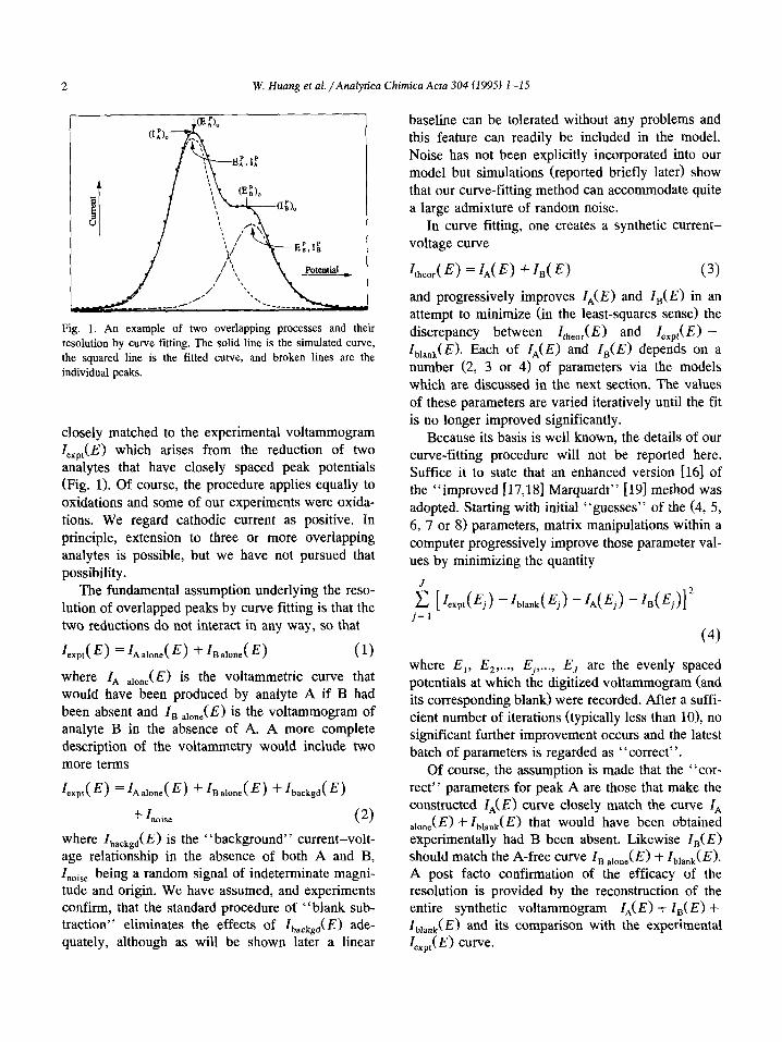
Fig. 1. An example of two overlapping processes and their

resolution by curve fitting. The solid line is the simulated curve,

the squared line is the fitted curve, and broken lines are the

individual peaks.

closely matched to the experimental voltammogram Z,,,,(E) which arises from the reduction of two analytes that have closely spaced peak potentials (Fig. 1). Of course, the procedure applies equally to oxidations and some of our experiments were oxida- tions. We regard cathodic current as positive. In principle, extension to three or more overlapping analytes is possible, but we have not pursued that possibility.

The fundamental assumption underlying the reso- lution of overlapped peaks by curve fitting is that the two reductions do not interact in any way, so that

Z,,,,(E) = ZAalone(E) + Znarone(E) (1)

where Z, alone(E) is the voltammetric curve that would have been produced by analyte A if B had been absent and I n =,,,,JE) is the voltammogram of analyte B in the absence of A. A more complete description of the voltammetry would include two more terms

Z,,,,(E) =Z~arone(E) + Zua,one(E) + Zbac&)

+ 'noise (2)

where Z,,,,,,(E) is the “background” current-volt- age relationship in the absence of both A and B, Inoise being a random signal of indeterminate magni- tude and origin. We have assumed, and experiments confirm, that the standard procedure of “blank sub- traction” eliminates the effects of Z,,,,,(E) ade- quately, although as will be shown later a linear

baseline can be tolerated without any problems and this feature can readily be included in the model. Noise has not been explicitly incorporated into our model but simulations (reported briefly later) show that our curve-fitting method can accommodate quite a large admixture of random noise.

In curve fitting, one creates a synthetic current- voltage curve

Zttleor( E) = Z*( J% + ZB( E) (3)

and progressively improves Z,(E) and Z,(E) in an attempt to minimize (in the least-squares sense> the discrepancy between Ztheor(E) and Z,,,,(E) - Iblank( Each of Z,(E) and Z,(E) depends on a number (2, 3 or 4) of parameters via the models which are discussed in the next section. The values of these parameters are varied iteratively until the fit is no longer improved significantly.

Because its basis is well known, the details of our curve-fitting procedure will not be reported here. Suffice it to state that an enhanced version [16] of the “improved [17,18] Marquardt” [19] method was adopted. Starting with initial “guesses” of the (4, 5, 6, 7 or 8) parameters, matrix manipulations within a computer progressively improve those parameter val- ues by minimizing the quantity

i ['exptlEj) -zblank(Ej) -z*(Ej> -zE%(E,)]2

j=l

(4)

where E,, E, ,..., Ej ,..., E, are the evenly spaced potentials at which the digitized voltammogram (and its corresponding blank) were recorded. After a suffi- cient number of iterations (typically less than lo), no significant further improvement occurs and the latest batch of parameters is regarded as “correct”.

Of course, the assumption is made that the “cor- rect” parameters for peak A are those that make the constructed Z,(E) curve closely match the curve IA a,one(E) + Z,,lank(E) that would have been obtained experimentally had B been absent. Likewise Z,(E) should match the A-free curve In a,one(E) + Z,,,,,(E). A post facto confirmation of the efficacy of the resolution is provided by the reconstruction of the entire synthetic voltammogram Z,(E) + Z,(E) + Z,,,,(E) and its c omparison with the experimental Z,,,,(E) curve.

W. Huang et al. /Analytica Chimica Acta 304 (1995) 1-15 3

An early step in the building of a model for a

voltammetric peak is to select a set of parameters. We have eschewed a choice based on chemically

significant parameters (concentrations, standard po- tentials, rate constants) in favour of more voltammet-

rically relevant quantities: the peak coordinates EP

and Zp, the reversibility index A, and the symmetry factor a. The reversibility index is the dimensionless

quantity defined by

A = kOdm (5)

where k” is the standard heterogeneous rate con- stant, D is a mean diffusion coefficient, and At is

the characteristic time interval of the voltammetric

method, such as a pulse time, drop time or reciprocal frequency. Notice that we are treating the electron

number n and the temperature T as known constants. The diffusion coefficient D is not necessarily known;

it does not appear explicitly as a parameter, however, being “buried” in the quantities ZP and A.

One advantage of this choice of parameters is that

it provides easy and appropriate “guessed” values of EP and Zp to initialize the Marquardt optimiza-

tion procedure. Fig. 1 illustrates this. It shows a

voltammogram in which the peaks arising from species A and B are severely overlapped. The values

marked as ( E,Pjo and (ZAP>,, can be used as initial

guesses of El and Ii, with <E$>o and (ZgPjO being employed similarly. When the voltammograms are so badly merged that only a single peak appears, its location may be used to initialize both Ei and EE,

while its height can be the “guessed” value of both Ii and ZSp. The ability to make sensible guesses in

this way is very valuable when automatic instrumen-

tation is being used to implement resolution by curve

fitting. We used the values 1.000 and 0.500, respec-

tively, as initial guesses of A and LY.

3. The model

In its most general formulation, the model that we

used for a voltammetric peak is

f{ E(T) - f( E/U}

Z(E) =IP f{o) -f{l/fl} (6)

The peak current Zp appears as a multiplier, while

the peak potential EP is present within the E param-

eter

E=~~~{(~F/RT)(E~-E))

The (T term is a known constant

(7)

u = exp{ ( nF/RT) ( AE/Z)} (8)

and incorporates the dependence of the voltammetric

signal on AE, which equals the pulse height in pulse

voltammetries, or has an equivalent significance for

other techniques. The two kinetic parameters, LY and A, are incorporated into the definition, namely

(9)

of the f(x) function. L is used as an abbreviation for

A’ + A2 + A I,,’ 0

L= A3 + A2 + A -t 1

( 10)

which may be written equivalently as [(A4 -

Al/CA” - l>l”” but we avoid this succinct repre- sentation because it becomes indeterminate when A= 1.

This complicated model is employed in its en- tirety for quasireversible voltammetric peaks. It may also be employed for voltammograms from species

whose degree of reversibility is unknown. Irreversible voltammograms are characterized by

a small value of A. Consequently L then becomes

equal to Aila and is greatly exceeded by x. In these

circumstances, the definition of the f{x} function

simplifies to

f{ x) = x a exp{ x2 a/rr}erfc{ x U/&} (irreversible)

(11)

so that the dependence on the A parameter disap-

pears. Conversely, reversibility corresponds to a large

value of A. In that limit, L equals unity and f(x) therefore acquires the form

x”exp{A2(1 +x)~/(?T_x-~~)}

xerfc{A(l +.x)/(&x’~~)}

4 W. Huang et al. /Analytica Chimica Acta 304 (1995) l-15

However, when, as here, its argument is large, the exp{ z2}erfc{r} product becomes equal to l/ Gz, so that

f{x} = X A(1 +x)

(reversible) (12)

Moreover, Eq. 6 then simplifies to

Z(E) “ZP E(l + o)*

(e+u)@+1) (reversible) (13)

Thus the model for a reversible peak has only two unknown parameters: the peak current ZP and (via E) the peak potential EP.

In constructing our model, we leaned heavily on the theory of pseudo-derivative normal pulse po- larography [20-231. For that technique, Eq. 13 is known to be exact under reversible conditions. Simi- larly the combination of Eqs. 6 and 11, though incorporating small errors otherwise, is obeyed by irreversible pseudo-derivative normal pulse polarog- raphy when AE is sufficiently small. Eq. 9 itself is empirical; it was selected because it reduces appro- priately to Eq. 11 or 12 for extreme values of the reversibility index A, is consistent with theory for the small amplitude case available with some tech- niques 1241 and because it provides an excellent numerical match to simulated quasireversible pseudo-derivative normal pulse polarograms.

Despite its origins in the pseudo-derivative tech- nique, there are good reasons for the belief that the model should also fit many other electroanalytical methods that generate peak-shaped current-voltage curves [25]. In the subsequent sections of this paper, we shall describe successful applications to voltam- mograms (at glassy carbon and stationary mercury electrodes) and polarograms (at dropping mercury electrodes) generated by three electroanalytical tech- niques: differential pulse, pseudo-derivative normal pulse, and square wave. The approach should also be applicable to semidifferentiated linear-potential- sweep voltammetry, a.c. polarography and other techniques.

3.1. Background current

If a baseline current I, is a linear function of potential E, which is a good approximation over a narrow potential range, then

Z,=a+bE (14

3

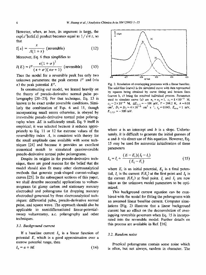
Fig. 2. Resolution of overlapping processes with a linear baseline.

The solid line (curve) is the simulated curve with data represented

by squares being obtained by curve fitting and broken lines

(curves b, c) being the resolved individual process. Parameters

used to simulate curve (a> are trt = n2 = 1, cr = 1 X10e4 M,

c2 = 2X 1O-4 M, AE,,, = - 100 mV, T = 298.2 K, A = 0.01

cm*, D, = D, = 4 X 10W6 cm* s-r, tp = 0.045, Ester, = 1 mV,

E l/2.1 = - 500 mV.

where a is an intercept and b is a slope. Unfortu- nately, it is difficult to generate the initial guesses of a and b via direct use of this equation. However, Eq. 15 may be used for automatic initialization of these parameters

z =z, + (E-Ei)(zt-zi) b I

tEf- Ei) (15)

where E, is an initial potential, E, is a final poten- tial, Zi is the current Z(Ei) at the first point and Zr is the current ICE,) at final point. Zi and Zr are now taken as the unknown model parameters to be opti- mized.

This background current equation can be com- bined with the model for fitting the polarograms with an assumed linear baseline current. Computer simu- lations (Fig. 2) illustrate that a linear background current has no effect on the deconvolution of over- lapping reversible processes when Eq. 15 is incorpo- rated into the reversible model. Further details on this process are available in Ref. [16].

3.2. Random noise

Practical polarograms contain some noise which is often, but not always, random in character. The

W. Huang et al. /Analytica Chimica Acta 301 (1995) I-I.5 5

background current considered above, would be de-

scribed as systematic or non-random noise. To evaluate the influence of random noise in

applying curve fitting methods, the noise may be

added to the Faradaic current response point by point so as to mimic the practical situation

‘t = ‘Far,j + ‘noise j (16)

Random noise is, of course, not correlated with the values of the Faradaic current nor the values of the

corresponding abscissae (i.e., the potential) at each

point. A simulated noisy polarogram (Fig. 3) is

therefore produced by adding Gaussian noise to a

noise-free polarogram [16,27]. In Fig. 3, the value of the signal-to-noise ratio is 10 and the Faradaic re-

sponse clearly is visible. However, if the amplitude of the Faradaic signal is less than or equal to the

noise, i.e., S/N < 1, the Faradaic signal is masked

by the noise. Data in Table 1 demonstrate that

random noise has no marked effect on resolving the

signals of individual components from overlapping processes with S/N = 20 and 10 by the curve fitting

procedure, although a S/N ratio of 5 has a notice- able effect.

3.3. Chemical systems used

dH,

L4;x=o IB ; X=S

Our first examples of overlapping processes de-

rive from binuclear copper complexes having struc- ture I where X = S or 0. The two binuclear com-

plexes differ only in the nature of the endogenous

bridging atom, and may be represented as L(S)Cu,(pz) and L(O)Cu,(pz), where pz symbolises the pyrazolate bridge and L represents the remaining part of the ligand system. A sequence of one-electron charge-transfer processes have been reported for each

compound [26]. However, a major problem in study- ing these binuclear complexes was that strongly overlapping responses made it difficult (or impossi- ble) to determine the required electrochemical pa- rameters accurately. This paper shows how the

curve-fitting method may be successfully applied to

solve this problem. The second class of overlapping processes studied

here derives from mixtures of It-&I) + Cd(B) and Tl(1) i- Pb(I1). Both In(II1) and Cd(B) are reversibly

reduced in aqueous hydrochloric acid at mercury

electrodes according to the processes

In(II1) + 3ee+ In(Hg) (16)

Cd(B) + 2e-+ Cd(Hg) (17)

The In(III), Cd(B) system is regarded as a classical

overlapping response problem in polarography [2,3,11,12] with the reversible half-wave potentials

separated by about 40 mV in 1.0 M HCl. The

reductions of Pb(I1) and Tl(1) at mercury electrodes to their amalgams also are reversible and occur as in

Eqs. 18 and 19, respectively

Pb(II) + Ze--+ Pb(Hg) (18)

Tl( I) + e- + Tl( Hg) (19)

This problem also represents a well-known example of two species giving rise to severely overlapping polarographic signals [3,27-291. For example, their

peak potentials in differential pulse polarography are separated by about 60 mV in 1.0 M ZnSO, acidified

to pH 2 with H,SO, [27].

The example represented by Eqs. 16 and 17 corre- sponds to a case in which a three-electron reversible process overlaps with a reversible two-electron

charge-transfer process. In contrast, the lead(H) and

thallium(I) system involves a reversible two-electron process overlapping with a reversible one-electron

charge-transfer process and the binuclear copper complexes provide reversible one-electron overlap- ping responses. Reversible one-electron processes are considerably broader than two or three-electron

charge-transfer steps so the above examples repre- sent a severe test of overlapping responses con-

structed from different combinations of shapes. The third and final category of reactions consid-

ered concerns the irreversible reduction of chromium and the quasireversible reduction of zinc ions at mercury electrodes. These two species exhibit the

W. Huang et al./Analytica Chimica Acta 304 (1995) 1-15 6

I I -0.7 -016 -0.5 ok -

El Volt

Fig. 3. An example of overlapping processes in the presence of

noise where curve c represents the observed response calculated

as the sum of the noise free response (curve a) and the random

noise (curve b). S/N = 10, other parameters are as for Fig. 2.

following overall reactions at a mercury electrode [30]:

Cr(III) + e-+ Cr(I1) (20)

Zn(I1) + 2e-+ Zn(Hg) (21)

Table 1

Therefore, the Cr(III)/Cr(II) reaction is one-electron charge transfer process with the product of reaction, C&I), being soluble in aqueous solution. In contrast, the Zn(II>/Zn(Hg) reduction involves a two-electron charge transfer and the product, elemental zinc, forms an amalgam with the mercury electrode. A mixture of C&II) and Zn(I1) therefore provides a good ex- ample of overlapping irreversible, solute-forming, and quasireversible, amalgam-forming, processes. The individual processes for reduction of chromium and zinc ions have been the subjects of extensive studies [24,30-321. However, the overlapping re- sponses of these two species under conditions of differential pulse polarography and pseudo-deriva- tive normal pulse polarography have not been re- ported, although data on overlapping DC polaro- graphic waves for reduction of chromium and zinc ions are available [12].

The Cr(II1) and Zn(I1) system, as well as provid- ing an opportunity to assess the general model for resolution of overlapping kinetically controlled pro- cesses, also provides a thorough test of our model.

4. Experimental

Chemicals Unless otherwise specified, all chemicals used

were of analytical grade purity. The binuclear com- plexes L(S)Cu,(pz) and L(O)Cu,(pz) were prepared as described in Ref. [26] and dried under vacuum for 8 h.

Effect of random noise on the resolution of overlapping reversible processes a

S/N Peak Expected Calculated Error b

IP EP

:;A)

EP RE(IP) AE(EP) ( I.LA) (mV) (mV) (D/o) (mV)

20 1 1.046 - 490 1.091 - 488.7 4.3 1.3

2 2.092 - 590 2.155 -589.8 3.0 0.2 10 1 1.046 - 490 1.143 - 487.4 9.3 2.6

2 2.092 -590 2.227 - 589.6 6.5 0.4 5 1 1.046 - 490 1.261 - 484.5 20.1 5.5

2 2.092 -590 2.376 - 589.7 13.6 0.3

an~=n~=1,c~=1X10~4M,c~=2~10~4M,E~,21=500mV,AE~,,=

cm2 s-r, tp = 0.04 s, Eslep = 1 mV. 100 mV, T = 298.2 K, A = 0.01 cm’, D, = D, = 4 X 10m6

b RE(I,? = I&, , j/I&, , - 1 and AE(E,r) = .Qj - E&,,,.

W. Huang et al. /Analytica Chimica Acta 304 (1995) I-15 7

To prepare the required metal ion solutions in

aqueous media, appropriate volumes of standard so- lutions of Cd(NO,),, In(NO,),, Pb(NO,),, TlNO,,

Cr(NO,), and Zn(NO,), supplied by BDH, were added to the electrolyte.

For studies with the binuclear complexes, HPLC- grade dichloromethane and electrochemical grade te-

trabutylammonium tetrafluoroborate electrolyte pur- chased from Southwestern Analytical Chemicals

(Austin, TX), were used, after drying under vacuum for at least 8 h.

Instrumentation and procedures

All solutions for voltammetric studies were de-

oxygenated for 5 min with high purity nitrogen prior

to experiments. Data are reported for a temperature

of 25 f lo C. Polarographic data for the study of the overlap-

ping indium and cadmium processes were obtained

with a Metrohm Model 646 Voltammetric Analysis

Processor and a Metrohm Model 647 electrode as- sembly. The Metrohm Model 647 contains a multi-

mode mercury working electrode [which may be used as a dropping mercury electrode (DME), a static mercury drop electrode (SMDE) or a hanging

mercury drop electrode (HMDE)], an aqueous

Ag/AgCl (saturated KC0 reference electrode and a glassy carbon auxiliary electrode.

Polarograms for the overlapping lead and thallium

processes were obtained with a BASlOO electro-

chemical analyzer used in conjunction with a PAR Model 303 static mercury drop electrode system

(SMDE or HMDE modes), a Ag/AgCl (saturated KCl) reference electrode and a platinum auxiliary

electrode. Voltammetric measurements on the binuclear cop-

per complexes were performed with the BAS-100

electrochemical analyzer at platinum disk (Pt), gold disk (Au) and glassy carbon disk (GC) electrodes. The solid working electrodes were polished fre- quently with an aqueous alumina slurry, followed by

rinsing with water and then with solvent (CH,CI,). This cleaning treatment was required to obtain repro- ducible results. The auxiliary electrode was a plat- inum wire and the reference electrode was Ag/AgCl (CH,Cl,; saturated LiCl). Potentials in dichloro- methane are referenced to the potential of the Fc/ Fc’ process [Fc = ferrocene, ($-C,H&Fe] via

measurement of the reversible potential versus Ag/AgCl for oxidation of a 5 X 10S4 M solution of ferrocene in dichloromethane.

The experimental data were transferred from the Metrohm 646 VA Processor or the BAS-100 Ana-

lyzer to a SPHERE microcomputer and then either to a mainframe DEC-20 computer or to an IBM per-

sonal computer for processing. Unless otherwise stated, the experimental condi-

tions used for voltammetric measurements with the BAS-100 equipment were:

(i)

(ii)

Normal and differential pulse voltammetry

(polarography): drop time or duration between

pulses 1 s; pulse time 0.06 s, current sampling time 0.02 s; pulse amplitude - 50 mV; scan rate

- 2 mV s -’ ; potential step - 2 mV. Square-wave voltammetry (polarography): drop

time 1 s; square-wave amplitude 25 mV:

square-wave frequency 12 Hz: potential step - 2

mV. The measurement parameters used with the Metrohm

equipment, except where stated, were as follows: (i) Normal and differential pulse voltammetry

(polarography): drop time or duration between pulses 0.6 s; pulse amplitude -50 mV; pulse

time 0.04 s, current sampling time 0.02 s; scan rate - 2 mV s _ ’ .

(i> Square-wave voltammetry (polarography): drop

time 0.6 s; square-wave amplitude 25 mV; scan rate -2.5 mV s-‘.

For the studies on the binuclear copper complexes

in dichloromethane, the concentrations of

L(S)Cu,(pz), L(O)Cu,(pz) and ferrocene were all 5 X 10T4 M. the potential step was + 4 mV, the

duration between pulses was 1 s, the potential range examined was from 200 to 1200 mV vs. Ag/AgCl, the scan rate was 4 mV s _I. and other parameters

are as for the above mentioned experiments with the BAS instrument.

5. Results and discussion

Oxidation of hinuclear copper complexes

For the binuclear, L(X)Cu,(pz), complexes the processes studied [26] were the oxidation steps:

L(X)C&(pz) + [L(X)Cu?(pz)] + + em (22)

[LWWPz)l + 4 [L(X)Cuz(pz)]” + e- (23)

8 W. Huang et al. /Analytica Chimica Acta 304 (199.5) 1-15

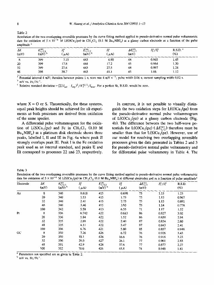
Table 2

Resolution of the two overlapping reversible processes by the curve fitting method applied to pseudo-derivative normal pulse voltammetric

data for oxidation of 5 X 10e4 M L(O)Cu,(pz) in CH,Cl, (0.1 M Bu,NBF,) at a glassy carbon electrode as a function of the pulse

amplitude a

E’“’

l/2,1 If E’W

l/V 14 AE;‘;; Q/If R.S.D. ’

(mV) b ( PA) (ml9 b ( jd CmV) (o/o)

8 399 7.15 443 6.90 44 0.965 1.45

20 399 17.8 444 17.2 45 0.964 1.30

32 399 27.6 443 27.5 44 0.997 1.24

48 398 38.7 443 41.1 45 1.06 1.12

a Potential interval 4 mV; duration between pulses 1 s; scan rate 4 mV s-‘; pulse width 0.06 s; current sampling width 0.02 s.

b mV vs. Fc/Fc+.

’ Relative standard deviation = [x(1,,, - 1,,,)2/N]‘/2/I,,,. For a perfect fit, R.S.D. would be zero.

where X = 0 or S. Theoretically, for these systems, equal peak heights should be achieved for all experi- ments as both processes are derived from oxidation of the same species.

A differential pulse voltammogram for the oxida- tion of L(S)Cu,(pz) and Fc in CH,Cl, (0.10 M Bu,NBF,) at a platinum disk electrode shows three peaks, labelled I, II and III in Fig. 4a where peak II strongly overlaps peak III. Peak I is the Fc oxidation peak used as an internal standard, and peaks II and III correspond to processes 22 and 23, respectively.

In contrast, it is not possible to visually distin- guish the two oxidation steps for L(O)Cu,(pz) from the pseudo-derivative normal pulse voltammogram of L(O)Cu,(pz) at a glassy carbon electrode (Fig. 4b). The difference between the two half-wave po- tentials for L(O)Cu,(pz) ( AEIe’,) therefore must be smaller than that for L(S)Cu, pz). However, use of i our model for resolving two overlapping reversible processes gives the data presented in Tables 2 and 3 for pseudo-derivative normal pulse voltammetry and for differential pulse voltammetry in Table 4. The

Table 3

Resolution of the two overlapping reversible processes by the curve fitting method applied to pseudo-derivative normal pulse vohammetric

data for oxidation of 5 X 10e4 M LWCu,(pz) in CH,Cl, (0.1 M Bu,NBF,) at different electrodes and as a function of pulse amplitude”

Electrode

pm”v,

ETeV 1/U If Erev w,2 I$ AEi”;z &T/If R.S.D.

(mV) b ( pAI (mV) b ( PA) (mV) (%I

Au 8 340 0.618 415 0.698 75 1.13 1.23

20 340 1.53 415 1.73 75 1.13 0.967

32 340 2.41 415 2.73 75 1.13 0.891

48 340 3.46 415 3.93 75 1.14 0.778

100 342 5.58 413 6.55 71 1.17 1.52

8 336 0.742 422 0.613 86 0.827 3.02

20 336 1.84 422 1.52 86 0.830 2.94

32 335 2.88 422 2.40 87 0.834 2.80

48 335 4.11 422 3.47 87 0.843 2.41

100 336 6.76 421 5.80 85 0.857 0.948 GC 8 350 7.26 426 6.72 76 0.926 3.43

20 350 18.1 426 16.6 76 0.916 3.23

32 350 29.0 427 26.1 77 0.901 2.83

48 351 42.9 428 37.6 77 0.877 2.27

100 352 70.0 426 65.8 74 0.940 1.81

a Parameters not specified are as given in Table 2. b mV vs. Fc/Fc+.

W. Huang et al./Analytica Chimica Actu 304 11095) 1-15 0

II III (a)

f-i

O-9

II+III

T I /\ m,i-_ 0

ENolt vs. FclFc+ 0.5

Fig. 4. Pulse voltammograms for oxidation of 5 X 10M4 M each of

ferrocene (process I) and L(X)Cu,(pzl (processes II and III) in

dichloromethane (0.10 M Bu,NBF,l. (a) Differential pulse

voltammograms for oxidation of L@)Cu,(pz) at a platinum elec-

trode. AE = - 10 mV. (bl Pseudo-derivative normal pulse

voltammogram for oxidation of L(0)Cuz(pz) at a glassy carbon

electrode. AE = - 20 mV.

E ;‘;; values in Tables 2 to 4 are calculated from the

relationship E;“;; = E, - AE/2.

Table 2 shows that, as theoretically expected, the

half-wave potentials for the oxidation of L(O)Cu,(pz)

at a glassy carbon electrode are independent of pulse amplitude. The two peak currents, 11p and Z2p, in- crease as the pulse amplitude increase, but their ratio

remains close to unity, again as theoretically ex- pected. Furthermore, the relative standard deviation, a criterion of the goodness of fit, is very small.

Results close to those theoretically expected also are

found for L(S)Cu,(pz) (Tables 3 and 4) and confirm

that the curve-fitting method may be usefully applied for the resolution of overlapping reversible pro-

cesses, using either pseudo-derivative or differential pulse voltammetry at solid electrodes.

In the case of L(S)Cu,(pz), a slight dependence

of the calculated half-wave potentials on electrode material is evident under conditions of pseudo-de- rivative normal pulse voltammetry. However, this is

less evident with the differential pulse voltammetric

method. The variation of calculated EyL with the pseudo-derivative normal pulse voltammetric method

is mainly attributable to the presence of a non linear

baseline, which is electrode dependent and therefore

not accounted for by the model, which accommo-

dates a linear baseline only. In the differential pulse method, a relatively flat baseline is observed and AE;;‘2 is calculated to be 75 mV at a gold electrode,

81 mV at a platinum electrode and 79 mV at a glassy carbon electrode. These AEf;V? values are consistent with the estimated literature value of 80-90 mV

La. The data for oxidation of L(X)Cu,(pz) show that

curve fitting methods based on deconvolution of

reversible overlapping processes are highly reliable by either the pseudo-derivative normal pulse or dif-

ferential pulse voltammetric techniques provided the baseline is linear, as required by the model. In the

case of the oxidation of L(X)Cu,(pz) the non-linear baseline causes some departure from ideality in the

deconvolution polarogram.

InOII) + Cd(U) system

Fig. 5 shows that the fitting of an experimental

differential pulse polarogram obtained for a mixture

Table 4

Resolution of hvo overlapping reversible processes by the curve fitting method applied to differential pulse voltammetric data for oxidation

of 5 X 10m4 M L(S)Cu,(pz) in CH,Cl, (0.1 M Bu,NBF,) at different electrodes and as a function of pulse amplitude ’

Electrode

::v,

Ere’ l/2,1 IP EreV

(mV) b l/2.2 If AE;;‘, Q/V R.S.D.

( PA) (rnv) b ( PA) (rnv) (%r)

AU 10 336 0.846 411 0.892 75 1.05 1.Y9

50 336 3.92 410 3.87 74 0.986 OS23

Pt 10 335 0.744 416 0.745 81 1 .oo 1.46

50 338 3.65 419 3.45 81 0.040 0.877

GC 10 331 8.77 410 8.73 79 0.995 1.29

50 337 38.5 415 33.9 78 0.881 0.767

a Parameters not specified are as given in Table 2 or the Experimental section. b mV vs. Fc,‘Fc+

10 W. Hung et al. /Analytica Chimica Acta 304 (1995) l-15

I I I I -0.55 -0.70

I J - . - . -0.75

EN vs. AgIAgCI

Fig. 5. Comparison of experimental (. .) and calculated (solid

line) differential pulse polarograms with AE = - 10 mV for re-

duction of a mixture of 1.74 X lo-’ M In(III) and 3.56 X 10m5 M

Cd(B) in 1.0 M HCl. The current axis has been normalized by

division by the maximum current I,,,,,

of In(II1) and Cd(U) in 1.0 M HCl at a small pulse amplitude ( AE = - 10 mV) is excellent since the residual is very small. However, the fit is worse in differential pulse polarography when a large pulse amplitude is used because a significant d.c. compo- nent is introduced into the experiment which is not eliminated in any subtraction process [33]. Thus, Fig. 6a illustrates that fits to the experimental data with a large pulse amplitude ( AE = 100 mV) are not as good as for the small amplitude curve (Fig. 5). The discrepancies caused by the d.c. term in Fig. 6a is most noticeable around the peak and at the negative potential region of the polarogram. If it is assumed that a linear baseline problem is present then the problem of the d.c. offset can be minimised (Fig. 6b). Table 5 presents data obtained by the differen- tial pulse method at a DME and HMDE and square wave polarography at the DME. Table 6 lists results obtained by the different methods as a function of the concentration ratio of In(II1) to Cd(H).

Table 5

Data obtained for resolution of overlapping In(III1 and Cd(B) processes in 1 M HCl (concentrations: In(III), 1.74 X 10m5 M; Cd(B),

3.56 x lo-’ M)

(Al differential pulse polarography at the DME and differential pulse voltammetry at the HMDE a

Electrode Species Expected b

IP

( ~4)

EP

CmV)

Calculated ’

DME -10 In011)

Cd(B)

-100 In(III)

Cd(B)

HMDE - 10 In(III)

Cd(B)

- 100 In(II1)

Cd(B)

(B) Square wave polarography at DME d

0.195 -598 0.1953

0.185 - 638 0.1850

0.704 -598 0.7118

0.976 - 638 0.9410

0.0766 - 598 0.07401

0.0872 - 642 0.09120

0.260 - 598 0.2605

0.398 - 640 0.3769

-598

- 640

-599

- 638

- 599

- 643

- 599

- 642

Species Experimental

EP

(mV1

Calculated

IP

( /LA)

EP

(mV)

5 In(III) 0.0768 -598 0.07760 -591

Cd(B) 0.0825 - 638 0.08251 - 640

25 In(III) 0.352 -598 0.3515 - 597

Cd(B) 0.382 -638 0.3871 -639

a Experimental parameters are: drop time, 1 s; potential step, 2 mV; scan rate, 2 mV s-t ; pulse width, 0.04 s; current sampling width, 0.02

S.

b Values obtained from experimental measurements on single component solutions.

’ Values obtained on mixtures of the two components and use of the model developed in this paper to resolve overlapping voltammetric

processes.

d Parameters not stated are defined in the text.

W. Hung et al. /Anal.ytica Chimica Acta 304 (1095) I-15 II

For the overlapping I&II) + Cd(H) system in 1.0

M HCl, two partially overlapped peaks are observed if AE is 10 mV (see Fig. S), but only one peak appears when AE is 100 mV (Fig. 6). However, as

can be seen from Table 5, excellent recovery of the

expected values is obtained even when AE is as large as 100 mV. The expected values in Table 5 and elsewhere were determined from data obtained from

measurements on single component systems. It

should be noted that for differential pulse polarogra-

phy with the BAS 100 instrument, the potential axis is plotted on the basis of the potential (E,) before the pulse so the peak potential is a function of AE.

However, with the Metrohm instrument, the peak position of individual electroactive species is inde-

pendent of the pulse amplitude as (E, + E,)/2 rather

than E, is used as the basis of the potential axis, Ez

being the potential after the pulse. The concentration ratio also affects the shape of

the overlapping processes. For the I&II) + Cd(II)

system in 1.0 M HCl, when the concentration ratio

of I&II) to Cd(I1) [c(Cd>/c(In>] is less than 1, a single peak is observed and the apparent peak poten- tial is very close to the peak potential of In(III).

When c(Cd)/c(In) is near 2, two peaks are ob-

served, but when c(Cd)/cUn) > 3, a single peak reappears. However, under these conditions the ap-

parent peak potential is close to the peak potential of Cd(II). Despite the peak potential and shape change, data in Table 5 indicate that the curve-fitted results

for resolution of overlapping differential pulse and square wave processes at both the DME and HMDE

Table 6

Effect of concentration ratio on the resolution of overlapping processes for a mixture of In(III) and Cd(U) in 1 M HCI with different

voltammetric techniques and pulse amplitudes a

(A) Differential pulse polarography at the DME and differential pulse voltammetry at the HMDE

Electrode c(Cd)/ c(In) Species Expected Calculated

IP

( /LA) E”,

IP E p

( /LA) (mV)

DME 0.511 In(II1) 0.710 -594

Cd(B) 0.191 - 63h 2.04 In(III) 0.362 -594

Cd(B) 0.370 - 630 10.2 In(III) 0.362 - 594

Cd(II) 1.82 - 63f> HMDE 0.511 In(III) 0.312 -5’):

Cd(B) 0.100 -63(1 2.04 In(III) 0.143 -59x

Cd(B) 0.190 -63X 4.09 In0111 0.143 -598

Cd(H) 0.363 - h38

(B) Square wave polarography at the DME and square wave voltammetry at the HMDE

0.6991

0.1920

0.3574

0.3559

0.3698

1.815

0.3237

0.1012

0.1443

0.1852

0.1498

0.372’

-5Yl

- h32

- 596

-637 _ 545

- h3h

- 5Y3

- 632

-5Y7

- 639

-594

- h37

DME 0.511 In(III) 0.550 - s92 0.5522

Cd(B) 0.165 - 63h 0.1693 2.04 In0111 0.276 - 592 0.2804

Cd(B) 0.316 - 636 0.3082

4.09 In010 0.276 - 592 0.2829

Cd(B) 0.621 - 636 0.6202 HMDE 0.511 In(II1) 0.282 -596 0.2723

Cd(B) 0.0886 - 640 0.09371 2.04 In(III) 0.140 - 596 0.13Y7

Cd(U) 0.190 ~ 640 0.1825 4.09 In010 0.140 - 596 0.1427

Cd(B) 0.361 - 640 0.3731

- 5Y3

- 634

-5Y5

- 637

-5Yl

- 633 -506

- 638

-5Y6

ph4l -504

- 638

a Experimental parameters and definitions of terms are the same as in Table 5 except c(Cd)/c(In): 1.78 X lo- M/3.48 X 10mi

M = 0.51 I, 3.56 X 1O-5 M/1.74 x lo-’ M = 2.04, 7.12 x lo--’ M/1.74 x IO-’ M = 4.09, 1.78 x 10-j M/1.74 x IO-' M = 10.2.

12 W. Huang et al. /Analytica Chimica Acta 304 (1995) l-15

I I I 4

-0.50 -0.55 -0.60 -0.66 -0.70 -0.75

EN vs. AglA$l

I I 1 c -0.50 -0.55 -0.60 -0.65 -0.70 -0.75

Fig. 6. Comparison of experimental (. .) and calculated (solid

line) differential pulse polarograms with AE = - 100 mV for

reduction of a mixture of 1.74 X 10W5 M In(III) and 3.56 X 10m5

M Cd(R) in 1.0 M HCl. The reversible model was used assuming

the absence of a baseline in (a) and with addition of a linear

baseline in (b) for the curve fitting.

for the concentration ratios of c(Cd)/c(In) from 0.5 to 10 are in excellent agreement with the theoreti-

cally expected results. Data in Table 6 also confirm

9 -0.3 -0.4 -0.5

(b)

4 EN vs. Ag/AgCl

Fig. 7. Normal (a) and pseudo-derivative (b) pulse polarograms

for the reduction of a mixture of 1.21 X 10m4 M Pb(I1) and

9.62X 10m4 M Tl(1) in 1.0 M ZnSO,.

that the curve-fitting method for reversible processes

can be applied for different values of AE, different concentration ratios, different techniques and differ- ent forms of mercury electrode.

Pb(II) + TICI) system

It is impossible to visually distinguish two re-

sponses from the normal pulse polarogram (Fig. 7a) for the reduction of the Pb(I1) + Tl(1) system in the supporting electrolyte of 1.0 M ZnSO,. However,

Table 7

Resolution of overlapping processes for a mixture of 1.2 X 1O-4 M PM111 and 9.6 X 10m4 M TI(Il in 1 M ZnSO, using a range of

voltammetric techniques a

Technique AE (mV1 Ion Expected Calculated

IP I* EP

( /LA) ( CLA) (mV)

PDNPP a - 10 Pb(II) 0.189 - 400 0.186 - 400

PDNPP a

PDNPP a

SWP

DPP a

-50

-100

5

- 10

no) 0.404 -458 0.409 - 459

PbtIIl 0.742 -381 0.689 - 380

Tl(I) 1.87 - 437 1.888 - 438 Pb(II) 0.939 - 356 0.918 - 360

n(I) 3.01 -412 3.077 -410 Pb(II) 0.198 - 408 0.187 - 408

n(I) 0.429 - 468 0.440 - 469

Pb(I1) 0.184 -414 0.192 -414

-INI) 0.418 - 474 0.429 - 474

a Experimental parameters are: drop time, 1 s; pulse width, 0.06 s; current sampling time, 0.02 s; scan rate, 2 mV s- ‘. Other experimental

parameters and terms are defined in the text or in previous tables. PDNPP = pseudoderivative normal pulse polarography, SWP = square- wave polarography, DPP = differential pulse polarography.

W. Huang et al./Analytica Chimica Acra 304 (1995) 1-15 13

L -0.7 -0.8 -0.9 -1 .o -1.1 -’

EN vs Ag/AgCl

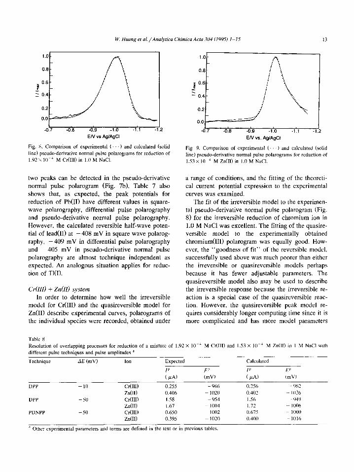
Fig. X. Comparison of experimental (. .) and calculated (solid

line) pseudo-derivative normal pulse polarograms for reduction of

1.92~ lWJ M Cr(III) in 1.0 M NaCl.

two peaks can be detected in the pseudo-derivative normal pulse polarogram (Fig. 7b). Table 7 also

shows that, as expected, the peak potentials for

reduction of Pb(I1) have different values in square- wave polarography, differential pulse polarography

and pseudo-derivative normal pulse polarography. However, the calculated reversible half-wave poten-

tial of lead011 at -408 mV in square wave polarog-

raphy, -409 mV in differential pulse polarography

and -405 mV in pseudo-derivative normal pulse

polarography are almost technique independent as expected. An analogous situation applies for reduc-

tion of Tl(1).

CdIII) + Zn(IIJ system In order to determine how well the irreversible

model for Cr(II1) and the quasireversible model for Zn(I1) describe experimental curves, polarograms of

the individual species were recorded, obtained under

I -0.7 -0.8 -0.9 -1 .o -1.1 -1

EN vs. AglAgCl

Fig. 9. Comparison of experimental (. ) and calculated (solid

line) pseudo-derivative normal pulse polarograms for reduction of

1.53 X 1OY4 M Z&I) in 1.0 M NaCl.

a range of conditions, and the fitting of the theoreti-

cal current-potential expression to the experimental curves was examined.

The fit of the irreversible model to the experimen- tal pseudo-derivative normal pulse polarogram (Fig. 8) for the irreversible reduction of chromium ion in

1.0 M NaCl was excellent. The fitting of the quasire- versible model to the experimentally obtained

chromium(II1) polarogram was equally good. How- ever, the “goodness of fit” of the reversible model,

successfully used above was much poorer than either the irreversible or quasireversible models perhaps

because it has fewer adjustable parameters. The quasireversible model also may be used to describe the irreversible response because the irreversible re-

action is a special case of the quasireversible reac- tion. However, the quasireversible peak model re- quires considerably longer computing time since it is more complicated and has more model parameters

Table X

Resolution of overlapping processes for reduction of a mixture of 1.92 X 10-j M Cr(III) and 1.53 X lo-” M ZnfII) in I M NaC’I with

different pulse techniques and pulse amplitudes a

Technique LIE (mV) Ion Expected Calculated

IQ

( /LA)

EP

tmV1

I” EP

(/LA) (mV1

DPP - 10 CliIII) 0.255 - 966 0.256 - 962

Zn(II) 0.406 - 1020 0.402 -- 11126

DPP - 50 CiiIII) 1.58 - 954 1.56 _ 949 ZntIIl 1.67 - 1004 1.72 - IO06

PDNPP -50 Cr(IIIl 0.650 - 1002 0.675 - 1000 Zn(II1 0.395 - 1020 0.400 - 1016

a Other experimental parameters and terms are defined in the text or in previous tables.

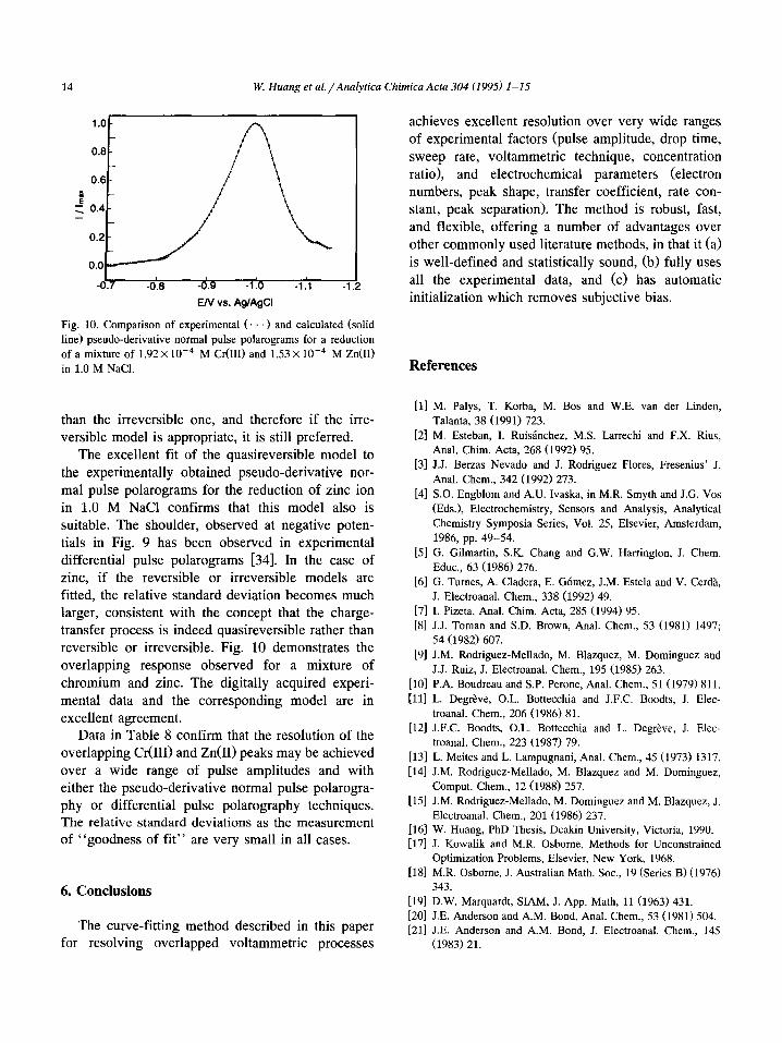
14 W. Huang et al./Analytica Chimica Acta 304 (1995) l-15

-05 -0.8 -0.9 -1.0 -1.1 -1

EN vs. As/AgCl

Fig. 10. Comparison of experimental (’ .) and calculated (solid

line) pseudo-derivative normal pulse polarograms for a reduction

of a mixture of 1.92~ 10m4 M CdlII) and 1.53 X 10m4 M Zn(II)

in 1.0 M NaCl.

than the irreversible one, and therefore if the irre-

versible model is appropriate, it is still preferred. The excellent fit of the quasireversible model to

the experimentally obtained pseudo-derivative nor-

mal pulse polarograms for the reduction of zinc ion in 1.0 M NaCl confirms that this model also is suitable. The shoulder, observed at negative poten-

tials in Fig. 9 has been observed in experimental differential pulse polarograms [34]. In the case of

zinc, if the reversible or irreversible models are fitted, the relative standard deviation becomes much larger, consistent with the concept that the charge- transfer process is indeed quasireversible rather than reversible or irreversible. Fig. 10 demonstrates the

overlapping response observed for a mixture of

chromium and zinc. The digitally acquired experi-

mental data and the corresponding model are in excellent agreement.

Data in Table 8 confirm that the resolution of the

overlapping Cr(II1) and Zn(I1) peaks may be achieved over a wide range of pulse amplitudes and with

either the pseudo-derivative normal pulse polarogra- phy or differential pulse polarography techniques. The relative standard deviations as the measurement of “goodness of fit” are very small in all cases.

6. Conclusions

The curve-fitting method described in this paper for resolving overlapped voltammetric processes

achieves excellent resolution over very wide ranges of experimental factors (pulse amplitude, drop time,

sweep rate, voltammetric technique, concentration ratio), and electrochemical parameters (electron numbers, peak shape, transfer coefficient, rate con-

stant, peak separation). The method is robust, fast,

and flexible, offering a number of advantages over

other commonly used literature methods, in that it (a) is well-defined and statistically sound, (b) fully uses

all the experimental data, and (c) has automatic initialization which removes subjective bias.

References

[l] M. Palys, T. Korba, M. Bos and W.E. van der Linden,

Talanta, 38 (1991) 723.

[2] M. Esteban, I. Ruisanchez, MS. Larrechi and F.X. Rius,

Anal. Chim. Acta, 268 (1992) 95.

[3] J.J. Berzas Nevado and J. Rodriguez Flores, Fresenius’ J.

Anal. Chem., 342 (1992) 273.

[4] S.O. Engblom and A.U. Ivaska, in M.R. Smyth and J.G. Vos

(Eds.), Electrochemistry, Sensors and Analysis, Analytical

Chemistry Symposia Series, Vol. 25, Elsevier, Amsterdam,

1986, pp. 49-54.

[5] G. Gilmartin, S.K. Chang and G.W. Harrington, J. Chem.

Educ., 63 (1986) 276.

[6] G. Tumes, A. Cladera, E. Gbmez, J.M. Estela and V. Cerda,

J. Electroanal. Chem., 338 (1992) 49.

[7] I. Pizeta, Anal. Chim. Acta, 285 (1994) 95.

[8] J.J. Toman and S.D. Brown, Anal. Chem., 53 (1981) 1497;

54 (1982) 607.

[9] J.M. Rodriguez-Mellado, M. Blazquez, M. Dominguez and

J.J. Ruiz, J. Electroanal. Chem., 195 (1985) 263.

[lo] P.A. Boudreau and S.P. Perone, Anal. Chem., 51 (1979) 811.

[ll] L. Degrtve, O.L. Bottecchia and J.F.C. Boodts, J. Elec-

troanal. Chem., 206 (1986) 81.

[12] J.F.C. Boodts, O.L. Bottecchia and L. Degreve, J. Elec-

troanal. Chem., 223 (1987) 79.

[13] L. Meites and L. Lampugnani, Anal. Chem., 45 (1973) 1317.

[14] J.M. Rodriguez-Mellado, M. Blazquez and M. Dominguez,

Comput. Chem., 12 (1988) 257.

[15] J.M. Rodriguez-Mellado, M. Dominguez and M. Blazquez, J.

Electroanal. Chem., 201 (1986) 237.

1161 W. Huang, PhD Thesis, Deakin University, Victoria, 1990. [17] J. Kowalik and M.R. Osborne, Methods for Unconstrained

Optimization Problems, Elsevier, New York, 1968.

[181 M.R. Osborne, J. Australian Math. Sot., 19 (Series B) (1976)

343.

[191 D.W. Marquardt, SIAM, J. App. Math, 11 (1963) 431.

[20] J.E. Anderson and A.M. Bond, Anal. Chem., 53 (1981) 504.

[21] J.E. Anderson and A.M. Bond, J. Electroanal. Chem., 145

(1983) 21.

W. Huang et al. /Analytica Chimica Acta 304 (1995) I-15 15

[22] M. Lovric, J.J. O’Dea and J. Osteryoung, Anal Chem., 55

( 1983) 704.

[23] N. Papadopoulos, C. Hasiotis, G. Kokkinidis and G. Papanas-

tasiou, Electroanalysis, 5 (1993) 99.

[24] M.-H. Kim, V.P. Smith and T-K. Hong, J. Electrochem. Sot.

140 (1993) 712; and references cited therein.

[25] J. Spanier and K.B. Oldham, An Atlas of Functions, Hemi-

sphere, Washington, DC, 1987, pp. 392-393.

[26] A.M. Bond, M. Haga, IS. Greece, R. Robson and J.C.

Wilson, Inorg. Chem., 28 (1989) 559.

[27] A.M. Bond and B.S. Grabaric, Anal. Chem., 48 (1976) 1624.

[28] G.E. Batley and T.M. Florence, J. Electroanal. Chem., 55

(1974) 23.

[29] L. Meites, in Polarographic Techniques, 2nd edn., Inter-

science, New York, 1965, pp. 623-670.

[30] W.S. Go, J.J. O’Dea and J. Osteryoung, J. Electroanal.

Chem., 255 (1988) 21.

[31] R. Tammamushi, in Kinetic Parameters of Electrode Rcac-

tions of Metallic Compounds, Butterworths, London, 1975.

[32] W.S. Go and J. Osteryoung, J. Electroanal. Chem.. 233

(1987) 275.

[33] A.M. Bond, Modern Polarographic Methods in Analytical

Chemistry, Marcel Dekker, New York, 1980.

[34] P. Mericam, M. Astruc and Y. Andrieu. J. Electroanal.

Chem., 169 (1984) 207.