curriculum template for ib hl-2 - squarespacemath+hl.pdf · statistics essential questions ......
TRANSCRIPT

Kennebunk High School
Course Outlines
Name of the course:
International Baccalaureate Math HL
Course description:
IB MATH HIGHER LEVEL – HIGH HONORS – 2 Credits over 2 years - STEM IB Math HL I is taken junior year. IB Math HL II is taken senior year. This course caters for students with a good background in mathematics who are competent in a range of analytical and technical skills. The majority of these students will be expecting to include mathematics as a major component of their university studies, either as a subject in its own right or within courses such as physics, engineering and technology. Others may take this subject because they have a strong interest in mathematics and enjoy meeting its challenges and engaging with its problems. In their Senior year students will sit for the IB exam in May and will complete an Exploration. Prerequisite: Successful completion of Advanced Math and Advanced Placement Statistics
Essential Questions:
• When and why should we estimate? • Is there a pattern? • How does what we measure influence how we measure? • How does how we measure influence what we measure or don’t
measure? • What do good problem solvers do especially when they get
stuck? • How precise should this solution be? • What are the limits of this mathematical model and of
mathematical modeling in general?
Kennebunk High School

Kennebunk High School
Prior LearningTopics:

Kennebunk High School

Kennebunk High School
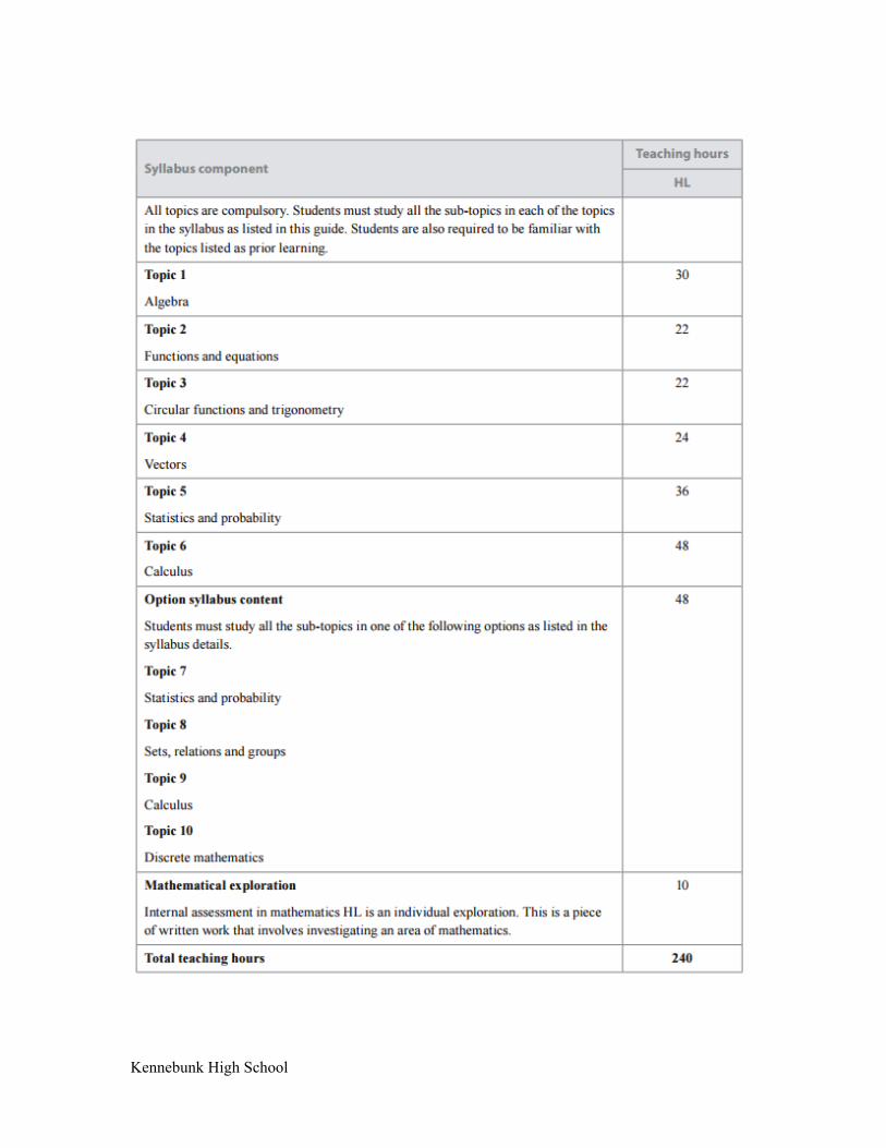
Topics:

Kennebunk High School
Kennebunk High School

Kennebunk High School

Kennebunk High School

Kennebunk High School

Kennebunk High School

Kennebunk High School

Kennebunk High School

Kennebunk High School

Kennebunk High School
Assessment:
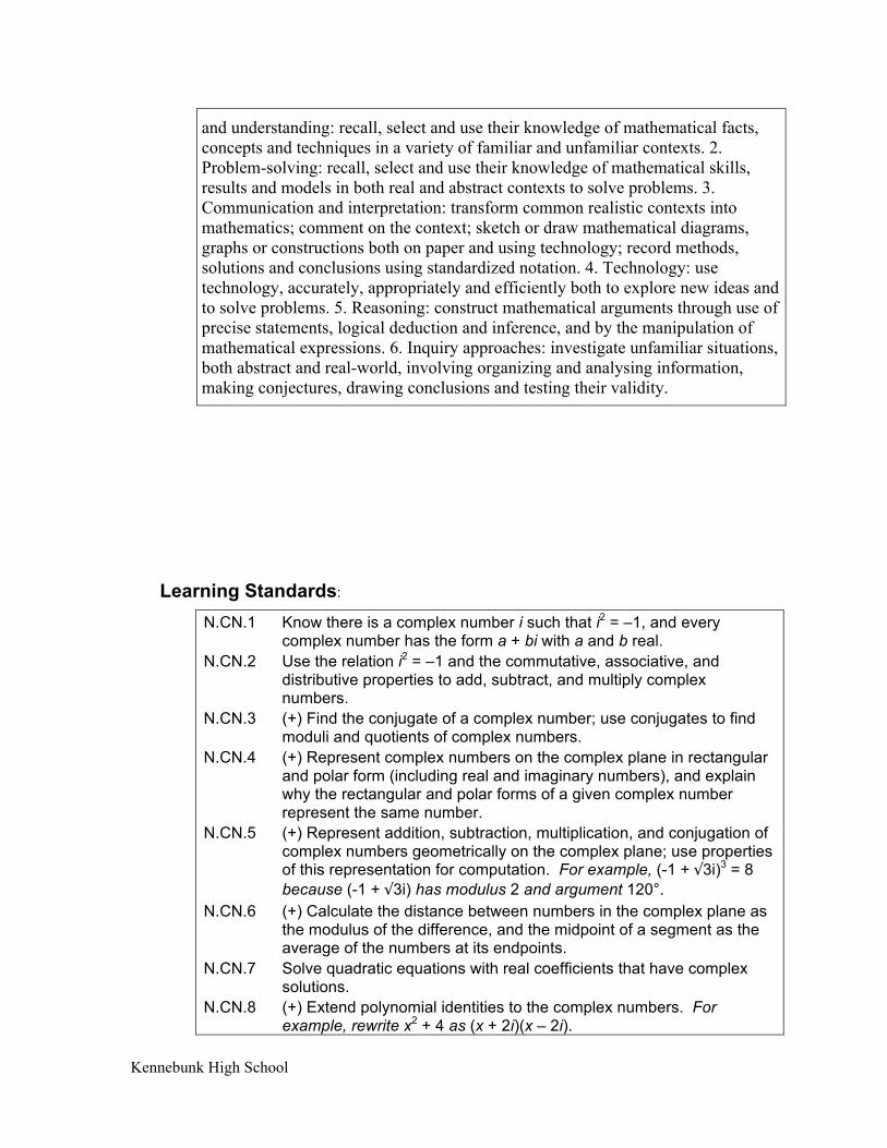
Problem-solving is central to learning mathematics and involves the acquisition of mathematical skills and concepts in a wide range of situations, including non-routine, open-ended and real-world problems. Having followed a DP mathematics HL course, students will be expected to demonstrate the following. 1. Knowledge
Kennebunk High School
and understanding: recall, select and use their knowledge of mathematical facts, concepts and techniques in a variety of familiar and unfamiliar contexts. 2. Problem-solving: recall, select and use their knowledge of mathematical skills, results and models in both real and abstract contexts to solve problems. 3. Communication and interpretation: transform common realistic contexts into mathematics; comment on the context; sketch or draw mathematical diagrams, graphs or constructions both on paper and using technology; record methods, solutions and conclusions using standardized notation. 4. Technology: use technology, accurately, appropriately and efficiently both to explore new ideas and to solve problems. 5. Reasoning: construct mathematical arguments through use of precise statements, logical deduction and inference, and by the manipulation of mathematical expressions. 6. Inquiry approaches: investigate unfamiliar situations, both abstract and real-world, involving organizing and analysing information, making conjectures, drawing conclusions and testing their validity.
Learning Standards: N.CN.1 Know there is a complex number i such that i2 = –1, and every
complex number has the form a + bi with a and b real. N.CN.2 Use the relation i2 = –1 and the commutative, associative, and
distributive properties to add, subtract, and multiply complex numbers.
N.CN.3 (+) Find the conjugate of a complex number; use conjugates to find moduli and quotients of complex numbers.
N.CN.4 (+) Represent complex numbers on the complex plane in rectangular and polar form (including real and imaginary numbers), and explain why the rectangular and polar forms of a given complex number represent the same number.
N.CN.5 (+) Represent addition, subtraction, multiplication, and conjugation of complex numbers geometrically on the complex plane; use properties of this representation for computation. For example, (-1 + √3i)3 = 8 because (-1 + √3i) has modulus 2 and argument 120°.
N.CN.6 (+) Calculate the distance between numbers in the complex plane as the modulus of the difference, and the midpoint of a segment as the average of the numbers at its endpoints.
N.CN.7 Solve quadratic equations with real coefficients that have complex solutions.
N.CN.8 (+) Extend polynomial identities to the complex numbers. For example, rewrite x2 + 4 as (x + 2i)(x – 2i).

Kennebunk High School
N.CN.9 (+) Know the Fundamental Theorem of Algebra; show that it is true for quadratic polynomials.
N.VM.1 (+) Recognize vector quantities as having both magnitude and
direction. Represent vector quantities by directed line segments, and use appropriate symbols for vectors and their magnitudes (e.g., v, |v|, ||v||, v).
N.VM.2 (+) Find the components of a vector by subtracting the coordinates of an initial point from the coordinates of a terminal point.
N.VM.3 (+) Solve problems involving velocity and other quantities that can be represented by vectors.
N.VM.4 (+) Add and subtract vectors. a. Add vectors end-to-end, component-wise, and by the
parallelogram rule. Understand that the magnitude of a sum of two vectors is typically not the sum of the magnitudes.
b. Given two vectors in magnitude and direction form, determine the magnitude and direction of their sum.
c. Understand vector subtraction v – w as v + (–w), where –w is the additive inverse of w, with the same magnitude as w and pointing in the opposite direction. Represent vector subtraction graphically by connecting the tips in the appropriate order, and perform vector subtraction component-wise.
N.VM.5 (+) Multiply a vector by a scalar. a. Represent scalar multiplication graphically by scaling vectors and
possibly reversing their direction; perform scalar multiplication component-wise, e.g., as c(vx, vy) = (cvx, cvy).
b. Compute the magnitude of a scalar multiple cv using ||cv|| = |c|v. Compute the direction of cv knowing that when |c|v ≠0, the direction of cv is either along v (for c > 0) or against v (for c < 0).
A.SSE.1 Interpret expressions that represent a quantity in terms of its context.�
a. Interpret parts of an expression, such as terms, factors, and coefficients.
b. Interpret complicated expressions by viewing one or more of their parts as a single entity. For example, interpret P(1+r)n as the product of P and a factor not depending on P.
A.SSE.2 Use the structure of an expression to identify ways to rewrite it. For example, see x4 – y4 as (x2)2 – (y2)2, thus recognizing it as a difference of squares that can be factored as (x2 – y2)(x2 + y2).
A.SSE.3 Choose and produce an equivalent form of an expression to reveal and explain properties of the quantity represented by the expression. � a. Factor a quadratic expression to reveal the zeros of the function it
defines. b. Complete the square in a quadratic expression to reveal the
maximum or minimum value of the function it defines. c. Use the properties of exponents to transform expressions for
exponential functions. For example the expression 1.15t can be

Kennebunk High School
rewritten as (1.151/12)12t ≈1.01212t to reveal the approximate equivalent monthly interest rate if the annual rate is 15%.
A.SSE.4 Derive the formula for the sum of a finite geometric series (when the common ratio is not 1), and use the formula to solve problems. For example, calculate mortgage payments.�
A.APR.1 Understand that polynomials form a system analogous to the integers, namely, they are closed under the operations of addition, subtraction, and multiplication; add, subtract, and multiply polynomials.
A.APR.2 Know and apply the Remainder Theorem: For a polynomial p(x) and a number a, the remainder on division by x – a is p(a), so p(a) = 0 if and only if (x – a) is a factor of p(x).
A.APR.3 Identify zeros of polynomials when suitable factorizations are available, and use the zeros to construct a rough graph of the function defined by the polynomial.
A.APR.4 Prove polynomial identities and use them to describe numerical relationships. For example, the polynomial identity (x2 + y2)2 = (x2 – y2)2 + (2xy)2 can be used to generate Pythagorean triples.
A.APR.5 (+) Know and apply the Binomial Theorem for the expansion of (x + y)n in powers of x and y for a positive integer n, where x and y are any numbers, with coefficients determined for example by Pascal’s Triangle. (The Binomial Theorem can be proved by mathematical induction or by a combinatorial argument.)
A.APR.6 Rewrite simple rational expressions in different forms; write a(x)/b(x) in the form q(x) + r(x)/b(x), where a(x), b(x), q(x), and r(x) are polynomials with the degree of r(x) less than the degree of b(x), using inspection, long division, or, for the more complicated examples, a computer algebra system.
A.APR.7 (+) Understand that rational expressions form a system analogous to the rational numbers, closed under addition, subtraction, multiplication, and division by a nonzero rational expression; add, subtract, multiply, and divide rational expressions.
A.CED.1 Create equations and inequalities in one variable and use them to solve problems. Include equations arising from linear and quadratic functions, and simple rational and exponential functions.
A.CED.2 Create equations in two or more variables to represent relationships between quantities; graph equations on coordinate axes with labels and scales.
A.CED.3 Represent constraints by equations or inequalities, and by systems of equations and/or inequalities, and interpret solutions as viable or nonviable options in a modeling context. For example, represent inequalities describing nutritional and cost constraints on combinations of different foods.
A.CED.4 Rearrange formulas to highlight a quantity of interest, using the same reasoning as in solving equations. For example, rearrange Ohm’s law V = IR to highlight resistance R.
A.REI.4 Solve quadratic equations in one variable.
a. Use the method of completing the square to transform any
Kennebunk High School
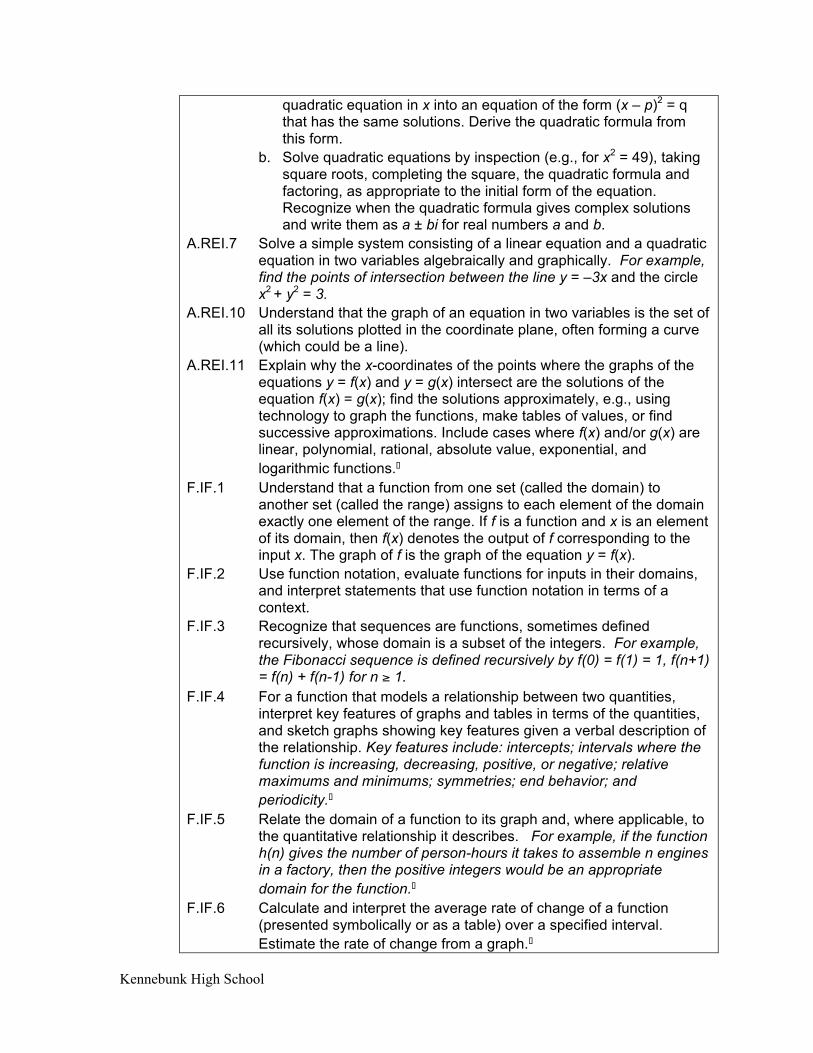
quadratic equation in x into an equation of the form (x – p)2 = q that has the same solutions. Derive the quadratic formula from this form.
b. Solve quadratic equations by inspection (e.g., for x2 = 49), taking square roots, completing the square, the quadratic formula and factoring, as appropriate to the initial form of the equation. Recognize when the quadratic formula gives complex solutions and write them as a ± bi for real numbers a and b.
A.REI.7 Solve a simple system consisting of a linear equation and a quadratic equation in two variables algebraically and graphically. For example, find the points of intersection between the line y = –3x and the circle x2 + y2 = 3.
A.REI.10 Understand that the graph of an equation in two variables is the set of all its solutions plotted in the coordinate plane, often forming a curve (which could be a line).
A.REI.11 Explain why the x-coordinates of the points where the graphs of the equations y = f(x) and y = g(x) intersect are the solutions of the equation f(x) = g(x); find the solutions approximately, e.g., using technology to graph the functions, make tables of values, or find successive approximations. Include cases where f(x) and/or g(x) are linear, polynomial, rational, absolute value, exponential, and logarithmic functions.�
F.IF.1 Understand that a function from one set (called the domain) to another set (called the range) assigns to each element of the domain exactly one element of the range. If f is a function and x is an element of its domain, then f(x) denotes the output of f corresponding to the input x. The graph of f is the graph of the equation y = f(x).
F.IF.2 Use function notation, evaluate functions for inputs in their domains, and interpret statements that use function notation in terms of a context.
F.IF.3 Recognize that sequences are functions, sometimes defined recursively, whose domain is a subset of the integers. For example, the Fibonacci sequence is defined recursively by f(0) = f(1) = 1, f(n+1) = f(n) + f(n-1) for n ≥ 1.
F.IF.4 For a function that models a relationship between two quantities, interpret key features of graphs and tables in terms of the quantities, and sketch graphs showing key features given a verbal description of the relationship. Key features include: intercepts; intervals where the function is increasing, decreasing, positive, or negative; relative maximums and minimums; symmetries; end behavior; and periodicity.�
F.IF.5 Relate the domain of a function to its graph and, where applicable, to the quantitative relationship it describes. For example, if the function h(n) gives the number of person-hours it takes to assemble n engines in a factory, then the positive integers would be an appropriate domain for the function.�
F.IF.6 Calculate and interpret the average rate of change of a function (presented symbolically or as a table) over a specified interval. Estimate the rate of change from a graph.�

Kennebunk High School
F.IF.7 Graph functions expressed symbolically and show key features of the
graph, by hand in simple cases and using technology for more complicated cases.� a. Graph linear and quadratic functions and show intercepts,
maxima, and minima. b. Graph square root, cube root, and piecewise-defined functions,
including step functions and absolute value functions. c. Graph polynomial functions, identifying zeros when suitable
factorizations are available, and showing end behavior. d. (+) Graph rational functions, identifying zeros and asymptotes
when suitable factorizations are available, and showing end behavior.
e. Graph exponential and logarithmic functions, showing intercepts and end behavior, and trigonometric functions, showing period, midline, and amplitude.
F.IF.8 Write a function defined by an expression in different but equivalent forms to reveal and explain different properties of the function. a. Use the process of factoring and completing the square in a
quadratic function to show zeros, extreme values, and symmetry of the graph, and interpret these in terms of a context.
b. Use the properties of exponents to interpret expressions for exponential functions. For example, identify percent rate of change in functions such as y = (1.02)t, y = (0.97)t, y = (1.01)12t, y = (1.2)t/10, and classify them as representing exponential growth or decay.
F.IF.9 Compare properties of two functions each represented in a different way (algebraically, graphically, numerically in tables, or by verbal descriptions). For example, given a graph of one quadratic function and an algebraic expression for another, say which has the larger maximum.
F.BF.2 Write arithmetic and geometric sequences both recursively and with an explicit formula, use them to model situations, and translate between the two forms.�
F.BF.3 Identify the effect on the graph of replacing f(x) by f(x) + k, k f(x), f(kx), and f(x + k) for specific values of k (both positive and negative); find the value of k given the graphs. Experiment with cases and illustrate an explanation of the effects on the graph using technology. Include recognizing even and odd functions from their graphs and algebraic expressions for them.
F.BF.4 Find inverse functions. a. Solve an equation of the form f(x) = c for a simple function f that
has an inverse and write an expression for the inverse. For example, f(x) =2 x3 or f(x) = (x+1)/(x–1) for x ≠1.
b. (+) Verify by composition that one function is the inverse of another.
c. (+) Read values of an inverse function from a graph or a table, given that the function has an inverse.
Kennebunk High School
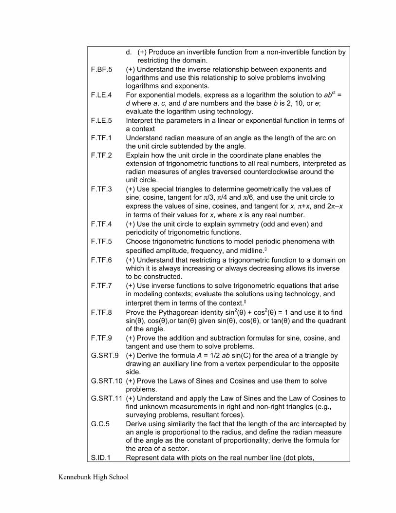
d. (+) Produce an invertible function from a non-invertible function by restricting the domain.
F.BF.5 (+) Understand the inverse relationship between exponents and logarithms and use this relationship to solve problems involving logarithms and exponents.
F.LE.4 For exponential models, express as a logarithm the solution to abct = d where a, c, and d are numbers and the base b is 2, 10, or e; evaluate the logarithm using technology.
F.LE.5 Interpret the parameters in a linear or exponential function in terms of a context
F.TF.1 Understand radian measure of an angle as the length of the arc on the unit circle subtended by the angle.
F.TF.2 Explain how the unit circle in the coordinate plane enables the extension of trigonometric functions to all real numbers, interpreted as radian measures of angles traversed counterclockwise around the unit circle.
F.TF.3 (+) Use special triangles to determine geometrically the values of sine, cosine, tangent for π/3, π/4 and π/6, and use the unit circle to express the values of sine, cosines, and tangent for x, π+x, and 2π–x in terms of their values for x, where x is any real number.
F.TF.4 (+) Use the unit circle to explain symmetry (odd and even) and periodicity of trigonometric functions.
F.TF.5 Choose trigonometric functions to model periodic phenomena with specified amplitude, frequency, and midline.�
F.TF.6 (+) Understand that restricting a trigonometric function to a domain on which it is always increasing or always decreasing allows its inverse to be constructed.
F.TF.7 (+) Use inverse functions to solve trigonometric equations that arise in modeling contexts; evaluate the solutions using technology, and interpret them in terms of the context.�
F.TF.8 Prove the Pythagorean identity sin2(θ) + cos2(θ) = 1 and use it to find sin(θ), cos(θ),or tan(θ) given sin(θ), cos(θ), or tan(θ) and the quadrant of the angle.
F.TF.9 (+) Prove the addition and subtraction formulas for sine, cosine, and tangent and use them to solve problems.
G.SRT.9 (+) Derive the formula A = 1/2 ab sin(C) for the area of a triangle by drawing an auxiliary line from a vertex perpendicular to the opposite side.
G.SRT.10 (+) Prove the Laws of Sines and Cosines and use them to solve problems.
G.SRT.11 (+) Understand and apply the Law of Sines and the Law of Cosines to find unknown measurements in right and non-right triangles (e.g., surveying problems, resultant forces).
G.C.5 Derive using similarity the fact that the length of the arc intercepted by an angle is proportional to the radius, and define the radian measure of the angle as the constant of proportionality; derive the formula for the area of a sector.
S.ID.1 Represent data with plots on the real number line (dot plots,

Kennebunk High School
histograms, and box plots). S.ID.2 Use statistics appropriate to the shape of the data distribution to
compare center (median, mean) and spread (interquartile range, standard deviation) of two or more different data sets.
S.ID.3 Interpret differences in shape, center, and spread in the context of the data sets, accounting for possible effects of extreme data points (outliers).
S.ID.4 Use the mean and standard deviation of a data set to fit it to a normal distribution and to estimate population percentages. Recognize that there are data sets for which such a procedure is not appropriate. Use calculators, spreadsheets, and tables to estimate areas under the normal curve.
S.ID.5 Summarize categorical data for two categories in two-way frequency tables. Interpret relative frequencies in the context of the data (including joint, marginal, and conditional relative frequencies). Recognize possible associations and trends in the data.
S.ID.6 Represent data on two quantitative variables on a scatter plot, and describe how the variables are related. a. Fit a function to the data; use functions fitted to data to solve
problems in the context of the data. Use given functions or choose a function suggested by the context. Emphasize linear and exponential models.
b. Informally assess the fit of a function by plotting and analyzing residuals.
c. Fit a linear function for a scatter plot that suggests a linear association.
S.ID.7 Interpret the slope (rate of change) and the intercept (constant term) of a linear model in the context of the data.
S.ID.8 Compute (using technology) and interpret the correlation coefficient of a linear fit.
S.ID.9 Distinguish between correlation and causation. S.IC.1 Understand statistics as a process for making inferences about
population parameters based on a random sample from that population.
S.IC.2 Decide if a specified model is consistent with results from a given data-generating process, e.g., using simulation. For example, a model says a spinning coin falls heads up with probability 0.5. Would a result of 5 tails in a row cause you to question the model?
S.IC.3 Recognize the purposes of and differences among sample surveys, experiments, and observational studies; explain how randomization relates to each.
S.IC.4 Use data from a sample survey to estimate a population mean or proportion; develop a margin of error through the use of simulation models for random sampling.
S.IC.5 Use data from a randomized experiment to compare two treatments; use simulations to decide if differences between parameters are significant.
S.IC.6 Evaluate reports based on data. S.CP.1 Describe events as subsets of a sample space (the set of outcomes)

Kennebunk High School
using characteristics (or categories) of the outcomes, or as unions, intersections, or complements of other events (“or,” “and,” “not”).
S.CP.2 Understand that two events A and B are independent if the probability of A and B occurring together is the product of their probabilities, and use this characterization to determine if they are independent.
S.CP.3 Understand the conditional probability of A given B as P(A and B)/P(B), and interpret independence of A and B as saying that the conditional probability of A given B is the same as the probability of A, and the conditional probability of B given A is the same as the probability of B.
S.CP.4 Construct and interpret two-way frequency tables of data when two categories are associated with each object being classified. Use the two-way table as a sample space to decide if events are independent and to approximate conditional probabilities. For example, collect data from a random sample of students in your school on their favorite subject among math, science, and English. Estimate the probability that a randomly selected student from your school will favor science given that the student is in tenth grade. Do the same for other subjects and compare the results.
S.CP.5 Recognize and explain the concepts of conditional probability and independence in everyday language and everyday situations. For example, compare the chance of having lung cancer if you are a smoker with the chance of being a smoker if you have lung cancer.
S.CP.6 Find the conditional probability of A given B as the fraction of B’s outcomes that also belong to A, and interpret the answer in terms of the model.
S.CP.7 Apply the Addition Rule, P(A or B) = P(A) + P(B) – P(A and B), and interpret the answer in terms of the model.
S.CP.8 (+) Apply the general Multiplication Rule in a uniform probability model, P(A and B) = P(A)P(B|A) = P(B)P(A|B), and interpret the answer in terms of the model.
S.CP.9 (+) Use permutations and combinations to compute probabilities of compound events and solve problems.
S.MD.1 (+) Define a random variable for a quantity of interest by assigning a numerical value to each event in a sample space; graph the corresponding probability distribution using the same graphical displays as for data distributions.
S.MD.2 (+) Calculate the expected value of a random variable; interpret it as the mean of the probability distribution.
S.MD.3 (+) Develop a probability distribution for a random variable defined for a sample space in which theoretical probabilities can be calculated; find the expected value. For example, find the theoretical probability distribution for the number of correct answers obtained by guessing on all five questions of a multiple-choice test where each question has four choices, and find the expected grade under various grading schemes.
S.MD.4 (+) Develop a probability distribution for a random variable defined for a sample space in which probabilities are assigned empirically; find the expected value. For example, find a current data distribution on

Kennebunk High School
the number of TV sets per household in the United States, and calculate the expected number of sets per household. How many TV sets would you expect to find in 100 randomly selected households?
S.MD.5 (+) Weigh the possible outcomes of a decision by assigning probabilities to payoff values and finding expected values. a. Find the expected payoff for a game of chance. For example, find
the expected winnings from a state lottery ticket or a game at a fast food restaurant.
b. Evaluate and compare strategies on the basis of expected values. For example, compare a high-deductible versus a low-deductible automobile insurance policy using various, but reasonable, chances of having a minor or a major accident.
S.MD.6 (+) Use probabilities to make fair decisions (e.g., drawing by lots, using a random number generator).
S.MD.7 (+) Analyze decisions and strategies using probability concepts (e.g., product testing, medical testing, pulling a hockey goalie at the end of a game).
Resources:
Oxford University Press; Mathemastical Studies standard level course
companion
Released IB Math Studies papers and markschemes
Teacher generated Assessments
Teacher generated Notes