current fluctuations for stochastic particle systems with ... · current fluctuations for...
TRANSCRIPT
SOCIEDADE BRASILEIRA DE MATEMÁTICA ENSAIOS MATEMATICOS
2010, Volume 18, 1–81
Current fluctuations for
stochastic particle systems with
drift in one spatial dimension
Timo Seppalainen
Abstract. This review article discusses limit distributions and variancebounds for particle current in several dynamical stochastic systems of par-ticles on the one-dimensional integer lattice: independent particles, inde-pendent particles in a random environment, the random average process,the asymmetric simple exclusion process, and a class of totally asymmet-ric zero range processes. The first three models possess linear macroscopicflux functions and lie in the Edwards-Wilkinson universality class withscaling exponent 1/4 for current fluctuations. For these we prove Gaus-sian limits for the current process. The latter two systems belong to theKardar-Parisi-Zhang class. For these we prove the scaling exponent 1/3 inthe form of upper and lower variance bounds.
2000 Mathematics Subject Classification: 60K35, 60F05, 60K37.

Acknowledgments
This article is based on lecture notes for a minicourse given at the13th Brazilian School of Probability, August 2-8, 2009, at Maresias, SaoPaulo, and again at the University of Helsinki, Finland, on August 18–20,2009. The author thanks the organizers and the audiences of these twooccasions. The material comes from collaborations with Marton Balazs,Mathew Joseph, Julia Komjathy, Rohini Kumar, Jon Peterson and Fi-ras Rassoul-Agha. The author is grateful for financial support from theNational Science Foundation through grant DMS-0701091 and from theWisconsin Alumni Research Foundation.
Timo Seppalainen

Contents
1 Introduction 7
2 Independent particles executing classical random walks 10
2.1 Model and results . . . . . . . . . . . . . . . . . . . . . . . . 102.2 Sketch of proof . . . . . . . . . . . . . . . . . . . . . . . . . 14
3 Independent particles in a random environment 20
3.1 Model and results . . . . . . . . . . . . . . . . . . . . . . . . 203.2 Sketch of the proof for the quenched mean of the current . 25
4 Random average process 28
4.1 Model and results . . . . . . . . . . . . . . . . . . . . . . . . 284.2 Steps of the proof . . . . . . . . . . . . . . . . . . . . . . . . 30
5 Asymmetric simple exclusion process 41
5.1 Basic properties . . . . . . . . . . . . . . . . . . . . . . . . . 415.2 Results . . . . . . . . . . . . . . . . . . . . . . . . . . . . . . 445.3 Proofs for the identities . . . . . . . . . . . . . . . . . . . . 465.4 A coupling and a random walk bound . . . . . . . . . . . . 495.5 Proof of the upper bound for second class particle moments 545.6 Proof of the lower bound for second class particle moments 61
6 Zero range process 66
6.1 Model and results . . . . . . . . . . . . . . . . . . . . . . . . 666.2 Variance identity . . . . . . . . . . . . . . . . . . . . . . . . 706.3 Coupling for the zero range process . . . . . . . . . . . . . . 71
Bibliography 77


Chapter 1
Introduction
This review article investigates the process of particle current in severalconservative stochastic systems of particles that live on the one-dimensionalinteger lattice. In conservative systems particles are neither created nordestroyed. On the macrosopic, deterministic scale the particle densityρ(t, x) of such systems is governed by a partial differential equation ofscalar conservation law type: ρt + H(ρ)x = 0. The results covered in thisarticle concern the fluctuation behavior of the current, and include someprecise limit results and some coarser order-of-magnitude bounds. Somebackground on advanced probability theory is assumed. For readers withlittle probability background we can also suggest the review article [Sep08]where an attempt was made to explain some of this same material for areader with background in analysis rather than probability.
The particle processes studied fall into two categories. We can definethese two categories by the slope of the flux function H: (i) processes witha linear flux and (ii) those with a strictly concave flux. By definition,the flux H(ρ) is the mean rate at which particle mass moves past a fixedpoint in space when the system is stationary in both space and time andhas overall density ρ of particles. The processes we study are asymmetric
or driven in the sense that the particles have a drift, that is, a preferredaverage direction. This assumption is not necessary for the results forsystems with linear flux, but for those with nonlinear flux it is crucial.
In the statistical physics terminology of surface growth, we can alsolabel these two classes as (i) the EW (Edwards-Wilkinson) and (ii) theKPZ (Kardar-Parisi-Zhang) universality classes [BS]. Surface growth mayseem at first a separate topic from particle systems. But in one dimensionconservative particle systems can be equivalently formulated as interfacemodels. The connection goes by way of regarding the particle occupationnumbers ηi as increments, or discrete gradients, of the interface heightfunction: hi = ηi − ηi−1. Then any movement of particles in the conserva-
7
8 Timo Seppalainen
tive particle system can be equivalently described as deposition or removalof particles from the growing surface. In particular, the current processthen maps directly into the height function.
In the EW class limiting current/height fluctuations are described by thelinear stochastic heat equation Zt = νZxx+W where subscripts are partialderivatives and W represents space-time white noise. In the microscopicmodel the order of magnitude of current fluctuations is n1/4 in terms of ascaling parameter n (n ր ∞) that gives both the space and time scale. Theresults we give describe Gaussian limit distributions of the current process.The examples of systems with linear flux we cover are independent randomwalks, independent random walks in a random environment (RWRE), andthe random average process.
In the RWRE case we in particular wish to understand how the envi-ronment affects the fluctuations. We find a two-level fluctuation picture.On the diffusive n1/2 scale the quenched mean of the current converges toa Brownian motion. Around the quenched mean, on the n1/4 scale, thecurrent converges to the Gaussian processes that arose in the case of inde-pendent classical random walks, but with an additional Brownian randomspatial shift.
The systems with concave flux that we discuss are the asymmetric sim-ple exclusion process (ASEP) and a class of zero range processes. In thiscase the assumption of asymmetry is necessary. We consider only station-ary systems (or small perturbations thereof), and instead of distributionallimits we give only bounds on the variance of the current and on the mo-ments of a second class particle. The current fluctuations are now of ordert1/3. This order of magnitude goes together with superdiffusivity of thesecond class particle whose fluctuations are of order t2/3. Here t is thetime parameter of the process. A separate scaling parameter is not neededsince we have no process level result. These systems are in the KPZ class.
We cannot cover complete proofs for all results to keep this article at areasonable length. The most important result, namely the moment boundsfor the second class particle in ASEP, is proved in full detail, assumingsome basic facts about ASEP.
In some sense interface height in the KPZ class should be described bythe KPZ equation
ht = νhxx − λ(hx)2 + W . (1.1)
However, giving mathematical meaning to this equation has been doneonly indirectly. A formal Hopf-Cole transformation Z = exp(−λν−1h)converts (1.1) into a stochastic heat equation with multiplicative noise:Zt = νZxx +λν−1ZW . The solution of this latter equation is well-defined,and can furthermore be obtained as a limit of an appropriately scaledheight function of a weakly asymmetric simple exclusion process [BG97].Via this link the scaling exponents have recently been verified for the Hopf-

Chapter 1. Introduction 9
Cole solution of the KPZ equation [BQS].The most glaring omission of this article is that we do not treat the
Tracy-Widom fluctuations of KPZ systems such as TASEP (totally asym-metric simple exclusion process), ASEP or the PNG (polynuclear growth)model. In the ASEP section we only state briefly the Ferrari-Spohn theo-rem [FS06] on the limit distribution of the current across a characteristicin stationary TASEP. This area is advancing rapidly and requires a re-view article of its own if any degree of detail is to be covered. Tracy andWidom have recently written a series of papers where the fluctuation limitsoriginally proved for TASEP by Johansson [Joh00] have been extended toASEP [TW08a, TW08b, TW09a, TW09b, TW10]. Another line of recentwork extends the TASEP limits to more general space-time points andinitial distributions [BFP, CFP].
A notational convention. Z+ = 0, 1, 2, 3, . . . and N = 1, 2, 3, . . . .

Chapter 2
Independent particles
executing classical
random walks
2.1 Model and results
Fix a probability distribution p(x) on Z. Let us assume for simplicity thatp(x) has finite range, that is,
the set x ∈ Z : p(x) > 0 is finite. (2.1)
For each site x ∈ Z and index k ∈ N let Xx,k
be a discrete-time randomwalk with initial point Xx,k
0 = x and transition probability
P (Xx,ks+1 = y |Xx,k
s = z) = p(y − z)
for times s ∈ Z+ and space points z, y ∈ Z. The walks Xx,k
: x ∈ Z, k ≥1 are independent of each other. Let
v =∑
x∈Z
xp(x) and σ21 =
∑
x∈Z
(x − v)2p(x)
be the mean speed and variance of the walks.At time 0 we start a random number ηx(0) of particles at site x. The
assumption is that the initial occupation variables η(0) = ηx(0) : x ∈ Zare i.i.d. (independent and identically distributed) with finite mean andvariance
µ0 = E[ηx(0)] and σ20 = Var[ηx(0)]. (2.2)
10
Chapter 2. Independet particles executing classical random walks 11
Furthermore, the variables ηx(0) and the walks Xx,k
are independentof each other. If the locations of individual particles are not of interest butonly the overall particle distribution, the particle configuration at times ∈ N is described by the occupation variables η(s) = ηx(s) : x ∈ Zdefined as
ηx(s) =∑
y∈Z
η0(y)∑
k=1
1Xy,ks = x.
A basic fact is that if the initial occupation variables are i.i.d. Poissonwith common mean µ, then so are the occupation ηx(s) : x ∈ Z at anyfixed time s ∈ Z+. This invariance follows easily from basic properties ofPoisson distributions: the counts of particles that move from x to y areindependent Poisson variables across all pairs (x, y).
Let Eµ denote expectation under the stationary process with mean µoccupations. The flux function is the expected rate of flow in the stationaryprocess:
H(µ) = Eµ[net number of particles that jump across edge (0, 1)
left to right in one time step]
= Eµ
[ ∑
x≤0
η0(x)∑
k=1
1Xx,k1 ≥ 1 −
∑
x>0
η0(x)∑
k=1
1Xx,k1 ≤ 0
]
= vµ.
(2.3)
The linear flux puts this system in the class where we expect n1/4 mag-nitude current fluctuations. Next we define the current process and theGaussian process that describes the limit.
Let n ∈ N denote a scaling parameter that eventually goes to ∞. For(macroscopic) times t ∈ R+ and a spatial variable r ∈ R, let
Yn(t, r) = Yn,1(t, r) − Yn,2(t, r) (2.4)
with
Yn,1(t, r) =∑
x≤0
ηx(0)∑
k=1
1Xx,k⌊nt⌋ > ⌊ntv⌋ + r
√n (2.5)
and
Yn,2(t, r) =∑
x>0
ηx(0)∑
k=1
1Xx,k⌊nt⌋ ≤ ⌊ntv⌋ + r
√n . (2.6)
The variable Yn(t, r) represents the net left-to-right current of particlesseen by an observer who starts at the origin and reaches point ⌊ntv⌋ +⌊r√n⌋ in time ⌊nt⌋. Its mean is
EYn(t, r) = µ0E(X⌊nt⌋ − ⌊ntv⌋ − ⌊r√n ⌋
)= −µ0r
√n + O(1).
12 Timo Seppalainen
Define the centered and appropriately scaled process by
Y n(t, r) = n−1/4(Yn(t, r) − EYn(t, r)
).
The goal is to prove a limit for the joint distributions of these randomvariables. We will not tackle process-level convergence. But let us pointout that there is a natural path space D2 of functions of two parameters(t, r) that contains the paths of the processes Yn. Elements of D2 arecontinuous from above with limits from below in a suitable way, and thereis a metric that generalizes the standard Skorohod topology of the usualD-space of cadlag paths. (See [BW71, Kum08].)
Let
ϕν2(x) =1√
2πν2exp
(− x2
2ν2
)and Φν2(x) =
∫ x
−∞ϕν2(y)dy (2.7)
denote the centered Gaussian density with variance ν2 and its distributionfunction. Let W be a two-parameter Brownian motion on R+×R and B atwo-sided one-parameter Browian motion on R. W and B are independent.Define the process Z by
Z(t, r) =√
µ0
∫∫
[0,t]×R
ϕσ21(t−s)(r − x) dW (s, x)
+ σ0
∫
R
ϕσ21t(r − x)B(x) dx.
(2.8)
Z(t, r) : t ∈ R+, r ∈ R is a mean zero Gaussian process. Its covariancecan be expressed as follows: with
Ψν2(x) = ν2ϕν2(x) − x(1 − Φν2(x)
)(2.9)
define
Γ1
((s, q), (t, r)
)= Ψσ2
1(t+s)(r − q) − Ψσ21 |t−s|(r − q) (2.10)
and
Γ2
((s, q), (t, r)
)= Ψσ2
1s(−q) + Ψσ21t(r) − Ψσ2
1(t+s)(r − q). (2.11)
Then
E[Z(s, q)Z(t, r)] = µ0Γ1
((s, q), (t, r)
)+ σ2
0Γ2
((s, q), (t, r)
). (2.12)
Remark 2.1. Some comments on Gaussian processes defined above. Com-parison of (2.8) and (2.12) shows that Γ1 is the covariance of the dynamicalfluctuations represented by the space-time white noise dW -integral, and Γ2

Chapter 2. Independet particles executing classical random walks 13
is the covariance of the contribution of the initial fluctuations representedby the Brownian motion σ0B(·).
Γ1 has this alternative formula:
Γ1
((s, q), (t, r)
)= 1
2
∫ σ21(t+s)
σ21 |t−s|
1√2πv
exp 1
2v(r − q)2
dv. (2.13)
To verify that the process
ζ(t, r) =
∫∫
[0,t]×R
ϕσ21(t−s)(r − x) dW (s, x)
has covarianceEζ(s, q)ζ(t, r) = Γ1
((s, q), (t, r)
)(2.14)
is straightforward from the general property that for f, g ∈ L2(Rd) thewhite-noise integrals
∫f dW and
∫g dW on R
d are by definition meanzero Gaussian random variables that satisfy
E[(∫
f dW)(∫
g dW)]
=
∫
Rd
f(x)g(x) dx.
To say that B(x) is a (standard) two-sided Brownian motion means thatwe take two independent standard Brownian motions B1 and B2 and set
B(x) =
B1(x), x ≥ 0
B2(−x), x < 0.
To show that the process
ξ(t, r) =
∫
R
ϕσ21t(r − x)B(x) dx
is a mean-zero Gaussian process with covariance
Eξ(s, q)ξ(t, r) = Γ2
((s, q), (t, r)
)
this formula is useful: if f, g are absolutely continuous functions on R+
such that xf(x) → 0 and xg(x) → 0 as x → ∞, then
∫∫
R2+
f ′(x)g′(y)(x ∧ y) dx dy =
∫ ∞
0
f(x)g(x) dx.
It is also the case that the process Z(t, r) is the unique weak solution ofthe following initial value problem for a linear stochastic heat equation onR+ × R:
Zt =σ21
2 Zrr +√
µ0 W , Z(0, r) = σ0B(r).

14 Timo Seppalainen
(Above, subscript means partial derivative.) A weak solution of this equa-tion is defined by the requirement
∫
R
φ(r)Z(t, r) dr − σ0
∫
R
φ(r)B(r) dr
=σ21
2
∫∫
[0,t]×R
φ′′(r)Z(s, r) dr ds +√
µ0
∫∫
[0,t]×R
φ(r)dW (s, r)
for all φ ∈ C∞c (R) (compactly supported, infinitely differentiable). See the
lecture notes of Walsh [Wal86].
We can now state the main result.
Theorem 2.2. Assume the initial occupation variables are i.i.d. with finitemean and variance as in (2.2). Then as n → ∞, the finite-dimensionaldistributions of the process Y n(t, r) : (t, r) ∈ R+ × R converge weaklyto the finite-dimensional distributions of the mean zero Gaussian processZ(t, r) : (t, r) ∈ R+ × R.
The statement means that for any space-time points (t1, r1), . . . , (tk, rk),this weak convergence of R
k-valued random vectors holds:
(Y n(t1, r1), . . . , Y n(tk, rk))D−→ (Z(t1, r1), . . . , Z(tk, rk)).
Under additional moment assumptions process level convergence in thespace D2 can be proved (see [Kum08]). We state a corollary for the spe-cial case of the stationary occupation process η(t). Its proof comes fromsimplifying expression (2.12) for the covariance.
Corollary 2.1. Suppose the process is stationary so that ηx(t) : x ∈ Zare i.i.d. Poisson with mean µ0 for each fixed t. Then at r = 0 the limitprocess Z has covariance
EZ(s, 0)Z(t, 0) =µ0σ1√
2π
(√s +
√t −
√|t − s|
).
In other words, process Z(·, 0) is fractional Brownian motion with Hurstparameter 1/4.
2.2 Sketch of proof
We turn to discuss the proof of Theorem 2.2. Independent walks allowus to compute everything in a straightforward manner. Fix some N ∈ N,time points 0 < t1 < t2 < · · · < tN ∈ R+, space points r1, r2, . . . , rN ∈ R
and an N -vector θ = (θ1, . . . , θN ) ∈ RN . Form the linear combinations
Y n(θ) =
N∑
i=1
θiY n(ti, ri) and Z(θ) =
N∑
i=1
θiZ(ti, ri).
Chapter 2. Independet particles executing classical random walks 15
The goal is now to prove
Proposition 2.1.
E[exp
iY n(θ)
]→ E
[exp
iZ(θ)
]. (2.15)
Since the random walks and initial occupation variables are independent,we can write Y n(θ) as a sum of independent random variables and takeadvantage of standard central limit theorems from the literature.
Y n(θ) = n− 14
N∑
i=1
θi
Yn(ti, ri) − EYn(ti, ri)
= Wn =
∞∑
m=−∞u(m) (2.16)
with
u(m) =
N∑
i=1
θi
(Um(ti, ri)1m ≤ 0 − Vm(ti, ri)1m > 0
), (2.17)
and
Um(t, r) = n− 14
ηm(0)∑
j=1
1Xm,jnt > ⌊ntv⌋ + r
√n
− n− 14 µ0P (Xm
nt > ⌊ntv⌋ + r√
n ),
(2.18)
Vm(t, r) = n− 14
ηm(0)∑
j=1
1Xm,jnt ≤ ⌊ntv⌋ + r
√n
− n− 14 µ0P (Xm
nt ≤ ⌊ntv⌋ + r√
n ).
The variables u(m)m∈Z are independent because initial occupation vari-ables and walks are independent.
Let a(n) ր ∞ be a sequence that will be determined precisely in theproof. As the first step we observe that the terms |m| > a(n)
√n can be
discarded from (2.16). Define
W ∗n =
∑
|m|≤a(n)√
n
u(m). (2.19)
The lemma below is proved by calculating moments of the random walks.
Lemma 2.1. E|Wn − W ∗n |2 → 0 as n → ∞.
16 Timo Seppalainen
The limit Z(θ) in our goal (2.15) has N (0, σ(θ)2) distribution withvariance
σ(θ)2 =∑
1≤i,j≤N
θiθj
[µ0Γ1
((ti, ri), (tj , rj)
)+σ2
0Γ2
((ti, ri), (tj , rj)
)]. (2.20)
The two Γ-terms, defined earlier in (2.10) and (2.11), have the followingexpressions in terms of a standard 1-dimensional Brownian motion Bt:
Γ1
((s, q), (t, r)
)=
∫ ∞
−∞
(P[Bσ2
1s ≤ q − x]P[Bσ21t > r − x]
− P[Bσ21s ≤ q − x,Bσ2
1t > r − x])
dx
(2.21)
and
Γ2
((s, q), (t, r)
)=
∫ 0
−∞P[Bσ2
1s > q − x]P[Bσ21t > r − x] dx
+
∫ ∞
0
P[Bσ21s ≤ q − x]P[Bσ2
1t ≤ r − x] dx.
(2.22)
Remark 2.3. Turning formulas (2.21)–(2.22) into (2.10)–(2.11) involvescalculus and these properties of Gaussians: (d/dx)Ψν2(x) = −Φν2(−x),Φν2(x) = 1 − Φν2(−x) and
∫ ∞
−∞Φα2(x)Φν2(r − x) dx =
∫ r
−∞Φα2+ν2(x) dx.
By Lemma 2.1, the desired limit (2.15) follows from showing
E(eiW∗n ) → e−σ(θ)2/2. (2.23)
This will be achieved by the Lindeberg-Feller theorem.
Theorem 2.4 (Lindeberg-Feller). For each n, suppose Xn,j : 1 ≤ j ≤J(n) are independent, mean-zero, square-integrable random variables andlet Sn = Xn,1 + · · · + Xn,J(n). Assume that
limn→∞
J(n)∑
j=1
E(X2n,j) = σ2
and for each ε > 0,
limn→∞
J(n)∑
j=1
E(X2
n,j1|Xn,j | ≥ ε)
= 0.
Chapter 2. Independet particles executing classical random walks 17
Then as n → ∞, Sn converges in distribution to a N (0, σ2)-distributedGaussian random variable. In terms of probabilities, the conclusion is thatfor all s ∈ R,
limn→∞
PSn ≤ s =1√
2πσ2
∫ s
−∞e−x2/2σ2
dx.
In terms of characteristic functions, the conclusion is that for all t ∈ R,
limn→∞
E(eitSn) = e−σ2t2/2.
Now to prove (2.23) the task is to verify the conditions of the Lindeberg-Feller theorem: ∑
|m|≤a(n)√
n
E(u(m)2) → σ(θ)2 (2.24)
and ∑
|m|≤a(n)√
n
E(|u(m)|21|u(m)| ≥ ε
)→ 0. (2.25)
We begin with the negligibility condition (2.25). This will determinea(n).
Lemma 2.2. Under assumption (2.2),
limn→∞
∑
|m|≤a(n)√
n
E(|u(m)|21|u(m)| ≥ ε
)= 0. (2.26)
Proof. Since|u(m)| ≤ Cn−1/4
(ηm(0) + µ0
),
for a different ε1 > 0 and by shift-invariance,∑
|m|≤a(n)√
n
E[|u(m)|21|u(m)| ≥ ε
]
≤ Ca(n)E[(η0(0) + µ0)
21η0(0) ≥ n1/4ε1].
By the moment assumption (2.2) this last expression → 0 for every ε1 > 0if a(n) ր ∞ slowly enough, for example
a(n) =(E
[(η0(0) + µ0)
21η0(0) ≥ n1/8])−1/2
.
We turn to checking (2.24).∑
|m|≤a(n)√
n
E[u(m)2
]
=∑
1≤i,j≤N
θiθj
∑
|m|≤a(n)√
n
[1m≤0 E
(Um(ti, ri)Um(tj , rj)
)
+ 1m>0 E(Vm(ti, ri)Vm(tj , rj)
)].
(2.27)

18 Timo Seppalainen
To the expectations we apply this formula for the covariance of two randomsums: with Zi i.i.d. and independent of a random K ∈ Z+,
Cov( K∑
i=1
f(Zi) ,
K∑
j=1
g(Zj))
= EK Cov(f(Z), g(Z)) + Var(K)Ef(Z)Eg(Z).
(2.28)
For the first expectation on the right in (2.27):
E(Um(s, q)Um(t, r)
)
= n−1/2 Cov
( ηm(0)∑
j=1
1Xm,jns > ⌊nsv⌋ + q
√n ,
ηm(0)∑
j=1
1Xm,jnt > ⌊ntv⌋ + r
√n
)
= n−1/2µ0
[P (Xm
ns > ⌊nsv⌋ + q√
n, Xmnt > ⌊ntv⌋ + r
√n )
− P (Xmns > ⌊nsv⌋ + q
√n )P (Xm
nt > ⌊ntv⌋ + r√
n )]
+ n−1/2σ20P (Xm
ns > ⌊nsv⌋ + q√
n )P (Xmnt > ⌊ntv⌋ + r
√n ).
Do the same for the V -terms. After some rearranging of the probabilities,we arrive at
∑
|m|≤a(n)√
n
E[u(m)2
](2.29)
= n−1/2∑
1≤i,j≤N
θiθj
[µ0
∑
|m|≤a(n)√
n
P (Xm
nti≤ ⌊ntiv⌋ + ri
√n ) (2.30)
× P (Xmntj
> ⌊ntjv⌋ + rj
√n )
− P (Xmnti
≤ ⌊ntiv⌋ + ri
√n, Xm
ntj> ⌊ntjv⌋ + rj
√n )
+ σ20
∑
−a(n)√
n≤m≤0
P (Xmnti
> ⌊ntiv⌋ + ri
√n )P (Xm
ntj> ⌊ntjv⌋ + rj
√n )
+ σ20
∑
0<m≤a(n)√
n
P (Xmnti
≤ ⌊ntiv⌋ + ri
√n )P (Xm
ntj≤ ⌊ntjv⌋ + rj
√n )
].
The terms above have been arranged so that the sums match up withthe integrals in (2.20)–(2.22). Limit (2.24) now follows because each sum
Chapter 2. Independet particles executing classical random walks 19
converges to the corresponding integral. To illustrate with the last term,the convergence needed is
n−1/2∑
0<m≤a(n)√
n
P (Xmns ≤ ⌊nsv⌋ + q
√n )P (Xm
nt ≤ ⌊ntv⌋ + r√
n )
=n−1/2∑
0<m≤a(n)√
n
PXns−⌊nsv⌋√
n≤ q− m√
n
× PXnt−⌊ntv⌋√
n≤r − m√
n
−→n→∞
∫ ∞
0
P[Bσ21s ≤ q − x]P[Bσ2
1t ≤ r − x] dx.
(2.31)
This follows from the CLT, a Riemann sum type argument and some esti-mation. We skip the details. With this we consider Theorem 2.2 proved.
References
The results for i.i.d. walks appeared, with a slightly different definitionof the current process, in [Sep05] and [Kum08]. Earlier related resultsappeared in [DGL85].

Chapter 3
Independent particles in a
random environment
In this chapter we generalize the results of Chapter 2 to particles in arandom environment, with the purpose of seeing how the environment in-fluences the outcome. In a fixed environment, that is, conditional on theenvironment, the particles evolve independently. But under the joint dis-tribution of the walks and the environment, the particles are no longerindependent because their evolution gives information about the environ-ment. The environment is static, which means that it is fixed in time.
3.1 Model and results
We formulate the standard one-dimensional nearest-neighbor random walkin random environment (RWRE) model and then put many particles ina fixed environment. We describe the (known) law of large numbers andcentral limit theorem of the walk itself, and then the (newer) results oncurrent fluctuations for many particles.
The space of environments is Ω = [0, 1]Z. For an environment ω =ωxx∈Z ∈ Ω let Xm,i
m,i be a family of Markov chains on Z with distri-bution Pω determined by the following properties:
1. Xm,i
m∈Z,i∈N are independent under the measure Pω.
2. Pω(Xm,i0 = m) = 1, for all m ∈ Z and i ∈ N.
3. Each walk obeys these transition probabilities:
Pω(Xm,in+1 = x+1|Xm,i
n = x) = 1−Pω(Xm,in+1 = x−1|Xm,i
n = x) = ωx.
20
Chapter 3. Independet particles in a random environment 21
A system of random walks in a random environment may then be con-structed by first choosing an environment ω according to a probabilitydistribution P on Ω and then constructing the system of random walksXm,i
as described above. The distribution Pω of the random walksgiven the environment ω is called the quenched distribution. The aver-aged distribution P (also called annealed) is obtained by averaging thequenched law over all environments: P(·) =
∫Ω
Pω(·)P (dω). Expectationswith respect to the measures P , Pω and P are denoted by EP , Eω, and E,respectively, and variances with respect to the measure Pω will be denotedby Varω. We make the following assumptions on the environment.
Assumption 1. The distribution P on environments is i.i.d. and uni-formly elliptic. That is, ωxx∈Z are i.i.d. under the measure P , andthere exists a κ > 0 such that P (ωx ∈ [κ, 1 − κ]) = 1. Furthermore,EP (ρ2+ε0
0 ) < 1 for some ε0 > 0, where ρx = (1 − ωx)/ωx.
These assumptions put the RWRE in the regime where it has transienceto +∞ with a strictly positive speed and also satisfies a CLT with anenvironment-dependent centering. We summarize these results here. De-fine a shift map on environments by (θxω)y = ωx+y. Let T1 = infn ≥ 0 :Xn = 1 be the first hitting time of site 1 ∈ Z by a RWRE started at theorigin, and define
Znt(ω) = vP
⌊ntvP ⌋−1∑
i=0
(Eθiω(T1) − ET1). (3.1)
The asymptotic speed vP is defined in the first statement of the nexttheorem where we summarize some known basic facts about RWRE.
Theorem 3.1 ([Sol75, Pet08, Zei04]). Under the assumptions made abovewe have these conclusions.
1. The RWRE satisfies a law of large numbers with positive speed. Thatis,
limn→∞
Xn
n=
1 − EP (ρ0)
1 + EP (ρ0)≡ vP > 0, P-a.s. (3.2)
2. The RWRE satisfies a quenched functional central limit theorem withan environment-dependent centering. Let
Bn(t) =Xnt − ntvP + Znt(ω)
σ1√
n, where σ2
1 = v3P EP (Varω T1).
Then, for P -a.e. environment ω, under the quenched measure Pω,Bn(·) converges weakly to standard Brownian motion as n → ∞.
22 Timo Seppalainen
3. Let
ζn(t) =Znt(ω)
σ2√
n, where σ2
2 = v2P Var(EωT1).
Then, under the measure P on environments, ζn(·) converges weaklyto standard Brownian motion as n → ∞.
4. The RWRE satisfies an averaged central limit theorem. Let
Bn(t) =
Xnt − ntvP
σ√
n, where σ2 = σ2
1 + σ22 .
Then, under the averaged measure P, Bn(·) converges weakly to stan-
dard Brownian motion.
The requirement that EP (ρ20) < 1 cannot be relaxed in order for the
CLT to hold [KKS75, PZ09]. Centering by ntvP −Znt(ω) in the quenchedCLT is the same as centering by the quenched mean on account of thisbound:
limn→∞
P
ω : supk≤n
|Eω(Xk) − kvP + Zk(ω)| ≥ ε√
n
= 0, ∀ε > 0. (3.3)
But Znt(ω) is more convenient because it is a sum of stationary, ergodicrandom variables.
These properties of the walk are sufficient for describing the current fluc-tuations. Assumptions on the initial occupation variables η(0) = ηx(0)are similar to those in the previous section. We will allow the distribu-tion of η(0) to depend on the environment (in a measurable way), and weassume a certain stationarity.
Assumption 2. Given the environment ω, variables ηx(0) are inde-pendent and independent of the random walks. The conditional distribu-tion of ηx(0) given ω is denoted by Pω(ηx(0) = k), and these measurablefunctions of ω satisfy Pω(ηx(0) = k) = Pθxω(η0(0) = k). Also, for someε0 > 0,
EP [Eω(ηx(0))2+ε0 + Varω(ηx(0))2+ε0 ] < ∞. (3.4)
Let
µ0 = EP [Eω(ηx(0))] = E[ηx(0)] and σ20 = EP [Varω(ηx(0))] .
The current is defined as before:
Yn(t, r) =∑
m≤0
ηm(0)∑
k=1
1Xm,knt > ⌊ntvP ⌋ + r
√n
−∑
m>0
ηm(0)∑
k=1
1Xm,knt ≤ ⌊ntvP ⌋ + r
√n .
(3.5)
Chapter 3. Independet particles in a random environment 23
Now for the results, beginning with the quenched mean of the current.This turns out to essentially follow the correction Znt(ω) of the quenchedCLT, which is of order
√n. Assumptions 1 and 2 are in force for all the
results that follow.
Theorem 3.2. For any ε > 0, 0 < R,T < ∞,
limn→∞
Pω : sup
t∈[0,T ]r∈[−R,R]
∣∣EωYn(t, r)+µ0r√
n+µ0Znt(ω)∣∣ ≥ ε
√n
= 0. (3.6)
Consequently the two-parameter process n−1/2EωYn(t, r) : t ∈ R+, r ∈R converges weakly to −µ0r + µ0σ2W (t) : t ∈ R+, r ∈ R where W (·)is a standard Brownian motion.
Next we center the current at its quenched mean by defining
Vn(t, r) = Yn(t, r) − Eω[Yn(t, r)].
The fluctuations of Vn(t, r) are of order n1/4 and similar to the current fluc-tuations of classical walks from the previous section. Recall the definitionsof Γ1 and Γ2 from (2.10)–(2.11) and abbreviate
Γ((s, q), (t, r)
)= µ0Γ1
((s, q), (t, r)
)+ σ2
0Γ2
((s, q), (t, r)
). (3.7)
Let (V,Z) = (V (t, r), Z(t) : t ∈ R+, r ∈ R) be the process whose jointdistribution is defined as follows:
(i) Marginally, Z(·) = σ2W (·) for a standard Brownian motion W (·).
(ii) Conditionally on the path Z(·) ∈ C(R+, R), V is the mean zeroGaussian process indexed by R+ × R with covariance
E[V (s, q)V (t, r) |Z(·)] = Γ((s, q + Z(s)), (t, r + Z(t))
)(3.8)
for (s, q), (t, r) ∈ R+ × R. An equivalent way to say this is to first takeindependent (V 0, Z) with Z as above and V 0 = V 0(t, r) : (t, r) ∈ R+×Rthe mean zero Gaussian process with covariance Γ
((s, q), (t, r)
)from (3.7),
and then define V (t, r) = V 0(t, r + Z(t)).
Theorem 3.3. Under the averaged probability P, as n → ∞, the finite-dimensional distributions of the joint process
(n−1/4Vn(t, r),n−1/2Znt(ω)) :
t ∈ R+, r ∈ R
converge to those of the process (V,Z).
Thus up to a random shift of the spatial argument we see the same limitprocess as for classical walks: the process V (t, r) = V (t, r−Z(t)) is a mean
24 Timo Seppalainen
zero Gaussian process with covariance E[V (s, q)V (t, r)] = Γ((s, q), (t, r)
)
from (3.7).As for classical walks, let us look at the stationary case. The invariant
distribution is now valid under a fixed ω: the ηx(0) are independent and
ηx(0) ∼ Poisson(µ0f(θxω)), where f(ω) =vP
ω0
(1 +
∞∑
i=1
i∏
j=1
ρj
). (3.9)
In this case, Eωη0(0) = Varω η0(0) = µ0f(ω). By Assumption 1 EP (ρ2+ε0 )
< 1 for some ε > 0, and from that it can be shown that EP [f(ω)2+ε] < ∞.Therefore Assumption 2 holds. One can also check that, as for classicalwalks in (2.3), in this stationary situation the flux is linear: H(µ0) = µ0vP .
Recall from Corollary 2.1 that for classical random walks the limit pro-cess (with fixed space variable r) in the case µ0 = σ2
0 is fractional Brownianmotion ξ with covariance
E[ξ(s)ξ(t)] =µ0σ1√
2π(√
s +√
t −√
|s − t| ).
For RWRE, µ0 = σ20 implies that
E[V (s, 0)V (t, 0) |Z(·)]= µ0
[Ψσ2
1s(−Z(s)) + Ψσ21t(Z(t)) − Ψσ2
1 |s−t|(Z(t) − Z(s))].
(3.10)
Since the right hand side of (3.10) is a non-constant random variable, themarginal distribution of V (t, 0) is non-Gaussian. Taking expectations of(3.10) with respect to Z(·) gives that
E[V (s, 0)V (t, 0)] =µ0
√σ2
1 + σ22√
2π(√
s +√
t −√
|s − t|). (3.11)
Thus we get this conclusion: if µ0 = σ20 for RWRE then the limit process
V (·, 0) has the same covariance as fractional Brownian motion, but it isnot a Gaussian process.
As the reader may have surmised, we can remove the random shift Zfrom the limit process V by introducing the environment-dependent shiftin the current process itself. We state this result too. For (t, r) ∈ R+ × R
define
Y (q)n (t, r) =
∑
m>0
ηm(0)∑
k=1
1Xm,knt ≤ ntvP − Znt(ω) + r
√n
−∑
m≤0
ηm(0)∑
k=1
1Xm,knt > ntvP − Znt(ω) + r
√n
(3.12)
Chapter 3. Independet particles in a random environment 25
and its centered version
V (q)n (t, r) = Y (q)
n (t, r) − EωY (q)n (t, r).
The process V(q)n has the same limit as classical random walks. Let V 0 =
V 0(t, r) : (t, r) ∈ R+ × R be the mean zero Gaussian process withcovariance Γ
((s, q), (t, r)
)from (3.7).
Theorem 3.4. Under the averaged probability P, as n → ∞, the finite-
dimensional distributions of the joint process(n−1/4V
(q)n (t, r),n−1/2Znt(ω)):
t ∈ R+, r ∈ R
converge to those of the process (V 0, Z) where V 0 and Zare independent.
3.2 Sketch of the proof for the quenched mean
of the current
The basic thrust of the proof of Theorem 3.3 for the limit of the centeredcurrent is similar to the one outlined in Section 2.2 for classical randomwalks. The differences lie in the technical details needed to handle therandom environment. So we omit further discussion of that theorem andof the related Theorem 3.4. In this section we explain the main ideasbehind the proof of Theorem 3.2 for the quenched mean of the current. Toput aside inessential detail we drop the uniformity, fix (t, r), and sketchinformally the argument for the following simplified statement:
Proposition 3.1. For any ε > 0,
limn→∞
P
ω :∣∣EωYn(t, r) + µ0r
√n + µ0Znt(ω)
∣∣ ≥ ε√
n
= 0. (3.13)
This proceeds via a sequence of estimations. Abbreviate the centeredquenched mean by
Wn = EωYn(t, r) + µ0r√
n
=∑
m≤0
Eω[η0(m)]Pω(Xmnt > ntvP + r
√n )
−∑
m>0
Eω[η0(m)]Pω(Xmnt ≤ ntvP + r
√n ) + µ0r
√n.
For a suitable sequence a(n) ր ∞ define
Wn =0∑
m=−⌊a(n)√
n⌋+1
Eω(η0(m))Φσ21t
(−Znt(θ
mω) − m√n
− r
)
−⌊a(n)
√n⌋∑
m=1
Eω(η0(m))Φσ21t
(Znt(θ
mω) − m√n
+ r
)+ µ0r
√n.
26 Timo Seppalainen
The quenched CLT (part 2 of Theorem 3.1) implies that the difference
supx∈R
∣∣∣∣Pω
(Xn − nvP + Zn(ω)√
n≤ x
)− Φσ2
1(x)
∣∣∣∣
vanishes P -a.s. as n → ∞. Thus it is possible to choose a(n) ր ∞ slowlyenough so that
limn→∞
P
(1√n
∣∣∣Wn − Wn
∣∣∣ ≥ ε
)= 0. (3.14)
The next step is to remove the shifts from Znt by defining
Wn =0∑
m=−⌊a(n)√
n⌋+1
Eω(η0(m))Φσ21t
(−Znt(ω) − m√
n− r
)
−⌊a(n)
√n⌋∑
m=1
Eω(η0(m))Φσ21t
(Znt(ω) − m√
n+ r
)+ µ0r
√n.
The estimation
limn→∞
P
(1√n
∣∣∣Wn − Wn
∣∣∣ ≥ ε
)= 0 (3.15)
follows from representation (3.1) of Znt as a sum of ergodic terms whosebehavior is well understood.
Subsequently the ergodicity of the environment allows us to average thequenched means Eω(η0(m)) and replace Wn with
Wn =
0∑
m=−⌊a(n)√
n⌋+1
µ0Φσ21t
(−Znt(ω) − m√
n− r
)
−⌊a(n)
√n⌋∑
m=1
µ0Φσ21t
(Znt(ω) − m√
n+ r
)+ µ0r
√n.
After this, replace the sums with integrals to approximate n−1/2Wn
with
µ0r − µ0
∫ a(n)
0
Φσ21t
(Znt(ω)√
n+ r − x
)− Φσ2
1t
(−Znt(ω)√
n− r − x
)dx.
A calculus exercise shows that
∫ A
0
Φα2 (z − x) − Φα2 (−z − x) dx = z + Ψα2(A + z) − Ψα2(A − z),
Chapter 3. Independet particles in a random environment 27
where Ψα2(x) is again the function defined in (2.9). Therefore,
∫ a(n)
0
Φσ21t
(Znt(ω)√
n+ r − x
)− Φσ2
1t
(−Znt(ω)√
n− r − x
)dx
=Znt(ω)√
n+ r + Ψσ2
1t
(a(n) +
Znt(ω)√n
+ r
)
− Ψσ21t
(a(n) − Znt(ω)√
n− r
).
The last two terms vanish as n → ∞ because Ψσ21t(∞) = 0 and n−1/2Znt
is tight by part 3 of Theorem 3.1.Collecting the steps (and taking the omitted details on faith) leads to
the estimate
Wn = −µ0Znt + o(√
n ) in probability
as was claimed in (3.13).
References
The results for the current of RWRE’s are from [PS]. Zeitouni’s lecturenotes [Zei04] are a standard reference for background on RWRE.
Chapter 4
Random average process
4.1 Model and results
The state of the random average process (RAP) is a height function σ :Z → R where the value σ(i) can be thought of as the height of an interfaceabove site i. The state evolves in discrete time according to the followingrule. At each time point s = 1, 2, 3, . . . and at each site k ∈ Z, a randomprobability vector ωk,s = (ωk,s(j) : −R ≤ j ≤ R) of length 2R + 1 isdrawn. Given the state σs−1 = (σs−1(i) : i ∈ Z) at time s − 1, at time sthe height value at site k is updated to
σs(k) =∑
j:|j|≤R
ωk,s(j)σs−1(k + j). (4.1)
This update is performed independently at each site k to form the stateσs = (σs(k) : k ∈ Z) at time s. The weight vectors ωk,sk∈Z,s∈N arei.i.d. across space-time points (k, s). This system was originally studiedby Ferrari and Fontes [FF98].
Letp(0, j) = E[ω0,0(j)]
denote the averaged weights with mean and variance
V =∑
x
x p(x) and σ21 =
∑
x∈Z
(x − V )2 p(0, x). (4.2)
Let b = −V .Make two nondegeneracy assumptions on the distribution of the weight
vectors.(i) There is no integer h > 1 such that, for some x ∈ Z,
∑
k∈Z
p(0, x + kh) = 1.
28
Chapter 4. Random average process 29
This is also expressed by saying that the span of the random walk withjump probabilities p(0, j) is 1 [Dur04, page 129]. It follows that the additivegroup generated by x ∈ Z : p(0, x) > 0 is all of Z, in other words thiswalk is aperiodic in Spitzer’s terminology [Spi76].
(ii) Second, we assume that
Pmaxj
ω0,0(j) < 1 > 0. (4.3)
Let σs be a random average process normalized by σ0(0) = 0 and whoseinitial increments ηi(0) = σ0(i) − σ0(i − 1) : i ∈ Z are i.i.d. such that
there exists α > 0 such that E[ |ηi(0)|2+α ] < ∞. (4.4)
As before, the mean and variance of initial increments are
µ0 = E(ηi(0)) and σ20 = Var(ηi(0)).
The initial increments η0 are independent of the weight vectors ωk,s.Again we study a suitably scaled process of fluctuations in the charac-
teristic direction: for (t, r) ∈ R+ × R, let
Y n(t, r) = n−1/4σn⌊nt⌋(⌊r
√n ⌋ + ⌊ntb⌋) − µ0r
√n
.
In terms of the increment process
ηi(s) = σs(i) − σs(i − 1),
Y n(t, r) is the centered and scaled net flow from right to left across thepath s 7→ ⌊r√n ⌋ + ⌊nsb⌋, during the time interval 0 ≤ s ≤ t, exactly asfor independent particles.
Recall the definitions (2.10) and (2.11) of the functions Γ1 and Γ2.
Theorem 4.1. Under the above assumptions the finite-dimensional dis-tributions of the process Y n(t, r) : (t, r) ∈ R+ × R converge weakly asn → ∞ to the finite-dimensional distributions of the mean zero Gaussianprocess Z(t, r) : (t, r) ∈ R+ × R specified by the covariance
EZ(s, q)Z(t, r) = µ20κ Γ1((s, q), (t, r)) + σ2
0Γ2((s, q), (t, r)). (4.5)
The constant κ is determined by the distribution of the random weightsand will be described precisely later in equation (4.29).
Invariant distributions for the general RAP are not known. The nextexample may be the only one where explicit invariant distributions areavailable.
30 Timo Seppalainen
Example 4.2. Fix positive real parameters θ > α > 0. Let ωk,s(−1) :s ∈ N, k ∈ Z be i.i.d. Beta(α, θ − α) random variables with density
h(u) =Γ(θ)
Γ(α)Γ(θ − α)uα−1(1 − u)θ−α−1
on (0, 1). Set ωk,s(0) = 1 − ωk,s(−1). Thus the weights are supportedon −1, 0. A family of invariant distributions for the increment processη(s) = (ηk(s) : k ∈ Z) is obtained by letting the variables ηk : k ∈ Z bei.i.d. Gamma(θ, λ) distributed with common density
f(x) =1
Γ(θ)λe−λx(λx)θ−1 (4.6)
on R+. This family of invariant distributions is parametrized by 0 < λ <∞. Under this distribution Eλ[ηk] = θ/λ and Varλ[ηk] = θ/λ2. In thissituation we find again the fractional Brownian motion limit:
EZ(s, 0)Z(t, 0) = c1
(√s +
√t −
√|t − s|
). (4.7)
for a certain constant c1.
4.2 Steps of the proof
1. Representation in terms of space-time RWRE
Let ω = (ωk,s : s ∈ N, k ∈ Z) represent the i.i.d. random weight vectorsthat determine the dynamics, coming from a probability space (Ω,S, P).Given ω and a space-time point (i, τ), let Xi,τ
s : s ∈ Z+ denote a randomwalk on Z that starts at Xi,τ
0 = i and whose transition probabilities aregiven by
Pω(Xi, τs+1 = y |Xi, τ
s = x) = ωx,τ−s(y − x). (4.8)
Pω is the path measure of the walk Xi,τs , with expectation denoted by Eω.
Comparison of (4.1) and (4.8) gives
σs(i) =∑
j
Pω(Xi, s1 = j |Xi, s
0 = i)σs−1(j) = Eω[σs−1(X
i, s1 )
]. (4.9)
Iteration and the Markov property of the walks Xi,ss then lead to
σs(i) = Eω[σ0(X
i, ss )
]. (4.10)
Note that the initial height function σ0 is a constant under the expectationEω.
Let us add another coordinate to keep track of time and write Xi,τ
s =
(Xi,τs , τ − s) for s ≥ 0. Then X
i,τ
s is a random walk on the planar lattice
Chapter 4. Random average process 31
Z2 that always moves down one step in the e2-direction, and if its current
position is (x, n), then its next position is (x + y, n − 1) with probabilityωx,n(y − x). We could call this a backward random walk in a (space-time,or dynamical) random environment.
The opening step of the proof is to use the random walk representationto rewrite the random variable Y n(t, r) in a manner that allows us toseparate the effects of the random initial conditions from the effects of therandom weights. Abbreviate
y(n) = ⌊ntb⌋ + ⌊r√n ⌋.
and recall µ0 = Eηi(0) and σ0(0) = 0.
σ⌊nt⌋(y(n)) = Eω[σ0(X
y(n), ⌊nt⌋⌊nt⌋ )
]
= Eω
[1
Xy(n), ⌊nt⌋
⌊nt⌋>0
X
y(n), ⌊nt⌋
⌊nt⌋∑
i=1
ηi(0)
− 1X
y(n), ⌊nt⌋
⌊nt⌋<0
0∑
i=Xy(n), ⌊nt⌋
⌊nt⌋+1
ηi(0)
]
=∑
i>0
ηi(0)Pω
i ≤ Xy(n), ⌊nt⌋⌊nt⌋
−
∑
i≤0
ηi(0)Pω
i > Xy(n), ⌊nt⌋⌊nt⌋
= µ0Hn(t, r) + Sn(t, r)
where
Hn(t, r) =∑
i∈Z
(1i > 0Pω
i ≤ X
y(n), ⌊nt⌋⌊nt⌋
− 1i ≤ 0Pωi > X
y(n), ⌊nt⌋⌊nt⌋
)
= Eω(X
y(n), ⌊nt⌋⌊nt⌋
)
and
Sn(t, r) =∑
i∈Z
(ηi(0) − µ0
)(1i > 0Pω
i ≤ X
y(n), ⌊nt⌋⌊nt⌋
− 1i ≤ 0Pωi > X
y(n), ⌊nt⌋⌊nt⌋
).
At this point the terms Hn and Sn are dependent, but in the course ofthe scaling limit they become independent and furnish the two independentpieces that make up the limiting process Z. The limits n−1/4(Hn(t, r) −

32 Timo Seppalainen
r√
n)D−→ H(t, r) and n−1/4Sn(t, r)
D−→ S(t, r) are treated separately, andthen together
Y n = n−1/4(Hn − r√
n + Sn)D−→ H + S ≡ Z
with independent terms H and S. This independence comes from theindependence of the initial height function σ0 and the random environmentω that drives the dynamics. The idea is represented in the next lemma.
Lemma 4.1. Let η and ω be independent random variables with valuesin some abstract measurable spaces. Let hn(ω) and sn(ω, η) be measurablefunctions of (ω, η). Let Eω(·) denote conditional expectation, given ω.Assume the existence of random variables h and s such that
(i) hn(ω)D−→ h;
(ii) for all θ ∈ R, Eω[eiθsn ] → E(eiθs) in probability as n → ∞.
Then hn + snD−→ h + s, where h and s are independent.
Proof. Let θ, λ ∈ R. Then
∣∣E(Eω[eiλhn+iθsn ]
)− E[eiλh]E[eiθs]
∣∣
≤∣∣E
[eiλhn
(Eωeiθsn − Eeiθs
)]∣∣ +∣∣(Eeiλhn − Eeiλh
)Eeiθs
∣∣
≤∣∣E
[eiλhn
(Eωeiθsn − Eeiθs
)]∣∣ +∣∣Eeiλhn − Eeiλh
∣∣ .
By assumption (i), the second term above goes to 0. By assumption (ii),the integrand in the first term goes to 0 in probability. Therefore bybounded convergence the first term goes to 0 as n → ∞.
We discuss the term Sn briefly and reserve most of our attention to Hn.Two limits combine to give the result. The idea is to apply the Lindeberg-Feller theorem to Sn(t, r) under a fixed ω. Then the ω-dependent coeffi-cients provide no fluctuations but instead converge to Brownian probabil-ities due to a quenched central limit theorem for the space-time RWRE.Here is an informal presentation where we first imagine that the coefficients
Chapter 4. Random average process 33
can be replaced by deterministic quantities:
Sn(t, r) =∑
x∈Z
(ηx(0) − µ0
)
×(1x > 0Pω
X
⌊ntb⌋+⌊r√n ⌋ , ⌊nt⌋⌊nt⌋ − r
√n
√n
≥ x√n− r
− 1x ≤ 0Pω
X
⌊ntb⌋+⌊r√n ⌋ , ⌊nt⌋⌊nt⌋ − r
√n
√n
<x√n− r
)
≈∑
x∈Z
(ηx(0) − µ0
)(1x > 0P
Bσ2
1t >x√n− r
− 1x ≤ 0P
Bσ21t ≤
x√n− r
).
Now apply the Lindeberg-Feller theorem to the remaining sum of inde-pendent initial occupation variables, and the limiting covariance comesas:
n−1/2∑
i,j
θiθjE[Sn(ti, ri)Sn(tj , rj)]
≈ σ20
∑
i,j
θiθj n−1/2
[ ∑
x>0
P
Bσ21ti
>x√n− ri
P
Bσ2
1tj>
x√n− rj
+∑
x≤0
P
Bσ21ti
≤ x√n− ri
P
Bσ2
1tj≤ x√
n− rj
]
≈ σ20
∑
i,j
θiθj
[ ∫ ∞
0
PBσ21ti
> x − riPBσ21tj
> x − rj dx
+
∫ 0
−∞PBσ2
1ti≤ x − riPBσ2
1tj≤ x − rj dx
]
= σ20
∑
i,j
θiθjΓ2((ti, ri), (tj , rj)).
Turning this argument rigorous gives the limit in P-probability:
limn→∞
Eω[ei
∑k θkSn(tk,rk)
]= E
[ei
∑k θkS(tk,rk)
]
= exp− 1
2σ20
∑
i,j
θiθjΓ2((ti, ri), (tj , rj))
.(4.11)
In particular, in the limit the fluctuations of S come from the initialoccupation variables ηi(0) and hence are independent of the weights ωthat determine Hn.
34 Timo Seppalainen
2. Quenched mean of the backward space-time RWRE
The remaining piece of the fluctuations comes from
Hn(t, r) = n−1/4Eω(X
⌊ntb⌋+⌊r√n ⌋, ⌊nt⌋⌊nt⌋ − ⌊r√n ⌋
). (4.12)
Theorem 4.3. In the sense of convergence of finite-dimensional distri-
butions, HnD−→ H where H(t, r) is the mean zero Gaussian process with
covariance
EH(s, q)H(t, r) = κΓ1((s, q), (t, r))
=κ
2
∫ σ21(t+s)
σ21 |t−s|
1√2πv
exp− 1
2v(q − r)2
dv.
(4.13)
The constant κ is defined below in (4.29).By comparing covariances (Remark 2.1) one checks that H can also be
defined by
H(t, r) =√
κ
∫∫
[0,t]×R
ϕσ21(t−s)(r − z) dW (s, z). (4.14)
Formula (4.14) implies that process H(t, r) is a weak solution for thisinitial value problem of the stochastic heat equation:
Ht =σ21
2 Hrr +√
κ W , H(0, r) ≡ 0. (4.15)
Proof of Theorem 4.3 happens in two steps: first for multiple spacepoints at a fixed time, and then across time points.
Step 1. Martingale increments for fixed time.
Let us abbreviate X∗s = X
⌊ntb⌋+⌊r√n ⌋, ⌊nt⌋s . Note that
E(X∗⌊nt⌋) = ⌊ntb⌋ + ⌊r√n ⌋ + ⌊nt⌋V = r
√n + O(1)
so H(t, r) in (4.12) is essentially centered and we can pretend that it isexactly centered. Let
g(ω) = Eω(X0,01 ) − V
be the centered local drift. Recall the space-time walk Xx,s
m = (Xx,sm ,
s − m). By the Markov property of the walk
Eω(Xx,sn ) − x − nV =
n−1∑
k=0
Eω[Xx,s
k+1 − Xx,sk − V
]
=
n−1∑
k=0
Eω[E
TXx,sk
ω(X0,0
1 − V )]
=
n−1∑
k=0
Eωg(TXx,sk
ω).
(4.16)

Chapter 4. Random average process 35
(Tx,mω)y,s = ωx+y,m+s is the space-time shift of environments. The g-terms above are martingale increments under the distribution P of theenvironments, relative to the filtration defined by levels of environments:writing ωm,n = ωx,s : x ∈ Z,m ≤ s ≤ n, and with fixed (x,m) and timen = 0, 1, 2 . . . ,
E[Eωg(TX
x,mn
ω)∣∣ωm−n+1,m
]
=∑
y∈Z
PωXx,m
n = (y,m − n)∫
g(Ty,m−nω) P(dωm−n) = 0.
The point above is that the probability PωXx,m
n = (y,m − n) is deter-mined by ωm−n+1,m.
It turns out that we can apply a martingale central limit theorem toconclude that, for a fixed t, a vector
(Hn(t, r1), Hn(t, r2), . . . , Hn(t, rN )
)
becomes a Gaussian vector in the n → ∞ limit. Let us take this forgranted, and compute the covariance of the limit. This leads us to studyan auxiliary Markov chain which has been useful for space-time (and moregeneral ballistic) RWRE.
Given points (t, q) and (t, r), abbreviate X(1)s = X
⌊ntb⌋+⌊q√n ⌋, ⌊nt⌋s
and X(2)s = X
⌊ntb⌋+⌊r√n ⌋, ⌊nt⌋s .
E[Hn(t, q)Hn(t, r)
]
= n−1/2E
[Eω
(X
(1)⌊nt⌋ − ⌊q√n ⌋
)Eω
(X
(2)⌊nt⌋ − ⌊r√n ⌋
)]
= n−1/2E
[ ( ⌊nt⌋−1∑
j=0
Eωg(TX
(1)j
ω)
)( ⌊nt⌋−1∑
k=0
Eωg(TX
(2)k
ω)
)]
= n−1/2∑
j,k
∑
x,y
E
[Pω(X
(1)j = x)Pω(X
(2)k = y)g(Tx,⌊nt⌋−jω)g(Ty,⌊nt⌋−kω)
]
= σ2Dn−1/2
⌊nt⌋−1∑
k=0
EPω(X(1)k = X
(2)k ).
The last step uses the independence of the environment. We denote the
variance of the drift by σ2D = E(g2). Let now Yk = X
(2)k − X
(1)k be the
difference of two independent walks in a common environment. Yk is aMarkov chain on Z with transition probability
q(x, y) =
∑
z∈Z
E[ω0,0(z)ω0,0(0, z + y)] x = 0
∑
z∈Z
p(0, z)p(0, z + y − x) x 6= 0.
36 Timo Seppalainen
Yn can be thought of as a symmetric random walk on Z whose transi-tion has been perturbed at the origin. The corresponding homogeneous,unperturbed transition probabilities are
q(x, y) = q(0, y − x) =∑
z∈Z
p(0, z)p(0, z + y − x) (x, y ∈ Z).
Continuing from above, with xn = ⌊r√n ⌋ − ⌊q√n ⌋,
E[Hn(t, q)Hn(t, r)
]=
σ2D√n
⌊nt⌋−1∑
k=0
qk(xn, 0) =σ2
D√n
G⌊nt⌋−1(xn, 0). (4.17)
If Yk were a symmetric random walk, we would know this limit exactlyfrom the local central limit theorem:
Lemma 4.2. For a mean 0, span 1 random walk Sn on Z with finitevariance σ2, a ∈ R and points an ∈ Z such that |an − a
√n| = O(1),
limn→∞
1√n
⌊nt⌋−1∑
k=0
P (Sk = an) =1
σ2
∫ σ2t
0
1√2πv
exp−a2
2v
dv.
Proof. By the local CLT [Dur04, Section 2.5]
limm→∞
supx∈Z
√m
∣∣∣P (Sm = x) − 1√2πmσ2
exp− x2
2mσ2
∣∣∣ = 0.
Use this in a Riemann sum argument (details as exercise).
For the homogeneous q-walk this lemma gives (using symmetry)
limn→∞
1√n
⌊nt⌋−1∑
k=0
qk(xn, 0) =1
2σ21
∫ 2σ21t
0
1√2πv
exp− (r − q)2
2v
dv. (4.18)
Now the task is to relate the transitions q and q. For this purpose weintroduce one more player: the potential kernel of the symmetric q-walk,defined by
a(x) = limn→∞
[Gn(0, 0) − Gn(x, 0)
]
= limn→∞
n∑
k=0
qk(0, 0) −n∑
k=0
qk(x, 0)
.
(4.19)
The potential kernel satisfies a(0) = 0, the equations
a(x) =∑
y∈Z
q(x, y)a(y) for x 6= 0, and∑
y∈Z
q(0, y)a(y) = 1, (4.20)

Chapter 4. Random average process 37
and the limit
limx→±∞
a(x)
|x| =1
2σ21
. (4.21)
(For existence of a and its properties, see [Spi76, Sections 28-29].)
Example 4.4. If for some k ∈ Z, p(0, k)+p(0, k+1) = 1, so that q(0, x) =0 for x /∈ −1, 0, 1, then a(x) = |x|/(2σ2
a).
Define the constantβ =
∑
x∈Z
q(0, x)a(x). (4.22)
This constant accounts for the difference in the limits of the Green’s func-tions for transitions q and q.
Lemma 4.3. Let x ∈ R and xn ∈ Z be such that xn−n1/2x stays bounded.Then
limn→∞
n−1/2Gn
(xn, 0
)=
1
2βσ21
∫ 2σ21
0
1√2πv
exp−x2
2v
dv. (4.23)
Proof. Given limit (4.18), it suffices to prove
supz∈Z
∣∣∣ β√n
Gn(z, 0) − 1√n
Gn(z, 0)∣∣∣ → 0. (4.24)
First we prove the case z = 0.By (4.18),
limn→∞
n−1/2Gn(0, 0) =1√πσ2
1
. (4.25)
We need to show
limn→∞
n−1/2Gn(0, 0) =1
β√
πσ21
. (4.26)
Using (4.20), a(0) = 0, and q(x, y) = q(x, y) for x 6= 0,
∑
x∈Z
qm(0, x)a(x) =∑
x6=0
qm(0, x)a(x) =∑
x6=0,y∈Z
qm(0, x)q(x, y)a(y)
=∑
x6=0,y∈Z
qm(0, x)q(x, y)a(y)
=∑
y∈Z
qm+1(0, y)a(y) − qm(0, 0)∑
y∈Z
q(0, y)a(y).
Constant β appears in the last term. Sum over m = 0, 1, . . . , n − 1 to get
(1 + q(0, 0) + · · · + qn−1(0, 0)
)β =
∑
x∈Z
qn(0, x)a(x)
38 Timo Seppalainen
and write this in the form
n−1/2βGn−1(0, 0) = n−1/2E0
[a(Yn)
].
Recall that Yn = Xn − Xn where Xn and Xn are two independent walksin the same environment. By the quenched CLT for space-time RWRE,
n−1/2YnD−→ N (0, 2σ2
1). Marginally Xn and Xn are i.i.d. walks withbounded steps, hence there is enough uniform integrability to concludethat
n−1/2E0|Yn| → 2√
σ21/π.
By (4.21) and some estimation (exercise),
n−1/2E0
[a(Yn)
]→ 1√
σ21π
. (4.27)
This proves (4.26) and thereby limit (4.24) for z = 0.To get the full statement in (4.24), for k ≥ 1 and z 6= 0 let
fk(z, 0) = 1z 6=0∑
z1 6=0,...,zk−1 6=0
q(z, z1)q(z1, z2) · · · q(zk−1, 0)
denote the probability that the first visit to the origin occurs at time k.This quantity is the same for both q and q because these processes do notdiffer until the origin is visited. Choose n0 so that
|βGm(0, 0) − Gm(0, 0)| ≤ ε√
m for m ≥ n0.
Then
supz 6=0
∣∣∣ β√n
Gn(z, 0) − 1√n
Gn(z, 0)∣∣∣
≤ supz 6=0
1√n
n∑
k=1
fk(z, 0)∣∣βGn−k(0, 0) − Gn−k(0, 0)
∣∣
≤ supz 6=0
ε√n
n−n0∑
k=1
fk(z, 0)√
n − k +Cn2
0√n
≤ ε +Cn2
0√n
.
Letting n → ∞ completes the proof.
Combining (4.17) and (4.23) gives
limn→∞
E[Hn(t, q)Hn(t, r)
]=
σ2D
2βσ21
∫ 2σ21
0
1√2πv
exp−x2
2v
dv
= κΓ1((t, q), (t, r)),
(4.28)
Chapter 4. Random average process 39
where we defined a the new constant
κ =σ2
D
βσ21
. (4.29)
While we have not furnished all the details, let us consider proved thatfor a fixed t, the finite-dimensional distributions of H(t, r) converge to theGaussian process H(t, r) with covariance κΓ1((t, q), (t, r)).
Step 2. Markov property for time steps.
This step is overly technical and so we only give a sketch of the idea
behind it. Stopping and restarting the walk X⌊ntb⌋+⌊r√n ⌋, ⌊nt⌋
at level⌊ns⌋ gives:
Eω(X
⌊ntb⌋+⌊r√n ⌋, ⌊nt⌋⌊nt⌋
)− ⌊r√n ⌋
=∑
x∈Z
Pω(X
⌊ntb⌋+⌊r√n ⌋, ⌊nt⌋⌊nt⌋−⌊ns⌋ = ⌊nsb⌋ + x
)Eω
(X
⌊nsb⌋+x, ⌊ns⌋⌊ns⌋
)− ⌊r√n ⌋
=∑
x∈Z
Pω(X
⌊ntb⌋+⌊r√n ⌋, ⌊nt⌋⌊nt⌋−⌊ns⌋ = ⌊nsb⌋ + x
)[Eω
(X
⌊nsb⌋+x, ⌊ns⌋⌊ns⌋
)− x
]
+ Eω(X
⌊ntb⌋+⌊r√n ⌋, ⌊nt⌋⌊nt⌋−⌊ns⌋
)− ⌊nsb⌋ − ⌊r√n ⌋.
Change summation index to u = x/√
n. Then we have approximately theidentity
Hn(t, r) =
∑
u∈n−1/2Z
Pω
X
⌊ntb⌋+⌊r√n ⌋, ⌊nt⌋⌊nt⌋−⌊ns⌋ − ⌊nsb⌋ − r
√n
√n
= u − r
Hn(s, u)
+ H∗n(t − s, r),
where H∗n(t − s, r) is the same as Hn(t − s, r) but with origin shifted (ap-
proximately) to (nsb, ns). On the right-hand side, the processes Hn(s, ·)and H∗
n(t − s, ·) are independent of each other because they depend ondisjoint levels of environments: Hn(s, ·) uses ω1,⌊ns⌋ and H∗
n(t− s, ·) usesω⌊ns⌋+1, ⌊nt⌋. As n → ∞ the probability coefficients of the sum converge todeterministic Gaussian probabilities by the quenched CLT for the RWRE.By the result for fixed t, the right-hand side above converges in distribu-tion.
Taking the limits and supplying all the technicalities leads to the equa-tion
H(t, r) =
∫
R
ϕσ21(t−s)(u − r)H(s, u) du + H∗(t − s, r)
where on the right, the processes H(s, ·) and H∗(t−s, ·) are independent.From this equation one can verify that the finite-dimensional distributions

40 Timo Seppalainen
of the process H(t, r) are Gaussian with covariance κΓ1((s, q), (t, r)) asstated in Theorem 4.3.
This concludes the presentation of the random average process limit.
References
The fluctuation results for RAP presented here are from [BRAS06]. In ad-dition to [FF98], RAP was later studied also in [FMV03]. The quenchedCLT for space-time RWRE has been proved several times with progres-sively better assumptions, see [RAS05].
Chapter 5
Asymmetric simple
exclusion process
The asymmetric simple exclusion process (ASEP) is a Markov process thatdescribes the motion of particles on the one-dimensional integer lattice Z.Each particle executes a continuous-time nearest-neighbor random walk onZ with jump rate p to the right and q to the left. Particles interact throughthe exclusion rule which means that at most one particle is allowed at eachsite. Any attempt to jump onto an already occupied site is prevented fromhappening. The asymmetric case is p 6= q. We assume 0 ≤ q < p ≤ 1 andp + q = 1.
For this process we do not derive precise distributional limits for thecurrent, but only bounds that reveal the order of magnitude of the fluctu-ations. In contrast with the earlier results for linear flux, the magnitudeof current fluctuations is now t1/3.
The proofs of these bounds are based on couplings, and make heavy useof the notion of second class particle.
5.1 Basic properties
We run quickly through the fundamentals of (p, q)-ASEP.
Definition and graphical construction. The state of the system attime t is a configuration η(t) = (ηi(t))i∈Z ∈ 0, 1Z of zeroes and ones.The value ηi(t) = 1 means that site i is occupied by a particle at time t,while the value ηi(t) = 0 means that site i is vacant at time t.
The motion of the particles is controlled by independent Poisson pro-cesses (Poisson clocks) N i→i+1, N i→i−1 : i ∈ Z on R+. These Poissonprocesses are independent of the (possibly random) initial configuration
41
42 Timo Seppalainen
η(0). Each Poisson clock N i→i+1 has rate p and each N i→i−1 has rate q.If t is a jump time for N i→i+1 and if (ηi(t−), ηi+1(t−)) = (1, 0) then attime t the particle from site i moves to site i + 1 and the new values are(ηi(t), ηi+1(t)) = (0, 1). Similarly if t is a jump time for N i→i−1 a particleis moved from i to i − 1 at time t, provided the configuration at time t−permits this move. If the jump prompted by a Poisson clock is not permit-ted by the state of the system, this jump attempt is simply ignored andthe particles resume waiting for the next prompt coming from the Poissonclocks.
This construction of the process is known as the graphical construction
or the Harris construction. When the initial state is a fixed configurationη, P η denotes the distribution of the process.
We write η, ω, etc for elements of the state space 0, 1Z, but also forthe entire process so that η-process stands for ηi(t) : i ∈ Z, 0 ≤ t < ∞.The configuration δi is the state that has a single particle at position i butotherwise the lattice is vacant.
Remark 5.1. When infinite particle systems such as ASEP are constructedwith Poisson clocks, there is an issue of well-definedness that needs to beresolved. Namely, if we ask whether site x is occupied at time t, we needto look backwards in time at all the possible sites from which a particlecould have moved to x by time t. This might involve an infinite regression:perhaps there is a sequence of times t > t1 > t2 > t3 > · · · > 0 such thatPoisson clock Nx−k→x−k+1 signaled a jump attempt at time tk. Such asequence of jumps could in principle bring a particle to x “from infinity.”
However, it is easily seen that this happens only with probability zero.For any fixed T < ∞ there is a positive probability that both N i→i+1 andN i+1→i are empty in [0, T ]. Consequently almost surely there are infinitelymany edges (i, i+1) across which no jump attempts are made before timeT . This way the construction can actually be performed for finite portionsof the lattice at a time.
Similar issue arises with the possibility of simultaneous conflicting jumpcommands. By excluding a zero-probability set of realizations of N i→i±1we can assume that there are no simultaneous jump attempts.
Invariant distributions. A basic fact is that i.i.d. Bernoulli dis-tributions νρρ∈[0,1] are extremal invariant distributions for ASEP. For
each density value ρ ∈ [0, 1], νρ is the probability measure on 0, 1Z
under which the occupation variables ηi are i.i.d. with common mean∫ηi dνρ = ρ. When the process η is stationary with time-marginal νρ,
we write P ρ for the probability distribution of the entire process. Thestationary density-ρ process means the ASEP η that is stationary in timeand has marginal distribution η(t) ∼ νρ for all t ∈ R+.
Remark 5.2. A note about how one would check the invariance. In general,the infinitesimal generator L of a Markov process is an operator defined

Chapter 5. Asymmetric simple exclusion process 43
as the derivative of the semigroup:
Lϕ(η) = limtց0
Eη[f(η(t))] − f(η)
t. (5.1)
Above Eη denotes expectation under P η, the distribution of the processwhen the initial state is η. The generator of ASEP is
Lϕ(η) = p∑
i∈Z
ηi(1 − ηi+1)[ϕ(ηi,i+1) − ϕ(η)]
+ q∑
i∈Z
ηi(1 − ηi−1)[ϕ(ηi,i−1) − ϕ(η)](5.2)
that acts on cylinder functions ϕ on the state space 0, 1Z and ηi,j =η − δi + δj is the configuration that results from moving one particle fromsite i to j. Equation (5.1) can be derived from the graphical constructionwith some estimation.
Invariance of a probability distribution can be checked by a generatorcomputation. For ASEP it is enough to check that
∫Lϕdµ = 0 (5.3)
for cylinder functions ϕ to conclude that µ is invariant. This can be usedto check that Bernoulli measures νρ are invariant for ASEP.
Basic coupling and second class particles. The basic coupling
of two exclusion processes η and ω means that they obey a common setof Poisson clocks N i→i+1, N i→i−1. Suppose the two processes η andη+ satisfy η+(0) = η(0) + δQ(0) at time zero, for some position Q(0) ∈Z. This means that η+
i (0) = ηi(0) for all i 6= Q(0), η+Q(0)(0) = 1 and
ηQ(0)(0) = 0. Then throughout the evolution in the basic coupling there isa single discrepancy between η(t) and η+(t) at some position Q(t): η+(t) =η(t) + δQ(t). From the perspective of η(t), Q(t) is called a second classparticle. By the same token, from the perspective of η+(t), Q(t) is asecond class antiparticle. In particular, we shall call the pair (η,Q) a
(p, q)-ASEP with a second class particle.We write a boldface P for the probability measure when more than
one process are coupled together. In particular, Pρ represents the situa-tion where the initial occupation variables ηi(0) = η+
i (0) are i.i.d. mean-ρBernoulli for i 6= 0, and the second class particle Q starts at Q(0) = 0.
More generally, if two processes η and ω are in basic coupling and ω(0) ≥η(0) (by which we mean coordinatewise ordering ωi(0) ≥ ηi(0) for all i)then the ordering ω(t) ≥ η(t) holds for all 0 ≤ t < ∞. The effect of thebasic coupling is to give priority to the η particles over the ω−η particles.
44 Timo Seppalainen
Consequently we can think of the ω-process as consisting of first classparticles (the η particles) and second class particles (the ω − η particles).
Current. For x ∈ Z and t > 0, Jx(t) stands for the net left-to-rightparticle current across the straight-line space-time path from (1/2, 0) to(x + 1/2, t). More precisely, Jx(t) = Jx(t)+ − Jx(t)− where Jx(t)+ is thenumber of particles that lie in (−∞, 0] at time 0 but lie in [x+1,∞) at timet, while Jx(t)− is the number of particles that lie in [1,∞) at time 0 and in(−∞, x] at time t. When more than one process (ω, η, etc) is consideredin a coupling, the currents of the processes are denoted by Jω
x (t), Jηx (t),
etc.
5.2 Results
The average net rate at which particles in the stationary (p, q)-ASEP atdensity ρ move across a fixed edge (i, i + 1) is the flux
H(ρ) = Eρ[J0(t)] = (p − q)ρ(1 − ρ). (5.4)
This formula follows from the fact that this process M(t) is a mean zeromartingale:
M(t) = J0(t) −∫ t
0
(p1η0(s) = 1, η1(s) = 0
− q1η1(s) = 1, η0(s) = 0)
ds.
(5.5)
For the more general currents
Eρ[Jx(t)] = tH(ρ) − xρ (x ∈ Z, t ≥ 0) (5.6)
as can be seen by noting that particles that crossed the edge (0, 1) eitheralso crossed (x, x + 1) and contributed to Jx(t) or did not.
The characteristic speed at density ρ is
V ρ = H ′(ρ) = (p − q)(1 − 2ρ). (5.7)
The derivation of the fluctuation bounds for the current rests on severalkey identities which we collect in the next theorem.
Theorem 5.3. Let the second class particle start at the origin: Q(0) = 0.For any density 0 < ρ < 1, z ∈ Z and t > 0 we have these formulas.
Varρ[Jz(t)] =∑
j∈Z
|j − z|Covρ[ηj(t), η0(0)], (5.8)
Covρ[ηj(t), η0(0)] = ρ(1 − ρ)PρQ(t) = j, (5.9)
Chapter 5. Asymmetric simple exclusion process 45
andEρ[Q(t)] = V ρt. (5.10)
Formulas (5.8) and (5.9) combine to give
Varρ[Jz(t)] = ρ(1 − ρ)Eρ|Q(t) − z|. (5.11)
In particular, for the current across the characteristic,
Varρ[J⌊V ρt⌋(t)] = ρ(1 − ρ)Eρ|Q(t) − ⌊V ρt⌋|. (5.12)
Thus to get variance bounds on the current, we derive moment bounds onthe second class particle.
We now state the main result, the moment bounds on the second classparticle. It is of interest to see how the bounds depend on the bias θ = p−qso we include that in the estimates.
Theorem 5.4. There exist constants 0 < c0, C < ∞ such that, for all0 < θ < 1/2, 0 < ρ < 1, 1 ≤ m < 3, and t ≥ c0θ
−4,
1
Cθ2m/3t2m/3 ≤ Eρ
[|Q(t) − V ρt|m
]≤ C
3 − mθ2m/3t2m/3. (5.13)
For the upper bound the constants are fixed for all values of the parameters.For the lower bound both constants c0, C depend on the density ρ.
As a corollary for m = 1, we obtain the bounds for the variance of thecurrent seen by an observer traveling at the characteristic speed V ρ: fort ≥ c0(ρ)θ−4,
C1(ρ)θ1/3t2/3 ≤ Varρ[J⌊V ρt⌋(t)] ≤ C2θ1/3t2/3. (5.14)
It follows from the variance bound (5.14) that for v 6= V ρ a Gaussianlimit in the central limit scale holds:
J[tv](t) − Eρ(J[tv](t))
t1/2
D−→ χ (5.15)
for a centered normal random variable χ. To observe this, take the casev > V ρ. Let J∗ be the current across the straight-line space-time pathfrom ((v−V ρ)t, 0) to (vt, t). This current has variance of order t2/3. Thenuse
J∗ = J[tv](t) +
(v−V ρ)t∑
i=1
ηi(0).
A distributional limit exists for the current for the case of the stationarytotally asymmetric simple exclusion process (TASEP). We state the resulthere. In TASEP particles march only to the right (say), and so p = 1 andq = 0.

46 Timo Seppalainen
Theorem 5.5. [FS06] In stationary TASEP, the following distributionalconvergence holds:
limt→∞
P ρ
J⌊V ρt⌋(t) − ρ2t
ρ2/3(1 − ρ)2/3t1/3≤ x
= F0(x) (5.16)
The distribution function F0 above is defined in [FS06] as F0(x) =(∂/∂x)(FGUE(x)g(x, 0)) where FGUE is the Tracy-Widom GUE distribu-tion and g a certain scaling function.
Theorem 5.5 will not be discussed further, and we turn to proofs ofTheorem 5.3 and Theorem 5.4. In the next section we give partial proofsof the identities in Theorem 5.3. Section 5.4 describes a coupling that weuse to control second class particles, and a random walk bound that comesin handy. The last two sections of this chapter prove the upper and lowerbounds of Theorem 5.4.
5.3 Proofs for the identities
Let ω be a stationary exclusion process with i.i.d. Bernoulli(ρ) distributedoccupations ωi(t) at any fixed time t.
Proof of equation (5.8). This is partly a hand-waiving proof. What ismissing is justification for certain limits.
To approximate the infinite system with finite systems, for each N ∈ N
let process ωN have initial configuration
ωNi (0) = ωi(0)1−N≤i≤N. (5.17)
We assume that all these processes are coupled through common Poissonclocks. Let JN
z (t) denote the current in process ωN .Let z(0) = 0, z(t) = z, and introduce the counting variables
IN+ (t) =
∑
n>z(t)
ωNn (t) , IN
− (t) =∑
n≤z(t)
ωNn (t). (5.18)
Then the current can be expressed as
JNz (t) = IN
+ (t) − IN+ (0) = IN
− (0) − IN− (t),
and its variance as
Var JNz (t) = Cov
(IN+ (t) − IN
+ (0), IN− (0) − IN
− (t))
= Cov(IN+ (t), IN
− (0)) + Cov(IN+ (0), IN
− (t))
− Cov(IN+ (0), IN
− (0)) − Cov(IN+ (t), IN
− (t)).
Chapter 5. Asymmetric simple exclusion process 47
Independence of initial occupation variables gives
Cov(IN+ (0), IN
− (0)) = 0
and the identity above simplifies to
Var JNz (t) = Cov
(IN+ (t), IN
− (0)) + Cov(IN+ (0), IN
− (t))
− Cov(IN+ (t), IN
− (t))
=∑
k≤0, m>z
Cov[ωNm(t), ωN
k (0)]
+∑
k≤z, m>0
Cov[ωNk (t), ωN
m(0)] − Cov(IN+ (t), IN
− (t)).
(5.19)
In the N → ∞ limit variables ωNi (t) converge (a.s. and in L2) to the i.i.d.
occupation variables ωi(t) of the stationary process. It follows from thegraphical construction that on a fixed time interval covariances can bebounded exponentially, uniformly over N : for a fixed 0 < t < ∞,
|Cov[ωNm(t), ωN
k (s)] | ≤ Ce−c1|m−k| for s ∈ [0, t].
Hence in the limit the last covariance in (5.19) vanishes. Furthermore,JN
z (t) → Jz(t) similarly, so in the limit we get
Var Jz(t) =∑
k≤0, m>z
Cov[ωm(t), ωk(0)] +∑
k≤z, m>0
Cov[ωk(t), ωm(0)]
=∑
n∈Z
|n − z|Cov[ωn(t), ω0(0)].
This proves equation (5.8).
Proof of equation (5.9). This is a straight-forward calculation.
Covρ[ωj(t), ω0(0)] = Eρ[ωj(t)ω0(0)] − ρ2
= ρEρ[ωj(t) |ω0(0) = 1] − ρEρ[ωj(t)]
= ρ(Eρ[ωj(t) |ω0(0) = 1] − ρEρ[ωj(t) |ω0(0) = 1]
− (1 − ρ)Eρ[ωj(t) |ω0(0) = 0])
= ρ(1 − ρ)(Eρ[ωj(t) |ω0(0) = 1] − Eρ[ωj(t) |ω0(0) = 0]
)
= ρ(1 − ρ)(Eρ[ω+
j (t)] − Eρ[ωj(t)])
= ρ(1 − ρ)Eρ[ω+j (t) − ωj(t)]
= ρ(1 − ρ)Pρ[Q(t) = j].
48 Timo Seppalainen
Proof of equation (5.10). Let again ωN be the finite process with initialcondition (5.17). Let IN =
∑i ωN
i (t) be the number of particles in theprocess ωN . IN is a Binomial(2N + 1, ρ) random variable. For 0 < ρ < 1
d
dρE[JN
z (t)] =d
dρ
2N+1∑
m=0
(2N + 1
m
)ρm(1 − ρ)2N+1−mE[JN
z (t)|IN = m]
=
2N+1∑
m=0
P (IN = m)(m
ρ− 2N + 1 − m
1 − ρ
)E[JN
z (t)|IN = m]
=1
ρ(1 − ρ)E
[JN
z (t)(IN − (2N + 1)ρ
)]
=1
ρ(1 − ρ)Cov
[IN+ (t) − IN
+ (0) , IN− (0) + IN
+ (0)]
=1
ρ(1 − ρ)
(Cov
[IN+ (t) , IN
− (0)]+ Cov
[IN+ (t) − IN
+ (0) , IN+ (0)
]). (5.20)
The last equality used Cov[IN+ (0), IN
− (0)] = 0 that comes from the i.i.d.distribution of initial occupations. The first covariance on line (5.20) writedirectly as
Cov[IN+ (t) , IN
− (0)]
=∑
k≤0, m>z
Cov[ωNm(t), ωN
k (0)].
The second covariance on line (5.20) write as
Cov[IN+ (t) − IN
+ (0) , IN+ (0)
]= Cov
[IN− (0) − IN
− (t) , IN+ (0)
]
= −Cov[IN− (t) , IN
+ (0)]
= −∑
k≤z, m>0
Cov[ωNk (t), ωN
m(0)].
Inserting these back on line (5.20) gives
d
dρE[JN
z (t)] =1
ρ(1 − ρ)
( ∑
k≤0, m>z
Cov[ωNm(t), ωN
k (0)]
−∑
k≤z, m>0
Cov[ωNk (t), ωN
m(0)]).
Compared to line (5.19) we have the difference instead of the sum. In-tegrate over the density ρ and take N → ∞, as was taken in (5.19), toobtain
Eρ[Jz(t)] − Eλ[Jz(t)] =
∫ ρ
λ
1
θ(1 − θ)
∑
j∈Z
(j − z)Covθ[ωj(t), ω0(0)] dθ
=
∫ ρ
λ
(Eθ[Q(t)] − z) dθ
Chapter 5. Asymmetric simple exclusion process 49
for 0 < λ < ρ < 1. Couplings show the continuity of these expectations:
Eλ[Jz(t)] → Eρ[Jz(t)] and Eλ[Q(t)] → Eρ[Q(t)] (5.21)
as λ → ρ in (0, 1). Thus the identity above can be differentiated in ρ.With z = 0 and via (5.4) identity (5.10) follows.
5.4 A coupling and a random walk bound
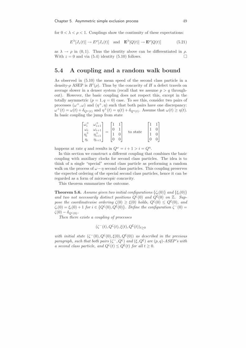
As observed in (5.10) the mean speed of the second class particle in adensity-ρ ASEP is H ′(ρ). Thus by the concavity of H a defect travels onaverage slower in a denser system (recall that we assume p > q through-out). However, the basic coupling does not respect this, except in thetotally asymmetric (p = 1, q = 0) case. To see this, consider two pairs ofprocesses (ω+, ω) and (η+, η) such that both pairs have one discrepancy:ω+(t) = ω(t) + δQω(t) and η+(t) = η(t) + δQη(t). Assume that ω(t) ≥ η(t).In basic coupling the jump from state
ω+i ω+
i+1
ωi ωi+1
η+i η+
i+1
ηi ηi+1
=
1 10 11 00 0
to state
1 11 01 00 0
happens at rate q and results in Qω = i + 1 > i = Qη.In this section we construct a different coupling that combines the basic
coupling with auxiliary clocks for second class particles. The idea is tothink of a single “special” second class particle as performing a randomwalk on the process of ω−η second class particles. This coupling preservesthe expected ordering of the special second class particles, hence it can beregarded as a form of microscopic concavity.
This theorem summarizes the outcome.
Theorem 5.6. Assume given two initial configurations ζi(0) and ξi(0)and two not necessarily distinct positions Qζ(0) and Qξ(0) on Z. Sup-pose the coordinatewise ordering ζ(0) ≥ ξ(0) holds, Qζ(0) ≤ Qξ(0), andζi(0) = ξi(0) + 1 for i ∈ Qζ(0), Qξ(0). Define the configuration ζ−(0) =ζ(0) − δQζ(0).
Then there exists a coupling of processes
(ζ−(t), Qζ(t), ξ(t), Qξ(t))t≥0
with initial state (ζ−(0), Qζ(0), ξ(0), Qξ(0)) as described in the previousparagraph, such that both pairs (ζ−, Qζ) and (ξ,Qξ) are (p, q)-ASEP’s witha second class particle, and Qζ(t) ≤ Qξ(t) for all t ≥ 0.
50 Timo Seppalainen
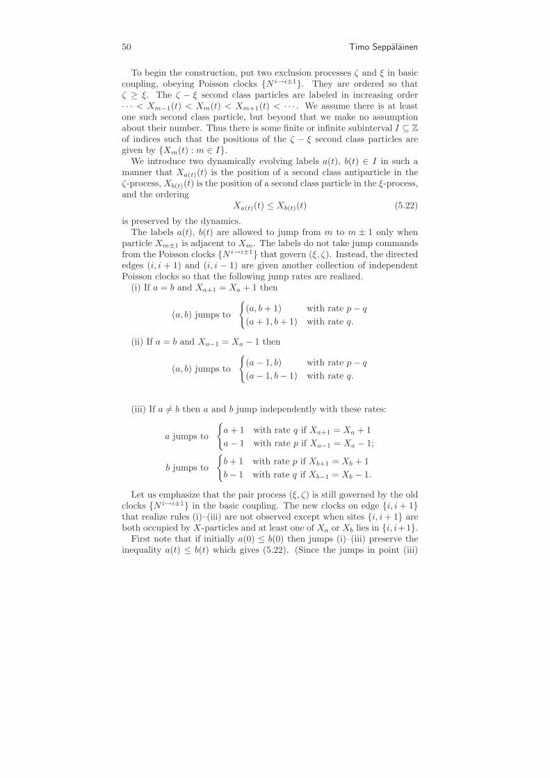
To begin the construction, put two exclusion processes ζ and ξ in basiccoupling, obeying Poisson clocks N i→i±1. They are ordered so thatζ ≥ ξ. The ζ − ξ second class particles are labeled in increasing order· · · < Xm−1(t) < Xm(t) < Xm+1(t) < · · · . We assume there is at leastone such second class particle, but beyond that we make no assumptionabout their number. Thus there is some finite or infinite subinterval I ⊆ Z
of indices such that the positions of the ζ − ξ second class particles aregiven by Xm(t) : m ∈ I.
We introduce two dynamically evolving labels a(t), b(t) ∈ I in such amanner that Xa(t)(t) is the position of a second class antiparticle in theζ-process, Xb(t)(t) is the position of a second class particle in the ξ-process,and the ordering
Xa(t)(t) ≤ Xb(t)(t) (5.22)
is preserved by the dynamics.The labels a(t), b(t) are allowed to jump from m to m ± 1 only when
particle Xm±1 is adjacent to Xm. The labels do not take jump commandsfrom the Poisson clocks N i→i±1 that govern (ξ, ζ). Instead, the directededges (i, i + 1) and (i, i − 1) are given another collection of independentPoisson clocks so that the following jump rates are realized.
(i) If a = b and Xa+1 = Xa + 1 then
(a, b) jumps to
(a, b + 1) with rate p − q
(a + 1, b + 1) with rate q.
(ii) If a = b and Xa−1 = Xa − 1 then
(a, b) jumps to
(a − 1, b) with rate p − q
(a − 1, b − 1) with rate q.
(iii) If a 6= b then a and b jump independently with these rates:
a jumps to
a + 1 with rate q if Xa+1 = Xa + 1
a − 1 with rate p if Xa−1 = Xa − 1;
b jumps to
b + 1 with rate p if Xb+1 = Xb + 1
b − 1 with rate q if Xb−1 = Xb − 1.
Let us emphasize that the pair process (ξ, ζ) is still governed by the oldclocks N i→i±1 in the basic coupling. The new clocks on edge i, i + 1that realize rules (i)–(iii) are not observed except when sites i, i + 1 areboth occupied by X-particles and at least one of Xa or Xb lies in i, i+1.
First note that if initially a(0) ≤ b(0) then jumps (i)–(iii) preserve theinequality a(t) ≤ b(t) which gives (5.22). (Since the jumps in point (iii)
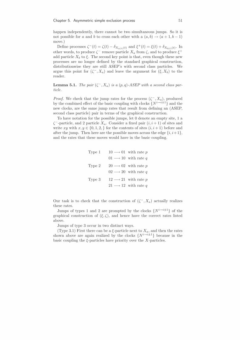
Chapter 5. Asymmetric simple exclusion process 51
happen independently, there cannot be two simultaneous jumps. So it isnot possible for a and b to cross each other with a (a, b) → (a + 1, b − 1)move.)
Define processes ζ−(t) = ζ(t) − δXa(t)(t) and ξ+(t) = ξ(t) + δXb(t)(t). In
other words, to produce ζ− remove particle Xa from ζ, and to produce ξ+
add particle Xb to ξ. The second key point is that, even though these newprocesses are no longer defined by the standard graphical construction,distributionwise they are still ASEP’s with second class particles. Weargue this point for (ζ−,Xa) and leave the argument for (ξ,Xb) to thereader.
Lemma 5.1. The pair (ζ−,Xa) is a (p, q)-ASEP with a second class par-ticle.
Proof. We check that the jump rates for the process (ζ−,Xa), producedby the combined effect of the basic coupling with clocks N i→i±1 and thenew clocks, are the same jump rates that result from defining an (ASEP,second class particle) pair in terms of the graphical construction.
To have notation for the possible jumps, let 0 denote an empty site, 1 aζ−-particle, and 2 particle Xa. Consider a fixed pair (i, i + 1) of sites andwrite xy with x, y ∈ 0, 1, 2, for the contents of sites (i, i + 1) before andafter the jump. Then here are the possible moves across the edge i, i+1,and the rates that these moves would have in the basic coupling.
Type 1 10 −→ 01 with rate p
01 −→ 10 with rate q
Type 2 20 −→ 02 with rate p
02 −→ 20 with rate q
Type 3 12 −→ 21 with rate p
21 −→ 12 with rate q
Our task is to check that the construction of (ζ−,Xa) actually realizesthese rates.
Jumps of types 1 and 2 are prompted by the clocks N i→i±1 of thegraphical construction of (ξ, ζ), and hence have the correct rates listedabove.
Jumps of type 3 occur in two distinct ways.
(Type 3.1) First there can be a ξ-particle next to Xa, and then the ratesshown above are again realized by the clocks N i→i±1 because in thebasic coupling the ξ-particles have priority over the X-particles.
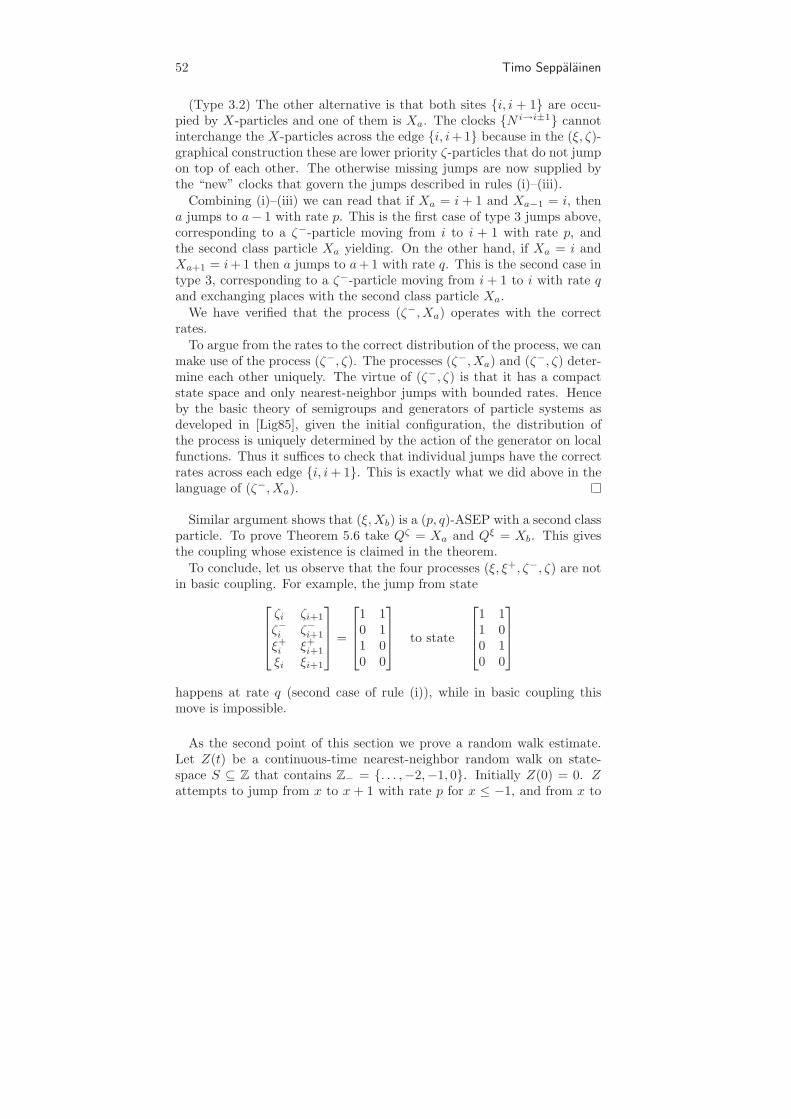
52 Timo Seppalainen
(Type 3.2) The other alternative is that both sites i, i + 1 are occu-pied by X-particles and one of them is Xa. The clocks N i→i±1 cannotinterchange the X-particles across the edge i, i+1 because in the (ξ, ζ)-graphical construction these are lower priority ζ-particles that do not jumpon top of each other. The otherwise missing jumps are now supplied bythe “new” clocks that govern the jumps described in rules (i)–(iii).
Combining (i)–(iii) we can read that if Xa = i + 1 and Xa−1 = i, thena jumps to a− 1 with rate p. This is the first case of type 3 jumps above,corresponding to a ζ−-particle moving from i to i + 1 with rate p, andthe second class particle Xa yielding. On the other hand, if Xa = i andXa+1 = i + 1 then a jumps to a + 1 with rate q. This is the second case intype 3, corresponding to a ζ−-particle moving from i + 1 to i with rate qand exchanging places with the second class particle Xa.
We have verified that the process (ζ−,Xa) operates with the correctrates.
To argue from the rates to the correct distribution of the process, we canmake use of the process (ζ−, ζ). The processes (ζ−,Xa) and (ζ−, ζ) deter-mine each other uniquely. The virtue of (ζ−, ζ) is that it has a compactstate space and only nearest-neighbor jumps with bounded rates. Henceby the basic theory of semigroups and generators of particle systems asdeveloped in [Lig85], given the initial configuration, the distribution ofthe process is uniquely determined by the action of the generator on localfunctions. Thus it suffices to check that individual jumps have the correctrates across each edge i, i + 1. This is exactly what we did above in thelanguage of (ζ−,Xa).
Similar argument shows that (ξ,Xb) is a (p, q)-ASEP with a second classparticle. To prove Theorem 5.6 take Qζ = Xa and Qξ = Xb. This givesthe coupling whose existence is claimed in the theorem.
To conclude, let us observe that the four processes (ξ, ξ+, ζ−, ζ) are notin basic coupling. For example, the jump from state
ζi ζi+1
ζ−i ζ−i+1
ξ+i ξ+
i+1
ξi ξi+1
=
1 10 11 00 0
to state
1 11 00 10 0
happens at rate q (second case of rule (i)), while in basic coupling thismove is impossible.
As the second point of this section we prove a random walk estimate.Let Z(t) be a continuous-time nearest-neighbor random walk on state-space S ⊆ Z that contains Z− = . . . ,−2,−1, 0. Initially Z(0) = 0. Zattempts to jump from x to x + 1 with rate p for x ≤ −1, and from x to
Chapter 5. Asymmetric simple exclusion process 53
x − 1 with rate q for x ≤ 0. Assume p > q = 1 − p and let θ = p − q. Therates on S r Z− need not be specified.
Whether jumps are permitted or not is determined by a fixed environ-ment expressed in terms of 0, 1-valued functions u(x, t) : x ∈ S, 0 ≤t < ∞. A jump across edge x − 1, x in either direction is permitted attime t if u(x, t) = 1, otherwise not. In other words, u(x, t) is the indicatorof the event that edge x − 1, x is open at time t.
Assumption. Assume that for all x ∈ S and T < ∞, u(x, t) flipsbetween 0 and 1 only finitely many times during 0 ≤ t ≤ T . Assume forconvenience right-continuity: u(x, t+) = u(x, t).
Lemma 5.2. For all t ≥ 0 and k ≥ 0,
PZ(t) ≤ −k ≤ e−2θk.
This bound holds for any fixed environment u(x, t) subject to the as-sumption above.
Proof. Let Y (t) be a walk that operates exactly as Z(t) on Z− but isrestricted to remain in Z− by setting the rate of jumping from 0 to 1 tozero. Give Y (t) geometric initial distribution
PY (0) = −j = π(j) ≡(1 − q
p
)(q
p
)j
for j ≥ 0.
The initial points satisfy Y (0) ≤ Z(0) a.s. Couple the walks throughPoisson clocks so that the inequality Y (t) ≤ Z(t) is preserved for all time0 ≤ t < ∞.
Without the inhomogeneous environment Y (t) would be a stationary,reversible birth and death process. We argue that even with the environ-ment the time marginals Y (t) still have distribution π. This suffices forthe conclusion, for then
PZ(t) ≤ −k ≤ PY (t) ≤ −k = (q/p)k = exp(k log 1−θ
1+θ
)≤ e−2θk.
To justify the claim about Y (t), consider approximating processesY (m)(t), m ∈ N, with the same initial value Y (m)(0) = Y (0). Y (m)(t)evolves so that the environments u(x, t) restrict its motion only on edgesx − 1, x for −m + 1 ≤ x ≤ 0. In other words, for walk Y (m)(t) we setu(x, t) ≡ 1 for x ≤ −m and 0 ≤ t < ∞. We couple the walks together sothat Y (t) = Y (m)(t) until the first time one of the walks exits the interval−m + 1, . . . , 0.
Fixing m for a moment, let 0 = s0 < s1 < s2 < s3 < . . . be a partitionof the time axis so that sj ր ∞ and the environments u(x, t) : −m <x ≤ 0 are constant on each interval t ∈ [si, si+1). Then on each time
54 Timo Seppalainen
interval [si, si+1) Y (m)(t) is a continuous time Markov chain with time-homogeneous jump rates
c(x, x + 1) =
pu(x + 1, si), −m ≤ x ≤ 0
p, x ≤ −m − 1
and
c(x, x − 1) =
qu(x, si), −m + 1 ≤ x ≤ 0
q, x ≤ −m.
One can check that detailed balance π(x)c(x, x + 1) = π(x + 1)c(x + 1, x)holds for all x ≤ −1. Thus π is a reversible measure for walk Y (m)(t) oneach time interval [si, si+1), and we conclude that Y (m)(t) has distributionπ for all 0 ≤ t < ∞.
The coupling ensures that Y (m)(t) → Y (t) almost surely as m → ∞,and consequently also Y (t) has distribution π for all 0 ≤ t < ∞.
5.5 Proof of the upper bound for second class
particle moments
AbbreviateΨ(t) = Eρ|Q(t) − V ρt|. (5.23)
Lemma 5.3. Let B ∈ (0,∞). Then there exists a numerical constantC ∈ (0,∞) and another constant c1(B) ∈ (0,∞) such that, for all densities0 < ρ < 1, u ≥ 1, 0 < θ < 1/2, and t ≥ c1(B)θ−1,
PρQ(t) ≥ V ρt + u
≤
Cθ2( t2
u4Ψ(t) +
t2
u3
)+ e−u2/Ct, Bθ2/3t2/3 ≤ u ≤ 20t/3
e−u/C , u ≥ 20t/3.
(5.24)
Proof. First we get an easy case out of the way.
Case 1. u ≥ 5ρθt.
This comes from an exponential Chebyshev argument. Let Zt be anearest-neighbor random walk with rates p = (1 + θ)/2 to the right andq = (1 − θ)/2 to the left. For α ∈ (0, 1], using
eα + e−α
2≤ 1 + α2 and
eα − e−α
2≤ α + α2,
Chapter 5. Asymmetric simple exclusion process 55
we get
E[eαZt ] = exp(−t + t
eα + e−α
2+ θt
eα − e−α
2
)
≤ exp(2α2t + αθt
).
(5.25)
We have the stochastic domination Zt ≥ Q(t) because no matter what theenvironment next to Q(t) is, Q(t) has a weaker right drift than Zt. Then,since V ρ = θ(1 − 2ρ) and 2ρθt ≤ 2u/5,
PρQ(t) ≥ V ρt + u ≤ PZt ≥ θt + 35u
≤ exp(− 3
5αu + 2α2t)
≤
exp(− 9u2
200t ) u ≤ 20t/3
exp(−3u/10) u > 20t/3.
(5.26)
In the last inequality above choose α = 1 ∧ 3u20t . Note that 20t/3 > 5ρθt.
It remains to consider this range of u:
Case 2. Bθ2/3t2/3 ≤ u ≤ 5ρθt.
By an adjustment of the constant C we can assume that u is a positiveinteger. Fix a density 0 < ρ < 1 and an auxiliary density
λ = ρ − u
10θt. (5.27)
Start with the basic coupling of three exclusion processes ω ≥ ω− ≥ ηwith this initial set-up:
(a) Initially ωi(0) : i 6= 0 are i.i.d. Bernoulli(ρ) distributed and ω0(0) =1.
(b) Initially ω−(0) = ω(0) − δ0.(c) Initially variables ηi(0) : i 6= 0 are i.i.d. Bernoulli(λ) and η0(0) = 0.
The coupling of the initial occupations is such that ωi(0) ≥ ηi(0) for alli 6= 0.
Recall that basic coupling meant that these processes obey commonPoisson clocks.
Let Q(t) be the position of the single second class particle between ω(t)and ω−(t), initially at the origin. Let Xi(t) : i ∈ Z be the positions ofthe ω − η second class particles, initially labeled so that
· · · < X−2(0) < X−1(0) < X0(0) = 0 < X1(0) < X2(0) < · · ·
These second class particles preserve their labels in the dynamics andstay ordered. Thus the ω(t) configuration consists of first class particles(the η(t) process) and second class particles (the Xj(t)’s). P denotes theprobability measure under which all these coupled processes live. Note
56 Timo Seppalainen
that the marginal distribution of (ω, ω−, Q) under P is exactly as it wouldbe under Pρ.
For x ∈ Z, Jωx (t) is the net current in the ω-process between space-
time positions (1/2, 0) and (x + 1/2, t). Similarly Jηx (t) in the η-process,
and Jω−ηx (t) is the net current of second class particles. Current in the
ω-process is a sum of the first class particle current and the second classparticle current:
Jωx (t) = Jη
x (t) + Jω−ηx (t). (5.28)
Q(t) ∈ Xj(t) for all time because the basic coupling preserves theordering ω−(t) ≥ η(t). Define the label mQ(t) by Q(t) = XmQ(t)(t) withinitial value mQ(0) = 0.
Lemma 5.4. For all t ≥ 0 and k ≥ 0,
PmQ(t) ≥ k ≤ e−2θk.
Proof of Lemma 5.4. In the basic coupling the label mQ(t) evolves as fol-lows. When XmQ−1 is adjacent to XmQ
, mQ jumps down by one at ratep. And when XmQ+1 is adjacent to XmQ
, mQ jumps up by one at rateq. When XmQ
has no X-particle in either neighboring site, the label mQ
cannot jump. Thus the situation is like that in Lemma 5.2 (with a re-versal of lattice directions) with environment given by the adjacency ofX-particles: u(m, t) = 1Xm(t) = Xm−1(t) + 1. However, the basic cou-pling mixes together the evolution of the environment and the walk mQ,so the environment is not specified in advance as required by Lemma 5.2.
We can get around this difficulty by imagining an alternative but dis-tributionally equivalent construction for the joint process (η, ω−, ω). Let(η, ω) obey basic coupling with the given Poisson clocks Nx→x±1 at-tached to directed edges (x, x± 1). Divide the ω − η particles further intoclass II consisting of the particles ω− − η and class III that consists onlyof the single particle ω − ω− = δQ. Let class II have priority over class
III. Introduce another independent set of Poisson clocks Nx→x±1, alsoattached to directed edges (x, x ± 1) of the space Z where particles move.
Let clocks Nx→x±1 govern the exchanges between classes II and III. In
other words, for each edge x, x + 1 clocks Nx→x+1 and Nx+1→x are ob-served if sites x, x + 1 are both occupied by ω − η particles. All otherjumps are prompted by the original clocks.
The rates for individual jumps are the same in this alternative con-struction as in the earlier one where all processes were together in basiccoupling. Thus the same distribution for the process (η, ω−, ω) is created.
To apply Lemma 5.2 perform the construction in two steps. First con-struct the process (η, ω) for all time. This determines the environment
Chapter 5. Asymmetric simple exclusion process 57
u(m, t) = 1Xm(t) = Xm−1(t) + 1. Then run the dynamics of classes IIand III in this environment. Now Lemma 5.2 gives the bound for mQ.
Let u be a positive integer and
k =
⌊u2
20θt
⌋− 3. (5.29)
By assuming t ≥ C(B)θ−1 we guarantee that
u ≥ 1 andu2
40θt≥ B2θ1/3t1/3
40≥ 4.
Then
k ≥ u2
40θt≥ 4. (5.30)
We begin a series of inequalities.
PQ(t) ≥ V ρt + u≤ PmQ(t) ≥ k + PJω
⌊V ρt⌋+u(t) − Jη⌊V ρt⌋+u(t) > −k. (5.31)
To explain the inequality above, if Q(t) ≥ V ρt + u and mQ(t) < k thenXk(t) > ⌊V ρt⌋ + u. This puts the bound
Jω−η⌊V ρt⌋+u(t) > −k
on the second class particle current, because at most particles X1, . . . ,Xk−1
could have made a negative contribution to this current.
Lemma 5.4 takes care of the first probability on line (5.31). We workon the second probability on line (5.31).
Here is a simple observation that will be used repeatedly. Process ω canbe coupled with a stationary density-ρ process ω(ρ) so that the coupledpair (ω, ω(ρ)) has at most 1 discrepancy. In this coupling
|Jωx (t) − Jω(ρ)
x (t)| ≤ 1. (5.32)
This way we can use computations for stationary processes at the expenseof small errors.
Recall that V ρ = H ′(ρ). Let c1 below be a constant that absorbs theerrors from using means of stationary processes and from ignoring integer
58 Timo Seppalainen
parts. It satisfies |c1| ≤ 3.
EJω⌊V ρt⌋+u(t) − EJη
⌊V ρt⌋+u(t) (5.33)
= tH(ρ) − (H ′(ρ)t + u)ρ − tH(λ) + (H ′(ρ)t + u)λ + c1
= − 12 tH ′′(ρ)(ρ − λ)2 − u(ρ − λ) + c1
= tθ(ρ − λ)2 − u(ρ − λ) + c1
= tθ(ρ − λ)2 − u(ρ − λ) + c1 + k − k
≤ u2
100tθ− u2
10tθ+
u2
20tθ− k
= − u2
25tθ− k. (5.34)
The −3 in the definition (5.29) of k absorbed c1 above.
Let X = X − EX denote a centered random variable. Continuing withthe second probability from line (5.31):
PJω⌊V ρt⌋+u(t) − Jη
⌊V ρt⌋+u(t) > −k
≤ P
Jω
⌊V ρt⌋+u(t) − Jη
⌊V ρt⌋+u(t) ≥ u2
25tθ
≤ Cθ2t2
u4Var
Jω⌊V ρt⌋+u(t) − Jη
⌊V ρt⌋+u(t)
≤ Cθ2t2
u4
(Var
Jω⌊V ρt⌋+u(t)
+ Var
Jη⌊V ρt⌋+u(t)
). (5.35)
C is a numerical constant that can change from line to line but is inde-pendent of all the parameters.
We develop bounds on the variances above, first for Jω. Pass to thestationary density-ρ process via (5.32) and apply (5.11):
VarJω⌊V ρt⌋+u(t)
≤ 2Varρ
J⌊V ρt⌋+u(t)
+ 2
= 2ρ(1 − ρ)E∣∣Q(t) − ⌊V ρt⌋ − u
∣∣ + 2
≤ E|Q(t) − V ρt | + u + 3
≤ Ψ(t) + 4u. (5.36)
Let Varλ denote variance in the stationary density-λ process and letQη(t) denote the position of a second class particle added to a process η.
VarJη⌊V ρt⌋+u(t)
≤ 2Varλ
J⌊V ρt⌋+u(t)
+ 2
≤ Eλ∣∣Qη(t) − ⌊V ρt⌋ − u
∣∣ + 2
≤ Eλ|Qη(t) − V ρt | + 4u.
Chapter 5. Asymmetric simple exclusion process 59
Introduce process (ζ−(t), Qζ(t), η(t), Qη(t))t≥0 coupled as in Theorem 5.6,where ζ starts with Bernoulli(ρ) occupations away from the origin andinitially Qζ(0) = Qη(0) = 0. Below apply the triangle inequality and useinequality Qζ(t) ≤ Qη(t) from Theorem 5.6. Thus continuing from above:
= E|Qη(t) − Qζ(t) + Qζ(t) − V ρt | + 4u
≤ EQη(t) − Qζ(t)
+ E|Qζ(t) − V ρt | + 4u
= V λt − V ρt + Ψ(t) + 4u
= 2θt(ρ − λ) + Ψ(t) + 4u
= Ψ(t) + 5u. (5.37)
Marginally the process (ζ,Qζ) is the same as the process (ω,Q) in thecoupling of this section, hence the appearance of Ψ(t) above. Then weused (5.10) for the expectations of the second class particles and the choice(5.27) of λ.
Insert bounds (5.36) and (5.37) into (5.35) to get
PJω⌊V ρt⌋+u(t) − Jη
⌊V ρt⌋+u(t) > −k ≤ Cθ2( t2
u4Ψ(t) +
t2
u3
). (5.38)
Insert (5.30) and (5.38) into line (5.31) to get
PQ(t) ≤ V ρt − u ≤ Cθ2( t2
u4Ψ(t) +
t2
u3
)+ e−u2/20t (5.39)
and we have verified (5.24) for Case 2.
Combining (5.39) and (5.26) gives the conclusion of Lemma 5.3.
Next we extend the bound to both tails.
Lemma 5.5. Let B ∈ (0,∞). Then there exists a numerical constantC ∈ (0,∞) and another constant c0(B) ∈ (0,∞) such that, for all densities0 < ρ < 1 and t ≥ c0(B)θ−1,
Pρ |Q(t) − V ρt| ≥ u
≤
Cθ2( t2
u4Ψ(t) +
t2
u3
)+ 2e−u2/Ct, Bθ2/3t2/3 ≤ u ≤ 20t/3
2e−u/C , u ≥ 20t/3.
(5.40)
Proof. The corresponding lower tail bound is obtained from (5.24) by aparticle-hole interchange followed by a reflection of the lattice. For detailswe refer to Lemma 5.3 in [BS09a].
60 Timo Seppalainen
Proof of the upper bound of Theorem 5.4. We integrate (5.40) to get thebound (5.13) on the moments of the second class particle. First for m = 1.
Ψ(t) =
∫ ∞
0
Pρ |Q(t) − V ρt| ≥ u du
≤ Bθ2/3t2/3 + Cθ2
∫ ∞
Bθ2/3t2/3
( t2
u4Ψ(t) +
t2
u3
)du
+ 2
∫ ∞
Bθ2/3t2/3
e−u2/Ct du + 2
∫ ∞
20t/3
e−u/C du
≤ C
3B3Ψ(t) +
(B +
C
2B2
)θ2/3t2/3
+C1(B)t1/3
θ2/3e−θ4/3t1/3/C1(B) + 2Ce−t/C .
C1(B) is a new constant that depends on B. Set B = C1/3 to turn theabove inequality into
Ψ(t) ≤ 9C1/3
4θ2/3t2/3 +
C1t1/3
θ2/3exp
(−θ4/3t1/3
C1
)+ 2Ce−t/C .
The second term on the right above forces us to restrict t further. We canfix a constant c0 large enough so that, for a new constant C,
Ψ(t) ≤ Cθ2/3t2/3 provided t ≥ c0θ−4. (5.41)
Restrict to t that satisfy this requirement and substitute this bound onΨ(t) into (5.40). Then upon using u ≥ Bθ2/3t2/3 and redefining C oncemore, we have for Bθ2/3t2/3 ≤ u ≤ 20t/3:
Pρ |Q(t) − V ρt| ≥ u ≤ Cθ2t2
u3+ 2e−u2/Ct. (5.42)
Now take 1 < m < 3 and use (5.42) together with the second case of(5.40):
Eρ|Q(t) − V ρt|m = m
∫ ∞
0
Pρ |Q(t) − V ρt| ≥ uum−1 du
≤ Bmθ2m/3t2m/3 + Cmθ2t2∫ ∞
Bθ2/3t2/3
um−4 du
+ 2m
∫ ∞
Bθ2/3t2/3
e−u2/Ctum−1 du + 2m
∫ ∞
20t/3
e−u/Cum−1 du.
Performing and approximating the integrals gives
Eρ|Q(t) − V ρt|m ≤ C
3 − mθ2m/3t2m/3
provided t ≥ c0θ−4 for a large enough constant c0.
Chapter 5. Asymmetric simple exclusion process 61
5.6 Proof of the lower bound for second class
particle moments
By Jensen’s inequality it suffices to prove the lower bound for m = 1.Let CUB denote the constant in the upper bound statement that we justproved. We can also assume c0 ≥ 1. Fix a constant b > 0 and set
a1 = 2CUB + 1 and a2 = 8 +√
32b + 8√
CUB .
Increase b if necessary so that
b2 − 2a2 ≥ 1. (5.43)
Fix a density ρ ∈ (0, 1) and define an auxiliary density λ = ρ−bt−1/3θ−1/3.Define positive integers
u = ⌊a1t2/3θ2/3⌋ and n = ⌊V λt⌋ − ⌊V ρt⌋ + u. (5.44)
By taking c0 large enough in the statement of Theorem 5.4 we can ensurethat λ ∈ (ρ/2, ρ) and u ∈ N.
Construct a basic coupling of three processes η ≤ η+ ≤ ζ with thefollowing initial state:
(a) Initially η has i.i.d. Bernoulli(λ) occupations ηi(0) : i 6= −n andη−n(0) = 0.
(b) Initially η+(0) = η(0) + δ−n. Q(−n)(t) is the location of the uniquediscrepancy between η(t) and η+(t).
(c) Initially ζ has independent occupation variables, coupled with η(0)as follows:
(c.1) ζi(0) = ηi(0) for −n < i ≤ 0.(c.2) ζ−n(0) = 1.(c.3) For i < −n and i > 0 variables ζi(0) are i.i.d. Bernoulli(ρ) and
ζi(0) ≥ ηi(0).Thus the initial density of ζ is piecewise constant: on the segment −n+
1, . . . , 0 ζ(0) is i.i.d. with density λ, at site −n ζ(0) has density 1, andelsewhere on Z ζ(0) is i.i.d. with density ρ. The reason for the gap inthe ζ − η second class particles across (−n, 0] is to get an upper boundon the second-class particle current that is not too large for subsequentarguments ((5.48) below).
Label the ζ−η second class particles as Ym(t) : m ∈ Z so that initially
· · · < Y−1(0) < Y0(0) = −n = Q(−n)(0) < 0 < Y1(0) < Y2(0) < · · ·
Let again mQ(t) be the label such that Q(−n)(t) = YmQ(t)(t). Initially
mQ(0) = 0. The inclusion Q(−n)(t) ∈ Ym(t) persists for all time because
62 Timo Seppalainen
the basic coupling preserves the ordering ζ(t) ≥ η+(t). Through the basiccoupling mQ jumps to the left with rate q and to the right with rate p,but only when there is a Y -particle adjacent to YmQ
. As in the proof ofLemma 5.4 we can apply Lemma 5.2 to prove this statement:
PmQ(t) ≤ −k ≤ e−2θk. (5.45)
By the upper bound already proved and by the choice of a1,
PQ(−n)(t) ≥ ⌊V ρt⌋ = PQ(−n)(t) ≥ −n + ⌊V λt⌋ + u
≤ u−1E|Q(−n)(t) − n − ⌊V λt⌋| ≤ CUBt2/3θ2/3
⌊a1t2/3θ2/3⌋≤ 1
2 .
(5.46)
For the complementary event we get a lower bound:
12 ≤ PQ(−n)(t) ≤ ⌊V ρt⌋≤ Pm(t) ≤ −k + PJζ
⌊V ρt⌋(t) − Jη⌊V ρt⌋(t) ≤ k.
(5.47)
The reasoning behind the second inequality above is this. If Q(−n)(t) ≤⌊V ρt⌋ and mQ(t) > −k then Y−k(t) ≤ ⌊V ρt⌋. This implies a bound on thesecond class particle current:
Jζ⌊V ρt⌋(t) − Jη
⌊V ρt⌋(t) = Jζ−η⌊V ρt⌋(t) ≤ k. (5.48)
Put k = ⌊a2t1/3θ1/3⌋ − 2. Then by t ≥ θ−4 and the definition of a2,
PmQ(t) ≤ −k ≤ e−2 < 1/4. (5.49)
Combine (5.47) and (5.49) and split the probability:
14 ≤ PJζ
⌊V ρt⌋(t) − Jη⌊V ρt⌋(t) ≤ a2t
1/3θ1/3 − 2≤ PJζ
⌊V ρt⌋(t) ≤ 2a2t1/3θ1/3 + tθ(2ρλ − λ2)
+ PJη⌊V ρt⌋(t) ≥ a2t
1/3θ1/3 + tθ(2ρλ − λ2) + 2. (5.50)
Consider next line (5.50). The η-process can be coupled with a station-ary Pλ-process with at most one discrepancy. The mean current in thestationary process is
Eλ[J⌊V ρt⌋(t)] = tH(λ) − λ⌊V ρt⌋≤ tH(λ) − λV ρt + 1 = tθ(2ρλ − λ2) + 1.
Chapter 5. Asymmetric simple exclusion process 63
Hence
line (5.50) ≤ PλJ⌊V ρt⌋(t) ≥ a2t1/3θ1/3 + tθ(2ρλ − λ2) + 1
≤ PλJ⌊V ρt⌋(t) ≥ a2t
1/3θ1/3≤ a−2
2 t−2/3θ−2/3 Varλ[J⌊V ρt⌋(t)
]
≤ Eλ|Q(t) − ⌊V ρt⌋|a22t
2/3θ2/3≤ Eλ|Q(t) − V λt|
a22t
2/3θ2/3+
2b
a22
+1
a22t
2/3θ2/3
≤ CUBa−22 + 1
16 + 164 ≤ 1
8 . (5.51)
After Chebyshev above we applied the basic identity (5.11) for which weintroduced a second class particle Q(t) in a density-λ system under themeasure Pλ. Then we replaced ⌊V ρt⌋ with V λt and applied the upperbound and properties of a2.
Put this last bound back into line (5.50) to be left with
18 ≤ PJζ
⌊V ρt⌋(t) ≤ 2a2t1/3θ1/3 + tθ(2ρλ − λ2). (5.52)
Next we replace the ζ-process with a stationary density-ρ process byinserting the Radon-Nikodym factor. Let γ denote the distribution ofthe initial ζ(0) configuration described by (c1)–(c3) in the beginning ofthis section. As before νρ is the density-ρ i.i.d. Bernoulli measure. TheRadon-Nikodym derivative is
f(ω) =dγ
dνρ(ω) =
1
ρ1ω−n = 1 ·
0∏
i=−n+1
(λ
ρ1ωi = 1+
1 − λ
1 − ρ1ωi = 0
).
Bound its second moment:
Eρ(f2) =1
ρ
(1 +
(ρ − λ)2
ρ(1 − ρ)
)n
≤ ρ−1en(ρ−λ)2/ρ(1−ρ) ≤ c2(ρ) (5.53)
where condition t ≥ c0θ−4 implies a bound c2(ρ) < ∞ independent of t
and θ.Let A denote the exclusion process event
A = J⌊V ρt⌋(t) ≤ 2a2t1/3θ1/3 + tθ(2ρλ − λ2).
Then from (5.52)
18 ≤ Pζ ∈ A =
∫Pω(A) γ(dω) =
∫Pω(A)f(ω) νρ(dω)
≤(P ρ(A)
)1/2(Eρ(f2)
)1/2 ≤ c2(ρ)1/2(P ρ(A)
)1/2. (5.54)
Note the stationary mean
Eρ[J⌊V ρt⌋(t)
]= tH(ρ) − ρ⌊V ρt⌋ = tθρ2 + ρV ρt − ρ⌊V ρt⌋ ≥ tθρ2.
64 Timo Seppalainen
Continue from line (5.54), recalling (5.43):
(64c2(ρ))−1 ≤ P ρ(A) = P ρJ⌊V ρt⌋(t) ≤ 2a2t1/3θ1/3 + tθ(2ρλ − λ2)
≤ P ρJ⌊V ρt⌋(t) ≤ 2a2t1/3θ1/3 − tθ(ρ − λ)2
= P ρJ⌊V ρt⌋(t) ≤ −(b2 − 2a2)t1/3θ1/3
≤ P ρJ⌊V ρt⌋(t) ≤ −t1/3θ1/3≤ t−2/3θ−2/3 Varρ
[J⌊V ρt⌋(t)
]≤ t−2/3θ−2/3Eρ|Q(t) − V ρt|.
This completes the proof of the lower bound. We finish with someobservations about the need for the two key assumptions, asymmetry andH ′′(ρ) 6= 0.
For symmetric SEP θ = 0 and consequently the Chebyshev step abovecannot be taken.
To observe where H ′′(ρ) < 0 came in we need to backtrack a little.At stage (5.52) we have the inequality (ignoring now small errors due tointeger parts etc.)
18 ≤ P
Jζ⌊V ρt⌋(t) ≤ 2a2t
1/3θ1/3 + Eλ(J⌊V ρt⌋(t)).
The Radon-Nikodym and Schwarz trick turned this into an inequality fora stationary process:
0 < c ≤ P ρJ⌊V ρt⌋(t) ≤ 2a2t
1/3θ1/3 + Eλ(J⌊V ρt⌋(t))
= P ρJ⌊V ρt⌋(t) ≤ 2a2t
1/3θ1/3 + Eλ(J⌊V ρt⌋(t)) − Eρ(J⌊V ρt⌋(t)).
(5.55)
Compute the means on the right-hand side inside the probability, remem-bering that V ρ = H ′(ρ) and Taylor expanding H(λ):
Eλ(J⌊V ρt⌋(t)) − Eρ(J⌊V ρt⌋(t)) = t[H(λ) − λH ′(ρ) − H(ρ) + ρH ′(ρ)
]
= t[12H ′′(ρ)(λ − ρ)2 + O
(θ|λ − ρ|3
)]
= −a3b2t1/3θ1/3 + O(1)
with 12H ′′(ρ) = −a3θ < 0 in the last step. Thus the constants can be
adjusted so that the probability in (5.55) is a deviation. Chebyshev canbe applied to conclude that the current variance is of order t2/3θ2/3. Butif H ′′(ρ) = 0 there is no deviation to take advantage of.
Further comments and references
The proofs of this chapter are based on [BS09a]. This article gives simplerproofs for the results in [BS07] and [BS09b]. Precursors of these vari-ance bounds were first proved for last-passage models that correspond to

Chapter 5. Asymmetric simple exclusion process 65
totally asymmetric versions of particle systems: in [CG06] for the Ham-mersley process and in [BCS06] for the corner growth model associatedwith TASEP.
The Tracy-Widom type limit distribution for TASEP current was firstproved for the step initial condition in [Joh00], then for the stationary case(Theorem 5.5) in [FS06]. The larger picture of TASEP fluctuations fromvarious initial conditions is presented in [BAC09].
Another line of work has produced comparison theorems that allow oneto conclude that Laplace transforms of t−1Varρ[Q(t)] for different asym-metric exclusion processes are within constant multiples of each other. Inthis sense, for the order of this Laplace transform there is universality forall finite range asymmetric exclusion processes. These results come fromresolvent techniques [Set03, QV07, QV08].
The central limit theorem for the current in directions other than thecharacteristic V ρ was proved first by Ferrari and Fontes [FF94]. Thiswas generalized to other particle systems such as certain zero-range andbricklayer processes by Balazs [Bal03].
Consider symmetric simple exclusion, namely the case p = q = 1/2.Then V ρ = 0. Equation (5.11) together with the observation that thesecond class particle is a simple symmetric random walk tell us thatVarρ[J0(t)] is of order t1/2, exactly as for independent particles in Section2. And indeed the current process does converge to fractional Brownianmotion (see [PS08] and its references).
Chapter 6
Zero range process
6.1 Model and results
From the perspective of universality it would be highly desirable to extendthe results of Section 5 beyond exclusion processes. Throughout the 40-year history of the subject of interacting particle systems, the zero range
process has been a much-studied relative of the exclusion process. In thissection we indicate how the bounds for second class particles and currentvariance are proved for a class of totally asymmetric zero range processes(TAZRP) with concave jump rate functions.
Definition and graphical construction. In contrast with the ex-clusion process, the zero range process does not restrict the number ofparticles allowed at a site. The state of the process at time t is η(t) =(ηi(t))i∈Z ∈ Z
Z+ where ηi(t) ∈ Z+ denotes the number of particles present
at site i at time t. We consider the case where particles take only nearest-neighbor jumps to the right.
Each zero range process is characterized by a jump rate function g :Z+ → R+. It automatically has the value g(0) = 0. The meaning of g forthe process is that when the current state is η, g(ηi) is the rate at whichone particle is moved from site i to i + 1. You can interpret this as sayingthat each of the particles at site i jumps independently with rate η−1
i g(ηi)or that some particular one moves next (say, the bottom one is moved tothe top of the next pile) at rate g(ηi). It is immaterial for we do not labelour particles. (Except again we will label certain second class particles aswe did for ASEP, but we will come to that later.) These jump events takeplace independently at all sites, exactly as for ASEP.
We shall assume that
g is nondecreasing and 0 < g(k) ≤ 1 for k > 0. (6.1)
66
Chapter 6. Zero range process 67
With a bounded g we can perform the following concrete constructionof the process η(t) in terms of independent rate 1 Poisson processes Niand i.i.d. Uniform(0, 1) variables Ui,k. Attach clock Ni to site i, and giveeach jump time of Ni its own Ui,k. Now if t is a jump time for Ni with itsuniform Ui,k, then move one particle from i to i + 1 if Ui,k < g(ηi(t−)),otherwise not. Repeat this step at all sites and all jump times. Theresult is the desired one: independently at each site i, a jump from i toi + 1 occurs in the next small time interval (t, t + dt) with probabilityg(ηi(t))dt + O(dt2).
The generator of this TAZRP is
Lϕ(η) =∑
i∈Z
g(ηi)[ϕ(ηi,i+1) − ϕ(η)]
that acts on bounded cylinder functions ϕ on ZZ+ and ηi,i+1 = η − δi +
δi+1. We will not use the generator in the text. It can be used to checkthe invariance of certain distributions on the state space, as for ASEP inRemark 5.2.
Invariant distributions. Part of the reason for the popularity of ZRPis that, just like ASEP, it has i.i.d. invariant distributions. We denotethese by νρ0≤ρ<∞ indexed by density ρ = Eρ(ηi).
Here is the definition of these measures. Let θ denote a real parameter,and on Z+ define a probability distribution
λθ(k) =1
Zθ· eθk
g(k)!,
defined for θ such that
Zθ =∑
k
eθk
g(k)!< ∞.
Here g(0)! = 1 and g(k)! = g(1) · · · g(k) for k > 0. Define the meandensity function ρ(θ) =
∑k kλθ(k). It is smooth and strictly increasing on
the open interval where Zθ < ∞. Let its inverse function be θ(ρ) and thenreparametrize the distributions in terms of density:
νρ0 (k) = λθ(ρ)(k) =
1
Zθ(ρ)· eθ(ρ)k
g(k)!.
Finally, the actual invariant measures for ZRP are the product measureson the state space Z
Z+:
νρ(dη) =⊗
i∈Z
νρ0 (dηi). (6.2)
68 Timo Seppalainen
We write P ρ for probabilities and Eρ for expectations for the stationaryprocess whose marginal η(t) has distribution νρ.
Basic coupling and second class particles. Basic coupling worksexactly as it did for exclusion processes: two (or more) zero range processesobey a common set of Poisson clocks Ni and uniform variables Ui,k.
We write a boldface P for the probability measure when more thanone process are coupled together. In particular, Pρ represents the situa-tion where the initial occupation variables ηi(0) = η+
i (0) are i.i.d. mean-ρBernoulli for i 6= 0, and the second class particle Q starts at Q(0) = 0.
More generally, if two processes η and ω are in basic coupling and ω(0) ≥η(0) (by which we mean coordinatewise ordering ωi(0) ≥ ηi(0) for all i)then the ordering ω(t) ≥ η(t) holds for all 0 ≤ t < ∞. The effect of thebasic coupling is to give priority to the η particles over the ω−η particles.Consequently we can think of the ω-process as consisting of first classparticles (the η particles) and second class particles (the ω − η particles).
Current. The current is defined as for ASEP: for x ∈ Z and t > 0, Jx(t)is the net left-to-right particle current across the straight-line space-timepath from (1/2, 0) to (x + 1/2, t).
The flux function is again
H(ρ) = Eρ[rate of particle flow across a fixed edge] = Eρ[g(ηi)].
Expectations of currents can be computed as for ASEP:
Eρ[Jx(t)] = tH(ρ) − xρ, x ∈ Z, t ≥ 0. (6.3)
The characteristic speed at density ρ is defined the same way as before:
V ρ = H ′(ρ). (6.4)
As for ASEP, the first task is to establish the identities that connectcurrent variance and the second class particle. These identities for ZRPdevelop the same way as for ASEP, except that a new initial distributionfor the coupled process appears. Define a probability distribution νρ
0 onZ+ by
νρ0 (k) =
1
Varρ(η0)
∞∑
m=k+1
(m − ρ)νρ0 (m), k ∈ Z+.
Define a product distribution νρ on the state space ZZ+ that obeys the
marginals νρ0 of the stationary distribution at all sites except at the origin
where the distribution is νρ0 :
νρ(dη) =(⊗
i6=0
νρ0 (dηi)
)⊗ νρ
0 (dη0).
Chapter 6. Zero range process 69
Let Pρ be the probability distribution of a pair (η, η+) that satisfiesη+(t) = η(t) + δQ(t) (so there is one discrepancy), obeys basic coupling,and whose initial distribution is such that η(0) ∼ νρ and η+(0) = η(0)+δ0
(in other words, Q(0) = 0).
Theorem 6.1. For any density 0 < ρ < ∞, z ∈ Z and t > 0 we havethese formulas.
Varρ[Jz(t)] =∑
j∈Z
|j − z|Covρ[ηj(t), η0(0)], (6.5)
Covρ[ηj(t), η0(0)] = Varρ(η0)PρQ(t) = j, (6.6)
andEρ[Q(t)] = V ρt. (6.7)
Equation (6.5) is proved the same way as for ASEP. Equation (6.6) andthe definition of νρ
0 come from a short calculation which we show below inSection 6.2. We omit the proof of (6.7). Formulas (6.5) and (6.6) combineto give the key equation that links current variance with the second classparticle:
Varρ[Jz(t)] = Varρ(η0)Eρ|Q(t) − z|. (6.8)
Next we state the main result which again consists of upper and lowermoment bounds for a second class particle, this time under the measurePρ. We need a significant restriction on the concavity of the jump rate g:
∃ 0 < r < 1 such that g(k + 1) − g(k) ≤ r(g(k) − g(k − 1)). (6.9)
A class of examples satisfying this hypotheses is given by g(k) = 1 −exp(−akb) with a > 0, b ≥ 1. g(k) can also be constant from some k0
onwards.
Theorem 6.2. Fix a density 0 < ρ < ∞ and consider a pair of coupledZRP’s under the measure Pρ. Assume the jump rate function g satisfies(6.1) and (6.9). Then for 1 ≤ m < 3, large enough t ∈ R+ and a constantC,
1
Ct2m/3 ≤ Eρ
[|Q(t) − V ρt|m
]≤ C
3 − mt2m/3. (6.10)
The constants C and how large t needs to be may depend on the densityρ. Combining (6.5) and (6.10) gives the bounds for the variance of thecurrent seen by an observer traveling at the characteristic speed V ρ: forlarge enough t,
C−1t2/3 ≤ Varρ[J⌊V ρt⌋(t)] ≤ Ct2/3.
70 Timo Seppalainen
For the remainder of this chapter we discuss parts of the proof. Once wehave the fundamental identities that tie together moments of the secondclass particle and the variance of the current, the proofs for the upperand lower bounds given for ASEP in Sections 5.5 and 5.6 can be adjustedto work for TAZRP. We will not repeat those derivations. Instead, wefocus on the key ingredients that made the argument work for ASEP, anddiscuss how to provide these ingredients for TAZRP. There are two keypoints that we need in order to repeat the argument for TAZRP:
1. We need a construction that includes a given second class particle asa labeled member of a density of second class particles, and then weneed a tail bound for the label as the one given for ASEP in Lemma5.4 and (5.45).
2. We need a coupling that keeps the second class particle of a systemwith higher density behind the second class particle of a system withlower density. For ASEP this was Theorem 5.6, which was used toobtain (5.37) for the ASEP upper bound.
We turn to these points in Section 6.3 below, after developing the varianceformula.
6.2 Variance identity
Define F (−1) = 0 and
F (k) =∞∑
m=k+1
(m − ρ)νρ0 (m)
νρ0 (k)
=Varρ(η0)
νρ0 (k)
νρ0 (k), k ≥ 0.
Interpret below νρ0 (−1) as 0.
Covρ[ηi(t), η0(0)] = Eρ[ηi(t)(η0(0) − ρ)]
=∑
k≥0
E[ηi(t)|η0(0) = k](k − ρ)νρ0 (k)
=∑
k≥0
E[ηi(t)|η0(0) = k](F (k − 1)νρ
0 (k − 1) − F (k)νρ0 (k)
)
=∑
k≥0
E[ηi(t)|η0(0) = k + 1]F (k)νρ0 (k)
−∑
k≥0
E[ηi(t)|η0(0) = k]F (k)νρ0 (k).
Chapter 6. Zero range process 71
Construct a coupling of η+(t) = η(t) + δQ(t) with the discrepancy initiallyat the origin Q(0) = 0, and so that η(0) has νρ-distribution. Then, due tothe product form of the initial distribution,
E[ηi(t)|η0(0) = k + 1] = E[η+i (t)|η+
0 (0) = k + 1] = E[η+i (t)|η0(0) = k].
Then continuing from above,
Covρ[ηi(t), η0(0)] =∑
k≥0
E[η+i (t)|η0(0) = k]F (k)νρ
0 (k)
−∑
k≥0
E[ηi(t)|η0(0) = k]F (k)νρ0 (k)
=∑
k≥0
E[η+i (t) − ηi(t)|η0(0) = k]F (k)νρ
0 (k)
= E[(η+
i (t) − ηi(t))F (η0(0))]
= E[1Q(t) = iF (η0(0))
]
=∑
k≥0
E[1Q(t) = i|η0(0) = k]F (k)νρ0 (k)
= Varρ(η0)∑
k≥0
E[1Q(t) = i|η0(0) = k]νρ0 (k)
= Varρ(η0)PρQ(t) = i.
This proves (6.6).
6.3 Coupling for the zero range process
Next we describe a coupling of two processes with labeled discrepancies(second class particles) between them, and then two randomly evolvinglabels that achieve simultaneously both goals (1) and (2) mentioned above.This construction works for any TAZRP with concave jump rate functiong. Getting tail bounds for the label processes is the serious bottleneck ofthis proof, and that is where we need the restrictive assumption (6.9).
Let two processes η ≤ ω evolve in basic coupling. This pair (η, ω) to-gether with the labeled and ordered ω − η second class particles· · · ≤ X−2(t) ≤ X−1(t) ≤ X0(t) ≤ X1(t) ≤ X2(t) ≤ · · · form a “back-ground” process on which we define two label processes y(t) and z(t). Theω−η second class particles are kept in order by requiring that, whenever asecond class particle jumps to the right, the X-particle with highest labelis moved.
The label processes will satisfy y(t) ≤ z(t), we will be able to bound y(t)stochastically from above, z(t) stochastically from below, and the following
72 Timo Seppalainen
two pairs of processes will individually be in basic coupling:
(ω−, ω) = (ω − δXy, ω) and (η, η+) = (η, η + δXz
). (6.11)
The definition of the label processes is partly forced on us by the re-quirement that jumps of Xy and Xz must replicate the rates required bythe basic coupling. Additionally, we devise the joint process (y, z) so thatthe order y ≤ z is maintained.
The rule is that after each jump among (ω, η) that in any way affectsthe site where Xy resides, the value of y is refreshed randomly. Let a andb denote the minimal and maximal labels at the site i where Xy residesafter the jump. If Xy resides at a site other than Xz, then y chooses anew value y′ according to these probabilities:
y′ =
a with probabilityg(ωi − 1) − g(ηi)
g(ωi) − g(ηi)
b with probabilityg(ωi) − g(ωi − 1)
g(ωi) − g(ηi).
(6.12)
If g(ωi) − g(ηi) = 0 then y′ = a.Similarly, after a jump in the background process that affects the site
where Xz resides, if Xz and Xy are not together, then z takes the newvalue z′ as follows (with b again the maximal label at the site i = Xz afterthe jump):
z′ =
b − 1 with probabilityg(ωi) − g(ηi + 1)
g(ωi) − g(ηi)
b with probabilityg(ηi + 1) − g(ηi)
g(ωi) − g(ηi).
If g(ωi) − g(ηi) = 0 then z′ = b.Finally, if after the jump Xy = Xz = i, then the labels are refreshed
jointly as follows:
(y′
z′
)=
(a
b − 1
)with probability
g(ωi) − g(ηi + 1)
g(ωi) − g(ηi)
(a
b
)with probability
g(ηi + 1) − g(ηi)
g(ωi) − g(ηi)
− g(ωi) − g(ωi − 1)
g(ωi) − g(ηi)
(b
b
)with probability
g(ωi) − g(ωi − 1)
g(ωi) − g(ηi).
Chapter 6. Zero range process 73
If g(ωi) − g(ηi) = 0 then (y′, z′) = (a, b).The jump rules preserve y ≤ z. Note that marginally y′ obeys proba-
bilities (6.12), and similarly for z′. Concavity of g was used to define themiddle case in the joint rule.
Let us observe why these rules give the pair (ω−, ω) = (ω − δXy, ω) the
same rates this pair would have in basic coupling. The requirement isthat a jump across edge (i, i + 1) occur for both processes at rate g(ω−
i ),and only for ω at rate g(ωi) − g(ω−
i ). This requires thinking through afew cases. Only the site where Xy resides needs attention since elsewhere(ω−, ω) jump together according to ZRP rates.
(i) In the basic coupling of (η, ω), an (i, i + 1) jump occurs in η at rateg(ηi). Then both ω and ω− experience this jump.
(ii) An ω − η second class particle jumps at rate g(ωi) − g(ηi). Prior tothis jump y chose the top label with probability given by the secondline of (6.12), hence the rate at which Xy jumps is
(g(ωi) − g(ηi)
)· g(ωi) − g(ωi − 1)
g(ωi) − g(ηi)= g(ωi) − g(ωi − 1).
Thus at this rate ω experiences the jump but ω− does not.
If prior to this jump y chose the bottom label, then both ω and ω−
experience this jump, and this happens with rate
(g(ωi) − g(ηi)
)· g(ωi − 1) − g(ηi)
g(ωi) − g(ηi)= g(ωi − 1) − g(ηi).
Adding up the rates we see that the rates of basic coupling have beenrealized. A similar argument is given for (η, η+) = (η, η + δXz
).
We come to the unique point in the proof where assumption (6.9) isused, namely the tail bounds for the labels.
Lemma 6.1. Let the labels start with y(0) = z(0) = 0. Under assumption(6.9) we have these bounds: Py(t) ≥ k ≤ rk and Pz(t) ≤ −k ≤ rk forall k ∈ Z+ and t ≥ 0.
Proof. We do the proof for y(t). The bounds are valid conditionally onthe evolution (η, ω) of the background process. So assume this backgroundevolution given. Then we think of y(t) as an integer-valued Markov chainthat is subject to jumps triggered by the background environment. Eachjump happens at some site i with range of labels a, . . . , b and occupationvariables ωi > ηi ≥ 0 that together satisfy
ωi − ηi = b − a + 1.
74 Timo Seppalainen
Given the current value y, the new value y′ is obtained by the followingrules, which of course are consistent with (6.12): if g(ωi) − g(ηi) = 0 then
y′ =
y if y < a or y > b
a if y ∈ a, . . . , b (6.13)
while if g(ωi) − g(ηi) > 0 then
y′ =
y if y < a or y > b
a with probabilityg(ωi − 1) − g(ηi)
g(ωi) − g(ηi)if y ∈ a, . . . , b
b with probabilityg(ωi) − g(ωi − 1)
g(ωi) − g(ηi)if y ∈ a, . . . , b.
(6.14)
There are infinitely many such jumps in any finite time interval, but allbut finitely many leave y unchanged. To get around this difficulty, we canfirst freeze all the Poisson clocks outside space interval [−M,M ], prove thelemma there, and then let M ր ∞. Since rates are bounded, in any givenbounded block of space-time the finite-M process agrees with the infiniteprocess for all large enough M .
To prove the lemma we show that every jump of type (6.13)–(6.14)preserves the geometric tail bound, regardless of the values a, b, ωi, ηi. Sosuppose y is an integer-valued random variable such that
P (y ≥ k) ≤ rk for k ≥ 0,
and define y′ via (6.13)–(6.14). We wish to show that P (y′ ≥ k) ≤ rk fork ≥ 0.
The case (6.13) is clear since there y′ ≤ y. Let us consider the caseg(ωi) − g(ηi) > 0. Since the jump only redistributes the probability massin a, . . . , b to a, b, it suffices to check that
P (y′ ≥ b) ≤ rb (6.15)
in the case b ≥ 0. Using the jump rule (6.14),
P (y′ ≥ b) = P (y′ = b) + P (y′ ≥ b + 1)
=g(ωi) − g(ωi − 1)
g(ωi) − g(ηi)P (a ≤ y ≤ b) + P (y ≥ b + 1).
If g(ωi)− g(ωi − 1) = 0 the conclusion (6.15) follows from the assumptionon y. So we assume g(ωi) − g(ωi − 1) > 0. Then by concavity all the
Chapter 6. Zero range process 75
g-increments between ηi, . . . , ωi are positive. Next write
P (y′ ≥ b) =g(ωi) − g(ωi − 1)
g(ωi) − g(ηi)
b∑
k=a
(1 − r)rk
+g(ωi) − g(ωi − 1)
g(ωi) − g(ηi)
(P (a ≤ y ≤ b) − ra + rb+1
)
+ P (y ≥ b + 1).
(6.16)
For a ≤ k ≤ b
(1 − r)rk = (1 − r)rb · 1
rb−k≤ (1 − r)rb
ωi−1∏
ℓ=ωi−b+k
g(ℓ) − g(ℓ − 1)
g(ℓ + 1) − g(ℓ)
= (1 − r)rb · g(ωi − b + k) − g(ωi − b + k − 1)
g(ωi) − g(ωi − 1).
Adding these up over a ≤ k ≤ b gives
first term on the right in (6.16)
≤ g(ωi) − g(ωi − 1)
g(ωi) − g(ηi)(1 − r)rb
×b∑
k=a
g(ωi − b + k) − g(ωi − b + k − 1)
g(ωi) − g(ωi − 1)
= (1 − r)rb · g(ωi) − g(ωi − b + a − 1)
g(ωi) − g(ηi)= (1 − r)rb = rb − rb+1.
Substitute this bound back up to (6.16) and use P (y ≥ k) ≤ rk twice:
P (y′ ≥ b) ≤ rb + P (y ≥ b + 1) − rb+1
+g(ωi) − g(ωi − 1)
g(ωi) − g(ηi)
(P (a ≤ y ≤ b) − ra + rb+1
)
≤ rb +g(ωi) − g(ωi − 1)
g(ωi) − g(ηi)
(P (y ≥ a) − ra
)
≤ rb.
Thus (6.15) has been checked and thereby the lemma has been proved fory(t).
References
The results for ZRP are proved in [BKS08]. The case of constant jumprate was done earlier in [BK08].

Bibliography
[BAC09] Gerard Ben Arous and Ivan Corwin, Current fluctua-tions for TASEP: a proof of the Prahofer-Spohn conjecture,arXiv:0905.2993 (2009).
[Bal03] Marton Balazs, Growth fluctuations in a class of depositionmodels, Ann. Inst. H. Poincare Probab. Statist. 39 (2003), no. 4,639–685. MR MR1983174 (2005j:60178a)
[BCS06] Marton Balazs, Eric Cator, and Timo Seppalainen, Cube rootfluctuations for the corner growth model associated to the exclu-sion process, Electron. J. Probab. 11 (2006), no. 42, 1094–1132(electronic). MR MR2268539
[BFP] Jinho Baik, Patrik L. Ferrari, and Sandrine Peche, Limitprocess of stationary tasep near the characteristic line,arXiv:0907.0226.
[BG97] Lorenzo Bertini and Giambattista Giacomin, Stochastic Burg-ers and KPZ equations from particle systems, Comm. Math.Phys. 183 (1997), no. 3, 571–607. MR MR1462228 (99e:60212)
[BK08] Marton Balazs and Julia Komjathy, Order of current vari-ance and diffusivity in the rate one totally asymmetric zerorange process, J. Stat. Phys. 133 (2008), no. 1, 59–78. MRMR2438897 (2009h:60157)
[BKS08] Marton Balazs, Julia Komjathy, and Timo Seppalainen, Micro-scopic concavity and fluctuation bounds in a class of depositionprocesses, arXiv:0808.1177 (2008).
[BQS] Marton Balazs, Jeremy Quastel, and Timo Seppalainen, Scalingexponent for the Hopf-Cole solution of KPZ/stochastic Burgers,arXiv:0909.4816.
77
78 Bibliography
[BRAS06] Marton Balazs, Firas Rassoul-Agha, and Timo Seppalainen,The random average process and random walk in a space-timerandom environment in one dimension, Comm. Math. Phys.266 (2006), 499–545.
[BS] Albert-Laszlo Barabasi and H. Eugene Stanley, Fractal conceptsin surface growth. Cambridge University Press, 1995.
[BS07] Marton Balazs and Timo Seppalainen, Exact connections be-tween current fluctuations and the second class particle in aclass of deposition models, J. Statist. Phys. 127 (2007), 431–455.
[BS09a] Marton Balazs and Timo Seppalainen, Fluctuation bounds forthe asymmetric simple exclusion process, ALEA Lat. Am. J.Probab. Math. Stat. 6 (2009), 1–24. MR MR2485877
[BS09b] Marton Balazs and Timo Seppalainen, Order of current vari-ance and diffusivity in the asymmetric simple exclusion process,arXiv:math/0608400, to appear in Ann. of Math.
[BW71] P. J. Bickel and M. J. Wichura, Convergence criteria for mul-tiparameter stochastic processes and some applications, Ann.Math. Statist. 42 (1971), 1656–1670. MR MR0383482 (52#4363)
[CFP] Ivan Corwin, Patrik L. Ferrari, and Sandrine Peche, Limit pro-cesses of non-equilibrium tasep, arXiv:1002.3476.
[CG06] Eric Cator and Piet Groeneboom, Second class particles andcube root asymptotics for Hammersley’s process, Ann. Probab.34 (2006), no. 4, 1273–1295. MR MR2257647 (2008e:60021)
[DGL85] D. Durr, S. Goldstein, and J. Lebowitz, Asymptotics of parti-cle trajectories in infinite one-dimensional systems with colli-sions, Comm. Pure Appl. Math. 38 (1985), no. 5, 573–597. MRMR803248 (87e:60166)
[Dur04] Richard Durrett, Probability: theory and examples, third ed.,Duxbury Advanced Series, Brooks/Cole–Thomson, Belmont,CA, 2004.
[FF94] P. A. Ferrari and L. R. G. Fontes, Current fluctuations for theasymmetric simple exclusion process, Ann. Probab. 22 (1994),no. 2, 820–832. MR 95j:60162
[FF98] , Fluctuations of a surface submitted to a random aver-age process, Electron. J. Probab. 3 (1998), no. 6, 34 pp. (elec-tronic). MR 99e:60214
Bibliography 79
[FMV03] L. R. G. Fontes, D. P. Medeiros, and M. Vachkovskaia, Timefluctuations of the random average process, Stochastic Pro-cess. Appl. 103 (2003), no. 2, 257–276. MR MR1950766(2003k:60255)
[FS06] Patrik L. Ferrari and Herbert Spohn, Scaling limit for the space-time covariance of the stationary totally asymmetric simple ex-clusion process, Comm. Math. Phys. 265 (2006), no. 1, 1–44.MR MR2217295 (2007g:82038a)
[Joh00] Kurt Johansson, Shape fluctuations and random matrices,Comm. Math. Phys. 209 (2000), no. 2, 437–476. MR2001h:60177
[KKS75] H. Kesten, M. V. Kozlov, and F. Spitzer, A limit law for randomwalk in a random environment, Compositio Math. 30 (1975),145–168. MR MR0380998 (52 #1895)
[Kum08] Rohini Kumar, Space-time current process for independent ran-dom walks in one dimension, ALEA Lat. Am. J. Probab. Math.Stat. 4 (2008), 307–336. MR MR2456971
[Lig85] Thomas M. Liggett, Interacting particle systems, Grundlehrender Mathematischen Wissenschaften [Fundamental Principlesof Mathematical Sciences], vol. 276, Springer-Verlag, New York,1985. MR 86e:60089
[Pet08] Jonathon Peterson, Limiting distributions and large deviationsfor random walks in random environments, Ph.D. thesis, Uni-versity of Minnesota, arXiv:0810.0257, 2008.
[PS] Jonathon Peterson and Timo Seppalainen, Current fluctuationsof a system of one-dimensional random walks in random envi-ronment, arXiv:0904.4768, to appear in Ann. Probab.
[PS08] Magda Peligrad and Sunder Sethuraman, On fractional Brown-ian motion limits in one dimensional nearest-neighbor symmet-ric simple exclusion, ALEA Lat. Am. J. Probab. Math. Stat. 4
(2008), 245–255. MR MR2448774
[PZ09] Jonathon Peterson and Ofer Zeitouni, Quenched limits for tran-sient, zero-speed one-dimensional random walk in random en-vironment, Ann. Probab. 37 (2009), no. 1, 143–188.
[QV07] J. Quastel and B. Valko, t1/3 Superdiffusivity of finite-rangeasymmetric exclusion processes on Z, Comm. Math. Phys. 273
(2007), no. 2, 379–394. MR MR2318311
80 Bibliography
[QV08] J. Quastel and B. Valko, A note on the diffusivity of finite-rangeasymmetric exclusion processes on Z, In and out equilibrium 2,Progress in Probability (V. Sidoravicius and M. E. Vares, eds.),vol. 60, Birkhauser, 2008, pp. 543–550.
[RAS05] Firas Rassoul-Agha and Timo Seppalainen, An almost sure in-variance principle for random walks in a space-time randomenvironment, Probab. Theory Related Fields 133 (2005), no. 3,299–314. MR MR2198014
[Sep05] Timo Seppalainen, Second-order fluctuations and currentacross characteristic for a one-dimensional growth model of in-dependent random walks, Ann. Probab. 33 (2005), no. 2, 759–797. MR MR2123209 (2006d:60153)
[Sep08] , Directed random growth models on the plane, Analy-sis and Stochastics of Growth Processes and Interface Models(P. Morters et al., eds.), Oxford University Press, Oxford, UK,2008, pp. 9–38.
[Set03] Sunder Sethuraman, An equivalence of H−1 norms for the sim-ple exclusion process, Ann. Probab. 31 (2003), no. 1, 35–62.MR MR1959785 (2003k:60264)
[Sol75] Fred Solomon, Random walks in a random environment, Ann.Probability 3 (1975), 1–31. MR MR0362503 (50 #14943)
[Spi76] Frank Spitzer, Principles of random walks, second ed., Springer-Verlag, New York, 1976, Graduate Texts in Mathematics, Vol.34. MR MR0388547 (52 #9383)
[TW08a] Craig A. Tracy and Harold Widom, A Fredholm determinantrepresentation in ASEP, J. Stat. Phys. 132 (2008), no. 2, 291–300. MR MR2415104 (2009d:82108)
[TW08b] , Integral formulas for the asymmetric simple exclusionprocess, Comm. Math. Phys. 279 (2008), no. 3, 815–844. MRMR2386729 (2009e:60217)
[TW09a] , Asymptotics in ASEP with step initial condition,Comm. Math. Phys. 290 (2009), no. 1, 129–154. MRMR2520510
[TW09b] , Total current fluctuations in the asymmetric simpleexclusion process, J. Math. Phys. 50 (2009), no. 9, 095204, 4.MR MR2566884
Bibliography 81
[TW10] , Formulas for joint probabilities for the asymmetricsimple exclusion process, arXiv:1003.3431 (2010).
[Wal86] John B. Walsh, An introduction to stochastic partial differentialequations, Ecole d’ete de probabilites de Saint-Flour, XIV—1984, Lecture Notes in Math., vol. 1180, Springer, Berlin, 1986,pp. 265–439. MR MR876085 (88a:60114)
[Zei04] Ofer Zeitouni, Random walks in random environments, LectureNotes in Mathematics, vol. 1837, Springer-Verlag, Berlin, 2004,Lectures from the 31st Summer School on Probability Theoryheld in Saint-Flour, July 8–25, 2001, Edited by Jean Picard.MR MR2071629
Timo SeppalainenMathematics Department, University of Wisconsin-MadisonMadison, Wisconsin 53706, [email protected]://www.math.wisc.edu/∼seppalai