current topics in medicinal chemistry, 2008 0000 1 weka ...weka machine learning for predicting the...

Current Topics in Medicinal Chemistry, 2008, 8, 0000-0000 1

1568-0266/08 $55.00+.00 © 2008 Bentham Science Publishers Ltd.

Weka Machine Learning for Predicting the Phospholipidosis Inducing Potential

Ovidiu Ivanciuc*

Department of Biochemistry and Molecular Biology, University of Texas Medical Branch, 301 University Boulevard,

Galveston, Texas 77555–0857, USA

Abstract: The drug discovery and development process is lengthy and expensive, and bringing a drug to market may take

up to 18 years and may cost up to 2 billion $US. The extensive use of computer-assisted drug design techniques may

considerably increase the chances of finding valuable drug candidates, thus decreasing the drug discovery time and costs.

The most important computational approach is represented by structure-activity relationships that can discriminate

between sets of chemicals that are active/inactive towards a certain biological receptor. An adverse effect of some cationic

amphiphilic drugs is phospholipidosis that manifests as an intracellular accumulation of phospholipids and formation of

concentric lamellar bodies. Here we present structure-activity relationships (SAR) computed with a wide variety of

machine learning algorithms trained to identify drugs that have phospholipidosis inducing potential. All SAR models are

developed with the machine learning software Weka, and include both classical algorithms, such as k-nearest neighbors

and decision trees, as well as recently introduced methods, such as support vector machines and artificial immune

systems. The best predictions are obtained with support vector machines, followed by a perceptron artificial neural

network, logistic regression, and k-nearest neighbors.

Keywords: Machine learning, support vector machines, artificial immune systems, structure-activity relationships, computer-assisted drug design, phospholipidosis.

1. INTRODUCTION

The current trend in drug discovery and development is an increase of the time and costs required to bring a new drug to market, accompanied by a decrease in the number of new chemical entities approved each year. The drug development phases may take up to 18 years [1], with a median period of 5.1 years for clinical trials and 1.2 years for approval [2]. A cost analysis for 68 randomly selected drugs from 10 pharmaceutical companies shows that the average out-of-pocket cost per new drug is $US 403 million (2000 dollars), which increases to $US 802 million after adding the opportunity cost (the cost of pursuing one choice instead of another) [3]. A more detailed evaluation reveals that the cost per new drug depends significantly on the therapy or the developing firm, and varies between $US 500 million and $US 2,000 million [4]. Another significant feature is the high attrition rate of chemical compounds. The drug discovery process starts with millions of compounds tested in high throughput screening, and the drug development process eventually ends with one successful drug on the market. From all compounds that enter the clinical trials, 30% fail due to lack of efficacy, 30% fail in toxicological and safety tests, and only 11% finish the trials [5]. A study considering all 548 new chemical entities approved between 1975 and 1999 found that 16 drugs (2.9%) were withdrawn from the market [6]. Examples of drugs withdrawn from the market due to adverse reactions include troglitazone (Rezulin) in 2000 [7], cerivastatin (Baycol, Lipobay) in 2001 [8], and rofecoxib (Vioxx) in 2004 [9]. However, the rewards of developing a successful drug can be substantial, as indicated

*Address correspondence to this author at the Department of Biochemistry and Molecular Biology, University of Texas Medical Branch, 301 University Boulevard, Galveston, Texas 77555–0857, USA; E-mail: [email protected]

by the top ten 2006 best selling drugs (in $US billions), namely Lipitor with 14.39 (Pfizer, cholesterol), Advair with 6.13 (GlaxoSmithKline, asthma), Plavix with 6.06 (Bristol-Myers Squibb, vascular disease), Nexium with 5.18 (AstraZeneca, acid reflux), Norvasc with 4.87 (Pfizer, hypertension), Remicade with 4.42 (Johnson & Johnson, rheumatoid arthritis), Enbrel with 4.387 (Amgen, rheumatoid arthritis), Zyprexa with 4.36 (Eli Lilly, schizophrenia), Diovan with 4.22 (Novartis, hypertension), and Risperdal with 4.18 (Johnson & Johnson, schizophrenia).

The rapid pace of drug development is apparent from the large number of research and development projects active as of May 2008, with the top five places occupied by GlaxoSmithKline with 243 projects, Pfizer with 219 projects, Merck with 204 projects, Sanofi-Aventis with 198 projects, and AstraZeneca with 179 projects (http://www. pharmaprojects.com). It is obvious that the drug discovery and development process would greatly benefit from faster and cheaper procedures to identify chemical compounds with desired biological properties and to optimize their structure in order to obtain effective drugs. Several major bottlenecks in drug discovery may be addressed with computer-assisted drug design methods, such as structure–activity relationships (SAR) and quantitative structure–activity relationships (QSAR) models [10]. Computational chemistry methods played an important role in the discovery process of several important drugs, such as losartan (Merck, antihypertensive), ritonavir (Abbott, antiviral), indinavir (Merck, antiviral), donepezil (Esai, anti-Alzheimer’s disease), nelfinavir (Pfizer, antiviral), zanamivir (Glaxo SmithKline, antiviral), oseltamivir (Roche, antiviral), lopina-vir (Abbott, antiviral), and imatinib (Novartis, antineo-plastic) [11].

The fundamental hypothesis of structure-property and structure-activity models is that the structural features of

2 Current Topics in Medicinal Chemistry, 2008, Vol. 8, No. 18 Ovidiu Ivanciuc

molecules determine their physical, chemical and biological properties. Modern SAR and QSAR models are based on the Hansch model [12, 13] that predicts a biological property as a statistical linear correlation with steric, electronic, and hydrophobic indices of chemical structures [14]. Subsequent SAR and QSAR models extended the Hansch model with novel classes of structural descriptors or with more powerful statistical models. A structural descriptor is a numerical representation of some important molecular features, such as empirical indices (Hammett and Taft substituent constants), physical properties (octanol-water partition coefficient, dipole moment, aqueous solubility), counts of substructures or substituents, graph descriptors [15-17], topological indices [18-20], connectivity indices [21, 22] electrotopological indices [23, 24], geometrical descriptors (molecular surface and volume), quantum indices (atomic charges, HOMO and LUMO energies) [25, 26], and molecular fields (steric, electrostatic, and hydrophobic) [27]. Recent QSAR models explore the intrinsic structural relationships between chemical compounds, represented as chemical networks [28-31]. Other examples of molecular mining of structured data are graph machine neural networks that learn SAR and QSAR models directly from the molecular graph [32, 33], by translating the chemical structure into the network topology. Representative network graph machines are recursive neural networks [34, 35], the Baskin-Palyulin-Zefirov neural device [36], ChemNet [37], and MolNet [38, 39].

SAR represent classification models that are used when the experimental property is a class label (+1/-1), such as soluble/insoluble, active/inactive, inhibitor/non-inhibitor, ligand/non-ligand, substrate/non-substrate, toxic/non-toxic, mutagen/non-mutagen, or carcinogen/non-carcinogen. Classification models are used to screen chemical libraries and to identify compounds that have a desired biological activity, such as ligand for a biological target, substrate or inhibitor for an enzyme [40-44]. QSAR represent regression models that are used for experimental properties with continuous values, such as melting point, aqueous solubility, hydrophobicity, blood-brain barrier penetration, lethal concentration, or inhibition constant for an enzyme.

Machine learning (ML) is an important field of artificial intelligence in which models are generated by extracting rules and functions from large datasets. ML includes a diversity of methods and algorithms such as decision trees, lazy learning, k-nearest neighbors, Bayesian methods, Gaussian processes, artificial neural networks, artificial immune systems, support vector machines, and kernel algorithms. Machine learning algorithms extract information from experimental data by computational and statistical methods and generate a set of rules, functions or procedures that allow them to predict the properties of novel objects that are not included in the learning set. SAR and QSAR models based on machine learning algorithms are applied during the drug development cycles to optimize the biological activity, target selectivity, and other physico-chemical and biological properties of selected chemical compounds. ML models are used also to eliminate chemical compounds that have undesirable effects, such as mutagens, carcinogens, terato-gens, or other toxic compounds. In this paper we present a comparative study of machine learning algorithms trained to identify drugs that have phospholipidosis inducing potential.

All SAR models are developed with the machine learning software Weka (http://www.cs.waikato.ac.nz/ ml/weka/) [45, 46], with a detailed presentation of recently introduced methods, namely support vector machines and artificial immune systems.

2. DRUGS WITH PHOSPHOLIPIDOSIS INDUCING POTENTIAL

The design of effective drug candidates is a multi-objective optimization problem, because simultaneous with a good biological activity the chemicals must pass several other important tests, including pharmacokinetics, pharma-codynamics, toxicity, mutagenicity, metabolism, and excre-tion. An adverse effect of some cationic amphiphilic drugs is phospholipidosis (PPL) that manifests as an intracellular accumulation of phospholipids that is accompanied by the development of concentric lamellar bodies (also called lysosomal inclusion bodies or myeloid bodies) [47]. PPL may occur in multiple tissue types, mainly in lungs, liver, eyes, kidneys, cornea, nervous system, and lymphatic system, and it usually manifests only at high drug concen-trations [48]. In Fig. 1 we present examples of chemical compounds that induce phospholipidosis in humans (fluoxetine 1 and perhexiline 2), in animals (clomipramine 3 and fenfluramine 4), in cell cultures (amitriptyline 5 and lidocaine 6), and compounds that do not induce phos-pholipidosis (atenolol 7 and acetaminophen 8). Phos-pholipidosis is usually reversible and disappears shortly after the drug administration is stopped, but it still represents a significant drug safety issue, especially when manifested in the nervous system when PPL in neurons may disrupt cell signaling. The mechanism for PPL development is a drug-induced inhibition of lysosomal phospholipase activity [49]. Due to the potential organ dysfunction as a result of PPL, in addition to the conventional identification of lamellar bodies by electron microscopy, several biomarkers were established for screening tests in the preclinical stages and clinical phases [50]. A number of 17 genes were identified in HepG2 cells as potential biomarkers of PPL [51]. An independent test found that based on these genes it is possible to obtain reliable predictions for the PPL potential of drugs [52]. High-throughput screening with cell-based assays represents an effective tool to evaluate large sets of compounds in the preclinical stages to determine their PPL potential [53]. A high-throughput physicochemical assay for PPL screening in early phases of drug discovery is based on the measurement of drug-phospholipid complex formation observed by their effect on the critical micelle concentration of a short-chain acidic phospholipid [54].

The PPL screening may be significantly accelerated by using computational filters based on structure-activity relationships. Such SAR models may be also used to screen virtual libraries of compounds that are only computer generated, thus identifying compounds that induce PPL (PPL+ compounds), and then select for chemical synthesis only those compounds that do not induce PPL (PPL– compounds). A simple PPL filter was developed based on the octanol/water partition coefficient ClogP and the acidity constant pKa [55]. A score index is computed as the sum between ClogP2 and pKa

2. If the score is higher than 90, pKa 8, and ClogP 1 then the compound is predicted to induce

Weka Machine Learning for Predicting the Phospholipidosis Inducing Current Topics in Medicinal Chemistry, 2008, Vol. 8, No. 18 3

PPL. If the score is lower than 90, or pKa < 8, or if ClogP < 1 then it is predicted that the compound does not induce PPL. The prediction of the phospholipidosis inducing potential may be improved with a naïve Bayes classifier by adding to these three descriptors (pKa, ClogP, and ClogP2 + pKa

2) several other relevant indices, such as the number of acidic and basic atoms, the amphiphilic moment, and Scitegic structural fingerprints FCFP_4 [56]. It was found also that other machine learning methods, such as support vector machines and k-nearest neighbors give better predictions compared with the naïve Bayes classifier [57].

Another simple rule to predict the phospholipidosis inducing potential was developed based on the molecular hydrophobicity ClogP and the net charge of a given molecule NC, where NC is calculated from pKa at pH = 4 with the Henderson-Hasselbalch equation [58]. According to this rule, compounds with ClogP > 1 and with 1 NC 2 induce phospholipidosis. MC4PC and MDL-QSAR were

used to obtaine PPL models for a database of 583 com-pounds containing 190 PPL+ chemicals and 393 PPL– chemicals [59]. Based on a 10 fold cross-validation test, the MC4PC model has a positive predictivity of 76%, and a negative predictivity of 78%, whereas the MDL-QSAR has a positive predictivity of 65%, and a negative predictivity of 87%.

In the following three sections we present SAR models computed with a large diversity of Weka machine learning algorithms trained to identify drugs that have phospho-lipidosis inducing potential. The dataset of 117 chemicals is based on the non-proprietary part of the Pelletier PPL model [56], and consists of 56 PPL+ compounds and 61 PPL– compounds. The structural descriptors were computed with E-Dragon [60], plus six molecular descriptors from the Pelletier PPL model, namely pKa, ClogP, ClogP2 + pKa

2, the amphiphilic moment, the number of basic centers, and the number of acidic centers. Feature selection was performed

O

H

NCH3

F3C

H

N

1 2

N

Cl

NCH3

CH3

CH3

NH

CH3

H

F3C

3 4

NCH3

CH3

H

NN CH3

CH3

CH3

OCH3

5 6

NH2

ON

H

H3CO

OH

CH3

N

H

CH3

HOO

7 8

Fig. (1). Compounds that induce phospholipidosis in humans (fluoxetine 1 and perhexiline 2), in animals (clomipramine 3 and fenfluramine

4), in cell cultures (amitriptyline 5 and lidocaine 6), and compounds that do not induce phospholipidosis (atenolol 7 and acetaminophen 8).


with the Weka function SVMAttributeEval, based on support vector machines classification, and the most important 50 structural descriptors were retained to develop SAR models for phospholipidosis. The prediction ability of the ML models is estimated with ten-fold (leave-10%-out) cross–validations, which are repeated ten times each. For each ML model we present the mean and standard deviation for the accuracy Ac and the Matthews correlation coefficient MCC.

3. SUPPORT VECTOR MACHINES

The first group of SAR models for the phospholipidosis inducing potential are computed with support vector machines (SVM), which represent a major development in chemoinformatics, as suggested by the large number of publications that apply SVM and related kernel methods to drug design [61]. SVM extend the generalized portrait algorithm developed by Vapnik [62] by using elements of statistical learning theory [63] to describe those ML properties that provide reliable predictions. Vapnik elabo-rated further the statistical learning theory in three more recent books, Estimation of Dependencies Based on Empirical Data [64], The Nature of Statistical Learning Theory [65], and Statistical Learning Theory [66]. The current formulation of the SVM algorithm was developed by Vapnik and co-workers developed at AT&T Bell Laboratories [67-72]. The theory and applications of SVM are presented in a number of books, including Learning with Kernels by Schölkopf and Smola [73], Learning Kernel Classifiers by Herbrich [74], An Introduction to Support Vector Machines by Cristianini and Shawe-Taylor [75], and Advances in Kernel Methods: Support Vector Learning by Schölkopf, Burges, and Smola [76].

SVM models have several important properties that make them particularly fit for difficult SAR and QSAR applications. First, SAR models based on SVM have a maximum separation between the two classes of chemical compounds that have to be discriminated. Second, SVM are based on special kernel functions that transform the input space into a feature space where a hyperplane may separate the classes that are difficult or even impossible to separate in the input space. Third, a special property of kernel functions allow the computation of an SVM model based on the input descriptors without an explicit evaluation of the feature space. Fourth, for a given kernel function and corresponding parameters, an SVM model has a unique solution.

The major factor in obtaining a predictive SVM model is the selection of a kernel function that describes effectively the experimental data and the complex relationship between the chemical structure and the property that is modeled. The classification hyperplane is highly dependent on the kernel function and its parameters, as we will demonstrate here for four prevalent kernels, namely linear (dot) kernel, poly-nomial kernel, Gaussian RBF kernel, and hyperbolic tangent (tanh) kernel. All calculations were performed with R (http://www.r-project.org/) and the kernlab package. In all figures, class +1 patterns are represented by “+” and class –1 patterns are represented by “-”. The SVM hyperplane is depicted with a continuous line, whereas the margins of the SVM hyperplane are shown with dotted lines. Support vectors from class +1 are represented as “+” inside a circle,

and support vectors from the class -1 are depicted as “-“ inside a circle.

The simplest case of SVM is the classification of two classes of objects that may be separated by a linear hyperplane, i.e., a linear kernel. The first example presented here considers such a case, for which a linear kernel gives an SVM model that has an optimum separation of the two classes (Fig. 2a) with four support vectors, namely two from class +1 and two from class –1. The support vectors represent those objects (chemicals in SAR) that determine the unique solution for an SVM model. By removing all other objects and keeping only the support vectors one obtains the same SVM model. The hyperplane has the maximum width, and no object is situated inside the margins (represented with dotted lines). The same dataset is modeled with a degree 2 polynomial kernel (Fig. 2b) in which case the SVM model has five support vectors, namely three for class +1 and two for class –1. The margin width varies, and the hyperplane topology is different from that obtained with a linear kernel. Due to the different shape of the hyperplanes, it is obvious that the linear and polynomial kernels may give different predictions for the same object. The SVM classifier obtained with a degree 3 polynomial kernel (Fig. 2c) has three support vectors from class +1 and four support vectors from class –1, and the margin becomes much smaller towards the ends. The separation hyperplane becomes more complex for higher order polynomial kernels, as shown for a degree 9 polynomial kernel (Fig. 2d), in which case the margin almost vanished towards the extremes.

The Gaussian radial basis functions (RBF) kernel is very

flexible, and depending on the values of the parameter it

can model various degrees of nonlinearity:

K(xi ,x j ) = exp || x y ||2( ) (1)

For low values the RBF kernel (Fig. 3a, = 0.01)

approximates a linear kernel (Fig. 2a), thus giving very

similar SVM models. As increases the nonlinear behavior

of the kernel becomes apparent (Fig. 3b, = 0.25), but the

SVM model still has a good separation of the data, albeit

with a more complex topology of the margins. The

hyperbolic tangent (tanh) function has a sigmoid shape and it

is the most used transfer function for artificial neural

networks. The corresponding kernel has the formula:

K(xi ,x j ) = tanh(axi x j + b) (2)

Some combinations of parameters result in SVM models similar with those obtained with the linear kernel (Fig. 3c),

with a slight nonlinear shape. Other combinations of

parameters result in SVM models with smaller margins and

nonlinear separation of the two classes (Fig. 3d). The SVM

models demonstrated here for linearly separable data show

the similarities and the differences between the linear and

nonlinear kernels. Thus, for certain values of their

parameters, the RBF and tanh kernels may give SVM models

similar to those obtained with the linear kernel. However,

nonlinear kernels may also give SVM models that are too

complex and that do not reflect the structure of the experimental data. To demonstrate the existence of nonlinear


A B

C D

Fig. (2). SVM classification models for linearly separable data: (a) dot (linear) kernel; (b) polynomial kernel, degree 2; (c) polynomial kernel,

degree 3; (d) polynomial kernel, degree 9.

A B

C D

Fig. (3). SVM classification models for linearly separable data: (a) Gaussian RBF kernel, = 0.01; (b) Gaussian RBF kernel, = 0.25; (c)

hyperbolic tangent (tanh) kernel, a = 0.25, b = 0.25; (d) hyperbolic tangent (tanh) kernel, a = 1, b = 0.5.


relationships between structural descriptors and the

biological property that is modeled, it is necessary to

compare SVM computed with nonlinear kernels with a linear

kernel SVM.

The extraordinary ability of SVM to model nonlinear relationships becomes apparent in datasets that cannot be separated with linear classifiers. In such a case, the linear kernel gives an SVM model in which a –1 object is situated in the space region populated with +1 objects (Fig. 4a). The –1 object that is wrongly classified is also a support vector, and thus is represented as “-“ inside a circle. A nonlinear SVM model that provides a perfect separation of the two classes is obtained with a degree 2 polynomial kernel (Fig. 4b). A further increase in the degree of the polynomial gives more complex SVM models, as shown for a degree 3 polynomial kernel (Fig. 4c) and a degree 4 polynomial kernel (Fig. 4d). It becomes obvious that even for nonlinear datasets, higher order polynomial kernels are too complex and might overfit the experimental data. We must note that the example considered here is selected only to illustrate the nonlinear behavior of different kernels, and not to identify the best SVM model. In the case of experimental data, the –1 object from the upper left corner might be a measurement error, and its real label should be +1, in which case a linear kernel gives the proper model, whereas the polynomial kernel models the noise or error from the experimental data and thus is overfitted. Another possibility is that the –1 object from the upper left corner is the single experimentally available object from a larger population of –1 objects from

the same space region, in which case a degree 2 polynomial might be a better SVM model. For real-life datasets, only a proper cross-validation or test set may indicate the most predictive SVM kernel.

The shape of the RBF kernel for linearly non-separable data is very instructive, since this kernel is the most common option for SVM studies. Low values for the parameter result in SVM models similar to that obtained with the linear kernel (Fig. 5a, = 0.007). As the value of increases the kernel nonlinearity increases and the separation surface becomes more complex. For certain values the RBF kernel resembles the solution obtained with the polynomial 2 kernel (Fig. 5b, = 0.1). More complex hyperplanes are obtained when increases to 0.5 (Fig. 5c) and to 1 (Fig. 5d). The plots shown for the RBF kernel show that the kernel nonlinearity must match the structure of the experimental data. Kernels with a higher nonlinearity might “model” the noise or the experimental errors from the dataset, which results in poor predictions.

The tanh kernel is also very versatile, and may simulate a wide range of nonlinearity. For low values of the parameters a and b the tanh kernel is similar with the linear kernel (Fig. 6a), but the nonlinear character becomes apparent even for a small increase of the two parameters (Fig. 6b). Larger values of the parameters give highly nonlinear SVM models, with a small margin, which might result in unstable predictions (Fig. 6c,d). Highly nonlinear functions do not translate in better SVM models, since the tanh kernel was not able to

A B

C D

Fig. (4). SVM classification models for linearly non-separable data: (a) dot (linear) kernel; (b) polynomial kernel, degree 2; (c) polynomial

kernel, degree 3; (d) polynomial kernel, degree 4.


A B

C D

Fig. (5). SVM classification models for linearly non-separable data with a Gaussian RBF kernel: (a) = 0.007; (b) = 0.1; (c) = 0.5; (d)

= 1.

A B

C D

Fig. (6). SVM classification models for linearly non-separable data with a hyperbolic tangent (tanh) kernel: (a) a = 0.03, b = 0.03; (b) a =

0.05, b = 0.05; (c) a = 0.1, b = 0.1; (d) a = 0.15, b = 0.2.


classify correctly the –1 object from the upper left corner. In practical applications the parameters that determine the kernel shape must be optimized to provide the best predictions in a cross-validation test.

To model the phospholipidosis inducing potential of the 117 chemicals we evaluated the linear, RBF, and tanh kernels, and we present in Table 1 a selection of representative results. The statistical indices computed for ten repetitions of ten-fold (leave-10%-out) cross–validations show a small standard deviation, indicating that the predictions are consistent and stable. The linear SVM offers a basis of comparison, with MCC = 0.8237. The RBF kernel provides a substantial improvement compared to the linear kernel, when for = 0.01 the predictions increase to MCC = 0.9413. This considerable increase indicates that the relationship between the structural descriptors and the PPL classification is nonlinear, and that the RBF kernel may provide reliable predictions. However, an increase to = 2 results in an SVM model with predictions much lower than those of the linear kernel. The best predictions obtained with the tanh kernel are obtained for a = 0.1 and b = 0.25, with MCC = 0.9032. This result represents also a considerable improvement compared to the linear SVM, showing that the tanh SVM gives dependable predictions. Other combinations of the two parameters may result in very low statistical indices, which highlights the importance of selecting the best parameters. The selected results reported here were obtained with a coarse grid search, and other combinations of para-meters may result in even better predictions. The prediction statistics convincingly demonstrate the importance of optimizing the kernel parameters.

In a previous ML comparative study for the same PPL dataset we used as structural indices the six molecular descriptors from the Pelletier PPL model, namely pKa, ClogP, ClogP2 + pKa

2, the amphiphilic moment, the number

of basic centers, and the number of acidic centers [57]. The best predictions were obtained with SVM models, namely: tanh kernel, Ac = 0.8436, MCC = 0.6885; RBF kernel, Ac = 0.8419, MCC = 0.6874; linear kernel, Ac = 0.8342, MCC = 0.6698. The results presented in this section show a signi-ficant improvement of the predictions, which is a result of the addition of E-Dragon descriptors which were further selected with the Weka function SVMAttributeEval.

4. ARTIFICIAL IMMUNE SYSTEMS

Biology is the source of inspiration for many algorithms that solve complex problems by emulating mechanisms and functions of biological systems. Several examples of such algorithms are artificial neural networks, genetic algorithms, artificial immune systems, ant colony optimization, DNA computing, and particle swarm optimization. Artificial immune systems (AIS) are computational tools that emulate processes and mechanism of the biological immune system [77-80]. AIS use the learning, memory, and optimization capabilities of the immune system to develop computational algorithms for classification, function optimization, pattern recognition, novelty detection, and process control [81-83].

Examples of AIS algorithms used in optimization, pattern recognition, or machine learning are the clonal selection algorithm (CLONALG) [84, 85], the clonal selection classification system (CSCA) [86], the artificial immune recognition system (AIRS) [87-90], the artificial immune network (aiNet) [91, 92], the hierarchical artificial immune network (HaiNet) [93], IMMUNOS-81 [94], and IMMUNOS-99 [95].

AIS models were successfully applied to biological and medical problems, such as classification of gene expression data [96, 97], identification of breast cancer [98, 99], diagnosis of lung cancer [100, 101], classification of liver disorders [98, 102], detection of heart diseases [103, 104],

Table 1. SVM Prediction Statistics for Phospholipidosis Inducing Potential SAR Models

Ac MCC Exp Kernel p1 p2

mean SD mean SD

1 linear 0.9120 0.0195 0.8237 0.0391

2 RBF 0.01 0.9701 0.0043 0.9413 0.0085

3 RBF 0.05 0.9291 0.0115 0.8581 0.0229

4 RBF 0.25 0.9145 0.0108 0.8288 0.0217

5 RBF 0.50 0.9120 0.0067 0.8242 0.0132

6 RBF 2.00 0.8179 0.0108 0.6503 0.0219

7 tanh 0.10 0.10 0.9487 0.0115 0.8982 0.0229

8 tanh 0.75 0.10 0.6333 0.0214 0.2793 0.0523

9 tanh 0.10 0.25 0.9513 0.0094 0.9032 0.0186

10 tanh 0.75 0.25 0.5974 0.0290 0.2307 0.0733

11 tanh 0.10 0.50 0.9504 0.0131 0.9017 0.0260

12 tanh 0.75 0.50 0.5393 0.0140 0.1194 0.0568


recognition of ECG arrhythmia [105], diagnosis of thyroid diseases [106], and interpretation of carotid artery Doppler signals [107]. The protein structure prediction was investigated with AIS for models based on Dill’s lattice approach [108, 109] and with three-dimensional models [110]. In the following sections we present briefly the AIRS, CLONALG, CSCA, and IMMUNOS algorithms, and we evaluate their ability to predict the phospholipidosis inducing potential.

4.1. AIRS - Artificial Immune Recognition System

The AIRS algorithm proposed by Watkins, Timmis, and Boggess [87-90] simulates the antigen-antibody recognition process by evolving a population of B-cells that learns to recognize antigens (patterns from the training set). In drug design applications, antigens are represented as vectors containing the structural descriptors of the chemical compounds from the training set, whereas B-cells (or memory cells) represent the classifier.

An antigen is represented as an n–dimensional vector x = {x1, x2, …, xn}, where each structural descriptor xi is a real number (xi R for i = 1, 2, …, n), and an associated class y = {+1, –1}. An identical encoding is used for antibodies. In the AIRS algorithm a B-cell is called an artificial recognition ball (ARB) that consists of an antibody, a number of resources, and a stimulation value (defined as the similarity between the ARB and an antigen). The ARB population is trained during several cycles of competition for limited resources. The best ARBs receive the highest number of resources, and ARBs without resources are eliminated from the cell population. In each training cycle, the best ARB classifiers generate mutated clones that enhance the antigen recognition process, whereas the ARBs with insufficient resources are removed from the population. After training, the best ARB classifiers are selected as memory cells. Finally, the memory cells are used to classify novel antigens, i.e., chemical compounds in SAR studies. The structure-activity models presented here were obtained with AIRS2, an improved version of AIRS [111], as implemented by Brownlee [112]. The AIRS2 algorithm consists of the following steps:

(1) Initialization. The system is prepared for the learning process. The training data are normalized between 0 and 1. The affinity E is computed for all pairs of antigens, and then the affinity threshold is determined as the average affinity for all antigens in the training set. Randomly selected antigens are inserted into the pool of memory cells. At the end of the AIRS algorithm, the memory cells represent the SAR classifier that is further used to predict the biological activity of novel chemical compounds.

(2) Learning step for all antigens. The learning phase of the AIRS classifier consists of a single presentation of the entire set of training antigens.

(2.1) Antigen presentation. The stimulation values for the memory cell pool are computed by interacting with all training antigens. The memory cells with the largest stimulation are selected to generate mutated clones that are added to the ARB pool.

(2.2) Competition for limited resources. The scope of the competition phase is to allocate optimally to the ARBs with the best recognition capabilities. Each antigen (chemical compound) trains only those ARBs from the same class of biological activity.

(2.2.1) Perform competition for resources. During the learning process, the total number of resources is constant, thus limiting the number of ARBs that survive the competition phase.

(2.2.1.1) Stimulation. Stimulation values are computed between the antigen selected for learning and all ARBs.

(2.2.1.2) Normalization. The stimulation values are normalized.

(2.2.1.3) Allocate limited resources. The amount of resources allocated to each ARB is computed from the normalized stimulation and the clonal rate. ARBs are sorted in the descending order of allocated resources, and then resources are removed from the ARBs situated at the end of the list until the sum of all allocated resources is lower than the total number of resources.

(2.2.1.4) Remove ARBs with insufficient resources. All ARBs without resources are removed from the pool.

(2.2.2) Continue with (2.3) if the stop condition is satisfied. The competition for resources stops when the average normalized stimulation is higher than a user defined stimulation threshold.

(2.2.3) Generate mutated clones of surviving ARBs. Each ARB generates a number of clones computed as the product between the clonal rate and the stimulation against the antigen.

(2.2.4) Go to (2.2.1)

(2.3) Memory cell selection. All ARBs are evaluated for possible inclusion in the memory cell pool. An ARB is added to the memory cell pool if its stimulation value is higher than that of the existing best matching memory cell.

(3) Classification. The training process is finished, and the entire group of memory cells forms the AIRS classifier. The classification of novel antigens (chemical compounds) is performed with a k–nearest neighbor method. The k best matching memory cells are identified and the predicted class for the chemical compound is determined with a majority vote. The parameter k may be optimized to maximize the prediction performances.

AIRS was applied to several SAR studies, namely for the classification of drug-induced torsade de pointes [113], to predict the human intestinal absorption of drugs [114], for the recognition of P-glycoprotein substrates [115], and to identify the mechanism of toxic action [116]. The classification performance of the AIRS algorithm depends on eight user defined parameters: affinity threshold scalar ATS, clonal rate CR, hypermutation rate HR, number of nearest neighbors kNN, initial memory cell pool size IMPS, number of instances to compute the affinity threshold NIAT, stimulation threshold ST, and total resources TR. In the AIRS experiments reported here for the PPL prediction we investigated the effect of the affinity threshold scalar ATS for 27 values between 0.01 and 0.95. The remaining


parameters were kept constant, with the following values: CR = 10, HR = 2, kNN = 3, IMPS = 50, NIAT = all, ST = 0.5, and TR = 150.

ATS is used to compute a cutoff value for memory cell replacement, and takes values between 0 and 1. A candidate ARB replaces a memory cell if the affinity between a candidate ARB and the best matching memory cell is lower that a threshold. A low ATS value results in a low replacement rate, whereas a high ATS value corresponds to a high replacement rate. Selected results for the AIRS simulations are shown in Table 2. The best predictions are obtained for ATS = 0.08, with Ac = 0.8385 and MCC = 0.6788. Overall, the AIRS models are stable for the entire range of ATS values examined, with better predictions obtained for small ATS values. Compared with the predictions obtained with SVM, it is apparent that AIRS has lower performances, which might be explained by the fact that we optimized only one out of eight parameters. The large number of optimizable parameters is also a potential problem for practical applications of AIRS to virtual screening and drug design.

4.2. CLONALG - Clonal Selection Algorithm

The clonal selection algorithm CLONALG is an AIS algorithm that gives a central role to the clonal selection theory as proposed by de Castro and Von Zuben [84, 85]. Several mechanisms of the clonal selection are implemented in CLONALG, namely training of a group of memory cells, identification and cloning of the antibodies with the highest recognition power, death of the antibodies with low recognition power, cloning and hypermutation of the antibodies with high recognition power, evaluation and replacement of the clones, generation and preservation of antibody diversity. The CLONALG algorithm implemented by Brownlee in Weka consists of the following steps [86]:

(1) Initialization. The CLONALG algorithm starts by generating a pool of N antibodies. These antibodies are then partitioned into a memory antibody pool (MAP) and a

remaining antibody pool (RAP). MAP contains m antibodies, and at the end of the training process it represents the solution of the CLONALG model. RAP contains the remaining antibodies, r = N – m, and it has the role of adding additional diversity during the learning phase.

(2) Train antibodies. The training of antibodies is an iterative process of exposing the system to all antigens from the training set for a number of G generations (iterations).

(2.1) Train for each antigen. The steps (2.2)-(2.9) are repeated for all antigens in the training set. In each generation, an antigen is selected for training once and only once.

(2.2) Antigen selection. For each generation, an antigen is randomly selected without replacement from the entire pool of antigens.

(2.3) Affinity calculation. The selected antigen interacts with all antibodies, and the affinity is calculated for the interaction between the antigen and every antibody in the system. The affinity measures the similarity between an antigen and an antibody, and is based on the Euclidean distance between the vectors of structural descriptors that characterize the antigen and the antibody.

(2.4) Select antibodies. The antibodies are ranked

according to their decreasing affinity towards the antigen,

and the top n antibodies are selected for further processing.

(2.5) Clone antibodies. All n antibodies selected in the

previous step are cloned proportionally with their affinity.

The number of clones computed for an antibody that is

ranked i-th according to its affinity, with i [1, n], is

Nc =CF N

i+ 0.5

where CF is the clonal factor. The total number of clones

generated for the entire system of n antibodies is:

Table 2. AIRS Prediction Statistics for Phospholipidosis Inducing Potential SAR Models

Ac MCC Exp ATS

mean SD mean SD

1 0.01 0.8368 0.0325 0.6754 0.0640

2 0.05 0.8376 0.0327 0.6770 0.0642

3 0.07 0.8359 0.0296 0.6737 0.0586

4 0.08 0.8385 0.0323 0.6788 0.0640

5 0.09 0.8359 0.0366 0.6746 0.0721

6 0.25 0.8197 0.0319 0.6426 0.0638

7 0.30 0.8214 0.0279 0.6457 0.0533

8 0.40 0.8222 0.0352 0.6478 0.0687

9 0.45 0.8231 0.0324 0.6493 0.0634

10 0.50 0.8256 0.0287 0.6536 0.0559


NC = Nci=1

n

(2.6) Affinity maturation. The clones enter the process

of affinity maturation, during which random mutations are

performed onto each clone in order to increase its affinity

towards the antigen. The degree of affinity maturation is

inversely proportional to the initial affinity, namely the lower the initial affinity the greater the mutation rate is.

(2.7) Evaluate clones. All clones are exposed to the antigen and their affinity is computed.

(2.8) Select candidates. The antibodies with the highest affinity are selected to replace antibodies from MAP that have lower affinities.

(2.9) Replacement. The RAP group of antibodies is ranked according to the decreasing affinity towards the antigen, and the set of s antibodies with the lowest affinity is replaces with random antibodies.

(3) Classification. After training the system for G generations, the MAP group of antigens represents the solution of the CLONALG classifier. This classifier is then used to make predictions for new chemical compounds that were not used to train the MAP antigens.

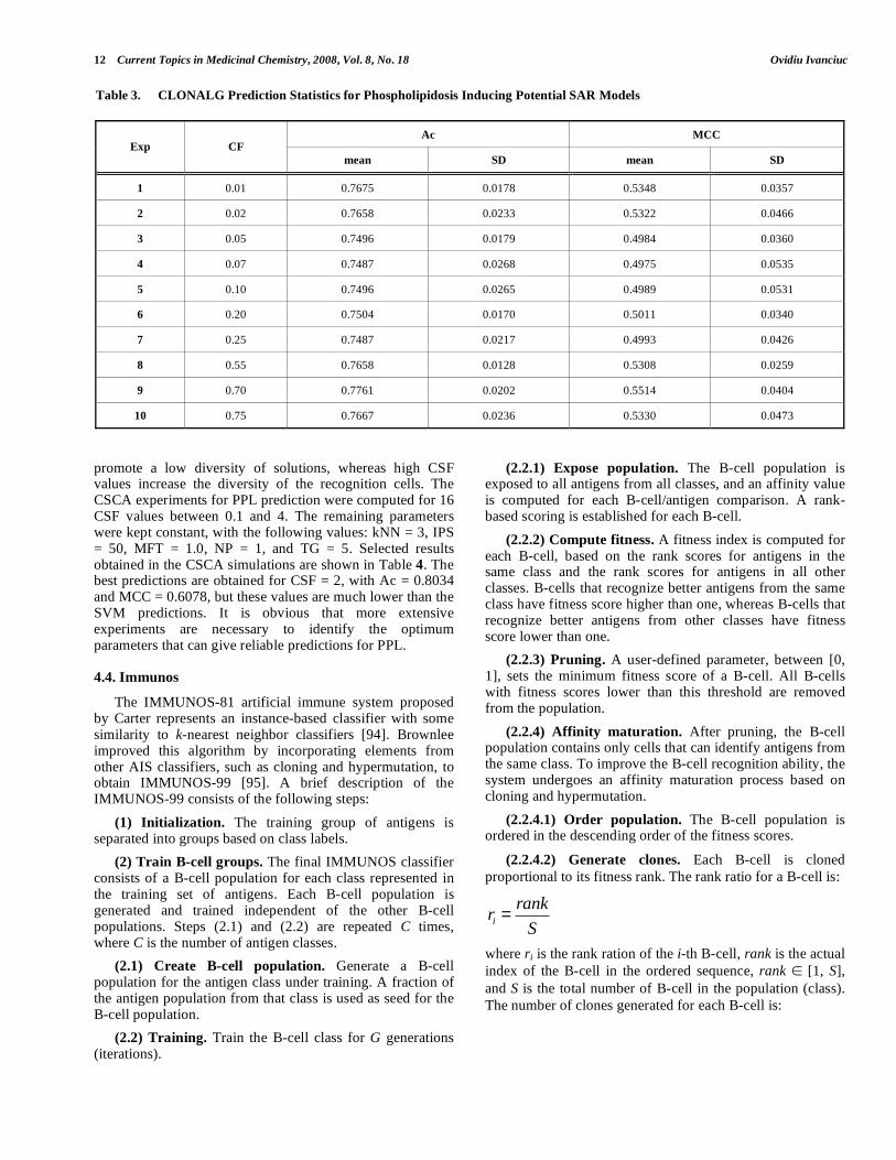
The CLONALG machine learning was tested with success in drug design and structure-activity applications, namely for the classification of benzodiazepine receptor ligands [117], for the recognition of glycogen phosphorylase B inhibitors [118], and to identify polar and nonpolar narcotic pollutants [119]. The classification performance of the CLONALG algorithm depends on six user defined parameters: clonal factor CF, antibody pool size APS, number of generations NG, remainder pool ratio RPR, selection pool size SPS, and total replacements TR. To illustrate the effect of the user defined parameters on the prediction performance of CLONALG, we show the influence of the clonal factor CF on the prediction of the phospholipidosis inducing potential. The clonal factor is a scaling factor, with values between 0 and 1, which determines the number of clones generated for each selected antibody. Low values for CF result in a local search, whereas for high values the algorithm generates a larger number of clones that may explore a wider region and result in a higher diversity. The CLONALG experiments for PPL prediction were computed for 27 CF values between 0.01 and 0.95. The remaining parameters were kept constant, with the following values: APS = 50, NG = 10, RPR = 0.1, SPS = 20, and TR = 2.

In Table 3 we present several representative results for the CLONALG simulations. The best predictions are obtained for CF = 0.7, with Ac = 0.7761 and MCC = 0.5514, which is significantly below the SVM predictions. These results suggest that a complete optimization of all parameters might be necessary in order to obtain useful predictions for PPL. CLONALG is a relatively new addition to the machine learning collection of algorithms, and there is limited information regarding the best strategy to follow to obtain reliable models.

4.3. CSCA - Clonal Selection Classification System

The clonal selection classification system CSCA was developed by Brownlee, and is formulated as a function optimization procedure that maximizes the number of patterns correctly classified and minimizes the number of patterns incorrectly classified [86]. CSCA is trained for several generations, and during each generation the entire set of antibodies is exposed to all antigens. The CSCA algorithm consists of the following steps:

(1) Initialization. Generate a set of N antibodies.

(2) Training. Repeat the training of all antibodies for G generations (iterations).

(2.1) Selection and pruning. The entire group of antibodies is exposed to the antigen set and a fitness score is computed for each antibody. Then all antibodies are selected and the following three evaluation rules are applied to each antibody:

(2.1.1) Remove from the selected set all antibodies with a misclassification score of zero.

(2.1.2) Antibodies that have zero correct classification and misclassification higher than zero are reassigned to the class of the majority, and the fitness is recalculated.

(2.1.3) Remove from the selected set and from the base antibody population all antibodies with a fitness scoring lower than a threshold.

(2.2) Cloning and mutation. The selected set of antibodies is cloned and mutated.

(2.3) Insert new antibodies. Insert the clones generated into the main antibody population. A number of n randomly selected antigens from the antigen set are inserted into the main antibody population, where n is the number of antibodies selected in step (2.1).

(3) Final pruning. The antibody population is exposed to the entire antigen population, fitness scores are computed for each antibody, and pruning of antibodies is performed as described in step (2.1.3).

(4) Select classifier. The final antibody population represents the CSCA classifier. To classify a new object, the classification antibodies are exposed to that object, then the k most similar (highest affinity) antibodies are selected and a majority vote assigns the class of the object.

CSCA was applied in several structure-activity studies, namely for the classification of thermolysin inhibitors [120], identification of dihydrofolate reductase inhibitors [121], recognition of estrogen receptor ligands [122], and classification of angiotensin converting enzyme inhibitors [123]. The classification performance of the CSCA immune system depends on six parameters that are set by the user: clonal scale factor CSF, number of nearest neighbors kNN, initial population size IPS, minimum fitness threshold MFT, number of partitions NP, and total generations TG. To demonstrate the influence of the user defined parameters on the CSCA predictions, we evaluate the influence of the clonal scale factor CSF on PPL predictions. CSF is used to increase or decrease the number of clones generated for each antibody, and has a default value of one. Low values for CSF


promote a low diversity of solutions, whereas high CSF values increase the diversity of the recognition cells. The CSCA experiments for PPL prediction were computed for 16 CSF values between 0.1 and 4. The remaining parameters were kept constant, with the following values: kNN = 3, IPS = 50, MFT = 1.0, NP = 1, and TG = 5. Selected results obtained in the CSCA simulations are shown in Table 4. The best predictions are obtained for CSF = 2, with Ac = 0.8034 and MCC = 0.6078, but these values are much lower than the SVM predictions. It is obvious that more extensive experiments are necessary to identify the optimum parameters that can give reliable predictions for PPL.

4.4. Immunos

The IMMUNOS-81 artificial immune system proposed by Carter represents an instance-based classifier with some similarity to k-nearest neighbor classifiers [94]. Brownlee improved this algorithm by incorporating elements from other AIS classifiers, such as cloning and hypermutation, to obtain IMMUNOS-99 [95]. A brief description of the IMMUNOS-99 consists of the following steps:

(1) Initialization. The training group of antigens is separated into groups based on class labels.

(2) Train B-cell groups. The final IMMUNOS classifier consists of a B-cell population for each class represented in the training set of antigens. Each B-cell population is generated and trained independent of the other B-cell populations. Steps (2.1) and (2.2) are repeated C times, where C is the number of antigen classes.

(2.1) Create B-cell population. Generate a B-cell population for the antigen class under training. A fraction of the antigen population from that class is used as seed for the B-cell population.

(2.2) Training. Train the B-cell class for G generations (iterations).

(2.2.1) Expose population. The B-cell population is exposed to all antigens from all classes, and an affinity value is computed for each B-cell/antigen comparison. A rank-based scoring is established for each B-cell.

(2.2.2) Compute fitness. A fitness index is computed for each B-cell, based on the rank scores for antigens in the same class and the rank scores for antigens in all other classes. B-cells that recognize better antigens from the same class have fitness score higher than one, whereas B-cells that recognize better antigens from other classes have fitness score lower than one.

(2.2.3) Pruning. A user-defined parameter, between [0, 1], sets the minimum fitness score of a B-cell. All B-cells with fitness scores lower than this threshold are removed from the population.

(2.2.4) Affinity maturation. After pruning, the B-cell population contains only cells that can identify antigens from the same class. To improve the B-cell recognition ability, the system undergoes an affinity maturation process based on cloning and hypermutation.

(2.2.4.1) Order population. The B-cell population is ordered in the descending order of the fitness scores.

(2.2.4.2) Generate clones. Each B-cell is cloned

proportional to its fitness rank. The rank ratio for a B-cell is:

ri =rank

S

where ri is the rank ration of the i-th B-cell, rank is the actual

index of the B-cell in the ordered sequence, rank [1, S],

and S is the total number of B-cell in the population (class).

The number of clones generated for each B-cell is:

Table 3. CLONALG Prediction Statistics for Phospholipidosis Inducing Potential SAR Models

Ac MCC Exp CF

mean SD mean SD

1 0.01 0.7675 0.0178 0.5348 0.0357

2 0.02 0.7658 0.0233 0.5322 0.0466

3 0.05 0.7496 0.0179 0.4984 0.0360

4 0.07 0.7487 0.0268 0.4975 0.0535

5 0.10 0.7496 0.0265 0.4989 0.0531

6 0.20 0.7504 0.0170 0.5011 0.0340

7 0.25 0.7487 0.0217 0.4993 0.0426

8 0.55 0.7658 0.0128 0.5308 0.0259

9 0.70 0.7761 0.0202 0.5514 0.0404

10 0.75 0.7667 0.0236 0.5330 0.0473


NCi =ri

rj

j=1

SN + 0.5

where N is the total number of antigens in the same class.

(2.2.4.3) Mutate clones. The clones are mutated by the

inverse of the B-cell rank ratios. As a result of this

procedure, clones of B-cells with higher ranks undergo small

mutations, whereas clones of B-cells with lower ranks go

through large mutations. All clones generated are added to

the B-cell population.

(2.2.5) Insert random antigens. In order to increase the diversity of the B-cell population, a random selection of antigens from the same class is added to the B-cell pool. The number of antigens added is equal to the number of B-cells deleted during the pruning process from step (2.2.3). The diversity introduced by the antigen-based B-cells is particularly useful whenever the affinity maturation process converges to a limited number of B-cells.

(3) Final pruning. This step removes B-cells with low fitness after the system finishes the training for each antigen class and for the set number of generations G.

(3.1) Compute fitness. Each B-cell population (class) is exposed to all antigens, one antigen at a time, and only the best matching B-cells receive a score.

(3.2) Pruning. Similarly with the pruning process from step (2.2.3), all B-cells with low fitness scores lower are removed from the population.

(4) Select classifier. The populations of B-cells that survive the final pruning represent the classifier for new, unknown antigens. During the classification process, each B-cell class is exposed to the unknown antigen, and an avidity index is computed. Then the B-cell populations compete for

the unknown antigen that takes the class label of the B-cell population with the highest avidity index.

The IMMUNOS-99 immune system was applied to several structure-activity studies, namely recognition of benzodiazepine receptor ligands [117], SAR models for acetylcholinesterase inhibitors [124], classification of thrombin inhibitors [125], and virtual screening of cyclooxygenase-2 inhibitors [126]. IMMUNOS-99 has three parameters that control the classification performance: seed population percentage SPP, minimum fitness threshold MFT, and total generations TG. The experiments presented here investigate the influence of the seed population percentage. SPP represents the percentage of the antigen population from each class that is used as seed for the B-cell population. If SPP = 100% then the initial B-cell population is identical with the antigen population in the same class. The IMMUNOS-99 classifier was trained for 19 values of the SPP parameter, between 0.05 and 0.95, with MFT = 0.5 and TG = 2. Overall, the predictions are lower than those obtained with AIRS, CLONALG, and CSCA, as shown by the selected results presented in Table 6. The best predictions are obtained for SPP = 0.6, with Ac = 0.6641 and MCC = 0.4503, but such low values are not useful for PPL prediction.

5. PHOSPHOLIPIDOSIS PREDICTION WITH OTHER MACHINE LEARNING ALGORITHMS

In this section we present a large scale comparison of Weka machine learning algorithms that are trained to identify drugs with phospholipidosis inducing potential. These experiments will be compared with the results obtained with SVM and AIS models. The machine learning algorithms used are briefly listed here, using their notation in Weka: BayesNet, Bayesian network; NaiveBayes, naïve Bayesian classifier [127]; NaiveBayesUpdateable, naïve Bayesian classifier with estimator classes [127]; Logistic, logistic regression with a ridge estimator [128]; Multilayer Perceptron, multiplayer perceptron artificial neural network

Table 4. CSCA Prediction Statistics for Phospholipidosis Inducing Potential SAR Models

Ac MCC Exp CSF

mean SD mean SD

1 0.1 0.8000 0.0134 0.6016 0.0259

2 0.2 0.8017 0.0161 0.6034 0.0324

3 0.4 0.8026 0.0224 0.6057 0.0447

4 0.5 0.7940 0.0124 0.5886 0.0248

5 0.6 0.7932 0.0178 0.5866 0.0356

6 0.9 0.7932 0.0190 0.5867 0.0388

7 1.0 0.7991 0.0122 0.5993 0.0249

8 1.5 0.7940 0.0145 0.5889 0.0297

9 2.0 0.8034 0.0121 0.6078 0.0230

10 4.0 0.7932 0.0212 0.5877 0.0435


Table 5. IMMUNOS Prediction Statistics for Phospholipidosis Inducing Potential SAR Models

Ac MCC Exp SPP

mean SD mean SD

1 0.05 0.6504 0.0355 0.3721 0.0811

2 0.10 0.6402 0.0200 0.3978 0.0320

3 0.15 0.6410 0.0245 0.4079 0.0443

4 0.20 0.6368 0.0168 0.4036 0.0395

5 0.30 0.6444 0.0134 0.4159 0.0261

6 0.60 0.6641 0.0094 0.4503 0.0200

7 0.65 0.6632 0.0139 0.4455 0.0255

8 0.70 0.6650 0.0142 0.4432 0.0283

9 0.90 0.6624 0.0149 0.4427 0.0313

10 0.95 0.6650 0.0126 0.4450 0.0241

Table 6. Machine Learning Prediction Statistics for Phospholipidosis Inducing Potential SAR

Ac MCC Exp Machine Learning

mean SD mean SD

1 SVM RBF =0.01 0.9701 0.0043 0.9413 0.0085

2 SVM tanh a=0.10 b=0.25 0.9513 0.0094 0.9032 0.0186

3 MultilayerPerceptron h = 0 0.9359 0.0079 0.8717 0.0156

4 SVM linear 0.9120 0.0195 0.8237 0.0391

5 SimpleLogistic 0.8863 0.0108 0.7726 0.0217

6 LWL SimpleLogistic 0.8855 0.0210 0.7711 0.0422

7 LWL Logistic 0.8709 0.0118 0.7444 0.0228

8 IBk k = 7 W(1/d) 0.8530 0.0100 0.7103 0.0197

9 RBFNetwork C = 2 0.8462 0.0223 0.6959 0.0462

10 Logistic 0.8453 0.0124 0.6938 0.0270

11 LWL IBk k = 3 NoW 0.8462 0.0158 0.6930 0.0322

12 LWL NaiveBayes 0.8462 0.0108 0.6919 0.0216

13 AIRS ATS=0.08 0.8385 0.0323 0.6788 0.0640

14 RandomForest T = 50 0.8282 0.0135 0.6568 0.0278

15 NaiveBayes 0.8274 0.0120 0.6551 0.0243

16 NaiveBayesUpdateable 0.8274 0.0120 0.6551 0.0243

17 ADTree Erp 0.8239 0.0227 0.6487 0.0455

18 LWL ADTree 0.8222 0.0232 0.6449 0.0461

19 NBTree 0.8145 0.0377 0.6296 0.0755

20 LWL DecisionStump 0.8120 0.0066 0.6241 0.0131

21 LWL RandomForest T = 10 0.8077 0.0239 0.6190 0.0462


(Table 6) Contd…..

Ac MCC Exp Machine Learning

mean SD mean SD

22 CSCA CSF=2.0 0.8034 0.0121 0.6078 0.0230

23 DecisionStump 0.8000 0.0109 0.6014 0.0209

24 BayesNet 0.7940 0.0140 0.5936 0.0255

25 KStar 0.7923 0.0162 0.5885 0.0326

26 REPTree 0.7829 0.0217 0.5685 0.0412

27 SimpleCart 0.7829 0.0248 0.5661 0.0498

28 NNge 0.7812 0.0192 0.5625 0.0398

29 PART 0.7769 0.0349 0.5542 0.0693

30 OneR 0.7744 0.0167 0.5515 0.0331

31 CLONALG CF=0.70 0.7761 0.0202 0.5514 0.0404

32 Ridor 0.7726 0.0342 0.5449 0.0682

33 J48 0.7709 0.0288 0.5447 0.0581

34 ConjunctiveRule 0.7641 0.0271 0.5309 0.0538

35 BFTree 0.7641 0.0172 0.5280 0.0344

36 JRip 0.7632 0.0202 0.5276 0.0417

37 LWL J48 0.7556 0.0245 0.5111 0.0496

38 VotedPerceptron 0.7350 0.0276 0.4967 0.0526

39 DecisionTable 0.7427 0.0287 0.4891 0.0569

40 IMMUNOS SPP=0.60 0.6641 0.0094 0.4503 0.0200

41 RandomTree 0.7214 0.0522 0.4435 0.1030

42 LWL RandomTree 0.7188 0.0263 0.4388 0.0525

43 FLR 0.7128 0.0245 0.4264 0.0510

44 HyperPipes 0.6991 0.0283 0.4117 0.0575

45 VFI 0.6803 0.0199 0.4060 0.0393

(h = number of hidden neurons, h = 0 to 3); RBFNetwork, Gaussian radial basis function network (C = number of clusters, C = 2 to 6); SimpleLogistic; VotedPerceptron; IBk, k-NN classifier with distance weight (NoW = no distance weight, W(1/d) = weighted with 1/d, W(1-d) = weighted with (1-d)) and k an odd number between 1 and 9 [129]; KStar, K* lazy learner with entropy-based distance function [130]; LWL, locally weighted learning coupled with a base classifier; FLR; HyperPipes; VFI; ADTree, alternating decision tree (search type: Eap, expand all paths; Ehp, expand the heaviest path; Ezp, expand the best z-pure path; Erp, expand a random path) [131]; BFTree; DecisionStump, one-level binary decision tree with categorical or numerical class label; J48, C4.5 decision tree [132]; NBTree, decision tree with naïve Bayes classifiers at the leaves [133]; RandomForest, random forest (T = number of random trees, T = 10 to 50) [134]; RandomTree, a tree that considers k

randomly chosen attributes at each node; REPTree, fast decision tree learner; SimpleCart; ConjunctiveRule, conjunc-tive rule learner; DecisionTable, decision table majority classifier [135]; JRip, a propositional rule learner based on RIPPER [136]; Nnge; OneR, rule classifier that uses the minimum-error attribute for prediction [137]; PART, a PART decision list that builds a partial C4.5 decision tree in each iteration and transforms the best leaf into a rule ; Ridor, a RIpple-DOwn Rule learner [138]. More details for each ML may be found in Weka.

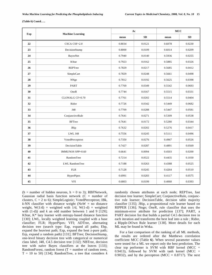
For a fast comparison of the ranking of all ML methods, the results are ordered after the Matthews correlation coefficient MCC (Table 6). When several parameter values were tested for a ML we report only the best prediction. The clear top performer is SVM with RBF kernel (MCC = 0.9413), followed by SVM with tanh kernel (MCC = 0.9032), and by the perceptron (MCC = 0.8717). The next


places are occupied by the linear SVM followed by three classifiers based on logistic regression. Although we have investigated a large diversity of ML algorithms, we did not find any real competitor for the SVM with RBF kernel. The classification statistics of the SVM with RBF kernel are high enough to be of real use in identifying drugs with phospholipidosis inducing potential.

6. CONCLUSIONS

Phospholipidosis is a serious side effect caused by some cationic amphiphilic drugs, in which phospholipids are accumulated in the cells and form concentric lamellar bodies. Large amounts of phospholipids may accumulate in the liver, lungs, or kidneys, and may compromise their normal function. Phospholipidosis is especially problematic when drugs are taken for a long period of time that results in larger accumulation of phospholipids in the cells. In this paper we have presented a large-scale application of machine learning algorithms computed with Weka for the prediction of the phospholipidosis inducing potential of drugs. This structure-activity study is the largest comparative evaluation of machine learning for PPL prediction, and represents an important step in identifying the best ML algorithms that can be used for the high throughput screening of drug candidates. By far the best predictions were obtained with a support vector machine with RBF kernel that has a prediction accuracy of 97%. Extensive computational experiments show that for a given property, the best SAR model may be identified only by an empirical comparison of a large number of ML methods. Weka represents a very efficient environment for testing and comparing machine learning algorithms, with potential applications in drug design and discovery.

7. REFERENCES

[1] Berndt, E. R.; Gottschalk, A. H. B.; Strobeck, M. W. Opportunities for improving the drug development process: Results from a survey of industry and the FDA. In National Bureau of Economic Research Workshop on Innovation Policy and the Economy, NBER Working Paper No. 11425: Washington, DC, 2005.

[2] Keyhani, S.; Diener-West, M.; Powe, N. Are development times for pharmaceuticals increasing or decreasing? Health Aff. 2006, 25, 461-468.

[3] DiMasi, J. A.; Hansen, R. W.; Grabowski, H. G. The price of innovation: new estimates of drug development costs. J. Health

Econ. 2003, 22, 151-185. [4] Adams, C. P.; Brantner, V. V. Estimating the cost of new drug

development: is it really 802 million dollars? Health Aff. 2006, 25, 420-428.

[5] Kola, I.; Landis, J. Can the pharmaceutical industry reduce attrition rates? Nat. Rev. Drug Discov. 2004, 3, 711-715.

[6] Lasser, K. E.; Allen, P. D.; Woolhandler, S. J.; Himmelstein, D. U.; Wolfe, S. N.; Bor, D. H. Timing of new black box warnings and withdrawals for prescription medications. J. Am. Med. Assoc. 2002, 287, 2215-2220.

[7] Faich, G. A.; Moseley, R. H. Troglitazone (Rezulin) and hepatic injury. Pharmacoepidemiol. Drug Saf. 2001, 10, 537-547.

[8] Furberg, C. D.; Pitt, B. Withdrawal of cerivastatin from the world market. Curr. Control Trials Cardivasc. Med. 2001, 2, 205-207.

[9] Dieppe, P. A.; Ebrahim, S.; Martin, R. M.; Jüni, P. Lessons from the withdrawal of rofecoxib. Br. Med. J. 2004, 329, 867-868.

[10] Hansch, C. A quantitative approach to biochemical structure-activity relationships. Acc. Chem. Res. 1969, 2, 232-239.

[11] Boid, D. B. How computational chemistry became important in the pharmaceutical industry. In Reviews in Computational Chemistry, Lipkowitz, K. B.; Cundari, T. R., Eds. Wiley-VCH: Weinheim, 2007; Vol. 23, pp 401-451.

[12] Hansch, C.; Maloney, P. P.; Fujita, T.; Muir, R. M. Correlation of biological activity of phenoxyacetic acids with Hammett substi-tuent constants and partition coefficients. Nature 1962, 194, 178-180.

[13] Hansch, C.; Fujita, T. - - analysis. A method for the correlation of biological activity and chemical structure. J. Am. Chem. Soc. 1964, 86, 1616-1626.

[14] Fujita, T.; Iwasa, J.; Hansch, C. A new substituent constant, , derived from partition coefficients. J. Am. Chem. Soc. 1964, 86, 5175-5180.

[15] Bonchev, D.; Rouvray, D. H. Chemical Graph Theory.

Introduction and Fundamentals. Abacus Press/Gordon & Breach Science Publishers: New York, 1991.

[16] Trinajsti , N. Chemical Graph Theory. CRC Press: Boca Raton, FL, 1992.

[17] Ivanciuc, O. Graph theory in chemistry. In Handbook of Chemoinformatics, Gasteiger, J., Ed. Wiley-VCH: Weinheim, 2003; Vol. 1, pp 103-138.

[18] Bonchev, D. Information Theoretic Indices for Characterization of

Chemical Structure. Research Studies Press: Chichester, UK, 1983. [19] Balaban, A. T.; Ivanciuc, O. Historical development of topological

indices. In Topological Indices and Related Descriptors in QSAR and QSPR, Devillers, J.; Balaban, A. T., Eds. Gordon and Breach Science Publishers: Amsterdam, 1999; pp 21-57.

[20] Ivanciuc, O. Topological indices. In Handbook of Chemoin-

formatics, Gasteiger, J., Ed. Wiley-VCH: Weinheim, 2003; Vol. 3, pp 981-1003.

[21] Kier, L. B.; Hall, L. H. Molecular Connectivity in Chemistry and Drug Research. Academic Press: New York, 1976.

[22] Kier, L. B.; Hall, L. H. Molecular Connectivity in Structure-Activity Analysis. Research Studies Press: Letchworth, 1986.

[23] Kier, L. B.; Hall, L. H. Molecular Structure Description. The Electrotopological State. Academic Press: San Diego, 1999.

[24] Ivanciuc, O. Electrotopological state indices. In Molecular Drug Properties. Measurement and Prediction, Mannhold, R., Ed. Wiley-VCH: Weinheim, 2008; pp 85-109.

[25] Todeschini, R.; Consonni, V. Descriptors from molecular geometry. In Handbook of Chemoinformatics, Gasteiger, J., Ed. Wiley-VCH: Weinheim, 2003; Vol. 3, pp 1004-1033.

[26] Jurs, P. Quantitative structure-property relationships. In Handbook of Chemoinformatics, Gasteiger, J., Ed. Wiley-VCH: Weinheim, 2003; Vol. 3, pp 1314-1335.

[27] Ivanciuc, O. 3D QSAR models. In QSPR/QSAR Studies by

Molecular Descriptors, Diudea, M. V., Ed. Nova Science Publishers: Huntington, NY, 2001; pp 233-280.

[28] Ivanciuc, T.; Ivanciuc, O.; Klein, D. J. Posetic quantitative superstructure/activity relationships (QSSARs) for chlorobenzenes. J. Chem. Inf. Model. 2005, 45, 870-879.

[29] Ivanciuc, T.; Ivanciuc, O.; Klein, D. J. Modeling the bioconcen-tration factors and bioaccumulation factors of polychlorinated biphenyls with posetic quantitative super-structure/activity relationships (QSSAR). Mol. Divers. 2006, 10, 133-145.

[30] Ivanciuc, T.; Ivanciuc, O.; Klein, D. J. Prediction of environmental properties for chlorophenols with posetic quantitative super-structure/property relationships (QSSPR). Int. J. Mol. Sci. 2006, 7, 358-374.

[31] González-Díaz, H.; González-Díaz, Y.; Santana, L.; Ubeira, F. M.; Uriarte, E. Proteomics, networks and connectivity indices. Proteomics 2008, 8, 750-778.

[32] Goulon-Sigwalt-Abram, A.; Duprat, A.; Dreyfus, G. From Hopfield nets to recursive networks to graph machines: Numerical machine learning for structured data. Theor. Comput. Sci. 2005, 344, 298-334.

[33] Ivanciuc, O. New neural networks for structure-property models. In QSPR/QSAR Studies by Molecular Descriptors, Diudea, M. V., Ed. Nova Science Publishers: Huntington, NY, 2001; pp 213-231.

[34] Baldi, P.; Pollastri, G. The principled design of large-scale recursive neural network architectures-DAG-RNNs and the protein structure prediction problem. J. Mach. Learn. Res. 2004, 4, 575-602.

[35] Micheli, A.; Portera, F.; Sperduti, A. A preliminary empirical comparison of recursive neural networks and tree kernel methods on regression tasks for tree structured domains. Neurocomputing

2005, 64, 73-92. [36] Baskin, I. I.; Palyulin, V. A.; Zefirov, N. S. A neural device for

searching direct correlations between structures and properties of


chemical compounds. J. Chem. Inf. Comput. Sci. 1997, 37, 715-721.

[37] Kireev, D. B. ChemNet: A novel neural network based method for graph/property mapping. J. Chem. Inf. Comput. Sci. 1995, 35, 175-180.

[38] Ivanciuc, O. Artificial neural networks applications. Part 9. MolNet prediction of alkane boiling points. Rev. Roum. Chim. 1998, 43, 885-894.

[39] Ivanciuc, O. The neural network MolNet prediction of alkane enthalpies. Anal. Chim. Acta 1999, 384, 271-284.

[40] Zhang, S.; Golbraikh, A.; Oloff, S.; Kohn, H.; Tropsha, A. A novel automated lazy learning QSAR (ALL-QSAR) approach: Method development, applications, and virtual screening of chemical databases using validated ALL-QSAR models. J. Chem. Inf. Model. 2006, 46, 1984-1995.

[41] Plewczynski, D.; von Grotthuss, M.; Spieser, S. A. H.; Rychlewski, L.; Wyrwicz, L. S.; Ginalski, K.; Koch, U. Target specific compound identification using a support vector machine. Comb. Chem. High Throughput Screen. 2007, 10, 189-196.

[42] Klon, A. E.; Diller, D. J. Library fingerprints: A novel approach to the screening of virtual libraries. J. Chem. Inf. Model. 2007, 47, 1354-1365.

[43] Vogt, M.; Bajorath, J. Introduction of an information-theoretic method to predict recovery rates of active compounds for Bayesian in silico screening: Theory and screening trials. J. Chem. Inf.

Model. 2007, 47, 337-341. [44] Schneider, N.; Jäckels, C.; Andres, C.; Hutter, M. C. Gradual in

silico filtering for druglike substances. J. Chem. Inf. Model. 2008, 48, 613-28.

[45] Frank, E.; Hall, M.; Trigg, L.; Holmes, G.; Witten, I. H. Data mining in bioinformatics using Weka. Bioinformatics 2004, 20, 2479-2481.

[46] Witten, I. H.; Frank, E. Data Mining: Practical Machine Learning

Tools and Techniques. 2 ed.; Morgan Kaufmann: San Francisco, 2005; p 525.

[47] Reasor, M. J.; Kacew, S. Drug-induced phospholipidosis: Are there functional consequences? Exp. Biol. Med. 2001, 226, 825-830.

[48] Anderson, N.; Borlak, J. Drug-induced phospholipidosis. FEBS Lett. 2006, 580, 5533-5540.

[49] Abe, A.; Hiraoka, M.; Shayman, J. A. A role for lysosomal phospholipase A2 in drug induced phospholipidosis. Drug Metab.

Lett. 2007, 1, 49-53. [50] Nonoyama, T.; Fukuda, R. Drug-induced phospholipidosis -

Pathological aspects and its prediction. J. Toxicol. Pathol. 2008, 21, 9-24.

[51] Sawada, H.; Takami, K.; Asahi, S. A toxicogenomic approach to drug-induced phospholipidosis: Analysis of its induction mechanism and establishment of a novel in vitro screening system. Toxicol. Sci. 2005, 83, 282-292.

[52] Atienzar, F.; Gerets, H.; Dufrane, S.; Tilmant, K.; Cornet, M.; Dhalluin, S.; Ruty, B.; Rose, G.; Canning, M. Determination of phospholipidosis potential based on gene expression analysis in HepG2 cells. Toxicol. Sci. 2007, 96, 101-114.

[53] Kasahara, T.; Tomita, K.; Murano, H.; Harada, T.; Tsubakimoto, K.; Ogihara, T.; Ohnishi, S.; Kakinuma, C. Establishment of an in

vitro high-throughput screening assay for detecting phos-pholipidosis-inducing potential. Toxicol. Sci. 2006, 90, 133-141.

[54] Vitovi , P.; Alakoskela, J. M.; Kinnunen, P. K. J. Assessment of drug-lipid complex formation by a high-throughput Langmuir-balance and correlation to phospholipidosis. J. Med. Chem. 2008, 51, 1842-1848.

[55] Ploemen, J.-P. H. T. M.; Kelder, J.; Hafmans, T.; van de Sandt, H.; van Burgsteden, J. A.; Salemink, P. J. M.; van Esch, E. Use of physicochemical calculation of pKa and CLogP to predict phospholipidosis-inducing potential. A case study with structurally related piperazines. Exp. Toxicol. Pathol. 2004, 55, 347-355.

[56] Pelletier, D. J.; Gehlhaar, D.; Tilloy-Ellul, A.; Johnson, T. O.; Greene, N. Evaluation of a published in silico model and construction of a novel Bayesian model for predicting phos-pholipidosis inducing potential. J. Chem. Inf. Model. 2007, 47, 1196-1205.

[57] Ivanciuc, O. Prediction of the phospholipidosis inducing potential with machine learning. Internet Electron. J. Mol. Des. 2007, 6, 396-402.

[58] Tomizawa, K.; Sugano, K.; Yamada, H.; Horii, I. Physicochemical and cell-based approach for early screening of phospholipidosis-inducing potential. J. Toxicol. Sci. 2006, 31, 315-324.

[59] Kruhlak, N. L.; Choi, S. S.; Contrera, J. F.; Weaver, J. L.; Willard, J. M.; Hastings, K. L.; Sancilio, L. F. Development of a phospholipidosis database and predictive quantitative structure-activity relationship (QSAR) models. Toxicol. Mech. Methods

2008, 18, 217-227. [60] Tetko, I. V.; Gasteiger, J.; Todeschini, R.; Mauri, A.; Livingstone,

D.; Ertl, P.; Palyulin, V. A.; Radchenko, E. V.; Zefirov, N. S.; Makarenko, A. S.; Tanchuk, V. Y.; Prokopenko, V. V. Virtual computational chemistry laboratory - design and description. J. Comput.-Aided Mol. Des. 2005, 19, 453-463.

[61] Ivanciuc, O. Applications of support vector machines in chemistry. In Reviews in Computational Chemistry, Lipkowitz, K. B.; Cundari, T. R., Eds. Wiley-VCH: Weinheim, 2007; Vol. 23, pp 291-400.

[62] Vapnik, V.; Lerner, A. Pattern recognition using generalized portrait method. Automat. Remote Contr. 1963, 24, 774-780.

[63] Vapnik, V. N.; Chervonenkis, A. Y. Theory of Pattern Recognition. Nauka: Moscow, 1974.

[64] Vapnik, V. N. Estimation of Dependencies Based on Empirical Data. Nauka: Moscow, 1979.

[65] Vapnik, V. N. The Nature of Statistical Learning Theory. Springer: New York, 1995.

[66] Vapnik, V. N. Statistical Learning Theory. Wiley-Interscience: New York, 1998.

[67] Boser, B. E.; Guyon, I. M.; Vapnik, V. N. In A training algorithm for optimal margin classifiers, Proceedings of the 5th Annual ACM Workshop on Computational Learning Theory, Pittsburgh, Pennsylvania, 1992; Haussler, D., Ed. ACM Press: Pittsburgh, Pennsylvania, 1992; pp 144-152.

[68] Cortes, C.; Vapnik, V. Support vector networks. Mach. Learn.

1995, 20, 273-297. [69] Schölkopf, B.; Sung, K. K.; Burges, C. J. C.; Girosi, F.; Niyogi, P.;

Poggio, T.; Vapnik, V. Comparing support vector machines with gaussian kernels to radial basis function classifiers. IEEE Trans.

Signal Process. 1997, 45, 2758-2765. [70] Vapnik, V. N. An overview of statistical learning theory. IEEE

Trans. Neural Netw. 1999, 10, 988-999. [71] Vapnik, V.; Chapelle, O. Bounds on error expectation for support

vector machines. Neural Comput. 2000, 12, 2013-2036. [72] Guyon, I.; Weston, J.; Barnhill, S.; Vapnik, V. Gene selection for

cancer classification using support vector machines. Mach. Learn. 2002, 46, 389-422.

[73] Schölkopf, B.; Smola, A. J. Learning with Kernels. MIT Press: Cambridge, MA, 2002.

[74] Herbrich, R. Learning Kernel Classifiers. MIT Press: Cambridge, MA, 2002.

[75] Cristianini, N.; Shawe-Taylor, J. An Introduction to Support Vector Machines. Cambridge University Press: Cambridge, 2000.

[76] Schölkopf, B.; Burges, C. J. C.; Smola, A. J. Advances in Kernel Methods: Support Vector Learning. MIT Press: Cambridge, MA, 1999.

[77] de Castro, L. N.; Timmis, J. I. Artificial immune systems as a novel soft computing paradigm. Soft Comput. 2003, 7, 526-544.

[78] Musilek, P.; Lau, A.; Reformat, M.; Wyard-Scott, L. Immune programming. Inf. Sci. 2006, 176, 972-1002.

[79] Timmis, J. Artificial immune systems - Today and tomorrow. Nat.

Comput. 2007, 6, 1-18. [80] Forrest, S.; Beauchemin, C. Computer immunology. Immunol. Rev.

2007, 216, 176-197. [81] de Castro, L. N.; Von Zuben, F. J. Artificial immune systems: Part I

- Basic theory and applications; Technical Report TR DCA 01/99; FEEC/UNICAMP, Brazil: 1999.

[82] de Castro, L. N.; Von Zuben, F. J. Artificial immune systems: Part II - A survey of applications; Technical Report TR DCA 02/00; FEEC/UNICAMP, Brazil: 2000.

[83] Timmis, J.; Neal, M.; Hunt, J. An artificial immune system for data analysis. BioSystems 2000, 55, 143-150.

[84] de Castro, L. N.; Von Zuben, F. J. The clonal selection algorithm with engineering applications. In GECCO-2000: Proceedings of the Genetic and Evolutionary Computation Conference, July 10-12,

2000, Las Vegas, Nevada, Whitley, D.; Goldberg, D.; Cantu-Paz, E.; Spector, L.; Parmee, I.; Beyer, H.-G., Eds. Morgan Kaufmann: San Francisco, CA, 2000; pp 36-37.


[85] de Castro, L. N.; Von Zuben, F. J. Learning and optimization using the clonal selection principle. IEEE Trans. Evol. Comput. 2002, 6, 239-251.

[86] Brownlee, J. Clonal selection theory & CLONAG. The clonal selection classification algorithm (CSCA); Technical Report No. 2-02; Centre for Intelligent Systems and Complex Processes (CISCP), Faculty of Information and Communication Technologies (ICT), Swinburne University of Technology (SUT), Victoria, Australia: 2005.

[87] Watkins, A.; Timmis, J.; Boggess, L. Artificial immune recognition system (AIRS): An immune-inspired supervised learning algorithm. Genet. Programm. Evolv. Mach. 2004, 5, 291-317.

[88] Meng, L.; van der Putten, P.; Wang, H. A comprehensive benchmark of the artificial immune recognition system (AIRS). In Advanced Data Mining and Applications, Proceedings, 2005; Vol. 3584, pp 575-582.

[89] Watkins, A. B. AIRS: A resource limited artificial immune classifier. Mississippi State University, 2001.

[90] Watkins, A. B. Exploiting immunological metaphors in the development of serial, parallel and distributed learning algorithms. University of Kent, Canterbury, UK, 2005.

[91] de Castro, L. N. Dynamics of an artificial immune network. J. Exp. Theor. Artif. Intell. 2004, 16, 19-39.

[92] Bezerra, G. B.; de Castro, L. N.; Von Zuben, F. J. A hierarchical immune network applied to gene expression data. In Artificial

Immune Systems: Third International Conference, ICARIS 2004, Catania, Sicily, Italy, September 13-16, 2004, Nicosia, G.; Cutello, V.; Bentley, P. J.; Timmis, J. I., Eds. Springer-Verlag: Berlin, 2004; Vol. 3239, pp 14-27.

[93] Bezerra, G. B.; Cançado, G. M. A.; Menossi, M.; de Castro, L. N.; Von Zuben, F. J. Recent advances in gene expression data clustering: A case study with comparative results. Genet. Mol. Res. 2005, 4, 514-524.

[94] Carter, J. H. The immune system as a model for pattern recognition and classification. J. Am. Med. Inf. Assoc. 2000, 7, 28-41.

[95] Brownlee, J. Immunos-81. The misunderstood artificial immune system; Technical Report No. 3-01; Centre for Intelligent Systems and Complex Processes (CISCP), Faculty of Information and Communication Technologies (ICT), Swinburne University of Technology (SUT), Victoria, Australia: 2005.

[96] Ando, S.; Iba, H. Artificial immune system for classification of cancer. In Applications of Evolutionary Computing, 2003; Vol. 2611, pp 1-10.

[97] Tsankova, D.; Georgieva, V.; Kasabov, N. Artificial immune networks as a paradigm for classification and profiling of gene expression data. J. Comput. Theor. Nanosci. 2005, 2, 543-550.

[98] Polat, K.; ahan, S.; Kodaz, H.; Güne , S. Breast cancer and liver disorders classification using artificial immune recognition system (AIRS) with performance evaluation by fuzzy resource allocation mechanism. Expert Syst. Appl. 2007, 32, 172-183.

[99] ahan, S.; Polat, K.; Kodaz, H.; Güne , S. A new hybrid method based on fuzzy-artificial immune system and k-nn algorithm for breast cancer diagnosis. Comput. Biol. Med. 2007, 37, 415-423.

[100] Polat, K.; Güne , S. Principles component analysis, fuzzy weighting pre-processing and artificial immune recognition system based diagnostic system for diagnosis of lung cancer. Expert Syst. Appl. 2008, 34, 214-221.

[101] Polat, K.; Güne , S. Computer aided medical diagnosis system based on principal component analysis and artificial immune recognition system classifier algorithm. Expert Syst. Appl. 2008, 34, 773-779.

[102] Polat, K.; Güne , S. Medical decision support system based on artificial immune recognition immune system (AIRS), fuzzy weighted pre-processing and feature selection. Expert Syst. Appl. 2007, 33, 484-490.

[103] Polat, K.; Güne , S.; Tosun, S. Diagnosis of heart disease using artificial immune recognition system and fuzzy weighted pre-processing. Pattern Recognit. 2006, 39, 2186-2193.

[104] Polat, K.; ahan, S.; Güne , S. Automatic detection of heart disease using an artificial immune recognition system (AIRS) with fuzzy resource allocation mechanism and k-nn (nearest neighbour) based weighting preprocessing. Expert Syst. Appl. 2007, 32, 625-631.

[105] Polat, K.; ahan, S.; Güne , S. A new method to medical diagnosis: Artificial immune recognition system (AIRS) with fuzzy weighted pre-processing and application to ECG arrhythmia. Expert Syst.

Appl. 2006, 31, 264-269.

[106] Polat, K.; ahan, S.; Güne , S. A novel hybrid method based on artificial immune recognition system (AIRS) with fuzzy weighted pre-processing for thyroid disease diagnosis. Expert Syst. Appl.

2007, 32, 1141-1147. [107] Latifoglu, F.; ahan, S.; Kara, S.; Güne , S. Diagnosis of

atherosclerosis from carotid artery Doppler signals as a real-world medical application of artificial immune systems. Expert Syst.

Appl. 2007, 33, 786-793. [108] Cutello, V.; Nicosia, G.; Pavone, M. In An immune algorithm with

hyper-macromutations for the Dill's 2D hydrophobic-hydrophilic model, Congress on Evolutionary Computation, CEC2004, 2004; 2004; pp 1074-1080.

[109] Cutello, V.; Nicosia, G.; Pavone, M.; Timmis, J. An immune algorithm for protein structure prediction on lattice models. IEEE Trans. Evol. Comput. 2007, 11, 101-117.

[110] Anile, A. M.; Cutello, V.; Narzisi, G.; Nicosia, G.; Spinella, S. Determination of protein structure and dynamics combining immune algorithms and pattern search methods. Nat. Comput. 2007, 6, 55-72.

[111] Watkins, A.; Timmis, J. In Artificial immune recognition system (AIRS): Revisions and refinements, Artificial Immune Systems: First International Conference, ICARIS 2002, University of Kent at Canterbury, 2002; 2002; pp 173-181.

[112] Brownlee, J. Artificial immune recognition system (AIRS). A review and analysis; Technical Report No. 1-02; Centre for Intelligent Systems and Complex Processes (CISCP), Faculty of Information and Communication Technologies (ICT), Swinburne University of Technology (SUT), Victoria, Australia: 2005.

[113] Ivanciuc, O. Artificial immune system classification of drug-induced torsade de pointes with AIRS (artificial immune recognition system). Internet Electron. J. Mol. Des. 2006, 5, 488-502.

[114] Ivanciuc, O. Artificial immune system prediction of the human intestinal absorption of drugs with AIRS (artificial immune recognition system). Internet Electron. J. Mol. Des. 2006, 5, 515-529.

[115] Ivanciuc, O. Artificial immune systems in drug design: Recognition of P-glycoprotein substrates with AIRS (artificial immune recog-nition system). Internet Electron. J. Mol. Des. 2006, 5, 542-554.

[116] Ivanciuc, O. Artificial immune systems in aquatic toxicology: Structure-activity relationships for the mechanism of toxic action with AIRS (artificial immune recognition system). Internet Electron. J. Mol. Des. 2007, 6, 13-28.

[117] Ivanciuc, O. Structure-activity relationships with artificial immune systems: Classification of benzodiazepine receptor ligands with AIRS, CLONALG, CSCA, and IMMUNOS. Internet Electron. J. Mol. Des. 2006, 5, 585-604.

[118] Ivanciuc, O. Drug design with artificial immune systems: Structure-activity relationships for glycogen phosphorylase B inhibitors with CLONALG (clonal selection algorithm). Internet Electron. J. Mol. Des. 2007, 6, 311-319.

[119] Ivanciuc, O. Structure-activity relationships in aquatic toxicology with artificial immune systems: Mechanism of toxic action classification of polar and nonpolar narcotic pollutants with CLONALG (clonal selection algorithm). Internet Electron. J. Mol.

Des. 2007, 6, 106-114. [120] Ivanciuc, O. Artificial immune systems in structure-activity

relationships: Classification of thermolysin inhibitors with CSCA (clonal selection classification system). Internet Electron. J. Mol.

Des. 2007, 6, 209-217. [121] Ivanciuc, O. Artificial immune systems in the virtual screening of

dihydrofolate reductase inhibitors with CSCA (clonal selection classification system). Internet Electron. J. Mol. Des. 2007, 6, 253-261.

[122] Ivanciuc, O. Artificial immune systems structure-activity relationships for estrogen receptor ligands with CSCA (clonal selection classification system). Internet Electron. J. Mol. Des.

2007, 6, 81-89. [123] Ivanciuc, O. Drug design with artificial immune systems:

Classification of angiotensin converting enzyme inhibitors with CSCA (clonal selection classification system). Internet Electron. J.

Mol. Des. 2007, 6, 135-143. [124] Ivanciuc, O. Structure-activity relationships for acetylcho-

linesterase inhibitors with the IMMUNOS artificial immune system. Internet Electron. J. Mol. Des. 2007, 6, 167-175.


[125] Ivanciuc, O. Structure-activity relationships with the IMMUNOS artificial immune system for thrombin inhibitors. Internet Electron. J. Mol. Des. 2007, 6, 262-270.

[126] Ivanciuc, O. Virtual screening of cyclooxygenase-2 inhibitors with the IMMUNOS artificial immune system. Internet Electron. J. Mol.

Des. 2007, 6, 200-208. [127] John, G. H.; Langley, P. In Estimating continuous distributions in

Bayesian classifiers, UAI '95: Proceedings of the Eleventh Annual Conference on Uncertainty in Artificial Intelligence, Montreal, Quebec, Canada, August 18-20, 1995, 1995; Besnard, P.; Hanks, S., Eds. Morgan Kaufmann: Montreal, Quebec, Canada, 1995; pp 338-345.

[128] le Cessie, S.; van Houwelingen, J. C. Ridge estimators in logistic regression. Appl. Statist. 1992, 41, 191-201.

[129] Aha, D. W.; Kibler, D.; Albert, M. K. Instance-based learning algorithms. Mach. Learn. 1991, 6, 37-66.

[130] Cleary, J. G.; Trigg, L. E. In K*: An instance-based learner using

and entropic distance measure, Proceedings of the Twelfth International Conference on Machine Learning, Tahoe City, California, July 9-12, 1995, 1995; Prieditis, A.; Russell, S. J., Eds. Morgan Kaufmann: Tahoe City, California, 1995; pp 108-114.

[131] Freund, Y.; Mason, L. In The alternating decision tree learning algorithm, Proceedings of the Sixteenth International Conference

on Machine Learning (ICML 1999), Bled, Slovenia, June 27-30, 1999, 1999; Bratko, I.; Dzeroski, S., Eds. Morgan Kaufmann: Bled, Slovenia, 1999; pp 124-133.

[132] Quinlan, R. C4.5: Programs for Machine Learning. Morgan Kaufmann: San Mateo, CA, 1993.

[133] Kohavi, R. In Scaling up the accuracy of naive-Bayes classifiers: A decision-tree hybrid, Proceedings of the Second International Conference on Knowledge Discovery and Data Mining (KDD-96), 1996; Simoudis, E.; Han, J.; Fayyad, U. M., Eds. AAAI Press: 1996; pp 202-207.

[134] Breiman, L. Random forests. Mach. Learn. 2001, 45, 5-32. [135] Kohavi, R. In The power of decision tables, ECML-95, 8th

European Conference on Machine Learning, Heraclion, Crete, Greece, 1995; Lavrac, N.; Wrobel, S., Eds. Springer: Heraclion, Crete, Greece, 1995; pp 174-189.

[136] Cohen, W. W. In Fast effective rule induction, Proceedings of the Twelfth International Conference on Machine Learning, Tahoe City, California, July 9-12, 1995, 1995; Prieditis, A.; Russell, S. J., Eds. Morgan Kaufmann: Tahoe City, California, 1995; pp 115-123.

[137] Holte, R. C. Very simple classification rules perform well on most commonly used datasets. Mach. Learn. 1993, 11, 63-90.

[138] Gaines, B. R.; Compton, P. Induction of ripple-down rules applied to modeling large databases. J. Intell. Inf. Syst. 1995, 5, 211-228.

current topics in medicinal chemistry, 2008 0000 1 weka ...weka machine learning for predicting the...

Documents