currency risk factors in a recursive multi-country economy
TRANSCRIPT

Currency Risk Factors in a RecursiveMulti-Country Economy
R. Colacito M.M. Croce F. Gavazzoni R. Ready
NBER SI - International Asset Pricing
BostonJuly 8, 2015

Motivation Empirical Motivation Model Setup Model Results Conclusion
Motivation
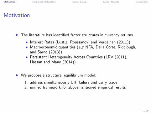
I The literature has identified factor structures in currency returns
• Interest Rates (Lustig, Roussanov, and Verdelhan (2011))• Macroeconomic quantities (e.g NFA, Della Corte, Riddiough,
and Sarno (2013))• Persistent Heterogeneity Across Countries (LRV (2011),
Hassan and Mano (2014))
I We propose a structural equilibrium model:
1. address simultaneously UIP failure and carry trade2. unified framework for abovementioned empirical results
1 / 29
Motivation Empirical Motivation Model Setup Model Results Conclusion
Motivation
I The literature has identified factor structures in currency returns
• Interest Rates (Lustig, Roussanov, and Verdelhan (2011))• Macroeconomic quantities (e.g NFA, Della Corte, Riddiough,
and Sarno (2013))• Persistent Heterogeneity Across Countries (LRV (2011),
Hassan and Mano (2014))
I We propose a structural equilibrium model:
1. address simultaneously UIP failure and carry trade2. unified framework for abovementioned empirical results
1 / 29

Motivation Empirical Motivation Model Setup Model Results Conclusion
Overview
1. N Countries
2. Complete markets and recursive preferences.
I News shocks are priced
3. Heterogeneous exposure to global long-run growth news
I Provide novel evidence from G-10 countriesI Captures cross-sectional variation in currency returnsI Endogenous cross-sectional variation in macro quantities
2 / 29

Motivation Empirical Motivation Model Setup Model Results Conclusion
Literature
I Macro and Financial Currency Factors: among others Lustig,Roussanov, and Verdelhan (2011), Della Corte, Sarno, and Tsiakas(2011), Della Corte, Ramadorai, and Sarno (2014) , Gourinchas andRey (2007), Della Corte, Riddiough, and Sarno (2013), Hoffmannand Suter (2013), ...
Here: Unified G-E framework
I Growth news in int‘l finance: among others Colacito and Croce(2011, 2013), Bansal and Shaliastovich (2011), Lewis and Liu(2014), ...
Here: Introduce heterogeneous exposure to global growth shocks
I Asymmetries/Frictions: among others Backus, Gavazzoni,Telmer, and Zin (2010), Ready, Roussanov, and Ward (2012),Hassan (2013), Gabaix and Maggiori (2013), ...
Here: Frictionless recursive risk sharing.
3 / 29

Motivation Empirical Motivation Model Setup Model Results Conclusion
Empirical Motivation:Heterogeneous Exposure to Global News Shocks
4 / 29

Motivation Empirical Motivation Model Setup Model Results Conclusion
Estimating Persistent Predictable Component in GDP
I Estimate the following system for i ∈ G-10 currency countries
∆GDP it = φ · pd i
t−1︸ ︷︷ ︸x it−1
+σ · εit︸︷︷︸Short-Run Shock
x it = ρx · x it−1 + ϕe · σ · εix,t︸︷︷︸Long-Run Shock
I Estimation yields an empirical measure of the persistentcomponent of country growth as in Colacito and Croce (2013)and Bansal et al. (2010)
5 / 29

Motivation Empirical Motivation Model Setup Model Results Conclusion
Estimating Persistent Predictable Component in GDP
I Estimate the following system for i ∈ G-10 currency countries
∆GDP it = φ · pd i
t−1︸ ︷︷ ︸x it−1
+σ · εit︸︷︷︸Short-Run Shock
x it = ρx · x it−1 + ϕe · σ · εix,t︸︷︷︸Long-Run ShockTABLE 1: Dynamics of Endowments and Predictive Components
φ ρx σ ϕeParameters 0.005 0.773 0.020 0.058(S.E.) ( 0.000 ) ( 0.006 ) ( 0.000 ) ( 0.001 )
NZ AUS UK GER CAN NOR JPN SUI US SWEβi∆y −0.28 −0.18 0.05 −0.12 0.14∗ 0.61∗∗ 0.15 −0.11 −0.11 −0.16
NZ AUS UK GER CAN NOR JPN SUI US SWEβi −0.51∗∗∗ −0.44∗∗∗ −0.08 −0.02 0.00 0.08 0.12 0.26∗∗ 0.27∗ 0.33∗∗
1
I Estimation yields an empirical measure of the persistentcomponent of country growth as in Colacito and Croce (2013)and Bansal et al. (2010)
5 / 29

Motivation Empirical Motivation Model Setup Model Results Conclusion
Global Risk Exposure
1. Exposure to Global Short-Run Risk:
∆GDP it =
(1 + β i
∆y
)·
(1
n
n∑i=1
∆GDP it
)+ ξit , ∀i ∈ {G10 countries}.
6 / 29

Motivation Empirical Motivation Model Setup Model Results Conclusion
Global Risk Exposure
1. Exposure to Global Short-Run Risk: No Heterogeneity
∆GDP it =
(1 + β i
∆y
)·
(1
n
n∑i=1
∆GDP it
)+ ξit , ∀i ∈ {G10 countries}.
TABLE 1: Dynamics of Endowments and Predictive Components
φ ρx σ ϕeParameters 0.005 0.773 0.020 0.058(S.E.) ( 0.000 ) ( 0.006 ) ( 0.000 ) ( 0.001 )
NZ AUS UK GER CAN NOR JPN SUI US SWEβi∆y −0.28 −0.18 0.05 −0.12 0.14∗ 0.61∗∗ 0.15 −0.11 −0.11 −0.16
NZ AUS UK GER CAN NOR JPN SUI US SWEβi −0.51∗∗∗ −0.44∗∗∗ −0.08 −0.02 0.00 0.08 0.12 0.26∗∗ 0.27∗ 0.33∗∗
1
2. Exposure to Global Long-Run Risk:
x it =
(1 + β i
)·
(1
n
n∑i=1
x it
)+ ζ it , ∀i ∈ {G-10 countries}.
6 / 29

Motivation Empirical Motivation Model Setup Model Results Conclusion
Global Risk Exposure
1. Exposure to Global Short-Run Risk: No Heterogeneity
∆GDP it =
(1 + β i
∆y
)·
(1
n
n∑i=1
∆GDP it
)+ ξit , ∀i ∈ {G10 countries}.
TABLE 1: Dynamics of Endowments and Predictive Components
φ ρx σ ϕeParameters 0.005 0.773 0.020 0.058(S.E.) ( 0.000 ) ( 0.006 ) ( 0.000 ) ( 0.001 )
NZ AUS UK GER CAN NOR JPN SUI US SWEβi∆y −0.28 −0.18 0.05 −0.12 0.14∗ 0.61∗∗ 0.15 −0.11 −0.11 −0.16
NZ AUS UK GER CAN NOR JPN SUI US SWEβi −0.51∗∗∗ −0.44∗∗∗ −0.08 −0.02 0.00 0.08 0.12 0.26∗∗ 0.27∗ 0.33∗∗
1
2. Exposure to Global Long-Run Risk: Substantial Heterogeneity
x it =
(1 + β i
)·
(1
n
n∑i=1
x it
)+ ζ it , ∀i ∈ {G-10 countries}.
TABLE 1: Dynamics of Endowments and Predictive Components
φ ρx σ ϕeParameters 0.005 0.773 0.020 0.058(S.E.) ( 0.000 ) ( 0.006 ) ( 0.000 ) ( 0.001 )
NZ AUS UK GER CAN NOR JPN SUI US SWEβi∆y −0.28 −0.18 0.05 −0.12 0.14∗ 0.61∗∗ 0.15 −0.11 −0.11 −0.16
NZ AUS UK GER CAN NOR JPN SUI US SWEβi −0.51∗∗∗ −0.44∗∗∗ −0.08 −0.02 0.00 0.08 0.12 0.26∗∗ 0.27∗ 0.33∗∗
1
6 / 29

Motivation Empirical Motivation Model Setup Model Results Conclusion
Model
7 / 29

Motivation Empirical Motivation Model Setup Model Results Conclusion
Preferences
I N countries
I The utility of country i ’s agent is
Vi,t = (1− δ) ·C
1−1/ψi,t
1− 1/ψ+ δ · Et
[V 1−θi,t+1
] 11−θ
, θ =γ − 1/ψ
1− 1/ψ
I News are independently priced
Mi,t+1 = δ
(Ci,t+1
Ci,t
)− 1ψ
U1−γi,t+1
Et
[U1−γi,t+1
]
1/ψ−γ1−γ
I Consumption bundle:
C it = (x ii,t)
α∏j 6=i
(x ij,t)1−αN−1
8 / 29

Motivation Empirical Motivation Model Setup Model Results Conclusion
Endowments
I Endowment for country i is
logX it = µx + logX i
t−1 + zi,t−1 − τ ECt + εXi,t
I zi,t ’s are small predictable components
zi,t = ρizi,t−1 + εzi,t
I Long-run shocks can be decomposed into a “global” componentand a “local” component
εzi,t = (1 + βzi,t−1)εzglobal,t + ˜εzi,t
I βzi,t is modeled as a “nearly permanent” AR(1)
9 / 29

Motivation Empirical Motivation Model Setup Model Results Conclusion
Complete Markets
I Financial Markets are complete
I The budget constraint for agent i can be written as
N∑j=1
pj,txij,t +
∫ζt+1
Ai,t+1
(ζt+1
)Qt+1(ζt+1) = Ai,t + pi,tXi,t
I pi,t is the price of good i (p1 = 1)
I Ai,t (ζt) is country i ’s claims to time t consumption of good X1
I Qt+1(ζt+1) gives the price of one unit of time t + 1 consumption ofgood X1 contingent on the realization of ζt+1 at time t + 1.
I In equilibrium,∑
i Ai,t = 0 and∑
i xji,t = Xj,t ,∀t.
10 / 29

Motivation Empirical Motivation Model Setup Model Results Conclusion
Allocations
I Country i consumption of its own good is
x ii,t =
1 +1− α
α(N − 1)
∑j 6=i
Sj,tSi,t
−1
Xi,t ,
I Country i consumption of good j is
x ji,t =1− αα
1
N − 1
Sj,tSi,t
x ii,t ,
where
Sj,t = Sj,t−1 ·SDFj,t
SDF1,t·(Cj,t/Cj,t−1
C1,t/C1,t−1
)
11 / 29

Motivation Empirical Motivation Model Setup Model Results Conclusion
Results
12 / 29
Motivation Empirical Motivation Model Setup Model Results Conclusion
No Heterogeneous Exposure - Takeaways
1. UIP failure and carry trade are distinct phenomena
I Symmetric setup delivers UIP failure but no carry trade
↪→ UIP failure: heterogenous local shocks↪→ HML: heterogenous exposure to global news shocks
2. Risk-sharing measures: V (FX ) and Corr(C ,C∗).
I Bilateral measures are misleading when news shocks are priced.
13 / 29

Motivation Empirical Motivation Model Setup Model Results Conclusion
Heterogeneous Exposure: EndowmentsI Simulate 5 countries to create heterogeneous exposure to long-run shocks
x it =(
1 + βi)·(
1
n
n∑i=1
x it
)+ ζ it
I Endowment exposure to global short-run innovations
∆GDP it =
(1 + βi
∆y
)·(
1
n
n∑i=1
∆GDP it
)+ ξit
14 / 29
Motivation Empirical Motivation Model Setup Model Results Conclusion
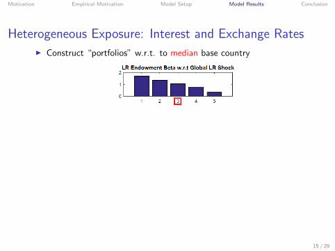
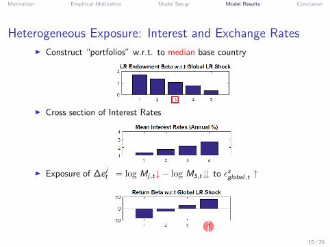
Heterogeneous Exposure: Interest and Exchange Rates
I Construct “portfolios” w.r.t. to median base country
I Cross section of Interest Rates
I Exposure of ∆e jt↑ = log Mj,t↓ − log M3,t� to εzglobal,t
15 / 29

Motivation Empirical Motivation Model Setup Model Results Conclusion
Heterogeneous Exposure: Interest and Exchange Rates
I Construct “portfolios” w.r.t. to median base country
I Cross section of Interest Rates
I Exposure of ∆e jt↑ = log Mj,t↓ − log M3,t� to εzglobal,t
15 / 29

Motivation Empirical Motivation Model Setup Model Results Conclusion
Heterogeneous Exposure: Interest and Exchange Rates
I Construct “portfolios” w.r.t. to median base country
I Cross section of Interest Rates
I Exposure of ∆e jt↑ = log Mj,t↓ − log M3,t� to εzglobal,t
15 / 29

Motivation Empirical Motivation Model Setup Model Results Conclusion
Heterogeneous Exposure: Interest and Exchange Rates
I Construct “portfolios” w.r.t. to median base country
I Cross section of Interest Rates
I Exposure of ∆e jt↑ = log Mj,t↓ − log M3,t� to εzglobal,t
15 / 29

Motivation Empirical Motivation Model Setup Model Results Conclusion
Heterogeneous Exposure: Interest and Exchange Rates
I Construct “portfolios” w.r.t. to median base country
I Cross section of Interest Rates
I Exposure of ∆e jt↑ = log Mj,t↓ − log M3,t� to εzglobal,t ↑
15 / 29
Motivation Empirical Motivation Model Setup Model Results Conclusion
Heterogeneous Exposure: Interest and Exchange Rates
I Construct “portfolios” w.r.t. to median base country
I Cross section of Interest Rates
I Exposure of ∆e jt↑ = log Mj,t↓ − log M3,t� to εzglobal,t ↑
15 / 29

Motivation Empirical Motivation Model Setup Model Results Conclusion
Heterogeneous Exposure: Interest and Exchange Rates
I Construct “portfolios” w.r.t. to median base country
I Cross section of Interest Rates
I Exposure of ∆e jt↑ = log Mj,t↓ − log M3,t� to εzglobal,t ↑
15 / 29

Motivation Empirical Motivation Model Setup Model Results Conclusion
Heterogeneous Exposure: Carry and Factor Structure
I Construct “portfolios” w.r.t. to median base country
I Carry trade returns in Model
I Lustig, Roussanov, and Verdelhan (2011) in Model
16 / 29

Motivation Empirical Motivation Model Setup Model Results Conclusion
Heterogeneous Exposure: Carry and Factor Structure
I Construct “portfolios” w.r.t. to median base country
I Carry trade returns in Model
I Lustig, Roussanov, and Verdelhan (2011) in Model
16 / 29

Motivation Empirical Motivation Model Setup Model Results Conclusion
CRRA case
I Interest Rate portfolio sorts with CRRA preferences
17 / 29

Motivation Empirical Motivation Model Setup Model Results Conclusion
NFA, FX, and Interest Rates
18 / 29

Motivation Empirical Motivation Model Setup Model Results Conclusion
Average Interest Rates and NFA
I Model: High βzi → low r if and positive NFAi
I Precautionary savings at work
19 / 29

Motivation Empirical Motivation Model Setup Model Results Conclusion
Average Interest Rates and NFA
I Model: High βzi → low r if and positive NFAi
I Precautionary savings at work
19 / 29

Motivation Empirical Motivation Model Setup Model Results Conclusion
Volatilities
I Model: High |βzi | → high σ(∆ei ) and high σ(NFAi )
I Risk sharing at work
20 / 29

Motivation Empirical Motivation Model Setup Model Results Conclusion
Conditional Responses
21 / 29

Motivation Empirical Motivation Model Setup Model Results Conclusion
Model: NFA and Exchange Rate
I Response to a positive global long-run shock
High beta Low beta
∆GDP
NFA
∆e
22 / 29

Motivation Empirical Motivation Model Setup Model Results Conclusion
Model: NFA and Exchange Rate
I Response to a positive global long-run shock
High beta Low beta
∆GDP
NFA
∆e
22 / 29

Motivation Empirical Motivation Model Setup Model Results Conclusion
Model: NFA and Exchange Rate
I Response to a positive global long-run shock
High beta Low beta
∆GDP
NFA
∆e
22 / 29

Motivation Empirical Motivation Model Setup Model Results Conclusion
Data: NFA
NFAi,t
GDPi,t= αNFA
i + λNFAi · zglobal,t + ξi,t
NZ
AUS
UK
GER
CAN
NOR
JPN
SUI
US
SWE
-700
-500
-300
-100
100
300
-0.55 -0.45 -0.35 -0.25 -0.15 -0.05 0.05 0.15 0.25 0.35
lNFA
b
23 / 29

Motivation Empirical Motivation Model Setup Model Results Conclusion
Data: NFA
NFAi,t
GDPi,t= αNFA
i + λNFAi · zglobal,t + ξi,t
NZ
AUS
UK
GER
CAN
NOR
JPN
SUI
US
SWE
-700
-500
-300
-100
100
300
-0.55 -0.45 -0.35 -0.25 -0.15 -0.05 0.05 0.15 0.25 0.35
lNFA
b
23 / 29

Motivation Empirical Motivation Model Setup Model Results Conclusion
Data: NFA
NFAi,t
GDPi,t= αNFA
i + λNFAi · zglobal,t + ξi,t
NZ
AUS
UK
GER
CAN
NOR
JPN
SUI
US
SWE
-700
-500
-300
-100
100
300
-0.55 -0.45 -0.35 -0.25 -0.15 -0.05 0.05 0.15 0.25 0.35
lNFA
b
𝑁𝐹𝐴𝑖,𝑡𝐺𝐷𝑃𝑖,𝑡
= 𝛼𝑖 + −107.31 − 609.24 ∙ 𝛽𝑖𝑧 ∙ 𝑧𝑔𝑙𝑜𝑏𝑎𝑙,𝑡
(7.42) (29.66)
24 / 29

Motivation Empirical Motivation Model Setup Model Results Conclusion
Data: Exchange Rate
∆ei,t = αFXi + λFX
i ·∆zglobal,t + ξi,t ,
NZAUS
UK GER
CAN
NOR
JPN
SUI
SWE
-135
-85
-35
15
65
-0.55 -0.45 -0.35 -0.25 -0.15 -0.05 0.05 0.15 0.25 0.35
lFX
b
25 / 29

Motivation Empirical Motivation Model Setup Model Results Conclusion
Data: Exchange Rate
∆ei,t = αFXi + λFX
i ·∆zglobal,t + ξi,t ,
NZAUS
UK GER
CAN
NOR
JPN
SUI
SWE
-135
-85
-35
15
65
-0.55 -0.45 -0.35 -0.25 -0.15 -0.05 0.05 0.15 0.25 0.35
lFX
b
25 / 29

Motivation Empirical Motivation Model Setup Model Results Conclusion
Data: Exchange Rate
∆ei,t = αFXi + λFX
i ·∆zglobal,t + ξi,t ,
NZAUS
UK GER
CAN
NOR
JPN
SUI
SWE
-135
-85
-35
15
65
-0.55 -0.45 -0.35 -0.25 -0.15 -0.05 0.05 0.15 0.25 0.35
lFX
b
∆𝑒𝑖,𝑡 = 𝛼𝑖 + −26.11 − 33.02 ∙ 𝛽𝑖𝑧 ∙ ∆𝑧𝑔𝑙𝑜𝑏𝑎𝑙,𝑡
(7.55) (11.97)
26 / 29

Motivation Empirical Motivation Model Setup Model Results Conclusion
Robustness: Currency Portfolios
I Results are robust to the exclusion of specific countries andcontrolling for local shocks
27 / 29

Motivation Empirical Motivation Model Setup Model Results Conclusion
Conclusion
28 / 29

Motivation Empirical Motivation Model Setup Model Results Conclusion
Conclusion
1. Novel empirical evidence on heterogenous exposure to global newsshocks
2. GE model with (i) recursive preferences, (ii) multiple countries, and(iii) heterogenous exposure to global news shocks
↪→ Unified framework for several phenomena.
Consistent with data, High news exposure countries have:
- Low interest rates- Safe currencies- Positive NFA positions- More volatile NFA and FX
(same for low risk exposure countries)
3. Future research: investment flows, interplay with frictions
29 / 29

Motivation Empirical Motivation Model Setup Model Results Conclusion
Conclusion
1. Novel empirical evidence on heterogenous exposure to global newsshocks
2. GE model with (i) recursive preferences, (ii) multiple countries, and(iii) heterogenous exposure to global news shocks
↪→ Unified framework for several phenomena.
Consistent with data, High news exposure countries have:
- Low interest rates
- Safe currencies- Positive NFA positions- More volatile NFA and FX
(same for low risk exposure countries)
3. Future research: investment flows, interplay with frictions
29 / 29

Motivation Empirical Motivation Model Setup Model Results Conclusion
Conclusion
1. Novel empirical evidence on heterogenous exposure to global newsshocks
2. GE model with (i) recursive preferences, (ii) multiple countries, and(iii) heterogenous exposure to global news shocks
↪→ Unified framework for several phenomena.
Consistent with data, High news exposure countries have:
- Low interest rates- Safe currencies
- Positive NFA positions- More volatile NFA and FX
(same for low risk exposure countries)
3. Future research: investment flows, interplay with frictions
29 / 29

Motivation Empirical Motivation Model Setup Model Results Conclusion
Conclusion
1. Novel empirical evidence on heterogenous exposure to global newsshocks
2. GE model with (i) recursive preferences, (ii) multiple countries, and(iii) heterogenous exposure to global news shocks
↪→ Unified framework for several phenomena.
Consistent with data, High news exposure countries have:
- Low interest rates- Safe currencies- Positive NFA positions
- More volatile NFA and FX(same for low risk exposure countries)
3. Future research: investment flows, interplay with frictions
29 / 29

Motivation Empirical Motivation Model Setup Model Results Conclusion
Conclusion
1. Novel empirical evidence on heterogenous exposure to global newsshocks
2. GE model with (i) recursive preferences, (ii) multiple countries, and(iii) heterogenous exposure to global news shocks
↪→ Unified framework for several phenomena.
Consistent with data, High news exposure countries have:
- Low interest rates- Safe currencies- Positive NFA positions- More volatile NFA and FX
(same for low risk exposure countries)
3. Future research: investment flows, interplay with frictions
29 / 29

Motivation Empirical Motivation Model Setup Model Results Conclusion
Conclusion
1. Novel empirical evidence on heterogenous exposure to global newsshocks
2. GE model with (i) recursive preferences, (ii) multiple countries, and(iii) heterogenous exposure to global news shocks
↪→ Unified framework for several phenomena.
Consistent with data, High news exposure countries have:
- Low interest rates- Safe currencies- Positive NFA positions- More volatile NFA and FX
(same for low risk exposure countries)
3. Future research: investment flows, interplay with frictions
29 / 29