cs/ee 143 communication networks chapter 5...

cs/ee 143 Communication Networks Chapter 5 Routing

Text: Walrand & Parakh, 2010

Steven Low CMS, EE, Caltech

Warning

These notes are not self-contained, probably not understandable,

unless you also were in the lecture They are supplement to not replacement for class attendance

Lecture outline

Inter-domain routing n BGP

Intra-domain routing n Shortest path algortihms

Coding n  FEC, network coding

Putting it all together 76 5. ROUTING

Figure 5.19: Figure for Routing Problem 3.

5.8 REFERENCESPeering and transit agreements are explained in (38). Dijkstra’s algorithm was published in (14).The Bellman-Ford algorithm is analyzed in (6). The QoS routing problems are studied in (41). Theoscillations of BGP are discussed in (19). BGP is described in (68). Network coding was introducedin (2) that proved the basic multicasting result. The wireless example is from (27). Packet erasurecodes are studied in (45). AODV is explained in (73) and OLSR in (74). For ant-routing, see (13).For a survey of geographic routing, see (49).

[W&P 2010] initially unconnected

What is routing?

Internet

A

B

Choose red or blue.

How to route?

Internet

A

B

Two layers of routing: 1.  Choose which AS?

- BGP 2.  How to route inside an AS?

- OSPF

Autonomy system (AS) e.g., AT&T, Verizon, MIT.

Why two layers?

o  Different objectives n  Choose AS: special policies n  Inside AS: minimize delay, # hops

o  Simplify routing n  Choose AS: ignore details inside AS n  Inside AS: only details inside AS

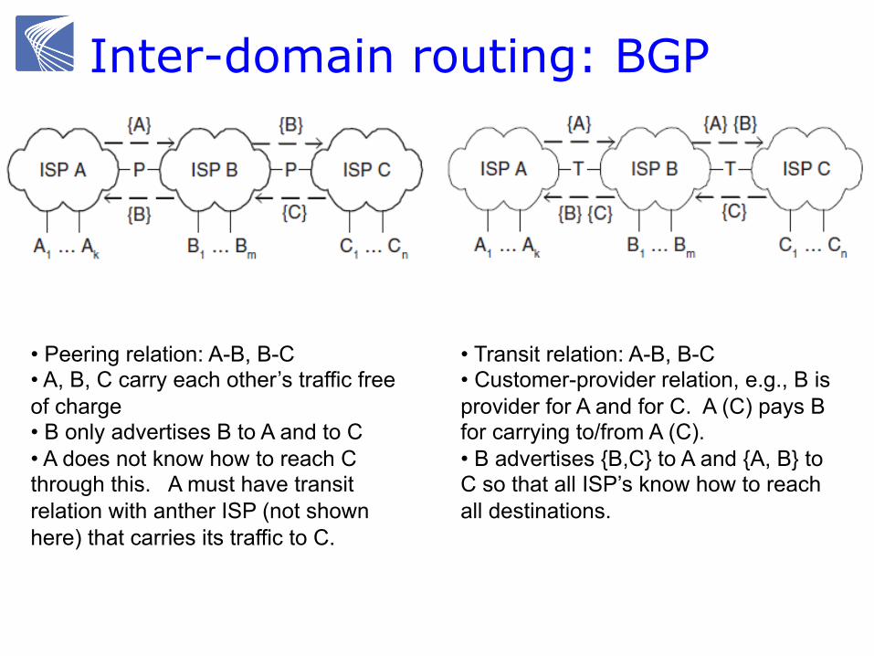
Inter-domain routing: BGP

•  Peering relation: A-B, B-C •  A, B, C carry each other’s traffic free of charge •  B only advertises B to A and to C •  A does not know how to reach C through this. A must have transit relation with anther ISP (not shown here) that carries its traffic to C.

•  Transit relation: A-B, B-C •  Customer-provider relation, e.g., B is provider for A and for C. A (C) pays B for carrying to/from A (C). •  B advertises {B,C} to A and {A, B} to C so that all ISP’s know how to reach all destinations.


A typical configuration

Inter-domain routing: BGP BGP is policy-based routing o  Generally not shortest-path o  Other factors are generally more important

in determining an AS-path than performance n  Peering agreement n  Pricing (revenue/cost) with next hop n  Reliability, security, political reasons

o  Can lead to oscillation and bad performance


Example BGP policy at Berkeley: 1.  If possible, avoid AT&T 2.  Choose path with smallest #hops 3.  Alphabetical Berkeley decision: use path Sprint-Verizon-MIT to reach MIT

Border Gateway Protocol (BGP)

How to reach MIT from Berkeley?

Every AS keeps a list of (Destination, Path) pairs & policies. Policy: avoid AT&T.

Verizon

AT&T

Sprint

Berkeley

(MIT, Verizon---MIT)

(MIT, AT&T---MIT)

(MIT, NA)

(MIT, NA)




Verizon

AT&T

Sprint

Berkeley


(MIT, AT&T---MIT)

(MIT, Sprint---Verizon---MIT)

(MIT, Berkeley---AT&T---MIT)

(MIT, Sprint---AT&T---MIT)

(MIT, Verizon---AT&T---MIT)

(MIT, AT&T---Verizon---MIT)




Verizon

AT&T

Sprint

Berkeley


(MIT, AT&T---MIT)

(MIT, Sprint---Verizon---MIT)

(MIT, Berkeley---AT&T---MIT) (MIT, Berkeley---Sprint---Verizon---MIT)

Border Gateway Protocol (BGP) In BGP, each AS o  Announces itself to other ASes and which

ASes it can reach o  Obtains ASes reachability info from

neighboring Ases o  Propagate reachability info to all routers

internal to the AS o  Determine “good” routes to ASes based on

reachability info and AS policy

BGP: potential oscillation

Example BGP policy to reach D: 1.  Prefer 2-hop path to 1-hop 2.  Avoid 3-hop paths Oscillation: Every node will alternate between choosing an 1-hop path and 2-hop path

Some questions Q1: Why not 3-level, or N-level, routing? Q2: How can a source ensure that its

packets follow the inter-domain path it wants?

Q3: In BGP, can one prevent a domain

from lying and funneling all traffic through itself in order eavesdrop?

Lecture outline




Shortest-path algorithm Input: graph ,

link costs dij ( ) Execution: algorithm run at each node Output:

n  Dijkstra: shortest-path tree rooted at the node n  Bellman-Ford: next hop to all destinations from the node

(entries in forwarding table) Notation:

n  : min cost to reach node i from x n  predx(i) : parent node of i (for Dijkstra) n  nextx(i) : next hop to i from x (for Bellman-Ford)

Ejidij ∉∞= ),( if ),( EVG =

)(iDx

Dijkstra algorithm Init: predx(i) = null Each node x sends dxi to all other nodes i

while do {

for all { if then {

pred(j) = }if }for }while

VR ≠)( minarg* iDi xRi∉

=

RiNj \)( *∈

jixx diDjD *)()( * +>

jixx diDjD *)()( * +←*i

}{ *iRR ∪←

Run at each source node x

},{,0)(,)( xRxDdiD xxix ===

Which step requires global info?

Dijkstra algorithm 5.3. INTRA-DOMAIN SHORTEST PATH ROUTING 65

B

A

F

C

ED

1

4

1 1

2

1

4

3

P(1)

1B

A

F

C

ED

1

4

1 1

2

1

4

3

P(2)

1B

A

F

C

ED

1

4

1 1

2

1

4

3

P(3)

1

2

B

A

F

C

ED

1

4

1 1

2

1

4

3

P(4)

1

2

3 B

A

F

C

ED

1

4

1 1

2

1

4

3

P(5)

1

2

3

3

B

A

F

C

ED

1

4

1 1

2

1

4

3

P(6): Final

1

2

3

3

5

Figure 5.8: Dijkstra’s routing algorithm.

To find the shortest paths from node A to all the other nodes, Dijkstra’s algorithm computesrecursively the set P(k) of the k-closest nodes to node A (shown with black nodes). The algorithmstarts with P(1) = {A}. To find P(2), it adds the closest node to the set P(1), here B, and writesits distance to A, here 1. To find P(3), the algorithm adds the closest node to P(2), here E, andwrites its distance to A, here 2. The algorithm continues in this way, breaking ties according to adeterministic rule, here favoring the lexicographic order, thus adding C before F . This is a one-passalgorithm whose number of steps is the number of nodes.

After running the algorithm, each node remembers the next step along the shortest path toeach node and stores that information in a routing table. For instance, A’s routing table specifies thatthe shortest path to E goes first along link AB. Accordingly, when A gets a packet destined to E, itsends it along link AB. Node B then forwards the packet to E.

5.3.2 BELLMAN-FORD AND DISTANCE VECTORFigure 5.9 shows the operations of a distance vector algorithm. The routers regularly send to theirneighbors their current estimate of the shortest distance to the other routers.The figure only considersdestination D, for simplicity. Initially, only node D knows that its distance to D is equal to zero, andit sends that estimate to its neighbors B and C. Router B adds the length 1 of the link BD to theestimate 0 it got from D and concludes that its estimated distance to D is 1. Similarly, C estimatesthe distance to D to be equal to 3 + 0 = 3. Routers B and C send those estimates to A. Node A

then compares the distances 2 + 1 of going to D via node B and 1 + 3 that corresponds to going toC first. Node A concludes that the estimated shortest distance to D is 3. At each step, the routers

Bellman-Ford algorithm Init: predx(i) = null Each node x sends distance vector to all its

neighbors whenever changes

do (execute when link cost changes or on receipt of a DV from neighbor) { for all destination nodes i {

nextx(i) = }for }

until no change

Dx (i) := minj∈N (x )dxj +Dj (i)( )

Run at each source node x

},{,0)(,)( xRxDdiD xxix ===

( )ViiDx ∈),(

j* := argminj∈N (i)

dxj +Dj (i)( )

( )ViiDx ∈),(

Bellman-Ford algorithm

Consider the calculations at all nodes to reach node D •  Every node has access to distance estimates from neighbors to D •  Assume synchronous operation

5.3. INTRA-DOMAIN SHORTEST PATH ROUTING 65

B

A

F

C

ED

1

4

1 1

2

1

4

3

P(1)

1B

A

F

C

ED

1

4

1 1

2

1

4

3

P(2)

1B

A

F

C

ED

1

4

1 1

2

1

4

3

P(3)

1

2

B

A

F

C

ED

1

4

1 1

2

1

4

3

P(4)

1

2

3 B

A

F

C

ED

1

4

1 1

2

1

4

3

P(5)

1

2

3

3

B

A

F

C

ED

1

4

1 1

2

1

4

3

P(6): Final

1

2

3

3

5

Figure 5.8: Dijkstra’s routing algorithm.

To find the shortest paths from node A to all the other nodes, Dijkstra’s algorithm computesrecursively the set P(k) of the k-closest nodes to node A (shown with black nodes). The algorithmstarts with P(1) = {A}. To find P(2), it adds the closest node to the set P(1), here B, and writesits distance to A, here 1. To find P(3), the algorithm adds the closest node to P(2), here E, andwrites its distance to A, here 2. The algorithm continues in this way, breaking ties according to adeterministic rule, here favoring the lexicographic order, thus adding C before F . This is a one-passalgorithm whose number of steps is the number of nodes.

After running the algorithm, each node remembers the next step along the shortest path toeach node and stores that information in a routing table. For instance, A’s routing table specifies thatthe shortest path to E goes first along link AB. Accordingly, when A gets a packet destined to E, itsends it along link AB. Node B then forwards the packet to E.

5.3.2 BELLMAN-FORD AND DISTANCE VECTORFigure 5.9 shows the operations of a distance vector algorithm. The routers regularly send to theirneighbors their current estimate of the shortest distance to the other routers.The figure only considersdestination D, for simplicity. Initially, only node D knows that its distance to D is equal to zero, andit sends that estimate to its neighbors B and C. Router B adds the length 1 of the link BD to theestimate 0 it got from D and concludes that its estimated distance to D is 1. Similarly, C estimatesthe distance to D to be equal to 3 + 0 = 3. Routers B and C send those estimates to A. Node A

then compares the distances 2 + 1 of going to D via node B and 1 + 3 that corresponds to going toC first. Node A concludes that the estimated shortest distance to D is 3. At each step, the routers

iteration

DA(D) nextA(D)

DB(D) nextB(D)

DC(D) nextC(D)

DE(D) nextE(D)

DF(D) nextF(D)

0 Inf - Inf - 2 D 4 D Inf - 1 Inf - 5 C 2  D 3  C 5 E 2 6  B 4 E 2  D 3  C 4 E 3 5  B 4  E 2  D 3  C 4 E 4 5  B 4  E 2  D 3  C 4 E

Compare Dijsktra & BF o  Message exchange

n  Dijkstra: every node sends only its incident link costs to all other nodes. This requires O(|V| |E|) messages.

n  BF: every node sends only to its neighbors least-cost estimates from itself to all other nodes

o  Speed of convergence n  Disjstra: above implementation takes O(|V|2); can be

reduced using heap n  BF: can converge slowly and have routing loops during

transient; count-to-infinity problem (can be solved using poisoned reverse)

o  No clear winner n  Both are used on Internet n  RIP: distance-vector protocol n  OSPF: link-state protocol (meant to be successor to RIP)

Count-to-infinity problem

Example Link between B & C fails A and B will not realize it, a routing route is created and their cost estimate to C keeps going up A solution: poisoned reverse: instead of telling B its true cost (2) to reach C, A tells B that its cost to reach C is infinity because A uses B to reach C.

Compare Dijsktra & BF o  Dijkstra algorithm

n  Needs global information (link-state alg) n  Each node broadcasts link-state packets to all

other nodes in network n  Each node executes Dijkstra alg to calculate

shortest paths to all other nodes n  After k iteration, shortest paths to k destinations

are known (and they are the k shortest paths among the shortest paths to all nodes)

n  Terminates after N-1 iterations (N = #nodes)

Compare Dijsktra & BF o  Bellman-Ford algorithm

n  Only needs local information (distance-vector alg) n  Each node exchanges with neighbors the vector of

distances from itself to all other nodes n  Each node then updates the next hop and

associated distance to all other nodes using Bellman-Ford (DP) equation

n  Decentralized, asynchronous, distributed

Other questions o How can routers trust each other ? o How to deal with non-convergence in

DV protocol? How often is oscillation encountered in practice?

o  Router R1 can route a pkt to host A

through R2 or R3; R2 can route through R4 or R5 and has chosen R4. But R1 prefers R5 to R2 to R4. What happens?

Other questions o What is timescale for routing update? o What are major impediments to

making significant changes to routing architecture? Would a bio-inspired routing system feasible?

o Can network coding & FEC be

combined?




[W&P 2010]

5.7. PROBLEMS 75

(a) Run Bellman-Ford algorithm on this network to compute the routing table for the nodeA. Show A’s distances to all other nodes at each step.

(b) Suppose the link A-B goes down. As a result, A advertises a distance of infinity to B.Describe in detail a scenario where C takes a long time to learn that B is no longerreachable.

P5.3 Consider the network shown below and assume the following:

• The network addresses of nodes are given by <AS>.<Network>.0.<node>, e.g., nodeA has the address AS1.E1.0.A,

• The bridge IDs satisfy B1 < B2 < B3 …,

• H is not connected to AS2.E5 for part (a),

• The BGP Speakers use the least-next-hop-cost policy for routing (i.e., among alternativepaths to the destination AS, choose the one that has the least cost on the first hop), and

• The network topology shown has been stable for a long enough time to allow all therouting algorithms to converge and all the bridges to learn where to forward each packet.

(a) What route, specified as a series of bridges and routers, would be used if G wanted tosend a packet to A?

(b) Now, if node H was added to AS2.E5, and D tried to send a packet to it as soon as H wasadded, what would happen? Specifically, will the packet reach its destination and whichall links and/or networks would the packet be sent on?

(c) Starting from the network in (b), suppose AS2.R2 goes down. Outline in brief the routingchanges that would occur as a consequence of this failure. [Hint: Think about how thechange affects packets sent from AS1 to AS2, and packets sent from AS2 to AS1.]

P5.4 Consider a wireless network with nodes X and Y exchanging packets via an access point Z.For simplicity, we assume that there are no link-layer acknowledgments. Suppose that X sendspackets to Y at rate 2R packets/sec and Y sends packets to X at rate R pacekts/sec; all thepackets are of the maximum size allowed. The access point uses network coding. That is,whenever it can, it sends the "exclusive or" of a packet from X and a packet from Y instead ofsending the two packets separately.

(a) What is the total rate of packet transmissions by the three nodes without network coding?

(b) What is the total rate of packet transmissions by the three nodes with network coding?





1.  How to route G à A? 2.  As soon as H is added, D tries to send a packet to H. What happens? 3.  If AS2.R2 goes down, what will be the routing changes?

later goes down

1. compute spanning tree 76 5. ROUTING



[W&P 2010]

2. compute intra-AS routing 76 5. ROUTING



[W&P 2010]

3. compute inter-AS routing 76 5. ROUTING



[W&P 2010]

1.  How to route G à A?

3. compute inter-AS routing 76 5. ROUTING



[W&P 2010]

1.  How to route G à A? Does A à G follow the same path?

4. Address resolution protocol 76 5. ROUTING



[W&P 2010]


initially unconnected

4. Address resolution protocol 76 5. ROUTING



[W&P 2010]

•  Packets from D can be delivered to subnet AS2.B1 based on IP address of H •  AS2.B1 does not know H •  AS2.B1 uses ARP to find H’s MAC address •  Use STP to forward pkts to H

initially unconnected

Example: H1 wants to send packet to H2

Ethernet switch

gateway

Link

Network

[all, e1, who is IP2?]

Link layer on H1 broadcasts a message (ARP query) on its layer 2 network asking for the MAC address corresponding to IP2


Ethernet switch

gateway

Link

Network

[all, e1, who is IP2?]

Link

Network

[e1, e2, I am IP2]

Link layer on H2 responds to the ARP query with its MAC address


Ethernet switch

gateway

Link

Network

Link

Network

Once the link layer on H1 knows e2, it can now send the original message

[e2, e1,[IP1, IP2, X]]


Ethernet switch

gateway

Link

Network

Link

Network

Link layer on H2 delivers the packet to the network layer on H2

[e2, e1,[IP1, IP2, X]]

[IP1, IP2, X]

[e2, e1,[IP1, IP2, X]]

5. re-compute routing table 76 5. ROUTING



[W&P 2010]


goes down

5. re-compute routing tables 76 5. ROUTING



[W&P 2010]

goes down

•  Failure detected by AS2.R1 and AS2.R3; update routing tables (intra-AS) •  Failure detected by border gateway in AS5 •  BGP re-computes •  The path between AS2 and AS5 will be changed

Lecture outline




FEC: packet erasure code

Recover from packet loss Coding

n  Input: n packets n  Output: m packets

o  = bit-by-bit XOR of a random subset of

o  Header of specifies the subset used to generate

Ck := Pi1 ⊕ Pi2 ⊕⊕ Pijk

P1,,PnC1,,Cm, m > n

CkP1,,Pn{ }

Ck Ck

FEC: packet erasure code

Decoding n  If for some i, then for all pkts that contains n  Remove from the collection of rec’d pkts n  Repeat until all have been decoded n  If at one step, there is no

then decoding fails Cj ∈ P1,,Pn{ }

Cj = PiCk :=Ck ⊕ Pi Ck Pi

Cj

P1,,Pn

FEC: example

C = C1,C3,C5,C6{ }

C1 = P1 C3 = P1⊕ P2 ⊕ P3

5.4. ANYCAST, MULTICAST 69

it can connect to that tree. This is less optimal than a Steiner tree from oakland, but the algorithmis much less complex.

5.4.3 FORWARD ERROR CORRECTIONUsing retransmissions to make multicast reliable is not practical. Imagine multicasting a file or avideo stream to 1000 users. If one packet gets lost on a link of the multicast tree, hundreds of usersmay miss that packet. It is not practical for them all to send a negative acknowledgment. It is notfeasible either for the source to keep track of positive acknowledgments from all the users.

A simpler method is to add additional packets to make the transmission reliable.This schemeis called a packet erasure code because it is designed to be able to recover from ‘erasures" of packets,that is, from packets being lost in the network. For instance, say that you want to send packets P 1and P 2 of 1KByte to a user, but that it is likely that one of the two packets could get lost.To improvereliability, one can send {P 1, P 2, C} where C is the addition bit by bit, modulo 2, of the packets P 1and P 2. If the user gets any two of the packets {P 1, P 2, C}, it can recover the packets P 1 and P 2.For instance, if the user gets P 1 and C, it can reconstruct packet P2 by adding P 1 and C bit by bit,modulo 2.

This idea extends to n packets {P 1, P 2, . . . , Pn} as follows: one calculates each of the pack-ets {C1, C2, . . . , Cm} as the sum bit by bit modulo 2 of a randomly selected set of packets in{P 1, P 2, . . . , Pn}. The header of packet Ck specifies the subset of {1, 2, . . . , n} that was used tocalculate Ck. If m is sufficiently large, one can recover the original packets from any n of the packets{C1, C2, . . . , Cm}.

One decoding algorithm is very simple. It proceeds as follows:

• If one of the Ck, say Cj , is equal to one of the packets {P 1, . . . , Pn}, say P i, then P i has beenrecovered. One then adds P i to all the packets Cr that used that packet in their calculation.

• One removes the packet Cj from the collection and one repeats the procedure.

• If at one step one does not find a packet Cj that involves only one P i, the procedure fails.

P1 P2 P3 P4

C1 C2 C3 C4 C5 C6 C7

Figure 5.13: Calculation of FEC packets.

: received pkt

Decoding: received pkts

C5 = P4 C6 = P3 ⊕ P4

C3←C3 ⊕C1 = P2 ⊕ P3

C = C3,C5,C6{ } P← P1{ }

P = { }C = C1,C3,C5,C6{ }

FEC: example

C1 = P1 C3 = P1⊕ P2 ⊕ P3










P1 P2 P3 P4

C1 C2 C3 C4 C5 C6 C7


: received pkt

Decoding:

C5 = P4 C6 = P3 ⊕ P4

C3←C3 ⊕C1 = P2 ⊕ P3

C = C3,C5,C6{ } P← P1{ }

P = { }C = C1,C3,C5,C6{ }

FEC: example

C3 = P2 ⊕ P3










P1 P2 P3 P4

C1 C2 C3 C4 C5 C6 C7


: received pkt

Decoding:

C5 = P4 C6 = P3 ⊕ P4

C6 ←C6 ⊕C5 = P3

C = C3,C6{ } P← P1,P4{ }

P = P1{ }C = C3,C5,C6{ }

FEC: example

C3 = P2 ⊕ P3










P1 P2 P3 P4

C1 C2 C3 C4 C5 C6 C7


: received pkt

Decoding:

C6 = P3

C3←C3 ⊕C6 = P2

C = C6{ } P← P1,P3,P4{ }

P = P1,P4{ }C = C3,C6{ }

FEC: example

C3 = P2 ⊕ P3










P1 P2 P3 P4

C1 C2 C3 C4 C5 C6 C7


: received pkt

Decoding:

C6 = P3

C3←C3 ⊕C6 = P2

C = C3{ } P← P1,P3,P4{ }

P = P1,P4{ }C = C3,C6{ }

FEC: example

C3 = P3










P1 P2 P3 P4

C1 C2 C3 C4 C5 C6 C7


: received pkt

Decoding:

C = { } P← P1,P2,P3,P4{ }

P = P1,P2,P4{ }C = C3{ }

Network coding: example


S

T UW

XY Z

X

S

T UW

XY Z

X

b1 b2b1 b2

b1 b1b1

b1

b2

b1 b2b1 b2

b1b1�b2

b2b1�b2

b1�b2

Figure 5.15: Multicast from S to X and Y without (left) and with (right) network coding.

in the right part of the figure, the network can deliver packets at the rate of 2R to both Y and Z.Without network coding, as shown on the left, the network can only deliver one bit to Y and two bitsto Z (or, two bits to Y and one bit to Z). One can show that the network can achieve a throughputof 1.5R to both Y and Z without network coding.

The general result about network coding and multicasting is as follows. Consider a generalnetwork and assume that the feasible rate from S to any one node in N is at least R. Then, usingnetwork coding, it is possible to multicast the packets from S to N at rate R. For instance, in thenetwork of Figure 5.15, the rate from S to Y is equal to 2R as we can see by considering the twodisjoint paths ST Y and SUWXY . Similarly, the rate from S to Z is also 2R.Thus, one can multicastpackets from S to Y and Z at rate 2R.

Network coding can also be useful in wireless networks, as the following simple exampleshows. Consider the network in Figure 5.16.There are two WiFi clients X and Y that communicatevia access point Z. Assume that X needs to send packet A to Y and that Y needs to send packet B

to X.

A B

A � B A � B

(1) (2)

(3)

X YZ

Figure 5.16: Network coding for a WiFi network.

The normal procedure for X and Y to exchange A and B requires transmitting four packetsover the wireless channel: packet A from X to Z, packet A from Z to Y , packet B from Y to Z,and packet B from Z to X. Using network coding, the devices transmit only three packets: packet

•  link rate = R on every link •  multicast to both Y & Z

throughput = 1.5R throughput = 2R


S

T UW

XY Z

X

S

T UW

XY Z

X

b1 b2b1 b2

b1 b1b1

b1

b2

b1 b2b1 b2

b1b1�b2

b2b1�b2

b1�b2

Figure 5.15: Multicast from S to X and Y without (left) and with (right) network coding.

in the right part of the figure, the network can deliver packets at the rate of 2R to both Y and Z.Without network coding, as shown on the left, the network can only deliver one bit to Y and two bitsto Z (or, two bits to Y and one bit to Z). One can show that the network can achieve a throughputof 1.5R to both Y and Z without network coding.

The general result about network coding and multicasting is as follows. Consider a generalnetwork and assume that the feasible rate from S to any one node in N is at least R. Then, usingnetwork coding, it is possible to multicast the packets from S to N at rate R. For instance, in thenetwork of Figure 5.15, the rate from S to Y is equal to 2R as we can see by considering the twodisjoint paths ST Y and SUWXY . Similarly, the rate from S to Z is also 2R.Thus, one can multicastpackets from S to Y and Z at rate 2R.

Network coding can also be useful in wireless networks, as the following simple exampleshows. Consider the network in Figure 5.16.There are two WiFi clients X and Y that communicatevia access point Z. Assume that X needs to send packet A to Y and that Y needs to send packet B

to X.

A B

A � B A � B

(1) (2)

(3)

X YZ

Figure 5.16: Network coding for a WiFi network.

The normal procedure for X and Y to exchange A and B requires transmitting four packetsover the wireless channel: packet A from X to Z, packet A from Z to Y , packet B from Y to Z,and packet B from Z to X. Using network coding, the devices transmit only three packets: packet

Network coding: example

X and Y want to exchange A & B

•  Without network coding, needs 4 pkt xmissions •  With network coding, needs 3 pkt xmissions

cs/ee 143 communication networks chapter 5...

Documents