CSE 613: Parallel Programming

Lecture 6

( High Probability Bounds )

Rezaul A. Chowdhury

Department of Computer Science

SUNY Stony Brook

Spring 2012

Markov’s Inequality

Theorem 1: Let �be a random variable that assumes only

nonnegative values. Then for all � � 0,

Pr � � � �� .

Proof: For � � 0, let

� �1if� � �;0otherwise.

Since � � 0, � ��.

We also have, � Pr � 1 Pr � � � .

Then Pr � � � � �� � �

� .

Example: Coin Flipping

Let us bound the probability of obtaining more than ��� heads in a

sequence of � fair coin flips.

Let

� �1ifthe!thcoinflipisheads;0otherwise.

Then the number of heads in � flips, � ∑ � � )* .

We know, � Pr � 1 *+.

Hence, � ∑ � �+

� )* .

Then applying Markov’s inequality,

Pr � � ��� � �

�� �⁄ � +⁄�� �⁄ +

�.

Chebyshev’s Inequality

Theorem 2: For any � � 0,

Pr � - � � � ./0 ��+ .

Proof: Observe that Pr � - � � � Pr � - � + � �+ .

Since � - � + is a nonnegative random variable, we can use

Markov’s inequality,

Pr � - � + � �+ � �1� � 2�2 345 �

�2 .

Example: 6 Fair Coin Flips

� �1ifthe!thcoinflipisheads;0otherwise.

Then the number of heads in � flips, � ∑ � � )* .

We know, � Pr � 1 *+ and � + � *

+.

Then ./0 � � + - � + *+ - *

� *�.

Hence, � ∑ � �+

� )* and ./0 � ∑ ./0 � ��

� )* .

Then applying Chebyshev’s inequality,

Pr � � ��� Pr � - � � �

� 345 �� �⁄ 2 � �⁄

� �⁄ 2 ��.

Preparing for Chernoff Bounds

Lemma 1: Let �*, … , �� be independent Poisson trials, that is, each

� is a 0-1 random variable with Pr � 1 9 for some 9 . Let

� ∑ � � )* and : � . Then for any ; � 0,

<=� < >?1* @.Proof: <=�A 9 <=B* C 1 - 9 <=BD 9 <= C 1 - 9

1 C 9 <= - 1But for any E, 1 C E <F. Hence, <=�A <GA >?1* .

Now, <=� <= ∑ �AHAIJ ∏ <=�A� )* ∏ <=�A� )*

L <GA >?1*�

)* < >?1* ∑ GAHAIJ

But, : � ∑ � � )* ∑ � ∑ 9 � )* .� )*Hence, <=� < >?1* @.

Chernoff Bound 1

Theorem 3: Let �*, … , �� be independent Poisson trials, that is,

each � is a 0-1 random variable with Pr � 1 9 for some 9 . Let � ∑ � � )* and : � . Then for any � � 0,

Pr � � 1 C � : >M*N� JOM

@.

Proof: Applying Markov’s inequality for any ; � 0,

Pr � � 1 C � : Pr <=� � <= *N� @ <=�

<= *N� @

> P?QJ R>? JOM R [ Lemma 1 ]

Setting ; ln 1 C � � 0, i.e., <= 1 C �, we get,

Pr � � 1 C � : >M*N� JOM

@.

Chernoff Bound 2

Theorem 4: For 0 S � S 1, Pr � � 1 C � : <1RM2T .

Proof: From Theorem 3, for � � 0, Pr � � 1 C � : >M*N� JOM

@.

We will show that for 0 S � S 1, >M

*N� JOM <1M2T

⇒� - 1 C � ln 1 C � - �2�

That is, U � � - 1 C � ln 1 C � C �2� 0

We have, U′ � - ln 1 C � C +� �,and U′′ � - *

*N� C +�

Observe that U′′ � S 0 for 0 � *+ , and U′′ � � 0 for � � *

+ .

Chernoff Bound 2

Theorem 4: For 0 S � S 1, Pr � � 1 C � : <1RM2T .

Proof: From Theorem 3, for � � 0, Pr � � 1 C � : >M*N� JOM

@.

We will show that for 0 S � S 1, >M

*N� JOM <1M2T

⇒� - 1 C � ln 1 C � - �2�

That is, U � � - 1 C � ln 1 C � C �2� 0

We have, U′ � - ln 1 C � C +� �,and U′′ � - *

*N� C +�

Observe that U′′ � S 0 for 0 � *+ , and U′′ � � 0 for � � *

+ .

Chernoff Bound 2

Theorem 4: For 0 S � S 1, Pr � � 1 C � : <1RM2T .

Proof: From Theorem 3, for � � 0, Pr � � 1 C � : >M*N� JOM

@.

We will show that for 0 S � S 1, >M

*N� JOM <1M2T

⇒� - 1 C � ln 1 C � - �2�

That is, U � � - 1 C � ln 1 C � C �2� 0

We have, U′ � - ln 1 C � C +� �,and U′′ � - *

*N� C +�

Observe that U′′ � S 0 for 0 � *+ , and U′′ � � 0 for � � *

+ .

Hence, UW � first decreases and then increases over 0,1 .

Since UW 0 0 and UW 1 S 0, we have UW � 0 over 0,1 .

Chernoff Bound 2

Theorem 4: For 0 S � S 1, Pr � � 1 C � : <1RM2T .

Proof: From Theorem 3, for � � 0, Pr � � 1 C � : >M*N� JOM

@.

We will show that for 0 S � S 1, >M

*N� JOM <1M2T

⇒� - 1 C � ln 1 C � - �2�

That is, U � � - 1 C � ln 1 C � C �2� 0

We have, U′ � - ln 1 C � C +� �,and U′′ � - *

*N� C +�

Observe that U′′ � S 0 for 0 � *+ , and U′′ � � 0 for � � *

+ .

Hence, UW � first decreases and then increases over 0,1 .

Since UW 0 0 and UW 1 S 0, we have UW � 0 over 0,1 .

Chernoff Bound 2

Theorem 4: For 0 S � S 1, Pr � � 1 C � : <1RM2T .

Proof: From Theorem 3, for � � 0, Pr � � 1 C � : >M*N� JOM

@.

We will show that for 0 S � S 1, >M

*N� JOM <1M2T

⇒� - 1 C � ln 1 C � - �2�

That is, U � � - 1 C � ln 1 C � C �2� 0

We have, U′ � - ln 1 C � C +� �,and U′′ � - *

*N� C +�

Observe that U′′ � S 0 for 0 � *+ , and U′′ � � 0 for � � *

+ .

Hence, UW � first decreases and then increases over 0,1 .

Since UW 0 0 and UW 1 S 0, we have UW � 0 over 0,1 .

Since U 0 0, it follows that U � 0 in that interval.

Chernoff Bound 2

Theorem 4: For 0 S � S 1, Pr � � 1 C � : <1RM2T .

Proof: From Theorem 3, for � � 0, Pr � � 1 C � : >M*N� JOM

@.

We will show that for 0 S � S 1, >M

*N� JOM <1M2T

⇒� - 1 C � ln 1 C � - �2�

That is, U � � - 1 C � ln 1 C � C �2� 0

We have, U′ � - ln 1 C � C +� �,and U′′ � - *

*N� C +�

Observe that U′′ � S 0 for 0 � *+ , and U′′ � � 0 for � � *

+ .

Hence, UW � first decreases and then increases over 0,1 .

Since UW 0 0 and UW 1 S 0, we have UW � 0 over 0,1 .

Since U 0 0, it follows that U � 0 in that interval.

Chernoff Bound 2

Theorem 4: For 0 S � S 1, Pr � � 1 C � : <1RM2T .

Proof: From Theorem 3, for � � 0, Pr � � 1 C � : >M*N� JOM

@.

We will show that for 0 S � S 1, >M

*N� JOM <1M2T

⇒� - 1 C � ln 1 C � - �2�

That is, U � � - 1 C � ln 1 C � C �2� 0

We have, U′ � - ln 1 C � C +� �,and U′′ � - *

*N� C +�

Observe that U′′ � S 0 for 0 � *+ , and U′′ � � 0 for � � *

+ .

Hence, UW � first decreases and then increases over 0,1 .

Since UW 0 0 and UW 1 S 0, we have UW � 0 over 0,1 .

Since U 0 0, it follows that U � 0 in that interval.

Chernoff Bound 3

Corollary 1: For 0 S X S :,Pr � � : C X <1Y2TR .

Proof: From Theorem 2, for 0 S � S 1, Pr � � 1 C � : S <1RM2T .

Setting X :�, we get, Pr � � : C X <1Y2TR for 0 S X S :.

Example: 6 Fair Coin Flips

� �1ifthe!thcoinflipisheads;0otherwise.

Then the number of heads in � flips, � ∑ � � )* .

We know, � Pr � 1 *+.

Hence, : � ∑ � �+

� )* .

Now putting � *+ in Chernoff bound 2, we have,

Pr � � ��� <1 H

2Z *>

H2Z

.

Chernoff Bounds 4, 5 and 6

Corollary 2: For 0 S X S :,Pr � : - X <1Y22R .

Theorem 5: For 0 S � S 1, Pr � 1 - � : >QM*1� JQM

@.

Theorem 6: For 0 S � S 1, Pr � 1 - � : <1RM22 .

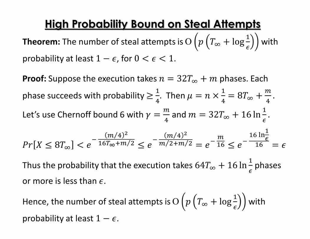
High Probability Bound on Steal Attempts

Theorem: The number of steal attempts is Ο 9 [\ C log *^ with

probability at least 1 - _, for 0 S _ S 1.

Proof: Suppose the execution takes � 32[\ C b phases. Each

phase succeeds with probability � *�. Then : � B *

� 8[\ C d� .

Let’s use Chernoff bound 6 with X d� and b 32[\ C 16 ln *

^ .

f0 � 8[\ S <1 d �⁄ 2*ghiNd +⁄ <1 d �⁄ 2

d +⁄ Nd +⁄ <1d*g <1*g jk*^*g _

Thus the probability that the execution takes 64[\ C 16 ln *^ phases

or more is less than _.

Hence, the number of steal attempts is Ο 9 [\ C log *^ with

probability at least 1 - _.

Parallel Sample Sort

Task: Sort an array m 1,… , � of � distinct keys using 9 � processors.

Steps:

1. Pivot Selection: Select and sort b 9 - 1 pivot elements <*, <+, … , <d.

These elements define b C 1 9 buckets:

-∞, <* , <*, <+ , … , <d1*, <d , <d, C∞2. Local Sort: Divide m into 9 segments of equal size, assign each segment

to different processor, and sort locally.

3. Local Bucketing: Each processor inserts the pivot elements into its local

sorted sequence using binary search, and thus divide the keys among

b C 1 9 buckets.

4. Merge Local Buckets: Processor ! 1 ! 9 merges the contents of

bucket !from all processors through a local sort.

5. Final Result: Each processor copies its bucket to a global output array so

that bucket ! 1 ! 9 - 1 precedes bucket ! C 1 in the output.

Pivot Selection & Load Balancing

In step 4 of the algorithm each processor works on a different bucket.

If bucket sizes are not reasonably uniform some processors may

become overloaded while some others may mostly sit idle in that step.

We need to select the pivot elements carefully so that the bucket sizes

are as balanced as possible.

We may choose the b 9 - 1 pivots uniformly at random so that the

expected size of a bucket is �d.

But if we use such a scheme the largest bucket can still have �d logb

keys with significant probability leading to significant load imbalance.

A better approach is to use oversampling.

Oversampling for Pivot Selection

Steps:

1. Pivot Selection:

a) For some oversampling factor o, select ob keys uniformly at random.

Each processor can choose pdG keys in parallel.

b) Sort the selected keys on a single processor.

c) Select the every o-th key as a pivot from the sorted sequence.

Bound on Bucket Sizes

Proof: Split the sorted sequence of � keys into d+ blocks of size

+�d each.

Since every o-th sample is retained as a pivot, at least one pivot will be

chosen from a block provided at least o C 1 samples are drawn from it.

Fix a block. Let random variable � be 1 if the !-th key of the block is

sampled, and 0 otherwise. All � ‘s are independent. Let � ∑ � � )* .

Then : � ∑ � +� d⁄ )* ∑ � +�

d+� d⁄ )* B pd

� 2o.

Theorem: If ob keys are initially sampled then no bucket will contain

more than ��d keys with probability at least 1 - *

�2, provided o 12 ln �.

Proof ( continued ): Now putting � *+ in Chernoff bound 5, we get,

Pr � S o C 1 Pr � o Pr � 1 - 12 : <1@

+*+

2 <1p

�.

For o 12 ln �, Pr � S o C 1 <1qZ <1� jk � *

�T.

Hence, Pr ;r<0<!o/stuvwx!;ruy;/9!zu; d+ ∙ *

�T *�2.

Thus, Pr �ustuvwx!;ruy;/9!zu; � 1 - *�2.

Size of a bucket in that case S 2 B +�d ��

d .

Theorem: If ob keys are initially sampled then no bucket will contain

more than ��d keys with probability at least 1 - *

�2, provided o 12 ln �.

Bound on Bucket Sizes

Parallel Running Time of Parallel Sample Sort

Steps:

1. Pivot Selection:

a) ΟpdG Ο log � [ worst case ]

b) Ο ob log ob Ο 9 log2 � [ worst case ]

c) Ο b Ο 9 [ worst case ]

2. Local Sort: Ο�G log �

G [ worst case ]

3. Local Bucketing: Ο b log �G Ο 9 log �

G [ worst case ]

4. Merge Local Buckets: ��d log ��

d Ο�G log �

G [ w.h.p. ]

5. Final Result: Ο��d Ο

�G [ w.h.p. ]

Overall: Ο�G log �

G C 9 log2 � [ w.h.p. ]