cse 258 lecture 8 - home | computer science and...
TRANSCRIPT

CSE 258 – Lecture 8Web Mining and Recommender Systems
Extensions of latent-factor models,
(and more on the Netflix prize!)
Summary so far
Recap
1. Measuring similarity between users/items for
binary prediction
Jaccard similarity
2. Measuring similarity between users/items for real-
valued prediction
cosine/Pearson similarity
3. Dimensionality reduction for real-valued prediction
latent-factor models

Monday…
In 2006, Netflix created a dataset of 100,000,000 movie ratings
Data looked like:
The goal was to reduce the (R)MSE at predicting ratings:
Whoever first manages to reduce the RMSE by 10% versus
Netflix’s solution wins $1,000,000
model’s prediction ground-truth

Monday…
Let’s start with the
simplest possible model:
user item

Monday…
What about the 2nd simplest model?
user item
how much does
this user tend to
rate things above
the mean?
does this item tend
to receive higher
ratings than others
e.g.

Latent-factor models
my (user’s)
“preferences”HP’s (item)
“properties”
Let’s write this as:

Latent-factor models
This gives rise to a simple (though
approximate) solution
1) fix . Solve
2) fix . Solve
3,4,5…) repeat until convergence
objective:
Each of these subproblems is “easy” – just regularized
least-squares, like we’ve been doing since week 1. This
procedure is called alternating least squares.

Latent-factor models
Movie features: genre,
actors, rating, length, etc.
User features:
age, gender,
location, etc.
Observation: we went from a method
which uses only features:
to one which completely ignores them:

Latent-factor models
Should we use features or not?
1) Argument against features:Imagine incorporating features into the model like:
which is equivalent to:
knowns unknowns
but this has fewer degrees of freedom than a
model which replaces the knowns by unknowns:

Latent-factor models
Should we use features or not?
1) Argument against features:
So, the addition of features adds no expressive power to the
model. We could have a feature like “is this an action
movie?”, but if this feature were useful, the model would
“discover” a latent dimension corresponding to action
movies, and we wouldn’t need the feature anyway
In the limit, this argument is valid: as we add more ratings
per user, and more ratings per item, the latent-factor model
should automatically discover any useful dimensions of
variation, so the influence of observed features will disappear

Latent-factor models
Should we use features or not?
2) Argument for features:
But! Sometimes we don’t have many ratings per user/item
Latent-factor models are next-to-useless if either the user or
the item was never observed before
reverts to zero if we’ve never seen the user before
(because of the regularizer)

Latent-factor models
Should we use features or not?
2) Argument for features:
This is known as the cold-start problem in recommender
systems. Features are not useful if we have many
observations about users/items, but are useful for new users
and items.
We also need some way to handle users who are active, but
don’t necessarily rate anything, e.g. through implicit
feedback

Overview & recap
So far we’ve followed the
programme below:
1. Measuring similarity between users/items for
binary prediction (e.g. Jaccard similarity)
2. Measuring similarity between users/items for real-
valued prediction (e.g. cosine/Pearson similarity)
3. Dimensionality reduction for real-valued
prediction (latent-factor models)
4. Finally – dimensionality reduction for binary
prediction

One-class recommendation
How can we use dimensionality
reduction to predict binary
outcomes?
• In weeks 1&2 we saw regression and logistic
regression. These two approaches use the same
type of linear function to predict real-valued and
binary outputs
• We can apply an analogous approach to binary
recommendation tasks

One-class recommendation
This is referred to as “one-class”
recommendation
• In weeks 1&2 we saw regression and logistic
regression. These two approaches use the same
type of linear function to predict real-valued and
binary outputs
• We can apply an analogous approach to binary
recommendation tasks
One-class recommendation
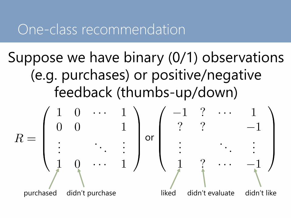
Suppose we have binary (0/1) observations
(e.g. purchases) or positive/negative
feedback (thumbs-up/down)
or
purchased didn’t purchase liked didn’t evaluate didn’t like

One-class recommendation
So far, we’ve been fitting functions of the
form
• Let’s change this so that we maximize the difference in
predictions between positive and negative items
• E.g. for a user who likes an item i and dislikes an item j we
want to maximize:

One-class recommendation
We can think of this as maximizing the
probability of correctly predicting pairwise
preferences, i.e.,
• As with logistic regression, we can now maximize the
likelihood associated with such a model by gradient ascent
• In practice it isn’t feasible to consider all pairs of
positive/negative items, so we proceed by stochastic gradient
ascent – i.e., randomly sample a (positive, negative) pair and
update the model according to the gradient w.r.t. that pair

One-class recommendation

Summary
Recap
1. Measuring similarity between users/items for
binary prediction
Jaccard similarity
2. Measuring similarity between users/items for real-
valued prediction
cosine/Pearson similarity
3. Dimensionality reduction for real-valued prediction
latent-factor models
4. Dimensionality reduction for binary prediction
one-class recommender systems

Questions?
Further reading:One-class recommendation:
http://goo.gl/08Rh59
Amazon’s solution to collaborative filtering at scale:
http://www.cs.umd.edu/~samir/498/Amazon-Recommendations.pdfAn (expensive) textbook about recommender systems:
http://www.springer.com/computer/ai/book/978-0-387-85819-7
Cold-start recommendation (e.g.):
http://wanlab.poly.edu/recsys12/recsys/p115.pdf

CSE 258 – Lecture 8Web Mining and Recommender Systems
Extensions of latent-factor models,
(and more on the Netflix prize!)

Extensions of latent-factor models
So far we have a model that looks like:
How might we extend this to:• Incorporate features about users and items
• Handle implicit feedback
• Change over time
See Yehuda Koren (+Bell & Volinsky)’s magazine article:
“Matrix Factorization Techniques for Recommender Systems”
IEEE Computer, 2009

Extensions of latent-factor models
1) Features about users and/or items
(simplest case) Suppose we have binary attributes to
describe users or items
A(u) = [1,0,1,1,0,0,0,0,0,1,0,1]
attribute vector for user u
e.g. is female is male is between 18-24yo
Extensions of latent-factor models
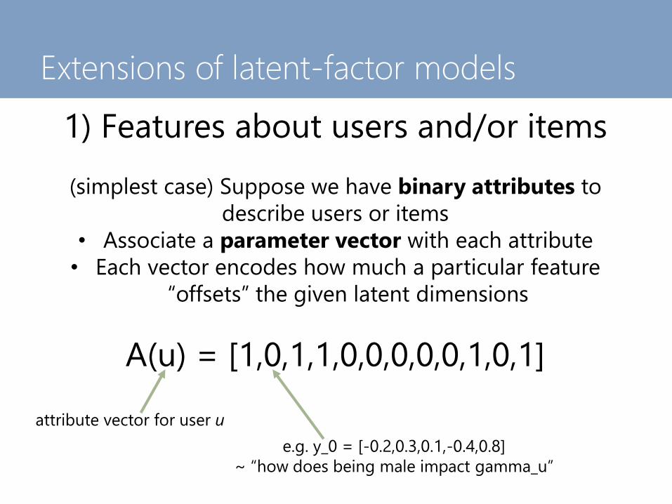
1) Features about users and/or items
(simplest case) Suppose we have binary attributes to
describe users or items
• Associate a parameter vector with each attribute
• Each vector encodes how much a particular feature
“offsets” the given latent dimensions
A(u) = [1,0,1,1,0,0,0,0,0,1,0,1]
attribute vector for user u
e.g. y_0 = [-0.2,0.3,0.1,-0.4,0.8]
~ “how does being male impact gamma_u”

Extensions of latent-factor models
1) Features about users and/or items
(simplest case) Suppose we have binary attributes to
describe users or items
• Associate a parameter vector with each attribute
• Each vector encodes how much a particular feature
“offsets” the given latent dimensions
• Model looks like:
• Fit as usual:
error regularizer

Extensions of latent-factor models
2) Implicit feedback
Perhaps many users will never actually rate things, but may
still interact with the system, e.g. through the movies they
view, or the products they purchase (but never rate)
• Adopt a similar approach – introduce a binary vector
describing a user’s actions
N(u) = [1,0,0,0,1,0,….,0,1]
implicit feedback vector for user u
e.g. y_0 = [-0.1,0.2,0.3,-0.1,0.5]
Clicked on “Love Actually” but didn’t watch

Extensions of latent-factor models
2) Implicit feedback
Perhaps many users will never actually rate things, but may
still interact with the system, e.g. through the movies they
view, or the products they purchase (but never rate)
• Adopt a similar approach – introduce a binary vector
describing a user’s actions
• Model looks like:
normalize by the number of actions the user performed

Extensions of latent-factor models
3) Change over time
There are a number of reasons why rating data might be
subject to temporal effects…

Extensions of latent-factor models
3) Change over time
Netflix ratings
over time
early 2004
Figure from Koren: “Collaborative Filtering with Temporal Dynamics” (KDD 2009)
Netflix changed
their interface!

Extensions of latent-factor models
3) Change over time
Netflix ratings by
movie age
Figure from Koren: “Collaborative Filtering with Temporal Dynamics” (KDD 2009)
People tend to give higher
ratings to older movies

Extensions of latent-factor models
3) Change over time
A few temporal effects from beer reviews

Extensions of latent-factor models
3) Change over time
There are a number of reasons why rating data might be
subject to temporal effects…
e.g. “Collaborative filtering
with temporal dynamics”
Koren, 2009
• Changes in the interface
• People give higher ratings to older movies (or, people
who watch older movies are a biased sample)
• The community’s preferences gradually change over time
• My girlfriend starts using my Netflix account one day
• I binge watch all 144 episodes of buffy one week and
then revert to my normal behavior
• I become a “connoisseur” of a certain type of movie
• Anchoring, public perception, seasonal effects, etc.
e.g. “Sequential & temporal
dynamics of online opinion”
Godes & Silva, 2012
e.g. “Temporal
recommendation on graphs
via long- and short-term
preference fusion”
Xiang et al., 2010
e.g. “Modeling the evolution
of user expertise through
online reviews”
McAuley & Leskovec, 2013

Extensions of latent-factor models
3) Change over time
Each definition of temporal evolution demands a slightly
different model assumption (we’ll see some in more detail
later tonight!) but the basic idea is the following:
1) Start with our original model:
2) And define some of the parameters as a function of time:
3) Add a regularizer to constrain the time-varying terms:
parameters should change smoothly

Extensions of latent-factor models
3) Change over time
Later: how do people acquire tastes for beers (and
potentially for other things) over time?
Differences between
“beginner” and “expert”
preferences for different
beer styles

Extensions of latent-factor models
4) Missing-not-at-random
• Our decision about whether to purchase a movie (or
item etc.) is a function of how we expect to rate it
• Even for items we’ve purchased, our decision to enter a
rating or write a review is a function of our rating
• e.g. some rating distribution from a few datasets:
EachMovie MovieLens Netflix
Figure from Marlin et al. “Collaborative Filtering and the Missing at Random Assumption” (UAI 2007)

Extensions of latent-factor models
4) Missing-not-at-random
e.g. Men’s watches:

Extensions of latent-factor models
4) Missing-not-at-random
• Our decision about whether to purchase a movie (or
item etc.) is a function of how we expect to rate it
• Even for items we’ve purchased, our decision to enter a
rating or write a review is a function of our rating
• So we can predict ratings more accurately by building
models that account for these differences
1. Not-purchased items have a different prior on ratings
than purchased ones
2. Purchased-but-not-rated items have a different prior on
ratings than rated ones
Figure from Marlin et al. “Collaborative Filtering and the Missing at Random Assumption” (UAI 2007)
Moral(s) of the story
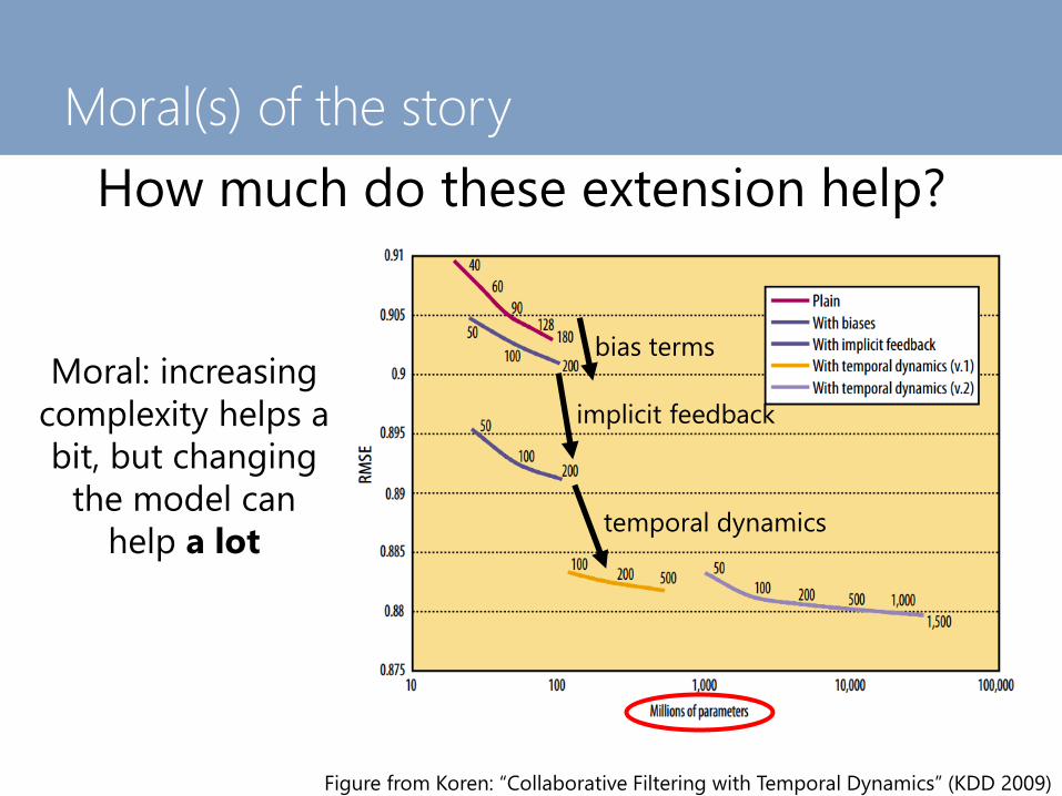
How much do these extension help?
bias terms
implicit feedback
temporal dynamics
Moral: increasing
complexity helps a
bit, but changing
the model can
help a lot
Figure from Koren: “Collaborative Filtering with Temporal Dynamics” (KDD 2009)

Moral(s) of the story
So what actually happened with Netflix?
• The AT&T team “BellKor”, consisting of Yehuda Koren, Robert Bell, and Chris
Volinsky were early leaders. Their main insight was how to effectively
incorporate temporal dynamics into recommendation on Netflix.
• Before long, it was clear that no one team would build the winning solution,
and Frankenstein efforts started to merge. Two frontrunners emerged, “BellKor’s
Pragmatic Chaos”, and “The Ensemble”.
• The BellKor team was the first to achieve a 10% improvement in RMSE, putting
the competition in “last call” mode. The winner would be decided after 30 days.
• After 30 days, performance was evaluated on the hidden part of the test set.
• Both of the frontrunning teams had the same RMSE (up to some precision) but
BellKor’s team submitted their solution 20 minutes earlier and won $1,000,000
For a less rough summary, see the Wikipedia page about the Netflix prize,
and the nytimes article about the competition: http://goo.gl/WNpy7o

Moral(s) of the story
Afterword
• Netflix had a class-action lawsuit filed against them after somebody de-
anonymized the competition data
• $1,000,000 seems to be incredibly cheap for a company the size of Netflix in
terms of the amount of research that was devoted to the task, and the potential
benefit to Netflix of having their recommendation algorithm improved by 10%
• Other similar competitions have emerged, such as the Heritage Health Prize
($3,000,000 to predict the length of future hospital visits)
• But… the winning solution never made it into production at Netflix – it’s a
monolithic algorithm that is very expensive to update as new data comes in*
*source: a friend of mine told me and I have no actual evidence of this claim

Moral(s) of the story
Finally…
Q: Is the RMSE really the right approach? Will improving rating prediction by 10%
actually improve the user experience by a significant amount?
A: Not clear. Even a solution that only changes the RMSE slightly could drastically
change which items are top-ranked and ultimately suggested to the user.
Q: But… are the following recommendations actually any good?
A1: Yes, these are my favorite movies!
or A2: No! There’s no diversity, so how will I discover new content?
5.0 stars 5.0 stars 5.0 stars 5.0 stars 4.9 stars 4.9 stars 4.8 stars 4.8 stars
predicted rating

Summary
Various extensions of latent factor models:• Incorporating features
e.g. for cold-start recommendation
• Implicit feedback
e.g. when ratings aren’t available, but other actions are
• Incorporating temporal information into latent factor models
seasonal effects, short-term “bursts”, long-term trends, etc.
• Missing-not-at-random
incorporating priors about items that were not bought or rated
• The Netflix prize

Things I didn’t get to…
Socially regularized recommender
systemssee e.g. “Recommender Systems with Social Regularization” http://research.microsoft.com/en-us/um/people/denzho/papers/rsr.pdf
social regularizer
network
Questions?
Further reading:Yehuda Koren’s, Robert Bell, and Chris Volinsky’s IEEE computer article:
http://www2.research.att.com/~volinsky/papers/ieeecomputer.pdf
Paper about the “Missing-at-Random” assumption, and how to address it:
http://www.cs.toronto.edu/~marlin/research/papers/cfmar-uai2007.pdf
Collaborative filtering with temporal dynamics:
http://research.yahoo.com/files/kdd-fp074-koren.pdf
Recommender systems and sales diversity:
http://papers.ssrn.com/sol3/papers.cfm?abstract_id=955984