cse 158 lecture 6 - university of california, san diego
TRANSCRIPT

CSE 158 – Lecture 6Web Mining and Recommender Systems
Community Detection

Dimensionality reduction
Goal: take high-dimensional data,
and describe it compactly using a
small number of dimensions
Assumption: Data lies
(approximately) on some low-
dimensional manifold(a few dimensions of opinions, a small number of
topics, or a small number of communities)

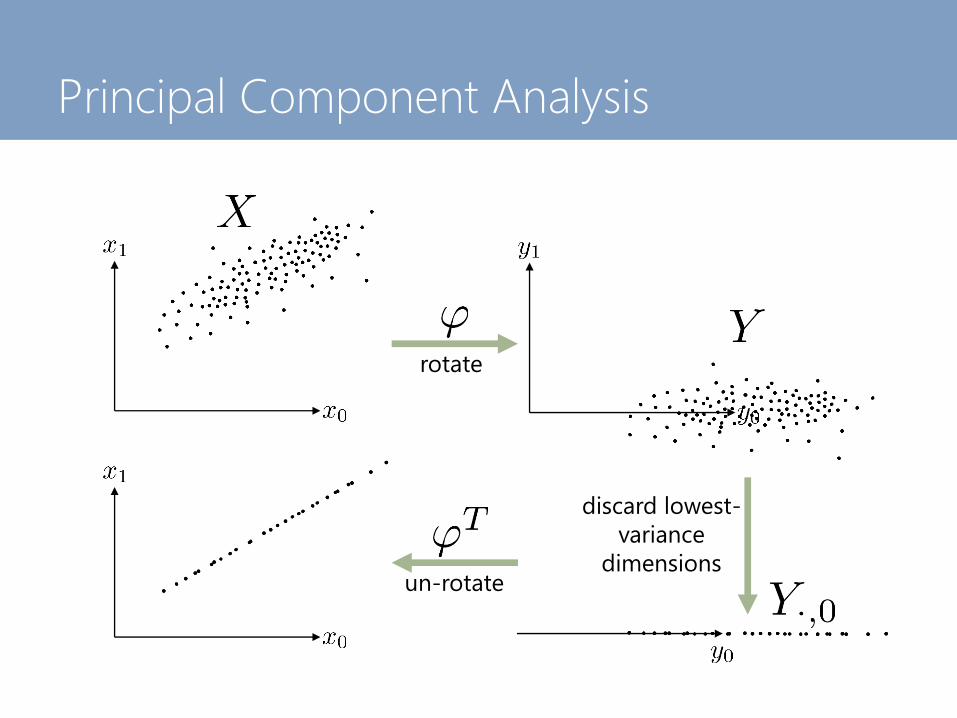
Principal Component Analysis
rotate
discard lowest-
variance
dimensionsun-rotate

Clustering
Q: What would PCA do with this data?
A: Not much, variance is about equal
in all dimensions

K-means Clustering
cluster 3 cluster 4
cluster 1
cluster 2
1. Input is
still a matrix
of features:
2. Output is a
list of cluster
“centroids”:
3. From this we can
describe each point in X
by its cluster membership:
f = [0,0,1,0]f = [0,0,0,1]

Hierarchical clustering
Q: What if our clusters are hierarchical?
Level 1
Level 2

Hierarchical clustering
[0,1,0,0,0,0,0,0,0,0,0,0,0,0,1]
[0,1,0,0,0,0,0,0,0,0,0,0,0,0,1]
[0,1,0,0,0,0,0,0,0,0,0,0,0,1,0]
[0,0,1,0,0,0,0,0,0,0,0,1,0,0,0]
[0,0,1,0,0,0,0,0,0,0,0,1,0,0,0]
[0,0,1,0,0,0,0,0,0,0,1,0,0,0,0]
A: We’d like a representation that encodes that points
have some features in common but not others
Q: What if our clusters are hierarchical?

Hierarchical clustering
Hierarchical (agglomerative) clustering
works by gradually fusing clusters whose
points are closest together
Assign every point to its own cluster:
Clusters = [[1],[2],[3],[4],[5],[6],…,[N]]
While len(Clusters) > 1:
Compute the center of each cluster
Combine the two clusters with the nearest centers

Hierarchical clustering (e.g.)

Hierarchical clustering
If we keep track of the order in which
clusters were merged, we can build a
“hierarchy” of clusters
1 2 43 6 875
43 6 7
6 75
6 75 8
432
4321
6 75 84321
(“dendrogram”)

Hierarchical clustering
Splitting the dendrogram at different
points defines cluster “levels” from which
we can build our feature representation
1 2 43 6 875
43 6 7
6 75
6 75 8
432
4321
6 75 84321
Level 1
Level 2
Level 3
1: [0,0,0,0,1,0]
2: [0,0,1,0,1,0]
3: [1,0,1,0,1,0]
4: [1,0,1,0,1,0]
5: [0,0,0,1,0,1]
6: [0,1,0,1,0,1]
7: [0,1,0,1,0,1]
8: [0,0,0,0,0,1]
L1, L2, L3

Model selection
• Q: How to choose K in K-means?(or:
• How to choose how many PCA dimensions to keep?
• How to choose at what position to “cut” our
hierarchical clusters?
• (later) how to choose how many communities to
look for in a network)

Model selection
1) As a means of “compressing” our data• Choose however many dimensions we can afford to
obtain a given file size/compression ratio
• Keep adding dimensions until adding more no longer
decreases the reconstruction error significantly
# of dimensions
MSE

Model selection
2) As a means of generating potentially
useful features for some other predictive
task (which is what we’re more interested
in in a predictive analytics course!)• Increasing the number of dimensions/number of
clusters gives us additional features to work with, i.e., a
longer feature vector
• In some settings, we may be running an algorithm
whose complexity (either time or memory) scales with
the feature dimensionality (such as we saw last week!);
in this case we would just take however many
dimensions we can afford

Model selection
• Otherwise, we should choose however many
dimensions results in the best prediction performance
on held out data
# of dimensions
MSE (
on
tra
inin
g s
et)
# of dimensionsMSE (
on
vali
dati
on
set)

Questions?
Further reading:• Ricardo Gutierrez-Osuna’s PCA slides (slightly more
mathsy than mine):http://research.cs.tamu.edu/prism/lectures/pr/pr_l9.pdf
• Relationship between PCA and K-means:http://ranger.uta.edu/~chqding/papers/KmeansPCA1.pdf
http://ranger.uta.edu/~chqding/papers/Zha-Kmeans.pdf

Community detection versus clustering
So far we have seen methods
to reduce the dimension of
points based on their features
Principal Component Analysis
rotate
discard lowest-
variance
dimensionsun-rotate

K-means Clustering
cluster 3 cluster 4
cluster 1
cluster 2
1. Input is
still a matrix
of features:
2. Output is a
list of cluster
“centroids”:
3. From this we can
describe each point in X
by its cluster membership:
f = [0,0,1,0]f = [0,0,0,1]

Community detection versus clustering
So far we have seen methods
to reduce the dimension of
points based on their features
What if points are not defined
by features but by their
relationships to each other?

Community detection versus clustering
Q: how can we compactly represent
the set of relationships in a graph?

Community detection versus clustering
A: by representing the nodes in terms
of the communities they belong to

Community detection
(from previous lecture)
communities
f = [0,0,0,1] (A,B,C,D)
e.g. from a PPI network; Yang, McAuley, & Leskovec (2014)
f = [0,0,1,1] (A,B,C,D)

Community detection versus clustering
Part 1 – Clustering
Group sets of points based on
their features
Part 2 – Community detection
Group sets of points based on
their connectivity
Warning: These are rough distinctions that don’t cover all cases. E.g. if
I treat a row of an adjacency matrix as a “feature” and run hierarchical
clustering on it, am I doing clustering or community detection?

Community detection
How should a “community” be defined?

Community detection
How should a “community” be defined?
1. Members should be connected
2. Few edges between communities
3. “Cliqueishness”
4. Dense inside, few edges outside

Today
1. Connected components(members should be connected)
2. Minimum cut(few edges between communities)
3. Clique percolation(“cliqueishness”)
4. Network modularity(dense inside, few edges outside)
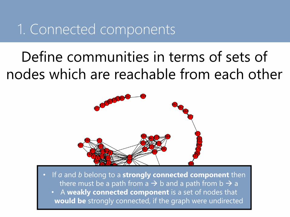
1. Connected components
Define communities in terms of sets of
nodes which are reachable from each other
• If a and b belong to a strongly connected component then
there must be a path from a b and a path from b a
• A weakly connected component is a set of nodes that
would be strongly connected, if the graph were undirected

1. Connected components
• Captures about the roughest notion of
“community” that we could imagine
• Not useful for (most) real graphs:
there will usually be a “giant
component” containing almost all
nodes, which is not really a
community in any reasonable sense

2. Graph cuts
e.g. “Zachary’s Karate Club” (1970)
Picture from http://spaghetti-os.blogspot.com/2014/05/zacharys-karate-club.html
What if the separation between
communities isn’t so clear?
instructor
club president

2. Graph cuts
http://networkkarate.tumblr.com/
Aside: Zachary’s Karate Club Club

2. Graph cuts
Cut the network into two partitions
such that the number of edges
crossed by the cut is minimal
Solution will be degenerate – we need additional constraints
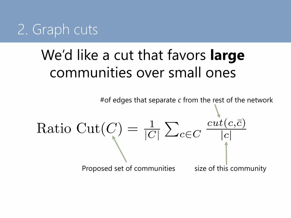
2. Graph cuts
We’d like a cut that favors large
communities over small ones
Proposed set of communities
#of edges that separate c from the rest of the network
size of this community

2. Graph cuts
What is the Ratio Cut cost of the
following two cuts?

2. Graph cuts
But what about…

2. Graph cuts
Maybe rather than counting all
nodes equally in a community, we
should give additional weight to
“influential”, or high-degree nodes
nodes of high degree will have more influence in the denominator

2. Graph cuts
What is the Normalized Cut cost of
the following two cuts?
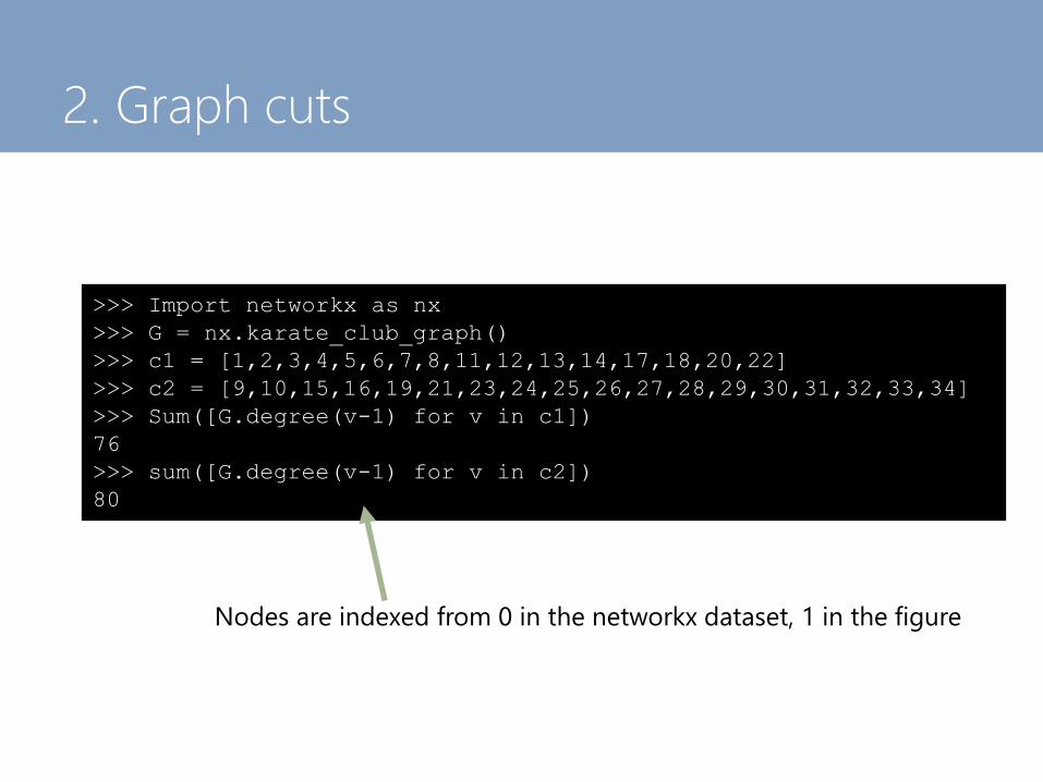
2. Graph cuts
>>> Import networkx as nx
>>> G = nx.karate_club_graph()
>>> c1 = [1,2,3,4,5,6,7,8,11,12,13,14,17,18,20,22]
>>> c2 = [9,10,15,16,19,21,23,24,25,26,27,28,29,30,31,32,33,34]
>>> Sum([G.degree(v-1) for v in c1])
76
>>> sum([G.degree(v-1) for v in c2])
80
Nodes are indexed from 0 in the networkx dataset, 1 in the figure

2. Graph cuts
So what actually happened?
• = Optimal cut
• Red/blue = actual split

Normalized cuts in Computer Vision
“Normalized Cuts and Image Segmentation”
Shi and Malik, 1998

Disjoint communities
Graph data from Adamic (2004). Visualization from allthingsgraphed.com
Separating networks into disjoint
subsets seems to make sense when
communities are somehow “adversarial”
E.g. links between democratic/republican political blogs
(from Adamic, 2004)

Social communities
But what about communities in
social networks (for example)?
e.g. the graph of my facebook friends:
http://jmcauley.ucsd.edu/cse158/data/facebook/egonet.txt

Social communities
Such graphs might have:
• Disjoint communities (i.e., groups of friends who don’t know each other)
e.g. my American friends and my Australian friends
• Overlapping communities (i.e., groups with some intersection)
e.g. my friends and my girlfriend’s friends
• Nested communities (i.e., one group within another)
e.g. my UCSD friends and my CSE friends

3. Clique percolation
How can we define an algorithm that
handles all three types of community
(disjoint/overlapping/nested)?
Clique percolation is one such
algorithm, that discovers communities
based on their “cliqueishness”

3. Clique percolation
1. Given a clique size K
2. Initialize every K-clique as its own community
3. While (two communities I and J have a (K-1)-clique in common):
4. Merge I and J into a single community
• Clique percolation searches for “cliques” in the
network of a certain size (K). Initially each of these
cliques is considered to be its own community
• If two communities share a (K-1) clique in
common, they are merged into a single community
• This process repeats until no more communities
can be merged

3. Clique percolation

What is a “good” community algorithm?
• So far we’ve just defined algorithms to match
some (hopefully reasonable) intuition of what
communities should “look like”
• But how do we know if one definition is better
than another? I.e., how do we evaluate a
community detection algorithm?
• Can we define a probabilistic model
and evaluate the likelihood of
observing a certain set of communities
compared to some null model

4. Network modularity
Null model:
Edges are equally likely between
any pair of nodes, regardless of
community structure
(“Erdos-Renyi random model”)

4. Network modularity
Null model:
Edges are equally likely between
any pair of nodes, regardless of
community structure
(“Erdos-Renyi random model”)
Q: How much does a proposed
set of communities deviate from
this null model?

4. Network modularity

4. Network modularity
Fraction of
edges in
community k
Fraction that we would
expect if edges were
allocated randomly

4. Network modularity

4. Network modularity

4. Network modularity

4. Network modularity
Far fewer edges in
communities than we would
expect at random
Far more edges in
communities than we would
expect at random

4. Network modularity
Algorithm: Choose communities so that the
deviation from the null model is maximized
That is, choose communities such that
maximally many edges are within communities
and minimally many edges cross them
(NP Hard, have to approximate)

Summary
• Community detection aims to summarize the
structure in networks(as opposed to clustering which aims to summarize feature
dimensions)
• Communities can be defined in various ways,
depending on the type of network in question1. Members should be connected (connected components)
2. Few edges between communities (minimum cut)
3. “Cliqueishness” (clique percolation)
4. Dense inside, few edges outside (network modularity)

Assignment 1
Will be discussed next lecture when we
introduce Recommender Systems

Questions?
Further reading:Just on modularity: http://www.cs.cmu.edu/~ckingsf/bioinfo-
lectures/modularity.pdf
Various community detection algorithms, includes spectral formulation
of ratio and normalized cuts:
http://dmml.asu.edu/cdm/slides/chapter3.pptx