CSCI 1951-G – Optimization Methods in FinancePart 06:

Algorithms for Unconstrained ConvexOptimization

March 9, 2018

1 / 28

This material is covered in S. Boyd, L. Vandenberge’s book ConvexOptimization https://web.stanford.edu/~boyd/cvxbook/.

Some of the materials and the figures are taken from it.

2 / 28

Outline

1 Unconstrained minimization: descent methods

2 Equality constrained minimization: Newton’s method

3 General minimization: Interior point methods

3 / 28

Unconstrained minimization

Consider the unconstrained minimization problem:

min f(x)

where f : Rn → R, convex and twice continuously di�erentiable.

x∗: optimal solution with optimal obj. value p∗.

Necessary and su�icient condition for x∗ to be optimal:

∇f(x∗) = 0

The above is a system of . . .n equations in . . .n variables.

Solving ∇f(x) = 0 analytically is o�en not easy or not possible.

4 / 28

Example: unconstrained geometric program

min f(x) = ln

(m∑

i=1

exp(aTi x+ bi)

)

f(x) is convex.

The optimality condition is

0 = ∇f(x∗) =1∑m

j=1 exp(aTj x∗ + bj)

m∑

i=1

exp(aTi x∗ + bi)ai

which in general has no analytical solution.

5 / 28

Iterative algorithms

Iterative algorithms for minimization compute a minimizingsequence

x(0), x(1), . . .

of feasible points s.t.

f(x(k) → p∗ as k →∞

The algorithm terminates when

f(x(k))− p∗ ≤ ε,

for a specified tolerance ε > 0.

6 / 28

How to know when to stop?

Consider the sublevel set

S = {x : f(x) ≤ f(x(0))}

Additional assumption: f is strongly convex on S, i.e., there existm > 0 s.t.

∇2f(x)−mI > 0 for all x ∈ Si.e., the di�erence on the l.h.s. is positive definite.

Consequence:

f(y) ≥ f(x) +∇f(x)T(y − x) +m

2‖y − x‖22 for all x and y in S.

(What happens when f is “just” convex?)

7 / 28

Strong convexity gives a stopping rule

f(y) ≥ f(x) +∇f(x)T(y − x) +m

2‖y − x‖22

For any fixed x, the r.h.s. is a convex quadratic function gx(y) of y.

Let’s find the y for which the r.h.s. is minimal. How?Solve∇gx(y) = 0! Solution:

y = x− 1

m∇f(x)

Then:

f(y) ≥ f(x) +∇f(x)T(y − x) +m

2‖y − x‖22

= f(x)− 1

2m‖∇f(x)‖22

8 / 28

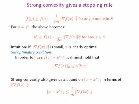
Strong convexity gives a stopping rule

f(y) ≥ f(x)− 1

2m‖∇f(x)‖22 for any x and y in S

For y = x∗, the above becomes:

p∗ ≥ f(x)− 1

2m‖∇f(x)‖22 for any x ∈ S

Intuition: if ‖∇f(x)‖22 is small, x is nearly optimal.Suboptimality condition:

In order to have f(x)− p∗ ≤ ε, it must hold that

‖∇f(x)‖2 ≤√

2mε

Strong convexity also gives us a bound on ‖x− x∗‖2 in terms of‖∇f(x)‖2:

‖x− x∗‖2 ≤2

m‖∇f(x)‖2

9 / 28

Descent methods

We now describe algorithms producing a minimizing sequence(x

(k)k≥1 where

x(k+1) = x(k) + t(k)∆x(k)

• ∆x(k) ∈ Rn (vector): step/search direction.

• t(k) > 0 (scalar): step size/length.

The algorithms are descent methods, i.e.,

f(x(k+1)) < f(x(k))

10 / 28

Descent direction

How to chose ∆x(k) so that f(x(k+1)) < f(x(k))? From convexitywe know that

∇f(x(k))T(y − x(k)) ≥ 0⇒ f(y) . . . ≥ f(x(k))

so ∆x(k) must satisfy:

∇f(x(k))T∆x(k) < 0

I.e., the angle between −∇f(x(k)) and ∆x(k) must be . . . acute.

Such a direction is known as a descent direction.

11 / 28

General descent method

input: function f , starting point xrepeat1 Determine a descent direction ∆x;

2 Line search: choose a step size t ≥ 0;

3 Update: x← x+ t∆x;until stopping criterion is satisfied

Step 2 is called line search because it determines where on the ray

{x+ t∆x : t ≥ 0}

the next iterate will be.

12 / 28

Exact line search

Choose t to minimize f along the ray {x+ t∆x : t ≥ 0}:

t = arg mins≥0

f(x+ s∆x)

Useful when the cost of the above minimization problem is loww.r.t. computing ∆x (e.g., analytical solution)

13 / 28

Backtracking line search

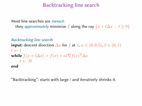
Most line searches are inexact:they approximately minimize f along the ray {x+ t∆x : t ≥ 0}

Backtracking line search:input: descent direction ∆x for f at x, α ∈ (0, 0.5), β ∈ (0, 1)t← 1while f(x+ t∆x) > f(x) + αt∇f(x)T∆x

t← βtend

“Backtracking”: starts with large t and iteratively shrinks it.

14 / 28

Why does backtracking line search terminate?

For small t,f(x+ t∆x) ≈ f(x) + t∇f(x)T∆x

It holds

f(x) + t∇f(x)T∆x < f(x) + αt∇f(x)T∆x

because∇f(x)T∆x ≤ 0

because ∆x is a descent direction.

15 / 28

Visualization9.2 Descent methods 465

t

f(x + t∆x)

t = 0 t0

f(x) + αt∇f(x)T∆xf(x) + t∇f(x)T∆x

Figure 9.1 Backtracking line search. The curve shows f , restricted to the lineover which we search. The lower dashed line shows the linear extrapolationof f , and the upper dashed line has a slope a factor of α smaller. Thebacktracking condition is that f lies below the upper dashed line, i.e., 0 ≤t ≤ t0.

The line search is called backtracking because it starts with unit step size andthen reduces it by the factor β until the stopping condition f(x + t∆x) ≤ f(x) +αt∇f(x)T∆x holds. Since ∆x is a descent direction, we have ∇f(x)T∆x < 0, sofor small enough t we have

f(x + t∆x) ≈ f(x) + t∇f(x)T∆x < f(x) + αt∇f(x)T∆x,

which shows that the backtracking line search eventually terminates. The constantα can be interpreted as the fraction of the decrease in f predicted by linear extrap-olation that we will accept. (The reason for requiring α to be smaller than 0.5 willbecome clear later.)

The backtracking condition is illustrated in figure 9.1. This figure suggests,and it can be shown, that the backtracking exit inequality f(x + t∆x) ≤ f(x) +αt∇f(x)T∆x holds for t ≥ 0 in an interval (0, t0]. It follows that the backtrackingline search stops with a step length t that satisfies

t = 1, or t ∈ (βt0, t0].

The first case occurs when the step length t = 1 satisfies the backtracking condition,i.e., 1 ≤ t0. In particular, we can say that the step length obtained by backtrackingline search satisfies

t ≥ min{1,βt0}.

When dom f is not all of Rn, the condition f(x+ t∆x) ≤ f(x)+αt∇f(x)T∆xin the backtracking line search must be interpreted carefully. By our conventionthat f is infinite outside its domain, the inequality implies that x + t∆x ∈ dom f .In a practical implementation, we first multiply t by β until x + t∆x ∈ dom f ;

16 / 28

Gradient descent method

input: function f , starting point xrepeat1 ∆x← −∇f(x);

2 Line search: choose a step size t ≥ 0 via exact or backtracking linesearch;

3 Update: x← x+ t∆x;until stopping criterion is satisfied (e.g., ‖∇f(x)‖2 ≤ η)

17 / 28

Example

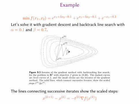
min f(x1, x2) = ex1+3x2−0.1 + ex1−3x2−0.1 + e−x1−0.1

Let’s solve it with gradient descent and backtrack line search withα = 0.1 and β = 0.7.

9.3 Gradient descent method 471

x(0)

x(1)

x(2)

Figure 9.3 Iterates of the gradient method with backtracking line search,for the problem in R2 with objective f given in (9.20). The dashed curvesare level curves of f , and the small circles are the iterates of the gradientmethod. The solid lines, which connect successive iterates, show the scaledsteps t(k)∆x(k).

k

f(x

(k))−

p⋆

backtracking l.s.

exact l.s.

0 5 10 15 20 2510−15

10−10

10−5

100

105

Figure 9.4 Error f(x(k))− p⋆ versus iteration k of the gradient method withbacktracking and exact line search, for the problem in R2 with objective fgiven in (9.20). The plot shows nearly linear convergence, with the errorreduced approximately by the factor 0.4 in each iteration of the gradientmethod with backtracking line search, and by the factor 0.2 in each iterationof the gradient method with exact line search.

The lines connecting successive iterates show the scaled steps:

x(k+1) − x(k) = −t(k)∇f(x(k))18 / 28

Example

472 9 Unconstrained minimization

x(0)

x(1)

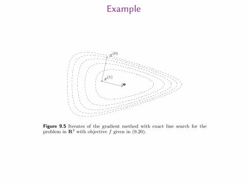
Figure 9.5 Iterates of the gradient method with exact line search for theproblem in R2 with objective f given in (9.20).

A problem in R100

We next consider a larger example, of the form

f(x) = cT x−m∑

i=1

log(bi − aTi x), (9.21)

with m = 500 terms and n = 100 variables.

The progress of the gradient method with backtracking line search, with pa-rameters α = 0.1, β = 0.5, is shown in figure 9.6. In this example we see an initialapproximately linear and fairly rapid convergence for about 20 iterations, followedby a slower linear convergence. Overall, the error is reduced by a factor of around106 in around 175 iterations, which gives an average error reduction by a factor ofaround 10−6/175 ≈ 0.92 per iteration. The initial convergence rate, for the first 20iterations, is around a factor of 0.8 per iteration; the slower final convergence rate,after the first 20 iterations, is around a factor of 0.94 per iteration.

Figure 9.6 shows the convergence of the gradient method with exact line search.The convergence is again approximately linear, with an overall error reduction byapproximately a factor 10−6/140 ≈ 0.91 per iteration. This is only a bit faster thanthe gradient method with backtracking line search.

Finally, we examine the influence of the backtracking line search parameters αand β on the convergence rate, by determining the number of iterations requiredto obtain f(x(k)) − p⋆ ≤ 10−5. In the first experiment, we fix β = 0.5, and varyα from 0.05 to 0.5. The number of iterations required varies from about 80, forlarger values of α, in the range 0.2–0.5, to about 170 for smaller values of α. This,and other experiments, suggest that the gradient method works better with fairlylarge α, in the range 0.2–0.5.

Similarly, we can study the effect of the choice of β by fixing α = 0.1 andvarying β from 0.05 to 0.95. Again the variation in the total number of iterationsis not large, ranging from around 80 (when β ≈ 0.5) to around 200 (for β small,or near 1). This experiment, and others, suggest that β ≈ 0.5 is a good choice.

19 / 28

Example

9.3 Gradient descent method 471

x(0)

x(1)

x(2)

Figure 9.3 Iterates of the gradient method with backtracking line search,for the problem in R2 with objective f given in (9.20). The dashed curvesare level curves of f , and the small circles are the iterates of the gradientmethod. The solid lines, which connect successive iterates, show the scaledsteps t(k)∆x(k).

k

f(x

(k))−

p⋆

backtracking l.s.

exact l.s.

0 5 10 15 20 2510−15

10−10

10−5

100

105

Figure 9.4 Error f(x(k))− p⋆ versus iteration k of the gradient method withbacktracking and exact line search, for the problem in R2 with objective fgiven in (9.20). The plot shows nearly linear convergence, with the errorreduced approximately by the factor 0.4 in each iteration of the gradientmethod with backtracking line search, and by the factor 0.2 in each iterationof the gradient method with exact line search.

20 / 28

Convergence analysisFact: if f is strongly convex on S, then

∃M ∈ R+ s.t. ∇2f(x) ≤MI , for all x ∈ S.Converge of gradient descent:Let ε > 0. Let

k ≥ log

(f(x(0))− p∗

ε

)1

− log(1− m

M

)

A�er k iterations it must hold

f(x(k))− p∗ ≤ ε

More interpretable bound:

f(x(k))− p∗ ≤(

1− m

M

)(f(x(0))− p∗)

I.e., the error converges to 0 at least as fast as a geometric series(linear convergence (on a log-linear plot))

21 / 28

Steepest descent method

We saw that gradient descent may converge very slowly if M/m islarge.

Is the gradient the best descent direction to take (and in whatsense)?First-order Taylor approximation of f(x+ v) around x:

f(x+ v) ≈ f(x) +∇f(x)Tv

∇f(x)Tv is the directional derivative of f at x in the direction v

22 / 28

Steepest descent method

v is a descent direction if the directional derivative∇f(x)Tv isnegative.

How to choose v to make the directional derivative as negative aspossible?

Since ∇f(x)Tv is linear in v, we must restrict the choice of vsomehow (oth. . . .we could just keep growing the magnitude of v)

Let ‖ · ‖ be any norm in Rn

Normalized steepest descent direction w.r.t. ‖ · ‖:

∆xnsd = arg min{∇f(x)Tv : ‖v‖ = 1}

It gives the largest decrease in the linear approximation of f

23 / 28

Example

If ‖ · ‖ is the Euclidean norm, then

∆xnsd = −∇f(x)

24 / 28

Example

Consider the quadratic norm

‖z‖P = (zTPz)1/2 = ‖P 1/2z‖2

where P is positive definite.

The normalized steepest descent direction is

∆xnsd = (∇f(x)TP−1∇f(x))1/2P−1∇f(x)

for the step v = −P−1∇f(x).

25 / 28

Geometric interpretation

9.4 Steepest descent method 477

−∇f(x)

∆xnsd

Figure 9.9 Normalized steepest descent direction for a quadratic norm. Theellipsoid shown is the unit ball of the norm, translated to the point x. Thenormalized steepest descent direction ∆xnsd at x extends as far as possiblein the direction −∇f(x) while staying in the ellipsoid. The gradient andnormalized steepest descent directions are shown.

Interpretation via change of coordinates

We can give an interesting alternative interpretation of the steepest descent direc-tion ∆xsd as the gradient search direction after a change of coordinates is appliedto the problem. Define u = P 1/2u, so we have ∥u∥P = ∥u∥2. Using this changeof coordinates, we can solve the original problem of minimizing f by solving theequivalent problem of minimizing the function f : Rn → R, given by

f(u) = f(P−1/2u) = f(u).

If we apply the gradient method to f , the search direction at a point x (whichcorresponds to the point x = P−1/2x for the original problem) is

∆x = −∇f(x) = −P−1/2∇f(P−1/2x) = −P−1/2∇f(x).

This gradient search direction corresponds to the direction

∆x = P−1/2(−P−1/2∇f(x)

)= −P−1∇f(x)

for the original variable x. In other words, the steepest descent method in thequadratic norm ∥ · ∥P can be thought of as the gradient method applied to theproblem after the change of coordinates x = P 1/2x.

9.4.2 Steepest descent for ℓ1-norm

As another example, we consider the steepest descent method for the ℓ1-norm. Anormalized steepest descent direction,

∆xnsd = argmin{∇f(x)T v | ∥v∥1 ≤ 1},

26 / 28

Coordinate-descent

Let ‖ · ‖ be the `1 norm. Let i be any index for which

‖∇f(x)‖∞ = |(∇f(x))i|

then

∆xnsd = −sign(∂f(x)

∂xi

)ei

where ei is the ith standard basis vector.Thus, only one component of x is going to change!

This can greatly simplify the line search step.

27 / 28

Geometric interpretation

478 9 Unconstrained minimization

−∇f(x)

∆xnsd

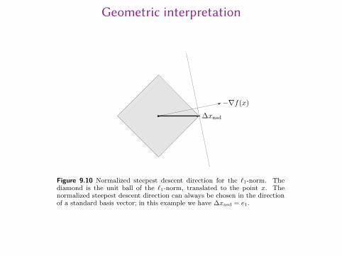
Figure 9.10 Normalized steepest descent direction for the ℓ1-norm. Thediamond is the unit ball of the ℓ1-norm, translated to the point x. Thenormalized steepest descent direction can always be chosen in the directionof a standard basis vector; in this example we have ∆xnsd = e1.

is easily characterized. Let i be any index for which ∥∇f(x)∥∞ = |(∇f(x))i|. Thena normalized steepest descent direction ∆xnsd for the ℓ1-norm is given by

∆xnsd = −sign

(∂f(x)

∂xi

)ei,

where ei is the ith standard basis vector. An unnormalized steepest descent stepis then

∆xsd = ∆xnsd∥∇f(x)∥∞ = −∂f(x)

∂xiei.

Thus, the normalized steepest descent step in ℓ1-norm can always be chosen to be astandard basis vector (or a negative standard basis vector). It is the coordinate axisdirection along which the approximate decrease in f is greatest. This is illustratedin figure 9.10.

The steepest descent algorithm in the ℓ1-norm has a very natural interpretation:At each iteration we select a component of ∇f(x) with maximum absolute value,and then decrease or increase the corresponding component of x, according to thesign of (∇f(x))i. The algorithm is sometimes called a coordinate-descent algorithm,since only one component of the variable x is updated at each iteration. This cangreatly simplify, or even trivialize, the line search.

Example 9.2 Frobenius norm scaling. In §4.5.4 we encountered the unconstrainedgeometric program

minimize∑n

i,j=1M2

ijd2i /d2

j ,

where M ∈ Rn×n is given, and the variable is d ∈ Rn. Using the change of variablesxi = 2 log di we can express this geometric program in convex form as

minimize f(x) = log(∑n

i,j=1M2

ijexi−xj

).

28 / 28