csc321 lecture 22: q-learning
TRANSCRIPT
CSC321 Lecture 22: Q-Learning
Roger Grosse
Roger Grosse CSC321 Lecture 22: Q-Learning 1 / 21
Overview
Second of 3 lectures on reinforcement learning
Last time: policy gradient (e.g. REINFORCE)
Optimize a policy directly, don’t represent anything about theenvironment
Today: Q-learning
Learn an action-value function that predicts future returns
Next time: AlphaGo uses both a policy network and a value network
This lecture is review if you’ve taken 411
This lecture has more new content than I’d intended. If there is anexam question about this lecture or next one, it won’t be a hardquestion.
Roger Grosse CSC321 Lecture 22: Q-Learning 2 / 21
Overview
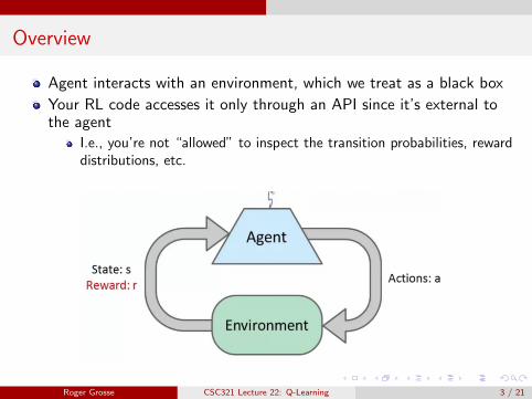
Agent interacts with an environment, which we treat as a black box
Your RL code accesses it only through an API since it’s external tothe agent
I.e., you’re not “allowed” to inspect the transition probabilities, rewarddistributions, etc.
Roger Grosse CSC321 Lecture 22: Q-Learning 3 / 21
Recap: Markov Decision Processes
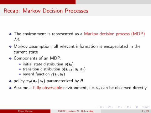
The environment is represented as a Markov decision process (MDP)M.
Markov assumption: all relevant information is encapsulated in thecurrent state
Components of an MDP:
initial state distribution p(s0)transition distribution p(st+1 | st , at)reward function r(st , at)
policy πθ(at | st) parameterized by θ
Assume a fully observable environment, i.e. st can be observed directly
Roger Grosse CSC321 Lecture 22: Q-Learning 4 / 21
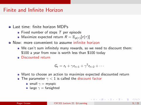
Finite and Infinite Horizon
Last time: finite horizon MDPs
Fixed number of steps T per episodeMaximize expected return R = Ep(τ)[r(τ)]
Now: more convenient to assume infinite horizon
We can’t sum infinitely many rewards, so we need to discount them:$100 a year from now is worth less than $100 todayDiscounted return
Gt = rt + γrt+1 + γ2rt+2 + · · ·
Want to choose an action to maximize expected discounted returnThe parameter γ < 1 is called the discount factor
small γ = myopiclarge γ = farsighted
Roger Grosse CSC321 Lecture 22: Q-Learning 5 / 21
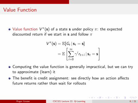
Value Function
Value function V π(s) of a state s under policy π: the expecteddiscounted return if we start in s and follow π
V π(s) = E[Gt | st = s]
= E
[ ∞∑i=0
γ i rt+i | st = s
]
Computing the value function is generally impractical, but we can tryto approximate (learn) it
The benefit is credit assignment: see directly how an action affectsfuture returns rather than wait for rollouts
Roger Grosse CSC321 Lecture 22: Q-Learning 6 / 21
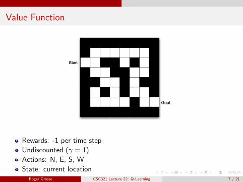
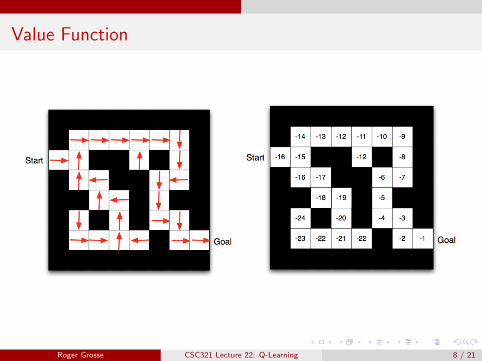
Value Function
Rewards: -1 per time step
Undiscounted (γ = 1)
Actions: N, E, S, W
State: current locationRoger Grosse CSC321 Lecture 22: Q-Learning 7 / 21
Value Function
Roger Grosse CSC321 Lecture 22: Q-Learning 8 / 21
Action-Value Function
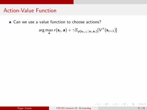
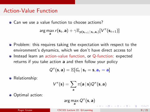
Can we use a value function to choose actions?
arg maxa
r(st , a) + γEp(st+1 | st ,at)[Vπ(st+1)]
Problem: this requires taking the expectation with respect to theenvironment’s dynamics, which we don’t have direct access to!
Instead learn an action-value function, or Q-function: expectedreturns if you take action a and then follow your policy
Qπ(s, a) = E[Gt | st = s, at = a]
Relationship:
V π(s) =∑a
π(a | s)Qπ(s, a)
Optimal action:arg max
aQπ(s, a)
Roger Grosse CSC321 Lecture 22: Q-Learning 9 / 21
Action-Value Function
Can we use a value function to choose actions?
arg maxa
r(st , a) + γEp(st+1 | st ,at)[Vπ(st+1)]
Problem: this requires taking the expectation with respect to theenvironment’s dynamics, which we don’t have direct access to!
Instead learn an action-value function, or Q-function: expectedreturns if you take action a and then follow your policy
Qπ(s, a) = E[Gt | st = s, at = a]
Relationship:
V π(s) =∑a
π(a | s)Qπ(s, a)
Optimal action:arg max
aQπ(s, a)
Roger Grosse CSC321 Lecture 22: Q-Learning 9 / 21
Bellman Equation
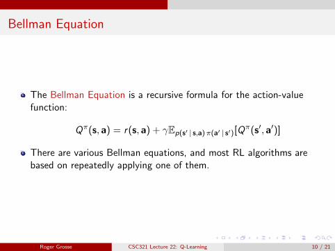
The Bellman Equation is a recursive formula for the action-valuefunction:
Qπ(s, a) = r(s, a) + γEp(s′ | s,a)π(a′ | s′)[Qπ(s′, a′)]
There are various Bellman equations, and most RL algorithms arebased on repeatedly applying one of them.
Roger Grosse CSC321 Lecture 22: Q-Learning 10 / 21
Optimal Bellman Equation
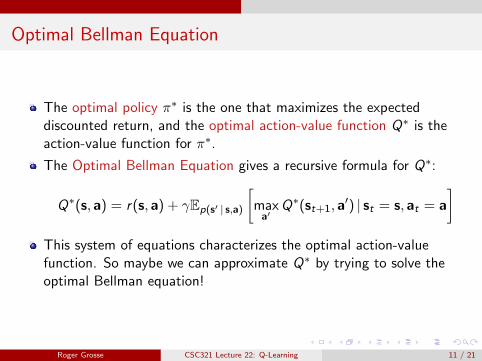
The optimal policy π∗ is the one that maximizes the expecteddiscounted return, and the optimal action-value function Q∗ is theaction-value function for π∗.
The Optimal Bellman Equation gives a recursive formula for Q∗:
Q∗(s, a) = r(s, a) + γEp(s′ | s,a)
[maxa′
Q∗(st+1, a′) | st = s, at = a
]This system of equations characterizes the optimal action-valuefunction. So maybe we can approximate Q∗ by trying to solve theoptimal Bellman equation!
Roger Grosse CSC321 Lecture 22: Q-Learning 11 / 21
Q-Learning
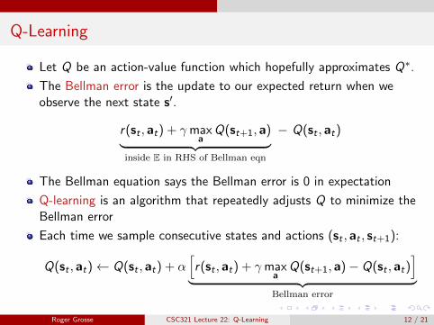
Let Q be an action-value function which hopefully approximates Q∗.
The Bellman error is the update to our expected return when weobserve the next state s′.
r(st , at) + γmaxa
Q(st+1, a)︸ ︷︷ ︸inside E in RHS of Bellman eqn
− Q(st , at)
The Bellman equation says the Bellman error is 0 in expectation
Q-learning is an algorithm that repeatedly adjusts Q to minimize theBellman error
Each time we sample consecutive states and actions (st , at , st+1):
Q(st , at)← Q(st , at) + α[r(st , at) + γmax
aQ(st+1, a)− Q(st , at)
]︸ ︷︷ ︸
Bellman error
Roger Grosse CSC321 Lecture 22: Q-Learning 12 / 21
Exploration-Exploitation Tradeoff
Notice: Q-learning only learns about the states and actions it visits.
Exploration-exploitation tradeoff: the agent should sometimes picksuboptimal actions in order to visit new states and actions.
Simple solution: ε-greedy policy
With probability 1− ε, choose the optimal action according to QWith probability ε, choose a random action
Believe it or not, ε-greedy is still used today!
Roger Grosse CSC321 Lecture 22: Q-Learning 13 / 21
Exploration-Exploitation Tradeoff
You can’t use an epsilon-greedy strategy with policy gradient becauseit’s an on-policy algorithm: the agent can only learn about the policyit’s actually following.
Q-learning is an off-policy algorithm: the agent can learn Q regardlessof whether it’s actually following the optimal policy
Hence, Q-learning is typically done with an ε-greedy policy, or someother policy that encourages exploration.
Roger Grosse CSC321 Lecture 22: Q-Learning 14 / 21
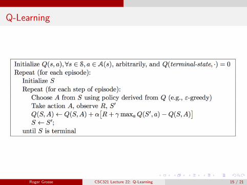
Q-Learning
Roger Grosse CSC321 Lecture 22: Q-Learning 15 / 21
Function Approximation
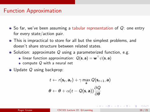
So far, we’ve been assuming a tabular representation of Q: one entryfor every state/action pair.
This is impractical to store for all but the simplest problems, anddoesn’t share structure between related states.
Solution: approximate Q using a parameterized function, e.g.
linear function approximation: Q(s, a) = w>ψ(s, a)compute Q with a neural net
Update Q using backprop:
t ← r(st , at) + γmaxa
Q(st+1, a)
θ ← θ + α(t − Q(s, a))∂Q
∂θ
Roger Grosse CSC321 Lecture 22: Q-Learning 16 / 21
Function Approximation
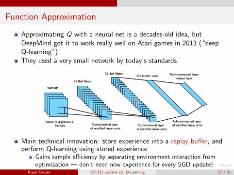
Approximating Q with a neural net is a decades-old idea, butDeepMind got it to work really well on Atari games in 2013 (“deepQ-learning”)They used a very small network by today’s standards
Main technical innovation: store experience into a replay buffer, andperform Q-learning using stored experience
Gains sample efficiency by separating environment interaction fromoptimization — don’t need new experience for every SGD update!
Roger Grosse CSC321 Lecture 22: Q-Learning 17 / 21
Atari
Mnih et al., Nature 2015. Human-level control through deepreinforcement learning
Network was given raw pixels as observations
Same architecture shared between all games
Assume fully observable environment, even though that’s not the case
After about a day of training on a particular game, often beat“human-level” performance (number of points within 5 minutes ofplay)
Did very well on reactive games, poorly on ones that require planning(e.g. Montezuma’s Revenge)
https://www.youtube.com/watch?v=V1eYniJ0Rnk
https://www.youtube.com/watch?v=4MlZncshy1Q
Roger Grosse CSC321 Lecture 22: Q-Learning 18 / 21
Wireheading
If rats have a lever that causes an electrode to stimulate certain“reward centers” in their brain, they’ll keep pressing the lever at theexpense of sleep, food, etc.
RL algorithms show this “wireheading” behavior if the rewardfunction isn’t designed carefully
https://blog.openai.com/faulty-reward-functions/
Roger Grosse CSC321 Lecture 22: Q-Learning 19 / 21
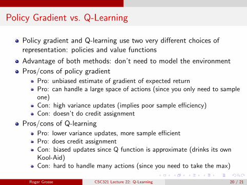
Policy Gradient vs. Q-Learning
Policy gradient and Q-learning use two very different choices ofrepresentation: policies and value functions
Advantage of both methods: don’t need to model the environment
Pros/cons of policy gradient
Pro: unbiased estimate of gradient of expected returnPro: can handle a large space of actions (since you only need to sampleone)Con: high variance updates (implies poor sample efficiency)Con: doesn’t do credit assignment
Pros/cons of Q-learning
Pro: lower variance updates, more sample efficientPro: does credit assignmentCon: biased updates since Q function is approximate (drinks its ownKool-Aid)Con: hard to handle many actions (since you need to take the max)
Roger Grosse CSC321 Lecture 22: Q-Learning 20 / 21
Actor-Critic (optional)
Actor-critic methods combine the best of both worlds
Fit both a policy network (the “actor”) and a value network (the“critic”)
Repeatedly update the value network to estimate V π
Unroll for only a few steps, then compute the REINFORCE policyupdate using the expected returns estimated by the value network
The two networks adapt to each other, much like GAN training
Modern version: Asynchronous Advantage Actor-Critic (A3C)
Roger Grosse CSC321 Lecture 22: Q-Learning 21 / 21