cs7015 (deep learning) : lecture 9miteshk/cs7015/slides/handout/lecture… · mitesh m. khapra...

1/1

CS7015 (Deep Learning) : Lecture 9Greedy Layerwise Pre-training, Better activation functions, Better weight

initialization methods, Batch Normalization

Mitesh M. Khapra

Department of Computer Science and EngineeringIndian Institute of Technology Madras

Mitesh M. Khapra CS7015 (Deep Learning) : Lecture 9

2/1

Module 9.1 : A quick recap of training deep neuralnetworks


3/1

x

σ

w

y

x1x2 x3

σ

y

w1 w2 w3

We already saw how to train this network

w = w − η∇w where,

∇w =∂L (w)

∂w= (f(x)− y) ∗ f(x) ∗ (1− f(x)) ∗ x

What about a wider network with more inputs:

w1 = w1 − η∇w1

w2 = w2 − η∇w2

w3 = w3 − η∇w3

where,∇wi = (f(x)− y) ∗ f(x) ∗ (1− f(x)) ∗ xi


4/1

σ

x = h0

σ

σ

y

w1

w2

w3

a1

h1

a2

h2

a3

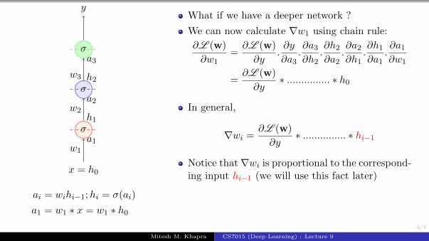
ai = wihi−1;hi = σ(ai)

a1 = w1 ∗ x = w1 ∗ h0

What if we have a deeper network ?

We can now calculate ∇w1 using chain rule:

∂L (w)

∂w1=∂L (w)

∂y.∂y

∂a3.∂a3∂h2

.∂h2∂a2

.∂a2∂h1

.∂h1∂a1

.∂a1∂w1

=∂L (w)

∂y∗ ............... ∗ h0

In general,

∇wi =∂L (w)

∂y∗ ............... ∗ hi−1

Notice that∇wi is proportional to the correspond-ing input hi−1 (we will use this fact later)


5/1

σ

σ

x1

σ σ

x2 x3

σ σ σ

σ

y

w1 w2 w3

What happens if we have a network which is deepand wide?

How do you calculate ∇w2 =?

It will be given by chain rule applied across mul-tiple paths (We saw this in detail when we studiedback propagation)


6/1

Things to remember

Training Neural Networks is a Game of Gradients (played using any of theexisting gradient based approaches that we discussed)

The gradient tells us the responsibility of a parameter towards the loss

The gradient w.r.t. a parameter is proportional to the input to the parameters(recall the “..... ∗ x” term or the “.... ∗ hi” term in the formula for ∇wi)


7/1

σ

σ

x1

σ σ

x2 x3

σ σ σ

σ

y

w1 w2 w3

Backpropagation was made popularby Rumelhart et.al in 1986

However when used for really deepnetworks it was not very successful

In fact, till 2006 it was very hard totrain very deep networks

Typically, even after a large numberof epochs the training did not con-verge


8/1

Module 9.2 : Unsupervised pre-training


9/1

What has changed now? How did Deep Learning become so popular despitethis problem with training large networks?

Well, until 2006 it wasn’t so popular

The field got revived after the seminal work of Hinton and Salakhutdinov in2006

1G. E. Hinton and R. R. Salakhutdinov. Reducing the dimensionality of data with neuralnetworks. Science, 313(5786):504–507, July 2006.


10/1

Let’s look at the idea of unsupervised pre-training introduced in this paper ...(note that in this paper they introduced the idea in the context of RBMs but we

will discuss it in the context of Autoencoders)


11/1

x

h1

x

reconstruct x

min1

m

m∑i=1

n∑j=1

(xij − xij)2

Consider the deep neural networkshown in this figure

Let us focus on the first two layers ofthe network (x and h1)

We will first train the weightsbetween these two layers using an un-supervised objective

Note that we are trying to reconstructthe input (x) from the hidden repres-entation (h1)

We refer to this as an unsupervisedobjective because it does not involvethe output label (y) and only uses theinput data (x)


12/1

h1

h2

h1

x

min1

m

m∑i=1

n∑j=1

(h1ij − h1ij )2

At the end of this step, the weightsin layer 1 are trained such that h1captures an abstract representationof the input x

We now fix the weights in layer 1 andrepeat the same process with layer 2

At the end of this step, the weights inlayer 2 are trained such that h2 cap-tures an abstract representation of h1

We continue this process till the lasthidden layer (i.e., the layer before theoutput layer) so that each successivelayer captures an abstract represent-ation of the previous layer


13/1

x1 x2 x3

minθ

1

m

m∑i=1

(yi − f(xi))2

After this layerwise pre-training, weadd the output layer and train thewhole network using the task specificobjective

Note that, in effect we have initial-ized the weights of the network us-ing the greedy unsupervised objectiveand are now fine tuning these weightsusing the supervised objective


14/1

Why does this work better?

Is it because of better optimization?

Is it because of better regularization?

Let’s see what these two questions mean and try to answer them based on some(among many) existing studies1,2

1The difficulty of training deep architectures and effect of unsupervised pre-training - Erhan etal,2009

2Exploring Strategies for Training Deep Neural Networks, Larocelle et al,2009Mitesh M. Khapra CS7015 (Deep Learning) : Lecture 9

15/1





16/1

What is the optimization problem that we are trying to solve?

minimize L (θ) =1

m

m∑i=1

(yi − f(xi))2

Is it the case that in the absence of unsupervised pre-training we are not ableto drive L (θ) to 0 even for the training data (hence poor optimization) ?

Let us see this in more detail ...


17/1

The error surface of the supervisedobjective of a Deep Neural Networkis highly non-convex

With many hills and plateaus and val-leys

Given that large capacity of DNNs itis still easy to land in one of these 0error regions

Indeed Larochelle et.al.1 show that ifthe last layer has large capacity thenL (θ) goes to 0 even without pre-training

However, if the capacity of the net-work is small, unsupervised pre-training helps

1Exploring Strategies for Training Deep Neural Networks, Larocelle et al,2009Mitesh M. Khapra CS7015 (Deep Learning) : Lecture 9

18/1





19/1

What does regularization do? It con-strains the weights to certain regionsof the parameter space

L-1 regularization: constrains mostweights to be 0

L-2 regularization: prevents mostweights from taking large values

1Image Source:The Elements of Statistical Learning-T. Hastie, R. Tibshirani, and J. Friedman,Pg 71


20/1

Unsupervised objective:

Ω(θ) =1

m

m∑i=1

n∑j=1

(xij − xij)2

We can think of this unsupervised ob-jective as an additional constraint onthe optimization problem

Supervised objective:

L (θ) =1

m

m∑i=1

(yi − f(xi))2

Indeed, pre-training constrains theweights to lie in only certain regionsof the parameter space

Specifically, it constrains the weightsto lie in regions where the character-istics of the data are captured well (asgoverned by the unsupervised object-ive)

This unsupervised objective ensuresthat that the learning is not greedyw.r.t. the supervised objective (andalso satisfies the unsupervised object-ive)


21/1

Some other experiments have alsoshown that pre-training is more ro-bust to random initializations

One accepted hypothesis is that pre-training leads to better weight ini-tializations (so that the layers cap-ture the internal characteristics of thedata)

1The difficulty of training deep architectures and effect of unsupervised pre-training - Erhan etal,2009


22/1

So what has happened since 2006-2009?


23/1

Deep Learning has evolved

Better optimization algorithms

Better regularization methods

Better activation functions

Better weight initialization strategies


24/1

Module 9.3 : Better activation functions


25/1







26/1

Before we look at activation functions, let’s try to answer the following question:“What makes Deep Neural Networks powerful ?”


27/1

h0 = x

y

σ

σ

σ

a1h1

a2h2

a3

w1

w2

w3

Consider this deep neural network

Imagine if we replace the sigmoid ineach layer by a simple linear trans-formation

y = (w4 ∗ (w3 ∗ (w2 ∗ (w1x))))

Then we will just learn y as a lineartransformation of x

In other words we will be constrainedto learning linear decision boundaries

We cannot learn arbitrary decisionboundaries


28/1

In particular, a deep linear neuralnetwork cannot learn such boundar-ies

But a deep non linear neural net-work can indeed learn such bound-aries (recall Universal ApproximationTheorem)


29/1

Now let’s look at some non-linear activation functions that are typically used indeep neural networks (Much of this material is taken from Andrej Karpathy’slecture notes 1)

1http://cs231n.github.ioMitesh M. Khapra CS7015 (Deep Learning) : Lecture 9

30/1

Sigmoid

σ(x) = 11+e−x

As is obvious, the sigmoid functioncompresses all its inputs to the range[0,1]

Since we are always interested ingradients, let us find the gradient ofthis function

∂σ(x)

∂x= σ(x)(1− σ(x))

(you can easily derive it)

Let us see what happens if we use sig-moid in a deep network


31/1

h0 = x

σ

σ

σ

σ

a1h1

a2h2

a3h3

a4h4

a3 = w2h2h3 = σ(a3)

While calculating ∇w2 at some pointin the chain rule we will encounter

∂h3∂a3

=∂σ(a3)

∂a3= σ(a3)(1− σ(a3))

What is the consequence of this ?

To answer this question let us firstunderstand the concept of saturatedneuron ?


32/1

−2 −1 1 2

0.2

0.4

0.6

0.8

1

x

y

Saturated neurons thus cause thegradient to vanish.

A sigmoid neuron is said to have sat-urated when σ(x) = 1 or σ(x) = 0

What would the gradient be at satur-ation?

Well it would be 0 (you can see it fromthe plot or from the formula that wederived)


33/1

Saturated neurons thus cause thegradient to vanish.

w1 w2 w3 w4

σ(∑4

i=1wixi)

−2 −1 1 2

0.2

0.4

0.6

0.8

1

∑4i=1wixi

y

But why would the neurons saturate?

Consider what would happen if weuse sigmoid neurons and initialize theweights to very high values ?

The neurons will saturate veryquickly

The gradients will vanish and thetraining will stall (more on this later)


34/1

Saturated neurons cause the gradientto vanish

Sigmoids are not zero centered

Consider the gradient w.r.t. w1 andw2

∇w1 =∂L (w)

∂y

∂y

h3

∂h3∂a3

∂a3∂w1

h21

∇w2 =∂L (w)

∂y

∂y

h3

∂h3∂a3

∂a3∂w2

h22

Note that h21 and h22 are between[0, 1] (i.e., they are both positive)

So if the first common term (in red)is positive (negative) then both ∇w1

and ∇w2 are positive (negative)

Why is this a problem??

w1 w2

a3 = w1 ∗ h21 + w2 ∗ h22

y

h0 = x

h1

h2

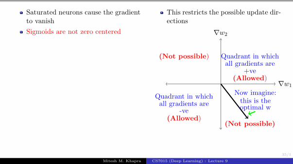
Essentially, either all the gradients ata layer are positive or all the gradientsat a layer are negative


35/1



This restricts the possible update dir-ections

∇w2

∇w1

(Not possible) Quadrant in whichall gradients are

+ve(Allowed)

Quadrant in whichall gradients are

-ve(Allowed)

(Not possible)

Now imagine:this is theoptimal w


36/1



And lastly, sigmoids are compu-tationally expensive (because ofexp (x))

∇w2

∇w1

starting from thisinitial positiononly way to reach it

is by taking a zigzag path


37/1

tanh(x)

0−4 −2 2 4

−1

−0.5

0.5

1

x

y

f(x) = tanh(x)

Compresses all its inputs to the range[-1,1]

Zero centered

What is the derivative of this func-tion?

∂tanh(x)

∂x= (1− tanh2(x))

The gradient still vanishes at satura-tion

Also computationally expensive


38/1

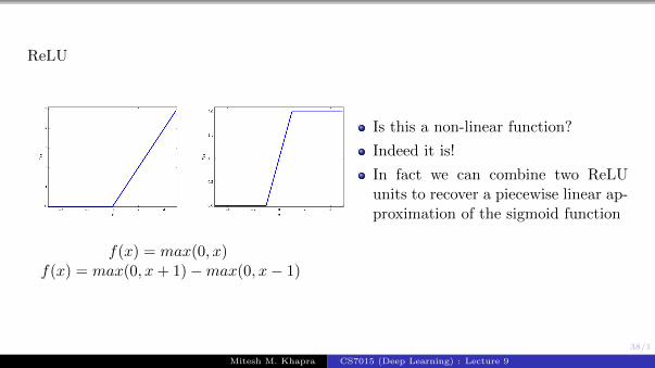
ReLU

f(x) = max(0, x)f(x) = max(0, x+ 1)−max(0, x− 1)

Is this a non-linear function?

Indeed it is!

In fact we can combine two ReLUunits to recover a piecewise linear ap-proximation of the sigmoid function


39/1

ReLU

f(x) = max(0, x)

Advantages of ReLU

Does not saturate in the positive re-gion

Computationally efficient

In practice converges much fasterthan sigmoid/tanh1

1ImageNet Classification with Deep Convolutional Neural Networks- Alex Krizhevsky IlyaSutskever, Geoffrey E. Hinton, 2012


40/1

x1 x2 1

y

w1 w2 b

h1a1

a2w3

In practice there is a caveat

Let’s see what is the derivative of ReLU(x)

∂ReLU(x)

∂x= 0 if x < 0

= 1 if x > 0

Now consider the given network

What would happen if at some point a largegradient causes the bias b to be updated to alarge negative value?


41/1

x1 x2 1

y

w1 w2 b

h1a1

a2w3

w1x1 + w2x2 + b < 0 [if b << 0]

The neuron would output 0 [dead neuron]

Not only would the output be 0 but duringbackpropagation even the gradient ∂h1

∂a1would

be zero

The weights w1, w2 and b will not get updated[∵ there will be a zero term in the chain rule]

∇w1 =∂L (θ)

∂y.∂y

∂a2.∂a2∂h1

.∂h1∂a1

.∂a1∂w1

The neuron will now stay dead forever!!


42/1

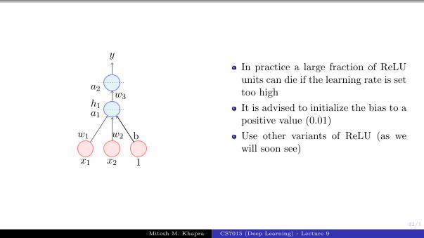
x1 x2 1

y

w1 w2 b

h1a1

a2w3

In practice a large fraction of ReLUunits can die if the learning rate is settoo high

It is advised to initialize the bias to apositive value (0.01)

Use other variants of ReLU (as wewill soon see)


43/1

Leaky ReLU

x

y

f(x) = max(0.01x,x)

No saturation

Will not die (0.01x ensures thatat least a small gradient will flowthrough)

Computationally efficient

Close to zero centered ouputs

Parametric ReLU

f(x) = max(αx, x)

α is a parameter of the model

α will get updated during backpropagation


44/1

Exponential Linear Unit

x

y

f(x) = x if x > 0

= aex − 1 if x ≤ 0

All benefits of ReLU

aex − 1 ensures that at least a smallgradient will flow through

Close to zero centered outputs

Expensive (requires computation ofexp(x))


45/1

Maxout Neuron

max(wT1 x+ b1, wT2 x+ b2)

Generalizes ReLU and Leaky ReLU

No saturation! No death!

Doubles the number of parameters


46/1

Things to Remember

Sigmoids are bad

ReLU is more or less the standard unit for Convolutional Neural Networks

Can explore Leaky ReLU/Maxout/ELU

tanh sigmoids are still used in LSTMs/RNNs (we will see more on this later)


47/1

Module 9.4 : Better initialization strategies


48/1







49/1

y

σ σ σ

σ

x1 x2

h21

a21

h11 h12 h13

a11 a12 a13

a11 = w11x1 + w12x2

a12 = w21x1 + w22x2

∴ a11 = a12 = 0

∴ h11 = h12

What happens if we initialize allweights to 0?

All neurons in layer 1 will get thesame activation

Now what will happen during backpropagation?

∇w11 =∂L (w)

∂y.∂y

∂h11.∂h11∂a11

.x1

∇w21 =∂L (w)

∂y.∂y

∂h12.∂h12∂a12

.x1

but h11 = h12

and a12 = a12

∴ ∇w11 = ∇w21

Hence both the weights will get thesame update and remain equal

Infact this symmetry will never breakduring training

The same is true for w12 and w22

And for all weights in layer 2 (infact,work out the math and convince your-self that all the weights in this layerwill remain equal )

This is known as the symmetrybreaking problem

This will happen if all the weights ina network are initialized to the samevalue


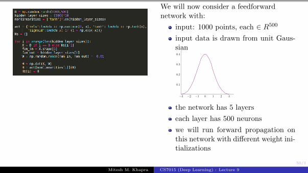
50/1

We will now consider a feedforwardnetwork with:

input: 1000 points, each ∈ R500

input data is drawn from unit Gaus-sian

−3 −2 −1 0 1 2 3

0.1

0.2

0.3

0.4

the network has 5 layers

each layer has 500 neurons

we will run forward propagation onthis network with different weight ini-tializations


51/1

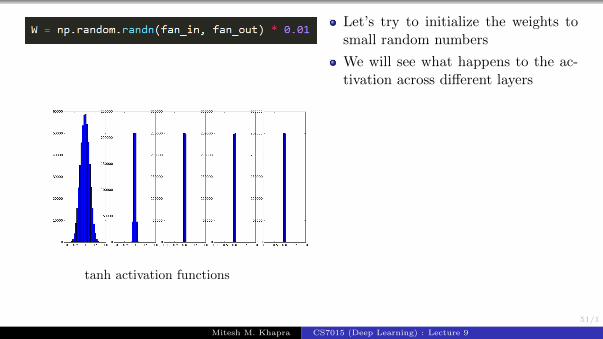
tanh activation functions

sigmoid activation functions

Let’s try to initialize the weights tosmall random numbers

We will see what happens to the ac-tivation across different layers


52/1

What will happen during backpropagation?

Recall that ∇w1 is proportional tothe activation passing through it

If all the activations in a layer arevery close to 0, what will happen tothe gradient of the weights connect-ing this layer to the next layer?

They will all be close to 0 (vanishinggradient problem)


53/1

sigmoid activations with large weights

tanh activation with large weights

Let us try to initialize the weights tolarge random numbers

Most activations have saturated

What happens to the gradients at sat-uration?

They will all be close to 0 (vanishinggradient problem)


54/1

x1 x2 x3

s1ns11

xn

[Assuming 0 Mean inputs andweights]

[Assuming V ar(xi) = V ar(x)∀i ]

[AssumingV ar(w1i) = V ar(w)∀i]

Let us try to arrive at a more principledway of initializing weights

s11 =

n∑i=1

w1ixi

V ar(s11) = V ar(

n∑i=1

w1ixi) =

n∑i=1

V ar(w1ixi)

=

n∑i=1

[(E[w1i])

2V ar(xi)

+ (E[xi])2V ar(w1i) + V ar(xi)V ar(w1i)

]=

n∑i=1

V ar(xi)V ar(w1i)

= (nV ar(w))(V ar(x))


55/1

x1 x2 x3

s1ns11

xn

In general,

V ar(S1i) = (nV ar(w))(V ar(x))

What would happen if nV ar(w) 1?

The variance of S1i will be large

What would happen if nV ar(w)→ 0?

The variance of S1i will be small


56/1

x1 x2 x3

s1ns11

s21

xn

V ar(Si1) = nV ar(w1)V ar(x)

Let us see what happens if we add onemore layer

Using the same procedure as abovewe will arrive at

V ar(s21) =

n∑i=1

V ar(s1i)V ar(w2i)

= nV ar(s1i)V ar(w2)

V ar(s21) ∝ [nV ar(w2)][nV ar(w1)]V ar(x)

∝ [nV ar(w)]2V ar(x)

Assuming weights across all layers

have the same variance


57/1

V ar(az) = a2(V ar(z))

In general,

V ar(ski) = [nV ar(w)]kV ar(x)

To ensure that variance in the output of anylayer does not blow up or shrink we want:

nV ar(w) = 1

If we draw the weights from a unit Gaussianand scale them by 1√

nthen, we have :

nV ar(w) = nV ar(z√n

)

= n ∗ 1

nV ar(z) = 1← (UnitGaussian)


58/1

sigmoid activations

tanh activation

Let’s see what happens if we use thisinitialization


59/1

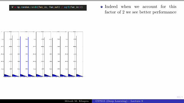
However this does not work for ReLUneurons

Why ?

Intuition: He et.al. argue that afactor of 2 is needed when dealingwith ReLU Neurons

Intuitively this happens because therange of ReLU neurons is restrictedonly to the positive half of the space


60/1

Indeed when we account for thisfactor of 2 we see better performance


61/1

Module 9.5 : Batch Normalization


62/1

We will now see a method called batch normalization which allows us to be lesscareful about initialization


63/1

x1 x2 x3

h0

h1

h2

h3

h4

To understand the intuition behind Batch Nor-malization let us consider a deep network

Let us focus on the learning process for the weightsbetween these two layers

Typically we use mini-batch algorithms

What would happen if there is a constant changein the distribution of h3

In other words what would happen if across mini-batches the distribution of h3 keeps changing

Would the learning process be easy or hard?


64/1

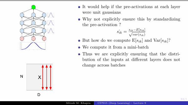
It would help if the pre-activations at each layerwere unit gaussians

Why not explicitly ensure this by standardizingthe pre-activation ?

sik = sik−E[sik]√var(sik)

But how do we compute E[sik] and Var[sik]?

We compute it from a mini-batch

Thus we are explicitly ensuring that the distri-bution of the inputs at different layers does notchange across batches


65/1

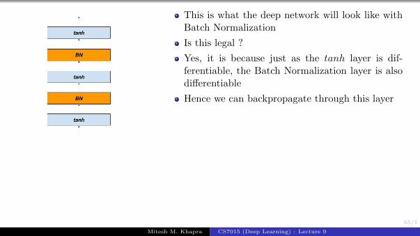
This is what the deep network will look like withBatch Normalization

Is this legal ?

Yes, it is because just as the tanh layer is dif-ferentiable, the Batch Normalization layer is alsodifferentiable

Hence we can backpropagate through this layer


66/1

γk and βk are additionalparameters of the network.

Catch: Do we necessarily want to force a unitgaussian input to the tanh layer?

Why not let the network learn what is best for it?

After the Batch Normalization step add the fol-lowing step:

y(k) = γksik + β(k)

What happens if the network learns:

γk =√var(xk)

βk = E[xk]

We will recover sik

In other words by adjusting these additional para-meters the network can learn to recover sik if thatis more favourable


67/1

We will now compare the performance with and without batch normalization onMNIST data using 2 layers....


68/1


69/1

2016-17: Still exciting times

Even better optimization methods

Data driven initialization methods

Beyond batch normalization


cs7015 (deep learning) : lecture 9miteshk/cs7015/slides/handout/lecture… · mitesh m. khapra...

Documents