cs6604 digital libraries
TRANSCRIPT

CS6604 Digital Libraries
Toward an Intelligent Crawling Scheduler forArchiving News Websites Using Reinforcement
Learning
Authors
Xinyue Wang
Naman Ahuja
Ritesh Bansal
Siddharth Dhar
Nathaniel Llorens
Instructor
Dr. Edward A. Fox
Department of Computer Science
Virginia Tech
Blacksburg, VA 24061
January 16, 2020
CS6604: Digital Libraries, Fall 2019
Team Web Archive: Xinyue Wang, Naman Ahuja, Ritesh Bansal, Siddharth Dhar,
Nathaniel Llorens
https://github.com/xw0078/VT_fall19_cs6604_webarchive
This research was done under the supervision of Dr. Edward A. Fox as part of the course
CS6604: Digital Libraries at Virginia Tech, Fall 2019.
2nd edition, December 30, 2019
Contents
Abstract vi
List of Figures vii
List of Tables ix
1 Introduction 11.1 Overview . . . . . . . . . . . . . . . . . . . . . . . . . . . . . . . . . . . . 1
1.2 Research Questions . . . . . . . . . . . . . . . . . . . . . . . . . . . . . . 3
2 Literature Review 42.1 Related Works . . . . . . . . . . . . . . . . . . . . . . . . . . . . . . . . . 4
2.2 Traditional Methods and Reinforcement Learning . . . . . . . . . . . . . 6
3 Approach and Design 93.1 Problem Formulation . . . . . . . . . . . . . . . . . . . . . . . . . . . . . 9
3.1.1 Types of Web Page Content Change . . . . . . . . . . . . . . . . . 9
3.1.2 Web Site Structure Change . . . . . . . . . . . . . . . . . . . . . . 9
3.1.3 Information Observability . . . . . . . . . . . . . . . . . . . . . . 10
3.2 History Records and Ground Truth . . . . . . . . . . . . . . . . . . . . . 10
3.3 Traditional Supervised Learning . . . . . . . . . . . . . . . . . . . . . . . 10
3.4 Reinforcement Learning . . . . . . . . . . . . . . . . . . . . . . . . . . . . 12
3.5 Experiment Design . . . . . . . . . . . . . . . . . . . . . . . . . . . . . . 12
4 Implementation 144.1 Data Collection . . . . . . . . . . . . . . . . . . . . . . . . . . . . . . . . 14
4.1.1 Web Archive Storage Standards . . . . . . . . . . . . . . . . . . . 14
4.1.2 Archive.org Collection . . . . . . . . . . . . . . . . . . . . . . . . 15
iii
4.1.3 Alternative Way to Get Data from Internet Archive . . . . . . . . 15
4.1.4 Frequent Recent Crawls . . . . . . . . . . . . . . . . . . . . . . . 16
4.1.5 Convert WARC to Parquet . . . . . . . . . . . . . . . . . . . . . . 16
4.2 Find Unique Web Page Copies in the Archive . . . . . . . . . . . . . . . . 17
4.2.1 HTML Tree Similarity . . . . . . . . . . . . . . . . . . . . . . . . 18
4.2.2 Webpage Style Similarity . . . . . . . . . . . . . . . . . . . . . . . 19
4.2.3 Webpage Body Content Similarity . . . . . . . . . . . . . . . . . . 20
4.2.4 Model Web Content Change Baselines . . . . . . . . . . . . . . . 21
4.3 Model Site Map Change in the Archive . . . . . . . . . . . . . . . . . . . 21
4.3.1 Site Map: Tree Structure . . . . . . . . . . . . . . . . . . . . . . . 22
4.3.2 Generating Sitemap . . . . . . . . . . . . . . . . . . . . . . . . . . 23
4.3.3 Matrix Conversion . . . . . . . . . . . . . . . . . . . . . . . . . . 24
4.3.4 Predict Site Crawl - Baseline Models . . . . . . . . . . . . . . . . 24
4.3.5 Visualization . . . . . . . . . . . . . . . . . . . . . . . . . . . . . . 26
4.4 Model Web Page Content Change with Reinforcement Deep Learning . . 26
4.4.1 Environment and Observation Space . . . . . . . . . . . . . . . . 26
4.4.2 Agent, Action, and Reward . . . . . . . . . . . . . . . . . . . . . . 27
4.4.3 Learning Policy . . . . . . . . . . . . . . . . . . . . . . . . . . . . 30
5 Evaluation 325.1 Supervised Learning Baselines . . . . . . . . . . . . . . . . . . . . . . . . 32
5.1.1 Web Content Change . . . . . . . . . . . . . . . . . . . . . . . . . 33
5.1.2 Sitemap Change . . . . . . . . . . . . . . . . . . . . . . . . . . . . 38
5.2 Reinforcement Learning . . . . . . . . . . . . . . . . . . . . . . . . . . . . 42
5.2.1 Future Work . . . . . . . . . . . . . . . . . . . . . . . . . . . . . . 43
5.3 Conclusion . . . . . . . . . . . . . . . . . . . . . . . . . . . . . . . . . . . 44
6 Future Work 456.1 Evaluation . . . . . . . . . . . . . . . . . . . . . . . . . . . . . . . . . . . 45
6.2 Further Baseline Model Design . . . . . . . . . . . . . . . . . . . . . . . . 45
6.3 Further RL Model Design . . . . . . . . . . . . . . . . . . . . . . . . . . . 45
7 Lessons Learned 477.1 Data Pre-processing . . . . . . . . . . . . . . . . . . . . . . . . . . . . . . 47
7.2 Constructing Baselines . . . . . . . . . . . . . . . . . . . . . . . . . . . . 48
iv
7.3 RL model design . . . . . . . . . . . . . . . . . . . . . . . . . . . . . . . . 48
8 Acknowledgements 50
9 User Manual 519.1 ArchiveOrgCollectionScraper . . . . . . . . . . . . . . . . . . . . . . . . . 51
9.2 Zeppelin . . . . . . . . . . . . . . . . . . . . . . . . . . . . . . . . . . . . 51
9.3 Web2Warc . . . . . . . . . . . . . . . . . . . . . . . . . . . . . . . . . . . 52
9.4 Archive Unleashed Toolkit (AUT) . . . . . . . . . . . . . . . . . . . . . . 52
9.5 Heritrix . . . . . . . . . . . . . . . . . . . . . . . . . . . . . . . . . . . . . 52
9.6 HTML-Similarity . . . . . . . . . . . . . . . . . . . . . . . . . . . . . . . 52
9.7 TextDistance . . . . . . . . . . . . . . . . . . . . . . . . . . . . . . . . . . 53
9.8 BeautifulSoup . . . . . . . . . . . . . . . . . . . . . . . . . . . . . . . . . 53
9.9 PySpark . . . . . . . . . . . . . . . . . . . . . . . . . . . . . . . . . . . . . 53
9.10 Prophet . . . . . . . . . . . . . . . . . . . . . . . . . . . . . . . . . . . . . 54
9.11 scikit-learn . . . . . . . . . . . . . . . . . . . . . . . . . . . . . . . . . . . 54
9.12 OpenAI Gym . . . . . . . . . . . . . . . . . . . . . . . . . . . . . . . . . . 54
9.13 Stable Baselines . . . . . . . . . . . . . . . . . . . . . . . . . . . . . . . . 54
10 Developer’s Manual 5510.1 Project Architecture and Inventory . . . . . . . . . . . . . . . . . . . . . 55
10.2 File Inventory . . . . . . . . . . . . . . . . . . . . . . . . . . . . . . . . . 55
10.3 Method Descriptions . . . . . . . . . . . . . . . . . . . . . . . . . . . . . 56
Bibliography 58
Appendix A Project Plan and Calendar 60
v
Abstract
Web crawling is one of the fundamental activities for many kinds of web technology or-
ganizations and companies such as Internet Archive and Google. While companies like
Google often focus on content delivery for users, web archiving organizations such as
the Internet Archive pay more attention to the accurate preservation of the web. Crawl-
ing accuracy and e�ciency are major concerns in this task. An ideal crawling module
should be able to keep up with the changes in the target web site with minimal crawling
frequency to maximize the routine crawling e�ciency. In this project, we investigate us-
ing information from web archives’ history to help the crawling process within the scope
of news websites. We aim to build a smart crawling module that can predict web content
change accurately both on the web page and web site structure level through modern
machine learning algorithms and deep learning architectures.
At the end of the project: We have collected and processed raw web archive col-
lections from Archive.org and through our frequent crawling jobs. We have developed
methods to extract identical copies of web page content and web site structure from the
web archive data. We have implemented baseline models for predicting web page con-
tent change and web site structure change with supervised machine learning algorithms.
We have implemented two di�erent reinforcement learning models for generating a web
page crawling plan: a continuous prediction model and a sparse prediction model. Our
results show that the reinforcement learning modal has the potential to work as an in-
telligent web crawling scheduler.
vi
List of Figures
2.1 SVM’s soft margin formulation [3] . . . . . . . . . . . . . . . . . . . . . . 7
3.1 Di�erent settings of data sources and training/testing design . . . . . . . 11
4.1 Web page viewed as a DOM tree [19] . . . . . . . . . . . . . . . . . . . . 18
4.2 A sample DOM tree with post order numbering for DOM elements [19] . 19
4.3 Various operations on DOM [19] . . . . . . . . . . . . . . . . . . . . . . . 19
4.4 Sample Sitemap in Graph Structure . . . . . . . . . . . . . . . . . . . . . 22
4.5 Sample Ancestor Matrix for a Given Tree Structure . . . . . . . . . . . . 25
4.6 A general view of our proposed reinforcement learning environment for
the web crawling task for one time step: At each time step, the agent will
learn from the historical observation and perform a prede�ned crawling
action. Then the sliding window will move forward and make a new
history observation that includes the previous action. . . . . . . . . . . . 27
4.7 The general idea of the continuous prediction model: The agent learns
from the observation space and makes the binary prediction (crawl/not
crawl) for each time step. After each prediction, the agent moves forward
to the next time step until it reaches the max range, where we consider
a crawling plan has been generated. The target labels are showing the
positions of ground truth in the data sequence. The blue arrows under
the timeline are showing the time step that is marked as crawl and the
result of comparing with ground truth. . . . . . . . . . . . . . . . . . . . 29
4.8 The general idea of the sparse prediction model: The agent learns from
the observation space and predicts with multiple positions for crawling.
The target labels are showing the positions of ground truth in the data
sequence. The blue arrows under the timeline are showing the time step
that is marked as crawl and the compared result with ground truth. . . . 30
vii
5.1 High Level Overview of Supervised Learning architecture . . . . . . . . . 33
5.2 The output of the Facebook Prophet model illustrating the number of
hours elapsed since the last determined change on cnn.com based on the
crawled data. It also shows predictions for the next 48 hours. . . . . . . . 37
5.3 The output of the Facebook Prophet illustrating an instance in the future
when the webpage should be crawled according to the model. . . . . . . 37
5.4 Daily trend of the changes recognised by Facebook Prophet . . . . . . . . 38
5.5 Sitemap: High Level Overview of Supervised Learning Architecture . . . 39
5.6 The output of the Facebook Prophet model illustrating prediction per-
centage. It also shows predictions for the next 48 hours. . . . . . . . . . . 41
5.7 The output of the Facebook Prophet, illustrating general trend in the �rst
case and an instance in the future when the website should be crawled
according to the model, in the second case. . . . . . . . . . . . . . . . . . 42
7.1 An example that shows two training processes. A higher positive reward
score indicates that the model is working towards a potential solution. . 49
viii
List of Tables
4.1 A sample web archive record in Parquet. SURT means Sort-friendly URI
Reordering Transform. . . . . . . . . . . . . . . . . . . . . . . . . . . . . 17
4.2 The general rewarding strategies for continuous prediction and sparse
prediction models. The result type indicates the compared result between
model prediction and ground truth. Negative/positive means we use a
negative or positive �oat value as the reward. Since the sparse predic-
tion model does not generate a “not crawl” decision, the reward is not
applicable and marked as N/A. . . . . . . . . . . . . . . . . . . . . . . . . 28
4.3 The score implementations for the rewarding strategies. . . . . . . . . . . 31
5.1 Model Evaluation . . . . . . . . . . . . . . . . . . . . . . . . . . . . . . . 36
5.2 Model Evaluation: Sitemap Classi�cation . . . . . . . . . . . . . . . . . . 41
5.3 The results for RL modal preliminary evaluation. The max score is show-
ing the maximum score the modal could achieve in each plan generation.
The score for each model is the averaged score on the testing data set. . . 43
ix
Chapter 1
Introduction
1.1 Overview
Web archives preserve the content of the current World Wide Web for future use. The
Web is growing rapidly, but so too is information frequently disappearing from the
WWW. In 1997, the founder of the Internet Archive stated that the average lifetime for
a URL was 44 days [8]. In 2001, a study showed that 47% of the web pages became in-
accessible within two years [1]. In 2012, another study stated that about 11 percent of
resources shared online are lost, and that they continue to disappear at a rate of 0.02
percent per day [15]. We do not know how many parts of the WWW are vanishing right
now, but expect the situation to be similar.
The act of preserving the WWW is crucial to record the history of human society.
For this reason, a growing number of memory/heritage institutions actively engage in
web archive activities, e.g., Internet Archive, Common Crawl, and Library of Congress.
Though various institutions are dedicated to web archive activities, many of them are
non-pro�t corporations. Due to limitations in resources available, it would be helpful to
have ways to improve their crawling accuracy and e�ciency.
The essential activity of preserving the WWW is crawling, e.g., of known web sites
or web pages, as well as new ones as they appear. The existing crawling model in the web
archive communities mainly adopts prede�ned crawling criteria for corresponding can-
didates, which are usually managed by human coordinators. As an example, at Virginia
Tech, the University Library works with Archive-It, a web archive crawling system from
the Internet Archive, for routine preservation of the Virginia Tech domain (vt.edu). The
1
following list gives some details about how the Virginia Tech library set up the crawling
policies:
• Crawls are managed by the Digital Preservation Coordinator.
• Crawls are performed biannually and as needed.
• The scope of the crawl searches for hyperlinks four levels from the original seed.
• Requests for adding a seed to the Web Archive can be directed to the Digital Preser-
vation Coordinator.
This typical example shows that the crawling policy is often designed with a �xed
frequency and a certain level of hyperlinks to be discovered. For preservers that are
familiar with their collection, these rules could potentially capture most of the changes
as desired with proper resources dedicated to the purpose.
Besides user-de�ned special collections, the other major part of web archive activity
is the general crawling over the internet, a principal activity of search engine companies
like Google or Microsoft. In general, more frequent crawls will lead to better accuracy.
At the same time, more frequent crawls also could waste computational resources if oc-
curring beyond the web change frequency. Accordingly, general crawls usually adopt
dynamic rules to adapt to web site behavior. Di�erent kinds of web sites behave di�er-
ently: social network web sites often change dynamically and could change every second;
News websites could be updated every hour. Further, more news often leads to more web
pages within the site. Information resources like wikis are continually changing based on
the user behavior. These examples show that Web sites in di�erent categories should be
looked at di�erently when modeling their changing behavior. Through suitable model-
ing, the changing behavior of web sites can lead to a better crawling process that decides
when the crawler should revisit the web site or page and so keeps up with all the changes.
In our project, we focus on the problem of modeling the changing behavior of news
web sites such as CNN and ABC. We propose to build a model that can learn the historical
information from web archives about the news web page/site change behavior, and use
the model to predict future web changes as an indicator for a crawling scheduler to cover
potential new information. We speci�cally explore reinforcement learning algorithms to
solve our problem. We compare the result of our approach with existing methods.
2

1.2 Research Questions
This project addresses problems related to modeling news web page/site changes for
crawling scheduling by answering the following research questions:
RQ1: Can we automatically and e�ectively identify the unique copies of a web page in anews website from its archive?
RQ2: Can we automatically and e�ectively identify the unique site structure of a newswebsite from its archive?
RQ3: Can we use the archived information for future web page/site change prediction?
RQ4: Can a deep learning model through reinforcement learning techniques surpass theexisting methods on predicting the future changes of a web page/site?
3
Chapter 2
Literature Review
2.1 Related Works
Radinsky [13] introduces a traditional machine-learning-based approach to predicting
web page content change. Two types of information observability scenarios are de�ned
in this paper for the general web page content prediction problem: fully-observed and
partially-observed. This paper focuses on the fully-observed scenario, which means the
past histories that will be used for future predictions are all observed, but in our project,
we cover both scenarios. The author designed the approach of predicting web page con-
tent change as a classi�cation problem where each candidate page is assessed daily to
determine if it should be crawled. The primary goal of the paper is to determine the ef-
fectiveness of a list of prede�ned features, so the same SVM algorithm is applied for all of
the experiments. Three types of features are introduced as an information source: page
changing frequency (1D), various page content (2D), and related pages content (3D). The
result shows that 3D features lead to the best performance on the task, and 2D is better
than 1D. This paper shows that the machine-learning-based approach is promising for
this problem. In our project, we propose to expand this idea to deep learning and combine
it with web archive data.
In Using Visual Pages Analysis for OptimizingWeb Archiving [14], Saad et al. provide a
procedure for determining the interval to crawl a certain pre-speci�ed set of web pages.
Speci�cally, they intend to provide information to two types of crawlers: a crawler that
crawls on a speci�ed interval, and a crawler that crawls the least fresh page as determined
by a scheduler. The approach uses visual analysis and machine learning to break a web
4

page into its component blocks, and then compares between archived versions of the web
page to determine if blocks deemed important by the algorithm often change in the page.
If they do, the page is prioritized for crawling, but if not the priority might be lowered
on the stack. The speci�cs of how this is done includes processing a web page into a
format similar to XML and then using XML di�erentiating software to �nd the changes
and put them into a new XML �le containing the deltas. The purpose of this research
is to avoid crawling web pages that do not change or have unimportant changes like
advertisements that refresh constantly. This paper stood out to us because it suggests a
method that we could consider in our goal of �nding the di�erences between web pages
in order to predict the optimal crawler scheduling.
Gowda and Mattmann [4] consider clustering web pages based on various techniques
to group the pages. They focus on clustering based on the web page structure and style
for applications like categorization, cleaning, schema detection, and automatic extrac-
tion. This can be really useful for our task of di�erentiating web pages on the basis of
HTML similarity. The structural similarity of HTML pages is measured by using the Tree
Edit Distance measure on DOM trees. The stylistic similarity is measured by using Jac-
card similarity on CSS class names. An aggregated similarity measure is computed by
combining structural and stylistic measures. We incorporate the syntactic dissimilarity
by computing the tree di�erence, CSS classes di�erence, and the aggregate di�erence to
di�erentiate the web pages.
Meegahapola et al. [10] propose a methodology to detect the frequency of change in
web pages to optimize server-side scheduling of change detection and noti�cation sys-
tems. The proposed method is based on a dynamic detection process, where the crawling
schedule will be adjusted accordingly in order to result in a more e�cient server-based
scheduler to detect changes in web pages.
Law [9] tries to build an e�cient page comparison system by comparing the struc-
tural and visual features of the web pages. The structural comparison is used to �nd
dissimilarities in case di�erent scripts are rendering the same content or if there is a
change in hyperlinks. Visual comparison can �nd dissimilarities if the code of the web
page was unchanged but an image being loaded was updated. They propose a hybrid web
page comparison framework that combines the structural and visual comparison meth-
ods. They additionally propose machine learning that sets all the similarity parameters
and combination weights.
Pehlivan and Saad [12] address the problem of understanding what happened betweentwo versions of a web page. Most of the web pages on the internet are HTML, but HTML is
5
considered to be semantically poor. Comparing two versions of HTML web pages based
on the DOM tree does not provide relevant information that will help us to understand
the changes. They propose a change detection approach that computes the semantic
di�erences between two versions of a web page by detecting changes in the visual rep-
resentation of the two versions. The visual aspect provides an insight into the semantic
structure of the document.The proposed approach, Vi-DIFF, compares the two versions
of a web page in three steps.
1. Segmentation: Partition the web page into visual semantic blocks.
2. Change Detection: Compare the two restructured versions of the web pages.
3. Delta File Generation: Produce a �le describing the visual changes.
They also introduce a new change detection algorithm, that is used in step 2, that
takes into account the structure of the web page while comparing.
Yang and Song [18] propose a new method to extract the text content from web pages
to overcome the limitations of the traditional techniques. Those are successfully able
to remove invisible noise like styles, comments, and scripts but they still leave behind
a large portion of the visible noise that includes navigation links, sidebars, copyright
statements, etc. that lead to lower accuracy of the text extraction algorithm. In their
proposed approach, they remove not just the invisible noise but also the visible noise, to
a large extent. This results in more pure web pages for content extraction. Then they
utilize the relationships between text length, punctuation, and links to extract the web
page text.
Taylor and Letham [17] address the challenges associated with producing reliable
and high quality forecasts from a variety of time series data. They describe a practical
approach to forecasting “at scale” that combines con�gurable models with analyst-in-the-
loop performance analysis. They propose a modular regression model with interpretable
parameters that can be intuitively adjusted by analysts with domain knowledge about
the time series.
2.2 Traditional Methods and Reinforcement Learning
A Support Vector Machine (SVM) is a discriminative classi�er formally de�ned by a sepa-
rating hyperplane. It is a non-probabilistic binary linear classi�er that analyzes data used
for classi�cation and regression analysis. SVMs can be used to solve various real-world
problems. They are helpful in text and hypertext categorization, as their application can
6
signi�cantly reduce the need for labelled training instances in both the standard inductive
and transductive settings. Classi�cation of images can also be performed using SVMs.
Experimental results show that SVMs achieve signi�cantly higher search accuracy than
traditional query re�nement schemes after just three to four rounds of relevance feed-
back.
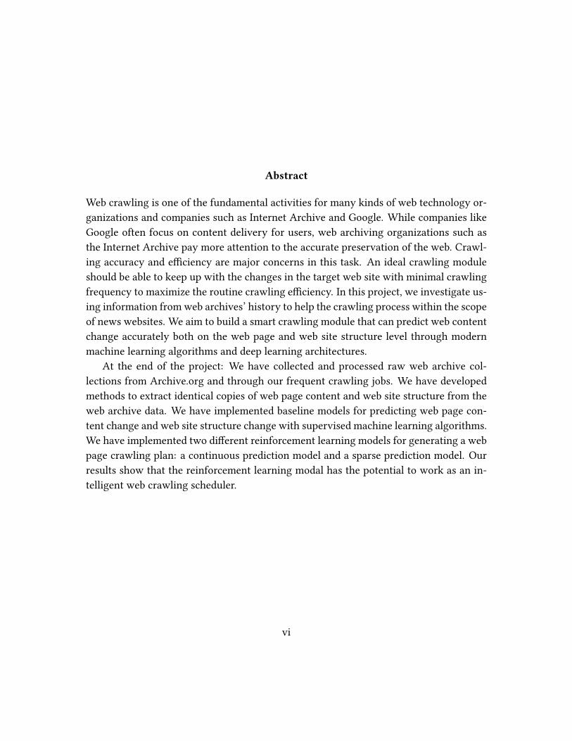
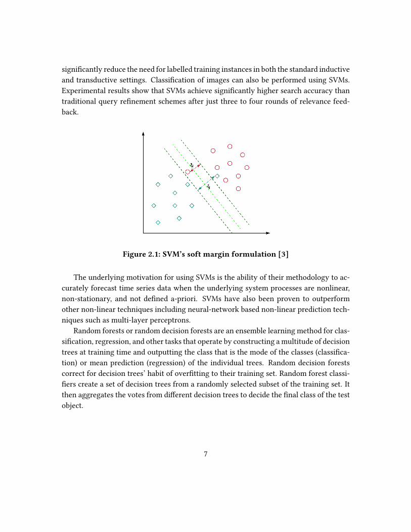
Figure 2.1: SVM’s soft margin formulation [3]
The underlying motivation for using SVMs is the ability of their methodology to ac-
curately forecast time series data when the underlying system processes are nonlinear,
non-stationary, and not de�ned a-priori. SVMs have also been proven to outperform
other non-linear techniques including neural-network based non-linear prediction tech-
niques such as multi-layer perceptrons.
Random forests or random decision forests are an ensemble learning method for clas-
si�cation, regression, and other tasks that operate by constructing a multitude of decision
trees at training time and outputting the class that is the mode of the classes (classi�ca-
tion) or mean prediction (regression) of the individual trees. Random decision forests
correct for decision trees’ habit of over�tting to their training set. Random forest classi-
�ers create a set of decision trees from a randomly selected subset of the training set. It
then aggregates the votes from di�erent decision trees to decide the �nal class of the test
object.
7
Facebook Prophet uses a decomposable time series model [5] with three main model
components: trend, seasonality, and holidays. They are combined in the following equa-
tion:
y(t) = д(t) + s(t) + h(t) + ϵt (2.1)
Here g(t) is the trend function which models non-periodic changes in the value of
the time series, s(t) represents periodic changes (e.g., weekly and yearly seasonality), and
h(t) represents the e�ects of holidays which occur on potentially irregular schedules over
one or more days. The error term ϵt represents any idiosyncratic changes which are not
accommodated by the model. This speci�cation is similar to a generalized additive model
(GAM) [6], a class of regression models with potentially non-linear smoothers applied to
the regressors. Here only time as a regressor is used. Modelling seasonality as an additive
component is the same approach taken by exponential smoothing.
So far, we have covered several methods on how to model web site content change
in a traditional supervised machine learning setting: the problem is essentially modeled
as a time series prediction problem. These methods focus on the prediction of when or
whether the web would change at a speci�c time in the future. After that, the prediction
results can be used as an indicator to help the crawling scheduler to make plans and
actions.
In this project, instead of traditional supervised learning, we propose to use rein-
forcement learning to solve the crawling prediction problem. Reinforcement learning is
widely used in robotics or game AI where the model can learn to make optimal decisions
to reach the goal based on given environment. Traditionally, RL model is not a good
approach for time-series forecasting problems since RL model focuses on optimizing fu-
ture outcomes instead of future events. Here, we want to convert the traditional time
series prediction scenario to an environment that can �t RL model: Instead of predicting
the future changes of web page changes as an intermediate step, we directly look at the
crawling decisions as the output of the model. In this case, the RL model will learn to
make crawling decisions based on the time-series web history data (environment). With
this approach, we expect the RL model to handle two important parts of the problem at
the same time: predicting the future behavior of web page change (the same problem as
in supervised learning model) and making crawling decisions.
8

Chapter 3
Approach and Design
3.1 Problem Formulation
Focusing on news web sites, we investigate the possibility of estimating web page con-
tent change and web site structure change through reinforcement deep learning under a
partially observed information history. We take web archive history as the source of his-
torical data and use the information to predict future changes, which can be used by a web
crawling scheduler to make better crawl plans. Under the traditional supervised learning
setting, the model will try to predict the state of web content based on the archived his-
torical information: whether a signi�cant change will happen at a particular time. Under
the reinforcement learning setting, the model itself will simulate a web crawler and try
to make optimal crawling plans given the history of the web content.
3.1.1 Types of Web Page Content Change
There are di�erent types of web page content change: the publisher changes the web
page content; the web page can be changed through user interaction; and the web page
changes based on the browsing user pro�le. In our project, we mainly focus on the type
where the publisher changes the page.
3.1.2 Web Site Structure Change
We consider the web site structure in a tree representation. Each page represents one
node on the tree; the home page is the root node. We consider two types of web page
9
structure change: disappearing node, which means a particular page is removed from the
web site; and new node, which means a new page is added to the web site.
3.1.3 Information Observability
Radinsky’s work [13] introduces two di�erent observability scenarios for the web page
histories: (1) in a fully-observed scenario, all the history of a web page that will be used
as information source is available; and (2) in a partially-observed scenario, only a partial
history of the web pages is available. In reality, the partially-observed scenario is a typical
case. For the type of web page change that is driven by a publisher, we can determine
the observability for a page or website through its crawling policy, which means if the
policy maker can guarantee the accuracy of the policy based on domain knowledge.
In our project, we investigate both observability scenarios. As a fully-observed sce-
nario has been con�rmed to be valid on this task, we explore the possibility of using
partially-observed histories to achieve the same goal.
3.2 History Records and Ground Truth
The main goal of the project is to discover the possibility of using historical web archive
information to predict the future behavior of the web page content, including web pages
and web site structures. We plan to gather the web archive collection from Archive.org
as part of our historical records. We then set up a frequently enough crawling for the
same set of archival records, which can be seen as the ground truth for the web content
behavior over time. The historical records will be used as our training dataset for the
model and the ground truth will be used to test the performance of our model.
3.3 Traditional Supervised Learning
Our goal is to predict web content change using the crawled time series data. Using this
data, we will predict the future changes to web content by re-framing the problem as a
classi�cation and a regression task.
We will form a series of inputs and corresponding labels for the classi�cation problem
using SVM and Random Forest. We will also use Facebook Prophet to forecast the future
value using the input time series data. Prophet is a procedure for forecasting time series
10
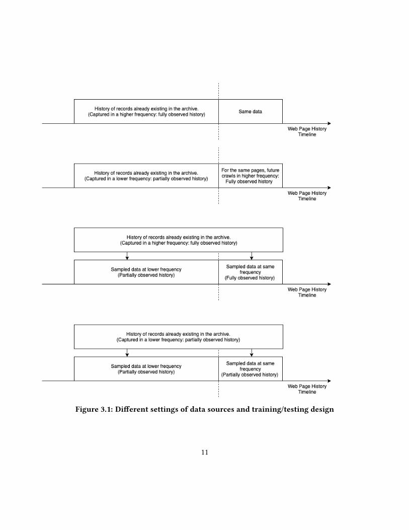
Figure 3.1: Di�erent settings of data sources and training/testing design
11
data based on an additive model where non-linear trends are �t with yearly, weekly,
and daily seasonality. It is robust to missing data and shifts in the trends, and typically
handles outliers well. We will cover a detailed description of data processing needed for
the tasks and their implementations in later sections.
3.4 Reinforcement Learning
The nature of our goal, predicting web content change, can be generally considered as
a time series prediction problem, which is a good �t with a supervised machine learn-
ing problem. However, usually, reinforcement learning is not a good option to perform
prediction tasks with time series data. So, why would we want to apply reinforcement
learning to such a problem? To answer this question, we need to go back to our original
motivation: create a better crawling scheduler. The prediction part is derived out of the
original goal and it can be generally considered as the fundamental part, that can help
to make the crawler smarter. Instead of focusing on the prediction task, reinforcement
learning can directly model the crawling scheduler to achieve the original goal: we are
going to train the agent to be capable of making optimal crawling plans in our de�ned
environment. In this case, the prediction problem can be considered as a hidden task for
the reinforcement learning model to be considered, and the model would use this infor-
mation to make optimal decisions. We will discuss two di�erent crawling strategies for
the reinforcement learning in section 4.4.
3.5 Experiment Design
We follow the steps shown below:
1. Set up a crawler for the news website with a frequent policy which can guarantee
the collection of a fully-observed history.
2. Collect the same news website data from the Internet Archive with a longer history.
3. Validate the observability of archived data.
4. Identify the unique copies of web pages for each URL in the web archive through
prede�ned criteria.
12

5. Generate the unique site structure for each web site as a time series.
6. Implement baseline methods for web page content change prediction and web site
structure change prediction.
7. Design a reinforcement-learning model for web page content change prediction
and web site structure change prediction.
8. Compare the reinforcement-learning and baseline models.
13
Chapter 4
Implementation
4.1 Data Collection
For this research, our data source comes from Archive.org and our own crawling jobs. We
aim to include the following major news websites in our experiment: CNN, Dailymail,
NYT, FOX, and ABC. In the following parts, we will talk about the web archive data
standards, tools that we used for crawling, description of our desired data, and data pre-
processing.
4.1.1 Web Archive Storage Standards
WARC is the standard �le format used by web archives for long-term preservation.
WARC is a container format to serialize HTTP transactional metadata and payloads.
The full WARC standard information can be found at: https://iipc.github.io/warc-
speci�cations/speci�cations/warc-format/warc-1.0/. We get WARC data from multiple
sources, including Archive.org and the Web2Warc crawler. As WARC is primarily de-
signed for long-term preservation purposes rather than e�ciency in computational pro-
cessing, we will explain in a later section how we convert WARC to the Parquet format
for our research and analysis purposes.
CDX is the common �le format that is used by the web archive community as a sep-
arate index information source for WARC. A CDX �le consists of individual lines of text,
each of which summarizes a single web record in WARC. There are many parts of the
CDX standard that include di�erent types of information. A full CDX data speci�cation
can be found at: https://archive.org/web/researcher/cdx_legend.php. In this project, we
14
do not use CDX �les as our information source. Instead, we integrate the same index
information in the Parquet format to have an aggregated information source to perform
analysis tasks.
4.1.2 Archive.org Collection
Archive.org is the website where Internet Archive hosts most of its web archive collec-
tions. In this project, we include the following collections:
1. https://archive.org/details/cnn.com
2. https://archive.org/details/dailymail.co.uk
3. https://archive.org/details/nytimes.com
4. https://archive.org/details/foxnews.com
5. https://archive.org/details/abcnews.go.com
In Archive.org, each collection contains multiple items that represent multiple types
of crawled data. In each item, the data is preserved in multiple WARC/CDX �les and
related information. Each WARC �le is typically around 1 GB in size. We implement
ArchiveOrgCollectionScraper, a web scraping tool to fetch all the downloadable links for
WARC and CDX �les in the collection. We then use the Wget tool in Linux to download all
of the �les. As a result, we have a collection of Archive.org CNN focus crawls from May
2019 to Oct 2019. We haven’t collected from all of the other news web archive collections
due to storage space limitations. This is planned to be resolved in future research.
Note: Be aware that all the above collections are not public, but we are granted per-
mission to access the data by the Internet Archive, our partner in the NSF-funded collab-
orative research project GETAR.
4.1.3 Alternative Way to Get Data from Internet Archive
Many collections on Archive.org are not public. Even without explicit permission from
the Internet Archive, researchers can use ArchiveSpark to crawl the Wayback Machine
to get desired data since most of the records accessible through the Wayback Machine
are public. ArchiveSpark allows use of a speci�ed URL or domain list for fetching the
15
records from the Wayback Machine within a de�ned period. An example usage can be
found through ArchiveSpark’s documentation at:
https://github.com/helgeho/ArchiveSpark/blob/master/notebooks/Downloading_
WARC_from_Wayback.ipynb
4.1.4 Frequent Recent Crawls
As an addition to the collection from Archive.org, we build our own frequent crawled
collection as the ground truth for our study. Web2Warc is a simple crawler written in
Scala which can generate WARC and CDX output. We use a modi�ed Web2Warc version
for our frequent crawl tasks in this project. For each news web site, we set up a repeating
task to crawl two levels of the domain starting from the landing page. The periodicity
of our crawl is 1 hour. As a result, we have collected data for all 5 news web site from
November 6th to December 1st.
At the beginning, we intended to keep our crawling results consistent with the collec-
tions we get from the Internet Archive. In this case, Heritrix is the best choice. Heritrix
is the Internet Archive’s open-source web crawler that is used for IA’s regular crawling
task. However, we did not get Heritrix working correctly for our purposes. We think this
should be further studied in the future since Heritrix has capability, with �exibility and
multiple functions, to perform crawls with complex rules.
4.1.5 Convert WARC to Parquet
The existing tools for WARC manipulation are limited and not �exible. Thus, we convert
WARC �les to Parquet �les for further experiments. Apache Parquet is a columnar stor-
age format that is designed for e�cient processing and storage. We choose Parquet for
its:
1. columnar representation with intuitive index schema;
2. e�cient searching and �ltering process over index columns;
3. ease of manipulation with most programming languages; and
4. strong support in the Apache Spark framework for big data processing.
16
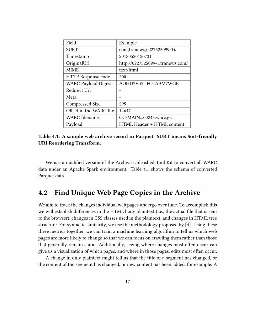
Field Example
SURT com,tranews,0227525099-1)/
Timestamp 20180520120731
OriginalUrl http://0227525099-1.tranews.com/
MIME text/html
HTTP Response code 200
WARC Payload Digest AOHD7VS5...FO4ABM7WGE
Redirect Url -
Meta -
Compressed Size 295
O�set in the WARC �le 14647
WARC �lename CC-MAIN...00245.warc.gz
Payload HTML Header + HTML content
Table 4.1: A sample web archive record in Parquet. SURT means Sort-friendlyURI Reordering Transform.
We use a modi�ed version of the Archive Unleashed Tool Kit to convert all WARC
data under an Apache Spark environment. Table 4.1 shows the schema of converted
Parquet data.
4.2 Find Unique Web Page Copies in the Archive
We aim to track the changes individual web pages undergo over time. To accomplish this
we will establish di�erences in the HTML body plaintext (i.e., the actual �le that is sent
to the browser), changes in CSS classes used in the plaintext, and changes in HTML tree
structure. For syntactic similarity, we use the methodology proposed by [4]. Using these
three metrics together, we can train a machine learning algorithm to tell us which web
pages are more likely to change so that we can focus on crawling them rather than those
that generally remain static. Additionally, seeing where changes most often occur can
give us a visualization of which pages, and where in those pages, edits most often occur.
A change in only plaintext might tell us that the title of a segment has changed, or
the content of the segment has changed, or new content has been added, for example. A
17
change in CSS shows style changes, such as di�erent fonts, colors, or formatting used,
but may not necessarily signal a content change. Lastly, a change in HTML tree structure
could be an indicator of either of the above changes. If new content is added or old
content is deleted, the tree would change. Similarly, if a CSS class that is used changes,
at least the tree node names would change correspondingly. The reason we choose these
three metrics, rather than just one, is that a web page can change in a variety of ways.
There are some web pages where the HTML body never changes, but the JavaScript or
Flash script that governs the dynamic parts of it does. Or, take for example a page whose
HTML body and scripts only change based on input from the backend of a website, like
a realtime stock observer. Finding changes in all three of the aforementioned areas helps
eliminate the possibility of us missing or overstating web page changes.
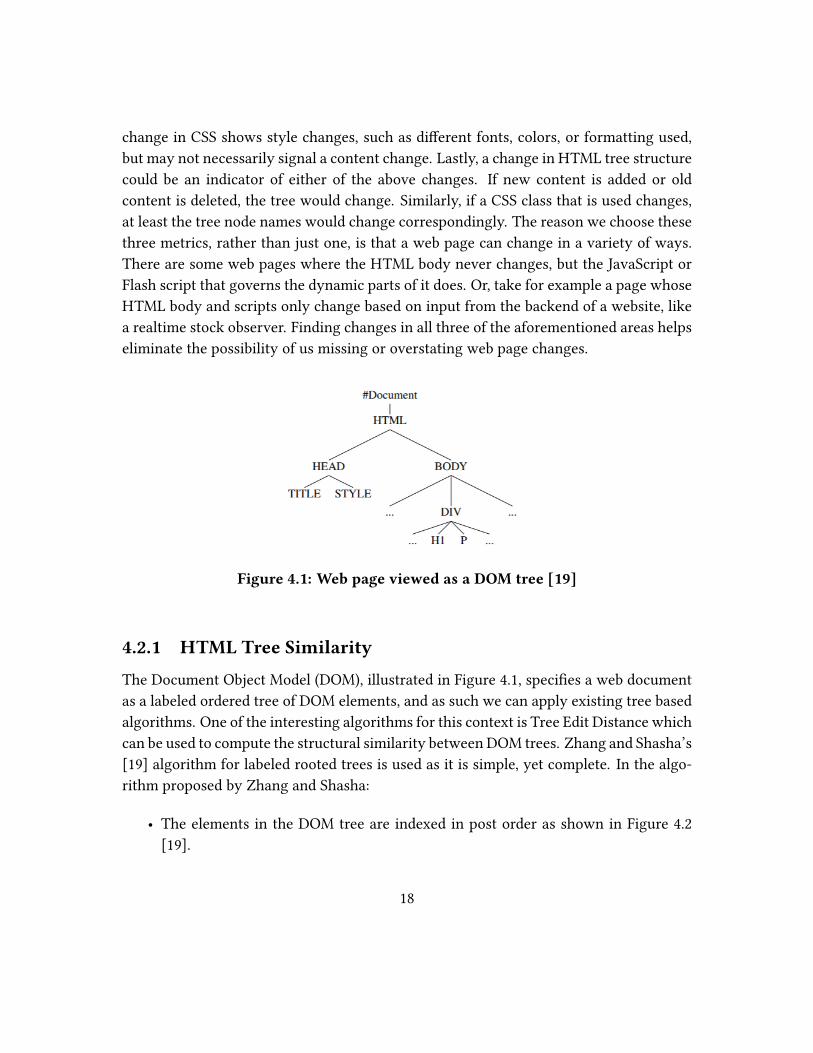
Figure 4.1: Web page viewed as a DOM tree [19]
4.2.1 HTML Tree Similarity
The Document Object Model (DOM), illustrated in Figure 4.1, speci�es a web document
as a labeled ordered tree of DOM elements, and as such we can apply existing tree based
algorithms. One of the interesting algorithms for this context is Tree Edit Distance which
can be used to compute the structural similarity between DOM trees. Zhang and Shasha’s
[19] algorithm for labeled rooted trees is used as it is simple, yet complete. In the algo-
rithm proposed by Zhang and Shasha:
• The elements in the DOM tree are indexed in post order as shown in Figure 4.2
[19].
18
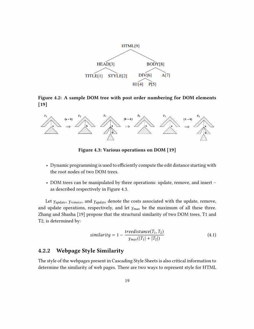
Figure 4.2: A sample DOM tree with post order numbering for DOM elements[19]
Figure 4.3: Various operations on DOM [19]
• Dynamic programming is used to e�ciently compute the edit distance starting with
the root nodes of two DOM trees.
• DOM trees can be manipulated by three operations: update, remove, and insert –
as described respectively in Figure 4.3.
Let γupdate , γremove , and γupdate denote the costs associated with the update, remove,
and update operations, respectively, and let γmax be the maximum of all these three.
Zhang and Shasha [19] propose that the structural similarity of two DOM trees, T1 and
T2, is determined by:
similarity = 1 −treedistance(T1,T2)
γmax (|T1 | + |T2 |)(4.1)
4.2.2 Webpage Style Similarity
The style of the webpages present in Cascading Style Sheets is also critical information to
determine the similarity of web pages. There are two ways to represent style for HTML
19
documents: CSS classes and inline styles. We limit the scope of determining changes on
the basis of CSS classes only. Let A and B be two web pages, and SA and SB represent
the set of CSS classes in A and B, respectively. Jaccard similarity can be used to compute
stylistic di�erences between the two.
SA = classes(A)
SB = classes(B)
style − similarity =|A ∩ B |
|A| + |B | − |A ∩ B |
(4.2)
4.2.3 Webpage Body Content Similarity
To determine text similarity we �rst extract the plaintext from a web page using Beautiful
Soup. We extract the text from all tags in the HTML code except for the script, head, title,
style, and meta tags. Beautiful Soup then strips the HTML tags from the content within
the remaining tags and gives us all the text that is visible on the webpage.
Once we have the plaintext from the two web pages to be compared, we �rst �lter
out the stopwords from the extracted texts and then perform lexical similarity checks
to calculate the similarity between the text content of the web pages. We remove the
stopwords to get a better representation of the similarity, since having the stopwords in
the text will lead to an unnecessarily large number of words in the intersection set of the
two texts and result in a higher similarity value. We perform lexical similarity checks
instead of semantic similarity because we need to check if there is any di�erence in the
actual text content of the web pages rather than the meanings of the content, and lexical
similarity analysis provides a better measure for this.
Jaccard similarity is one method to perform lexical text similarity analysis. In simple
terms, Jaccard similarity is the ratio of the Intersection and the Union of the two texts.
Jaccard Similarity =|TextA ∩TextB |
|TextA ∪TextB |(4.3)
Another similarity measure is the Cosine Similarity. It essentially measures the cosine
of the angle between the vectors generated by the two texts. The vectors are generated
based on the counts of the word tokens in each of the texts. Two similarly oriented vectors
20
will yield a cosine similarity of 1, while two vectors that are oriented at 90 degrees will
yield a cosine similarity of 0.
Cosine Similarity =TextA ·TextB| |TextA | | · | |TextB | |
(4.4)
Edit Distance is used to get a numerical measure of the di�erences between two texts
by counting the minimum number of operations (additions, substitutions, and deletions)
that have to be performed to transform one string to another.
Sorensen-Dice similarity is another similarity measure that can be used to measure
text similarity.
Sorensen − Dice Similarity =2 · |TextA ∩TextB |
|TextA | + |TextB |(4.5)
4.2.4 Model Web Content Change Baselines
We had to pre-process the data from the Parquet �les into a suitable format that could be
provided as an input to the machine learning models. The dataset we created contained
the crawled payloads for a particular web page along with the timestamps of when the
crawls occurred. We will discuss this process in detail in section 5.1.
For our tests, we focused speci�cally on modelling and predicting the change trends
on the cnn.com homepage. This was because our model needed to predict the change
trends on a speci�c web page at a particular time. Further, it was reasonable to assume
that the homepage of the new website cnn.com would be the most frequently changing
page. We believed that this would be the best web page to try out our approach on, and
thus decided to work on just the cnn.com homepage.
4.3 Model Site Map Change in the Archive
Along with detecting page-level changes, we want our model to learn to identify regions
within the structure of the site, which are prone to changes, and to target them �rst. We
also want to make predictions if the crawler should crawl the whole website, signifying
that there is a signi�cant change in the site. To do that, we want to use a sitemap. A
website is a combination of several web pages under a single domain, and the sitemap
characterizes the site.
21
4.3.1 Site Map: Tree Structure
We aim to construct this framework in terms of a tree structure that will represent the
site. The root will represent the homepage, and the nodes will represent the pages of that
site. In essence, from the URLs we have in the archive, we will reconstruct, to the best
of our ability, the tree structure of the actual web site. Unfortunately, it is possible that
we will leave many pages out, since the web crawler only crawls into the web site to a
certain depth, but we expect to at least map most of the higher level pages.
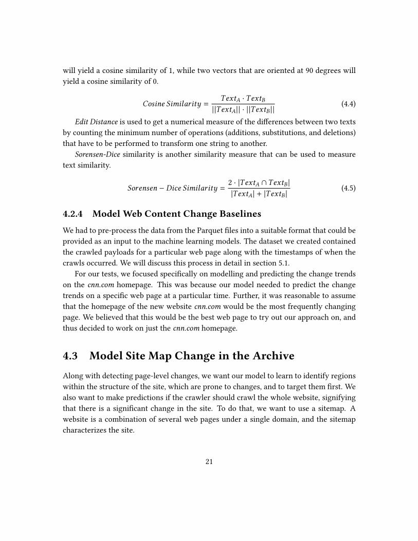
In order to aid the page level comparison, we are also planning to create a timeline
type structure in each node. Each node will contain the page data of that node in a
chronological order, i.e., the �rst timestamp will represent the �rst time that page was
crawled, and the last timestamp will show the latest. This will help us to compare and
visualize the sitemap in di�erent time ranges as well as what parts of a website change
the most or least frequently. Figure 4.4 shows a sample graph structure of such a sitemap.
Figure 4.4: Sample Sitemap in Graph Structure
22
Changes in site structure could tell us where pages are being added or deleted, for
example, giving valuable information on which areas of a web site are receiving the most
modi�cation. In a news website, for instance, we would expect to �nd that the folders or
nodes designated for editorials and articles change the most frequently, as new content
is added every day, and old content is moved to an archive. It would tell us nothing about
how individual pages are changing; rather, it would a�ord us a ‘big picture’ view of the
changes the site undergoes.
4.3.2 Generating Sitemap
Assembling the sitemap will require processing archive data and parsing every URL
crawled, creating a new tree for each new domain. We �nd and assign children to
nodes based on their placement in the URL structure. For example, in a URL such as
www.google.com/drive we will �rst create a tree for the google.com domain, assign the
root node as google.com, and then create a child node of the root named drive. If next we
come across www.google.com/mail, we will add another child node to the root google.comnode named mail. To perform this step, working with the archive data requires some
more �ltering. We only need the media type data among the data crawled; we also check
for status-code, it should be ‘200.’ After �ltering data, we will work towards building the
sitemap. A ‘URL’ consists of hostname, path, and query. To construct the sitemap, we
require the use of hostname and path; the former will act as the root node, and the path
will be used to build up nodes of the hostname. We will also be requiring timestamp and
payload, as the node is expected to be updated with the latest payload and timestamp.
Payloads, saved chronologically, will be used by page-level prediction. The timestamp
and payload received from the archive data are not in the format to be handled and used
by the model. It requires some �ltering, to be rendered usable by the model. Payload
data saved in archive data consists of the HTTP response and page HTML data. We need
to extract that HTML data from the payload and save/use it at the respective node in a
tree structure. This process needs to be repeated for each URL, and once done, the site
map will be created. There will arise a situation where multiple crawls will bring di�er-
ent payloads for the same URL but at di�erent times. In our current implementation, we
are saving these payloads mapped with the timestamp. This implementation will help
perform page-level change detection.
There are additional functionalities that need to be implemented to supplement the
sitemap representation. The �rst one is a sitemap extractor, which is used to extract a sub-
23
sitemap, which takes time range as input and provides a sitemap for that speci�c time. It
will be used to build a matrix of a sitemap, which will act as input to a machine learning
model. Next is a compactor, which is used to compare two sitemaps and help evaluate if
sitemaps were identical. The last one is a matrix generator. These features were created
with the idea in mind that when a machine learning model is created, these supplemental
functionalities will be used to build additional features. Some of these features we thought
of were: (1) sitemap (in matrix form) and (2) site map change binary indicator from last
crawled event (either one or zero). Next, the matrix conversion is described in detail.
4.3.3 Matrix Conversion
To use this feature of detecting change at the site map level in a machine learning model,
we aim to convert a tree structure into a matrix form. This matrix form will preserve
the parent-child relationship of the sitemap and help the model to learn the same. For
this, we are currently exploring the use of the ancestor matrix. An ancestor matrix is a
Boolean matrix, whose cell (i, j) is true if i is an ancestor of j in the tree. The idea is to
traverse the tree in preorder fashion and keep track of ancestors in a container such as
a set, a vector, or an array. Figure 4.5 represents the sample of a ancestor matrix and its
corresponding tree1.
Since we are dealing with time-series data, our approach is to build the sitemap for
intervals and feed it to the machine learning model. The idea behind this is, as time
progresses, changes in site structure will happen, and we will capture these changes in
the matrix, and the machine learning model will be able to learn those changes and so
learn the change pattern.
4.3.4 Predict Site Crawl - Baseline Models
As stated in previous sections, when data from the WARC �le is processed to convert
into the format shown in Table 4.1, we require further pre-processing to build a sitemap
tree structure. It involves using Timestamp, OriginalUrl, MIME, and payload from the
schema. It also should be noted that the Parquet �le contains data of multiple media
types and status codes. Not all of the data is required to build tree structure; we need
only data which has mime type “text/html” having status code of “200.”
1Sample taken from geeksforgeeks.org
24
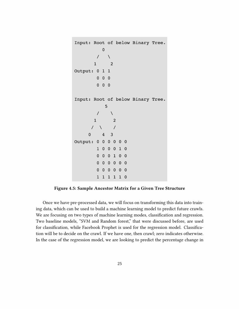
Figure 4.5: Sample Ancestor Matrix for a Given Tree Structure
Once we have pre-processed data, we will focus on transforming this data into train-
ing data, which can be used to build a machine learning model to predict future crawls.
We are focusing on two types of machine learning modes, classi�cation and regression.
Two baseline models, “SVM and Random forest,” that were discussed before, are used
for classi�cation, while Facebook Prophet is used for the regression model. Classi�ca-
tion will be to decide on the crawl. If we have one, then crawl; zero indicates otherwise.
In the case of the regression model, we are looking to predict the percentage change in
25
nodes of a sitemap. If the expected change is above the threshold, we crawl, otherwise
not.
4.3.5 Visualization
For the bene�t of users and researchers alike, the changing sitemaps of websites will be
visualized in a number of di�erent ways.
One such visualization will be a graphic, showing the tree structure with a slider
on the bottom that will allow users to view the tree at di�erent points in time based
on the timestamps assigned to nodes in the constructed tree, as described above. This
visualization will enable users to see how a site has changed over time. New branches
and nodes could even be highlighted when selecting two di�erent time stamps to see
what has changed between them.
Another visualization which is a bit more complicated than the �rst, but that also
provides information in a more interesting way, is known as a treemap. A treemap is
a collection of nested rectangles, with each rectangle representing a branch of the tree.
Using this data structure, we could adjust the colors of branches to indicate how much
the structure of a branch has changed, enabling users to see what areas of the sitemap
change the most over time. This visualization would require a user to select an interval
of time for the algorithm to compare the tree structures.
4.4 Model Web Page Content Change with Reinforce-ment Deep Learning
In this section, we �rst illustrate the RL model environment. Then, we talk about two
RL agent action strategies for our crawling scheduling problem. Next, we discuss the
learning policy algorithms. Our model is implemented through OpenAI’s Gym [2] and
Stable Baselines [7] libraries.
4.4.1 Environment and Observation Space
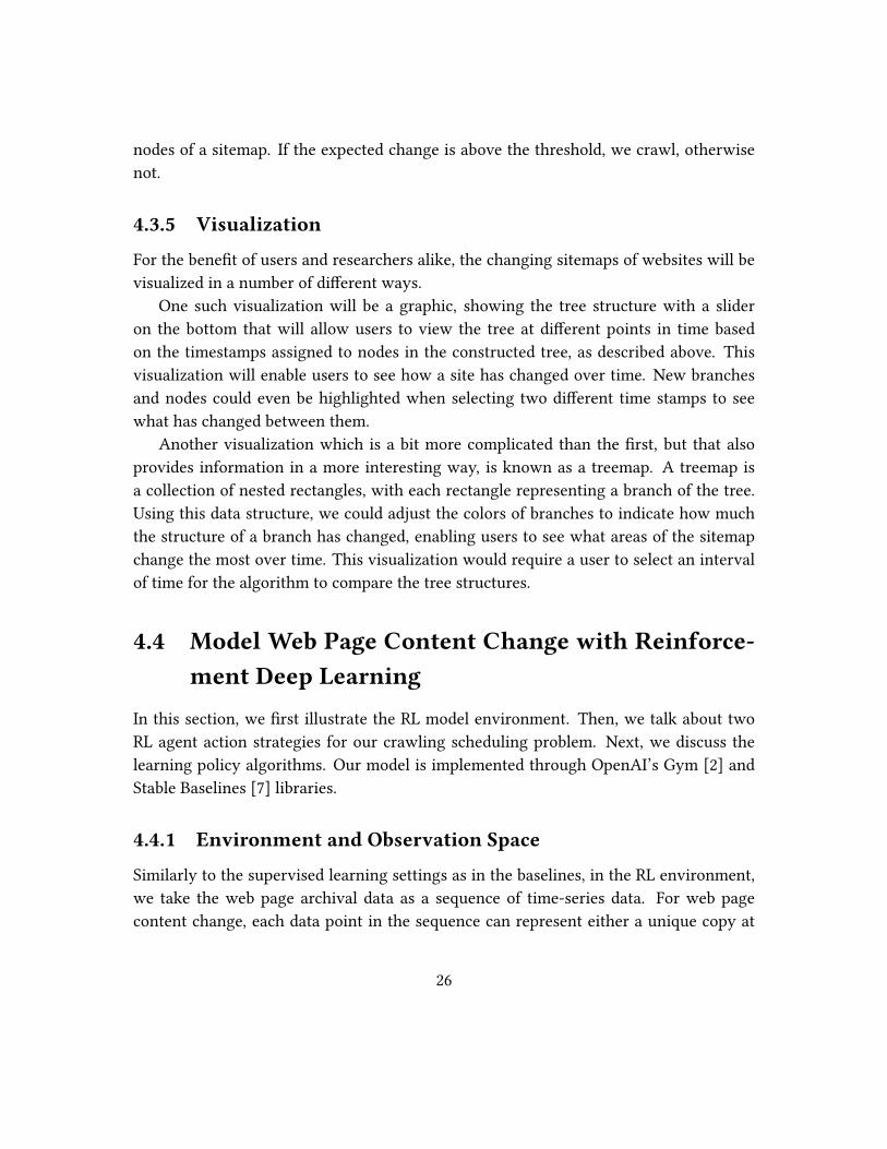
Similarly to the supervised learning settings as in the baselines, in the RL environment,
we take the web page archival data as a sequence of time-series data. For web page
content change, each data point in the sequence can represent either a unique copy at
26
Figure 4.6: A general view of our proposed reinforcement learning environmentfor the web crawling task for one time step: At each time step, the agent willlearn from the historical observation and perform a prede�ned crawling action.Then the slidingwindowwillmove forward andmake a newhistory observationthat includes the previous action.
a certain time or a duplicate copy of a previous unique copy. For web site structure
change, each data point in the sequence represents a unique copy of the current treemap
of the site or a duplicate copy of a previous unique copy. For this project, we primarily
investigate the potential of the RL model to capture the changing behavior of web content
over time. In this case, in the time series data sequence, we mark each earliest data point
with unique information as 1, the other data points with duplicate information as 0.
From the environment, we expect the model to capture the recent changing frequency
of the web page, and then generate a plan to capture the potential future changes ade-
quately. Here, we give a length of Lh hours that the agent can observe in the history
information before each action. By combining the observed history information and im-
mediate action, we can form a sliding window that covers a continuous space within
the data sequence. After each time step, the sliding window will move forward, creating
a new observation space that includes the results from the previous action. Figure 4.6
shows a general view of the process.
4.4.2 Agent, Action, and Reward
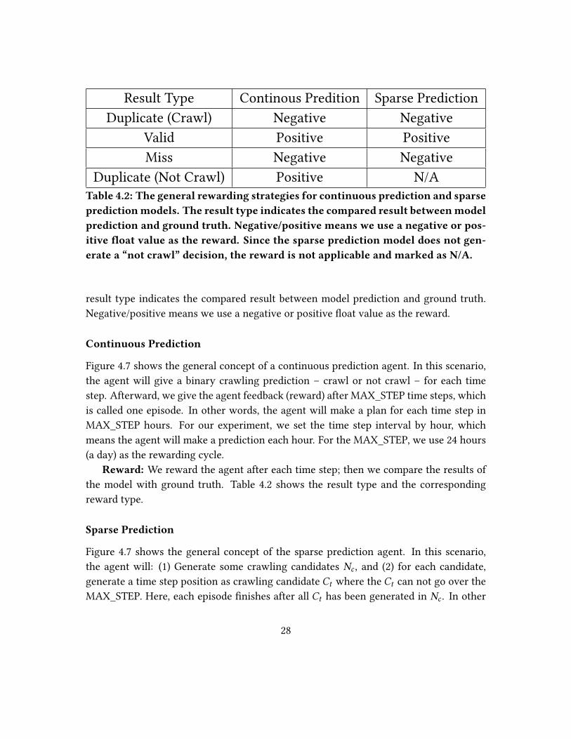
Based on the given environment we de�ned earlier, we can further design the behavior of
the RL agent within the environment and corresponding rewards. We propose two agent
strategies for the crawler: continuous prediction and sparse prediction. In Figure 4.7, the
27
Result Type Continous Predition Sparse Prediction
Duplicate (Crawl) Negative Negative
Valid Positive Positive
Miss Negative Negative
Duplicate (Not Crawl) Positive N/A
Table 4.2: The general rewarding strategies for continuous prediction and sparsepredictionmodels. The result type indicates the compared result betweenmodelprediction and ground truth. Negative/positive means we use a negative or pos-itive �oat value as the reward. Since the sparse prediction model does not gen-erate a “not crawl” decision, the reward is not applicable and marked as N/A.
result type indicates the compared result between model prediction and ground truth.
Negative/positive means we use a negative or positive �oat value as the reward.
Continuous Prediction
Figure 4.7 shows the general concept of a continuous prediction agent. In this scenario,
the agent will give a binary crawling prediction – crawl or not crawl – for each time
step. Afterward, we give the agent feedback (reward) after MAX_STEP time steps, which
is called one episode. In other words, the agent will make a plan for each time step in
MAX_STEP hours. For our experiment, we set the time step interval by hour, which
means the agent will make a prediction each hour. For the MAX_STEP, we use 24 hours
(a day) as the rewarding cycle.
Reward: We reward the agent after each time step; then we compare the results of
the model with ground truth. Table 4.2 shows the result type and the corresponding
reward type.
Sparse Prediction
Figure 4.7 shows the general concept of the sparse prediction agent. In this scenario,
the agent will: (1) Generate some crawling candidates Nc , and (2) for each candidate,
generate a time step position as crawling candidate Ct where the Ct can not go over the
MAX_STEP. Here, each episode �nishes after all Ct has been generated in Nc . In other
28
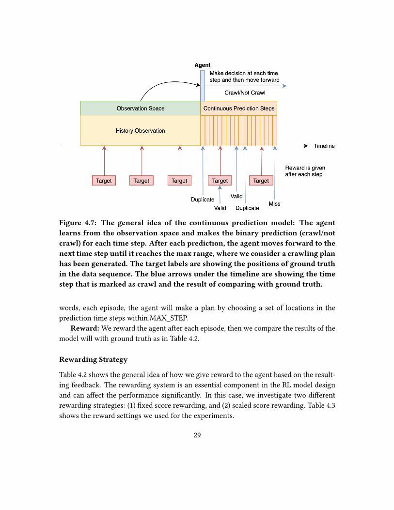
Figure 4.7: The general idea of the continuous prediction model: The agentlearns from the observation space and makes the binary prediction (crawl/notcrawl) for each time step. After each prediction, the agent moves forward to thenext time step until it reaches themax range, where we consider a crawling planhas been generated. The target labels are showing the positions of ground truthin the data sequence. The blue arrows under the timeline are showing the timestep that is marked as crawl and the result of comparing with ground truth.
words, each episode, the agent will make a plan by choosing a set of locations in the
prediction time steps within MAX_STEP.
Reward: We reward the agent after each episode, then we compare the results of the
model will with ground truth as in Table 4.2.
Rewarding Strategy
Table 4.2 shows the general idea of how we give reward to the agent based on the result-
ing feedback. The rewarding system is an essential component in the RL model design
and can a�ect the performance signi�cantly. In this case, we investigate two di�erent
rewarding strategies: (1) �xed score rewarding, and (2) scaled score rewarding. Table 4.3
shows the reward settings we used for the experiments.
29
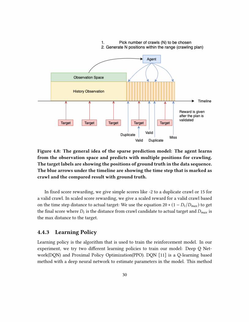
Figure 4.8: The general idea of the sparse prediction model: The agent learnsfrom the observation space and predicts with multiple positions for crawling.The target labels are showing the positions of ground truth in the data sequence.The blue arrows under the timeline are showing the time step that is marked ascrawl and the compared result with ground truth.
In �xed score rewarding, we give simple scores like -2 to a duplicate crawl or 15 for
a valid crawl. In scaled score rewarding, we give a scaled reward for a valid crawl based
on the time step distance to actual target: We use the equation 20 ∗ (1 − Dt/Dmax ) to get
the �nal score where Dt is the distance from crawl candidate to actual target and Dmax is
the max distance to the target.
4.4.3 Learning Policy
Learning policy is the algorithm that is used to train the reinforcement model. In our
experiment, we try two di�erent learning policies to train our model: Deep Q Net-
work(DQN) and Proximal Policy Optimization(PPO). DQN [11] is a Q-learning based
method with a deep neural network to estimate parameters in the model. This method
30
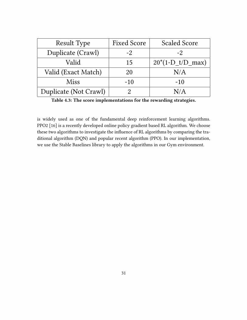
Result Type Fixed Score Scaled Score
Duplicate (Crawl) -2 -2
Valid 15 20*(1-D_t/D_max)
Valid (Exact Match) 20 N/A
Miss -10 -10
Duplicate (Not Crawl) 2 N/A
Table 4.3: The score implementations for the rewarding strategies.
is widely used as one of the fundamental deep reinforcement learning algorithms.
PPO2 [16] is a recently developed online policy gradient based RL algorithm. We choose
these two algorithms to investigate the in�uence of RL algorithms by comparing the tra-
ditional algorithm (DQN) and popular recent algorithm (PPO). In our implementation,
we use the Stable Baselines library to apply the algorithms in our Gym environment.
31
Chapter 5
Evaluation
5.1 Supervised Learning Baselines
Each Machine Learning algorithm has its nuances that capture a particular perspective
of the dataset and the problem statement. The quantitative validation of the results of
an algorithm need to be done to know how well it performs. For the baseline models
discussed earlier, we calculate the Precision, Recall, F1 score, and Accuracy to evaluate
them. In the information retrieval domain, Precision de�nes how many of the extracted
data points are correct, whereas the Recall de�nes what proportion of correct data points
have been extracted from the corpus of all correct. The F1 score is the harmonic mean of
precision and recall.
Precision =True Positives
True Positives + False Postitives
(5.1)
Recall =True Positives
True Positives + False Negatives
(5.2)
F1 − Score =2 · Precision · Recall
Precision + Recall(5.3)
Accuracy =TP +TN
TP +TN + FP + FN(5.4)
where, TP = True Positives, TN = True Negatives, FP = False Positives, and FN = False
Negatives.
32
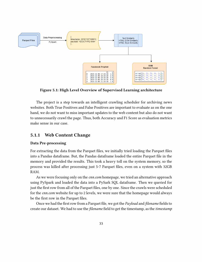
Figure 5.1: High Level Overview of Supervised Learning architecture
The project is a step towards an intelligent crawling scheduler for archiving news
websites. Both True Positives and False Positives are important to evaluate as on the one
hand, we do not want to miss important updates to the web content but also do not want
to unnecessarily crawl the page. Thus, both Accuracy and F1 Score as evaluation metrics
make sense in our case.
5.1.1 Web Content Change
Data Pre-processing
For extracting the data from the Parquet �les, we initially tried loading the Parquet �les
into a Pandas dataframe. But, the Pandas dataframe loaded the entire Parquet �le in the
memory and provided the results. This took a heavy toll on the system memory, so the
process was killed after processing just 5-7 Parquet �les, even on a system with 32GB
RAM.
As we were focusing only on the cnn.com homepage, we tried an alternative approach
using PySpark and loaded the data into a PySark SQL dataframe. Then we queried for
just the �rst row from all of the Parquet �les, one by one. Since the crawls were scheduled
for the cnn.com website for up to 2 levels, we were sure that the homepage would always
be the �rst row in the Parquet �les.
Once we had the �rst row from a Parquet �le, we got the Payload and �lename �elds to
create our dataset. We had to use the �lename �eld to get the timestamp, as the timestamp
33
�eld itself was in YYYYMMDD format. We needed a granularity of up to hours, minutes,
and seconds to get a better idea of the crawl schedules. The �lename �eld contained the
actual time of the crawl up to the second, and so we decided to get the actual timestamp
from the �lename instead. Then we sort the entries based on the timestamp so that we
have the data in chronological order.
After getting the payload and timestamp information for the cnn.com homepage from
all the Parquet �les, we saved the data into a .pkl �le that could be used as needed for
training the di�erent baseline models. In total we had 198 data points ranging from
November 6 to 19, 2019. We used a split of 8:2 for training and testing for the classi�cation
task.
SVM and Random Forests
While using the baseline SVM and Random Forest models, our aim was to be able to
classify whether the web page should be crawled in the next hour or not. From the
stored .pkl �le, we �rst set the �rst entry as the base web page. We then calculate several
metrics for comparing the HTML structure and text content of the subsequent snapshots
to the base web page.
We used BeautifulSoup to extract the visible text content for the web pages. But, the
extracted text mainly contained the header and footer text that did not change much dur-
ing the time period of the dataset. We then realized that this was because the main body
of the web page was being generated by JavaScript and was not captured as part of the
<body> tag in the payload. Upon examining the payload more closely, we found a JSON
object with the key ArticleList that contained a list of headlines and then observed that
the actual headlines displayed on the homepage were actually a subset of the headlines
present in this list. So, we decided to get the ArticleList object from within the <script>
tag from the payload and run our text similarity measures on this list as well.
The calculated metrics are:
• Overall Similarity: Overall structural and style similarity between the current ver-
sion and the last archived snapshot of the web page.
• Style Similarity: The CSS style similarity between the current version and the last
archived snapshot of the web page.
• Structural Similarity: The HTML tree similarity between the current version and
the last archived snapshot of the web page.
34
• Cosine Similarity: The cosine similarity measure between the text extracted by
BeautifulSoup for the current version and the last archived snapshot of the web
page.
• Jaccard Similarity: The jaccard similarity measure between the text extracted by
BeautifulSoup for the current version and the last archived snapshot of the web
page.
• Sorensen Dice Similarity: The sorensen dice similarity measure between the text
extracted by BeautifulSoup for the current version and the last archived snapshot
of the web page.
• Cosine Similarity Article List: The cosine similarity measure between the Arti-cleList for the current version and the last archived snapshot of the web page.
• Jaccard Similarity Article List: The jaccard similarity measure between the Arti-cleList for the current version and the last archived snapshot of the web page.
• Sorensen Dice Similarity Article List: The sorensen dice similarity measure be-
tween the ArticleList for the current version and the last archived snapshot of the
web page.
After calculating and studying these similarity values, we decided to set the thresh-
olds for considering the web page as changed as 0.98 for the overall structural and style
similarity, 1 for the cosine similarity for the text extracted by BeautifulSoup, and 0.97 for
the cosine similarity of the ArticleList. If any of these values was below the respective
thresholds, we set the label for that particular record as 1, signifying a signi�cant change
in the web page and set the current snapshot as the new base snapshot.
We used scikit-learn’s SVM and Random Forest classi�ers to train and test our mod-
els. To train our SVM and Random Forest classi�er with the time series data, we used
windows of multiple hours. Within the speci�ed window, we used the time di�erence
from the last archived web page as the training data along with the label of the imme-
diate next snapshot as the label for the time window. The classi�ers were restricted to
have just 2-dimensional data as training input, so we could not use all of the measures
for each record in the windows as that made the training data 3-dimensional. So, we just
kept windows of time di�erences from the last archived snapshot as the training data as
we felt that it would best capture the time between the changes on the web page. Upon
performing several experiments, we settled on a window size of 5 hours.
35
Model Accuracy Precision Recall F1 Score
Support Vector Machine 0.769 0.74 0.77 0.75
Random Forest 0.615 0.60 0.62 0.61
Table 5.1: Model Evaluation
Facebook Prophet
Prophet restricts the input for the model to be just timestamps and the corresponding
labels. Hence we decided that having the time di�erence from the last archived snapshot
would be a viable continuous label for the dataset, which would become 0 if the current
page was considered to be changed.
The steps to create the training data for Prophet were similar to what was described in
the previous section. The process to determine whether the current snapshot is di�erent
from the last archived snapshot is exactly the same. Once the similarity is determined,
the timestamp and the time di�erence in hours is added to the training data. The time
di�erence is set to 0 in case the web page is considered to be changed, as this value will
be considered the label by Prophet, and setting all changed web pages to have label 0
distinguishes them from the unchanged web pages.
Once we have the timestamps and the time di�erences for all snapshots, we train the
Facebook Prophet model.
Evaluations
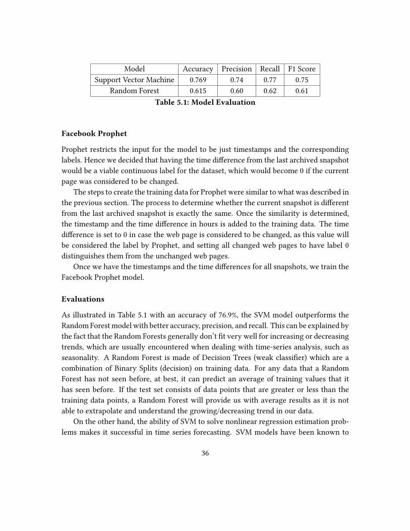
As illustrated in Table 5.1 with an accuracy of 76.9%, the SVM model outperforms the
Random Forest model with better accuracy, precision, and recall. This can be explained by
the fact that the Random Forests generally don’t �t very well for increasing or decreasing
trends, which are usually encountered when dealing with time-series analysis, such as
seasonality. A Random Forest is made of Decision Trees (weak classi�er) which are a
combination of Binary Splits (decision) on training data. For any data that a Random
Forest has not seen before, at best, it can predict an average of training values that it
has seen before. If the test set consists of data points that are greater or less than the
training data points, a Random Forest will provide us with average results as it is not
able to extrapolate and understand the growing/decreasing trend in our data.
On the other hand, the ability of SVM to solve nonlinear regression estimation prob-
lems makes it successful in time series forecasting. SVM models have been known to
36
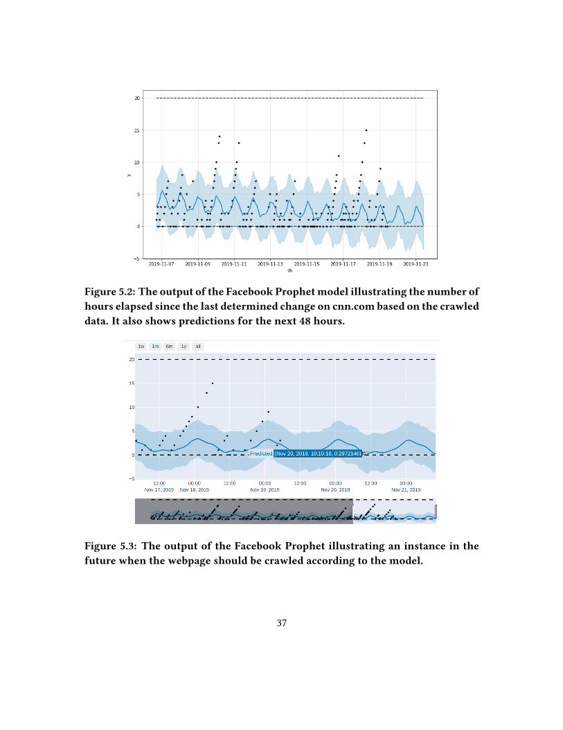
Figure 5.2: The output of the Facebook Prophetmodel illustrating the number ofhours elapsed since the last determined change on cnn.com based on the crawleddata. It also shows predictions for the next 48 hours.
Figure 5.3: The output of the Facebook Prophet illustrating an instance in thefuture when the webpage should be crawled according to the model.
37
handle higher dimensional data better, even with a relatively low amount of training
samples. They exhibit a very good generalization ability for complex models.
Facebook Prophet has an inbuilt feature that enabled us to plot the forecasts it gen-
erated. In Figures 5.2 and 5.3, the blue line in the graph represents the predicted values
while the black dots represent the data in our dataset. We also show the future predic-
tions for the next 48 hours in the graphs. Prophet successfully captures the trend from
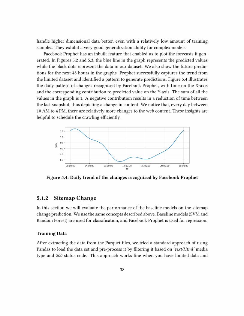
the limited dataset and identi�ed a pattern to generate predictions. Figure 5.4 illustrates
the daily pattern of changes recognised by Facebook Prophet, with time on the X-axis
and the corresponding contribution to predicted value on the Y-axis. The sum of all the
values in the graph is 1. A negative contribution results in a reduction of time between
the last snapshot, thus depicting a change in content. We notice that, every day between
10 AM to 4 PM, there are relatively more changes to the web content. These insights are
helpful to schedule the crawling e�ciently.
Figure 5.4: Daily trend of the changes recognised by Facebook Prophet
5.1.2 Sitemap Change
In this section we will evaluate the performance of the baseline models on the sitemap
change prediction. We use the same concepts described above. Baseline models (SVM and
Random Forest) are used for classi�cation, and Facebook Prophet is used for regression.
Training Data
After extracting the data from the Parquet �les, we tried a standard approach of using
Pandas to load the data set and pre-process it by �ltering it based on ‘text/Html’ media
type and 200 status code. This approach works �ne when you have limited data and
38
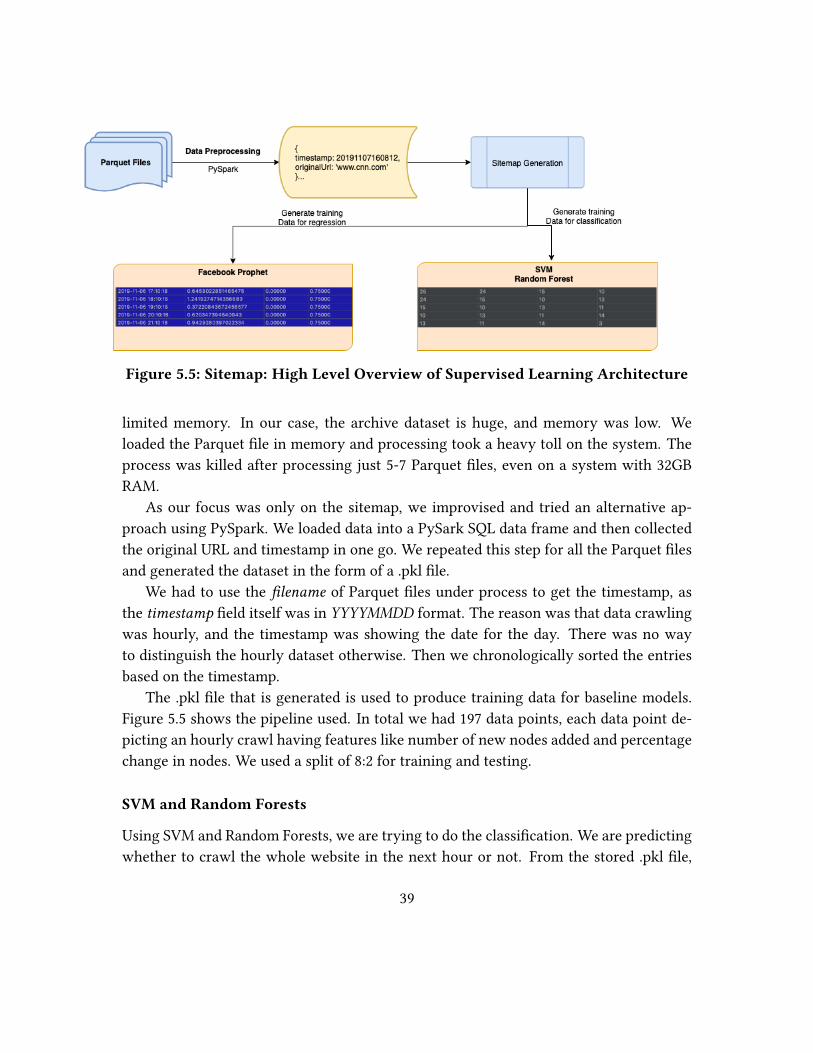
Figure 5.5: Sitemap: High Level Overview of Supervised Learning Architecture
limited memory. In our case, the archive dataset is huge, and memory was low. We
loaded the Parquet �le in memory and processing took a heavy toll on the system. The
process was killed after processing just 5-7 Parquet �les, even on a system with 32GB
RAM.
As our focus was only on the sitemap, we improvised and tried an alternative ap-
proach using PySpark. We loaded data into a PySark SQL data frame and then collected
the original URL and timestamp in one go. We repeated this step for all the Parquet �les
and generated the dataset in the form of a .pkl �le.
We had to use the �lename of Parquet �les under process to get the timestamp, as
the timestamp �eld itself was in YYYYMMDD format. The reason was that data crawling
was hourly, and the timestamp was showing the date for the day. There was no way
to distinguish the hourly dataset otherwise. Then we chronologically sorted the entries
based on the timestamp.
The .pkl �le that is generated is used to produce training data for baseline models.
Figure 5.5 shows the pipeline used. In total we had 197 data points, each data point de-
picting an hourly crawl having features like number of new nodes added and percentage
change in nodes. We used a split of 8:2 for training and testing.
SVM and Random Forests
Using SVM and Random Forests, we are trying to do the classi�cation. We are predicting
whether to crawl the whole website in the next hour or not. From the stored .pkl �le,
39
we will build the site map. As we will make the sitemap, we will also save the new
nodes added in each crawl as a feature. Another feature that we added is the percentage
change from the last checkpoint. A checkpoint is de�ned as the time when the new nodes
added causes the change to pass a set threshold set, e.g., 0.75. It signi�es the percentage
change. If 0.75 percent of nodes were added, then the whole website should be crawled.
I arrived at 0.75 after looking at the general pattern of the nodes added and predicting
the best percentage change that will work. To build the dataset for classi�cation, we
use a time window of 5 hours. Each hour will represent the new nodes added at the
hour for the corresponding crawl. We will use the past �ve values to predict the current.
The corresponding label will be de�ned as zero or one based on the percentage change
since the last checkpoint. The checkpoint is represented as the point when the number
of nodes added passes the threshold. We follow a cumulative type of strategy. For the
current node, if new nodes added since the last checkpoint is higher than the threshold, it
will become new checkpoint and labeled as one, i.e., to crawl otherwise it will be marked
as zero, i.e., not to crawl and its nodes will be added to next and checked again for that
node. It will help the model to learn when to crawl the website i.e., when there is a
signi�cant change in the site structure. Please see Figure 5.5. The generating training
data for classi�cation step is showing the same thing, and the picture shows the �nal
matrix created.
Facebook Prophet
As discussed in previous sections, the Prophet restricts the input for the model to just
timestamps and the corresponding label. In our case, we tried to predict the percentage
change. An hourly crawl timestamp will represent the Prophet’s timestamp requirement.
The corresponding label is the percentage change in nodes since the last checkpoint.
Once we have the dataset created, we train the Facebook Prophet model.
Evaluations
Table 5.2 shows the evaluation results for the predictions by SVM and Random Forest.
Among baseline models, SVM showed an accuracy of 71%. It does perform better as com-
pared to the Random Forest model, with better accuracy and recall, but lower precision.
A possible reason is that Random Forests generally don’t �t very well for increasing or
decreasing trends, especially when dealing with time-series analysis. In contrast, the
40
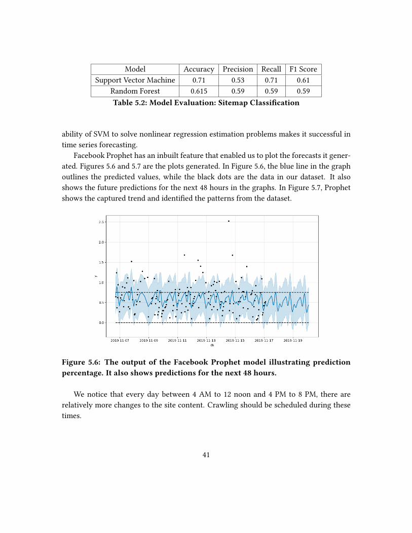
Model Accuracy Precision Recall F1 Score
Support Vector Machine 0.71 0.53 0.71 0.61
Random Forest 0.615 0.59 0.59 0.59
Table 5.2: Model Evaluation: Sitemap Classi�cation
ability of SVM to solve nonlinear regression estimation problems makes it successful in
time series forecasting.
Facebook Prophet has an inbuilt feature that enabled us to plot the forecasts it gener-
ated. Figures 5.6 and 5.7 are the plots generated. In Figure 5.6, the blue line in the graph
outlines the predicted values, while the black dots are the data in our dataset. It also
shows the future predictions for the next 48 hours in the graphs. In Figure 5.7, Prophet
shows the captured trend and identi�ed the patterns from the dataset.
Figure 5.6: The output of the Facebook Prophet model illustrating predictionpercentage. It also shows predictions for the next 48 hours.
We notice that every day between 4 AM to 12 noon and 4 PM to 8 PM, there are
relatively more changes to the site content. Crawling should be scheduled during these
times.
41
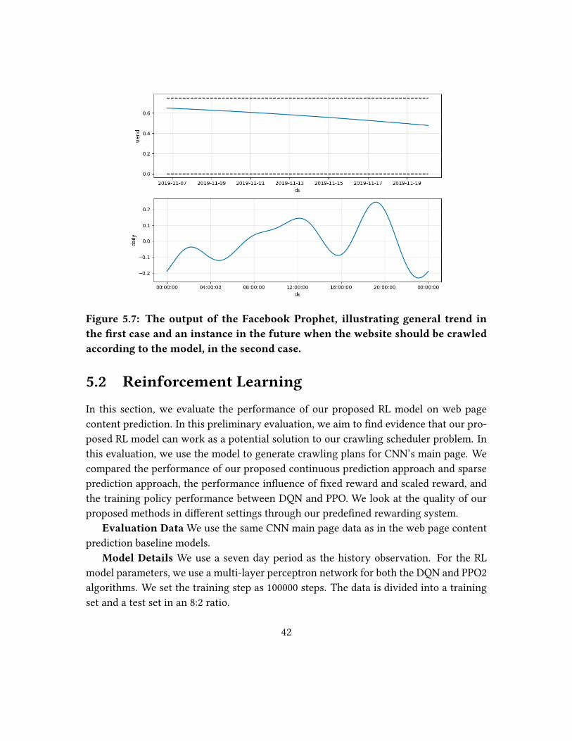
Figure 5.7: The output of the Facebook Prophet, illustrating general trend inthe �rst case and an instance in the future when the website should be crawledaccording to the model, in the second case.
5.2 Reinforcement Learning
In this section, we evaluate the performance of our proposed RL model on web page
content prediction. In this preliminary evaluation, we aim to �nd evidence that our pro-
posed RL model can work as a potential solution to our crawling scheduler problem. In
this evaluation, we use the model to generate crawling plans for CNN’s main page. We
compared the performance of our proposed continuous prediction approach and sparse
prediction approach, the performance in�uence of �xed reward and scaled reward, and
the training policy performance between DQN and PPO. We look at the quality of our
proposed methods in di�erent settings through our prede�ned rewarding system.
Evaluation Data We use the same CNN main page data as in the web page content
prediction baseline models.
Model Details We use a seven day period as the history observation. For the RL
model parameters, we use a multi-layer perceptron network for both the DQN and PPO2
algorithms. We set the training step as 100000 steps. The data is divided into a training
set and a test set in an 8:2 ratio.
42
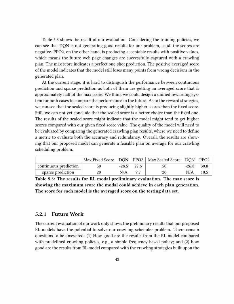
Table 5.3 shows the result of our evaluation. Considering the training policies, we
can see that DQN is not generating good results for our problem, as all the scores are
negative. PPO2, on the other hand, is producing acceptable results with positive values,
which means the future web page changes are successfully captured with a crawling
plan. The max score indicates a perfect one-shot prediction. The positive averaged score
of the model indicates that the model still loses many points from wrong decisions in the
generated plan.
At the current stage, it is hard to distinguish the performance between continuous
prediction and sparse prediction as both of them are getting an averaged score that is
approximately half of the max score. We think we could design a uni�ed rewarding sys-
tem for both cases to compare the performance in the future. As to the reward strategies,
we can see that the scaled score is producing slightly higher scores than the �xed score.
Still, we can not yet conclude that the scaled score is a better choice than the �xed one.
The results of the scaled score might indicate that the model might tend to get higher
scores compared with our given �xed score value. The quality of the model will need to
be evaluated by comparing the generated crawling plan results, where we need to de�ne
a metric to evaluate both the accuracy and redundancy. Overall, the results are show-
ing that our proposed model can generate a feasible plan on average for our crawling
scheduling problem.
Max Fixed Score DQN PPO2 Max Scaled Score DQN PPO2
continuous prediction 50 -28.5 27.6 50 -26.8 30.8
sparse prediction 20 N/A 9.7 20 N/A 10.5
Table 5.3: The results for RL modal preliminary evaluation. The max score isshowing the maximum score the modal could achieve in each plan generation.The score for each model is the averaged score on the testing data set.
5.2.1 Future Work
The current evaluation of our work only shows the preliminary results that our proposed
RL models have the potential to solve our crawling scheduler problem. There remain
questions to be answered: (1) How good are the results from the RL model compared
with prede�ned crawling policies, e.g., a simple frequency-based policy; and (2) how
good are the results from RL model compared with the crawling strategies built upon the
43
supervised machine learning models as in baselines. For future work, we need to build
a uni�ed standard to compare the performance of these di�erent methods so that the
performance of di�erent models can be evaluated quantitatively. We also need a uni�ed
rewarding architecture where we can measure the di�erent RL action models. On top of
the prediction models we have covered in baselines, we need to build a corresponding
crawling plan generation system that can produce the scheduler results.
5.3 Conclusion
In this chapter, we have implemented several traditional supervised machine learning
models on the problem of predicting web content changes. We have also explored re-
inforcement learning models that can generate web crawling plans. The preliminary
result shows that the RL model has the potential to work as an intelligent web crawling
scheduler. We will cover the future works in Chapter 7 regarding further plans for this
research.
44

Chapter 6
Future Work
6.1 Evaluation
We have mentioned the inadequacies of our model evaluation. In future work, we will
need to implement an evaluation method that can evaluate di�erent methods for the
crawling scheduler problem fairly. Currently, we propose to use the generated crawling
plans as the �nal results for comparison. We will need to de�ne a set of metrics for
evaluating the crawling plan results: the freshness of the capture, accuracy of the model,
and resource consumption.
6.2 Further Baseline Model Design
The current baselines we have included in the project can only make predictions for
web content changes. In the future, we need to design the model to generate the actual
crawling plans. What is more, we have only covered the simple models in our literature
review. We should implement or reproduce some more recent works such as [10, 13].
6.3 Further RL Model Design
For further RL model design, we will work on the following improvements:
• Tune the model for optimal performance regarding the web page crawling schedul-
ing problem in this project
45

• Apply the model for web site structure change to see if transfer learning is possible
• Design an RL model that can combine the web page crawling plan and web site
crawling plan
• Explore more features that might bene�t the model on top of the web content
changing frequencies
46
Chapter 7
Lessons Learned
7.1 Data Pre-processing
While developing the project we faced some challenges due to the size of the data and
complexity of the tasks involved.
For the supervised learning task to predict web page changes, we used 14 days of data
corresponding to cnn.com. Although we would get some trends from this limited data,
a larger time series dataset spanning multiple web pages is needed to properly evaluate
the model and recognize the trends. But in the case of sitemap change, we require all the
original webpages crawled during these 14 days since the idea is to catch the trend of the
sitemap change during these hourly crawls.
We initially tried loading the Parquet �les into a Pandas dataframe before extracting
the information from them. Each Parquet �le had roughly 4000 payloads. When trying
to load each one sequentially using Pandas, the system continuously ran out of memory.
We �xed this by using the PySpark SQL dataframe instead, that just loaded the dataframe
schema in memory and collected the results in memory based on the queries made. This
was much more memory e�cient as it did not load each Parquet �le in memory com-
pletely. In case of sitemap predictions, saving the payload while building the sitemap
was appearing to be an onerous task considering the payloads required a lot of space
in memory. We decided to build a sitemap without saving the payload since it is not a
feature in sitemap prediction, thereby decreasing the complexity of building sitemap and
its features for prediction.
47
The timestamps in the Parquet �les were in the YYYYMMDD format, but to properly
capture the trends in the data we required timestamps up to the second. We extracted the
timestamp values for each snapshot based on values from multiple columns in the Parquet
�les. Ideally, there should be a standardized format for storing the timestamp values in
the Parquet �les such that all the necessary information pertaining to the timestamp is
available in a single column.
7.2 Constructing Baselines
To generate the dataset for the supervised learning task for predicting web page changes,
we used thresholds based on cosine and overall HTML structure similarities. The values
of these thresholds were decided by us based on web page di�erences exhibited on the
cnn.com dataset. Ideally, we should conduct human evaluations to prepare ground truth
data and evaluate the threshold values from this data.
The cnn.com web page payload comprises of only the static skeleton of the homepage.
The articles on the page are loaded dynamically using JavaScript. To properly label the
dataset, we extracted this list of articles from the <script> tag and used it in our feature
modelling. Although this is useful to model the data on cnn.com, this is a not a generalised
technique to extract web page content on the internet.
7.3 RL model design
When designing the RL model, all the essential elements – environment, agent, action,
and reward – could make vast di�erences with small changes. We should organize the
code to be prepared for various changes and version tracks. The code should also be
written in a good object-oriented manner. In this way, the model logic will be clearer to
understand and easier to modify. In our current stage, there remain many parts in the
model that need to be tested and validated carefully.
Training a deep RL model can take a very long time, depending on the training steps.
It is useful to use tools such as the Tensor Board to track the training execution. In many
cases, we would get an intuition about the training result from the early stages of training.
Figure 7.1 shows an example of two training processes when we design our model. The
red line is not working well with the training steps, and we should not waste more time
48
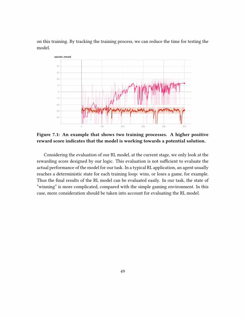
on this training. By tracking the training process, we can reduce the time for testing the
model.
Figure 7.1: An example that shows two training processes. A higher positivereward score indicates that the model is working towards a potential solution.
Considering the evaluation of our RL model, at the current stage, we only look at the
rewarding score designed by our logic. This evaluation is not su�cient to evaluate the
actual performance of the model for our task. In a typical RL application, an agent usually
reaches a deterministic state for each training loop: wins, or loses a game, for example.
Thus the �nal results of the RL model can be evaluated easily. In our task, the state of
“winning” is more complicated, compared with the simple gaming environment. In this
case, more consideration should be taken into account for evaluating the RL model.
49

Chapter 8
Acknowledgements
This project was completed during the course of CS6604 Digital Libraries, at Virginia
Tech. Part of the web archive data was provided by the Internet Archive. Support for
web archiving work at Virginia Tech and Internet Archives was provided by NSF grants
IIS-1619028 and 1619371.
The authors would like to thank Dr. Edward A. Fox and our classmates for providing
insight and expertise that greatly helped us accomplish this research project.
We thank Internet Archive and Mark Graham for providing the web archive data,
insights, and help for the project.
Last but not least, we are immensely grateful to the creators of all the open source
software we used to create this project. Thank you very much!
50

Chapter 9
User Manual
9.1 ArchiveOrgCollectionScraper
Gitlab repo:
https://git.cs.vt.edu/xw0078/archiveorgcollectionscraper
ArchiveOrgCollectionScraper is a web scraper that can fetch all the downloadable
links of collection data from the collection page. An example of usage can be found in
the “GetArchiveOrgDownloadLinks.ipynb” Jupyter Notebook. The code takes the URL of
the target collection. Then it will generate a text �le that contains all the downloadable
links to WARC and CDX �les in the collection. The collection can be downloaded through
Wget:
wget -i urls.txt
Note: You need to have proper user authentication to get access to non-public collec-
tions.
9.2 Zeppelin
O�cial website:
https://zeppelin.apache.org/
Zeppelin is a notebook environment (similar to Jupyter Notebook) that supports mul-
tiple languages and frameworks. In this project, we primarily take advantage of the
Spark integration and Scala programming language. We use Zeppelin to work with the
Web2Warc library and Archive Unleashed Toolkit.
51
9.3 Web2Warc
Github repo:
https://github.com/helgeho/Web2Warc
Web2Warc is a simple and easy crawler that can produce WARC/CDX output. We
modi�ed Web2Warc to collect data that are compatible with AUT. We run Web2Warc
under the Zeppelin environment. Please check the example code under ExampleNote-
books in our project repo: https://git.cs.vt.edu/xw0078/cs-6604-webarchive
9.4 Archive Unleashed Toolkit (AUT)
Github repo:
https://github.com/archivesunleashed/aut/
AUT is a web archive big data processing tool under the Spark environment. We
modi�ed AUT to support extracting more index information as we need it. We run AUT
data conversion under the Zeppelin environment. Please check the example code under
ExampleNotebooks in our project repo: https://git.cs.vt.edu/xw0078/cs-6604-webarchive
9.5 Heritrix
Github repo:
https://github.com/internetarchive/heritrix3
Heritrix is an open source web crawler that is designed by the Internet Archive. A
core concept about Heritrix is that it is designed to work with the "robots.txt" exclusion
directives and META robots tags. In other words, the crawling jobs fully respect the rules
that are de�ned by the web sites creator.
9.6 HTML-Similarity
Github repo:
https://github.com/matiskay/html-similarity
This package provides a set of functions to measure the similarity between web pages.
All the similarity metrics take values between 0 and 1.
52
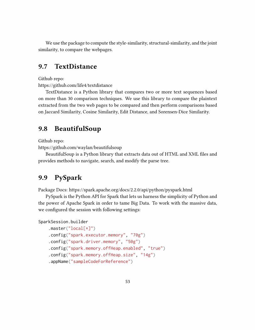
We use the package to compute the style-similarity, structural-similarity, and the joint
similarity, to compare the webpages.
9.7 TextDistance
Github repo:
https://github.com/life4/textdistance
TextDistance is a Python library that compares two or more text sequences based
on more than 30 comparison techniques. We use this library to compare the plaintext
extracted from the two web pages to be compared and then perform comparisons based
on Jaccard Similarity, Cosine Similarity, Edit Distance, and Sorensen-Dice Similarity.
9.8 BeautifulSoup
Github repo:
https://github.com/waylan/beautifulsoup
BeautifulSoup is a Python library that extracts data out of HTML and XML �les and
provides methods to navigate, search, and modify the parse tree.
9.9 PySpark
Package Docs: https://spark.apache.org/docs/2.2.0/api/python/pyspark.html
PySpark is the Python API for Spark that lets us harness the simplicity of Python and
the power of Apache Spark in order to tame Big Data. To work with the massive data,
we con�gured the session with following settings:
SparkSession.builder
.master("local[*]")
.config("spark.executor.memory", "70g")
.config("spark.driver.memory", "50g")
.config("spark.memory.offHeap.enabled", "true")
.config("spark.memory.offHeap.size", "14g")
.appName("sampleCodeForReference")
53
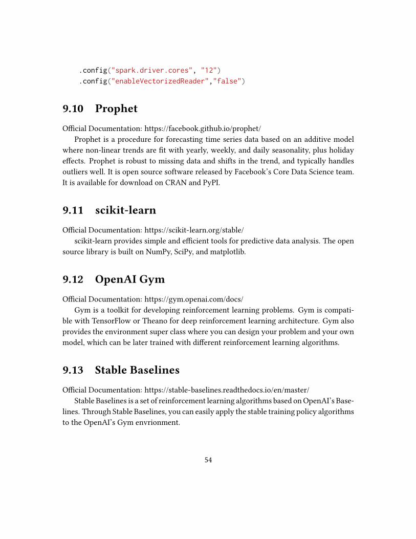
.config("spark.driver.cores", "12")
.config("enableVectorizedReader","false")
9.10 Prophet
O�cial Documentation: https://facebook.github.io/prophet/
Prophet is a procedure for forecasting time series data based on an additive model
where non-linear trends are �t with yearly, weekly, and daily seasonality, plus holiday
e�ects. Prophet is robust to missing data and shifts in the trend, and typically handles
outliers well. It is open source software released by Facebook’s Core Data Science team.
It is available for download on CRAN and PyPI.
9.11 scikit-learn
O�cial Documentation: https://scikit-learn.org/stable/
scikit-learn provides simple and e�cient tools for predictive data analysis. The open
source library is built on NumPy, SciPy, and matplotlib.
9.12 OpenAI Gym
O�cial Documentation: https://gym.openai.com/docs/
Gym is a toolkit for developing reinforcement learning problems. Gym is compati-
ble with TensorFlow or Theano for deep reinforcement learning architecture. Gym also
provides the environment super class where you can design your problem and your own
model, which can be later trained with di�erent reinforcement learning algorithms.
9.13 Stable Baselines
O�cial Documentation: https://stable-baselines.readthedocs.io/en/master/
Stable Baselines is a set of reinforcement learning algorithms based on OpenAI’s Base-
lines. Through Stable Baselines, you can easily apply the stable training policy algorithms
to the OpenAI’s Gym envrionment.
54

Chapter 10
Developer’s Manual
10.1 Project Architecture and Inventory
Our source code is hosted in a GitHub repository at https://git.cs.vt.edu/xw0078/cs-6604-
webarchive.
10.2 File Inventory
1. dataExtract.ipynb is the container notebook for the script to extract the payload
and timestamp data for the cnn.com homepage from the Parquet �les. The root
directory and the URL for which the data is to be extracted are given as input.
The script outputs the timestamp and payload information for the corresponding
URL from all Parquet �les found in the root directory by recursively traversing all
folders. The result is then stored into a .pkl �le archiveData.pkl
2. classifyArchives.ipynb is the container notebook for training the supervised learn-
ing models and making predictions. The archiveData.pkl �le generated by the pre-
vious script is provided as input and the results are the predictions made by the
di�erent supervised learning models along with the evaluations of the predictions.
3. Parquet�leProcessor.ipynb is a container notebook for the script to extract the
timestamp and URL data for hourly crawls from the Parquet �les.
4. Trie.py is a site map creating package.
55
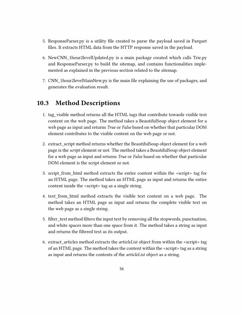
5. ResponseParser.py is a utility �le created to parse the payload saved in Parquet
�les. It extracts HTML data from the HTTP response saved in the payload.
6. NewCNN_1hour2levelUpdated.py is a main package created which calls Trie.py
and ResponseParser.py to build the sitemap, and contains functionalities imple-
mented as explained in the previous section related to the sitemap.
7. CNN_1hour2levelMainNew.py is the main �le explaining the use of packages, and
generates the evaluation result.
10.3 Method Descriptions
1. tag_visible method returns all the HTML tags that contribute towards visible text
content on the web page. The method takes a BeautifulSoup object element for a
web page as input and returns True or False based on whether that particular DOM
element contributes to the visible content on the web page or not.
2. extract_script method returns whether the BeautifulSoup object element for a web
page is the script element or not. The method takes a BeautifulSoup object element
for a web page as input and returns True or False based on whether that particular
DOM element is the script element or not.
3. script_from_html method extracts the entire content within the <script> tag for
an HTML page. The method takes an HTML page as input and returns the entire
content inside the <script> tag as a single string.
4. text_from_html method extracts the visible text content on a web page. The
method takes an HTML page as input and returns the complete visible text on
the web page as a single string.
5. �lter_text method �lters the input text by removing all the stopwords, punctuation,
and white spaces more than one space from it. The method takes a string as input
and returns the �ltered text as its output.
6. extract_articles method extracts the articleList object from within the <script> tag
of an HTML page. The method takes the content within the <script> tag as a string
as input and returns the contents of the articleList object as a string.
56
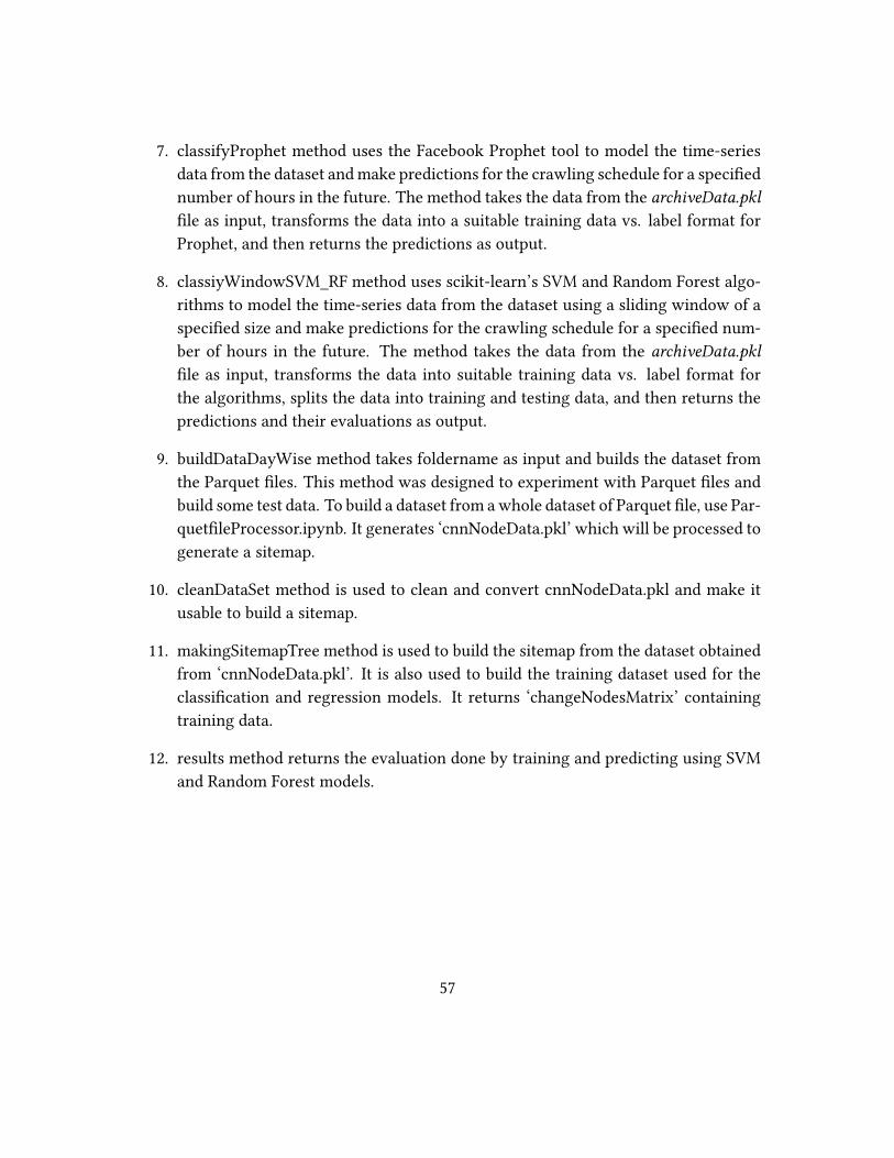
7. classifyProphet method uses the Facebook Prophet tool to model the time-series
data from the dataset and make predictions for the crawling schedule for a speci�ed
number of hours in the future. The method takes the data from the archiveData.pkl�le as input, transforms the data into a suitable training data vs. label format for
Prophet, and then returns the predictions as output.
8. classiyWindowSVM_RF method uses scikit-learn’s SVM and Random Forest algo-
rithms to model the time-series data from the dataset using a sliding window of a
speci�ed size and make predictions for the crawling schedule for a speci�ed num-
ber of hours in the future. The method takes the data from the archiveData.pkl�le as input, transforms the data into suitable training data vs. label format for
the algorithms, splits the data into training and testing data, and then returns the
predictions and their evaluations as output.
9. buildDataDayWise method takes foldername as input and builds the dataset from
the Parquet �les. This method was designed to experiment with Parquet �les and
build some test data. To build a dataset from a whole dataset of Parquet �le, use Par-
quet�leProcessor.ipynb. It generates ‘cnnNodeData.pkl’ which will be processed to
generate a sitemap.
10. cleanDataSet method is used to clean and convert cnnNodeData.pkl and make it
usable to build a sitemap.
11. makingSitemapTree method is used to build the sitemap from the dataset obtained
from ‘cnnNodeData.pkl’. It is also used to build the training dataset used for the
classi�cation and regression models. It returns ‘changeNodesMatrix’ containing
training data.
12. results method returns the evaluation done by training and predicting using SVM
and Random Forest models.
57
Bibliography
[1] Agata, T., Miyata, Y., Ishita, E., Ikeuchi, A., and Ueda, S. Life span of web pages:
A survey of 10 million pages collected in 2001. In IEEE/ACM Joint Conference onDigital Libraries (Sep. 2014), pp. 463–464.
[2] Brockman, G., Cheung, V., Pettersson, L., Schneider, J., Schulman, J., Tang, J.,
and Zaremba, W. Openai gym. CoRR abs/1606.01540 (2016).
[3] Cristianini, N., and Shawe-Taylor, J. An Introduction to Support Vector Machinesand Other Kernel-based Learning Methods. Cambridge University Press, 2000.
[4] Gowda, T., and Mattmann, C. A. Clustering web pages based on structure and
style similarity (application paper). In 2016 IEEE 17th International Conference onInformation Reuse and Integration (IRI) (July 2016), pp. 175–180.
[5] Harvey, A. C., and Peters, S. Estimation procedures for structural time series
models. Journal of Forecasting 9, 2 (1990), 89–108.
[6] Hastie, T., and Tibshirani, R. Generalized additive models: Some applications.
Journal of the American Statistical Association 82, 398 (1987), 371–386.
[7] Hill, A., Raffin, A., Ernestus, M., Gleave, A., Kanervisto, A., Traore, R.,
Dhariwal, P., Hesse, C., Klimov, O., Nichol, A., Plappert, M., Radford, A.,
Schulman, J., Sidor, S., and Wu, Y. Stable baselines. https://github.com/hill-
a/stable-baselines, 2018.
[8] Kahle, B. Preserving the internet. Scienti�c American 276, 3 (1997), 82–83.
[9] Law, M. T., Gutierrez, C. S., Thome, N., Gançarski, S., and Cord, M. Structural
and visual similarity learning for web page archiving. In 2012 10th InternationalWorkshop on Content-Based Multimedia Indexing (CBMI) (2012), IEEE, pp. 1–6.
58
[10] Meegahapola, L., Alwis, R., Nimalarathna, E., Mallawaarachchi, V., Mee-
deniya, D., and Jayarathna, S. Detection of change frequency in web pages to
optimize server-based scheduling. In 2017 Seventeenth International Conference onAdvances in ICT for Emerging Regions (ICTer) (Sep. 2017), pp. 1–7.
[11] Mnih, V., Kavukcuoglu, K., Silver, D., Graves, A., Antonoglou, I., Wierstra,
D., and Riedmiller, M. A. Playing atari with deep reinforcement learning. ArXivabs/1312.5602 (2013).
[12] Pehlivan, Z., Ben-Saad, M., and Gançarski, S. Vi-di�: Understanding web pages
changes. In International Conference on Database and Expert Systems Applications(2010), Springer, pp. 1–15.
[13] Radinsky, K., and Bennett, P. N. Predicting Content Change on the Web. In Pro-ceedings of the Sixth ACM International Conference on Web Search and Data Mining(New York, NY, USA, 2013), WSDM ’13, ACM, pp. 415–424.
[14] Saad, M. B., and Gançarski, S. Using visual pages analysis for optimizing web
archiving. In Proceedings of the 2010 EDBT/ICDT Workshops (New York, NY, USA,
2010), EDBT ’10, ACM, pp. 43:1–43:7.
[15] SalahEldeen, H. M., and Nelson, M. L. Losing my revolution: How many re-
sources shared on social media have been lost? In Theory and Practice of DigitalLibraries (Berlin, Heidelberg, 2012), P. Zaphiris, G. Buchanan, E. Rasmussen, and
F. Loizides, Eds., Springer Berlin Heidelberg, pp. 125–137.
[16] Schulman, J., Wolski, F., Dhariwal, P., Radford, A., and Klimov, O. Proximal
policy optimization algorithms. ArXiv abs/1707.06347 (2017).
[17] Taylor, S., and Letham, B. Forecasting at scale. The American Statistician 72 (09
2017).
[18] Yang, D., and Song, J. Web content information extraction approach based on
removing noise and content-features. In 2010 International Conference on Web In-formation Systems and Mining (Oct 2010), vol. 1, pp. 246–249.
[19] Zhang, K., and Shasha, D. Simple fast algorithms for the editing distance between
trees and related problems. SIAM J. Comput. 18 (12 1989), 1245–1262.
59

Appendix A
Project Plan and Calendar
Calendar and Events Plan
Week Tue Thu
1 27-Aug Forming Team
29-Aug Forming Team
2 3-Sep Forming Team
5-Sep Literature Review
3 10-Sep
Approach proposed
Literature Review
12-Sep
Literature Review
Gather data
Learn tools and background knowledge
4 17-Sep
Literature Review
Gather data
Web page similarity test
Site map comparison
19-Sep
Continuous Work
Sample data prepared
5 24-Sep Continuous Work
26-Sep
Continuous Work
Presentation: Xinyue Wang
60
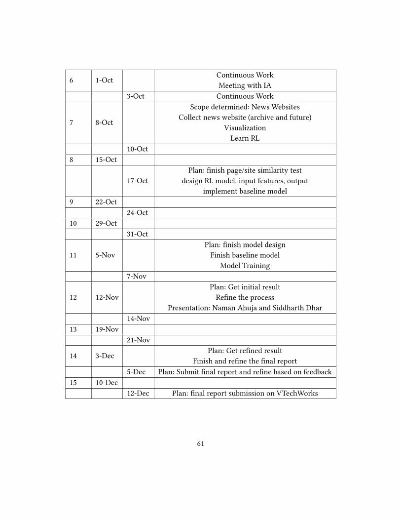
6 1-Oct
Continuous Work
Meeting with IA
3-Oct Continuous Work
7 8-Oct
Scope determined: News Websites
Collect news website (archive and future)
Visualization
Learn RL
10-Oct
8 15-Oct
17-Oct
Plan: �nish page/site similarity test
design RL model, input features, output
implement baseline model
9 22-Oct
24-Oct
10 29-Oct
31-Oct
11 5-Nov
Plan: �nish model design
Finish baseline model
Model Training
7-Nov
12 12-Nov
Plan: Get initial result
Re�ne the process
Presentation: Naman Ahuja and Siddharth Dhar
14-Nov
13 19-Nov
21-Nov
14 3-Dec
Plan: Get re�ned result
Finish and re�ne the �nal report
5-Dec Plan: Submit �nal report and re�ne based on feedback
15 10-Dec
12-Dec Plan: �nal report submission on VTechWorks
61