CS534 Machine Learning

Spring 2012

Course Information

• Instructor: Dr. Xiaoli FernKec 3073, xfern@eecs.oregonstate.edu

• TA: Beatrice Moissinac• Office hour (tentative)

Instructor: MW before class 11‐12 or by appointmentTA: TBA (see class webpage for update)

• Class Web Pageclasses.engr.oregonstate.edu/eecs/spring2012/cs534/

• Class email listcs534‐sp12@engr.orst.edu

Course materials

• Text book (not required), but strongly recommended:– Pattern recognition and machine learning by Chris Bishop (Bishop) 

• Slides and reading materials will be provided on course webpage

• Other good references– Machine learning by Tom Mitchell (TM)– Pattern Classfication by Duda, Hart and Stork (DHS) 2ndedition

• There are a lot of online resources on machine learning– Stanford machine learning lectures by Andrew Ng are available online 

3

Prerequisites

• Multivariable Calculus and linear algebra– Some basic review slides on class webpage– Useful video lectures  ocw.mit.edu/OcwWeb/Mathematics/18‐06Spring‐2005/VideoLectures/index.htmocw.mit.edu/OcwWeb/Mathematics/18‐02Fall 2007/VideoLectures/index.htm

• Basic probability theory and statistics concepts: Distributions, Densities, Expectation, Variance, parameter estimation …

• Knowledge of basic CS concepts such as data structure, search strategies, complexity 

Machine learning

Experience E

Learning Algorithm

Task T Performance P

Machine learning studies algorithms that• Improve performance P• at some task T• based on experience E

Fields of Study

Machine Learning

Supervised Learning

Unsupervised Learning

Reinforcement Learning

Semi‐supervised learning

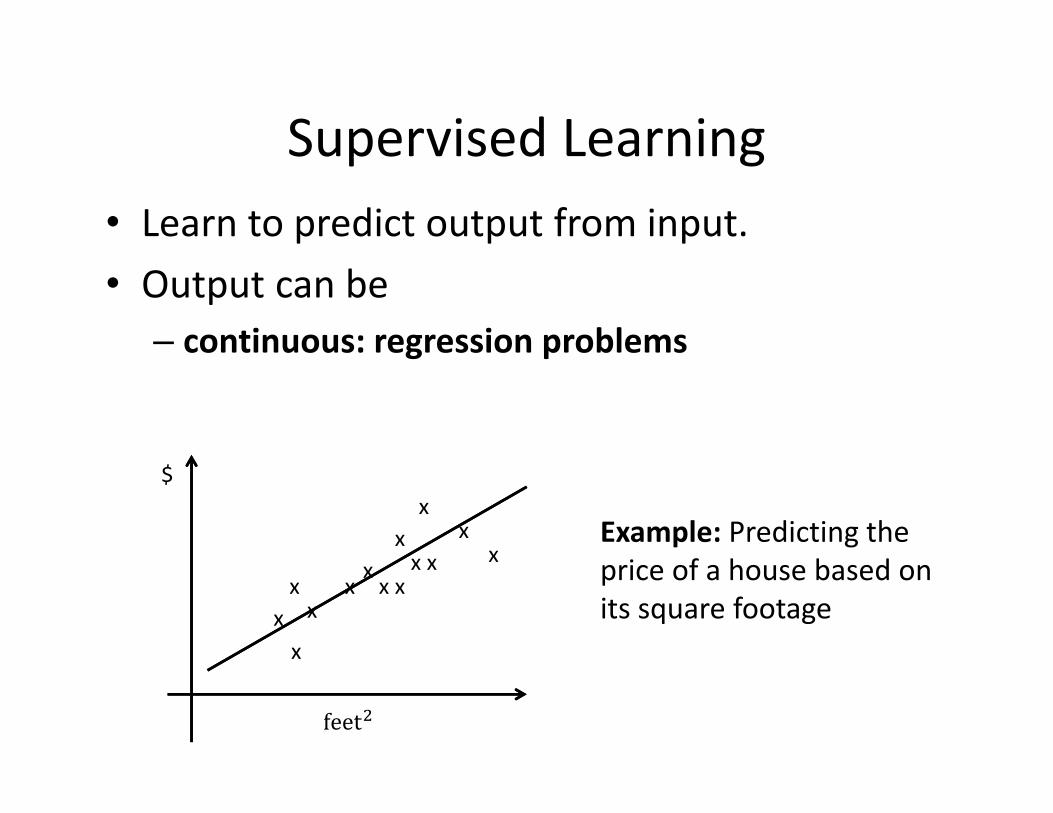
Supervised Learning• Learn to predict output from input. • Output can be 

– continuous: regression problems

Example: Predicting the price of a house based on its square footage

feet

$

xxx

xxx

x

x

x

xxx

x

x

Supervised Learning• Learn to predict output from input. • Output can be 

– continuous: regression problems– Discrete: classification problems

Example: classify a loan applicant as either high risk or low risk based on income and saving amount.

Unsupervised Learning

• Given a collection of examples (objects), discover self‐similar groups within the data –clustering

Example: clustering artwork

11

Unsupervised learning• Given a collection of examples (objects), discover self‐similar groups within the data –clustering

Image Segmentation

Unsupervised Learning

• Given a collection of examples (objects), discover self‐similar groups within the data –clustering

• Learn the underlying distribution that generates the data we observe – density estimation

• Represent high dimensional data using a low‐dimensional representation for compression or visualization – dimension reduction

Reinforcement Learning

• Learn to act• An agent

– Observes the environment– Takes action– With each action, receives rewards/punishments– Goal: learn a policy that optimizes rewards

• No examples of optimal outputs are given• Not covered in this class. Take 533 if you want to learn about this.

When do we need computer to learn?

15

Appropriate Applications for Supervised Learning

• Situations where there is no human expert– x: bond graph of a new molecule– f(x): predicted binding strength to AIDS protease molecule

• Situations where humans can perform the task but can’t describe how they do it– x: picture of a hand‐written character– f(x): ascii code of the character

• Situations where the desired function is changing frequently– x: description of stock prices and trades for last 10 days– f(x): recommended stock transactions

• Situations where each user needs a customized function f– x: incoming email message– f(x): importance score for presenting to the user (or deleting without 

presenting)

Supervised learning

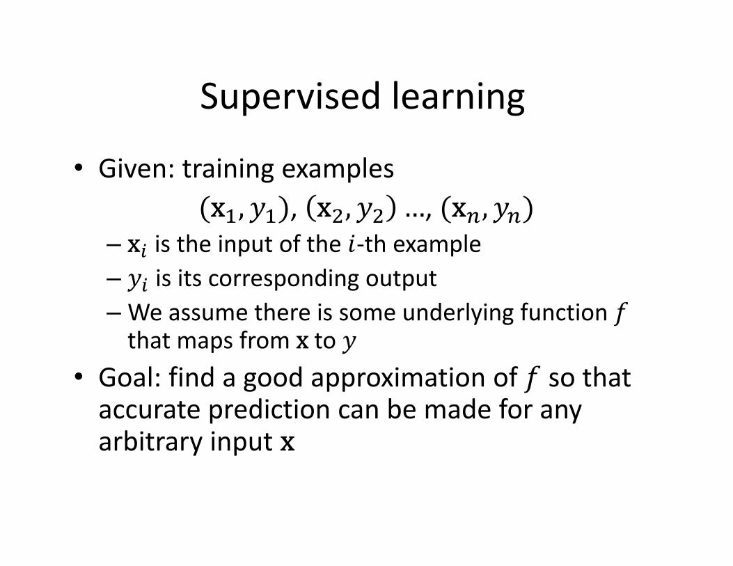
• Given: training examples , ,

– is the input of the  ‐th example– is its corresponding output– We assume there is some underlying function that maps from  to 

• Goal: find a good approximation of  so that accurate prediction can be made for any arbitrary input 

The underline function:

Polynomial curve fitting• There are infinite functions that will fit the training data 

perfectly. In order to learn, we have to focus on a limited set of possible functions – We call this our hypothesis space– E.g., all M‐th order polynomial functions

– w = (w0 , w1 ,…, wM ) represents the unknown parameters that we wish to learn

• Learning  here means  to  find  a  good  set  of  parameters w  to minimize  some  loss  function

MM xwxwxwwxy ...),( 2

210w

This optimization problem can be solved easily.We will not focus on solving this at this point, will revisit this later.

Important Issue: Model Selection

• The red line shows the function learned with different M values• Which M should we choose – this is a model selection problem• Can we use E(w) that we define in previous slides as a criterion to 

choose M?

Over‐fitting• As M increases, training error decreases monotonically

• However, the test error starts to decrease after a while • Why? Is this a fluke or generally true?

It turns out this is generally the case –caused by over‐fitting

Over‐fitting

• Over‐fitting happens when– There is too little data – There are too many the parameters

• Learning algorithm fits to chance statistics• E.g., I am trying to estimate the average snow fall amount of March in Corvallis 

• Using the data from this year, I would conclude that we have a fairly decent amount of snow in Corvallis

• But this estimation will be overfitting to this year’s data 

22

Supervised learning: Formal Setting

• Training examples: drawn independently at random according to unknown distribution P(x,y)

• The learning algorithm analyzes the training examples and produces a classifier f

• Given a new point <x,y> drawn from P,  the classifier is given x and predicts ŷ = f(x)

• The loss L(ŷ,y) is then measured• Goal of the learning algorithm: Find the f that 

minimizes the expected loss , ,

P(x,y) <x,y>

Training sample

learning algorithm f

test point

x

loss function

y

yŷ

training points

L(ŷ,y)

23

Classification Example: Spam Detection• P(x,y): distribution of email messages x and labels y(“spam” or “not spam”)

• Training sample: a set of email messages that have been labeled by the user

• Learning algorithm: what we study in this course!• f: the classifier output by the learning algorithm• Test point: A new email message x (with its true, but hidden, label y)

• loss function L(ŷ,y):

predicted label ŷ

true label yspam None-

spamspam 0 10None-spam

1 0

24

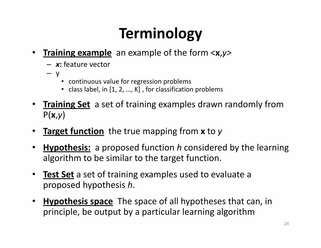
Terminology• Training example an example of the form <x,y>

– x: feature vector– y

• continuous value for regression problems• class label, in [1, 2, …, K] , for classification problems

• Training Set a set of training examples drawn randomly from P(x,y)

• Target function the true mapping from x to y

• Hypothesis: a proposed function h considered by the learning algorithm to be similar to the target function.

• Test Set a set of training examples used to evaluate a proposed hypothesis h. 

• Hypothesis space The space of all hypotheses that can, in principle, be output by a particular learning algorithm

25

Key Issues in Machine Learning• What are good hypothesis spaces?

– Linear functions? Polynomials? – which spaces have been useful in practical applications?

• How to select among different hypothesis spaces?– The Model selection problem– Trade‐off between over‐fitting and under‐fitting

• How can we optimize accuracy on future data points?– This is often called the Generalization Error – error on unseen data pts– Related to the issue of “overfitting”, i.e., the model fitting to the peculiarities 

rather than the generalities of the data  • What level of confidence should we have in the results? (A 

statistical question)– How much training data is required to find an accurate hypotheses with high 

probability?  This is the topic of learning theory• Are some learning problems computationally intractable? (A 

computational question)– Some learning problems are provably hard– Heuristic / greedy approaches are often used when this is the case

• How can we formulate application problems as machine learning problems?  (the engineering question)

Homework Policies

• Homework is due at the beginning of the class on the due day

• Each student has one allowance of handing in late homework (no more than 48 hours late)

• Collaboration policy– Discussions are allowed, but copying of solution or code is not 

– See the Student Conduct page on OSU website for information regarding academic dishonesty (http://oregonstate.edu/studentconduct/code/index.php#acdis)

Grading policy• Grading policy:

Written homework will not be graded based on correctness. We will record the number of problems that were "completed" (either correctly or incorrectly). Completing a problems requires a non‐trivial attempt at solving the problem. The judgment of whether a problem was "completed" is left to the instructor and the TA. 

• Final grades breakdown:– Midterm 25%; Final 25%;  Final project 25%; Implementation 

assignments 25%.– The resulting letter grade will be decreased by one if a student fails 

to complete at least 80% of the written homework problems.