cs5263 bioinformatics
DESCRIPTION
CS5263 Bioinformatics. Lecture 12: Hidden Markov Models and applications. Project ideas. Implement an HMM including Viterbi decoding, posterior decoding and Baum-Welch learning Construct a model Generate sequences with the model Given labels, estimate parameters Given parameters, decode - PowerPoint PPT PresentationTRANSCRIPT

CS5263 Bioinformatics
Lecture 12: Hidden Markov Models and applications

Project ideas
• Implement an HMM including Viterbi decoding, posterior decoding and Baum-Welch learning– Construct a model– Generate sequences with the model– Given labels, estimate parameters– Given parameters, decode– Given nothing, learn the parameters and
decode

Project ideas
• Implement a progressive multiple sequence alignment with iterative refinement– Use an inferred phylo-genetic tree– Affine gap penalty?– Compare with results in protein families?– Compare with HMM-based?

Project ideas
• Implement a combinatorial motif finder– Fast enumeration using suffix tree?– Statistical evaluation– Word clustering?– Test on simulated data – can you find known
motifs embedded in sequences– Test on real data – find motifs in some real
promoter sequences and compare with what is known about those genes

Project ideas
• Pick a paper about some algorithm and implement it
• Do your own experiments
• Or pick a topic and do a survey

Problems in HMM
• Decoding– Predict the state of each symbol
• Most probable path• Most probable state for each position: posterior decoding
• Evaluation– The probability that a sequence is generated by a
model– Basis for posterior decoding
• Learning– Decode without knowing model parameters– Estimate parameters without knowing states
• Review of last lecture

Decoding
Input: HMM & transition and emission parameters, and a sequence
Output: the state of each position on the sequence
?
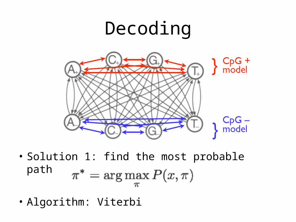
Decoding
• Solution 1: find the most probable path
• Algorithm: Viterbi

HMM for loaded/fair dice
Fair LOADED
aLF = 0.05
eF(1) = 1/6eF(2) = 1/6eF(3) = 1/6eF(4) = 1/6eF(5) = 1/6eF(6) = 1/6
eL(1) = 1/10eL(2) = 1/10eL(3) = 1/10eL(4) = 1/10eL(5) = 1/10eL(6) = 1/2
Probability of a path is the product of transition probabilities and emission probabilities on the path
Transition probability
Emission probability
aFL = 0.05 aLL = 0.95aFF = 0.95

HMM unrolled
x1 x2 x3 x4 x5 x6 x7 x8 x9 x10
F
L
F
L
F
L
F
L
F
L
F
L
F
L
F
L
F
L
F
L
B
Node weight r(F, x) = log (eF(x))Edge weight w(F, L) = log (aFL)
Find a path with the following objective:
• Maximize the product of transition and emission probabilities Maximize the sum of weights
Strategy: Dynamic Programming

FSA interpretation
Fair LOADED
aFL= 0.05
Fair LOADED
w(F,F) = 2.3
r(F,1) = 0.5r(F,2) = 0.5r(F,3) = 0.5r(F,4) = 0.5r(F,5) = 0.5r(F,6) = 0.5
r(L,1) = 0r(L,2) = 0r(L,3) = 0r(L,4) = 0r(L,5) = 0r(L,6) = 1.6
V(L, i+1) = max { V(L, i) + W(L, L) + r(L, xi+1), V(F, i) + W(F, L) + r(L, xi+1)}
V(F, i+1) = max { V(L, i) + W(L, F) + r(F, xi+1), V(F, i) + W(F, F) + r(F, xi+1)}
eF(1) = 1/6eF(2) = 1/6eF(3) = 1/6eF(4) = 1/6eF(5) = 1/6eF(6) = 1/6
eL(1) = 1/10eL(2) = 1/10eL(3) = 1/10eL(4) = 1/10eL(5) = 1/10eL(6) = 1/2
P(L, i+1) = max { P(L, i) aLL eL(xi+1), P(F, i) aFL eL(xi+1)}
P(F, i+1) = max { P(L, i) aLF eF(xi+1), P(F, i) aFF eF(xi+1)}
aLF= 0.05
aLL= 0.95aFF= 0.05 w(F,L) = -0.7 w(L,L) = 2.3
w(L,F) = -0.7

More general cases
1 2
3K
… …
K states
Completely connected (possibly with 0 transition probabilities)
Each state has a set of emission probabilities (emission probabilities may be 0 for some symbols in some states)

HMM unrolled
x1 x2 x3 x4 x5 x6 x7 x8 x9 x10
1
2
1
2
1
2
1
2
1
2
1
2
1
2
1
2
1
2
1
2B
3
k
.
.
.
3
k
.
.
.
3
k
.
.
.
3
k
.
.
.
3
k
.
.
.
3
k
.
.
.
3
k
.
.
.
3
k
.
.
.
3
k
.
.
.
3
k
.
.
.

V(1,i) + w(1, j) + r(j, xi+1),
V(2,i) + w(2, j) + r(j, xi+1),
V(j, i+1) = max V(3,i) + w(3, j) + r(j, xi+1),
……
V(k,i) + w(k, j) + r(j, xi+1)
Or simply:
V(j, i+1) = Maxl {V(l,i) + w(l, j) + r(j, xi+1)}
Recurrence

The Viterbi Algorithm
Time:
O(K2N)
Space:
O(KN)
x1 x2 x3 ………………………………………..xN
State 1
2
K
Vj(i)
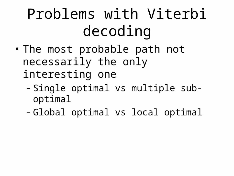
Problems with Viterbi decoding
• The most probable path not necessarily the only interesting one– Single optimal vs multiple sub-optimal– Global optimal vs local optimal
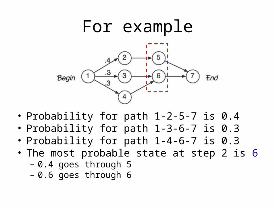
For example
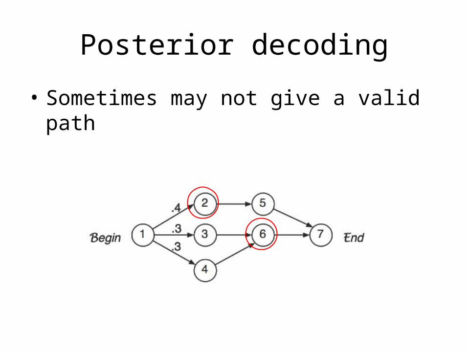
• Probability for path 1-2-5-7 is 0.4• Probability for path 1-3-6-7 is 0.3• Probability for path 1-4-6-7 is 0.3• The most probable state at step 2 is 6
– 0.4 goes through 5– 0.6 goes through 6
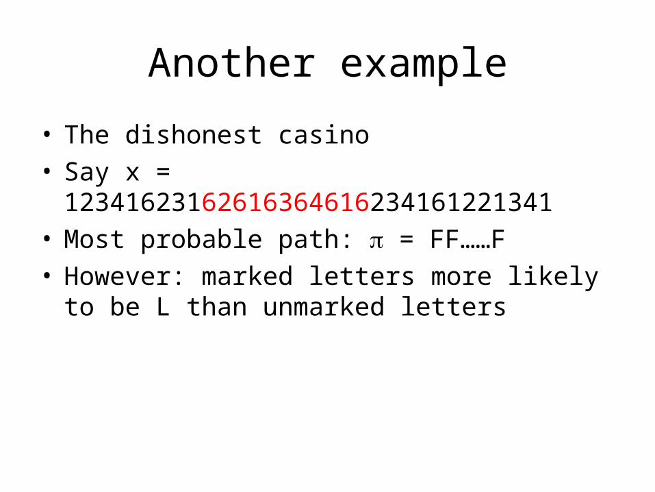
Another example
• The dishonest casino• Say x = 12341623162616364616234161221341• Most probable path: = FF……F• However: marked letters more likely to be L than
unmarked letters
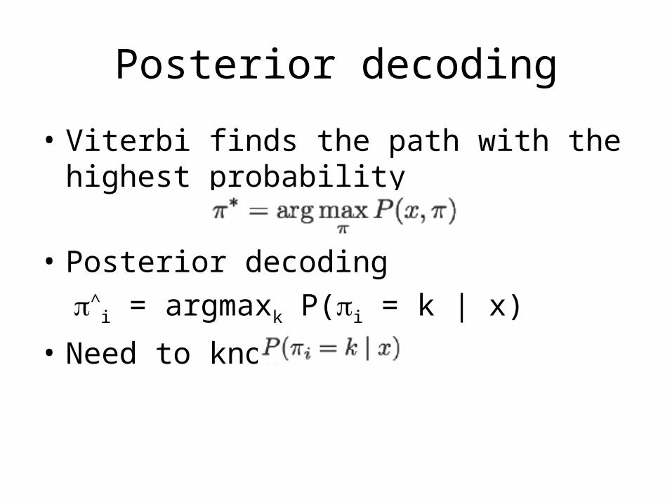
Posterior decoding
• Viterbi finds the path with the highest probability
• Posterior decoding
^i = argmaxk P(i = k | x)
• Need to know

Posterior decoding
• In order to do posterior decoding, we need to know the probability of a sequence given a model, since
• This is called the evaluation problem
• The solution: Forward-backward algorithm

The forward algorithm

Relation between Forward and Viterbi
VITERBI
Initialization:
P0(0) = 1
Pk(0) = 0, for all k > 0
Iteration:
Pk(i) = ek(xi) maxj Pj(i-1) ajk
Termination:
Prob(x, *) = maxk Pk(N)
FORWARD
Initialization:
f0(0) = 1
fk(0) = 0, for all k > 0
Iteration:
fk(i) = ek(xi) j fj(i-1) ajk
Termination:
Prob(x) = k fk(N)

1
This does not include the emission probability of xi

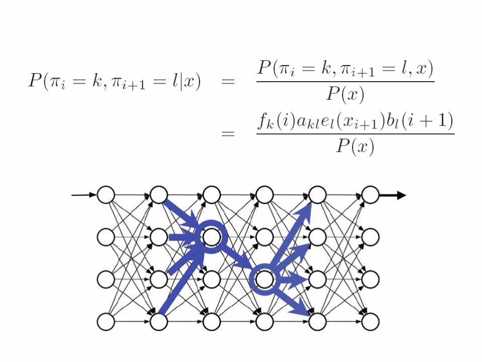
Forward-backward algorithm
• fk(i): prob to get to pos i in state k and emit xi
• bk(i): prob from i to end, given i is in state k
• What is fk(i) bk(i)?– Answer:
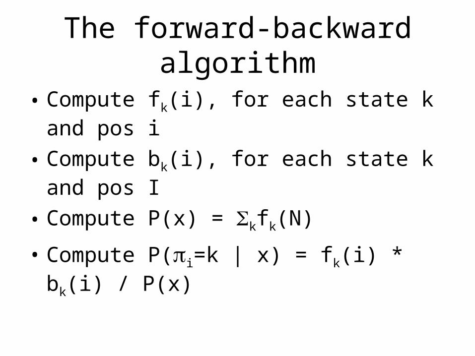
The forward-backward algorithm
• Compute fk(i), for each state k and pos i
• Compute bk(i), for each state k and pos I
• Compute P(x) = kfk(N)
• Compute P(i=k | x) = fk(i) * bk(i) / P(x)
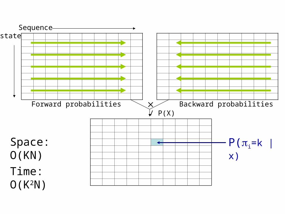
stateSequence
P(i=k | x)Space: O(KN)
Time: O(K2N)
/ P(X)Forward probabilities Backward probabilities

The Forward-backward algorithm
• Posterior decoding
^i = argmaxk P(i = k | x)
• Confidence level for the assignment
• Similarly idea can be used to compute
P(i = k, i+1 = l | x): the probability that a
particular transition is used

For example
If P(fair) > 0.5, the roll is more likely to be generated by a fair die than a loaded die
Posterior decoding
• Sometimes may not give a valid path

Today
• Learning
• Practical issues in HMM learning

What if a new genome comes?We just sequenced the porcupine genome
We know CpG islands play the same role in this genome
However, we have no known CpG islands for porcupines
We suspect the frequency and characteristics of CpG islands are quite different in porcupines
How do we adjust the parameters in our model?
- LEARNING
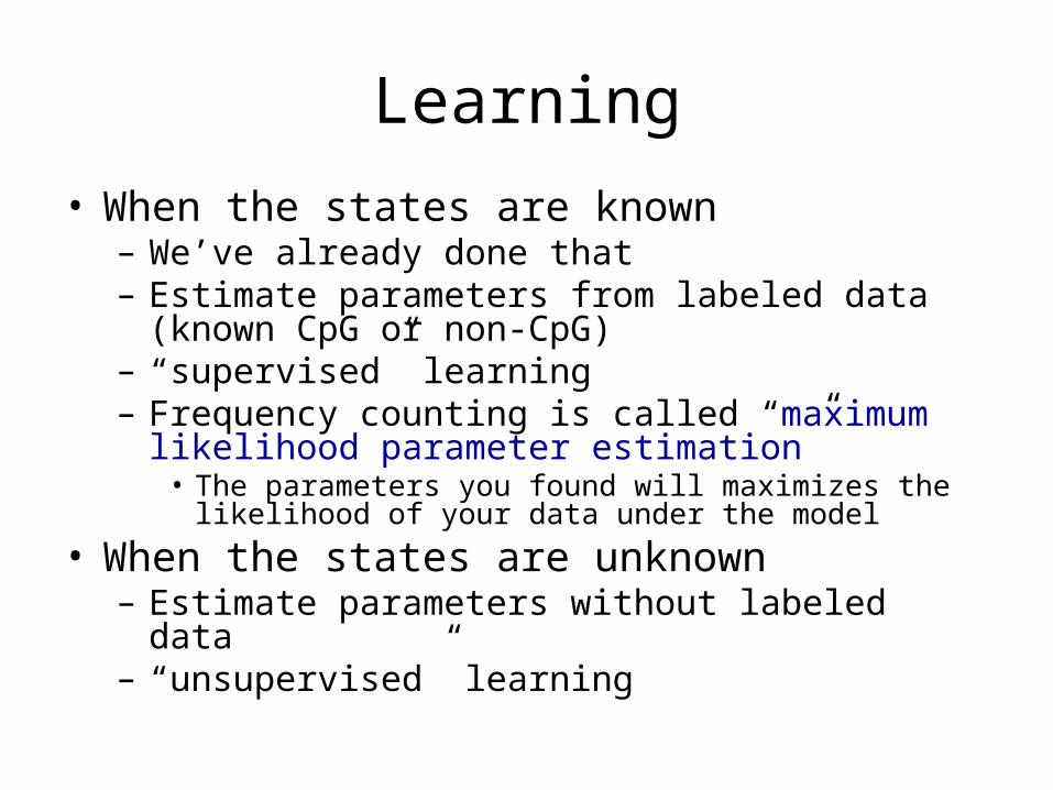
Learning
• When the states are known– We’ve already done that– Estimate parameters from labeled data (known CpG
or non-CpG)– “supervised” learning– Frequency counting is called “maximum likelihood
parameter estimation”• The parameters you found will maximizes the likelihood of
your data under the model
• When the states are unknown– Estimate parameters without labeled data– “unsupervised” learning

Basic idea
1. We estimate our “best guess” on the model parameters θ
2. We use θ to predict the unknown labels
3. We re-estimate a new set of θ
4. Repeat 2 & 3
Two ways
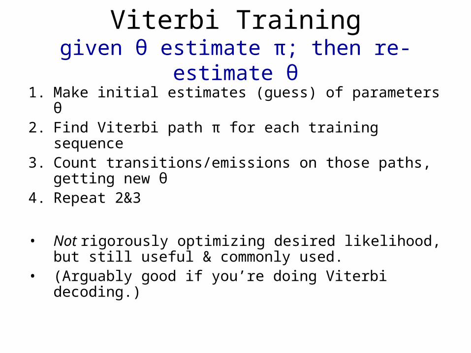
Viterbi Traininggiven θ estimate π; then re-estimate θ
1. Make initial estimates (guess) of parameters θ2. Find Viterbi path π for each training sequence3. Count transitions/emissions on those paths,
getting new θ4. Repeat 2&3
• Not rigorously optimizing desired likelihood, but still useful & commonly used.
• (Arguably good if you’re doing Viterbi decoding.)

Baum-Welch Traininggiven θ, estimate π ensemble; then re-estimate θ
• Instead of estimating the new θ from the most probable path
• We can re-estimate θ from all possible paths– For example, according to Viterbi, pos i is in state k
and pos (i+1) is in state l– This contributes 1 count towards the frequency that
transition kl is used– In Baum-Welch, this transition is counted only
partially, according to the probability that this transition is taken by some path
– Similar for emission

Question
• How to compute
P(i = k, i = l | X)?
• Evaluation problem– Solvable with the backward-forward algorithm
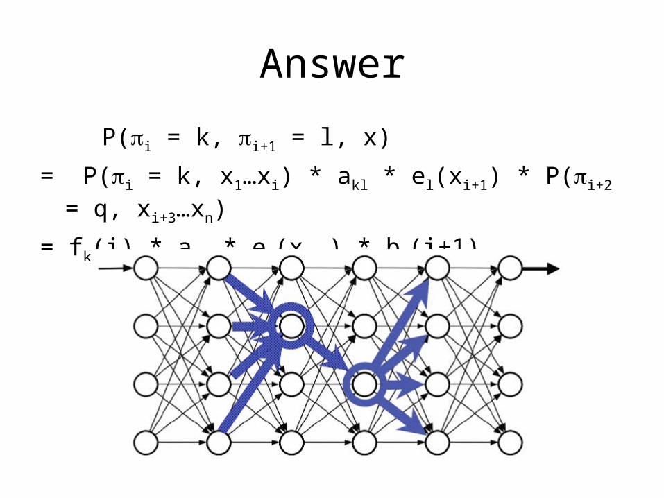
Answer
P(i = k, i+1 = l, x)
= P(i = k, x1…xi) * akl * el(xi+1) * P(i+2 = q, xi+3…xn)
= fk(i) * akl * el(xi+1) * bl(i+1)

Estimated # of kl transition:
New transition probabilities:
Estimated # of symbol t emitted in state k:
New emission probabilities:

Why is this working?
• Proof is very technical (chap 11 in Durbin book)• But basically,
– The backward-forward algorithm computes the likelihood of the data P(X | θ)
– When we re-estimate θ, we maximize P(X | θ).– Effect: in each iteration, the likelihood of the sequence
will be improved– Therefore, guaranteed to converge (not necessarily to
a global optimal)– Viterbi training is also guaranteed to converge: every
iteration we improve the probability of the most probable path

Expectation-maximization (EM)
• Baum-Welch algorithm is a special case of the expectation-maximization (EM) algorithm, a widely used technique in statistics for learning parameters from unlabeled data
• E-step: compute the expectation (e.g. prob for each pos to be in a certain state)
• M-step: maximum-likelihood parameter estimation
• We’ll see EM and similar techniques again in motif finding
• k-means clustering is a special case of EM

Does it actually work?
Depend on:• Nature of the problem• Quality of model (architecture)• Size of training data• Selection of initial parameters
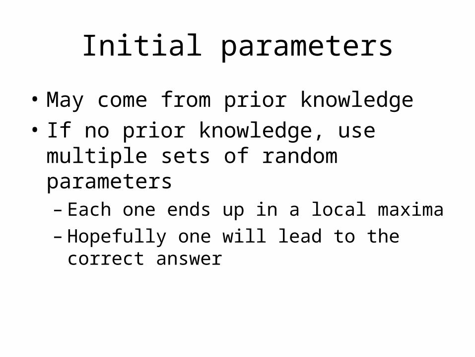
Initial parameters
• May come from prior knowledge
• If no prior knowledge, use multiple sets of random parameters– Each one ends up in a local maxima– Hopefully one will lead to the correct answer
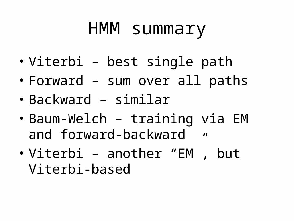
HMM summary
• Viterbi – best single path
• Forward – sum over all paths
• Backward – similar
• Baum-Welch – training via EM and forward-backward
• Viterbi – another “EM”, but Viterbi-based

HMM structure
• We have assumed a fully connected structure– In practice, many transitions are impossible or have very low
probabilities
• “Let the model find out for itself” which transition to use– Almost never work in practice– Poor model even with plenty of training data– Too many local optima when not constrained
• Most successful HMMs are based on knowledge– Model topology should have an interpretation– Some standard topology to choose in typical situations
• Define the model as well as you can– Model surgery based on data

Duration modeling
• For any sub-path, the probability consists of two components– The product of emission probabilities
• Depend on symbols and state path
– The product of transition probabilities• Depend on state path
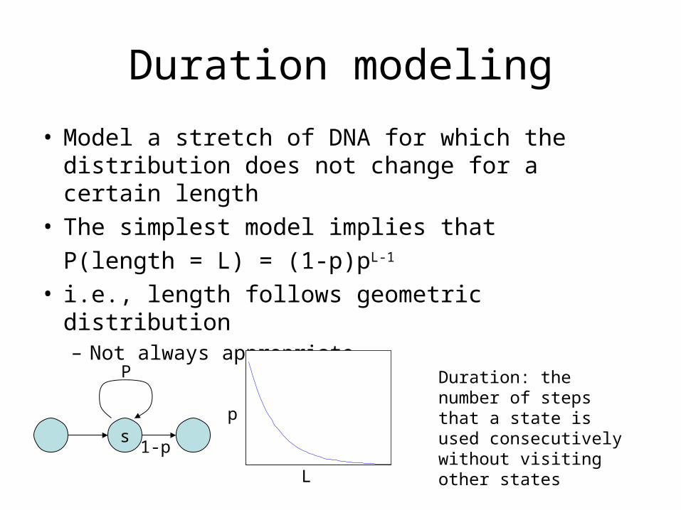
Duration modeling
• Model a stretch of DNA for which the distribution does not change for a certain length
• The simplest model implies that
P(length = L) = (1-p)pL-1
• i.e., length follows geometric distribution– Not always appropriate
s
P
1-p
Duration: the number of steps that a state is used consecutively without visiting other states
L
p

Duration models
s
P
s ss
s
P
s ss
1-p
Negative binominal
Min, then geometric
1-p
PPP
1-p1-p1-p

Explicit duration modeling
Intron
P(A | I) = 0.3P(C | I) = 0.2P(G | I) = 0.2P(T | I) = 0.3
L
P
Exon Intergenic
Empirical intron length distribution

Explicit duration modeling• Can use any arbitrary length distribution• Generalized HMM. Often used in gene finders
Upon entering a state:
1. Choose duration d, according to probability distribution2. Generate d letters according to emission probs3. Take a transition to next state according to transition probs
Pk(i) = maxl maxd=1..D Pl(i-d) alk ek(i-d+1, …, i) P (length = d in state k)
Disadvantage: Increase in complexity:Time: O(D2)Space: O(D)
Where D = maximum duration of state

Silent states
• Silent states are states that do not emit symbols (e.g., the state 0 in our previous examples)
• Silent states can be introduced in HMMs to reduce the number of transitions

Silent states
• Suppose we want to model a sequence in which arbitrary deletions are allowed (in next lecture)
• In that case we need some completely forward connected HMM (O(m2) edges)

Silent states
• If we use silent states, we use only O(m) edges
• Nothing comes freeSuppose we want to assign high probability to 1→5 and 2→4, there is no way to have also low probability on 1→4and 2→5.
Algorithms can be modified easily to deal with silent states, so long as no silent-state loops

HMM applications
• Pair-wise sequence alignment
• Multiple sequence alignment
• Gene finding
• Speech recognition: a good tutorial on course website
• Machine translation
• Many others
• Connection between HMM and sequence alignments
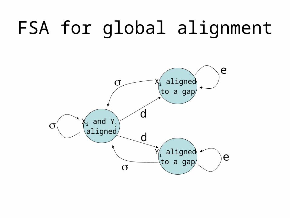
FSA for global alignment
Xi and Yj aligned
Xi aligned to a gap
Yj aligned to a gap
d
d
e
e
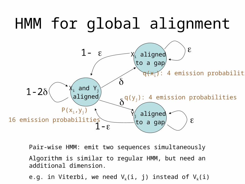
HMM for global alignment
Xi and Yj aligned
Xi aligned to a gap
Yj aligned to a gap
1-2
1-
1-
Pair-wise HMM: emit two sequences simultaneously
Algorithm is similar to regular HMM, but need an additional dimension.
e.g. in Viterbi, we need Vk(i, j) instead of Vk(i)
P(xi,yj)
16 emission probabilities
q(xi): 4 emission probabilities
q(yj): 4 emission probabilities

HMM and FSA for alignment
• FSA: regular grammar• HMM: stochastic regular grammar• After proper transformation between the
probabilities and substitution scores, the two are identical (a, b) log [p(a, b) / (q(a) q(b))] d log e log
• Details in Durbin book chap 4• Finding an optimal FSA alignment is equivalent
to finding the most probable path with Viterbi

HMM for pair-wise alignment
• Theoretical advantages:– Full probabilistic interpretation of alignment scores– Probability of all alignments instead of the best
alignment (forward-backward alignment)– Sampling sub-optimal alignments
– Posterior probability that Ai is aligned to Bj
• Not commonly used in practice– Needleman-Wunsch and Smith-Waterman algorithms
work pretty well, and more intuitive to biologists– Other reasons?
Next lecture
• HMM for multiple alignment– Very useful
• HMM for gene finding– Very useful– But very technical– Include many knowledge-based fine-tunes
and extensions– We’ll only discuss basic ideas