cs489-02 & cs589-02 multimedia processing lecture 2. intensity transformation and spatial...
TRANSCRIPT

CS489-02 & CS589-02 Multimedia Processing
Lecture 2. Intensity Transformation and Spatial
Filtering
Spring 2009
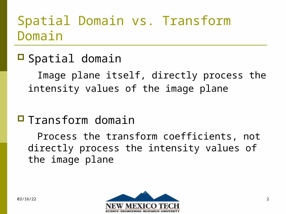
Spatial Domain vs. Transform Domain
Spatial domain Image plane itself, directly process the intensity
values of the image plane
Transform domain Process the transform coefficients, not directly
process the intensity values of the image plane
04/18/23 2
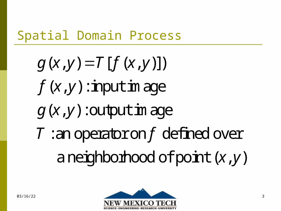
Spatial Domain Process
04/18/23 3
( , ) [ ( , )])
( , ) : input image
( , ) : output image
: an operator on defined over
a neighborhood of point ( , )
g x y T f x y
f x y
g x y
T f
x y
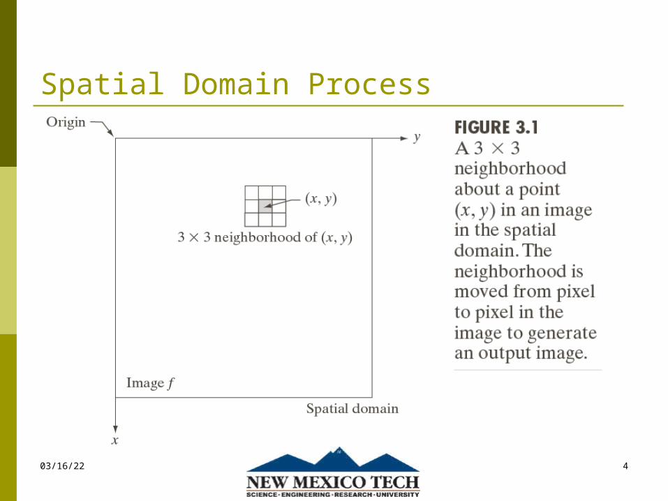
Spatial Domain Process
04/18/23 4
Spatial Domain Process
04/18/23 5
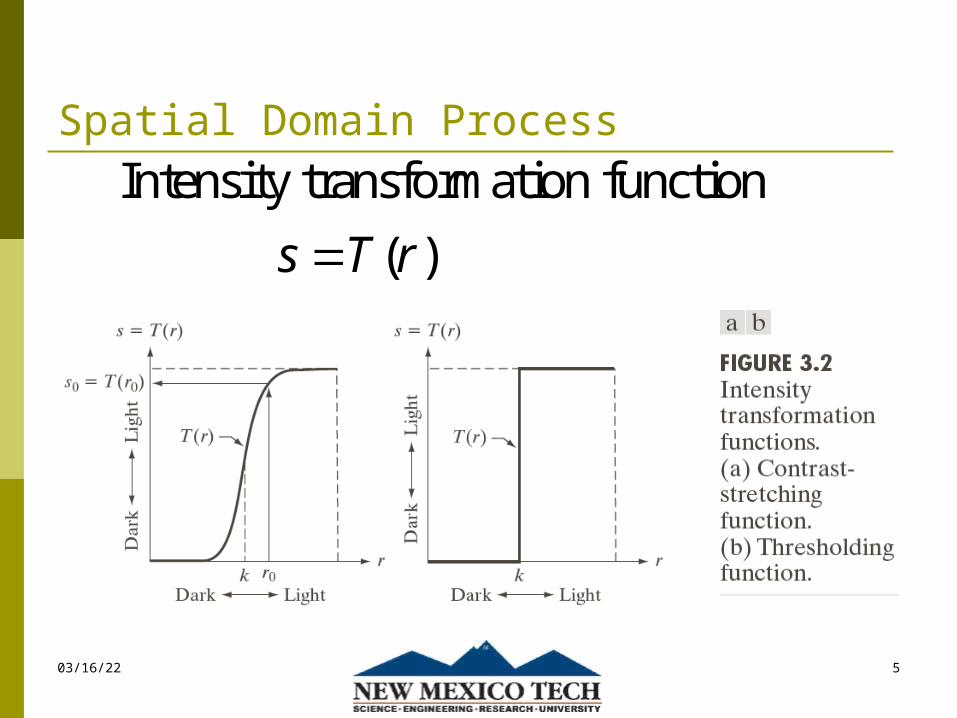
Intensity transformation function
( )s T r

Some Basic Intensity Transformation Functions
04/18/23 6
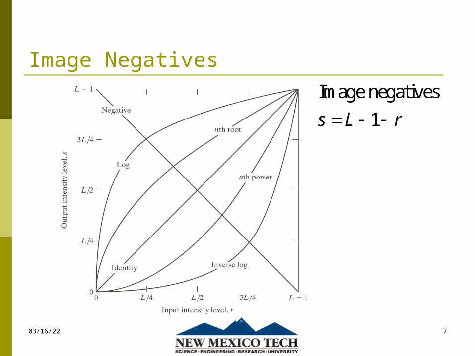
Image Negatives
04/18/23 7
Image negatives
1s L r
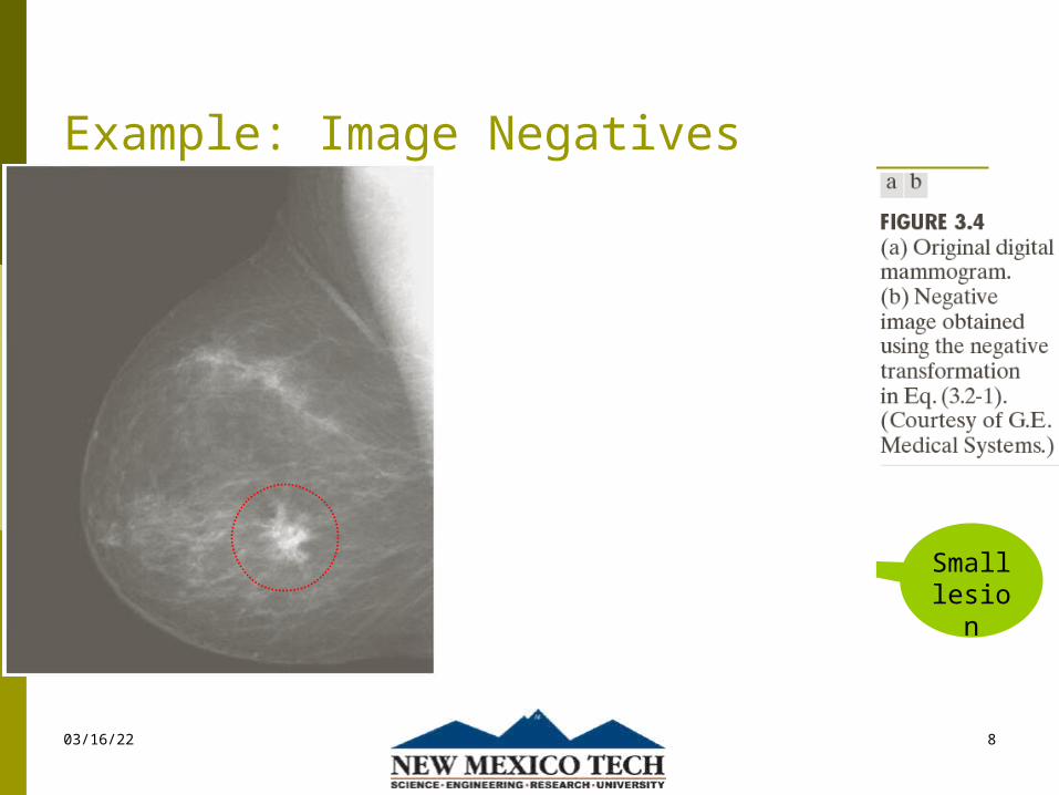
Example: Image Negatives
04/18/23 8
Small lesion

Log Transformations
04/18/23 9
Log Transformations
log(1 )s c r

Example: Log Transformations
04/18/23 10

Power-Law (Gamma) Transformations
04/18/23 11
s cr

Example: Gamma Transformations
04/18/23 12
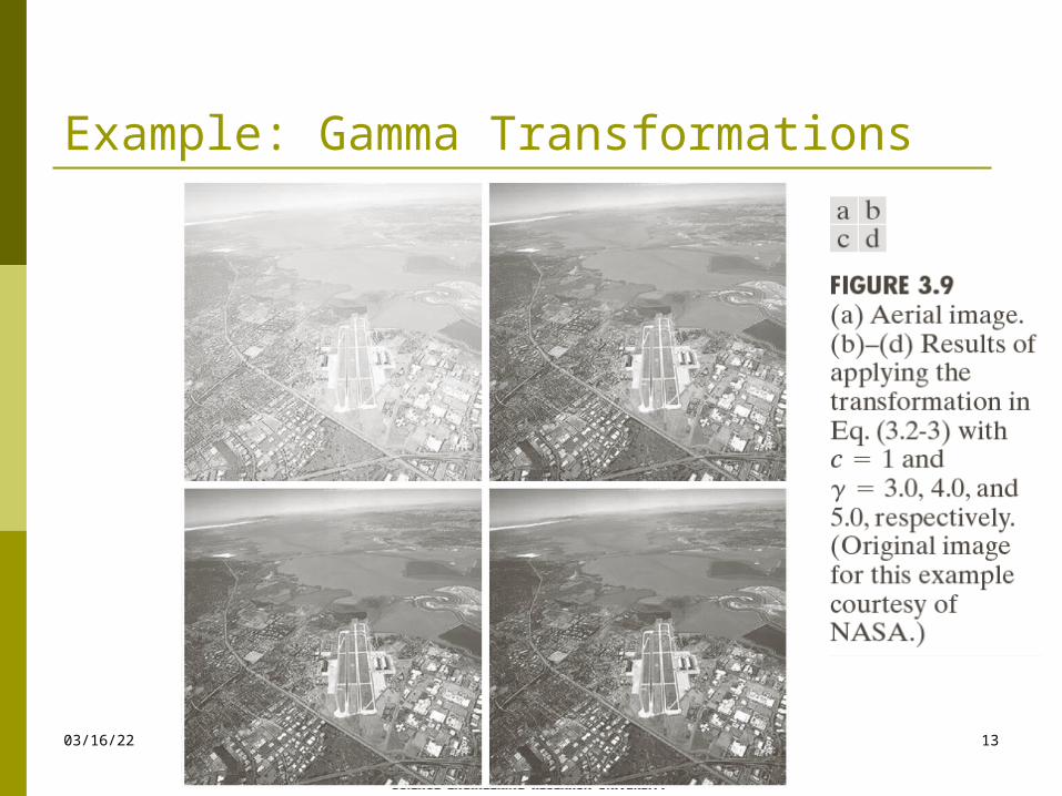
Example: Gamma Transformations
04/18/23 13
Piecewise-Linear Transformations
Contrast Stretching — Expands the range of intensity levels in an image ― spans the full intensity range of the recording medium
Intensity-level Slicing — Highlights a specific range of intensities in an image
04/18/23 14

04/18/23 15

04/18/23 16
Highlight the major blood vessels and study the shape of the flow of the contrast medium (to detect blockages, etc.)
Measuring the actual flow of the contrast medium as a function of time in a series of images

Bit-plane Slicing
04/18/23 17
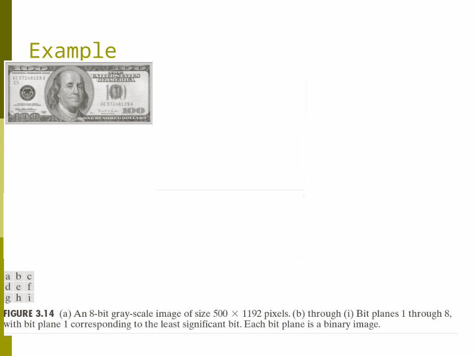
Example
04/18/23 18

Example
04/18/23 19

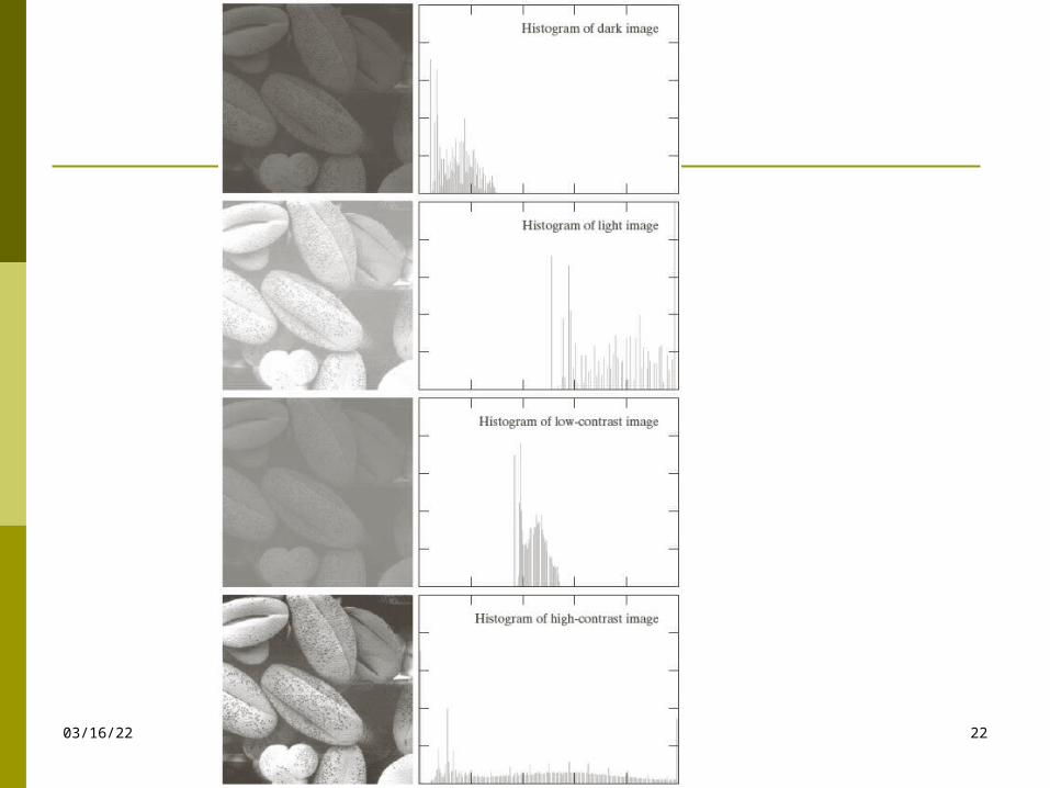
Histogram Processing
Histogram Equalization
Histogram Matching
Local Histogram Processing
Using Histogram Statistics for Image Enhancement
04/18/23 20

Histogram Processing
Normalized histogram ( )
: the number of pixels in the image of
size M N with intensity
kk
k
k
np r
MNn
r
04/18/23 21
Histogram ( )
is the intensity value
is the number of pixels in the image with intensity
k k
thk
k k
h r n
r k
n r
04/18/23 22
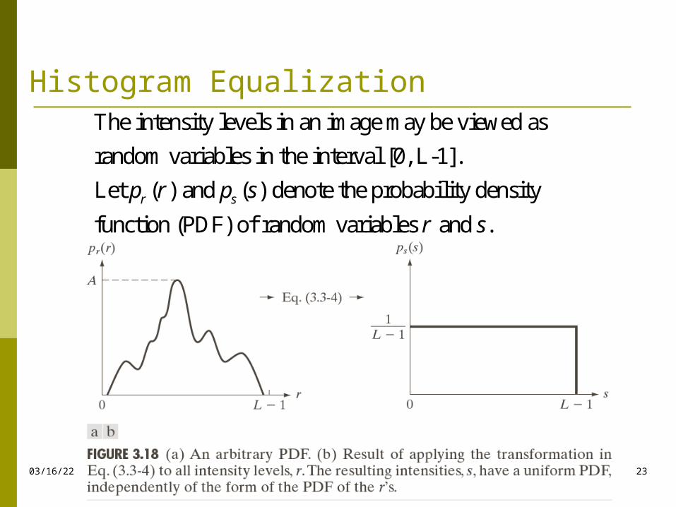
Histogram Equalization
04/18/23 23
The intensity levels in an image may be viewed as
random variables in the interval [0, L-1].
Let ( ) and ( ) denote the probability density
function (PDF) of random variables and .r sp r p s
r s

Histogram Equalization
. T(r) is a strictly monotonically increasing function
in the interval 0 -1;
. 0 ( ) -1 for 0 -1.
a
r L
b T r L r L
04/18/23 24
( ) 0 1s T r r L
Histogram Equalization
. T(r) is a strictly monotonically increasing function
in the interval 0 -1;
. 0 ( ) -1 for 0 -1.
a
r L
b T r L r L
( ) ( )s rp s ds p r dr04/18/23 25
( ) 0 1s T r r L
( ) is continuous and differentiable.T r
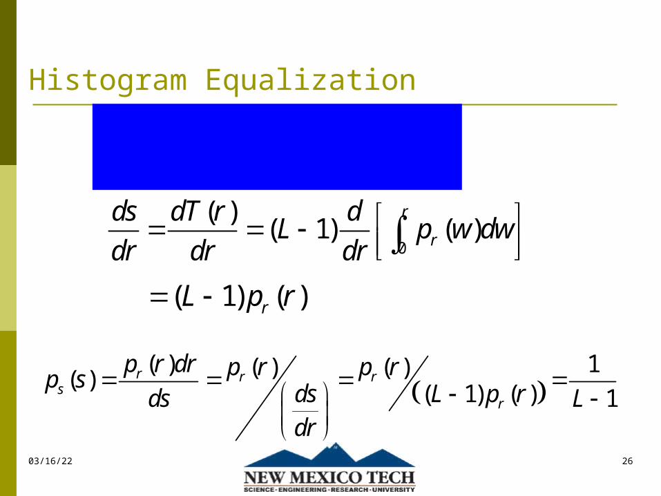
Histogram Equalization
0( ) ( 1) ( )
r
rs T r L p w dw
04/18/23 26
0
( )( 1) ( )
r
r
ds dT r dL p w dw
dr dr dr
( 1) ( )rL p r
( ) 1( ) ( )( )
( 1) ( ) 1r r r
sr
p r dr p r p rp sL p rdsds L
dr

Example
04/18/23 27
2
Suppose that the (continuous) intensity values
in an image have the PDF
2, for 0 r L-1
( 1)( )
0, otherwise
Find the transformation function for equalizing
the image histogra
r
r
Lp r
m.
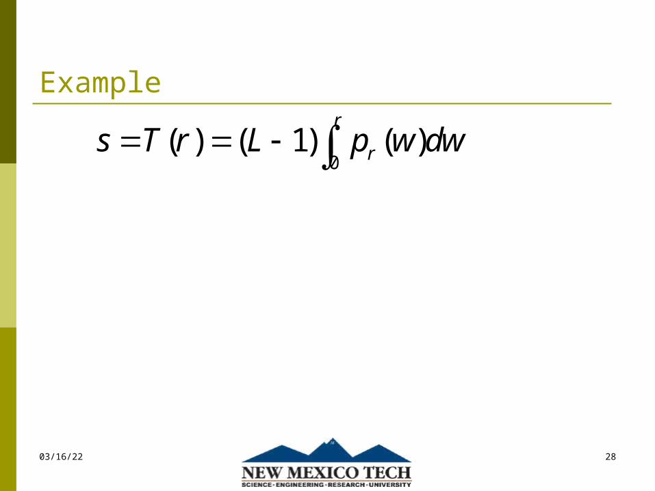
Example
20
2( 1)
( 1)
r wL dw
L
04/18/23 28
0( ) ( 1) ( )
r
rs T r L p w dw
2
1
r
L
Histogram Equalization
0
Continuous case:
( ) ( 1) ( )r
rs T r L p w dw
0
Discrete values:
( ) ( 1) ( )k
k k r jj
s T r L p r
0 0
1( 1) k=0,1,..., L-1
k kj
jj j
n LL n
MN MN
04/18/23 29
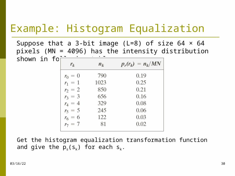
Example: Histogram Equalization
04/18/23 30
Suppose that a 3-bit image (L=8) of size 64 × 64 pixels (MN = 4096) has the intensity distribution shown in following table.
Get the histogram equalization transformation function and give the ps(sk) for each sk.
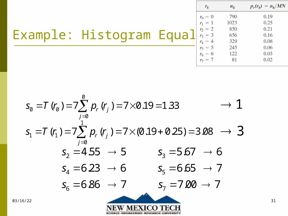
Example: Histogram Equalization
04/18/23 31
0
0 00
( ) 7 ( ) 7 0.19 1.33r jj
s T r p r
11
1 10
( ) 7 ( ) 7 (0.19 0.25) 3.08r jj
s T r p r
3
2 3
4 5
6 7
4.55 5 5.67 6
6.23 6 6.65 7
6.86 7 7.00 7
s s
s s
s s
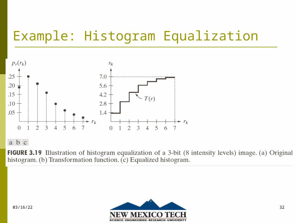
Example: Histogram Equalization
04/18/23 32

04/18/23 33

04/18/23 34

Question Is histogram equalization always good?
No
04/18/23 35
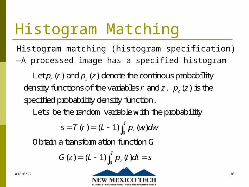
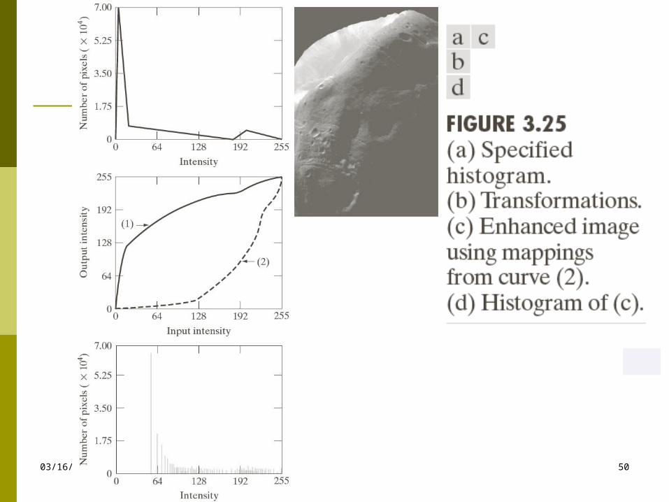
Histogram MatchingHistogram matching (histogram specification) —A processed image has a specified histogram
04/18/23 36
Let ( ) and ( ) denote the continous probability
density functions of the variables and . ( ) is the
specified probability density function.
Let be the random variable with the pro
r z
z
p r p z
r z p z
s
0
0
bability
( ) ( 1) ( )
Obtain a transformation function G
( ) ( 1) ( )
r
r
z
z
s T r L p w dw
G z L p t dt s

Histogram Matching
04/18/23 37
0
0
( ) ( 1) ( )
( ) ( 1) ( )
r
r
z
z
s T r L p w dw
G z L p t dt s
1 1( ) ( )z G s G T r

Histogram Matching: Procedure Obtain pr(r) from the input image and then obtain the
values of s
Use the specified PDF and obtain the transformation function G(z)
Mapping from s to z
0( 1) ( )
r
rs L p w dw
0( ) ( 1) ( )
z
zG z L p t dt s
04/18/23 38
1( )z G s

Histogram Matching: Example
Assuming continuous intensity values, suppose that an image has the intensity PDF
Find the transformation function that will produce an image whose intensity PDF is
2
2, for 0 -1
( 1)( )
0 , otherwiser
rr L
Lp r
04/18/23 39
2
3
3, for 0 ( -1)
( ) ( 1)
0, otherwisez
zz L
p z L

Histogram Matching: Example
Find the histogram equalization transformation for the input image
Find the histogram equalization transformation for the specified histogram
The transformation function
20 0
2( ) ( 1) ( ) ( 1)
( 1)
r r
r
ws T r L p w dw L dw
L
04/18/23 40
2 3
3 20 0
3( ) ( 1) ( ) ( 1)
( 1) ( 1)
z z
z
t zG z L p t dt L dt s
L L
2
1
r
L
1/321/3 1/32 2 2( 1) ( 1) ( 1)
1
rz L s L L r
L
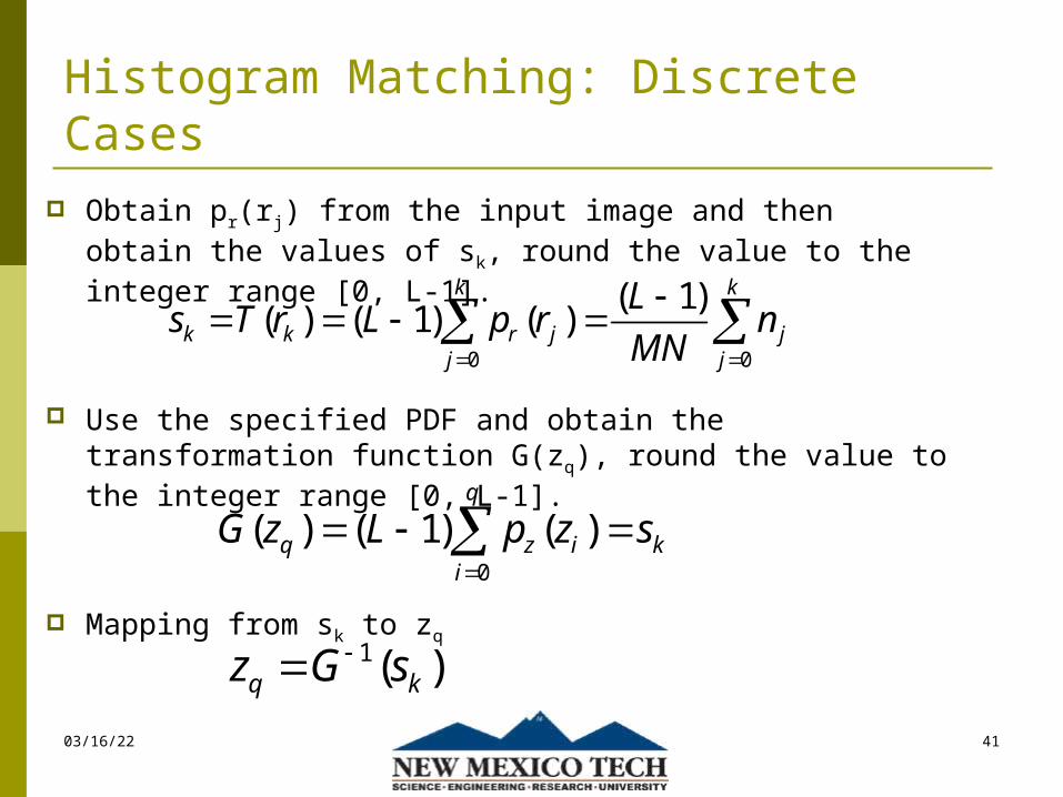
Histogram Matching: Discrete Cases Obtain pr(rj) from the input image and then obtain the
values of sk, round the value to the integer range [0, L-1].
Use the specified PDF and obtain the transformation function G(zq), round the value to the integer range [0, L-1].
Mapping from sk to zq
0 0
( 1)( ) ( 1) ( )
k k
k k r j jj j
Ls T r L p r n
MN
0
( ) ( 1) ( )q
q z i ki
G z L p z s
04/18/23 41
1( )q kz G s

Example: Histogram Matching
04/18/23 42
Suppose that a 3-bit image (L=8) of size 64 × 64 pixels (MN = 4096) has the intensity distribution shown in the following table (on the left). Get the histogram transformation function and make the output image with the specified histogram, listed in the table on the right.
Example: Histogram Matching
04/18/23 43
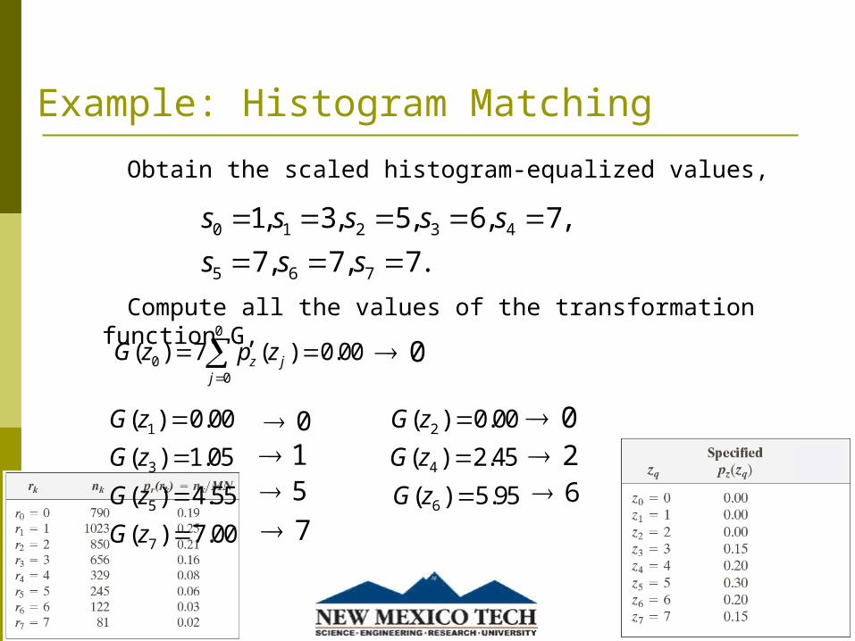
Obtain the scaled histogram-equalized values,
Compute all the values of the transformation function G,
0 1 2 3 4
5 6 7
1, 3, 5, 6, 7,
7, 7, 7.
s s s s s
s s s
0
00
( ) 7 ( ) 0.00z jj
G z p z
1 2
3 4
5 6
7
( ) 0.00 ( ) 0.00
( ) 1.05 ( ) 2.45
( ) 4.55 ( ) 5.95
( ) 7.00
G z G z
G z G z
G z G z
G z
0
0 01 2
657
Example: Histogram Matching
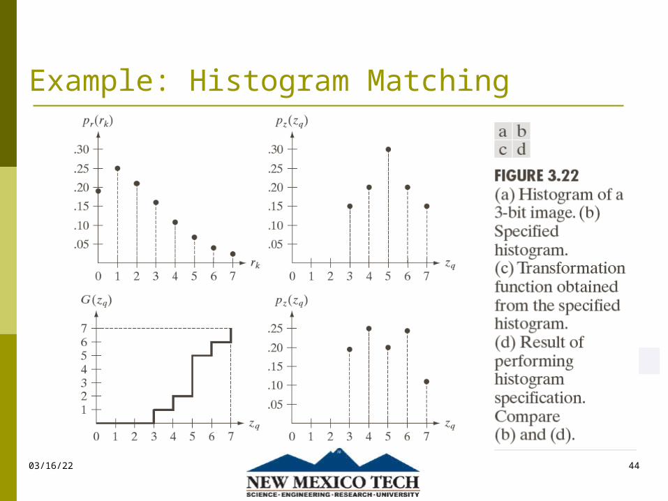
04/18/23 44

Example: Histogram Matching
04/18/23 45
Obtain the scaled histogram-equalized values,
Compute all the values of the transformation function G,
0 1 2 3 4
5 6 7
1, 3, 5, 6, 7,
7, 7, 7.
s s s s s
s s s
0
00
( ) 7 ( ) 0.00z jj
G z p z
1 2
3 4
5 6
7
( ) 0.00 ( ) 0.00
( ) 1.05 ( ) 2.45
( ) 4.55 ( ) 5.95
( ) 7.00
G z G z
G z G z
G z G z
G z
0
0 01 2
657
s0
s2 s3
s5 s6 s7
s1
s4

Example: Histogram Matching
0 1 2 3 4
5 6 7
1, 3, 5, 6, 7,
7, 7, 7.
s s s s s
s s s
04/18/23 46
0
1
2
3
4
5
6
7
kr
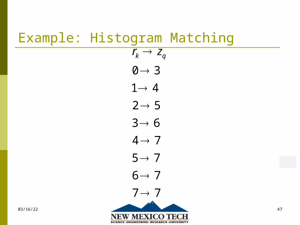
Example: Histogram Matching
04/18/23 47
0 3
1 4
2 5
3 6
4 7
5 7
6 7
7 7
k qr z

Example: Histogram Matching
04/18/23 48
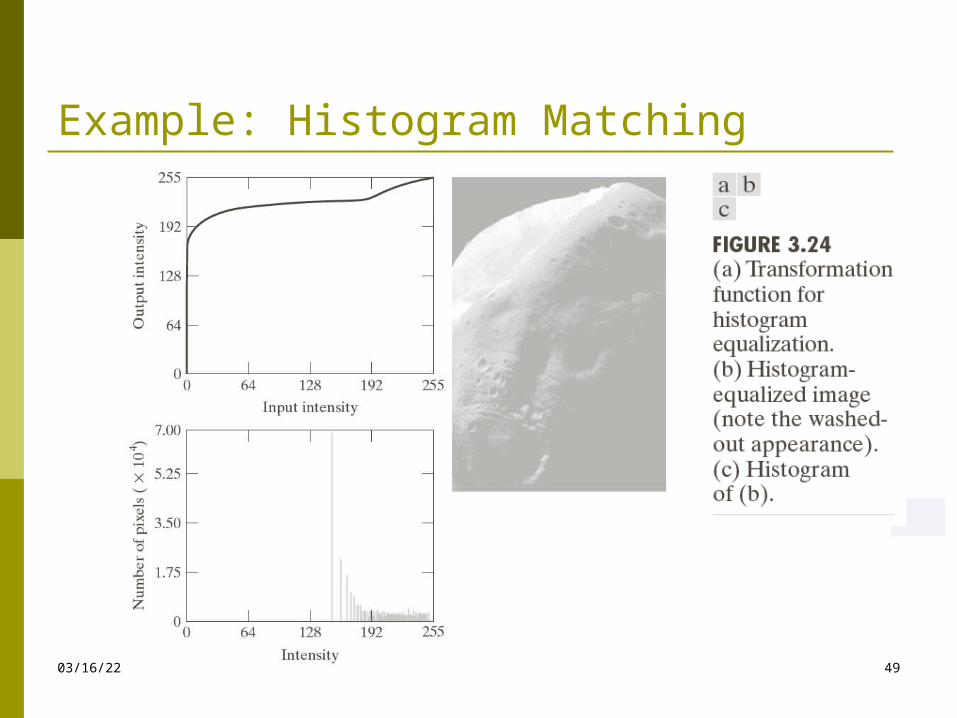
Example: Histogram Matching
04/18/23 49
04/18/23 50
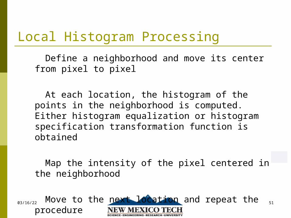
Local Histogram Processing
04/18/23 51
Define a neighborhood and move its center from pixel to pixel
At each location, the histogram of the points in the neighborhood is computed. Either histogram equalization or histogram specification transformation function is obtained
Map the intensity of the pixel centered in the neighborhood
Move to the next location and repeat the procedure
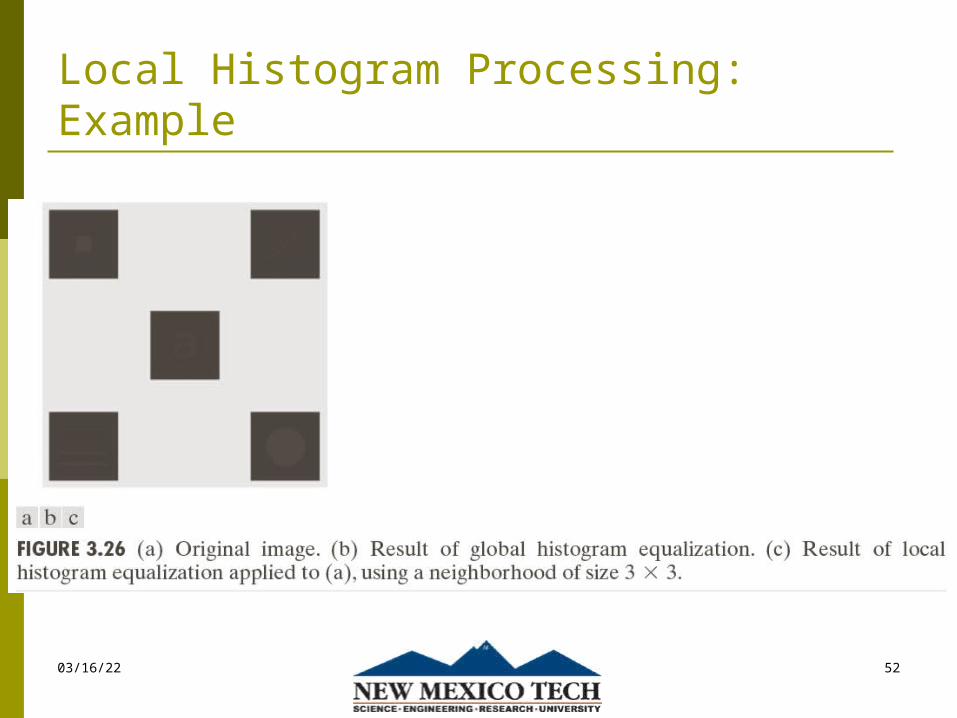
Local Histogram Processing: Example
04/18/23 52
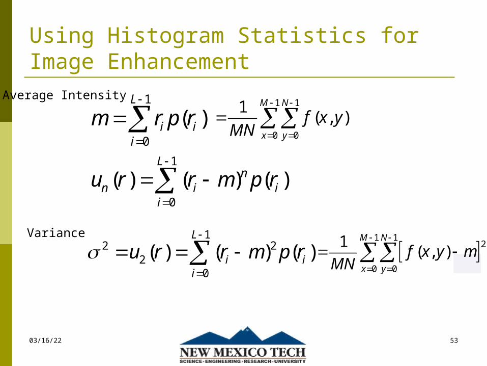
Using Histogram Statistics for Image Enhancement
12 2
20
( ) ( ) ( )L
i ii
u r r m p r
04/18/23 53
1
0
( )L
i ii
m r p r
1
0
( ) ( ) ( )L
nn i i
i
u r r m p r
1 1
0 0
1( , )
M N
x y
f x yMN
1 1
2
0 0
1( , )
M N
x y
f x y mMN
Average Intensity
Variance
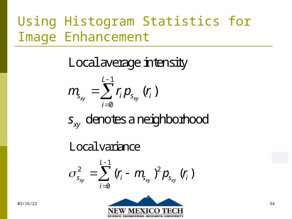
Using Histogram Statistics for Image Enhancement
12 2
0
Local variance
( ) ( )xy xy xy
L
s i s s ii
r m p r
04/18/23 54
1
0
Local average intensity
( )
denotes a neighborhood
xy xy
L
s i s ii
xy
m r p r
s
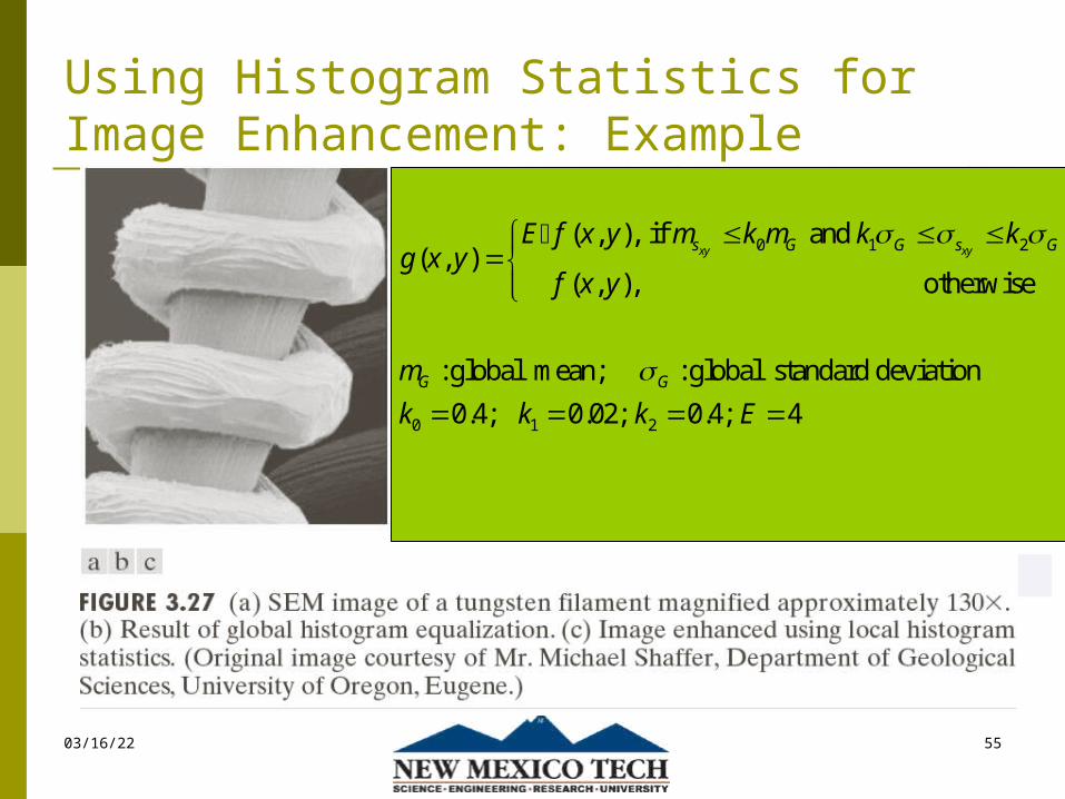
Using Histogram Statistics for Image Enhancement: Example
04/18/23 55
0 1 2
0 1 2
( , ), if and ( , )
( , ), otherwise
: global mean; : global standard deviation
0.4; 0.02; 0.4; 4
xy xys G G s G
G G
E f x y m k m k kg x y
f x y
m
k k k E

Spatial Filtering
04/18/23 56
A spatial filter consists of (a) a neighborhood, and (b) a predefined operation
Linear spatial filtering of an image of size MxN with a filter of size mxn is given by the expression
( , ) ( , ) ( , )
2 1; 2 1
a b
s a t b
g x y w s t f x s y t
m a n b

Spatial Filtering
04/18/23 57
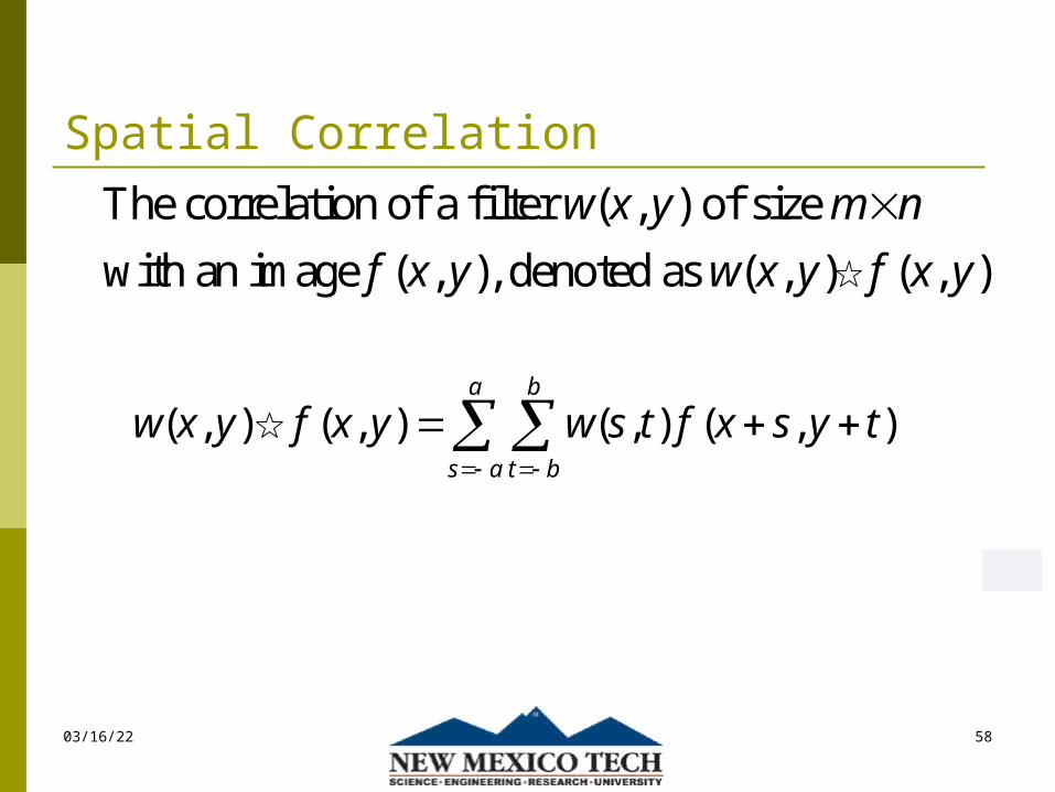
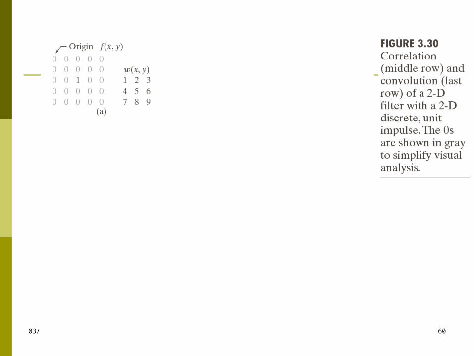
Spatial Correlation
04/18/23 58
The correlation of a filter ( , ) of size
with an image ( , ), denoted as ( , ) ( , )
w x y m n
f x y w x y f x y
( , ) ( , ) ( , ) ( , )a b
s a t b
w x y f x y w s t f x s y t

Spatial Convolution
04/18/23 59
The convolution of a filter ( , ) of size
with an image ( , ), denoted as ( , ) ( , )
w x y m n
f x y w x y f x y
( , ) ( , ) ( , ) ( , )a b
s a t b
w x y f x y w s t f x s y t
04/18/23 60
Smoothing Spatial Filters
04/18/23 61
Smoothing filters are used for blurring and for noise reduction
Blurring is used in removal of small details and bridging of small gaps in lines or curves
Smoothing spatial filters include linear filters and nonlinear filters.
Spatial Smoothing Linear Filters
04/18/23 62
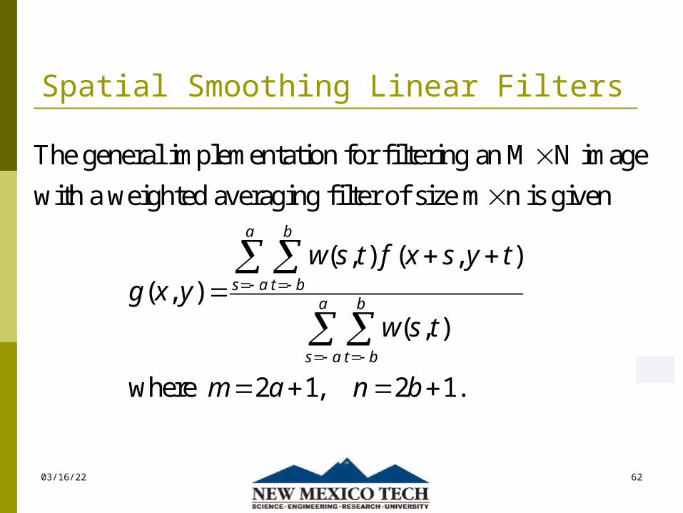
The general implementation for filtering an M N image
with a weighted averaging filter of size m n is given
( , ) ( , ) ( , )
( , )
where 2 1
a b
s a t ba b
s a t b
w s t f x s y tg x y
w s t
m a
, 2 1.n b
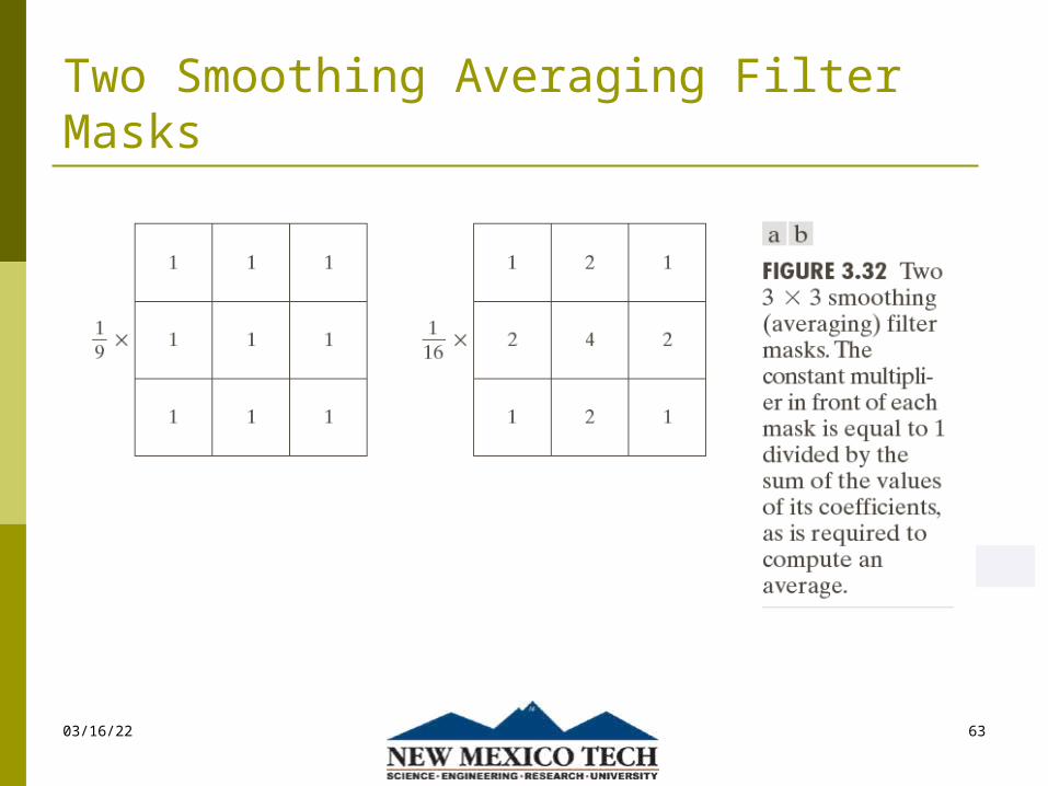
Two Smoothing Averaging Filter Masks
04/18/23 63

04/18/23 64
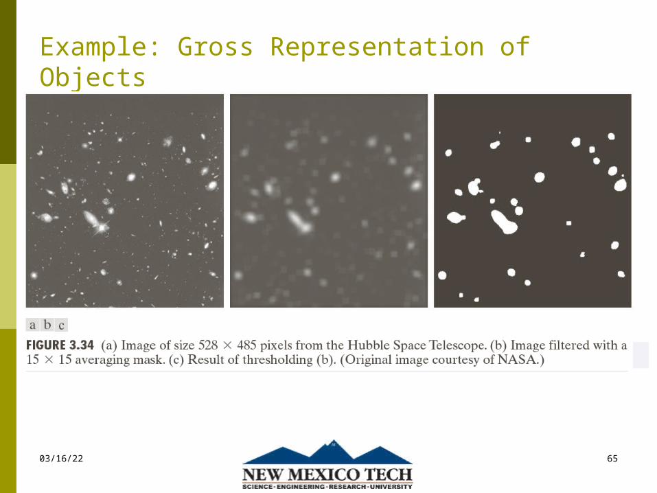
Example: Gross Representation of Objects
04/18/23 65
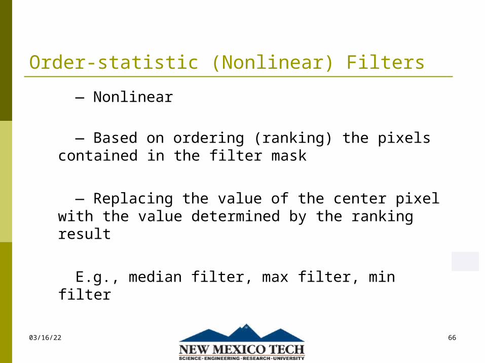
Order-statistic (Nonlinear) Filters
04/18/23 66
— Nonlinear
— Based on ordering (ranking) the pixels contained in the filter mask
— Replacing the value of the center pixel with the value determined by the ranking result
E.g., median filter, max filter, min filter
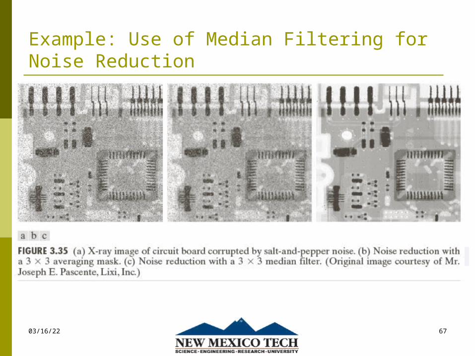
Example: Use of Median Filtering for Noise Reduction
04/18/23 67
Sharpening Spatial Filters
04/18/23 68
► Foundation
► Laplacian Operator
► Unsharp Masking and Highboost Filtering
► Using First-Order Derivatives for Nonlinear Image Sharpening

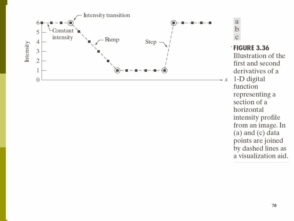
Sharpening Spatial Filters: Foundation
04/18/23 69
► The first-order derivative of a one-dimensional function f(x) is the difference
► The second-order derivative of f(x) as the difference
( 1) ( )f
f x f xx
2
2( 1) ( 1) 2 ( )
ff x f x f x
x
04/18/23 70
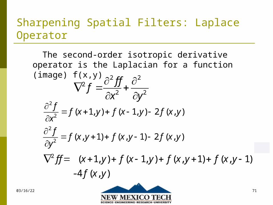
Sharpening Spatial Filters: Laplace Operator
2
2( , 1) ( , 1) 2 ( , )
ff x y f x y f x y
y
04/18/23 71
The second-order isotropic derivative operator is the Laplacian for a function (image) f(x,y)
2 22
2 2
f ff
x y
2
2( 1, ) ( 1, ) 2 ( , )
ff x y f x y f x y
x
2 ( 1, ) ( 1, ) ( , 1) ( , 1)
- 4 ( , )
f f x y f x y f x y f x y
f x y

Sharpening Spatial Filters: Laplace Operator
04/18/23 72
Sharpening Spatial Filters: Laplace Operator
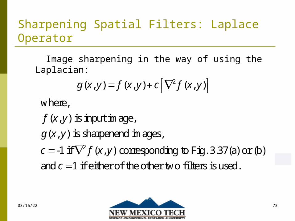
04/18/23 73
Image sharpening in the way of using the Laplacian:
2
2
( , ) ( , ) ( , )
where,
( , ) is input image,
( , ) is sharpenend images,
-1 if ( , ) corresponding to Fig. 3.37(a) or (b)
and 1 if either of the other two filters is us
g x y f x y c f x y
f x y
g x y
c f x y
c
ed.
04/18/23 74

Unsharp Masking and Highboost Filtering
04/18/23 75
► Unsharp masking Sharpen images consists of subtracting an unsharp
(smoothed) version of an image from the original image e.g., printing and publishing industry
► Steps
1. Blur the original image
2. Subtract the blurred image from the original
3. Add the mask to the original
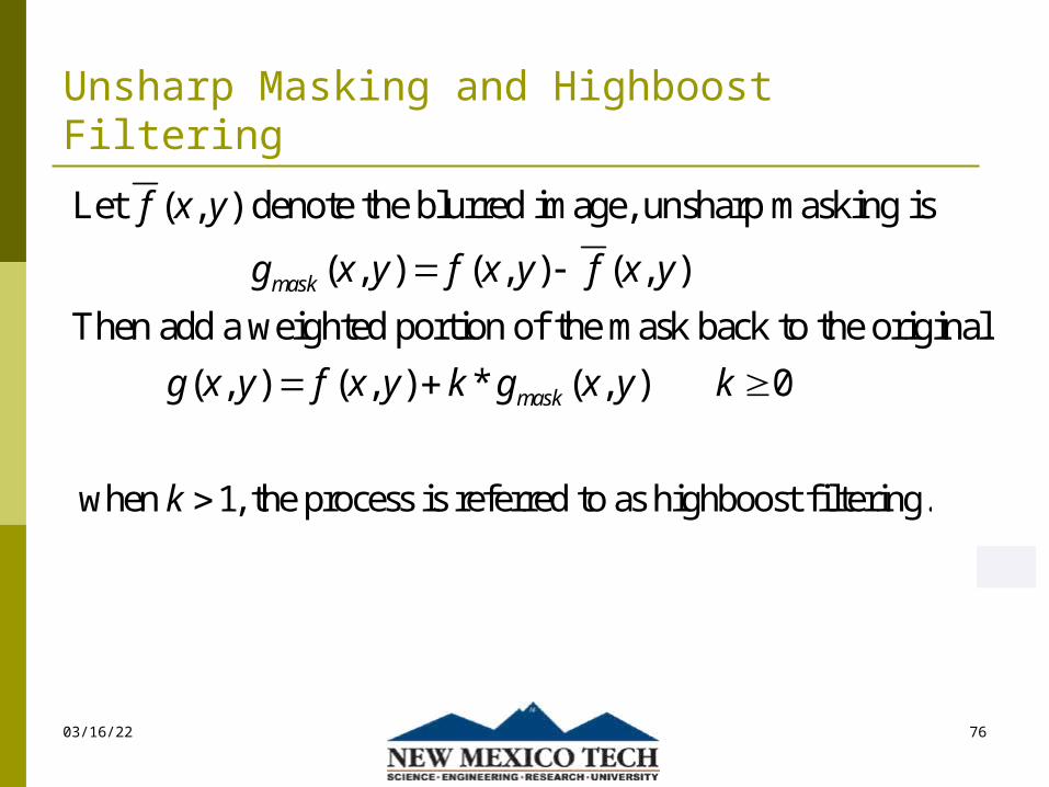
Unsharp Masking and Highboost Filtering
04/18/23 76
Let ( , ) denote the blurred image, unsharp masking is
( , ) ( , ) ( , )
Then add a weighted portion of the mask back to the original
( , ) ( , ) * ( , )
mask
mask
f x y
g x y f x y f x y
g x y f x y k g x y
0k
when 1, the process is referred to as highboost filtering.k
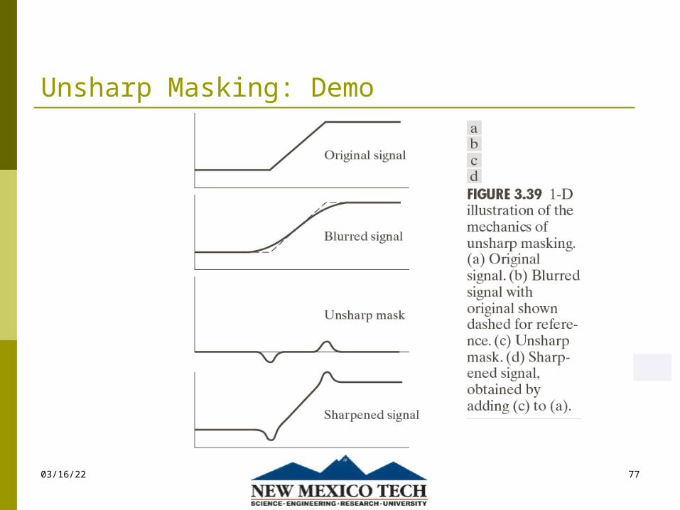
Unsharp Masking: Demo
04/18/23 77
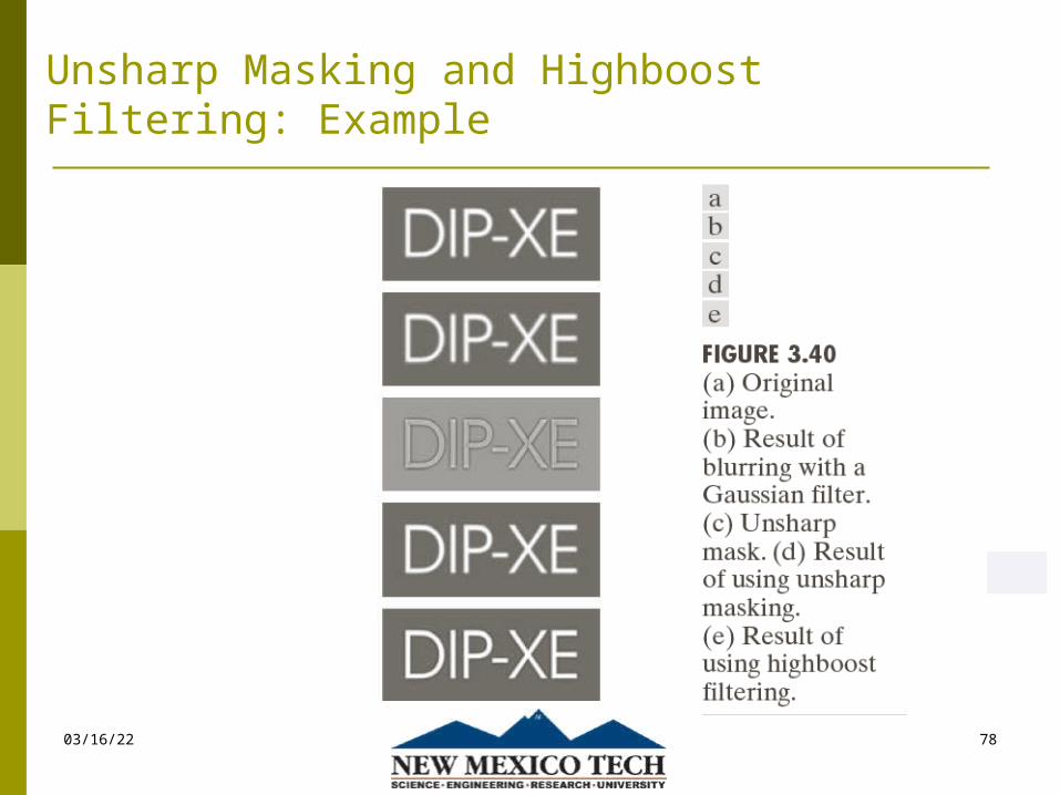
Unsharp Masking and Highboost Filtering: Example
04/18/23 78

Image Sharpening based on First-Order Derivatives
04/18/23 79
For function ( , ), the gradient of at coordinates ( , )
is defined as
grad( ) x
y
f x y f x y
fg x
f ffgy
2 2
The of vector , denoted as ( , )
( , ) mag( ) x y
magnitude f M x y
M x y f g g
Gradient Image
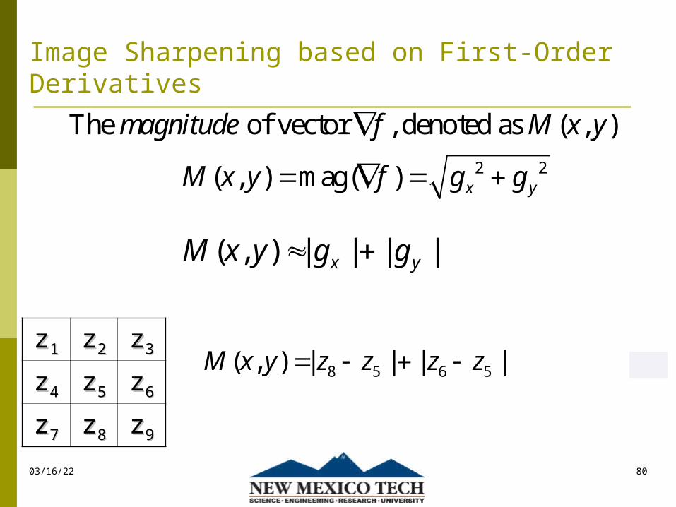
Image Sharpening based on First-Order Derivatives
zz11 zz22 zz33
zz44 zz55 zz66
zz77 zz88 zz99
04/18/23 80
2 2
The of vector , denoted as ( , )
( , ) mag( ) x y
magnitude f M x y
M x y f g g
( , ) | | | |x yM x y g g
8 5 6 5( , ) | | | |M x y z z z z
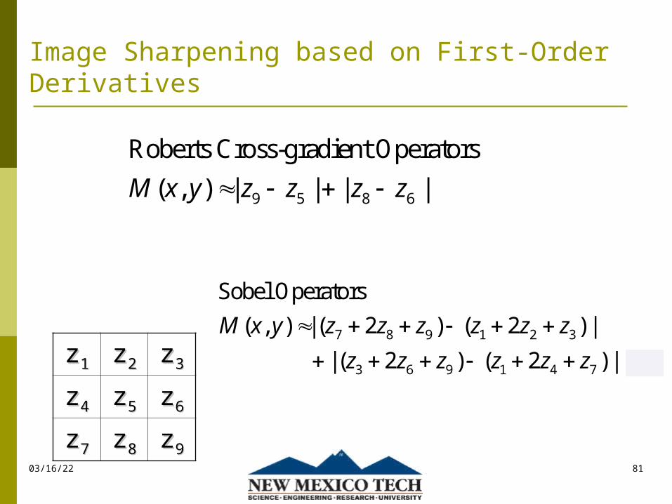
Image Sharpening based on First-Order Derivatives
zz11 zz22 zz33
zz44 zz55 zz66
zz77 zz88 zz9904/18/23 81
9 5 8 6
Roberts Cross-gradient Operators
( , ) | | | |M x y z z z z
7 8 9 1 2 3
3 6 9 1 4 7
Sobel Operators
( , ) | ( 2 ) ( 2 ) |
| ( 2 ) ( 2 ) |
M x y z z z z z z
z z z z z z
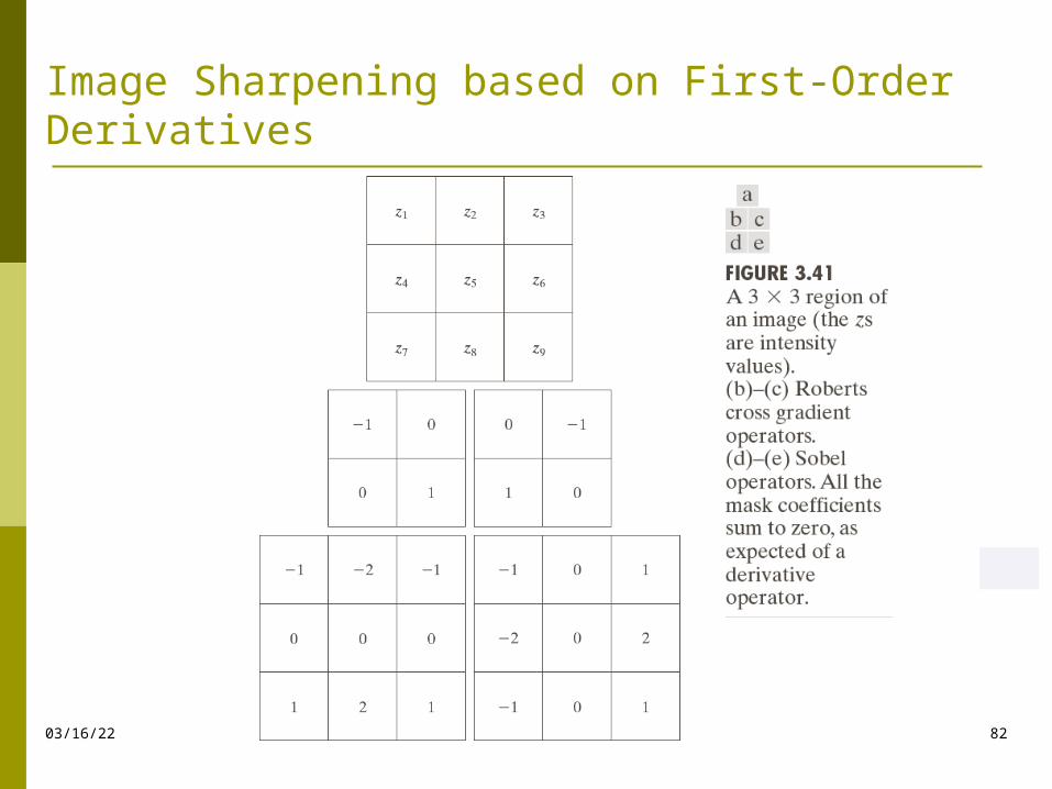
Image Sharpening based on First-Order Derivatives
04/18/23 82

Example
04/18/23 83
04/18/23 84
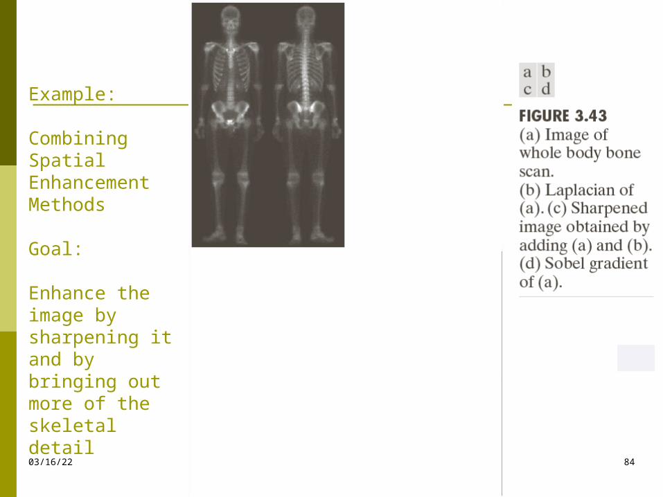
Example:
Combining Spatial Enhancement Methods
Goal:
Enhance the image by sharpening it and by bringing out more of the skeletal detail
04/18/23 85
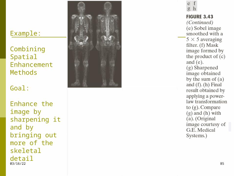
Example:
Combining Spatial Enhancement Methods
Goal:
Enhance the image by sharpening it and by bringing out more of the skeletal detail