cs 514: wavelet analysis of musical...

CS 514: Wavelet Analysis of Musical Signals

Luke Tokheim

http://www.cs.wisc.edu/˜ltokheim/cs514/

May 3, 2002

Contents

1 Input Signals 1

2 Wavelets Used 2

2.1 Daubechies Wavelets . . . . . . . . . . . . . . . . . . . . . . . . . . . . . . . . . . . . 2

2.2 Coiflets . . . . . . . . . . . . . . . . . . . . . . . . . . . . . . . . . . . . . . . . . . . 4

2.3 Biorthogonal Wavelet Systems . . . . . . . . . . . . . . . . . . . . . . . . . . . . . . 4

3 Signal Attack 6

3.1 Introduction . . . . . . . . . . . . . . . . . . . . . . . . . . . . . . . . . . . . . . . . . 6

3.2 Harp Arpeggio . . . . . . . . . . . . . . . . . . . . . . . . . . . . . . . . . . . . . . . 7

4 Frequency Window 13

4.1 Introduction . . . . . . . . . . . . . . . . . . . . . . . . . . . . . . . . . . . . . . . . . 13

4.2 C Major Scale . . . . . . . . . . . . . . . . . . . . . . . . . . . . . . . . . . . . . . . . 13

4.3 Single A440 Note . . . . . . . . . . . . . . . . . . . . . . . . . . . . . . . . . . . . . . 14

5 Conclusions 16

A Matlab Code 17

A.1 Plotting Wavelets . . . . . . . . . . . . . . . . . . . . . . . . . . . . . . . . . . . . . . 17

A.2 Decomposition and Reconstruction . . . . . . . . . . . . . . . . . . . . . . . . . . . . 21

1 Input Signals

Musical signals were chosen for simplicity in feature finding. The simplest signal chosen is a single

tone at a known frequency, particularily A at 440 Hz. It was sampled at 44100 Hz. The second

1

simplest signal is the middle C Major scale. The frequency of each note is known, each note is at

a constant gain, and the notes do not overlap. It was sampled at 22050 Hz. The third simplest

signal chosen is a harp arpeggio, an ascending chord of notes played in fast succession. The signal

covers a wide range of frequency and shows attack and decay features. This signal was sampled at

11025 Hz. A flute music single was also used in one example, it was sampled at 44100 Hz.

2 Wavelets Used

2.1 Daubechies Wavelets

0

Daub 1 (Haar)

0

Daub 4

0

Daub 16

0

Daub 32

Figure 1: Daub1, Daub4, Daub16, Daub32 on time domain.

Daubechies wavelet systems are orthonormal. As the order N of the mother wavelet ψ becomes

larger:

1. support on time domain increases, the interval of support for ψ(t) becomes larger.

2

2. the mother wavelet becomes smoother, more times differentiable. ψ(t) ∈ Cn for some n related

to the order of the wavelet.

3. mother wavelet ψ has more vanishing moments, k. ψ̂(n)(0) = 0, n = 0, . . . , k − 1.

These all lead to better frequency localization. Visually, we can see the size of the interval of

support on the time domain and the improvements in smoothness. But what about the vanishing

moments?

0

1

Daub 1 (Haar), |H0| = 2

−π ≤ ω ≤ π0

1

Daub 4, |H0| = 8

−π ≤ ω ≤ π

0

1

Daub 16, |H0| = 32

−π ≤ ω ≤ π0

1

Daub 32, |H0| = 64

−π ≤ ω ≤ π

Figure 2: Daub1, Daub4, Daub16, Daub32 low-pass filters on frequency domain.

The graphs on the frequency domain of the low-pass filters of the Daubechies wavelet systems

used show a flattening of the function over ω = 0, exactly where we need many derivatives to be 0.

[See figure 2] It would be flat at the origin and at ±π and H0(0) = 1, H0(±π) = 0. As the length

of the low-pass filter H0 increases it becomes closer to the ideal low-pass filter. H0(ω) flattens

about ω = 0 which leads to more 0 derivatives at the origin. Ideally, the filter would be piecewise

constant, H0(ω) = 1 if −π ≤ ω ≤ π and 0 otherwise. [2]

3

For Daubechies wavelet ψ of order N , with |H0| = 2N , the length of the interval of support of

ψ(t) = 2N − 1 and ψ has N vanishing moments. For large N , ψ ∈ CµN , for constant µ ' 0.2. [1]

2.2 Coiflets

Coif 4 Coif 5

Figure 3: Coif4 and Coif5 on time domain.

Coiflet wavelets were also built by Daubechies, and are orthogonal. Coiflets are more symmetri-

cal than Daubechies wavelets. The interval of support of Coiflet ψ of order N is 6N−1, comparable

to Daubchies wavelet of order 3N . ψ of order N has 2N vanishing moments. [1]

0

1

Coif 4

−π ≤ ω ≤ π0

1

Coif 5

−π ≤ ω ≤ π

Figure 4: Coif4 and Coif5 low-pass filters on frequency domain.

2.3 Biorthogonal Wavelet Systems

Biorthogonal wavelet systems use different mother wavelets for decomposition and reconstruction.

This allows the mother wavelets to be symmetric and still have perfect reconstruction. The size

4

Bior 5.5 Deconstruction Bior 5.5 Reconstruction

Bior 6.8 Deconstruction Bior 6.8 Reconstruction

Figure 5: Bior5.5 and Bior6.8 on time domain.

of the support of ψ(t) of order N is 2N − 1. The lengths of the decomposition filters, and the

reconstruction filters can be different and are denoted as BiorR.D, where R is the order of the

reconstruction wavelet and D is the order of the deconstruction wavelet. ψ for decomposition has

N − 1 vanishing moments. [1]

5

0

1

bior 5.5 Deconstruction Filter

−π ≤ ω ≤ π0

1

bior 5.5 Reconstruction Filter

−π ≤ ω ≤ π

0

1

bior 6.8 Deconstruction Filter

−π ≤ ω ≤ π0

1

bior 6.8 Reconstruction Filter

−π ≤ ω ≤ π

Figure 6: Bior5.5 and Bior6.8 low-pass filters on frequency domain.

3 Signal Attack

3.1 Introduction

The attack of a musical signal is a feature that occurs at the beginning of a tone, or note. It is

characterized on the time domain as a sudden increase in the gain of the signal, where gain is the

magnitude of the signal value. The wavelet coefficients represent attack similarily to the signal

on the time domain. A sudden increase in the magnitude of the wavelet coefficients represents an

attack feature in that frequency window of the signal.

While the signal over time only shows that there is attack happening over all frequencies, the

wavelet coefficients also show which frequency windows the attack is active in. In the context of

music, this means that the wavelet coefficients show which pitch range and, equivalently, frequency

ranges are contributing the attack to the musical signal. The fourier transform of the signal also

shows which frequencies are active in the signal. Unfortunately, the fourier transform shows nothing

6

about where in time the frequencies occur. The wavelet coefficients show the signal with respect

to time and frequency. [See figure 7]

Four

ier T

rans

form

of x

(t) o

n fre

quen

cy d

omai

n

Signal x(t) on time domain

Figure 7: An example of attack for a single tone of a flute. The center are the wavelet coefficientsof decomposition with Daubechies with |H0| = 8 for 10 levels. This shows the time-frequencyrepresentation of wavelet analysis.

3.2 Harp Arpeggio

The wavelet decomposition and analysis of the harp arpeggio signal shows the attack and decay

pattern clearly. The attack feature causes a jump in one or for frequency windows and then is

followed by slow decay. As the arpeggio progresses to higher notes, the frequency windows that are

active also also progress to higher frequencies. [See figures 8 through 11]

The Daub1 wavelet system does not show attack features well because the mother wavelet is

not well localized on frequency domain. The attack features shown by the Daub1 system manifest

themselves as smooth bumps with slow increase in magnitude of the wavelet coefficients, or in

7

Partial Reconstruction of signal from wavelet coefficients.At each level, the signal was reconstructed using only wavelet coefficients in that frequency window, all others were zeroed.

Four

ier T

rans

fom

of x

(t) o

n fre

quen

cy d

omai

n


Figure 8: Analysis of arpeggio signal with Daub1. Smooth attack features.

8


Four

ier T

rans

fom

of x

(t) o

n fre

quen

cy d

omai

n


Figure 9: Analysis of arpeggio signal with Daub4. Yields better results than than Daub1, but stillinferior to the other wavelet systems with more vanishing moments.

9


Four

ier T

rans

fom

of x

(t) o

n fre

quen

cy d

omai

n


Figure 10: Analysis of arpeggio signal with Coif5.

10


Four

ier T

rans

fom

of x

(t) o

n fre

quen

cy d

omai

n


Figure 11: Analysis of arpeggio signal with Daub32.

11

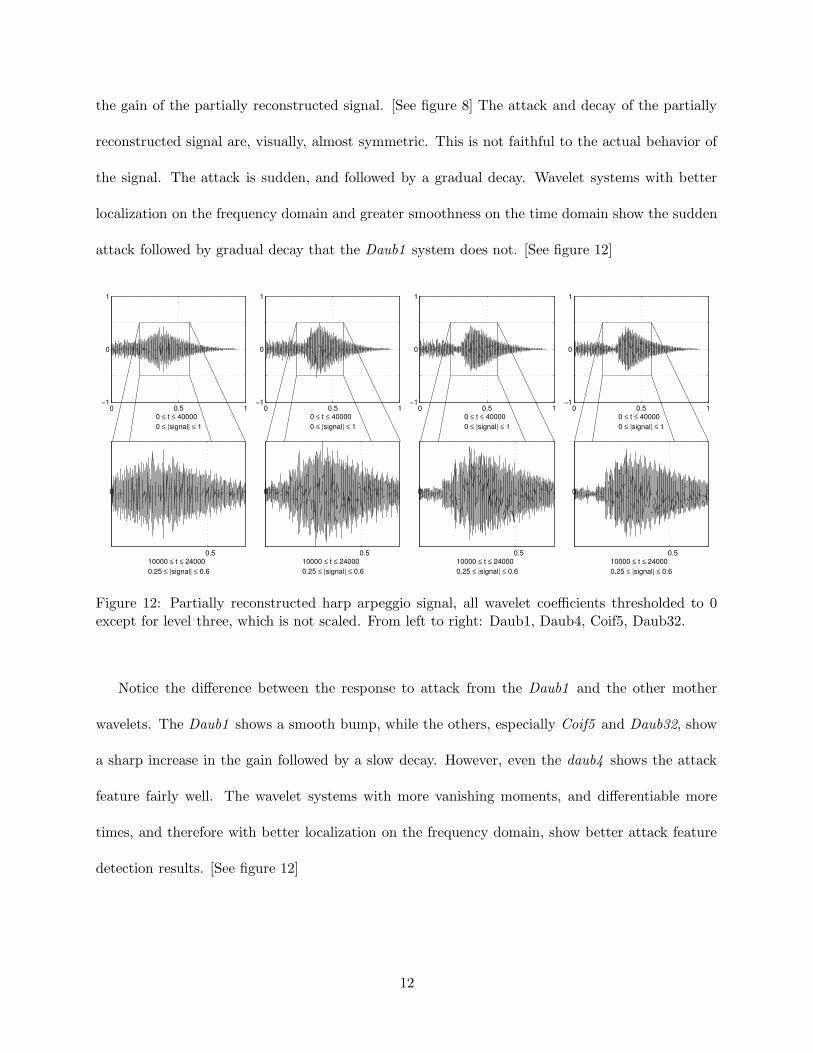
the gain of the partially reconstructed signal. [See figure 8] The attack and decay of the partially

reconstructed signal are, visually, almost symmetric. This is not faithful to the actual behavior of

the signal. The attack is sudden, and followed by a gradual decay. Wavelet systems with better

localization on the frequency domain and greater smoothness on the time domain show the sudden

attack followed by gradual decay that the Daub1 system does not. [See figure 12]

0 0.5 1−1

0

1

0 ≤ t ≤ 400000 ≤ |signal| ≤ 1

0.5

0

10000 ≤ t ≤ 240000.25 ≤ |signal| ≤ 0.6

0 0.5 1−1

0

1

0 ≤ t ≤ 400000 ≤ |signal| ≤ 1

0.5

0

10000 ≤ t ≤ 240000.25 ≤ |signal| ≤ 0.6

0 0.5 1−1

0

1

0 ≤ t ≤ 400000 ≤ |signal| ≤ 1

0.5

0

10000 ≤ t ≤ 240000.25 ≤ |signal| ≤ 0.6

0 0.5 1−1

0

1

0 ≤ t ≤ 400000 ≤ |signal| ≤ 1

0.5

0

10000 ≤ t ≤ 240000.25 ≤ |signal| ≤ 0.6

Figure 12: Partially reconstructed harp arpeggio signal, all wavelet coefficients thresholded to 0except for level three, which is not scaled. From left to right: Daub1, Daub4, Coif5, Daub32.

Notice the difference between the response to attack from the Daub1 and the other mother

wavelets. The Daub1 shows a smooth bump, while the others, especially Coif5 and Daub32, show

a sharp increase in the gain followed by a slow decay. However, even the daub4 shows the attack

feature fairly well. The wavelet systems with more vanishing moments, and differentiable more

times, and therefore with better localization on the frequency domain, show better attack feature

detection results. [See figure 12]

12

4 Frequency Window

4.1 Introduction

The wavelet decompostion of a musical signal shows the amount of activity for the given signal, in

a given frequency range. The musical signal, if viewed on the time domain, only makes the overall

gain of the signal apparent. No judgment can be made about the pitch, or notes that make up

the signal. The fourier tranform of the signal, the representation of the signal on the frequency

domain, would show the amount of a certain frequency present in the signal, but is invariant in

time. There is no way to say that a certain frequency is present at a certain time. However, with

the wavelet decomposition, the amount of a certain level of pitch, or frequency, in a signal at a

given time becomes apparent.

The wavelet decomposition separates the musical signal into pitch or frequency windows. Partial

reconstruction of the signal from only one frequency window shows the signal over time, and limited

to a certain frequency band. By reconstructing for many levels, (I needed at most 10), the musical

signal can be represented in time and frequency simultaneously. This is limited in that the frequency

window is somewhat coarse. For example, the C major scale spans only three frequency windows.

[See figure 13]

4.2 C Major Scale

The eight notes in the C Major scale fall into only three frequency windows. We can draw a

conclusion as to generally what frequency levels are active, such as “The pitches around A440 are

active,” but not exactly which note is active at a given time.

13

t

4

t ω

5

t ω

6

t ω

Original Signal

C D E F G A B C

Wav

elet

Coe

ffici

ents

: Lev

els

4−6

Figure 13: C Major scale. Left: Original musical signal and par-tial reconstruction from one frequency window for three levels.Center: The three frequency windows that contain all pitchesin the scale. Right: The actual frequencies of each note in thescale.

Frequency (Hz ) Note

523.25 C, DO

493.88 B, TI

440.00 A, LA

392.00 G, SO

349.23 F, FA

329.63 E, MI

293.66 D, RE

261.63 C, DO

4.3 Single A440 Note

Partial reconstruction shows which frequency windows are active. Different wavelet systems will

separate the frequency windows more effectively. The wavelet systems with better frequency lo-

calization will not show response in a frequency window that is not actually active. Figure 14

shows ten levels of partial reconstruction from a single level of wavelet decomposition coefficients

of a very simple signal, a digitally generated A440 single tone, with no change in gain. All eight

wavelet systems presented are used to analyse this signal. By looking at the fourier transform of

the signal we can see that all of the signal is at exactly one frequency, and the time domain would

show us the amount of gain over time. The wavelet decomposition and partial reconstruction are

not particularily useful, except to see how the wavelet systems perform with respect to frequency

14

Four

ier T

rans

form

of s

igna

l

Par

tial R

econ

stru

ctio

n of

sig

nal f

rom

wav

elet

coe

ffici

ents

.A

t eac

h le

vel,

all w

avel

et c

oeff.

zer

oed

outs

ide

of c

urre

nt fr

eque

ncy

win

dow

.

Daub 1 Daub 4 Bior 5.5 Bior 6.8 Coif 4 Coif 5 Daub 16 Daub 32

Figure 14: Ten levels of partial reconstruction of A440 note signal ordered by either number ofvanishing moments of mother wavelet ψ or, equivalently, visually.

localization.

We already have a judgement of the frequncy localization in the number of vanishing moments

of the wavelets. Figure 14 orders the wavelet analyses from left to right by increasing vanishing

moments and support on time domain. The results confirm that the performance of the wavelets

are ordered as expected.

The results of partial reconstruction differs substantially between the chosen wavelet systems.

The wavelet systems with less vanishing moments show response in frequency windows that should

not. This is because the wavelet system is not local enough in frequency. The wavelet system

15

is spreading frequency information between the frequency windows. As the number of vanishing

moments of the wavelet system increases, the quality of the partial reconstruction improves. [See

figure 14] The table of partial reconstructions is ordered by number of vanishing moments of mother

wavelet ψ, but it is also ordered as quality of results. They imply each other.

5 Conclusions

Wavelet analysis of musical signals is useful to show features in both time and frequency simul-

taneously. This is advantageous because the benefits of both domains can be taken advantage of.

Having only access to the signal on the time domain and the fourier transform of that signal on

the frequency domain is not very useful unless there is a way to relate them.

The time-frequency representation of the signal shows the signal as neither time nor frequency

could show independently. The frequency windows allow the independent analysis of a particular

frequency range with respect to time. Without the time-frequency representation we could not

draw a conclusion like, “There was an attack at time t in frequency range [a, b].” Whether or not

this is useful for actual applications is unclear. The application must take advantage of the ability

to look time and frequency simultaneously to reap the benefits of wavelet signal analysis.

References

[1] Matlab. Online help and command waveinfo. Matlab refers to I. Daubechies.

[2] Ron, Amos. CS 514 online lecture notes (2002).

16

A Matlab Code

A.1 Plotting Wavelets

biorPlot.m

function biorPlot

clf;

[y dy] = plotBiorWavelet(10,’bior5.5’);

subplot(2,2,1); plot(y);

axis([2000 8000 -.0004 .0016])

title(’Bior 5.5 Deconstruction’);

set(gca,’ytick’,0,’xtick’,0,’yticklabel’,’’,’xticklabel’,’’);

subplot(2,2,2); plot(dy);

axis([1500 8500 -.0001 .0009]);

title(’Bior 5.5 Reconstruction’);


[y dy] = plotBiorWavelet(10,’bior6.8’);

subplot(2,2,3); plot(y);

axis([1500 8500 -.0002 .0011])

title(’Bior 6.8 Deconstruction’);


subplot(2,2,4); plot(dy);

axis([4000 12000 -.0002 .0013])

title(’Bior 6.8 Reconstruction’);


coifPlot.m

function coifPlot

clf;

y = plotCoifWavelet(10,’coif4’);

subplot(2,2,1); plot(y); axis([3000 17000 -.0002 .0012])

title(’Coif 4’);


y = plotCoifWavelet(10,’coif5’);

subplot(2,2,2); plot(y); axis([3000 17000 -.0002 .0012])



daubPlot.m

17

function daubPlot

clf;

y = plotDaubWavelet(10,’db1’);

subplot(2,2,1); plot(y); axis([0 2000 -0.0001 .0011]);

title(’Daub 1 (Haar)’);

set(gca,’ytick’,[0 2000],’xtick’,0,’yticklabel’,[0 2000],’xticklabel’,’’);


subplot(2,2,2); plot(y); axis([0 6000 -.0004 .00125]);

title(’Daub 4’);










graphBiorHs.m

function graphBiorHs

clf;

x = linspace(-pi,pi,512);

[h rh] = biorwavf(’bior5.5’);

h = fftshift(fft(h,512));

subplot(2,2,1);

plot(x,abs(h));

title(’bior 5.5 Deconstruction Filter’);

axis([-pi pi 0 1.3]);

set(gca,’ytick’,[0 1],’xtick’,0,’yticklabel’,[0 1],’xticklabel’,’’)

set(gca,’ygrid’,’on’,’xgrid’,’on’);

xlabel(’-\pi \leq \omega \leq \pi’);

rh = fftshift(fft(rh,512));

subplot(2,2,2);

plot(x,abs(rh));

title(’bior 5.5 Reconstruction Filter’);

axis([-pi pi 0 1.3]);



18


[h rh] = biorwavf(’bior6.8’);

h = fftshift(fft(h,512));

subplot(2,2,3);

plot(x,abs(h));

title(’bior 6.8 Deconstruction Filter’);

axis([-pi pi 0 1.3]);




rh = fftshift(fft(rh,512));

subplot(2,2,4);

plot(x,abs(rh));

title(’bior 6.8 Reconstruction Filter’);

axis([-pi pi 0 1.3]);




graphCoifHs.m

function graphCoifs

clf


h = coifwavf(’coif4’); h = fftshift(fft(h,512));

subplot(2,2,1);

plot(x,abs(h));


axis([-pi pi 0 1.1]);


set(gca,’xgrid’,’on’,’ygrid’,’on’);


h = coifwavf(’coif5’); h = fftshift(fft(h,512));

subplot(2,2,2);

plot(x,abs(h));


axis([-pi pi 0 1.1]);




graphDaubHs.m

19

function graphDaubHs

clf


h = dbwavf(’db1’); h = fftshift(fft(h,512));

subplot(2,2,1); plot(x,abs(h));

title(’Daub 1 (Haar), |H_{0}| = 2’);

axis([-pi pi 0 1.1]);






title(’Daub 4, |H_{0}| = 8’);

axis([-pi pi 0 1.1]);






title(’Daub 16, |H_{0}| = 32’);

axis([-pi pi 0 1.1]);






title(’Daub 32, |H_{0}| = 64’);

axis([-pi pi 0 1.1]);




plotBiorWavelet.m

function [y,dy] = plotBiorWavelet(iterations, name)

% plot a bior wavelet on time domain

y = [1 0];

dy = [1 0];

[h dh] = biorwavf(name);

for i=1:iterations,

y = upsample(y);

20

dy = upsample(dy);

y = conv(h, y);

dy = conv(dh, dy);

end

plotCoifWavelet.m

function y = plotCoifWavelet(iterations, name)

% plot a coiflet on time domain

y = [1 0];

h = coifwavf(name);

for i=1:iterations,

y = upsample(y);

y = conv(h, y);

end

plotDaubWavelet.m

function y = plotDaubWavelet(iterations, name)

% plot a daub wavelet on time domain

y = [1 0 0];

h = dbwavf(name);

for i=1:iterations,

y = upsample(y);

y = conv(h, y);

end

upsample.m

function y = upsample(x)

for i=1:length(x),

y(2*i-1) = x(i);

end

A.2 Decomposition and Reconstruction

graphAttack.m

function graphAttack(x,wname)

% plot a detail of signal with an attack feature

clf;

n = 8;

21

for i=1:n,

[y detail] = partialRec(x,i,wname);

subplot(n, 2, (2*i));

plot(detail);

axis([(length(detail)/5) (length(detail)/2) -1 1]);

set(gca,’ytick’,0,’xtick’,0,’yticklabel’,i,’xticklabel’,’’);

end

graphPartialRec.m

function graphPartialRec(x,n,wname)

% plot a table of n partial reconstructions

clf;

n = (n+1);

h = subplot(n, 2, 1);

plot(x); axis([0 length(x) -1 1]);


for i=2:n,

[y detail] = partialRec(x,(i-1),wname);

subplot(n, 2, (2*i-1));

plot(y);

axis([0 length(y) -1 1]);



plot(detail);

axis([0 length(detail) -1 1]);


end

graphPartialRecAllWavelets.m

function graphPartialRecAllWavelets(x,n,m,wname)

% plot a table of n partial reconstructions

% at column m

num = 1; % number wavelet systems

for i=1:n,

[y detail] = partialRec(x,i,wname);

subplot(n, num, (num*(i-1)+m));

plot(y);



end

22

graphPartialRecRange.m

function graphPartialRecRange(x,start,n,wname)

% plot a range of n partial reconstructions

% starting at index start

clf;

n = (n+1);

h = subplot(n, 2, 1);

plot(x); axis([0 length(x) -1 1]);

xlabel(’t’);


for i=2:n,

[y detail] = partialRec(x,(i-1+start),wname);

subplot(n, 2, (2*i-1));

plot(y); xlabel(’t’);


set(gca,’ytick’,0,’xtick’,0,’yticklabel’,(i-1+start),’xticklabel’,’’);


plot(detail); xlabel(’\omega’);

axis([0 length(detail) -1 1]);


end

partialRec.m

function [y, detail] = partialRec(x, level, name)

% signal [y, detail] = partialRec(signal x, int level, string waveletname)

% do deconstruction with specified wavelets to level ’level’, and then do

% partial reconstruction, zeroing all levels > ’level’

%

% code based on Assignment 5 solution

cD = cell(level,1);

cA = x;

for i=1:level,

[cA cD{i}] = dwt(cA, name);

end

detail = cD{level};

cA = zeros(length(cD{level}), 1);

cA = idwt(cA, cD{level}, name);

23

for i=(level-1):-1:1,

cA = cA([1:length(cD{i})]);

cA = idwt(cA, zeros(length(cD{i}), 1), name);

end

y = cA;

24

cs 514: wavelet analysis of musical...

Documents