cs 376 computer graphics - skidmore collegemeckmann/2014spring/cs325/s2014_01_29.pdfmichael eckmann...

CS 325Introduction to Computer Graphics

01 / 29 / 2014

Instructor: Michael Eckmann

Michael Eckmann - Skidmore College - CS 325 - Spring 2014

Today’s Topics• Comments/Questions?• Bresenham-Line drawing algorithm• Midpoint-circle drawing algorithm• Ellipse drawing• Antialiasing• Polygons• Polygon filling algorithm


Bresenham's Line Algorithm• Bresenham's Algorithm is efficient (fast) and accurate.• The key part of Bresenham's algorithm lies in the determination

of which pixel to turn on based on whether the line equation would cause the line to lie more near one pixel or the other.


Bresenham's Line Algorithm• Think of a line whose slope is >0, but < 1. These are first octant lines (the

area of the coordinate plane between the positive x-axis and the line y=x.)

• Assume we have the pixel at (xk, yk) turned on and we're trying to determine between the following:

– Should (xk+1, yk) or (xk+1, yk+1) be on?

– That is, the choice is between either the pixel one to the right of (xk, yk)

or the pixel one to the right and one up.

• The decision can be made based on whether dlower - dupper is positive or not.

• The goal is to come up with an inexpensive way to determine the sign of

(dlower – dupper )


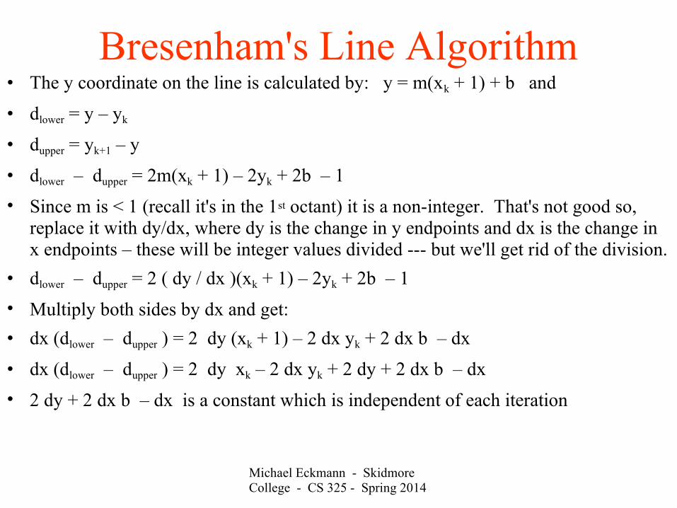
Bresenham's Line Algorithm• The y coordinate on the line is calculated by: y = m(xk + 1) + b and

• dlower = y – yk

• dupper = yk+1 – y

• dlower – dupper = 2m(xk + 1) – 2yk + 2b – 1

• Since m is < 1 (recall it's in the 1st octant) it is a non-integer. That's not good so, replace it with dy/dx, where dy is the change in y endpoints and dx is the change in x endpoints – these will be integer values divided --- but we'll get rid of the division.

• dlower – dupper = 2 ( dy / dx )(xk + 1) – 2yk + 2b – 1

• Multiply both sides by dx and get:

• dx (dlower – dupper ) = 2 dy (xk + 1) – 2 dx yk + 2 dx b – dx

• dx (dlower – dupper ) = 2 dy xk – 2 dx yk + 2 dy + 2 dx b – dx

• 2 dy + 2 dx b – dx is a constant which is independent of each iteration


Bresenham's Line Algorithm• So we end up with

• dx (dlower – dupper ) = 2 dy xk – 2 dx yk + c

• We only need to determine the sign of (dlower – dupper )

• dx is positive so it doesn't have an effect on the sign (so now there's no need to divide) --- does that make sense?

• Let pk = dx (dlower – dupper ) pk is the decision parameter

• So, we check if 2 dy xk – 2 dx yk + c < 0 and if it is we turn on the lower pixel, so

(xk+1, yk) should be the pixel turned on

• otherwise (xk+1, yk+1) is turned on

• As the algorithm iterates though it needs to then calculate the next value of p, which

is pk+1


Bresenham's Line Algorithm• Recall that to calculate pk we had: pk = 2 dy xk – 2 dx yk + c

• So, pk+1 = 2 dy xk+1 – 2 dx yk+1 + c

• If we subtract pk+1 – pk = 2dy ( xk+1 – xk ) – 2dx ( yk+1 – yk )

• But, xk+1= xk + 1 because the first octant slope always increment x by 1

• So, we have pk+1 – pk = 2dy – 2dx ( yk+1 – yk )

• Then, pk+1 = pk + 2dy – 2dx ( yk+1 – yk )

• Where ( yk+1 – yk ) is either 1 or 0 (why?) depending on the sign of pk . So, either

• pk+1 = pk + 2dy (when pk < 0)

• pk+1 = pk + 2dy – 2dx (when pk >= 0)


Initial decision variable value• The initial value of p in the Bresenham line algorithm

is calculated by using the equation for p with (x0, y0)• Derivation:

pk = 2dyxk – 2dxyk + cwhere c = 2dy + dx(2b-1)and since yk=mxk+b, b = yk–mxk and m = dy/dx

pk = 2dyxk – 2dxyk + 2dy + dx(2(yk– (dy/dx)xk)– 1)multiplied out:pk = 2dyxk – 2dxyk + 2dy + 2dxyk– 2dyxk – dx = 2dy – dx


Bresenham's Line Algorithm/* Bresenham line-drawing procedure for |m| < 1.0. */

void lineBres (int x0, int y0, int xEnd, int yEnd)

{

int dx = fabs (xEnd - x0), dy = fabs(yEnd - y0);

int p = 2 * dy - dx;

int twoDy = 2 * dy, twoDyMinusDx = 2 * (dy - dx);

int x, y;

/* Determine which endpoint to use as start position. */

if (x0 > xEnd) {

x = xEnd;

y = yEnd;

xEnd = x0;

}

else {

x = x0;

y = y0;

}

setPixel (x, y);

while (x < xEnd) {

x++;

if (p < 0)

p += twoDy;

else {

y++;

p += twoDyMinusDx;

}

setPixel (x, y);

}

}

/* From Hearn & Baker's Computer Graphics with OpenGL, 3rd Edition */


Circle Algorithms


Circle Algorithms• So, we only need to calculate the coordinates of an eighth of the circle and plot the

following:

• (-x, -y), (-x, y), (x, -y), (x, y), (y, x), (y, -x), (-y, x), (-y, -x)

• Bresenham's Line Algorithm has been adapted to circles by deciding which pixel is closest to the actual circle at each sampling step.

• It should be able to draw circles with any center, but to make calculations easier, compute the pixel coordinates based on the same radius but centered at the origin. Then when you plot the pixel, add in the center coordinates.

• Consider only the octant between the lines x=0 and y=x. The slope of the curve varies from 0 (at the top) to -1 at the 45 degree angle. This implies that we should do unit steps on the x-axis and calculate y (I leave this for you to convince yourself that this is the right approach.)

• At each x, the decision is between which y is correct among two possible y's, the one to the right or the one to the right and down.


Circle Algorithms


Circle Algorithms• The decision is always between the pixel one to the right or one to the right and one

down. Respectively, yk or yk -1.

• The midpoint circle algorithm is a way to determine it using only integer arithmetic.

• Define a circle function as f(x,y) = x2 + y2 – r2

• A point x,y on the circle with radius r will cause f(x,y) = 0

• A point x,y in the circle's interior will cause f(x,y) < 0.

• A point x,y outside the circle will cause f(x,y) > 0.

• The point we use is the midpoint between the two pixel choices. And f(x,y) as defined above is our decision variable pk

• The point is (xk + 1, yk – ½)

• If pk is < 0, it is inside the circle and closer to yk

• Otherwise choose yk -1


Circle Algorithms• pk = f(xk + 1, yk – ½) = (xk + 1)2 + (yk – ½)2 – r2

• If pk is < 0, it is inside the circle and closer to yk

• Otherwise choose yk -1

• pk+1 = f(xk+1 + 1, yk+1 – ½) = (xk+1 + 1)2 + (yk+1 – ½)2 – r2

• pk+1 = ((xk + 1) + 1)2 + (yk+1 – ½)2 – r2 (pk+1can be expressed in terms of pk )

• Similar to how we determined the recursive decision variable computation in Bresenham's Line Algorithm, we do for the Circle Algorithm as well: skipping a bunch of steps leads to:

• pk+1 = pk + 2xk+1 + 1 (when pk < 0)

• pk+1 = pk + 2xk+1 + 1 – 2yk+1 (otherwise)

• Assuming we start at point (0,r), we'll have p0 = f(0 + 1, r – ½) = f(1, r – ½) which yields

5/4 – r (or 1– r for integer radii because of rounding)

• Let's plot some points as an example for a circle of radius 6, and center (-2, 4)

• We do calculations with center 0,0 and for each point we plot, we add in the center.


Circle Algorithm Example

Center = (-2, 4)

K

0 -5 (1, 6) (-1, 10) 2 12

1 -2 (2, 6) (0, 10) 4 12

2 3 (3, 5) (1, 9) 6 10

Pk

(xk+1

, yk+1

) Center + (xk+1

, yk+1

) 2xk+1

2yk+1

• p0 = 1– r

• pk+1 = pk + 2xk+1 + 1 (when pk < 0)

• pk+1 = pk + 2xk+1 + 1 – 2yk+1 (otherwise)

• Plot: (-1, 10), (0, 10), (1, 9), (2, 8)

• Also, plot points in the other 7 octants for each of these four.

• e.g. The other 7 points for (-1, 10) to plot are:

•(-3, 10), (-1,-2), (-3,-2), (4,5), (4, 3), (-8, 5), (-8, 3)

•These were calculated by adding the center (-2,4) to (-1,6), (1,-6), (-1,-6), (6, 1), (6,-1), (-6,1), and (-6,-1)


Circle Algorithms• There's a figure in the text book (figure 6-15) and it looks to me like the circle line is

drawn incorrectly but the pixels are correct. It is showing the center of the circle at the bottom left corner of the 0,0 pixel box, but it should be in the center of the 0,0 pixel box.

• I noticed it because when x=3, based on the drawn circle, the algorithm would “turn on” (3,9) not (3,10), because the midpoint is clearly outside the circle there.

• I didn't verify it, but I trust the calculations in the table which says that p2 = -1 which would be inside the circle.


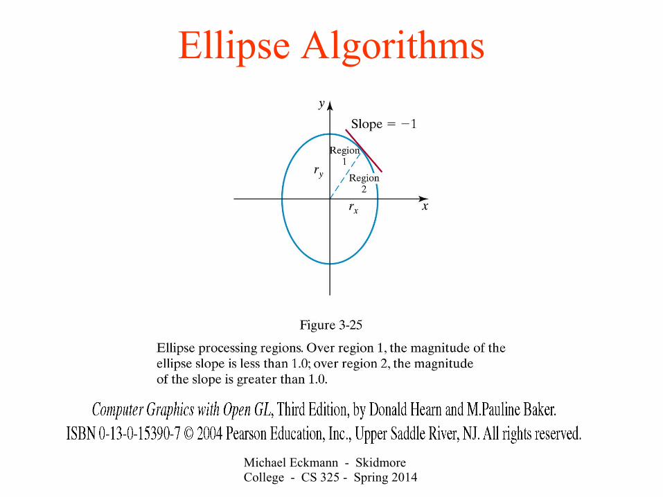
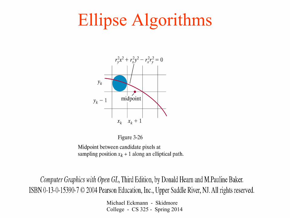
Ellipse Algorithm• We can generalize the circle algorithm to generate ellipses but

with only 4-way symmetry.

• The slope of the ellipse changes from > -1 to < -1 in one quadrant so that we will have to switch from – unit samples along the x-axis and calculate y– to unit samples along the y-axis and calculate x

• I'm not as concerned about the details of ellipses as I am with

you understanding the details of the line and circle algorithms.


Ellipse Algorithms


Antialiasing

• Aliasing is the distortion we see when we undersample. The

jaggedness stairstep quality of lines is an example of aliasing.

• Solutions:– Higher addressability

• e.g. Move from a 800x600 grid to a 1280x1024 grid and your lines will look smoother.

• If keep addressability fixed then we can change the intensity of the pixels being turned on. Instead of turning on one pixel at full intensity, we appropriately weight the intensities of two pixels at each step to cause the illusion of a point living at some intermediate location between the two pixel centers.


Antialiasing

• Example on the board.


Antialiasing

• Any ideas on how we could adapt Bresenham's line algorithm to

do antialiased lines?


Antialiasing

• Any ideas on how we could adapt Bresenham's line algorithm to

do antialiased lines?

• dlower + dupper = 1

• The upper pixel's intensity

can be set to be dlower

• The lower pixel's intensity

can be set to be dupper

• When the line passes exactly through the center of a pixel, that

pixel's intensity is 1 and the other is 0 (off).


Antialiasing• Supersampling is a technique to treat the screen as a finer grid than is

actually addressable and plot the points by turning on multiple points in

the finer grid. Then when ready to display --- use the finer grid points to

determine the intensities of the pixels of the actual screen.

• Example --- divide each actual addressable pixel into 9 (3x3) finer

subpixels. Draw a Bresenham line on the subpixels. Then base the

intensity of actual pixel on how many of the 9 subpixels would be on. – 3 subpixels is max, so that's full intensity– 2 subpixels could cause the pixel to be at 2/3 intensity– 1 subpixel on could cause the pixel to be at 1/3 intensity– 0 would be off


Antialiasing

• Alternately, we could use a weighting mask that would give more

weight to the center subpixel of the 3x3 grid1 2 1

2 4 2

1 2 1

• Another alternative is to treat the line as a rectangle of width 1

pixel & draw it on the finer grid (w/ 9 subpixels per pixel). Then

how many of the 9 subpixels are on (on = bottom left corner of

subpixel is inside the rectangle) determines the intensity of pixel

(9 = full intensity, 8 = 8/9 intensity, etc.) This is better than the

three intensity levels of the other supersampling method.


Antialiasing• Area sampling is a technique that computes areas of overlap of

each pixel with the object (e.g. line or polygon) to be displayed.

• This is similar to the supersampling method described last

(treating the line as a rectangle), but instead of just 9 different

intensities, let the intensity of a pixel be the area of the rectangle

that overlaps the pixel / the area of the whole pixel.


Antialiasing• There are other techniques to do antialiasing --- filtering

techniques. These are similar to the discrete mask two slides ago,

except they work with a continuous function to determine the

weightings of the pixels. Examples on the next slide show a box, a

cone and a gaussian. The volumes of these are normalized to 1

and to determine the weighting of a pixel we integrate the function

over the pixel surface. Since integrating is expensive (in time)

lookup tables can be used.


Antialiasing


Antialiasing also helps with ...• Notice: without antialiasing, compare a line with slope = 1 made

up of n pixels and a line with slope = 0 made up of n pixels.

• The slope = 1 line is SQRT(2) longer but is made up of the same

number of pixels. What do you think is the visual effect of this?


Antialiasing helps total intensity• See figures 6-63 & 6-64 in text.

• In addition to lines looking straighter, when using the antialiasing

technique that treats lines as having some finite width, lines of

different angles will not have different total intensities.


Polygons• 3 or more vertices describe a polygon. The vertices are

connected with line segments (called an edge, or a side). Each

edge can only have endpoints in common with any other edge.

• Definition of convex polygon – Def 1: All interior angles are < 180 degrees– Def 2: The interior lies completely on 1 side of the infinite

extension of any edge.– Def 3: If we select any two interior points, the line segment

joining them is also fully in the interior of the polygon

• Definition of concave polygon– Not convex.


Polygons• Degenerate polygons are

– Those with 3 or more collinear vertices– Those with repeated vertices– Etc.


Polygon interior points• A common operation is to determine if a point is in the interior of

a polygon or not.

• One way to do it is, for some point, draw a horizontal line from

that point to a distant point outside the possible area of the

polygon and count how many times the horizontal line crosses

edges of the polygon.

• If the line crosses an odd number of edges, then it is an interior

point. If it crosses an even number of edges, then it is exterior.

• Example on board.


Polygon interior points• What happens when the horizontal line crosses a vertex. Should it

be counted as 1 or 2?



Polygon interior points• What happens when the horizontal line crosses a vertex. Should it

be counted as 1 or 2?

• If the vertex is a local maximum or a local minimum then count it

as 2. Otherwise count it as 1.


Polygon fill areas• Polygons in OpenGL are specified by vertices. It is good to get

into the habit now that you specify the vertices in

counterclockwise order.

• The reason for this is, when we do some things later this semester

like displaying 3D objects, we're going to care about which side

(face) of the polygon is visible.

• The front face of a polygon is visible when its vertices are in

counterclockwise order. We'll know if we're seeing the back face

of a polygon if they are in clockwise order.


Polygon fill areas• To do a scanline fill of a polygon (see figure 6-46, 47, 48).

– Determine the intersections (crossings) of the horizontal line (y=c) with the edges (y=mx + b) of the polygon.

– Sort the crossings (x coordinates) from low to high (left to right).

– There will be an even number of crossings, so draw horizontal lines between the first two crossings, then the next 2 and so on.

– If the scanline goes through a vertex• Add the crossing to the list twice if it's a local max or min.• Add the crossing only once otherwise.

• Horizontal edges of a polygon can be ignored (not turned on.)



Polygon fill areas• Another way to determine how many to count if the scanline goes

through a vertex• If the two edges are on the same side of the scanline, then

add it twice.• If the two edges are on different sides of the scanline, then

add it once.

• To check for this, we can compare the y coordinates of the 3

vertices in question (draw on board) in either clockwise or

counterclockwise fashion– If all 3 are monotonically increasing or all 3 are monotonically

decreasing then the two edges are on different sides.


Polygon fill areas• Edge coherence properties can be used to speed up the calculation of the

crossings of the scanline and edges. The crossing x-coordinate of one

scanline with an edge differs from the crossing of the x-coordinate of the

next scanline only by 1/m as seen below.

• Assuming we're processing the fill from bottom to top and the y's

increase as we go up, – Assume scan line yk crosses an edge at (xk , yk ) and yk+1 crosses at

(xk+1, yk+1)

– m = (yk+1 – yk) / (xk+1 – xk )

– (yk+1 – yk) = 1, so, m = 1 / (xk+1 – xk ) and solve for xk+1

– So, scan line yk+1 crosses that edge at (xk + 1/m, yk+1 )• This is less processing than doing the intersection of y = yk+1 with

y = mx + b which is x = (yk+1+b)/m.


Polygon fill areas• Efficient polygon filling

– 1) proceed around edges in a clockwise or counterclockwise fashion– 2) store each edge in an edge table– 3) sort the edges based on the minimum y in the edge– 4) process the scanlines in a bottom to top order– 5) when the current scanline reaches the lower endpoint (with the

min y) of the edge, that edge becomes active– 6) active edges are sorted by their x coordinates (left to right)– During any given scanline non-active edges can be marked as either

finished, or not yet active. Horizontal edges are ignored.



Polygon fill areas• Masks

– Besides being filled with a solid color, polygons are sometimes filled with patterns. The process of filling an area with a pattern is called tiling.

– Fill patterns can be stored as rectangular arrays. The arrays are called masks and they are applied to the fill area and are usually smaller than the area to be filled.

– The mask needs a starting position within the area to be filled. Starting at this position the mask is replicated both vertically and horizontally.

– If the mask is an m × n array, and starting position is (0,0) a pixel at (x, y) will be drawn with the color in mask((x mod n), (y mod m)).

– Example on board.


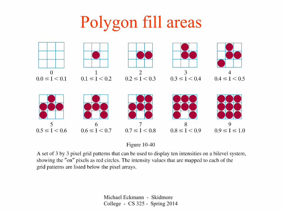
Polygon fill areas• Section 17.9 Halftoning and dithering

– When there are very few intensity levels available (e.g. 2, black & white) to be displayed, halftoning is a technique that can provide more intensities with the tradeoff in addressability.

– Newspapers show grey level photos by displaying black circles. The black circles vary in size according to how dark that part of the photo should be.

– In graphics systems this halftoning technique is approximated with halftone patterns. Halftone patterns are typically n × n squares of pixels where the number of pixels turned on in that pattern correspond to the intensity desired.


Polygon fill areas• How is halftoning a tradeoff between intensities and addressability

(resolution) ?


Polygon fill areas• Guidelines to creating halftoning patterns

– With halftoning, one thing to be careful about is that unintended patterns can become apparent. The intent is to have the viewer see the increase in intensities without noticing unintentional patterns.

– Avoid only horizontal or vertical or diagonal pixels on in the patterns to reduce the possibility of “streaks”.

– Further it is good to approximate the way that newspapers do it --- that is, concentrate on turning on pixels in the center of the pattern at each successive intensity.

– To minimize unintentional patterns to be displayed, we can evolve each successive grid pattern by copying it and turning on an additional pixel.

• See next slide figure 10-40.


Polygon fill areas


Polygon fill areas• Dithering

– Dithering refers to techniques for approximating halftones but without reducing addressability (resolution).

– An n×n dither matrix Dn is used to detemine if a pixel should be on or off.

– The matrix is filled with the numbers from 0 to n2 – 1– on page 534 (equation 17-49) there's a mistake, it should be the

dither matrix D4

15 7 13 5 3 11 1 912 4 14 6 0 8 2 10


Polygon fill areas• Example of dither matrix D4

15 7 13 5 3 11 1 912 4 14 6 0 8 2 10

– For some pixel (x, y) an intensity level I(x,y) between 0 and n2 is desired. Compute i = x mod n and j = y mod n to find which element (i,j) of the matrix Dn to compare to the desired intensity.

– If I(x,y) > Dn(i,j) then the pixel is turned on, otherwise it is not.– This has the effect of different intensities, without reducing

resolution. But what gets lost?

cs 376 computer graphics - skidmore collegemeckmann/2014spring/cs325/s2014_01_29.pdfmichael eckmann...

Documents