CS 345:Topics in Data Warehousing

Thursday, October 7, 2004

Review of Thursday’s Class• 4-step dimensional modeling process

– Decide which process to model– Choose the grain for the fact table– Select the dimensions– Select the numeric measures for the facts

• Dimension topics– Date dimension– Surrogate keys– Degenerate dimensions– Snowflakes

• Fact topics– Additivity– Transactional vs. Snapshot

Outline of Today’s Class

• Facts– Semi-additive facts– “Factless” fact tables

• Slowly Changing Dimensions– Overwrite history– Preserve history– Hybrid schemes

• More dimension topics– Dimension roles– Junk dimension

• More fact topics– Multiple currencies– Master/Detail facts and fact allocation– Accumulating Snapshot fact tables

Transactional vs. Snapshot Facts

• Transactional– Each fact row represents a discrete event– Provides the most granular, detailed information

• Snapshot– Each fact row represents a point-in-time snapshot– Snapshots are taken at predefined time intervals

• Examples: Hourly, daily, or weekly snapshots

– Provides a cumulative view– Used for continuous processes / measures of intensity– Examples:

• Account balance• Inventory level• Room temperature

Transactional vs. Snapshot Facts

Brian Oct. 1 CREDIT +40

Rajeev Oct. 1 CREDIT +10

Brian Oct. 3 DEBIT -10

Rajeev Oct. 3 CREDIT +20

Brian Oct. 4 DEBIT -5

Brian Oct. 4 CREDIT +15

Rajeev Oct. 4 CREDIT +50

Brian Oct. 5 DEBIT -20

Rajeev Oct. 5 DEBIT -10

Rajeev Oct. 5 DEBIT -15

Brian Oct. 1 40

Rajeev Oct. 1 10

Brian Oct. 2 40

Rajeev Oct. 2 10

Brian Oct. 3 30

Rajeev Oct. 3 30

Brian Oct. 4 40

Rajeev Oct. 4 80

Brian Oct. 5 40

Rajeev Oct. 5 55

Transactional Snapshot

Transactional vs. Snapshot Facts

• Two complementary organizations• Information content is similar

– Snapshot view can be always derived from transactional fact– But not the other way around.

• Why use snapshot facts?– Sampling is the only option for continuous processes

• E.g. sensor readings

– Data compression• Recording all transactional activity may be too much data!• Stock price at each trade vs. opening / closing price

– Query expressiveness• Some queries are much easier to ask/answer with snapshot fact• Example: Average daily balance

Semi-Additive Facts

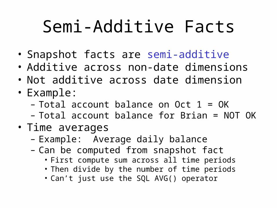
• Snapshot facts are semi-additive• Additive across non-date dimensions• Not additive across date dimension• Example:

– Total account balance on Oct 1 = OK– Total account balance for Brian = NOT OK

• Time averages– Example: Average daily balance– Can be computed from snapshot fact

• First compute sum across all time periods• Then divide by the number of time periods• Can’t just use the SQL AVG() operator

Factless Fact Tables• Transactional fact tables don’t have rows for non-events

– Example: No rows for products that didn’t sell• This has good and bad points.

– Good: Take advantage of sparsity• Much less data to store if events are “rare”

– Bad: No record of non-events• Example: What products on promotion didn’t sell?

• “Factless” fact table– A fact table without numeric fact columns– Used to capture relationships between dimensions– Include a dummy fact column that always has value 1

• Examples:– Promotion coverage fact table

• Which products were on promotion in which stores for which days?• Sort of like a periodic snapshot fact

– Student/department mapping fact table• What is the major field of study for each student?• Even for students who didn’t enroll in any courses…

Slowly Changing Dimensions

• Compared to fact tables, contents of dimension tables are relatively stable.– New sales transactions occur constantly.– New products are introduced rarely.– New stores are opened very rarely.

• Attribute values for existing dimension rows do occasionally change over time– Customer moves to a new address– Grouping of stores into districts, regions changes due to

corporate re-org

• How to handle gradual changes to dimensions?– Option 1: Overwrite history– Option 2: Preserve history

Overwriting History

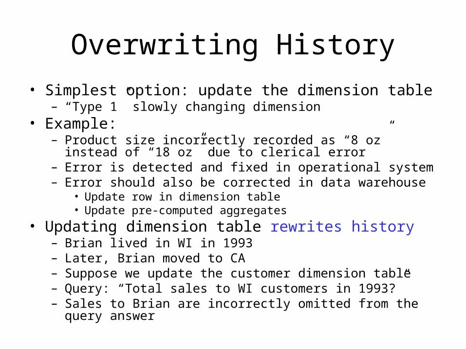
• Simplest option: update the dimension table– “Type 1” slowly changing dimension

• Example: – Product size incorrectly recorded as “8 oz” instead of “18 oz”

due to clerical error– Error is detected and fixed in operational system– Error should also be corrected in data warehouse

• Update row in dimension table• Update pre-computed aggregates

• Updating dimension table rewrites history– Brian lived in WI in 1993– Later, Brian moved to CA– Suppose we update the customer dimension table– Query: “Total sales to WI customers in 1993?”– Sales to Brian are incorrectly omitted from the query answer

Preserving History

• Accurate historical reporting is usually important in a data warehouse

• How can we capture changes while preserving history?• Answer: Create a new dimension row

– Old fact table rows point to the old row– New fact table rows point to the new row– “Type 2” slowly changing dimension

Cust_key Name Sex State YOB

457 Brian Male WI 1976

… … … … …

784 Brian Male CA 1976

Customer Dimension

Old dimension row

New dimension row

Slowly Changing Dim. Example

Cust_key Name Sex State YOB

457 Brian Male WI 1976

… … … … …

784 Brian Male CA 1976

Customer Dimension

Cust_key … Quantity

… … …

457 … 5

… … …

784 … 4

Sales Fact

Existing fact rows use old dimension row

New fact rows use new dimension row

Pros and Cons

• Type 1: Overwrite existing value+ Simple to implement

• Type 2: Add a new dimension row+ Accurate historical reporting+ Pre-computed aggregates unaffected- Dimension table grows over time

• Type 2 SCD requires surrogate keys– Store mapping from operational key to most current surrogate

key in data staging area

• To report on Brian’s activity over time, constrain on natural key – WHERE name = ‘Brian’

Choosing Type 1 vs. Type 2

• Both choices are commonly used• Easy to “mix and match”

– Preserve history for some attributes– Overwrite history for other attributes

• Questions to ask:– Will queries want to use the original attribute value or

the new attribute value?• In most cases preserving history is desirable

– Does the performance impact of additional dimension rows outweigh the benefit of preserving history?

• Some fields like “customer phone number” are not very useful for reporting

• Adding extra rows to preserve phone number history may not be worth it

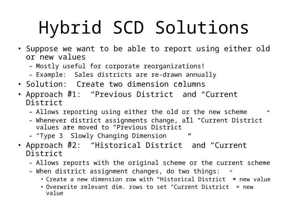
Hybrid SCD Solutions• Suppose we want to be able to report using either old or

new values– Mostly useful for corporate reorganizations!– Example: Sales districts are re-drawn annually

• Solution: Create two dimension columns• Approach #1: “Previous District” and “Current District”

– Allows reporting using either the old or the new scheme– Whenever district assignments change, all “Current District”

values are moved to “Previous District”– “Type 3” Slowly Changing Dimension

• Approach #2: “Historical District” and “Current District”– Allows reports with the original scheme or the current scheme– When district assignment changes, do two things:

• Create a new dimension row with “Historical District” = new value• Overwrite relevant dim. rows to set “Current District” = new value

Dimension Roles• Let’s consider an online auction data mart• We’ll model auction results

– Grain: one fact row per auction.– Bidding history stored in a different fact

• Dimensions:– Auction Start Date– Auction Close Date– Selling User– Buying User– Product

• “Date” and “User” occur twice– Date and User dimensions play multiple roles– Don’t create separate “Auction Start Date” and “Auction End Date”

dimension tables– Do create a single Date dimension table– Do create two separate foreign keys to Date in the fact table

Junk Dimension• Sometimes certain attributes don’t fit nicely into any

dimension– Payment method (Cash vs. Credit Card vs. Check)– Bagging type (Paper vs. Plastic vs. None)

• Create one or more “miscellaneous” dimensions– Group together several leftover attributes as a dimension even if

they aren’t logically related– Reduces number of dimension tables, width of fact table– Works best if leftover attributes are

• Few in number• Low in cardinality• Correlated

– Example: 10 binary flags → no more than 210=1024 dim. rows• Some alternatives

– Each leftover attribute becomes its own dimension– Eliminate leftover attributes that are not useful

International Issues

• International organizations often have facts denominated in different currencies– Some transactions are in dollars, others in Euros, still

others in yen, etc.• Reporting requirements may be diverse

– Standard currency vs. local currency– Historical exchange rate vs. current exchange rate

• Time zones cause a similar problem– Sometimes local time is most meaningful

• E.g. buying patterns are different in morning vs. afternoon– Sometimes standardized time (e.g. GMT) is better

• Correctly express relative order of events

Handling Multiple Currencies

• Add a Currency dimension to the fact table– Values are US Dollars, Yen, Euros, etc.

• Each currency-denominated fact gets 2 fact columns– One column uses the local currency of the transaction– The other column stores the equivalent value in standard

currency– Currency dimension is used to indicate the units being used in

the local currency column– Historical exchange rate in effect the day of the transaction is

used for the conversion

• Create a special currency conversion table– Store current conversion factor between each pair of currencies– Used to generate reports in any currency of interest

Multi-Currency Example

Product Date Currency AmtLocal AmtUSD

443 87 1 400 400

1287 87 4 1250 1447

34 88 2 3500 380

Key Name Abrv Country

1 US Dollar USD USA

2 Japanese Yen JPY Japan

3 Pound Sterling GBP UK

4 Euro EUR Europe

Currency Dimension

Sales Fact

From To Factor

1 2 111.3

1 3 .562

1 4 .814

2 1 .0089

… … …

Conversion Table

Master-Detail Facts

• Consider order data from an e-commerce site• Each Order consists of a series of Lineitems• Each Lineitem represents one product that is

purchased• Measurements are calculated at different levels

– Each Lineitem has Quantity and Price– Each Order has Tax, Discount, and ShippingFee

• Natural design: two fact tables, different grains– Orders fact table with 1 row per order– Lineitem fact table with 1 row per line item

Orders and Lineitems

• Dimensions– Date– Customer– OrderID (degenerate)

• Fact Columns– Tax– Discount– ShippingFee– TotalPrice

• Dimensions– Date– Customer– Product– OrderID (degenerate)

• Fact Columns– Quantity– Price

Orders Fact Lineitem Fact

A Problem with the Design

• Difficult to report on revenue by product• Orders fact lacks Product dimension

– Adding Product would violate the grain• Lineitem fact lacks important revenue data

– Effects of discount, tax, shipping are important– But they are not captured at the lineitem level!

• Solution: allocation of master-level facts to detail-level– Add Tax, Discount, and ShippingFee columns to the Lineitem

fact table– Distribute Tax, Discount, and ShippingFee for the order among

its component line items– Sum of allocated Tax for all line items in an order = actual overall

Tax for that order– Different allocation policies are possible

Fact Allocation Policies• Consider an order consisting of

– A pillow– A bowling ball– A diamond ring

• How should the shipping cost be allocated?– By weight– By volume– By value

• Different policies yield to quite different results– Organizational politics can come into play– If the org. has a standard allocation policy, use it.– Otherwise, try to agree on one– Otherwise, provide all alternatives!

• Activity-based costing is a related concept– Methodology for allocating costs of administrative overheads

• Data warehousing projects can have useful side-effects

Accumulating Snapshot Facts

• Accumulating Snapshot is a third type of fact table– Transactional and Snapshot were already discussed– Not as common as the other two

• Useful for pipelined processes– Process proceeds through a series of stages– 1 fact row tracks an entire process through its lifetime– Best for short-lived processes with linear workflow– Example: Order fulfillment for custom manufacturing

• Order placed → Release to Mfg → Finished Goods Inventory → Shipped → Delivered → Invoiced → Returned

• Characteristics of accumulating snapshot facts– Fact row is updated multiple times during process lifetime

• Different from append-only Transactional and Snapshot facts– Separate date dimension roles for each milestone– Numeric fact columns corresponding to various stages

Querying Accumulating Snapshots

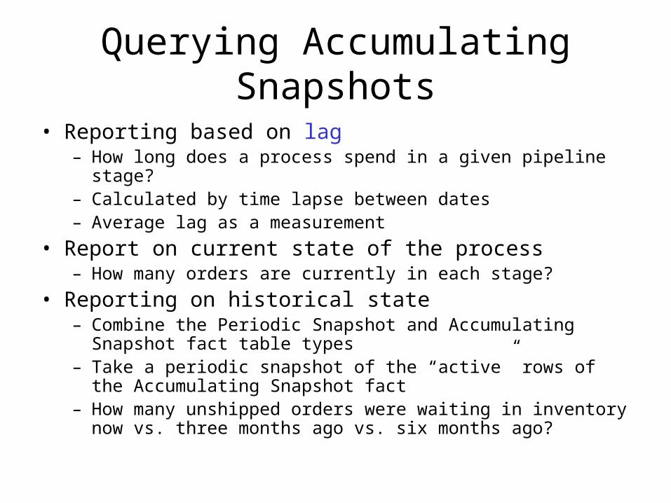
• Reporting based on lag– How long does a process spend in a given pipeline stage?– Calculated by time lapse between dates– Average lag as a measurement

• Report on current state of the process– How many orders are currently in each stage?

• Reporting on historical state– Combine the Periodic Snapshot and Accumulating Snapshot fact

table types– Take a periodic snapshot of the “active” rows of the

Accumulating Snapshot fact– How many unshipped orders were waiting in inventory now vs.

three months ago vs. six months ago?